11email: ahmed_bhayat@hotmail.com 22institutetext: Czech Technical University in Prague, Czech Republic
22email: martin.suda@cvut.cz
A Higher-Order Vampire (Short Paper)
![[Uncaptioned image]](/html/2407.05208/assets/x1.png) Martin Suda
Martin Suda![[Uncaptioned image]](/html/2407.05208/assets/x2.png)
Abstract
The support for higher-order reasoning in the Vampire theorem prover has recently been completely reworked. This rework consists of new theoretical ideas, a new implementation, and a dedicated strategy schedule. The theoretical ideas are still under development, so we discuss them at a high level in this paper. We also describe the implementation of the calculus in the Vampire theorem prover, the strategy schedule construction and several empirical performance statistics.
Keywords:
Vampire Higher-Order Strategy Scheduling.1 Introduction
The Vampire prover [15] has supported higher-order reasoning since 2019 [7]. Until recently, this support was via a translation from higher-order logic (HOL) to polymorphic first-order logic using combinators. The approach had positives, specifically it avoided the need for higher-order unification. However, our experience suggested that for problems requiring complex unifiers, the approach was not competitive with calculi that do rely on higher-order unification. This intuition was supported by results at the CASC system competition [25].
Due to this, we recently devised an entirely new higher-order superposition calculus. This time we based our calculus on a standard presentation of HOL. The key idea behind our calculus is that rather than using full higher-order unification, we use a depth-bounded version. That is, when searching for higher-order unifiers, when some predefined number of projection and imitation steps have taken place, the search is backtracked. The crucial difference in our approach to similar approaches is that rather than failing on reaching the depth limit, we turn the set of remaining unification pairs into negative constraint literals which are returned along with the substitution formed until that point. This is similar to recent developments in the field of theory reasoning [6].
The new calculus has now been implemented in Vampire along with a dedicated strategy schedule. Together these developments propelled Vampire to first place in the THF division of the 2023 edition of the CASC competition.111https://tptp.org/CASC/29/WWWFiles/DivisionSummary1.html As the completeness of the calculus is an open question which we are working on, we have to date not published a description of the calculus.
In this paper, we describe the calculus, discuss its implementation in Vampire and also provide some details of the strategy schedule and its formation.
2 Preliminaries
We assume familiarity with higher-order logic and higher-order unification. Detailed presentations of these can be found in recent literature [5, 3, 29]
We work with a rank-1 polymorphic, clausal, higher-order logic. For the syntax of the logic we follow a more-or-less standard presentation such as that of Bentkamp et al. [3]. Higher-order applications such as contain subterms with no first-order equivalents such as and . We refer to these as prefix subterms. We represent term variables with , function symbols with , and terms with and . To keep the presentation simple, we omit typing information from our terms.
A substitution is a mapping of variables to terms. Unification is the process of finding a substitution for terms and such that for some definition of equality () of interest. It is well known that first-order syntactic unification is decidable and unique most general unifiers exists. For the higher-order case, unification is not decidable, and the set of incomparable unifiers is potentially infinite. A commonly used higher-order unification procedure for enumerating unifiers is Huet’s preunification routine [13]. Unlike full higher-order unification, preunification does not attempt to unify terms if both have variable head symbols. Thus, preunification does not require infinitely branching rules unlike full higher-order unification [29].
The two main rules that extend first-order unification in Huet’s procedure are projection adn imitation. We provide a flavour of these via an example. Consider unifying terms and . In searching for a suitable instantiation of the variable , we can either attempt to copy the head symbol of leading to the substitution , or we can bring one of ’s arguments to the head position leading to the substitution . The first is known as imitation and the second as projetcion.
We use the concept of a depthn unifier. We do not define the term formally, but provide an intuitive understanding. Consider a higher-order preunification algorithm. Any substitution formed by following a path of the unification tree, starting from the root, that contains exactly imitation and projection steps, or reaches a leaf using fewer than such steps, is a depthn unifier. For terms and , let be the set of all depthn unifiers of and . Note that this set is finite as we are assuming preunification and hence the tree is finitely branching.
For terms and , for each depthn unifier , we associate a set of negative equality literals formed by turning the unification pairs that remain when the depth limit is reached into negative equalities. In the case is an actual unifier of and , is of course the empty set.
To make this clearer, consider the unification tree presented in Figure 1. There are two depth2 unifiers labelled and in the figure. Related to these, we have . There are four depth3 unifiers (not shown in the figure) and zero depthn unifiers for for .

3 Calculus
Our calculus is parameterised by a selection function and an ordering . Together these give rise to the concept of literals being (strictly) -eligible with respect to a substitution [3]. When discussing eligibility we drop and and rely on the context to make these clear. We call a literal , where both and have variable heads, a flex-flex literal. Such a literal is never selected in the calculus. We present the primary inference rule, Sup, below.
Sup
In the rule above, we use to denote either a positive or negative equality. We use to denote that is a first-order subterm of . That is, a non-prefix subterm that is not below a lambda. The side conditions of the inference are , is not a variable, is strictly eligible in the left premise, is eligible in the right premise, and the other standard ordering conditions. The remaining core inference rules are EqRes and EqFact.
EqFact
EqRes
For both rules, . For EqFact, is eligble in the premise and for EqRes is eligble. We also include inferences ArgCong (see [4]), and FlexFlexSimp which derives the empty clause, , from a clause containing only flex-flex literals.
ArgCong
FlexFlexSimp
For ArgCong, is eligible in the premise, is the type unifier of and and is a fresh variable. In our implementation, the depth parameter is set via a user option. In the case it is set to 0, the following pair of inferences are added to the calculus.
Imitate
Project
Where ranges from 1 to in Imitate and 1 to in Project, and each is a fresh variable. The literals are eligible in the premises and is the arity of , the projected variable. The idea behind introducing these rules is to facilitate the instantiation of head variables with suitable lambda terms when this is not being done as part of unification. Our intuition is that by intertwining the unification and calculus rules in the spirit of the EP calculus [21], the need for explosive rules (such as FluidSup[3]) that simulate superposition underneath variables is removed. The examples we present below support this intuition. Besides the core inference rules, the calculus has a set of rules to handle reasoning about Boolean terms. These are similar to rules discussed in the literature [30, 20]. Extensionality is supported either via an axiom or by using unification with abstraction as described by Bhayat [5]. Similarly, Hilbert choice can be supported via a lightweight inference in the manner of Leo-III [20] or via the addition of the Skolemized choice axiom. The calculus also contains various well-known simplification rules such as Demodulation and Subsumption.
Soundness and Completeness. The soundness of the calculus described above is relatively straightforward to show. On the other hand, the completeness of the calculus with respect to Henkin semantics is an open question. We hypothesise that given the right ordering, and with tuning of inference side conditions, the depth0 variant of the calculus (with the Imitate and Project rules) is refutationally complete. A proof is unlikely to be straightforward due to the fact that we do not select flex-flex literals.
Example 1
Consider the following unsatisfiable clause set. Assume a depth of 1. Selected literals are underlined.
An EqRes binds to and results in . An EqRes on binds to and results in . A final EqRes on binds to and results in from which it is trivial to obtain the empty clause .
Example 2 (Example 1 of Bentkamp et al. [4])
Consider the following unsatisfiable clause set. Assume the depth0 version of the calculus.
An EqRes inference on results in . An Imitate inference on the first literal of followed by the application of the substitution and some -reduction results in . A further double application of EqRes gives us . We again carry out Imitate on the first literal followed by an EqRes to leave us with . We can now carry out a Sup inference between and resulting in from which it is simple to derive via an application of Imitate on either the first or the third literal. Note, that the empty clause was derived without the need for an inference that simulates superposition underneath variables, unlike in [4].
4 Implementation
The calculus described above, along with a dedicated strategy schedule, has been implemented in the Vampire theorem prover.222See http://bit.ly/3vBQLi4 for the release, https://bit.ly/3Hl3lES for the code. Vampire natively supports rank-1 polymorphic first-order logic. Therefore, we translate higher-order terms into polymorphic first-order terms using the well known applicative encoding. Note, that we use the symbol , in a first-order type, to separate the argument types from the return type. It should not be confused with the binary, higher-order function type constructor that we assume to be in the type signature. Application is represented by a polymorphic symbol . Lambda terms are stored internally using De Bruijn indices. A lambda is represented by a polymorphic symbol . De Bruijn indices are represented by a family of polymorphic symbols for . Thus, the term is represented internally as . The term is represented internally (now ignoring type arguments) as .
Some of the most important options available are: hol_unif_depth to control the depth unification proceeds to, funx_ext to control how function extensionality is handled, cnf_on_the_fly to control how eager or lazy the clausification algorithm is, and applicative_unif which replaces higher-order unification with (applicative) first-order unification. This is surprisingly helpful in some cases. Besides for the options listed above, there are many other higher-order specific options as well as options that impact both higher-order and first-order reasoning. These options can be viewed by building Vampire and running with --help.
5 Strategies and the Schedule
We generally followed the Spider [27] methodology for strategy discovery and schedule creation. This starts with randomly sampling strategies to solve as-of-yet unsolved problems (or improve the best known time for problems already known to be solvable). Each newly discovered strategy is optimized with local search to work even better on the single problem which it just solved. This is done by trying out alternative values for each option, possibly in several rounds. A variant of the strategy that improves the solution time or at least uses a default value of an option is preferred. The final strategy is then evaluated on the totality of all considered problems and the process repeats.
In our case, we sought strategies to cover the TH0 problems of the TPTP library [24] version 8.1.2. The strategy space consisted of 87 options inherited from first-order Vampire and 26 dedicated higher-order options. To sample a random strategy, we considered each option separately and picked its value based on a guess of how useful each is. (E.g., for applicative_unif we used the relative frequencies of on: 3, off: 10.) During the strategy discovery process we adapted the maximum running time per problem, both for the random probes several times and for the final strategy evaluation: from the order of up to . In total, we collected strategies over the course of approximately two weeks of continuous 60 core CPU computation. The strategies cover unsatisfiable problems, including 50 problems of TPTP rating 1.0 (which means these problems were not officially solved by an ATP before).
Once a sufficiently rich set of strategies gets discovered and evaluated, schedule building can be posed as a constraint programming task in which one seeks to allot time slices to individual strategies to cover as many problems as possible while not exceeding a given overall time bound [12, 19]. We had a good experience with a weighted set cover formulation and applying a greedy algorithm [9]: starting from an empty schedule, at any point we decide to extend it by scheduling a strategy for additional units of time if this step is currently the best among all possible strategy extensions in terms of “the number of problems that will additionally get covered divided by ”. This greedy approach does not guarantee an optimal result, but runs in polynomial time and gives a meaningful answer uniformly for any overall time bound . (See [8] for more details).
Our final higher-order schedule tries to cover, in this greedy sense, as many problems as possible at several increasing time bounds: starting from , , and bounds relevant for the impatient users, all the way up to the CASC limit of 16 minutes (2 minutes on 8 cores) and further beyond. In the end, it makes use of out of the available strategies and manages to cover all the known-to-be-solvable problems in a bit less than 1 hour of single core computation. We stress that our final schedule is a single monolithic sequence and does not branch based on any problems’ characteristics or features.333One additional interesting aspect of our schedule building approach (left out due to space restrictions, but see Appendix 0.A for more details) is that we employ input shuffling and prover randomization [23] and thus treat our strategies as Las Vegas algorithms, whose running time or even success/failure may depend on chance.
Most important options:
| an option | default | # problems not solvable without non-default |
|---|---|---|
| cnf_on_the_fly | eager | 102 |
| applicative_unif | off | 56 |
| equality_to_equiv | off | 24 |
| hol_unif_depth | 2 | 20 |
| func_ext | abstraction | 12 |
In Table 1, we list the first five options sorted in descending order of “how many problems we would not be able to cover if the given option could not be varied in strategies.” (In other words, as if the listed default value was “wired-in” to the prover code.)
Based on existing research [28], it is unsurprising to see that varying clausification has a large impact. Likewise, for varying the unification depth. What is perhaps more surprising is that replacing higher-order unification with applicative first-order unification can be beneficial. equality_to_equiv turns equality between Boolean terms into equivalence before the original clausification pass is carried out. The effectiveness of this option is also somewhat surprising.
Performance statistics:
| single strategy | 1811 | 1949 | 2041 | 2094 | ||
|---|---|---|---|---|---|---|
| our schedule | 2067 | 2436 | 2584 | 2642 | 2691 | 2775 |
It is long known [26, 31] that a strategy schedule can improve over the performance of a single good strategy by large margin. Table 2 confirms this phenomenon for our case. For this comparison we selected one of the best performing (at the time limit mark) single strategies that we had previously evaluated. From the higher-order perspective, the strategy is interesting for setting hol_unif_depth to 4 and supporting choice reasoning via an inference rule (choice_reasoning on).444Otherwise, it uses Vampire’s default setting, except for relying on an incomplete literal selection function [11] and using a relative high naming threshold [17], i.e., being reluctant to introduce new names for subformulas during clausification.
Although our schedule has been developed on (and for) the TH0 TPTP problems, it helps the new higher-order Vampire solve more problems of other origin too. Of the Sledgehammer problems exported by Desharnais et al. in their last prover comparison [10], namely the 5000 problems denoted in their work TH0-, Vampire can now solve compared to obtained by Desharnais et al. with the previous Vampire version (both under per problem).555 Our experiments were run on Intel®Xeon®Gold 6140 CPU @ , Desharnais et al. [10] used StarExec [22] with Intel®Xeon®CPU E5-2609 @ nodes.
We remark that we also developed a different schedule specifically adapted to Sledgehammer problems (in various TPTP dialects, i.e., not just TH0), which is now available to the Isabelle [16] users since the September 2023 release.
6 Related Work
The idea to intertwine superposition and unification appears in earlier work, particularly in the EP calculus implemented in Leo-III [21]. The main differences between our calculus and EP are:
-
1.
We do not move first-order unification to the calculus level. Hence, there are no equivalents to the Triv, Bind and Decomp rules of EP.
-
2.
Our Project and Imitate rules are instances of EP’s FlexRigid rule. We do not include an equivalent to EP’s FlexFlex rule since we never select flex-flex literals. Instead, we leave such literals until one of the head variables becomes instantiated, or the clause only contains flex-flex literals at which point FlexFlexSimp can be applied.
-
3.
Our core inference rules are parameterised by a selection function and an ordering.
-
4.
Whilst EP always applies unification lazily, our calculus can control how lazily unification is carried out by varying the depth bound.666Our understanding based on [20] is that the implementation of EP in Leo-III does make use of orderings as well as eager unification. It is not clear to us from the exposition how these are applied.
We also incorporate more recent work on higher-order superposition, mainly from the Matryoshka project [28, 3]. Of course, the use of constraints in automated reasoning extends far beyond the realm of higher-order logic. They have been researched in the context of theory reasoning [18, 14] and basic superposition [2].
7 Conclusion
In this paper, we have presented a new higher-order superposition calculus and discussed its implementation in Vampire. We have also described the new higher-order schedule created. The combination of calculus, implementation and schedule have already proven effective. However, we believe that there is great room for further exploration and improvement. On the theoretical side, we wish to prove refutational completeness of the calculus (or a variant thereof). On the practical side, we wish to refine the implementation, most notably by adding additional simplification rules.
7.0.1 Acknowledgements
The second author was supported by project CORESENSE no. 101070254 under the Horizon Europe programme and project RICAIP no. 857306 under the EU-H2020 programme.
References
- [1] CASC design and organization. https://www.tptp.org/CASC/29/Design.html, Accessed: January 2024
- [2] Bachmair, L., Ganzinger, H., Lynch, C., Snyder, W.: Basic paramodulation and superposition. In: CADE. LNAI, vol. 607. Springer (1992)
- [3] Bentkamp, A., Blanchette, J., Tourret, S., Vukmirović, P.: Superposition for higher-order logic. Journal of Automated Reasoning 67(1) (2023)
- [4] Bentkamp, A., Blanchette, J.C., Tourret, S., Vukmirović, P., Waldmann, U.: Superposition with lambdas. In: CADE. LNAI, vol. 11716, pp. 55–73. Springer (2019)
- [5] Bhayat, A.: Automated Theorem Proving in Higher-Order Logic. Ph.D. thesis (2015)
- [6] Bhayat, A., Korovin, K., Kovács, L., Schoisswohl, J.: Refining unification with abstraction. In: LPAR. pp. 36–47 (2023)
- [7] Bhayat, A., Reger, G.: A combinator-based superposition calculus for higher-order logic. In: IJCAR. LNAI, vol. 12166, pp. 278–296. Springer (2020)
- [8] Bártek, F., Chvalovský, K., Suda, M.: Regularization in spider-style strategy discovery and schedule construction. In: IJCAR (2024), accepted
- [9] Chvátal, V.: A greedy heuristic for the set-covering problem. Math. Oper. Res. 4(3), 233–235 (1979)
- [10] Desharnais, M., Vukmirović, P., Blanchette, J., Wenzel, M.: Seventeen provers under the hammer. In: ITP. LIPIcs, vol. 237, pp. 8:1–8:18. Schloss Dagstuhl - Leibniz-Zentrum für Informatik (2022)
- [11] Hoder, K., Reger, G., Suda, M., Voronkov, A.: Selecting the selection. In: Olivetti, N., Tiwari, A. (eds.) IJCAR. LNCS, vol. 9706, pp. 313–329. Springer (2016)
- [12] Holden, E.K., Korovin, K.: Heterogeneous heuristic optimisation and scheduling for first-order theorem proving. In: CICM. LNCS, vol. 12833, pp. 107–123. Springer (2021)
- [13] Huet, G.P.: A unification algorithm for typed -calculus. Theoretical Computer Science 1(1), 27–57 (1975)
- [14] Korovin, K., Kovács, L., Reger, G., Schoisswohl, J., Voronkov, A.: ALASCA: Reasoning in quantified linear arithmetic. In: TACAS. LNCS, vol. 13993, pp. 647–665. Springer (2023)
- [15] Kovács, L., Voronkov, A.: First-order theorem proving and Vampire. In: CAV. LNCS, vol. 8044, pp. 1–35. Springer (2013)
- [16] Nipkow, T., Paulson, L.C., Wenzel, M.: Isabelle/HOL: a proof assistant for higher-order logic, vol. 2283. Springer Science & Business Media (2002)
- [17] Reger, G., Suda, M., Voronkov, A.: New techniques in clausal form generation. In: GCAI. EPiC Series in Computing, vol. 41, pp. 11–23. EasyChair (2016)
- [18] Reger, G., Suda, M., Voronkov, A.: Unification with abstraction and theory instantiation in saturation-based reasoning. In: TACAS. LNCS, vol. 10805, pp. 3–22. Springer (2018)
- [19] Schurr, H.: Optimal strategy schedules for everyone. In: PAAR. CEUR Workshop Proceedings, vol. 3201. CEUR-WS.org (2022)
- [20] Steen, A.: Extensional paramodulation for higher-order logic and its effective implementation Leo-III. Ph.D. thesis (2018)
- [21] Steen, A., Benzmüller, C.: Extensional higher-order paramodulation in Leo-III. Journal of Automated Reasoning 65(6), 775–807 (2021)
- [22] Stump, A., Sutcliffe, G., Tinelli, C.: Starexec: A cross-community infrastructure for logic solving. In: IJCAR. LNCS, vol. 8562, pp. 367–373. Springer (2014)
- [23] Suda, M.: Vampire getting noisy: Will random bits help conquer chaos? (system description). In: IJCAR. LNCS, vol. 13385, pp. 659–667. Springer (2022)
- [24] Sutcliffe, G.: The TPTP Problem Library and Associated Infrastructure. From CNF to TH0, TPTP v6.4.0. Journal of Automated Reasoning 59(4), 483–502 (2017)
- [25] Sutcliffe, G., Suttner, C.: The state of CASC. AI Communications pp. 35–48 (2006)
- [26] Tammet, T.: Towards efficient subsumption. In: Kirchner, C., Kirchner, H. (eds.) CADE. LNCS, vol. 1421, pp. 427–441. Springer (1998)
- [27] Voronkov, A.: Spider: Learning in the sea of options. In: Vampire23: The 7th Vampire Workshop (2023), https://easychair.org/smart-program/Vampire23/2023-07-05.html#talk:223833, to appear.
- [28] Vukmirović, P., Bentkamp, A., Blanchette, J., Cruanes, S., Nummelin, V., Tourret, S.: Making higher-order superposition work. In: CADE. LNAI, vol. 12699, pp. 415–432. Springer (2021)
- [29] Vukmirović, P., Bentkamp, A., Nummelin, V.: Efficient full higher-order unification. Logical Methods in Computer Science 17 (2021)
- [30] Vukmirović, P., Nummelin, V.: Boolean reasoning in a higher-order superposition prover. In: PAAR. pp. 148–166 (2020)
- [31] Wolf, A., Letz, R.: Strategy parallelism in automated theorem proving. In: Cook, D.J. (ed.) FLAIRS. pp. 142–146. AAAI Press (1998)
Appendix 0.A Note on Probabilistic Schedule Building
CASC organizers randomly shuffle the input problems to make sure that “no system receives an advantage or disadvantage due to the specific presentation” [1]. At the same time, it is well known that with a saturation-based prover even such small changes may have dramatic effect on strategy’s running time [23]. To create a schedule resilient to input shuffling, we actually sampled our strategies with Vampire’s internal shuffling enabled, ready to evaluate a strategy on a problem more than once (under different random seeds) to establish an estimate of its runtime distribution.
We then adapted the greedy algorithm to seek to cover problems “in expectation”. By this we mean that a strategy can score a fractional point for solving a problem (if it solves it, e.g., in of its runs), where appropriately smaller fractions are awarded for problems already partially covered.
Our final schedule is then also executed under fresh random seeds and its performance, therefore, slightly varies depending on chance.
The estimate of a runtime distribution of a strategy on a given problem is explained on an example in Table 3. Note that we work with two possible failure modes: a deliberate giving up, which may happen with incomplete strategies, and termination through a timeout. The difference in interpretation is that a timeout could later have turned into a success if we had waited longer.
| time points and intervals | run1 | run2 | run3 | run4 | probability |
|---|---|---|---|---|---|
| r | r | r | r | 0/4 | |
| success | r | r | r | ||
| r | r | r | 1/4 | ||
| gave up | r | r | |||
| r | r | 1/4 | |||
| timeout | r | ||||
| r | 1/3 | ||||
| success | |||||
| 2/3 |
We initially evaluate each strategy only once, as described in the main text. We then run the greedy schedule construction algorithm multiple times and iteratively reevaluate strategies on problems which the greedy algorithm reports are getting covered by them, thus getting gradually better probability estimates at points where they matter.
Covering problems in expectation uses the assumption of strategy independence. For example, knowing that the current schedule solves problem with a probability of 0.6 and a new strategy added for units of time solves with the probability , adding to the schedule will improve the coverage of from 0.6 to , that is, by . When computing the weight for the greedy covering, the strategy will accrue these points for contributing to solving problem .
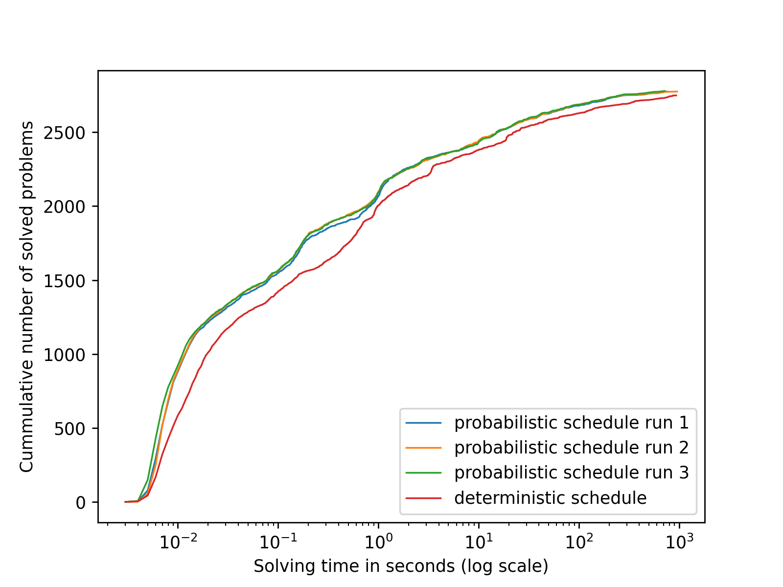
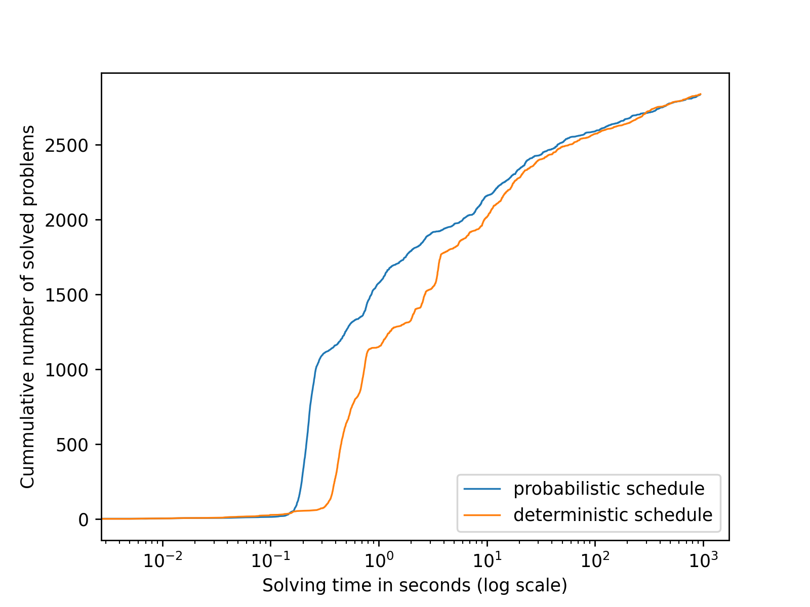
The performance impact of the probabilistic approach can be observed in Figure 2. We can see that there is a substantial difference in the lower time limit bracket (around 90 problems at on TPTP and 426 problems on the Sledgehammer problems), which becomes less pronounced with higher time limits (50 problems at on TPTP and 31 on Sledgehammer there). The gap completely closes at around per problem on the Sledgehammer problems, from which point the deterministic schedule even mildly dominates. We currently do not have a good explanation for this last observation.
We conclude that investing into developing a probabilistic schedule on higher-order problems does pay off, especially at low time limits desired in applications with an impatient user, and carries over to in-training-unseen problems.
