Measuring gravitational wave memory with LISA
Abstract
Gravitational wave (GW) astronomy has revolutionized our capacity to explore nature. The next generation of observatories, among which the space-borne detector Laser Interferometer Space Antenna LISA, is expected to yield orders of magnitude of signal-to-noise ratio improvement, and reach fainter and novel features of General Relativity. Among them, an exciting possibility is the detection of GW memory. Interpreted as a permanent deformation of the background spacetime after a GW perturbation has passed through the detector, GW memory offers a novel avenue to proof-test General Relativity, access the non-linear nature of gravity, and provide complementary information for a better characterization of the GW source. Previous studies have shown that GW memory detection from individual mergers of massive black hole binaries is expected with LISA. However, these works have not simulated the proper time domain response of the detector to the GW memory. This work is filling this gap and presents the detection prospects of LISA regarding GW memory and the expected signature of GW memory on the data-streams using the most up-to-date LISA consortium simulations of the response, as well as GW memory time-series computation inherited from numerical relativity. We will confront the LISA observation window to massive black hole binary mergers’ population forecasted with the state-of-the-art population models and evaluate the odds and the expected accuracies regarding GW memory observations in the LISA lifetime. We conclude that GW memory will be a key feature of several events detected by LISA, and will help to exploit the scientific potential of the mission fully.
I Introduction
When a flux of matter (e.g. unbound objects) or radiation goes through a region of space-time, the final metric of that region returns to its original (Minkowksi) form, but the relative distances of freely falling observers are permanently modified with respect to their original ones. This is called gravitational wave memory effect, see e.g. [1, 2, 3, 4], or, in recent language, displacement memory, and is the dominant of several effects related to the changes of asymptotic states from the passage of radiation [5, 6, 7, 8, 9, 10]. Remarkably, these effects are intimately connected to the asymptotic structure of space-time in General Relativity, namely with the symmetries of the BMS group [11, 12] and soft theorems [13, 14].
In this work, we will focus on the Gravitational Wave (GW) memory generated by the passage of gravitational flux, which is usually called non-linear or null memory to differentiate it from the linear or ordinary memory, which is related to the flux of other sorts of radiation or matter. Moreover, we will restrict to the displacement memory and not consider other subdominant effects, such as the spin [9] or the center-of-mass [10, 15] memories.
The origin of GW memory stems from the non-linear nature of General Relativity: gravitational radiation generates gravitational waves at second order, that eventually generate the memory [4, 16, 17, 18, 19, 20, 21]. This explains some of the features of the effect since its magnitude relative to that of the linear GWs and its typical time scale or its angular dependence are related to the flux emitted by the linear signal. As a result, the properties of the GW memory strongly differ from those of the primordial radiation and, despite being a small effect, GW memory may carry key complementary information from the primary signal111Furthermore, being a term that may accumulate with time, its final size may also be larger than otherwise expected [22].. For instance, it may allow one to break the degeneracy between luminosity distance and inclination [23, 24] or between the merger of binary black holes or neutron stars [25, 26]. The use of GW memory has also been proposed to test the asymptotic symmetries of space-time [27], or as a part of consistency tests of waveform models exploiting balance laws [28, 29]. Furthermore, since GW memory probes the non-linear nature of gravitation, it is natural to expect changes in modified theories of gravity [30, 31, 32, 33]. Finally, the different frequency span of the GW memory as compared to the primary signal allows looking for merger events of primordial frequencies higher than the detector band [34] and even search for the same events in ground-base and space-borne detectors [35]. In conclusion, the detection of GW memory will open several possibilities to probe astrophysics and fundamental physics with GWs.
GW observations have so far not detected GW memory. This is mainly due to the smallness of the effect and is true both for binary black hole coalescences observed in LIGO/Virgo data [36, 37, 38, 39] and supermassive black hole coalescences that may explain Pulsar Timing Arrays data [40, 41, 42]. In fact, it is not expected for current ground-based interferometers to detect the memory from the coalescence of single binary compact objects. Instead, it has been suggested that the combination of events with GW memory Signal-to-Noise Ratio (SNR) below threshold over 2 to 5 years may be enough to reach detection in these set-ups [7]. The prospects of detecting the memory from single events are more promising for the next generation of detectors, either ground-based, such as the ET [43] and CE [44], the space-based interferometers the Laser Interferometer Space Antenna (LISA) and TianQin [7, 23, 45, 46, 47, 48, 49, 50] or SKA [51, 52].
In this paper, we focus on the characteristic imprint of the memory on the LISA detector from the coalescence of Massive Black Holes (MBHs) that merge in the frequency band between Hz and . These events will have an extraordinarily high SNR, especially during the merger, when most of the memory is created. Consequently, these objects are the most promising source of detectable GW memory. Recent works [23, 49, 50] have confirmed that several MBH mergers will have an SNR of the GW memory sufficiently high to claim detection, though the expected number varies considerably depending on the astrophysical population considered. Building on these results, one of our main goals is to improve them by investigating the GW memory with the full time-domain response of LISA, based on Time Delay Interferometry (TDI) and its most updated noise characterization. Addressing the robustness of the detection of GW memory when TDI is considered is essential to build a solid understanding of the imprint of this effect, especially if one aims at using it as an additional source of information complementary to the leading oscillatory signal. We devote the rest of the paper to the first investigation in this direction for the LISA mission.
Compared to previous work, we also consider new waveforms that directly contain the GW memory [53] which, for non-precessing binaries, is mainly contained in the (2,0) mode [45]. We also investigate the overlap of the memory and additional oscillatory features excited during the merger and the ringdown, both present in the (2,0), and we discuss potential strategies to distinguish the two. We further perform a broad study of the parameter space of the binary merger by varying the mass ratio of the two black holes and the amplitude of the aligned spin of the sources, though we will not consider the presence of precession or non-trivial eccentricities. The detectability of GW memory by LISA will be assessed with state-of-the-art population models of MBHs described in Refs. [54, 55] (and based on previous work presented in [56, 57, 58]).
The paper is organized as follows. In Sec. II we describe the necessary tools for the subsequent analysis, such as the TDI processing, the LISA noise characterization and the waveform models. In Sec. III, we comprehensively describe how the displacement memory impacts the signal of LISA. In Sec. IV we discuss the signal-to-noise ratio and the detectability predictions. Sec. V is devoted to the study of MBHs mergers and the prospect of detecting memory from them in LISA. In Sec. VI, we explore the particular dependence of the memory SNR w.r.t. mass ratio and spin. Finally, we discuss our conclusions and outlook in Sec. VII.
II Displacement Memory imprints on LISA interferometric data
GW interferometers, either ground or space-based, are not designed to observe a permanent shift of the strain because they are sensitive to a limited frequency band. As a result, they cannot detect the permanent offset from the GW memory. However, the time-dependent transition in strain induced by the GW memory at the detector location does exhibit significant spectral content at low frequencies, which may be detected. LISA’s sensitivity band span GWs between Hz and [59]. Its better sensitivity at low frequencies as compared to current ground-based interferometers implies that it is a better detector of GW memory for the (MBH) mergers that have support at its frequency sensitivity peak (mHz). The proper determination of LISA’s sensitivity to GW memory requires a full time-domain simulation of the projection of the signal onto the laser antenna response (down to TDI data streams).
In this section, we show a comprehensive End-To-End (E2E) simulation of the LISA time-domain response to the GW memory using the most up-to-date LISA consortium simulations (LISAGWResponse [60, 61], LISAInstrument [62, 63]) and post-processing software (PyTDI [64]).
Furthermore, we consider the most accurate model to date for the memory, based on numerical simulations contained in the
NRHybSur3dq8_CCE surrogate model [53]. This model is trained on numerical waveforms limited to mass-ratio and spins aligned to the angular momentum of the binary with amplitude (the model does not include precession or eccentricity). This is the first waveform model that includes the full memory mode and is calibrated to Numerical Relativity simulations, something possible thanks to the use of the Cauchy-Characteristic Evolution (CCE) extraction procedure of the strain from numerical relativity simulations [65] and it is now implemented in the SXS catalogue [66, 12].
As previous waveform models did not include the subdominant mode, one had to correct them by adding the memory at a later moment. This could be done by computing the memory from the primary waveform (e.g. with the code
GWMemory222This method does not capture the linear memory component generated from the black hole kick. However, this has been shown to be a much subdominant contribution [67]. [68] or using balance laws [11], as done in [69, 70, 38, 38, 49]. Only recently, a waveform model for the mode which includes both the memory and the ringdown components was implemented as an extension of the computationally efficient IMRPhenomTHM model that can be used in the future for extensive Bayesian parameter estimation [71].
II.1 GW memory model and simulation
To assess the detectability of the memory, it is important to isolate it in the total GW strain. Here, we call the memory signal the part of the GW that is generated merely by the energy flux emitted in primary GWs. For non-precessing signals, the memory mainly appears in the mode [29], which is a geometric consequence of the fact that most of the energy in GWs is released into the mode [45]. On the other hand, in the mode there are also oscillating contributions excited during the merger and the ringdown, and both of them are present in the NRHybSur3dq8_CCE waveforms. To extract the memory from these waveforms, we use the former surrogate model NRHybSur3dq8 [72] (with waveforms defined as ), which does not capture the memory component, but only the oscillating contribution, and define:
| (1) |
This separation is shown in Figure 1, where we show the total waveform (blue) and the mode from the NRHybSur3dq8_CCE model (orange) and from the NRHybSur3dq8 (green) for a merger event with parameters [, , , , ]. On the right panel, it is clear that Eq. (1) allows us to isolate the memory, which resembles a DC signal, from the oscillatory features of the ringdown in the mode. Such differentiation is also evident in the frequency domain, as we explain in Section III.
A better characterization of the GW memory would follow from the BMS strain decomposition discussed in [70], where the contributions from the memory and the oscillating signal in the mode are clearly identified as the energy flux and the changes of the Bondi mass. Since these two quantities are not easily extracted from the NRHybSur3dq8_CCE waveforms, without some post-processing, we will use Eq. (1) to characterize the memory from the numerical waveforms. One can also compute the GW memory from Thorne’s formula [73] (or via balance laws [70]) through the GWMemory package [68], which performs the following integral from the numerical waveforms without GW memory
| (2) |
where is the retarded time and the distance. Since we want to rely on the memory coming directly from numerical simulations, we use Eq. (1) for most of the parameter space. However, we find some differences between the memory computed in this way and the mode computed by Eq. (2) which are more visible at higher mass ratios, as we will discuss in Section VI. These differences may be due to the fact that NRHybSur3dq8_CCE and NRHybSur3dq8 differ in the reference frame in which they are computed333The extrapolated waveforms [72] are in the centre-of-mass frame, while the CCE ones are in the BMS frame [53]. In addition, the surrogates are constructed slightly differently (e.g. the phase misalignment). We thank Lorena Magaña Zertuche for clarifying this point.. We do not know if this is the only reason for the difference, or if the differences between the two methods are also due, e.g., to physical contributions in the ringdown, which are better captured by the numerical simulations. Indeed, we see that the signal in the Fourier domain differs mainly by peaks at frequencies close to the ringdown. Eventually, we verified that both methods yield comparable GW memory SNR for equal mass systems. Throughout this work, we mostly use the one based on numerical simulations (namely Eq. 1), except when systems are considered, where GWMemory code [68] and Equation 2 are preferred. More details about the observed discrepancy between this and GWMemory are given in Appendix B.
II.2 Detector response simulation
The simulation of the detector response requires the projection of the strain time-series computed in Section II.1 onto the space antenna response. For this, one first computes the interferometer’s six single-link time-domain responses to the memory strain time-series using LISAGWResponse [60, 61]. This yields time-series of relative (Doppler) frequency modulation of the laser link frequency caused by the GW crossing over the laser beam path. A comprehensive derivation of the time-domain link response can be found in Appendix A of [74]. The single-link frequency fluctuation data streams are then injected to the PyTDI software [64] in order to synthetize the virtual interferometer (i.e. suppressing primary noises, such as laser [60] and spacecraft jitter noise [75]). This generates the ultimate interferometer time-series, selecting the A, E and T (second generation) variables [76, 77] to work with two independent channels (A and E), sufficient for SNR computations. Keplerian orbits are considered for the constellation spacecraft, both for the single-link response and the time delays in TDI post-processing.
In addition, we performed several processing adjustments to facilitate the computation of the SNR around the merger time. First, the time reception shift of the wave at the detector location is ignored (setting sun_shift = False). This is a parameter specific to LISAGWResponse, where the timing frame for the input strain time series is understood from the location of the Solar System Barycentric (SSB) reference frame barycentre, implying a propagation time until it reaches the space interferometer. This makes the merger time depend on the sky-localization of the source, adding unnecessary complications for our scope here. Second, the time origin was adapted so that the merger time — defined as the time of the maximum amplitude as conventional in literature [78] — is set to be . The time window width around has been set to adapt dynamically to the total mass of the Massive Black Holes Binary (MBHB) system, ensuring to capture most of the oscillatory SNR for events with , and to fully capture the memory SNR for all relevant MBHB masses (). Finally, to avoid biases at low frequencies when representing the waveform in the frequency domain, especially occurring due to edge effects from the restricted time window and the GW memory step-like shape, we apply the Planck-taper window centred on the merger time, as extensively used in GW data analysis [79].
II.3 Noise settings
For the SNR determinations, LISA noise spectra are computed from single-link noise models, merely containing the two dominant secondary noises, i.e. the test mass (TM) acceleration noise and the Optical Metrology System (OMS) noise, and in agreement with the LISA Science Requirement Document (SciRD) [80],
| (3) | |||
| (4) |
We then apply the TDI transfer function matrices on the single-link data streams based on the TDI-2 combinations, defined as
| (5) | ||||
with
| (6) |
There, for example, is the frequency modulation of the laser beam emitted from spacecraft towards spacecraft , and as measured on spacecraft , then accumulating GW modulation along its path. are nested time-delay operators. For example, the second term of Eq. (II.3), , is the time-domain operator used to delay the single-link data by a time shift equal to the light travel time of a laser beam circulating across the spacecraft constellation, starting at spacecraft , making a round trip along arm , then going for a second round trip along arm to finally ending back at spacecraft .
From there, we move to the frequency domain, where we approximate the delay operators as simple phase operators (Eq. (7)),
| (7) |
Arranging the TDI operators as a matrix applied on the single-link noise spectra as in [74], one gets:
| (8) |
with and indexing for the Michelson X, Y, Z channels. Converting to A, E, T TDI channels by a simple change of basis [81]:
| (9) |
one gets the A, E, T noise spectra:
| (10) | |||
| (11) | |||
| (12) |
assuming symmetric performances for , and channels.
In addition to instrumental noise, we add for completeness a -years galactic confusion noise spectrum, equivalent to the residual power left by the unresolved (and non-extracted) GWs from galactic binaries after a -years observation run (minimal expected mission duration) [82, 80].
Finally, it is worth noting that the noise power spectrum required a smoothing treatment at the zero-response frequencies to counteract numerical instabilities when computing the SNR. Processing the single-link noise spectrum, we have considered multiple TDI transfer functions evaluated at distinct epochs of the year and averaged the outputs to get the finally used TDI noise power spectrum. The procedure then provides a year-averaged power spectrum, as well as smoothed-out resonances, which now have a negligible impact on the SNR values.
We finally define the SNR of and memory signals in LISA data as [83]:
| (13) |
where all spectra are one-sided. We combine the 3 TDI channels, summing the individual SNR quadratically:
| (14) |
using the property of , and channels of being approximately independent. Limited frequency range with and is considered in the computation of , making sure that all the memory SNR and most of the mode are captured, for any masses ranging from to .
III Memory signature in LISA data
Equipped with the above state-of-the-art simulation tools for the LISA TDI time-domain response to GW, we can now study the projection of the wave strain, defined as the mode, and of the memory strain, defined as the memory component of the mode explained above.

This is shown for the three different channels A, E and T in Figure (2) for the GW of the same event considered in Figure 1. In the background of the same figure, and attached to the additional right-hand -axis, we trace the mode (down-scaled by ) and the memory strain for a timing reference; the merger time is also indicated with a black dotted line. One observes from Figure 2 that the instrument response function acts as a high-pass filter for the memory signal, significantly reducing the overall amplitude and exhibiting time oscillations. In fact, at low frequency, i.e. for wavelengths longer than the arm length, the instrument response behaves as a high order differentiator [84]. As a result, the TDI output for the memory is mostly determined by , as we show in Appendix A.
This can also be seen in the frequency domain in Figure 3, where we compare the spectra of the injected signals (up) and of the TDI outputs (down). The Fourier Transform (FT) of the memory on the upper panel (orange) scales as at low frequency and it decays at frequencies where is the redshifted mass of the binary. This follows from the fact that, on time scales longer than its rising time, the memory is well approximated by a step-like function around the merger time, whose FT is . At high frequency, the cutoff frequency is given by the duration of the memory saturation , that corresponds to the time window around the merger, during which most of the GW energy is radiated [85]. We also show in Figure 3 the oscillating component of the mode (green). It is interesting to note that the frequency (black dashed) represents a good transition above which this oscillatory component overcomes the memory. Again, this is consistent with identifying the pure memory with the low-frequency signal of the mode.

On the lower panel of Figure 3 we show the spectra of the TDI response to the (2,2) and memory modes of the waveform. Comparing the upper and lower subplots, focusing on the low-frequency memory spectra, we confirm the behavior of the LISA response which, in the long wavelength regime, manifestly approximates as a third-order time differentiator.
We stress that, to recover the expected spectrum of the memory strain shown in the upper panel of Figure 3, some processing of the waveform is needed that is different from the usual one applied to the oscillating wave. In particular, to recover the low-frequency behavior of the memory, we pad the strain to its final value for a sufficiently long time after the end of the generated waveform and use a Planck-taper window function to put the final value gradually to zero. This last step is crucial: otherwise, spectral leaking would completely spoil the weak signal from the memory. The issue of correctly processing the memory has also recently been discussed in [86], where an alternative method to recover a clean spectrum is proposed. However, we found that this issue is not present in the TDI output of the memory shown on the lower panel of Figure 2, since effectively the TDI output is proportional to higher derivatives of the injected signal and the time series naturally goes to zero at the edges.
Further insight into the characterization of the memory in the data is provided by the time-frequency plot of the TDI signals of the primary wave and the memory. As shown in Figure 4, the two signals present a different localization in the time-frequency representation, with the (2,2) mode exhibiting the well-known chirp transient signal, increasing in power towards high frequencies, while the memory is confined to the merger time and relatively spread over frequencies, although with a maximum power frequency distinct from the (2,2) merger frequency.

| Baseline | inclination | lat. | long. | pixel | ||
|---|---|---|---|---|---|---|
| 1. Conservative | 2.5 | 0.0 | 1.047 | 0.62 | 0.20 | 145 |
| 2. Optimistic | 1.0 | 0.0 | 1.571 | 0.52 | 3.24 | 192 |
| 3. Opt. & Spin. | 1.0 | 0.8 | 1.571 | 0.52 | 3.24 | 192 |
IV Signal-to-noise ratio and detectability predictions
We begin by examining the SNR of the primary wave and the memory as a function of sky position, which is important for two main reasons: first, to study the potential improvement in sky localization from the information encoded in the memory; second, to understand its effect on the calculation of SNR. LISA will have a different relative sensitivity for the memory and the primary wave depending on the sky localization, as the antenna response function is frequency-dependent. This could help better characterize the source signal’s direction, especially for short signals, similar to what is found for the inclination angle in [23]. In addition, the direction of the source in the sky will primarily affect the SNR of the memory, which is more of a burst-like event, whereas since the main signal will be in the band for longer, the motion of the detector will average out the effects of localization.

We show an example of a sky-dependent map of the SNR for the primary wave, the memory, and their ratio, respectively, in Figure 5 for a binary’s merger with parameters , , , zero spin and inclination (conservative baseline in Table 1). As expected, we find differences in the sky pattern between the primary and memory signals, captured by the different SNR ratios. Furthermore, we confirm our expectation that the sky localization primarily affects the SNR of the memory, e.g. for this particular system we find a relative factor within sky locations of for the memory compared to for the primary. These values depend on the particular source we choose, and we expect this difference to be even greater for lighter binaries that stay longer in band. The yellow dots in Figure 5 indicate a sky direction with average SNR, while the red dots indicate the sky direction with maximum SNR. The first is considered for the conservative baseline for the detectability study of section V, while the second is considered for the optimistic baseline for sky position. Since the sky maps are frequency-dependent, the sky directions for maximum and average SNR change slightly for different masses. The baseline set in our analysis (see Table 1) is selected so that conservative and optimal assumptions remain valid across the examined mass range.
We now examine the dependence on the mass and redshift of the binary black hole. The SNR results for the primary and memory signals as a function of MBHB mass and redshift are shown in Figures 7 for an average scenario (baseline in Table 1). Note that the peak of the SNR for the memory occurs at lower masses compared to that of the primary wave, due to the clear frequency separation of the two signals. This is reflected in the right panel of Figures 7, where we see that the relative SNR of the memory, which is smaller than the percent level for the conservative baseline, increases for masses . The frequency content of the memory signal indeed lands closer to LISA’s high sensitivity spot for such lighter masses, hence the expectation of a greater effect in these cases.
In Figure 7, we show the same waterfall-type memory plots for the three different baselines of Table 1: conservative, optimistic, and optimistic with spins. We will expand on the effect of the spin and the mass ratio in Section VI. Interestingly, the SNR can be enhanced by an order of magnitude for the same source which is relevant if one wants to use it to test General Relativity (which can be done with just a few loud events). We cross-checked our SNR results and found very good agreement with those presented in [89] for the primary wave and with those of [23] for the memory, where the SNR was computed in the frequency domain (without computing the TDI projection of the signal) and the antenna’s pattern functions were averaged over the sky.


V MBHs populations and detectability prospects


With the results described in the previous sections, we are now in a position to study the number of mergers with detectable memory expected for LISA. To do this, we consider eight different astrophysical models of MBHB’s mergers described in Refs. [54, 55], each of them considering a different choice for one of the main astrophysical uncertainties affecting the evolution of MBHs, which leads to rather different LISA event rates. The first uncertainty concerns the initial mass function for the “seeds” of the MBH population [“light seeds” (LS) of population III stars, or “heavy seeds” (HS) from the direct collapse of protogalactic gas disks], which primarily affects the final mass distribution of the population and thus the loudness of the mergers in the LISA band. Second, different time delays between the galaxy merger and the corresponding BBH mergers are considered: “delayed” models are more realistic and try to model processes at parsec distances (such as stellar hardening, triplet interactions, etc.); “short delays” neglect these and simply account for dynamical friction between halos. Since, for more realistic delays, the bulk of the mergers is shifted to lower redshifts, these models are the most promising ones in terms of detectability. Third, “SN” models include the effect of supernovae, which tends to inhibit the accretion of the MBH, so these models have lower final masses compared to “noSN” models.
Our main results are presented in Figure 8 and 9 for the conservative and optimistic baselines of Table 1, where we overlay the contour plots of the SNR to the contour plots of the number of mergers for the astrophysical populations in the mass-redshift plane, expected for years of LISA observations. In the conservative scenario (cf. baseline 1 in Table 1), as in the previous section, we fix the sky direction corresponding to the average SNR, but for computing the waterfall-type plot we take the median of the distributions of the inclination and mass ratio . The median is the middle value of the sample, so it tells us that half of the mergers will have a lower inclination (or mass ratio) and the other half a greater inclination (or mass ratio). If the direction of the angular momentum of the binary is random, then the inclination angle defined between follows a distribution444A pedagogical explanation can be found in https://keatonb.github.io/archivers/uniforminclination. whose median is . For the mass ratio, we find that, in all the different astrophysical populations considered, the median is , as opposed to the average value which varies for the different populations, since the mass ratio distributions are skewed and different, especially between the “heavy” and “light” seeds. The spin distributions are instead symmetric around zero. Therefore, the mean and the median are close to each other, and we consider no spin in the average scenario. In the optimistic scenario (cf. baseline 2 in Table 1), we consider edge-on, optimal sky-position, equal mass and zero spin.
The prediction for the number of events with detectable memory highly depends on the astrophysical model considered. We confirm previous results [23] that the most promising models are those starting with HS since, being the binaries more massive, the signals are louder. Among these HS models, the ones with short delays present many more events since the binaries start merging earlier, and we find no big effect of the SN feedback for those. On the other hand, the prospects are not good for LS models because the signals are fainter and even worse for models with SN feedback where the MBHs are lighter.
VI Mass ratio and spin dependence

In this section, we investigate the dependence of the SNR on the mass ratio and the total spin for different MBHs masses. The dependence of the memory on the mass ratio has been previously studied in [91, 48, 19, 68, 38], where it was shown that the final amplitude of the memory strongly decreases for asymmetric configurations. In Figure 10, we present the SNR as a function of for the memory computed through GWMemory package, and we underlay in dashed lines the computation using Eq. (1). As can be seen, there is some discrepancy between the memory SNR calculated by the two methods, depending on the total mass and the mass ratio. As explained in section II.1, this may be due to the fact that the two waveforms NRHybSur3dq8_CCE and NRHybSur3dq8 are not calculated in the same way, so that subtraction of the two leaves a residual feature at high frequencies which is masked at low masses but becomes relevant at higher masses. However, this difference may also (partially) have a physical origin, as NR waveforms return slightly higher memory and high-frequency features in the merger/ringdown. To be conservative, for mass ratio values of we compute the memory through the GWMemory package, whose overall SNR is smaller and does not present the bump present in Figure 10.
On the lower panel of Figure 10, we show that the scaling of the memory SNR with the mass ratio is approximated by with , where is the Post-Newtonian expectation and was found in Ref. [91] for the final memory offset. We want to highlight that for light SMBHs, for which we expect a bigger impact of the memory on the total waveform, the memory decreases faster with mass ratio, strongly decreasing the possibility of detecting it far from the equal mass case. Instead, for higher total mass, the SNR scaling becomes less severe, because even if the amplitude of the signal decreases with , the high-frequency cut-off of the memory shifts closer to the LISA high sensitivity frequency bins, hence mitigating the SNR loss.

The dependence of the memory on the spins was studied in [92, 91, 93, 48], where it was shown that the final amplitude of the memory increases monotonically with the symmetric spin and is independent of the antisymmetric combination , at least for the equal mass case. We confirm this dependence in Figure 11, where we compute the SNR of the memory for an equal mass case as a function of the binary total mass for different values of the individual spin, more precisely the spin component along the angular momentum . As expected, the SNR of the memory just depends on the symmetric spin configuration, i.e. , and has a maximum when the spins are aligned with the binary angular momentum. In this case, the SNR is about three times bigger than in the anti-aligned case. On the other hand, the memory’s SNR does not change when since the symmetric spin is always zero for equal mass binary.
VII Discussion and Conclusion
In this paper, we have extensively studied the imprint of gravitational (displacement) memory on the LISA detector. For the first time, we have simulated the TDI response of the detector to the passage of the GW memory contained in the (2,0) mode of the NRHybSur3dq8_CCE surrogate model. As the LISA TDI response to the raw strain behaves as a third order differentiator, the memory signal appears as a burst-like event rather than a persistent offset. This burst-like behavior is evident in a time-frequency plot, where the memory signal becomes prominent just near the merger time. Therefore, a long waveform is not necessary to accurately calculate the memory SNR. Due to the shorter duration of the signal, the memory SNR is more dependent on the sensitivity of the detector to that particular direction of the sky, as opposed to longer signals where the effect of sky localization is averaged along the orbital motion of LISA. Indeed, we find that for MBHB mergers with different sky localizations, the memory SNR can vary by a factor of . We then study the dependence of the memory SNR on the intrinsic parameters of the binary, such as mass and redshift, for three different scenarios with increasing levels of optimism conservative, optimistic and optimistic with spin, described in Table 1.
We also compare the SNR results of eight different astrophysical populations of SMBHs to estimate the number of expected detectable sources and their parameter space distribution. Our results indicate that the detection prospects vary significantly with the population model, with heavy seeds models showing promising results and light seeds models yielding fewer detectable sources. Future work should explore these results further, especially for populations that better match the pulsar timing array signal as interpreted from the inspiral of SMBHs [94].
In this work, we isolate the memory component of the waveform by subtracting the (2,0) mode of the NRHybSur3dq8, which does not capture the memory, from that of the NRHybSur3dq8_CCE and compare it with the memory calculated from the NRHybSur3dq8 waveform using the GWMemory package. We found that this procedure isolates the memory from the oscillatory contributions excited during the merger and ringdown present in the (2,0) mode of the NRHybSur3dq8_CCE model close to the equal mass ratio, but leaves some oscillatory residuals at higher values of that affect the SNR calculation as shown in Section VI. Therefore, care should be taken when using this method to separate the memory from the rest of the waveform. We leave the discussion of whether these differences have numerical or physical origin for the future (they are practically irrelevant to the SNR studies of this work).
Data analysis issues regarding the extraction of GW memory signal from LISA TDI data will be an immediate extension of this work. The end-to-end time-domain simulation of the detection of the full Inspiral-Merger-Ringdown (IMR) waveform, including memory, is readily available for designing and testing data analysis strategies. Two approaches can be pursued. First, one can exploit Eq. (2) or the GWMemory package [90] to joint fit the memory component together with the oscillatory component [95], hence evaluating the evidence of a memory signal detection (Bayes factor and test of hypothesis). On the other hand, one can instead use an agnostic approach, combining a parameterized waveform model [95] together with a template-free time-frequency representation (e.g. wavelets), optimized for capturing low-frequency burst-like components such as the memory signal.
Other possible extensions of this project include investigating the effect of memory on binary parameter estimation and identifying regions of parameter space where neglecting memory leads to biases, similar to the analysis performed in [82] for higher harmonics. In addition, we could extend our study to subdominant memory components, such as spin memory. Our results are also relevant to the use of GW memory to perform consistency checks complementary to those performed with ringdown. Since the memory depends on the energy flux at infinity, it could potentially test additional radiation channels excited during the merger. Indeed, modified theories beyond General Relativity can affect the memory in both tensor perturbations of the metric and additional polarizations, as shown in [32, 33]. Finally, linear memory from hyperbolic encounters may also leave an imprint in the LISA band, see e.g. [96]. This low-frequency part of the waveform may be sensitive to the presence of dissipation during the encounter [97, 98]. We leave for future work a more detailed study of this possibility.
Having derived the first realistic estimates of LISA’s sensitivity to GW memory, we are convinced that this subtle effect of General Relativity will play a relevant role in the scientific results of future GW missions.
VIII Acknowledgments
The authors would like to thank M. Besançon, J. García Bellido, M. Maggiore, A. Petiteau, C. Pitte, and L. Magaña Zertuche for their precious insight and the fruitful discussions we had during this project. The authors acknowledge E. Barausse for his help regarding MBHB population models and catalogs, which were critical inputs for this work. The authors also thank the LISA Simulation Working Group and the LISA Simulation Expert Group for the lively discussions on all simulation-related activities.
The research leading to these results has received funding from the Spanish Ministry of Science and Innovation (PID2020-115845GB-I00/AEI/10.13039/501100011033). IFAE is partially funded by the CERCA program of the Generalitat de Catalunya. SG has the support of the predoctoral program AGAUR FI SDUR 2022 from the Departament de Recerca i Universitats from Generalitat de Catalunya and the European Social Plus Fund. D. Blas acknowledges the support from the Departament de Recerca i Universitats de la Generalitat de Catalunya al Grup de Recerca i Universitats from Generalitat de Catalunya to the Grup de Recerca 00649 (Codi: 2021 SGR 00649).
LH would like to acknowledge financial support from the European Research Council (ERC) under the European Union Horizon 2020 research and innovation programme grant agreement No 801781. LH further acknowledges support from the Deutsche Forschungsgemeinschaft (DFG, German Research Foundation) under Germany’s Excellence Strategy EXC 2181/1 - 390900948 (the Heidelberg STRUCTURES Excellence Cluster). The authors thank the Heidelberg STRUCTURES Excellence Cluster for financial support.
ST is supported by the Swiss National Science Foundation (SNSF) Ambizione Grant Number: PZ00P2-202204.
Computations were performed on the DANTE platform, APC, France.
Appendix A TDI memory response in the long wavelength limit
In this section, we want to provide a brief analytical understanding of why the TDI output of the memory signal in Figure 2 looks like a burst-like event compared to the naively expected step-like function. For this, we need to understand how the TDI variables are related to the original GW strain . This is given by a complicated combination of the single-link data streams shifted by several delay operators, as given in Eq. (II.3). In the low-frequency limit , i.e. for frequencies much smaller than the inverse of the detector arm , one can show the following relationship between the output of the first generation TDI combination and the GW strain (see Eq. (51) of [84])
| (15) |
The second generation of TDI combination is related to the first generation by
| (16) |
so, in the low-frequency limit , and we recognize that in frequency space this is simply the derivative of . Therefore, is proportional to an additional derivative of the strain .
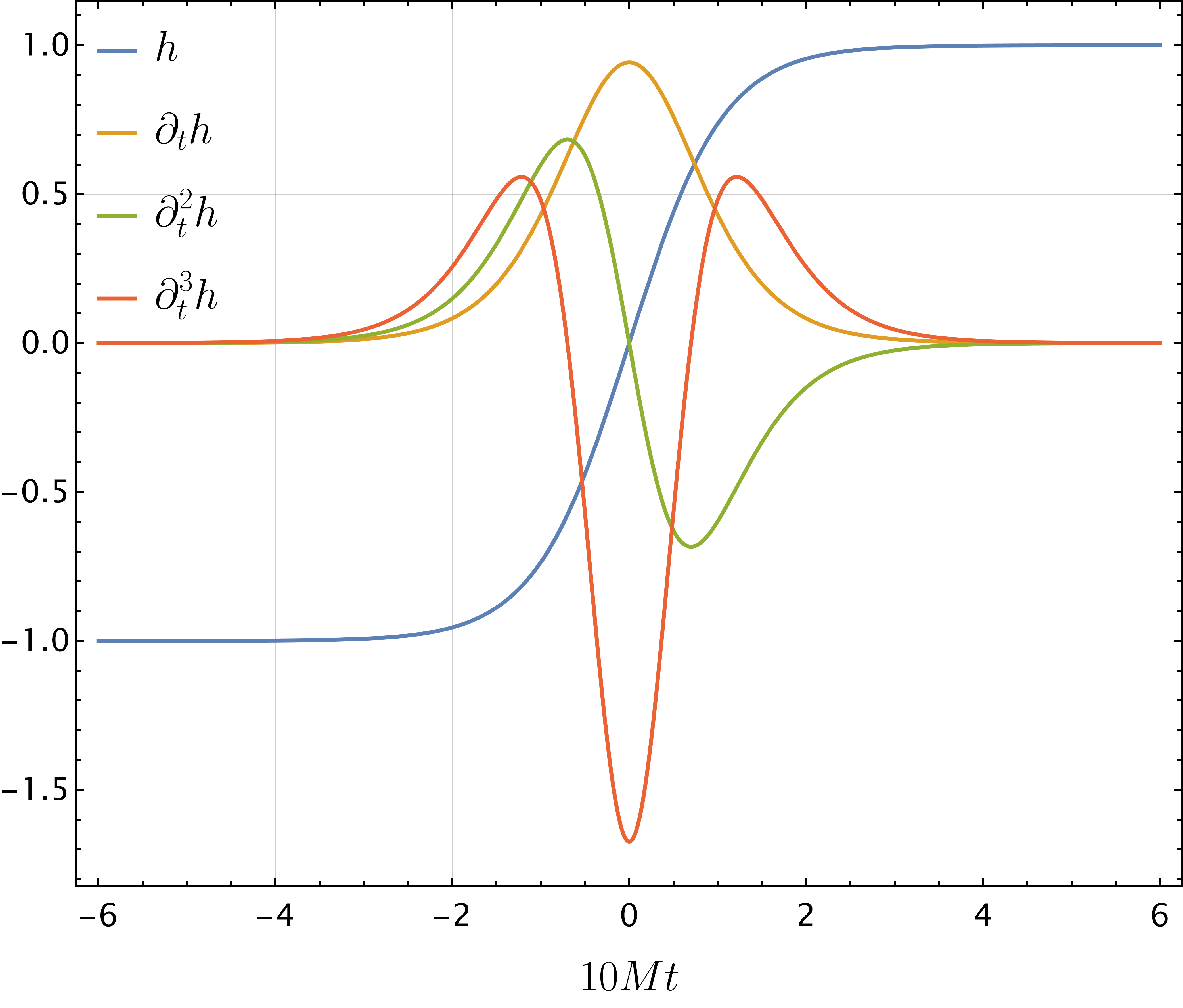
Going back to the step-like behavior of the memory signal, this can be approximated by a hyperbolic function with time raise , as explained in Section II,
| (17) |
with the merger time. We show this function in Figure 12 with its higher derivatives up to the third, noting that they all go to zero sufficiently far from the merger. In particular, note how the third derivative (red line) resembles the TDI result of the memory signal shown in Figure 2.
Appendix B Comparison of the memory between Surrogate_CCE and GWMemory package
As repeatedly discussed in the main text, we found some differences between the GW memory computed through Eq.(1), which subtracts the (2,0) mode of NRHybSur3dq8_CCE to that of NRHybSur3dq8_CCE, and using the GWMemory from the NRHybSur3dq8_CCE waveforms. The two differ by some oscillating features present in the first method compared to the second, as can be seen in Figure 13, where the smooth blue curve is the TDI of the memory calculated from GWMemory, while the red curve is calculated through Eq. (1). These oscillations are visible as small peaks in the power spectra of the signals shown in Figure 14, at frequencies higher than the typical frequencies of the memory. By comparing them with Figure 3 in the main text, one can see that they are just below the maximum frequency of the (2,2) mode of the primary signal. This might suggest that the discrepancy between the two has a physical origin that is better captured in the Numerical Relativity simulations. However, as mentioned in the text, the two waveforms used in Eq. (1) are not constructed exactly in the same way, then the comparison in Eq. (1) might not be robust in general, and can give rise to some numerical error, such as residual coming from the ringdown.

While rather small in the strain time-series (see left-hand side of 14), these high-frequency features are significantly magnified by the LISA response function, acting as a third-order high-pass filter (see right-hand plot of Figure 13). We find, however, that the discrepancy they occur do not impact sensibly SNR prospects for equal-mass sources, but have a stronger impact for higher (see Figure 10). Since, at this point, we cannot robustly identify the origin of such mismatch, we take a conservative approach and compute the SNR from the GWMemory when the mass ratio is which returns a more conservative value, and keep numerical relativity inherited NRHybSur3dq8_CCE evaluations for sources.

References
- Zel’dovich and Polnarev [1974] Y. B. Zel’dovich and A. G. Polnarev, Sov. Astron. 18, 17 (1974).
- Braginsky and Grishchuk [1985] V. B. Braginsky and L. P. Grishchuk, Sov. Phys. JETP 62, 427 (1985).
- Braginsky and Thorne [1987] V. B. Braginsky and K. S. Thorne, Nature (London) 327, 123 (1987).
- Christodoulou [1991] D. Christodoulou, Phys. Rev. Lett. 67, 1486 (1991).
- Flanagan et al. [2019] E. E. Flanagan, A. M. Grant, A. I. Harte, and D. A. Nichols, Phys. Rev. D 99, 084044 (2019).
- Grant and Nichols [2022] A. M. Grant and D. A. Nichols, Phys. Rev. D 105, 024056 (2022), [Erratum: Phys.Rev.D 107, 109902 (2023)].
- Grant and Nichols [2023] A. M. Grant and D. A. Nichols, Phys. Rev. D 107, 064056 (2023), [Erratum: Phys.Rev.D 108, 029901 (2023)].
- Siddhant et al. [2024] S. Siddhant, A. M. Grant, and D. A. Nichols, (2024).
- Pasterski et al. [2016] S. Pasterski, A. Strominger, and A. Zhiboedov, JHEP 12, 053 (2016).
- Nichols [2018] D. A. Nichols, Phys. Rev. D 98, 064032 (2018).
- Ashtekar et al. [2020] A. Ashtekar, T. De Lorenzo, and N. Khera, Gen. Rel. Grav. 52, 107 (2020).
- Mitman et al. [2024] K. Mitman et al., (2024).
- Strominger and Zhiboedov [2016] A. Strominger and A. Zhiboedov, JHEP 01, 086 (2016).
- Strominger [2017] A. Strominger, Lectures on the Infrared Structure of Gravity and Gauge Theory (2017).
- Bieri and Polnarev [2024] L. Bieri and A. Polnarev, Class. Quant. Grav. 41, 135012 (2024), arXiv:2402.02594 [gr-qc] .
- Payne [1983] P. N. Payne, Phys. Rev. D 28, 1894 (1983).
- Wiseman and Will [1991] A. G. Wiseman and C. M. Will, Phys. Rev. D 44, R2945 (1991).
- Blanchet and Damour [1992] L. Blanchet and T. Damour, Phys. Rev. D 46, 4304 (1992).
- Favata [2009a] M. Favata, Phys. Rev. D 80, 024002 (2009a).
- Blanchet et al. [2008] L. Blanchet, G. Faye, B. R. Iyer, and S. Sinha, Class. Quant. Grav. 25, 165003 (2008), [Erratum: Class.Quant.Grav. 29, 239501 (2012)].
- Favata [2010] M. Favata, Class. Quantum Gravity 27, 084036 (2010).
- Favata [2009b] M. Favata, The Astrophysical Journal 696, L159 (2009b), publisher: American Astronomical Society.
- Gasparotto et al. [2023] S. Gasparotto, R. Vicente, D. Blas, A. C. Jenkins, and E. Barausse, Physical Review D 107, 124033 (2023), publisher: American Physical Society.
- Xu et al. [2024] Y. Xu, M. Rosselló-Sastre, S. Tiwari, M. Ebersold, E. Z. Hamilton, C. García-Quirós, H. Estellés, and S. Husa, (2024).
- Tiwari et al. [2021] S. Tiwari, M. Ebersold, and E. Z. Hamilton, Phys. Rev. D 104, 123024 (2021).
- Lopez et al. [2024] D. Lopez, S. Tiwari, and M. Ebersold, Phys. Rev. D 109, 043039 (2024).
- Goncharov et al. [2023] B. Goncharov, L. Donnay, and J. Harms, (2023).
- Heisenberg [2023] L. Heisenberg, Philosophical Transactions of the Royal Society A: Mathematical, Physical and Engineering Sciences 382, 20230086 (2023), publisher: Royal Society.
- D’Ambrosio et al. [2024] F. D’Ambrosio, F. Gozzini, L. Heisenberg, H. Inchauspé, D. Maibach, and J. Zosso, “Testing gravitational waveforms in full General Relativity,” (2024), arXiv:2402.19397 null.
- Du and Nishizawa [2016] S. M. Du and A. Nishizawa, Phys. Rev. D 94, 104063 (2016).
- Tahura et al. [2021] S. Tahura, D. A. Nichols, and K. Yagi, Phys. Rev. D 104, 104010 (2021).
- Heisenberg et al. [2023a] L. Heisenberg, N. Yunes, and J. Zosso, Phys. Rev. D 108, 024010 (2023a).
- Heisenberg et al. [2024] L. Heisenberg, G. Xu, and J. Zosso, (2024).
- McNeill et al. [2017] L. O. McNeill, E. Thrane, and P. D. Lasky, Phys. Rev. Lett. 118, 181103 (2017).
- Ghosh et al. [2023] S. Ghosh, A. Weaver, J. Sanjuan, P. Fulda, and G. Mueller, Phys. Rev. D 107, 084051 (2023).
- Hübner et al. [2020] M. Hübner, C. Talbot, P. D. Lasky, and E. Thrane, Phys. Rev. D 101, 023011 (2020).
- Ebersold and Tiwari [2020] M. Ebersold and S. Tiwari, Phys. Rev. D 101, 104041 (2020).
- Zhao et al. [2021] Z.-C. Zhao, X. Liu, Z. Cao, and X. He, Phys. Rev. D 104, 064056 (2021).
- Hübner et al. [2021] M. Hübner, P. Lasky, and E. Thrane, Phys. Rev. D 104, 023004 (2021).
- Seto [2009] N. Seto, Mon. Not. Roy. Astron. Soc. 400, L38 (2009).
- Cordes and Jenet [2012] J. M. Cordes and F. A. Jenet, Astrophys. J. 752, 54 (2012).
- Agazie et al. [2024] G. Agazie et al., Astrophys. J. 963, 61 (2024).
- Punturo et al. [2010] M. Punturo et al., Class. Quant. Grav. 27, 194002 (2010).
- Reitze et al. [2019] D. Reitze et al., Bull. Am. Astron. Soc. 51, 035 (2019).
- Favata [2009c] M. Favata, Astrophys. J. Lett. 696, L159 (2009c).
- Johnson et al. [2019] A. D. Johnson, S. J. Kapadia, A. Osborne, A. Hixon, and D. Kennefick, Phys. Rev. D 99, 044045 (2019).
- Islo et al. [2019] K. Islo, J. Simon, S. Burke-Spolaor, and X. Siemens, (2019).
- Islam et al. [2021] T. Islam, S. E. Field, G. Khanna, and N. Warburton, (2021).
- Sun et al. [2022] S. Sun, C. Shi, J.-d. Zhang, and J. Mei, (2022).
- Sun et al. [2024] S. Sun, C. Shi, J.-d. Zhang, and J. Mei, (2024).
- van Haasteren and Levin [2010] R. van Haasteren and Y. Levin, Mon. Not. Roy. Astron. Soc. 401, 2372 (2010).
- Janssen et al. [2015] G. Janssen et al., PoS AASKA14, 037 (2015).
- Yoo et al. [2023] J. Yoo, K. Mitman, V. Varma, M. Boyle, S. E. Field, N. Deppe, F. Hébert, L. E. Kidder, J. Moxon, H. P. Pfeiffer, M. A. Scheel, L. C. Stein, S. A. Teukolsky, W. Throwe, and N. L. Vu, Physical Review D 108, 064027 (2023), publisher: American Physical Society.
- Barausse and Lapi [2020] E. Barausse and A. Lapi, (2020).
- Barausse et al. [2020] E. Barausse, I. Dvorkin, M. Tremmel, M. Volonteri, and M. Bonetti, Astrophys. J. 904, 16 (2020).
- Barausse [2012] E. Barausse, Mon. Not. Roy. Astron. Soc. 423, 2533 (2012).
- Sesana et al. [2014] A. Sesana, E. Barausse, M. Dotti, and E. M. Rossi, Astrophys. J. 794, 104 (2014).
- Antonini et al. [2015] F. Antonini, E. Barausse, and J. Silk, Astrophys. J. 812, 72 (2015).
- Colpi et al. [2024] M. Colpi et al., “LISA Definition Study Report,” (2024), arXiv:2402.07571 [astro-ph, physics:gr-qc].
- Bayle et al. [2023a] J.-B. Bayle, Q. Baghi, A. Renzini, and M. Le Jeune, “LISA GW Response,” (2023a), language: eng.
- Bayle et al. [2022] J.-B. Bayle, A. Hees, M. Lilley, and C. Le Poncin-Lafitte, “LISA Orbits,” (2022), language: eng.
- Bayle and Hartwig [2023] J.-B. Bayle and O. Hartwig, Physical Review D 107, 083019 (2023), publisher: American Physical Society.
- Bayle et al. [2023b] J.-B. Bayle, O. Hartwig, and M. Staab, “LISA Instrument,” (2023b).
- Staab et al. [2023] M. Staab, J.-B. Bayle, and O. Hartwig, “PyTDI,” (2023), language: eng.
- Handmer et al. [2016] C. J. Handmer, B. Szilágyi, and J. Winicour, Class. Quant. Grav. 33, 225007 (2016).
- Mitman et al. [2020] K. Mitman, J. Moxon, M. A. Scheel, S. A. Teukolsky, M. Boyle, N. Deppe, L. E. Kidder, and W. Throwe, Phys. Rev. D 102, 104007 (2020).
- Favata [2009d] M. Favata, Journal of Physics: Conference Series 154, 012043 (2009d).
- Talbot et al. [2018a] C. Talbot, E. Thrane, P. D. Lasky, and F. Lin, Phys. Rev. D 98, 064031 (2018a).
- Khera et al. [2021] N. Khera, B. Krishnan, A. Ashtekar, and T. De Lorenzo, Phys. Rev. D 103, 044012 (2021).
- Mitman et al. [2021] K. Mitman et al., Phys. Rev. D 103, 024031 (2021).
- Rosselló-Sastre et al. [2024] M. Rosselló-Sastre, S. Husa, and S. Bera, (2024).
- Varma et al. [2019] V. Varma, S. E. Field, M. A. Scheel, J. Blackman, L. E. Kidder, and H. P. Pfeiffer, Physical Review D 99, 064045 (2019), publisher: American Physical Society.
- Thorne [1992] K. S. Thorne, Phys. Rev. D 45, 520 (1992).
- Baghi et al. [2023] Q. Baghi, N. Karnesis, J.-B. Bayle, M. Besançon, and H. Inchauspé, Journal of Cosmology and Astroparticle Physics 2023, 066 (2023), publisher: IOP Publishing.
- Heisenberg et al. [2023b] L. Heisenberg, H. Inchauspé, D. Q. Nam, O. Sauter, R. Waibel, and P. Wass, Physical Review D 108, 122007 (2023b), publisher: American Physical Society.
- Tinto and Dhurandhar [2020] M. Tinto and S. V. Dhurandhar, Living Reviews in Relativity 24, 1 (2020).
- Vallisneri [2005] M. Vallisneri, Physical Review D 72, 042003 (2005), publisher: American Physical Society.
- Boyle et al. [2019] M. Boyle et al., Classical and Quantum Gravity 36, 195006 (2019), publisher: IOP Publishing.
- McKechan et al. [2010] D. J. A. McKechan, C. Robinson, and B. S. Sathyaprakash, Classical and Quantum Gravity 27, 084020 (2010).
- Team [2018] L. S. S. Team, Science Requirement Document, Tech. Rep. ESA-L3-EST-SCI-RS-001 (2018).
- Quang Nam et al. [2023] D. Quang Nam, J. Martino, Y. Lemière, A. Petiteau, J.-B. Bayle, O. Hartwig, and M. Staab, Physical Review D 108, 082004 (2023), publisher: American Physical Society.
- Pitte et al. [2023a] C. Pitte, Q. Baghi, S. Marsat, M. Besançon, and A. Petiteau, Physical Review D 108, 044053 (2023a), publisher: American Physical Society.
- Babak et al. [2021a] S. Babak, M. Hewitson, and A. Petiteau, “LISA Sensitivity and SNR Calculations,” (2021a), arXiv:2108.01167 [astro-ph, physics:gr-qc].
- Babak et al. [2021b] S. Babak, A. Petiteau, and M. Hewitson, (2021b).
- Buonanno et al. [2007] A. Buonanno, G. B. Cook, and F. Pretorius, Phys. Rev. D 75, 124018 (2007).
- Chen et al. [2024] Y. Chen et al., (2024).
- Zonca et al. [2019] A. Zonca, L. P. Singer, D. Lenz, M. Reinecke, C. Rosset, E. Hivon, and K. M. Gorski, Journal of Open Source Software 4, 1298 (2019).
- Górski et al. [2005] K. M. Górski, E. Hivon, A. J. Banday, B. D. Wandelt, F. K. Hansen, M. Reinecke, and M. Bartelmann, The Astrophysical Journal 622, 759 (2005), publisher: IOP Publishing.
- Pitte et al. [2023b] C. Pitte, Q. Baghi, S. Marsat, M. Besançon, and A. Petiteau, Phys. Rev. D 108, 044053 (2023b).
- Talbot et al. [2018b] C. Talbot, E. Thrane, P. D. Lasky, and F. Lin, Physical Review D 98, 064031 (2018b), publisher: American Physical Society.
- Liu et al. [2021] X. Liu, X. He, and Z. Cao, Phys. Rev. D 103, 043005 (2021).
- Cao and Han [2016] Z. Cao and W.-B. Han, Classical and Quantum Gravity 33, 155011 (2016).
- Pollney and Reisswig [2011] D. Pollney and C. Reisswig, Astrophys. J. Lett. 732, L13 (2011).
- Barausse et al. [2023] E. Barausse, K. Dey, M. Crisostomi, A. Panayada, S. Marsat, and S. Basak, Phys. Rev. D 108, 103034 (2023).
- García-Quirós et al. [2020] C. García-Quirós, M. Colleoni, S. Husa, H. Estellés, G. Pratten, A. Ramos-Buades, M. Mateu-Lucena, and R. Jaume, Physical Review D 102, 064002 (2020), publisher: American Physical Society.
- Caldarola et al. [2024] M. Caldarola, S. Kuroyanagi, S. Nesseris, and J. Garcia-Bellido, Phys. Rev. D 109, 064001 (2024).
- Gröbner et al. [2020] M. Gröbner, W. Ishibashi, S. Tiwari, M. Haney, and P. Jetzer, Astron. Astrophys. 638, A119 (2020), arXiv:2005.03571 [astro-ph.GA] .
- Dandapat et al. [2023] S. Dandapat, M. Ebersold, A. Susobhanan, P. Rana, A. Gopakumar, S. Tiwari, M. Haney, H. M. Lee, and N. Kolhe, Phys. Rev. D 108, 024013 (2023), arXiv:2305.19318 [gr-qc] .
