How & Why to Use Audience Segmentation
to Maximize (Listener) Demand
Across a Digital (Music) Portfolio
Abstract.
Digital delivery of songs has radically changed the way people can enjoy music, the sort of music available for listening, and the manner by which rights holders are compensated for their contributions to songs. Listeners enjoy an unlimited potpourri of sounds, uniquely free of incremental acquisition or switching costs which have been replaced by subscription or rentier fees. This regime shift has revealed listening patterns governed by affinity, boredom, attention budget, etc.: instantaneous, dynamic, organic or programmatic song selection. This regime shift in demand availability - with the commensurate translation of revenue implications - deprecates current orthodoxy for content curation. The impulse to point-of-sale model is insufficient in a regime where demand revenue is proportional to demand affinity and each are strongly dependent time series processes. We explore strategies & implications - which are generalizable to any media rights holding firm - from a prediction & optimization point of view for two straightforward demand models.
1. A Simple Dynamic Model for Streaming Song Listening
This paper focuses on modeling demand for a ’song’ - generally a two to five minute musical composition - consumable via some digital delivery service or Digital Streaming Provider (DSP) and strategic, macroscopic, inferences that may be deduced from an elucidation of some assumptions around the demand for those songs.
Nile Rodgers, in an interview about his influence on popular music of the 1970’s and 1980’s recalled this exchange with Miles Davis:
Miles would always ask me to make him a hit like how I did for [David] Bowie. I never took him seriously until he covered [Cyndi Lauper’s] ‘Time after Time.’ I listened to that track and realized he was serious, and like most artists, wanted as many people to hear him as possible. [15]
This paper addresses macroscopic dynamics of song listening, via model eludcidation of idiosyncratic, dynamic or microscopic listener group-by-listener group differences. That is, we focus on the aggregate demand dynamics of a population, or sub-population, enjoying a ’song’ as a function of time, aggregating (if not fully eliding) the individual or group-wise ’utilities’ – here probability of listening – into larger group-wise aggregate demand.
1.1. Streaming Demand as a Counting Process
To begin, but without loss of generality, we consider a ’song’ a de novo offering: a new, or new version of a composition yielding a demand curve with a fixed point at (0,0): time zero, just as a song is released - or, in the parlance, dropped.
In similarity with [7], the model for volume of listening, or listener response to a listening ’opportunity’, is a counting process where any individual listener enjoys a song with a (not-necessarily) time variant probability 111In this paper capital letters represent random processes, lower case letters observed or observable values. We rely on the random processes as U-statistics [6] for measurability, and other, assumptions.:
| (1) |
This models the time dependent aggregated listening (as an affinity curve, say – an aggregation of individual observed utilities for listeners) as demand curves:
| (2) |
the cumulation of individual listening demand within each listening strata, , yielding a song-level demand curve.
| (3) |
indexes the collection of listener strata and may coincide, or not, with the categorically defined DSPs.222The collection of listening strata (in an abuse of notation used for both the stratum and its cardinality) are not necessarily disjoint. These curves are models for listener preference, over time, for coherent - but not necessarily identical - patterns of listening demand or consumption unique to the ’listening mode.’ A ’listening mode’ can be as idiosyncratic as the set of rules (or some of the set of rules) which increment a song as a fully ’listened to’ stream on a particular DSP (30 seconds of listening, say, on a particular provider), or as collective as merely on which DSP a song is enjoyed.
Our model is an extension of the well-known ‘DSP-wise’ differences in listening affinity to more general segmentation of listening affinities. One way to convey this is to say that any listener, at any time, may be exposed to (and listen to) any song for any reason - in fact, multiple reasons.
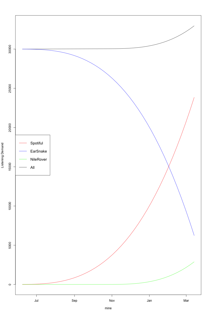
In Figure 1 a cartoon graphic of listening demand for a song for a 40 week interval: the height of each curve is the number of listeners within each week on each DSP, say; each colored curve aggregates listeners for a unique subscription service within each week. The black curve is the total from each and the overall demand curve. This illustration should be familiar to music industry executives and/or artists: an important heuristic for modeling song performance is that it should be clear that a song performs differentially (over time) on different platforms. DSPs can appeal to different audiences, with possibly different listening preferences; each DSP may offer variegated subscription plans, which may appeal to listening preferences heterogenously.
The aggregate curve in Figure 1 – in black at the top – conveys a slow steady growth in listening demand. The other curves, on audience (sub) segments illustrate the differential listener affinities (at least, on different DSPs). This sort of rich, differential, picture of demand that is invaluable to a modern content rights holder.
1.2. Other Counting Process for Streaming Demand
Content rights holders typically receive intermediated information on listener demand, via the DSPs, in a way that is similar to data scientists in advertising technology. To account for this ’schmutzdecke’333From my past as an environmental statistician we augment the naive observed data models with processes offered by latent or hidden features. Let
| (4) |
a boundary process, on the best possible audience strata – i.e. with maximum listening affinity. And let
| (5) |
be the lower boundary.
Content rights holders are concerned with song performance – and the ability to characterize a song’s performance – in the presence of confounding factors: temporality, ambient head or tailwinds, DSP idiosyncrasy, bad luck, etc. There are many hard to quantify explanations for song performance. Fixing and as the extremal demand processes, with respect to the process model, can yields stable comparative models for performance characteristics.

1.3. Model for Listener Affinity
The model for listener affinity is
| (6) | ||||
| (7) |
Remember that the individual listening affinities are collected within listening strata , which are arbitrarily coherent, but not necessarily disjoint groups such that
| (8) |
the listening curve can be modeled as from an individual listener or, say, where modeling all the listener demand, at a particular ratecarding at a DSP, as equivalent as from one or a few audience strata. Covariates for exogenous or ambient effects on demand are collected in ; those for endogenous effects (marketing, complementary media, social media, etc.) are collected in . Assume the and dimensional covariates are non-negative such that: .
1.4. Song Demand via Listening Mode
Figure 3 is a plot and characterization of observed demand curves for 1,000 de novo songs, with demand curves observed in calendar year 2021, on a popular streaming service. The demand curves were classified by k (=7) mean classification via the Python tslearn toolkit to illustrate differences in song demand curves.

Figure 3 points to varied modes for listening and song demand: song demand peaks and decays with regular, differentiable characters. Modeling the incidental processes through to the extremal process curves, lets the model be flexible for the available data granularity.
1.5. The importance of audience segmentation
A feature of this model is to be able to model listening affinity/utility as i.i.d within audience segment. Let audience segments be a covering s.t
| (9) | ||||
One can think of an audience segment as a listening group which responds similarly to listening stimuli (at a particular time); within each segment we model the utilities as i.i.d. - random but identically distributed. The are non-disjoint because individual listeners may occupy more than one utility for listening (at a particular time) a particular song.444N.B. that the time index for streaming demand modeling can be coarse, where each increment is one week. The ability to segregate demand to unique audience segments and model differences in effects is important. Let
| (10) |
be the ‘sparse’ audience: , with the symmetric difference operator.
Contemporary work on streaming demand ([7], [12]) elides listener level utility with aggregation, perhaps as user level data are hard to come by. The audience segmentation device in this paper joins varied hierarchical level listening demand data with listener level utility models ([16], [18]). This resonates with the both the spirit of ([2]) and the similarities in theoretical process models they derive and both they and we observe in data.
2. Covariate Models for Processes & Forecasting
Within any coherent audience segment the affinity
| (11) |
can exploit models for binary processes: here we can write and use the estimators for the segment-wise affinities via a logistic model. Straightaway the estimators for effects of ambient or () covariates () or the effects () of business levers () can be modeled using individual, user level data – if available. Where these data aren’t available – for example Apple Music’s API does not offer granular, user level data – we can use segment-wise counts and covariates and then we can appeal to natural counting process models, for these aggregates. For example, for observed demand curve , for audience segment , the distribution of the size of the audience strata is:
| (12) |
The Negative Binomial distribution relates the demand curves’ observed value, to the size of the listening strata in terms of the covariates as is covariate dependent. More straightforwardly Poisson or Negative Binomial regression can as well specify the effects of the covariates on the demand curves:
| (13) |
and control charts for covariate effects can be easily generated with
| (14) |
as conditional demand curves given proposed ambient or endogenous predictors.
2.1. Fully Bayesian Workflow for Streaming Demand
Here it is important to invoke a modeling perquisite: translating the songs to a time-demand interval beginning at . This condition is met if data for release dates and listening demand beginning from release are available. This condition though is not always necessary, nor it is necessarily sufficient. Consider a model forecasting demand behavior for a song in deep catalog: a song that was released many years ago. We illustrated in Figs. 1-3 the growth-decay character of listening demand for de novo songs; these demand patterns may exist within several alternate or similar periodic behaviors.
For example, when an audience segment of young listeners discover Stevie Wonder: the mode of growth and decay of listening can be similar, for this strata, to a new release. A forecaster who wants to consider aggregate future demand for a re-release of Stevie’s Jesus Children of America, say, can’t rely fully on only the dynamics of de novo songs by comparable artists or even Stevie Wonder himself but within strata the assumption is tenable and across stratum models are fit on the convolution.
A fully Bayesian setup [4] for collecting, training, estimating and updating the model(s) for streaming demand co-ordinates demand response, covariate information and metadata in a framework that is useful for monitoring and gauging song performance in-the-moment and as well yields a full-distributional tableau for a subsequent optimization scheme.

Null Model
| (15) | ||||
Figure (5) elucidates a Bayesian model which captures listener stratum and artist level effects - accounting for differences in utility, say, among the effects on listeners who enjoy only the unique rhythm gbitar, organ and synthesizer on the Ohio Players’ single Ecstasy and those who have an ear for it in the rest of the album. This hierarchy can of course be extended. Notice that this model is forced by the effect of ambient and planned actions as realized upon listener stratum. These effects in this model are time-invariant and the model itself only accounts for time dependent effects via the value of the predictor processes. This model, thusly, does not necessarily yield a growth-decay process, but for the observed values of the covariate forcings and/or migration out of high affinity (and thus positive estimated effect) listener segments. One can imagine an affinity process where covariate forcing continues at a constant level - especially given the model’s partition of listeners into non-disjoint strata. But there is only one Bob Marley.555Or Michael Jackson, or Jan Hammer, or KraftWerk.
The model in Figure (7) fixes growth-decay conditions on the listener segment counting processes. In this version of the model the main effects estimators, for the utility forcings, are estimated as projection on subspaces of a phase transition model and in this way mediated or attenuated depending upon the phase of the process. One reason for not treating this as a fully Gaussian Process with a Latent Variable ([10]) is that the generating processes here are only Gaussian in a large numbers regime. Starting from first principles here yields distributional inference even for songs and artists that are less popular, i.e. that stretch the Gaussian assumption on the feature space. The specification of model phase conditional on the estimated change points is equivalent to assuming the main effects estimators within each phase are independent with respect the other phases; that the estimators in each phase are projected away from the ancillary subspaces - the other phases ([9], [3]).666In practice it is desirable to estimate the change points separately and first. The model estimates a subspace for each phase of the process; the effects (ambient and endogenous forcing of the listener segment utilities) estimators are conditional on each estimated subspace. Estimating the phases first can be a common sense check before embarking on the full posterior. This is addressed this again below.
3. Conditions for and on Streaming Demand
Recall that is the total audience available for a song; fix it constant for each time over the period ; usually quite large, each often a week.. Recall that the form a non-disjoint covering for s.t. individual listeners may be in more than one audience segment (at a time) . The audience segment covering permits differential response to marketing strategies , say, and ambient events that affect listening affinity – within each equal time interval – via effects and . Conversationally, the audience segment covering conveys the audience segment-wise reason at a particular time for listening: one time during exercise, another time in an algorithmic playlist of new songs, another time to prepare for sleeping.
This model places any budget for listening – from the perspective of the listener – as a function of the utility curves’ response to marketing or ambient impulses – i.e. the magnitude of the coefficients and – and models incremental listening as membership in a different audience segment (e.g. listeners’ ability to listen for a different reason).777This is an important distinction between the song and utility of listening it at a particular time, for a particular reason. From the perspective of the listener this a model for listening choices; from the perspective of the inventory holder (song creator or curator) its a model for song demand. The impacts of endogenous & exogenous forcings are conveyed via the individual listening utilities, i.e. realized probabilities.
3.1. Null Model
Consider the maximization of listening under the null model, where the sole dynamic is listener affinity. From equation (6) the user level utility curves are a function of endogenous and exogenous dynamics via effects, respectively – i.e. spend per marketing channel, impulse per social channel, demand per marketing spend and demand per social channel.
Let the endogenous budget (the amount of money the rights holder has to spend through ) for a song be:
| (16) | ||||
with a vector of ones the same length as . This is just to say that the rights holder has a finite & necessarily and wholly exhaustible budget for endogenous forcing.
Maximization of Null Model
| (17) | ||||
A program for the maximization of expected utility for a listener within a particular segment at time window is in figure (17). Notice that the utility maximization within each listening segment is equivalent to probability maximization within segment. The maximal input for the path, as a function of time, is derived from the Lagrangian for the optimization scheme in (17):
| (18) |
where is a vector pseudo-inverse. This is to take the maximum of either the scaled available budget , or the scaled residue beyond the endogenous effects ; each ’scaled’ by the relative effect of endogenous - or business-wise levers - on the song utility, within each audience segment. In practice the budget can be reallocated across audience segments - and it should be - to follow the (estimated) effect for greatest gain in audience magnitude.
3.2. ADSR/Forcing Model
Forced (envelope) Model
| (19) |
The forced model imposes a pattern, or a template of, overarching listening affinity (or song uptake). Refer again to Figure 3. The use of the forcing model is to exploit the regular patterns in aggregate song demand with a model that reduces the inference burden while increasing the explanatory power. Here, we use the envelope model – common to the sound engineering literature as a model for the intensity of a sound over time [14], and a well-known generative tool for modifying a sound. Statistically this model is a special case of a phase transition model (see [5]) - characterized by discontinuities between the phases at the transitions. Referring to the elucidation in equation (7) this model is fit in two steps:
- I
-
II
Fit the partite models Each phase of the ADSR model is essentially linear: the parameters to be fit are the slopes and intercepts for each linear part; the effects between the endogenous and exogenous covariates; the distributional hyperparameters for dependency between and precision of those effects.
The model is conceived to capture dynamics for de novo songs - songs new to an audience of listeners,888To borrow jargon from advertising technology, the in-flight period for an advertisement is the length of time an advert is placed within media for impressions. yet is flexible to serve for songs with varied observed release times and listener exposure.
In the forcing model the endogenous and exogenous effects are estimated jointly with the partite linear model parameters. This is simply to say that the model flexibly estimates the effect on listener affinity within audience segment and subject to the growth/decay phase of the song, given the ADSR model.
The equations in (7) & (8) now specify a Bayesian hierarchy similar to the unforced model but with estimators for effects that are constant within phase. This simplifies the maximization scheme. For example, in phase the maximum expectation is at time , within this phase the estimating equations for effect are & . The mean value function in this phase, is defined as in the unforced model.
Maximization of Forcing Model, at phase extrema
| (20) | ||||


4. Comments and Recommendations
Either of these models should ‘fit’ nicely within current rights holder management schemes. Either model can be dynamically instantiated - in particular the phased/forcing model - with a simple LP. The forcing model needs only (linear) estimators for the mean value function at the change of phase after the change points themselves are estimated. Knowledge of these estimators - especially for this model - make a straightforward optimal path for listening maximization.
Time scales for marketing in aural media are discrete. Typically song performance is evaluated from week-to-week; advertising & social campaigns can be adjusted weekly. Optimization schemes work well on a portfolio of assets. Use of either version of these models on a suite of assets is preferable. It is conceivable that estimators for marketing or ambient effects on listening affinity trade or switch magnitude and sign across time periods, e.g. Halloween music, Christmas music.
An innovation shared by both the null and forcing models is to simply be willing to segregate the sources of (listening) demand and keep track of the marketing actions within each segment to yield usable time-aware effect estimators. Zooming out: audience segmentation for listening demand is key, perhaps even more for sound media demand than visual. It is not much to measure differential effects of marketing & exposure to a sound once it is observed the same song is listened to by different audiences in different ways at different times, etc.
5. Acknowledgment.
The author wishes to thank his colleagues at Seton Hall University and the many hardworking data and sound scientist friends he made at Warner Music Group & Warner Media, in particular Daniel Lee who discovered the envelope model for this use and Julien DeMori for his guidance on sound. An additional thanks to Yifeng Yu of the Music Information Program (led by Alexander Lerch) whose collaboration appears in a sequel to this paper. The author dedicates this paper to his father, Atiim Abayomi, who shared his love of music openly and who is sorely missed.
References
- [1] Barr, Donald R. & Sherrill, E. Todd ”Mean and Variance of Truncated Normal Distributions.” The American Statistician 53, 4. pp. 357-361
- [2] C. Candia, C. Jara-Figueroa, C. Rodriguez-Sickert, A Barabási, & C. Hidalgo. The universal decay of collective memory and attention. Nature Human Behavior. 3:January 2019. 82-91.
- [3] C Cook. An Introduction to Envelopes: Dimension Reduction for Efficient Estimation in Multivariate Statistics. Hoboken, NJ: John Wiley & Sons.
- [4] A. Gelman, J. Carlin, H. Stern, D. Dunson, A. Vehtari, & D. Rubin. Bayesian Data Analysis. CRC Press, Third Edition.
- [5] Gomez H, Bures M, Moure A. 2019 A review on computational modelling of phase-transition problems. Phil. Trans. R. Soc. A 377:2018, 0203.
- [6] W. Hoeffding Probability Inequalities for Sums of Bounded Random Variables. Ph.D. thesis, University of North Carolina Department of Statistics. May 1962.
- [7] Ivaldi M., Nicolle A., Verboven F., & Zhang J. Displacement and complementarity in the recorded music industry: evidence from France. Journal of Cultural Economics Feb 2023.
- [8] Koop G. & Potter. S. Prior Elicitation in Multiple Change-Point Models. International Economic Review Aug 2009. 30, 3:pp 751-772.
- [9] Li, B. & Song, J. (2017). Nonlinear sufficient dimension reduction for functional data. The Annals of Statistics, 45(3):1059–1095.
- [10] Li P. & Chen S. A Review on Gaussian Latent Process Models. CAAI Transactions on Information Technology. 1. 2016. pp. 366-376.
- [11] D. Lewandoski, D. Kurowicka, & H. Joe. Generating random correlation matrices based on vines and extended onion method. Journal of Multivariate Analysis. Elsevier, 200, Vol 100, Issue 9, pp. 1989-2001
- [12] A. Ordanini, J. Nunes, & A. Nanni. The featuring phenomenon in music: how combining artists of different genres increases a song’s popularity. Marketing Letters 2018. 29:485-499
- [13] Polunchencko A., Tartovsky A. State of the Art in Sequential Change Point Detection. Methodol Comput Appl Probab (2012) 14:649–684
- [14] Puckett, M. The Theory and Technique of Electronic Music. World Scientific Publishing Company. August 2007.
- [15] Diggin’ In The Crates With Nile Rodgers. Season 4, Episode 8. Available at https://www.youtube.com/watch?v=Uy70I5KbHno
- [16] K. Tam, W. vanTilburg, C. Chan, E. Igou, & H. Lau The Boredom Feedback Model. Personality and Social Psychology Review 25, 3.
- [17] F. Petitjean, A. Ketterlin & P. Gancarski. A global averaging method for dynamic time warping, with applications to clustering. Pattern Recognition, Elsevier, 2011, Vol. 44, Num. 3, pp. 678-693
- [18] Z. Wojtowicz, N. Chater, & G.F. Loewenstein, Boredom and Flow: An Opportunity Cost Theory of Motivational Attention (March 13, 2019). Available at SSRN: https://ssrn.com/abstract=3339123 or http://dx.doi.org/10.2139/ssrn.3339123
