A space-time variational formulation for the many-body electronic Schrödinger evolution equation

Mi-Song Dupuy, Virginie Ehrlacher, Clément Guillot

Abstract

We prove in this paper that the solution of the time-dependent Schrödinger equation can be expressed as the solution of a global space-time quadratic minimization problem that is amenable to Galerkin time-space discretization schemes, using an appropriate least-square formulation. The present analysis can be applied to the electronic many-body time-dependent Schrödinger equation with an arbitrary number of electrons and interaction potentials with Coulomb singularities. We motivate the interest of the present approach with two goals: first, the design of Galerkin space-time discretization methods; second, the definition of dynamical low-rank approximations following a variational principle different from the classical Dirac-Frenkel principle, and for which it is possible to prove the global-in-time existence of solutions.

Statements and Declarations: This publication is part of a project that has received funding from the European Research Council (ERC) under the European Union’s Horizon 2020 Research and Innovation Programme – Grant Agreement 101077204.

1 Introduction

The aim of this paper is to introduce a new global space-time variational formulation of the linear evolution Schrödinger equation

\begin{cases}(i\partial_{t}-H-B(t))u^{*}(t)=f(t),\quad t\in I\\ u^{*}(0)=u_{0},\end{cases}

(1)

where $H$ is a self-adjoint operator on a separable Hilbert space $\mathcal{H}$ with domain $D\!\left(H\right)$ , $I=(0,T)$ for some $T>0$ and $B:\overline{I}\ni t\mapsto B(t)$ is a strongly continuous family of bounded self-adjoint operators on $\mathcal{H}$ . The general setting above includes the case of the time-dependent Schrödinger equation defined on the whole space (in arbitrary large dimension) and with interaction potential with Coulomb singularities. This includes in particular the case of the time-dependent Schrödinger evolution equation associated to the many-body electronic Hamiltonian for molecules. The latter concerns the following case: consider a system of $N\in\mathbb{N}^{*}$ electrons in a molecule with $M\in\mathbb{N}^{*}$ nuclei in the Born-Oppenheimer approximation. Let us assume that the positions and electric charges of the nuclei are given respectively as $R_{1},\ldots,R_{M}\in\mathbb{R}^{3}$ and $Z_{1},\ldots,Z_{M}>0$ . Then, $\mathcal{H}=L^{2}(\mathbb{R}^{3N})$ (or $\mathcal{H}=\bigwedge_{i=1}^{N}L^{2}(\mathbb{R}^{3})$ the set of antisymmetric functions of $L^{2}(\mathbb{R}^{3N})$ ) and $H=-\Delta-\sum_{k=1}^{M}\sum_{i=1}^{N}\frac{Z_{k}}{|x_{i}-R_{k}|}+\sum_{1\leq i<j\leq N}\frac{1}{|x_{i}-x_{j}|}$ , the quantity $|\cdot|$ denoting the euclidean norm in $\mathbb{R}^{3}$ .

The goal of the present work is to reformulate the solution $u^{*}$ of (4) as the unique solution of a minimization problem of the form

\text{Find $u^{*}\in\mathcal{X}_{H}$ such that}\;u^{*}=\operatorname*{argmin}_{u\in\mathcal{X}_{H}}E(u)

(2)

with $\mathcal{X}_{H}$ a suitable Hilbert space and $E$ is the quadratic (strongly convex) functional associated to the Lax-Milgram variational problem

\forall u\in\mathcal{X}_{H},\quad a(u^{*},u)=l(u)

where $a:\mathcal{X}_{H}\times\mathcal{X}_{H}\to\mathbb{C}$ is a continuous hermitian coercive sesquilinear form on $\mathcal{X}_{H}\times\mathcal{X}_{H}$ and $l:\mathcal{X}_{H}\to\mathbb{R}$ is a continuous linear form. More precisely, we introduce an appropriate least-square formulation [6] of the latter equation.

Under suitable assumptions on the Hamiltonian $H$ , there are many such possible variational formulations. The wish list that we have in mind to pick an appropriate variational formulation is the following:

(i)

the coercivity and continuity constants of the bilinear form $a$ should not decrease (respectively increase) too fast with the value of the final time $T$ ;
(ii)

it should yield practical Galerkin space-time numerical schemes;
(iii)

it should be useful to define new dynamical low-rank approximations using a different variational principle than the classical Dirac-Frenkel principle [18, 17, 16, 2, 7, 1]. The advantage of the proposed formulation is that it is possible then to prove the global-in-time existence of some dynamical low-rank approximations, without any restrictions on the data of the problem.

The variational formulation presented in this work satisfies these three requirements, as will be explained in the article. We would like to stress on the fact that our present analysis covers the case of unbounded domains and interaction potentials with Coulomb singularities, which includes the case of the many-body electronic Schrödinger Hamiltonian introduced above. While our main motivation for the present work stems from the design of new global-in-time dynamical low-rank approximations, which will be the object of another forthcoming article, we present here some preliminary numerical results about global space-time Galerkin discretization schemes for the time-dependent Schrödinger equation associated to the variational formulation we present here.

Let us thus comment here about the state-of-the-art of global space-time discretization methods for the time-dependent Schrödinger equation. In [5], a spacetime discontinuous Petrov-Galerkin (DPG) method for the linear time-dependent Schrödinger equation is proposed. Two variational formulations are proved to be well posed: a strong formulation (with no relaxation of the original equation) and a weak formulation (also called the “ultraweak formulation,” which transfers all derivatives onto test functions). However, the analysis is restricted to the case of an equation posed on a bounded domain and without an interaction potential. In [8] and [9], space-time discontinuous Galerkin methods for the linear Schrödinger equation are proposed, where the equations are posed on a bounded domain, and with potentials that are bounded. In these works, the focus is on setting the appropriate discontinuous Galerkin method for the Schrödinger evolution. In [11], the authors propose an ultra-weak global space-time formulation for the time-dependent Schrödinger operator with instationary Hamiltonian. An associated discretization scheme is proposed method as a Petrov-Galerkin global space-time discretization method. The scope of the latter work is however restricted to the case of bounded domains and bounded interaction potentials. Here again, the analysis is restricted to the case of bounded domains and bounded (possibly time-dependent) interaction potentials. Let us also mention here the works [13, 14] where continuous and discontinuous methods for the nonlinear cubic Schrödinger equation are analyzed. We stress here on the fact that our present analysis is restricted to the case of linear time-dependent Schrödinger equations, and we leave the study of nonlinear Schrödinger equations for future work.

Let us now describe the outline of the present article. In Section 2, we recall some basic properties of weak solutions to (1), and propose a first variational fomulation similar to (2), but defined on a space $\mathcal{X}_{H}$ which cannot be easily characterized nor discretized. We also highlight the link between the space $\mathcal{X}_{H}$ and previous works in the literature. In Section 3, we rely on perturbation theory to give a more satisfying desciption of $\mathcal{X}_{H}$ when the operator $H$ is a perturbation of a "free dynamics" Hamiltonian $H_{0}$ . We then focus on the case of many-body Schrödinger electronic Hamiltonians defined on an unbounded space of arbitrary dimensions with interaction potentials showing Coulomb singularities and show that these operators fall into the scope of our analysis. In Section 4, we propose Galerkin space-time discretization methods associated with the formulations proposed in Section 3 and illustrate their numerical behaviour. Section 6 contains the proofs for the results of Section 3. Lastly, Section 5 opens some perspectives about the usefulness of the proposed formulation for the definition of new dynamical low-rank approximations of the solution of time-dependent Schrödinger operators, which can be proved to be well-posed globally in time without any restrictions on the data of the problem. As mentioned above, this line of research will be the object of a forthcoming article.

2 Preliminaries

The aim of this section is twofold: (i) we introduce some notation which will be used in all the rest of the article, together with the appropriate notion of weak solution for the time-dependent Schrödinger equations we consider in this work; (ii) we introduce a preliminary global time-space variational formulation of the time-dependent Schrödinger problem in the case when the Hamiltonian does not depend on time. However, we will see that this first variational formulation is not convenient to use in practice for numerical purposes, which motivates the main results we establish in the next section.

2.1 Notations and weak solutions

Let $(\mathcal{H},\langle\cdot,\cdot\rangle)$ be a separable Hilbert with associated norm $\left|\cdot\right|=\sqrt{\langle\cdot,\cdot\rangle}$ . We fix some final time $T>0$ and introduce the interval $I:=(0,T)$ . We also define $\|\cdot\|$ as the operator norm of bounded linear operators on $\mathcal{H}$ . Let $H$ be a self-adjoint operator on $\mathcal{H}$ with domain $D\!\left(H\right)\subset\mathcal{H}$ . We assume in the following, unless otherwise stated, that $D(H)$ is equipped with the graph norm of $H$ .

For any interval $J\subset\mathbb{R}$ , we consider the Bochner space $L^{2}\!\left(J,\mathcal{H}\right)$ , which is a Hilbert space when equipped with the inner product

\forall u,v\in L^{2}\!\left(J,\mathcal{H}\right),\quad\left(u\middle|v\right)_{L^{2}\!\left(J,\mathcal{H}\right)}=\int_{0}^{T}\,dt\,\langle u(t),v(t)\rangle.

(3)

The norm associated with the inner product (3) is denoted by $\left\|\cdot\right\|_{L^{2}\!\left(J,\mathcal{H}\right)}$ . See for example [12] for an introduction to Bochner spaces. For any interval $J\subset\mathbb{R}$ and any normed space $E$ , we also denote by $\mathcal{C}^{k}\!\left({J,E}\right)$ (resp. $\mathcal{C}_{c}^{k}\!\left({J,E}\right)$ ) the space of $k$ -th times continuously differentiable functions (resp. with compact support $K\subset J$ ) from $J$ to $E$ .

Let now $J\subset\mathbb{R}$ be an open interval such that $0\in\overline{J}$ , and $L:\overline{J}\ni t\mapsto L(t)$ a strongly continuous family of bounded self-adjoint operators on $\mathcal{H}$ . Let $u_{0}\in\mathcal{H}$ and $f\in L^{2}\!\left(J,\mathcal{H}\right)$ , and consider the following evolution equation :

\begin{cases}(i\partial_{t}-H-L(t))u(t)=f(t),\quad t\in J\\ u(0)=u_{0},\end{cases}

(4)

Definition 2.1.

Let $J\subset\mathbb{R}$ be an open interval such that $0\in\overline{J}$ , $u_{0}\in\mathcal{H}$ and $f\in L^{2}\!\left(J,\mathcal{H}\right)$ .
An element $u\in L^{2}\!\left(J,\mathcal{H}\right)$ is said to be a weak solution to (4) if the following two conditions are satisfied:

(C1)

for any $\varphi\in\mathcal{C}_{c}^{0}\!\left({J,D\!\left(H\right)}\right)\cap\mathcal{C}_{c}^{1}\!\left({J,\mathcal{H}}\right)$ ,

\left(u\middle|(i\partial_{t}-H-L(t))\varphi\right)_{L^{2}\!\left(J,\mathcal{H}\right)}=\left(f\middle|\varphi\right)_{L^{2}\!\left(J,\mathcal{H}\right)};

(5)

(C2)

the equality $u(0)=u_{0}$ holds in $\mathcal{H}$ .

Remark 2.1.

By Proposition A.1, (C1) implies that $u\in\mathcal{C}^{0}\!\left({\overline{J},\mathcal{H}}\right)$ , hence $u(0)$ is well defined as an element of $\mathcal{H}$ , and (C2) can be understood as a pointwise equality.

2.2 Duhamel formula and functional space

In all the sequel, we now consider $B:\overline{I}\ni t\mapsto B(t)$ a strongly continuous family of bounded self-adjoint operators on $\mathcal{H}$ . For any $u_{0}\in\mathcal{H}$ and $f\in L^{2}\!\left(I,\mathcal{H}\right)$ , we consider $u^{*,0}\in L^{2}\!\left(I,\mathcal{H}\right)$ and $u^{*}\in L^{2}\!\left(I,\mathcal{H}\right)$ the unique solutions (in the sense of Definition 2.1 with $J=I$ and $L=0$ and $L=B$ respectively) of the following evolution equations:

\begin{cases}(i\partial_{t}-H)u^{*,0}(t)=f(t),\quad t\in I\\ u(0)=u_{0},\end{cases}

(6)

and

\begin{cases}(i\partial_{t}-H-B(t))u^{*}(t)=f(t),\quad t\in I\\ u(0)=u_{0}.\end{cases}

(7)

Our aim in this work is to prove that the solutions $u^{*,0}$ and $u^{*}$ of (6) and (7) can be expressed as minimizers of a quadratic coercive functional which will be amenable to global space-time discretizations. The typical motivation of our present work is the time-dependent many-body Schrödinger problem with $N\in\mathbb{N}^{*}$ electrons associated to a molecule with $M$ nuclei located at positions $X_{1},\ldots,X_{M}\in\mathbb{R}^{3}$ and with electric charges $Z_{1},\ldots,Z_{M}>0$ . In this case, $\mathcal{H}=L^{2}(\mathbb{R}^{3N})$ (or the antisymmetric tensor product $\bigwedge_{i=1}^{N}L^{2}(\mathbb{R}^{3})$ ), $H$ is the many-body Schrödinger operator with domain $H^{2}(\mathbb{R}^{3N})$ (or $\bigwedge_{i=1}^{N}H^{2}(\mathbb{R}^{3})$ )

H=-\Delta-\sum_{k=1}^{M}\sum_{\ell=1}^{N}\frac{Z_{k}}{|x_{\ell}-X_{k}|}+\sum_{1\leq k<\ell\leq N}\frac{1}{|x_{k}-x_{\ell}|}

(8)

For all $t\in I$ , $B(t)$ can be chosen to be equal to a multiplication operator given by a regular potential $W(t)$ , i.e. such that $W\in\mathcal{C}^{0}(\overline{I},L^{\infty}(\mathbb{R}^{3N}))$ .

In this section, we introduce a first natural quadratic functional, but which is not immediately amenable to practical global space-time discretizations in the case of the many-body electronic Schrödinger problem introduced above. To this aim, we make use of the well-known Duhamel formula.

Let us introduce the following functional space, which depends on the time-independent operator $H$ :

\mathcal{X}_{H}=\left\{u^{*,0}\in L^{2}\!\left(I,\mathcal{H}\right)\,:\,\exists(u_{0},f)\in\mathcal{H}\times L^{2}\!\left(I,\mathcal{H}\right)\,\text{such that $u^{*,0}$ solves \eqref{equ: Schrodinger evolutionnoB}}\right\}.

(9)

In other words, the space $\mathcal{X}_{H}$ contains all possible solutions of the Schrödinger equation associated with the time-independent Hamiltonian operator $H$ . This space, as stated in Proposition 2.1 below, is a Hilbert space when equipped with the inner product

\forall u,v\in\mathcal{X}_{H},\;\left(u\middle|v\right)_{\mathcal{X}_{H}}=\langle u(0),v(0)\rangle+T\left((i\partial_{t}-H)u\middle|(i\partial_{t}-H)v\right)_{L^{2}\!\left(I,\mathcal{H}\right)}.

(10)

The associated norm is then denoted by

\forall u\in\mathcal{X}_{H},\;\left\|u\right\|_{\mathcal{X}_{H}}=\left(\left|u(0)\right|^{2}+T\left\|(i\partial_{t}-H)u\right\|_{L^{2}\!\left(I,\mathcal{H}\right)}^{2}\right)^{\frac{1}{2}}.

(11)

More precisely, we have the following result, the proof of which is postponed to Appendix A.

Proposition 2.1.

The space $\mathcal{X}_{H}$ equipped with the inner product $(\cdot|\cdot)_{\mathcal{X}_{H}}$ is a Hilbert space, and the application

\left\{\begin{array}[]{rcl}L^{2}\!\left(I,\mathcal{H}\right)&\longrightarrow&L^{2}\!\left(I,\mathcal{H}\right)\\ u&\longmapsto&\operatorname{e}^{itH}u\\ \end{array}\right.

(12)

defines an isomorphism between $\mathcal{X}_{H}$ and $H^{1}\!\left(I,\mathcal{H}\right)$ . In particular, $\mathcal{X}_{H}$ embeds continuously into $\mathcal{C}^{0}\!\left({I,\mathcal{H}}\right)$ , and we have the estimate

\forall u\in\mathcal{X}_{H},\quad\left\|u\right\|_{\mathcal{C}^{0}\!\left({I,\mathcal{H}}\right)}\leq\sqrt{2}\left\|u\right\|_{\mathcal{X}_{H}}.

(13)

Furthermore, for any $f\in L^{2}\!\left(I,\mathcal{H}\right)$ , $u_{0}\in\mathcal{H}$ and $B:\overline{I}\ni t\mapsto B(t)$ a strongly continuous family of bounded self-adjoint operators acting on $\mathcal{H}$ , there exists a unique solution $u^{*}\in L^{2}\!\left(I,\mathcal{H}\right)$ to (7) in the sense of Definition 2.1. Moreover, $u^{*}$ belongs to $\mathcal{X}_{H}$ and satisfies

\forall t\in I,\quad u^{*}(t)=\operatorname{e}^{-itH}u_{0}-i\int_{0}^{t}\,ds\,\operatorname{e}^{-i(t-s)H}(f(s)-B(s)u^{*}(s)).

(14)

In other words, the first part of Proposition 2.1 states that the set $\mathcal{X}_{H}$ can be equivalently characterized as follows:

\mathcal{X}_{H}=\left\{\operatorname{e}^{-itH}v\,:\,v\in H^{1}(I,\mathcal{H})\right\}.

(15)

Thanks to Proposition 2.1, one can reformulate the solution $u^{*,0}$ of the evolution equation (6) (in the sense of Definition 2.1) as follows: since

\forall u\in\mathcal{X}_{H},\quad\left\|u-u^{*,0}\right\|_{\mathcal{X}_{H}}^{2}=\left|u(0)-u_{0}\right|^{2}+T\left\|(i\partial_{t}-H)u-f\right\|_{L^{2}\!\left(I,\mathcal{H}\right)}^{2},

(16)

the solution $u^{*,0}$ of (6) is equivalently the unique solution to the minimization problem

u^{*,0}=\operatorname*{argmin}_{u\in\mathcal{X}_{H}}\left(\left|u(0)-u_{0}\right|^{2}+T\left\|(i\partial_{t}-H)u-f\right\|_{L^{2}\!\left(I,\mathcal{H}\right)}^{2}\right).

(17)

Although this problem is well-posed and seemingly simple, this formulation is unsatisfactory, since the only explicit characterization given for $\mathcal{X}_{H}$ at this point involves the evolution group $\operatorname{e}^{-itH}$ (as can be seen from equation (15)). In particular, finding an orthonormal basis (or a Riesz basis) of $\mathcal{X}_{H}$ is not a trivial task. In Section 3, we give a more satisfying characterization of $\mathcal{X}_{H}$ , which will be key in the practical global space-time discretization scheme we have in mind, in the case when the operator $H$ is a perturbation of a "well-known" operator $H_{0}$ . In the case of the many-body electronic Schrödinger Hamiltonian, a possible choice of $H_{0}$ is the $-\Delta$ operator.

In our analysis, we will need the following property of the space $\mathcal{X}_{H}$ . Let us define the space

\mathcal{W}^{\infty}_{H}=\bigcap_{s\geq 0}\mathcal{C}^{\infty}\!\left({\overline{I},D\!\left(\left|H\right|^{s}\right)}\right),

(18)

where $D\!\left(\left|H\right|^{s}\right)$ is endowed with the graph norm of $\left|H\right|^{s}$ . The followig density result then holds.

Proposition 2.2.

The space $\mathcal{W}^{\infty}_{H}$ is a dense subspace of $\mathcal{X}_{H}$ , and for any $u,v\in\mathcal{X}_{H}$ we have

\int_{I}\,dt\,\langle(i\partial_{t}-H)u(t),v(t)\rangle=-i\left(\langle u(T),v(T)\rangle-\langle u(0),v(0)\rangle\right)+\int_{I}\,dt\,\langle u,(i\partial_{t}-H)v\rangle.

(19)

Proof.

Let $u^{*,0}\in\mathcal{X}_{H}$ , $f=(i\partial_{t}-H)u^{*,0}$ and $u_{0}=u^{*,0}(0)\in\mathcal{H}$ . Define $\tilde{u}\in L_{\text{loc}}^{2}\!\left(\mathbb{R},\mathcal{H}\right)$ as the unique solution to the evolution problem

\begin{cases}(i\partial_{t}-H)\tilde{u}=\mathbf{1}_{I}f,\quad t\in\mathbb{R}\\ \tilde{u}(0)=u_{0},\end{cases}

in the sense of Definition 2.1. In particular, the uniqueness of weak solutions implies that ${\tilde{u}}_{|I}=u^{*,0}$ . Now, for all $n\geq 0$ , let $\rho_{n}:\mathbb{R}\to\mathbb{R}$ be such that $(\rho_{n})_{n\geq 0}$ is a family of mollifiers (for the $t$ variable) and

\forall t\in\mathbb{R},\quad u_{n}(t)=\rho_{n}\ast\tilde{u}(t)=\int_{\mathbb{R}}\,ds\,\rho_{n}(s)\tilde{u}(t-s).

The usual properties of mollifiers imply

\begin{cases}u_{n}\in\mathcal{C}^{\infty}\!\left({\bar{I},\mathcal{H}}\right),\\ u_{n}\xrightarrow[n\to\infty]{}u\quad\text{in $L^{2}\!\left(I,\mathcal{H}\right)$},\\ f_{n}=(i\partial_{t}-H)u_{n}=\rho_{n}\ast(\mathbf{1}_{I}f)\xrightarrow[n\to\infty]{}f\quad\text{in $L^{2}\!\left(I,\mathcal{H}\right)$}.\end{cases}

To check the last equality, take $\varphi\in\mathcal{C}_{c}^{0}\!\left({I,D\!\left(H\right)}\right)\cap\mathcal{C}_{c}^{1}\!\left({I,\mathcal{H}}\right)$ and compute

\begin{split}\left(u_{n}\middle|(i\partial_{t}-H)\varphi\right)&=\int_{\mathbb{R}}\,ds\,\rho_{n}(s)\left(\tilde{u}(\cdot-s)\middle|(i\partial_{t}-H)\varphi\right)\\ &=\int_{\mathbb{R}}\,ds\,\rho_{n}(s)\left(f(\cdot-s)\middle|\varphi\right)\\ &=\left(\rho_{n}\ast f\middle|\varphi\right).\end{split}

We have thus proved that ${u_{n}}_{|I}\to u$ strongly in $\mathcal{X}_{H}$ . This proves that $\mathcal{C}^{\infty}\!\left({\bar{I},\mathcal{H}}\right)$ is a dense subspace of $\mathcal{X}_{H}$ . To prove the density result, we can therefore assume that $u\in\mathcal{C}^{\infty}\!\left({\overline{I},\mathcal{H}}\right)$ . Let $n\geq 0$ and $\pi_{(-n,n)}(H)$ be the spectral projector on $(-n,n)$ associated with the self-adjoint operator $H$ . We then define $u_{n}(t)=\pi_{(-n,n)}(H)u(t)$ for all $t\in I$ . We easily check that for all $n\geq 0$ ,

\begin{cases}u_{n}\in\mathcal{W}^{\infty}_{H},\\ u_{n}\xrightarrow[n\to\infty]{}u\quad\text{in $L^{2}\!\left(I,\mathcal{H}\right)$},\\ f_{n}=(i\partial_{t}-H)u_{n}=\rho_{n}\ast(\mathbf{1}_{I}f)\xrightarrow[n\to\infty]{}f\quad\text{in $L^{2}\!\left(I,\mathcal{H}\right)$},\end{cases}

which implies that $u_{n}\to u$ in strongly in $\mathcal{X}_{H}$ .

To prove (19), we simply integrated by part for any $u,v\in\mathcal{W}^{\infty}_{H}$ and conclude by density since both sides are continuous with respect to $\left\|\cdot\right\|_{\mathcal{X}_{H}}$ . ∎

3 Space-time variational formulation for the Schrödinger equation

The aim of this section is to interpret the solution $u^{*}$ of (7) as the solution of an alternative quadratic functional, which will be the starting point of practical global space-time numerical schemes, in particular in the case of the many-body electronic Schrödinger operator (8). The key ingredient is to write the operator $H$ as $H=H_{0}+A$ for some operators $H_{0}$ and $A$ so that (i) the space $\mathcal{X}_{H_{0}}$ can be easily characterized and discretized (ii) $A$ is a "small perturbation" of $H_{0}$ in some sense that we will make precise below. In the case when $H$ is the many-body electronic Schrödinger operator given by (8), a possible choice for the operator $H_{0}$ which fits to the present analysis is $H_{0}=-\Delta$ . Indeed, the operators $\operatorname{e}^{-itH_{0}}$ are easy to compute in some well-chosen orthonormal basis of $H^{1}\!\left(I,\mathcal{H}\right)$ , which will be the starting point of the new numerical schemes we propose in Section 4.

The aim of Section 3.1 is to state an abstract condition on the operators $H_{0}$ and $A$ for the set $\mathcal{X}_{H}$ and $\mathcal{X}_{H_{0}}$ to coincide. Section 3.2 shows that this abstract condition is satisfied for $H$ the quantum many-body electronic Schrödinger operator (with static nuclei) for an arbitrary number of electrons in the system and $H_{0}$ the Laplacian operator. Lastly, in Section 3.3, we make some additional comments on an alternative formulation which relies on the use of the Duhamel formula and draw the link between the proposed formulation and previous works in the literature.

3.1 Global space-time formulation in $H^{1}(I,\mathcal{H})$

The following theorem states an abstract condition on a couple of operators $H_{0}$ and $A$ on $\mathcal{H}$ which ensures that $\mathcal{X}_{H_{0}+A}=\mathcal{X}_{H_{0}}$ . The proof is based on Kato’s smoothing theory (cf [19]) and postponed to Section 6.

More precisely, we make the following set of assumptions on the operators $H_{0}$ and $A$ .

Assumptions (A):

(A1)

The operator $H_{0}$ is a self-adjoint operator on $\mathcal{H}$ with domain $D(H_{0})$ .
(A2)

The operator $A$ is a closed symmetric operator on $\mathcal{H}$ such that $D(H_{0})\subset D(A)$ .

(A3)

There exists some $\varepsilon>0$ such that

\sup_{\lambda\in\mathbb{R}}\left\|A(H_{0}-\lambda\pm i\varepsilon)^{-1}\right\|<1.

(20)

Lemma 3.1.

Let $H_{0}$ and $A$ be operators on $\mathcal{H}$ satisfying (A), and $B$ be a bounded self-adjoint operator on $\mathcal{H}$ . Then $H_{0}+A+B$ defined on $D\!\left(H\right):=D\!\left(H_{0}\right)$ is self-adjoint.

Proof.

By (A3), we have $a=\left\|A(H_{0}+i\varepsilon)^{-1}\right\|<1$ . Let $\varphi\in D\!\left(H_{0}\right)$ , then we have

\begin{split}\left|A\varphi\right|&=\left|A(H_{0}+i\varepsilon)^{-1}(H_{0}+i\varepsilon)\varphi\right|\leq a\left|(H_{0}+i\varepsilon)\varphi\right|\\ &\leq a\left|H_{0}\varphi\right|+a\left|\varepsilon\right|\left|\varphi\right|.\end{split}

Since, by (A2), $A$ is symmetric, the Kato-Rellich theorem implies that $H_{0}+A$ is selfadjoint on $D\!\left(H_{0}\right)$ . Since $B$ is a bounded self-adjoint operator, the same statement holds for $H_{0}+A+B$ . ∎

Remark 3.1.

If $H_{0}$ is such that assumption (A1) is satisfied, we can already identify two important cases for which assumptions (A2) and (A3) are satisfied.

If $A$ is a bounded self-adjoint operator, since we then have $D\!\left(H_{0}\right)\subset\mathcal{H}=D\!\left(A\right)$

\sup_{\lambda\in\mathbb{R}}\left\|A(H_{0}-\lambda\pm i\varepsilon)^{-1}\right\|\leq\left\|A\right\|\left\|(H_{0}-\lambda\pm i\varepsilon)^{-1}\right\|\leq\frac{\left\|A\right\|}{\left|\varepsilon\right|}\xrightarrow[\left|\varepsilon\right|\to\infty]{}0.

ii)

If $A$ is closed symmetric and $H_{0}$ -smooth (in the sense of Proposition 6.1), since this ensures that $D\!\left(H_{0}\right)\subset D\!\left(A\right)$ (see Propositon 6.1) and

\sup_{\lambda\in\mathbb{R}}\left\|A(H_{0}-\lambda\pm i\varepsilon)^{-1}\right\|\leq\sqrt{\frac{c_{2}}{\varepsilon}}\xrightarrow[\left|\varepsilon\right|\to\infty]{}0,

where $c_{2}$ is the constant appearing in Proposition 6.1.

We then have the following theorem, which is one of our key result and the proof of which is postponed to Section 6.2.

Theorem 3.1.

Let $H_{0}$ and $A$ be operators on $\mathcal{H}$ satisfying (A). Set $H=H_{0}+A$ .

(i)

Time-independent operator case: It holds that $\mathcal{X}_{H}=\mathcal{X}_{H_{0}}$ and there exist constants $\alpha,C>0$ independent of $T$ such that

\forall u\in\mathcal{X}_{H_{0}},\quad\frac{\alpha}{1+T}\left\|u\right\|_{\mathcal{X}_{H_{0}}}\leq\left\|u\right\|_{\mathcal{X}_{H}}\leq C(1+T)\left\|u\right\|_{\mathcal{X}_{H_{0}}}.

(21)

(ii)

Time-dependent operator case: Let $B:t\in\overline{I}\mapsto B(t)$ be a strongly continuous family of bounded self-adjoint operators on $\mathcal{H}$ . The map $N:\mathcal{X}_{H_{0}}\to\mathbb{R}_{+}$ defined by

\forall u\in\mathcal{X}_{H_{0}},\quad N(u)=\left(\left|u(0)\right|^{2}+T\left\|(i\partial_{t}-H-B(t))u\right\|_{L^{2}\!\left(I,\mathcal{H}\right)}^{2}\right)^{\frac{1}{2}},

(22)

defines a norm on $\mathcal{X}_{H_{0}}$ , and there exist constants $\alpha,C>0$ independent of $T$ such that

\forall u\in\mathcal{X}_{H_{0}},\quad\frac{\alpha}{(1+T)^{2}}\left\|u\right\|_{\mathcal{X}_{H_{0}}}\leq N(u)\leq C(1+T)\left\|u\right\|_{\mathcal{X}_{H_{0}}}.

(23)

The main advantage of Theorem 3.1 is that the space $\mathcal{X}_{H_{0}}$ can be characterized by the evolution group $\operatorname{e}^{-itH_{0}}$ associated with the "free dynamics" in the electronic many-body Schrödinger operator. As a corollary, it is possible to use this property to reformulate a global space-time formulation for the time-dependent Schrödinger operator defined on the Hilbert space $H^{1}\!\left(I,\mathcal{H}\right)$ .

Corollary 3.1.

Let $H_{0}$ and $A$ be operators on $\mathcal{H}$ satisfying (A). Set $H=H_{0}+A$ . Let $B:t\in\overline{I}\mapsto B(t)$ be a strongly continuous family of bounded self-adjoint operators on $\mathcal{H}$ . Let $u_{0}\in\mathcal{H}$ and $f\in L^{2}\!\left(I,\mathcal{H}\right)$ . Let $u^{*}\in\mathcal{X}_{H_{0}}$ be the solution to (7) (in the sense of Definition 2.1), and $v^{*}:=\operatorname{e}^{itH_{0}}u^{*}\in H^{1}\!\left(I,\mathcal{H}\right)$ .

Then, the functional

\forall v\in H^{1}\!\left(I,\mathcal{H}\right),\;F(v)=\left|v(0)-u_{0}\right|^{2}+T\left\|(i\partial_{t}-\operatorname{e}^{itH_{0}}(A+B(t))\operatorname{e}^{-itH_{0}})v-\operatorname{e}^{itH_{0}}f\right\|_{L^{2}\!\left(I,\mathcal{H}\right)}^{2},

(24)

is well-defined and quadratic. Furthermore, there exist constants $C,\alpha>0$ independent of $T$ such that

\forall v\in H^{1}\!\left(I,\mathcal{H}\right),\;\frac{\alpha}{(1+T)^{\gamma}}\left\|v-v^{*}\right\|_{H^{1}\!\left(I,\mathcal{H}\right)}\leq\sqrt{F(v)}\leq C(1+T)\left\|v-v^{*}\right\|_{H^{1}\!\left(I,\mathcal{H}\right)},

(25)

with $\gamma=1$ if $B=0$ , and $\gamma=2$ otherwise.

The proof of Corollary 3.1 is postponed to Section 6.4. We shall also prove in Section 4.1 that, in some cases, $v^{*}$ is more regular than $u^{*}$ with respect to the time variable.

The global space-time numerical scheme we propose is simply a Galerkin method which consists in computing an approximation $v^{*,n}\in V_{n}\subset H^{1}\!\left(I,\mathcal{H}\right)$ of $v^{*}$ solution to

v^{*,n}=\mathop{{\rm argmin}}_{v_{n}\in V_{n}}F(v_{n}).

Using Céa’s lemma and Corollary 3.1, we then easily obtain that

\|v^{*}-v^{*,n}\|_{H^{1}(I,\mathcal{H})}\leq\frac{C(1+T)^{\gamma+1}}{\alpha}\mathop{\inf}_{v_{n}\in V_{n}}\|v^{*}-v_{n}\|_{H^{1}(I,\mathcal{H})},

which in turn implies that

\|u^{*}-u^{*,n}\|_{\mathcal{X}_{H_{0}}}\leq\frac{C(1+T)^{\gamma+1}}{\alpha}\mathop{\inf}_{u_{n}\in U_{n}}\|u^{*}-u_{n}\|_{\mathcal{X}_{H_{0}}},

where $u^{*,n}=\operatorname{e}^{-itH_{0}}v^{*,n}$ and $U_{n}=\operatorname{e}^{-itH_{0}}V_{n}$ . For this numerical scheme to be practical, it is important to choose $V_{n}$ so that elements of the form $\operatorname{e}^{itH_{0}}v_{n}$ could be efficiently computed for any $v_{n}\in V_{n}$ . We will give some examples of practical choices of discretization spaces $V_{n}$ in the following sections.

Some remarks are in order here.

Remark 3.2.

One can prove directly, as a consequence of estimate (86) in Proposition A.2, that

\forall v\in H^{1}\!\left(I,\mathcal{H}\right),\quad\left\|v-v^{*}\right\|_{\mathcal{C}^{0}\!\left({I,\mathcal{H}}\right)}\leq\sqrt{2F(v)}.

(26)

This estimate is actually better than the "naive" estimate

\left\|v-v^{*}\right\|_{\mathcal{C}^{0}\!\left({I,\mathcal{H}}\right)}\leq\sqrt{2}\left\|v-v^{*}\right\|_{H^{1}\!\left(I,\mathcal{H}\right)}\leq\frac{(1+T)}{\alpha}\sqrt{2F(v)},

and can be used to compute a posteriori error estimates.

If we make the additional assumption that $A$ is $H_{0}$ -smooth in the sense of Proposition 6.1, we have the followig result which is a slight improvement of estimate (21). The proof is given in Section 6.3.

Theorem 3.2.

Assume that $H_{0}$ and $A$ satisfy the set of assumptions (A). Let us assume in addition that $A$ is $H_{0}$ -smooth. Then the operator $H=H_{0}+A$ on $\mathcal{H}$ is self-adjoint with $D\!\left(H\right)=D\!\left(H_{0}\right)$ and we have $\mathcal{X}_{H}=\mathcal{X}_{H_{0}}$ . Besides, there exist constants $\alpha,C>0$ such that

\forall u\in\mathcal{X}_{H_{0}},\quad\frac{\alpha}{1+T}\left\|u\right\|_{\mathcal{X}_{H_{0}}}\leq\left\|u\right\|_{\mathcal{X}_{H}}\leq C\sqrt{1+T}\left\|u\right\|_{\mathcal{X}_{H_{0}}}.

(27)

3.2 Application to electronic many-body Schrödinger operators

In this section, we show that the variational formulation proposed in the previous section can also be applied to electronic many-body Schrödiner operators of the form (8).

More precisely, in this case $\mathcal{H}=L^{2}(\mathbb{R}^{3N})$ (or $\bigwedge_{i=1}^{N}L^{2}(\mathbb{R}^{3})$ ) where $N$ is the number of electrons in the system of interest. We then consider the operator $H_{0}=-\Delta$ acting on $\mathcal{H}$ with domain $D\!\left(H_{0}\right)=H^{2}(\mathbb{R}^{3N})$ (or $D\!\left(H_{0}\right)=\bigwedge_{i=1}^{N}H^{2}(\mathbb{R}^{3})$ ) and $A$ is the multiplication operator by the Coulomb potential $V:\mathbb{R}^{3N}\to\mathbb{R}\cup\{\pm\infty\}$ defined by

\forall x_{1},...,x_{N}\in\mathbb{R}^{3},\quad V(x_{1},...,x_{N})=\sum_{k=1}^{M}\sum_{l=1}^{N}\frac{-Z_{k}}{\left|x_{\ell}-X_{k}\right|}+\sum_{1\leq k<\ell\leq N}\frac{1}{\left|x_{k}-x_{\ell}\right|},

(28)

where the $Z_{k}>0$ denote the charges of the nuclei. Using a slight abuse of notation, we also denote the multiplication operator $A$ by $V$ .

Proposition 3.1.

For any $\varphi\in L^{2}\!\left(\mathbb{R}^{3N}\right)$

\left\|V\operatorname{e}^{it\Delta}\varphi\right\|_{L^{2}\!\left(\mathbb{R}_{t}\times\mathbb{R}^{3N}_{x}\right)}\leq 2\sqrt{\frac{2}{\pi}}\left(N\sum_{k=1}^{M}\left|Z_{k}\right|+\frac{N(N-1)}{2\sqrt{2}}\right)\left\|\varphi\right\|_{L^{2}\!\left(\mathbb{R}^{3N}\right)},

(29)

where $V$ is defined in (28).

Remark 3.3.

If the potential $V$ has the slightly more general form

\forall x_{1},...,x_{N}\in\mathbb{R}^{3},\quad V(x_{1},...,x_{N})=\sum_{k=1}^{M}\sum_{l=1}^{N}\frac{-a_{k}}{\left|x_{\ell}-X_{k}\right|}+\sum_{1\leq k<\ell\leq N}\frac{b_{kl}}{\left|x_{k}-x_{\ell}\right|}

where $(a_{k})_{k}$ , $(b_{kl})_{kl}$ are real numbers (with no sign constraint), we can prove (using the exact same arguments as for Proposition 3.1) that for any $\varphi\in L^{2}\!\left(\mathbb{R}^{3N}\right)$

\left\|V\operatorname{e}^{it\Delta}\varphi\right\|_{L^{2}\!\left(\mathbb{R}_{t}\times\mathbb{R}^{3N}_{x}\right)}\leq 2\sqrt{\frac{2}{\pi}}\left(N\sum_{k=1}^{M}\left|a_{k}\right|+\frac{1}{\sqrt{2}}\sum_{1\leq k<l\leq N}\left|b_{kl}\right|\right)\left\|\varphi\right\|_{L^{2}\!\left(\mathbb{R}^{3N}\right)}.

(30)

The proof of Proposition 3.1 is postponed to Section 6.5. The following result is then an immediate corollary of Proposition 6.1.

Corollary 3.2.

The operator $V$ is $-\Delta$ -smooth.

For any $u_{0}\in L^{2}\!\left(\mathbb{R}^{3N}\right)$ and any $f\in L^{2}\!\left(I,L^{2}\!\left(\mathbb{R}^{3N}\right)\right)$ , we can therefore reformulate the solution of the evolution problem

\begin{cases}i\partial_{t}u^{*}=(-\Delta+V)u^{*}+f,\\ u(0)=u_{0},\end{cases}

(31)

as in the previous section. Theorem 3.3 is then a direct corollary of Theorem 3.2 and Corollary 3.2.

Theorem 3.3.

Let $u_{0}\in L^{2}\!\left(\mathbb{R}^{3N}\right)$ and $f\in L^{2}\!\left(I,L^{2}\!\left(\mathbb{R}^{3N}\right)\right)$ . Let $u^{*}$ be the solution to (31), and $v^{*}:=\operatorname{e}^{-it\Delta}u^{*}$ .

Define for any $v\in H^{1}\!\left(I,L^{2}\!\left(\mathbb{R}^{3N}\right)\right)$ the functional

F(v)=\left\|v(0)-u_{0}\right\|_{L^{2}\!\left(\mathbb{R}^{3N}\right)}^{2}+T\left\|(i\partial_{t}-\operatorname{e}^{-it\Delta}V\operatorname{e}^{it\Delta})v-\operatorname{e}^{-it\Delta}f\right\|_{L^{2}\!\left(I,L^{2}\!\left(\mathbb{R}^{3N}\right)\right)}^{2}.

(32)

Then, there exist constants $C,\alpha>0$ such that for any $v\in H^{1}\!\left(I,L^{2}\!\left(\mathbb{R}^{3N}\right)\right)$ ,

\frac{\alpha}{1+T}\left\|v-v^{*}\right\|_{H^{1}\!\left(I,L^{2}\!\left(\mathbb{R}^{3N}\right)\right)}\leq\sqrt{F(v)}\leq C\sqrt{1+T}\left\|v-v^{*}\right\|_{H^{1}\!\left(I,L^{2}\!\left(\mathbb{R}^{3N}\right)\right)}.

(33)

3.3 Dual formulation

The aim of this section is to comment on an alternative formulation and highlight the link between our work and the approach presented in [11].

In all this section we will assume, as in Theorem 3.1, that the operators $H_{0}$ and $A$ satisfy the set of assumptions (A), $H=H_{0}+A$ , and $B:t\in\overline{I}\mapsto B(t)$ is a strongly continuous family of bounded self-adjoint operators on $\mathcal{H}$ .

Using some ideas from [11], a different formulation on the less regular space $L^{2}\!\left(I,\mathcal{H}\right)$ can be obtained. Let us first recall here the principle of the approach of [11]. The idea of this method is to consider the Hilbert space

\mathcal{Y}_{H}=\left\{u\in\mathcal{X}_{H}\,:\,u(T)=0\right\},

(34)

equipped with the inner product

\forall u_{1},u_{2}\in\mathcal{Y}_{H},\quad\langle u_{1},u_{2}\rangle_{\mathcal{Y}_{H}}=\left((i\partial_{t}-H)u_{1}\middle|(i\partial_{t}-H)u_{2}\right)_{L^{2}\!\left(I,\mathcal{H}\right)}

(35)

and the associated norm

\forall u\in\mathcal{Y}_{H},\quad\left\|u\right\|_{\mathcal{Y}_{H}}=\left\|(i\partial_{t}-H)u\right\|_{L^{2}\!\left(I,\mathcal{H}\right)}.

(36)

Similarly, let us consider the space $\mathcal{Y}_{H_{0}}$ defined by (34) with $H=H_{0}$ .

We then consider the antidual space

\mathcal{Y}_{H}^{\dagger}=\left\{l:\mathcal{Y}_{H}\mapsto\mathbb{C}\,:\,\begin{array}[]{l}\text{$l$ is continuous and}\\ \forall u_{1},u_{2}\in\mathcal{Y}_{H},\,\forall\lambda\in\mathbb{C},\,l(u_{1}+\lambda u_{2})=l(u_{1})+\overline{\lambda}l(u_{2})\end{array}\right\},

(37)

that is, the space of continuous antilinear forms on $\mathcal{Y}_{H}$ . We denote by $\langle\cdot,\cdot\rangle_{\mathcal{Y}_{H}\times\mathcal{Y}_{H}^{\dagger}}$ the antidual pairing $\mathcal{Y}_{H}\times\mathcal{Y}^{\dagger}_{H}$ , antilinear (resp. linear) with respect to the first (resp. second) variable. In particular, the Riesz representation theorem states that, for any $l\in\mathcal{Y}^{\dagger}_{H}$ , there exists a $u_{l}\in\mathcal{Y}_{H}$ such that

\forall u\in\mathcal{Y}_{H},\quad\langle u,l\rangle_{\mathcal{Y}_{H}\times\mathcal{Y}_{H}^{\dagger}}=\langle u,u_{l}\rangle_{\mathcal{Y}_{H}}.

In [11], a variational formulation for (7) is proposed by means of a continuous bilinear form defined on $L^{2}(I;\mathcal{H}\times\mathcal{Y}_{H})$ which can be proved to satisfy classical inf-sup conditions. The conditioning of this formulation is proved to be optimal. However, one drawback is that there is no explicit caracterization of the set $\mathcal{Y}_{H}$ . Our aim here is to provide an alternative formulation exploiting the fact that we can, in the present perturbative setting, give an explicit characterization of $\mathcal{Y}_{H}$ . We then have the following result, which is proved analogously to Theorem 3.1, simply by taking the integrals from $T$ to $t$ instead of $0$ to $t$ . Let us point out that this result is an extension of Theorem 2.4 of [11], which enables to treat unbounded potentials and Schrödinger equations defined on unbounded domains.

Proposition 3.2.

Let $H_{0}$ and $A$ be operators satisfying the set of assumptions (A), and $B:t\in\overline{I}\mapsto B(t)$ be a strongly continuous family of bounded self-adjoint operators on $\mathcal{H}$ . Set $H=H_{0}+A$ . It holds that $\mathcal{Y}_{H}=\mathcal{Y}_{H_{0}}$ . Moreover, the map $L:\mathcal{Y}_{H_{0}}\to\mathbb{R}_{+}$ defined by

\forall u\in\mathcal{Y}_{H_{0}},\quad L(u)=\left\|(i\partial_{t}-H-B(t))u\right\|_{L^{2}\!\left(I,\mathcal{H}\right)},

(38)

defines a norm on $\mathcal{Y}_{H_{0}}$ , and there exist constants $\alpha,C>0$ independent of $T$ such that

\forall u\in\mathcal{Y}_{H_{0}},\quad\frac{\alpha}{(1+T)^{2}}\left\|u\right\|_{\mathcal{Y}_{H_{0}}}\leq L(u)\leq C(1+T)\left\|u\right\|_{\mathcal{Y}_{H_{0}}}.

(39)

Now consider the operator ${S}^{*}:L^{2}\!\left(I,\mathcal{H}\right)\mapsto\mathcal{Y}^{\dagger}_{H_{0}}$ defined by

\forall w\in L^{2}\!\left(I,\mathcal{H}\right),\quad\forall u\in\mathcal{Y}_{H_{0}}\quad\langle u,{S}^{*}w\rangle_{\mathcal{Y}_{H_{0}}\times\mathcal{Y}_{H_{0}}^{\dagger}}=\left((i\partial_{t}-H-B(t))u\middle|w\right)_{L^{2}\!\left(I,\mathcal{H}\right)}.

(40)

and similarly the operator ${S}^{*}_{0}:L^{2}\!\left(I,\mathcal{H}\right)\mapsto\mathcal{Y}^{\dagger}_{H_{0}}$ defined by

\forall w\in L^{2}\!\left(I,\mathcal{H}\right),\quad\forall u\in\mathcal{Y}_{H_{0}}\quad\langle{S}^{*}_{0}w,u\rangle_{\mathcal{Y}_{H_{0}}\times\mathcal{Y}_{H_{0}}^{\dagger}}=\left(w\middle|(i\partial_{t}-H_{0})u\right)_{L^{2}\!\left(I,\mathcal{H}\right)}.

(41)

Lemma 3.2.

We have the following estimates :

\forall w\in L^{2}\!\left(I,\mathcal{H}\right),\quad\frac{\alpha}{(1+T)^{2}}\left\|w\right\|_{L^{2}\!\left(I,\mathcal{H}\right)}\leq\left\|S^{*}w\right\|_{\mathcal{Y}_{0}^{\dagger}}\leq C(1+T)\left\|w\right\|_{L^{2}\!\left(I,\mathcal{H}\right)}

(42)

Proof.

Both estimates follow from (39) by a classical inf-sup argument which we recall here.

For all $w\in L^{2}\!\left(I,\mathcal{H}\right)$ , one has

\begin{split}\left\|S^{*}w\right\|_{\mathcal{Y}_{0}^{\dagger}}&=\sup_{\left\|u\right\|_{\mathcal{Y}_{H_{0}}}=1}\langle(i\partial_{t}-H-B(t))u,w\rangle_{\mathcal{Y}_{H_{0}}\times\mathcal{Y}_{H_{0}}^{\dagger}}\leq\sup_{\left\|u\right\|_{\mathcal{Y}_{H_{0}}}=1}\left\|w\right\|_{L^{2}\!\left(I,\mathcal{H}\right)}L(u)\\ &\leq C(1+T)\left\|w\right\|_{L^{2}\!\left(I,\mathcal{H}\right)}\end{split}

which proves the second inequality in (42).

For the first inequality, define $u$ as the unique element of $\mathcal{Y}_{H_{0}}$ such that $(i\partial_{t}-H-B(t))u=w$ (in particular $L(u)=\left\|w\right\|_{L^{2}\!\left(I,\mathcal{H}\right)}$ ), then

\begin{split}\left\|S^{*}w\right\|_{\mathcal{Y}_{H_{0}}^{\dagger}}&\geq\frac{\langle w,(i\partial_{t}-H-B(t))u\rangle_{\mathcal{Y}_{H_{0}}\times\mathcal{Y}_{H_{0}}^{\dagger}}}{\left\|u\right\|_{\mathcal{Y}_{H_{0}}}}=\frac{\left\|w\right\|_{L^{2}\!\left(I,\mathcal{H}\right)}^{2}}{\left\|u\right\|_{\mathcal{Y}_{H_{0}}}}=\left\|w\right\|_{L^{2}\!\left(I,\mathcal{H}\right)}\frac{L(u)}{\left\|u\right\|_{\mathcal{Y}_{H_{0}}}}\\ &\geq\frac{\alpha}{(1+T)^{2}}\left\|w\right\|_{L^{2}\!\left(I,\mathcal{H}\right)},\end{split}

which yields the desired result. ∎

For $u_{0}\in\mathcal{H}$ and $f\in L^{2}\!\left(I,\mathcal{H}\right)$ , we denote by $i\delta_{t=0}\otimes u_{0}+f$ the element of $\mathcal{Y}_{H_{0}}^{\dagger}$ defined by

\forall u\in\mathcal{Y}_{H_{0}},\quad\langle u,i\delta_{t=0}\otimes u_{0}+f\rangle_{\mathcal{Y}_{H_{0}}\times\mathcal{Y}_{H_{0}}^{\dagger}}=i\langle u(0),u_{0}\rangle+\left(u\middle|f\right)_{L^{2}\!\left(I,\mathcal{H}\right)}

(43)

We have the following proposition which connects the Schrödinger evolution equation and the operators ${S}^{*}$ and ${S}^{*}_{0}$ .

Proposition 3.3.

(i)

The function $u\in L^{2}\!\left(I,\mathcal{H}\right)$ solves (4) in the sense of Definition 2.1 if and only if

{S}^{*}u=({S}^{*}_{0}+A+B(t))u=i\delta_{0}\otimes u_{0}+f,

or equivalently

({\rm Id}+({S}^{*}_{0})^{-1}(A+B(t)))u=({S}^{*}_{0})^{-1}(i\delta_{0}\otimes u_{0}+f).

(ii)

For any $u_{0}\in\mathcal{H}$ and $f\in L^{2}\!\left(I,\mathcal{H}\right)$ , we have

({S}^{*}_{0})^{-1}(i\delta_{0}\otimes u_{0}+f)(t,x)=\operatorname{e}^{-itH_{0}}u_{0}-i\int_{0}^{t}\,ds\,\operatorname{e}^{-i(t-s)H_{0}}f(s).

(44)

Proof.

Assume $u$ solves (4). Then $u\in\mathcal{X}_{H}$ and we have for any $v\in\mathcal{Y}_{H_{0}}$ (using the "integration by part" formula (19))

\begin{split}\langle v,{S}^{*}u\rangle_{\mathcal{Y}_{H_{0}}\times\mathcal{Y}_{H_{0}}^{\dagger}}&=\langle(i\partial_{t}-H-B(t))v,u\rangle_{L^{2}\!\left(I,\mathcal{H}\right)}=\int_{I}\,dt\,\langle(i\partial_{t}-H-B(t))v,u\rangle\\ &=\langle v(0),i\underbrace{u(0)}_{=u_{0}}\rangle+\langle v,\underbrace{(i\partial_{t}-H-B(t))u}_{=f}\rangle_{L^{2}\!\left(I,\mathcal{H}\right)}\\ &=\langle v,i\delta_{t=0}\otimes u_{0}+f\rangle_{\mathcal{Y}_{H_{0}}\times\mathcal{Y}_{H_{0}}^{\dagger}}.\end{split}

Conversely, assume ${S}^{*}u=i\delta_{t=0}\otimes u_{0}+f$ . Then, for any $w\in\mathcal{C}_{c}^{\infty}\!\left({I,\mathcal{H}}\right)\subset\mathcal{Y}_{H_{0}}$ ,

\begin{split}\left(i\partial_{t}w\middle|\operatorname{e}^{itH}u\right)_{L^{2}\!\left(I,\mathcal{H}\right)}&=\left(\operatorname{e}^{-itH}i\partial_{t}w\middle|u\right)_{L^{2}\!\left(I,\mathcal{H}\right)}=\left((i\partial_{t}-H)\operatorname{e}^{-itH}w\middle|u\right)_{L^{2}\!\left(I,\mathcal{H}\right)}\\ &=\langle\operatorname{e}^{-itH}w,{S}^{*}u\rangle_{\mathcal{Y}_{H_{0}}\times\mathcal{Y}_{H_{0}}^{\dagger}}=\langle\underbrace{w(0)}_{=0},iu_{0}\rangle+\left(\operatorname{e}^{-itH}w\middle|f\right)_{L^{2}\!\left(I,\mathcal{H}\right)}\\ &=\left(w\middle|\operatorname{e}^{itH}f\right)_{L^{2}\!\left(I,\mathcal{H}\right)}.\end{split}

This means that $\operatorname{e}^{itH}u\in H^{1}\!\left(I,\mathcal{H}\right)$ with $i\partial_{t}\operatorname{e}^{itH}u=\operatorname{e}^{itH}f$ , hence $u\in\mathcal{X}_{H}$ and $(i\partial_{t}-H)u=f$ . Therefore, for any $v\in\mathcal{Y}_{H_{0}}$ ,

\begin{split}\left((i\partial_{t}-H)v\middle|u\right)_{L^{2}\!\left(I,\mathcal{H}\right)}=\begin{cases}\langle v(0),iu_{0}\rangle+\left(v\middle|f\right)_{L^{2}\!\left(I,\mathcal{H}\right)},\\ \langle v(0),iu(0)\rangle+\left(v\middle|(i\partial_{t}-H)u\right)_{L^{2}\!\left(I,\mathcal{H}\right)}=\langle v(0),iu(0)\rangle+\left(v\middle|f\right)_{L^{2}\!\left(I,\mathcal{H}\right)}.\end{cases}\end{split}

It follows that

\forall v\in\mathcal{Y},\quad\langle iu(0),v(0)\rangle=\langle iu_{0},v(0)\rangle,

and finally

u(0)=u_{0}.

The second part of the proposition is just the consequence of the first with $A=0$ and $B(t)=0$ for all $t\in\overline{I}$ . ∎

The following corollary gives an alternative variational formulation for the solution of the time-dependent Schrödinger equation.

Corollary 3.3.

Let $u_{0}\in\mathcal{H}$ , $f\in L^{2}\!\left(I,\mathcal{H}\right)$ . The functional

E^{*}(u)=\left\|u(t)+i\int_{0}^{t}\,ds\,\operatorname{e}^{-i(t-s)H_{0}}(Au)-\left(\operatorname{e}^{-itH_{0}}u_{0}-i\int_{0}^{t}\,ds\,\operatorname{e}^{-i(t-s)H_{0}}f(s)\right)\right\|_{L^{2}\!\left(I,\mathcal{H}\right)}^{2}

(45)

is a strongly convex quadratic functional defined on $L^{2}\!\left(I,\mathcal{H}\right)$ which satisfies

\forall u\in L^{2}\!\left(I,\mathcal{H}\right),\quad\frac{\alpha}{(1+T)^{2}}\left\|u-u^{*}\right\|_{L^{2}\!\left(I,\mathcal{H}\right)}\leq\sqrt{E^{*}(u)}\leq C(1+T)\left\|u-u^{*}\right\|_{L^{2}\!\left(I,\mathcal{H}\right)}

(46)

where $u^{*}$ is the solution to (4) in the sense of Definition 2.1.

This formulation presents an interest for dynamical low-rank approximations. Indeed, the best approximation of $u^{*}(t)$ in a given low-rank tensor format is not a continuous function with respect to the time variable $t$ in general. However, the existence of a global-in-time low-rank dynamical approximation of $u^{*}$ using this formulation is not guaranteeed in general, in contrast to the formulation presented in the previous section.

Proof of Corollary 3.3.

Let $u^{*}$ denote the solution to (4). It follows from Proposition 3.3 that

\operatorname{e}^{-itH_{0}}u_{0}-i\int_{0}^{t}\,ds\,\operatorname{e}^{-i(t-s)H_{0}}f(s)=(S_{0}^{*})^{-1}(\delta_{0}\otimes u_{0}+f)=(S_{0}^{*})^{-1}S^{*}u^{*},

and

u+i\int_{0}^{t}\,ds\,\operatorname{e}^{-i(t-s)H_{0}}(Au)=u-(S_{0}^{*})^{-1}Au=(S_{0}^{*})^{-1}S^{*}u.

Therefore, since clearly $S_{0}^{*}$ is an isometry between $\mathcal{Y}_{H_{0}}$ and $\mathcal{Y}_{H_{0}}^{\dagger}$ ,

E^{*}(u)=\left\|(S_{0}^{*})^{-1}S^{*}(u-u^{*})\right\|_{L^{2}\!\left(I,\mathcal{H}\right)}^{2}=\left\|S^{*}(u-u^{*})\right\|_{\mathcal{Y}_{H_{0}}^{\dagger}}^{2},

and the desired estimate is a consequence of (42). ∎

4 Numerical implementation with spectral methods

The aim of this section is to illustrate the interest of the proposed variational formulation for numerical pruposes on some simple test cases. While our main motivation stems from the design of dynamical low-rank approximation schemes, we illustrate here the behaviour of Galerkin global-space time discretization schemes stemming from the variational formulation presented here. The latter mainly rely on the results of Section 3, and in particular Corollary 3.1. The code can be found at [10].

In Section 4.1, we prove a regularity result of the solutions with respect to the time variable for smooth interaction time-dependent potentials, which motivates the use of spectral methods in this simple case. We take advantage of this additional smoothness, coupled with the global space-time formulation obtained in Corollary 3.1, to apply spectral methods to the time variable.

In Section 4.2, we begin with an elementary ordinary differential equation. Although simple, this first example is an opportunity to present the basic principles of the spectral discretization for the time variable in detail. We also give an example of a simple but efficient preconditioner.

In Section 4.3, we present the numerical behaviour of the scheme applied to the simulation of the evolution of a 2D Schrödinger equation with periodic boundary conditions.

4.1 Time regularity of the solution

In this section, we study the regularity of the function $v^{*}$ defined in Corollary 3.1 with respect to the time variable. For simplicity, we simply consider the case $H_{0}=-\Delta$ , $A=0$ and $B(t)=V(t)$ a smooth potential, but assumptions could be replaced by more abstract assumptions regarding the commutators $\left[{H_{0}},{B(t)}\right]$ , $\left[{H_{0}},{\left[{H_{0}},{B(t)}\right]}\right]$ , …

Theorem 4.1.

Assume $V=V(t,x)\in\mathcal{C}^{\infty}\!\left({\mathbb{R}\times\mathbb{R}^{d}}\right)$ is real-valued and

\forall k\geq 0,\;\forall\alpha\in\mathbb{N}^{d},\;\sup_{(t,x)\in\mathbb{R}\times\mathbb{R}^{d}}\left|\partial_{t}^{k}\partial_{x}^{\alpha}V(t,x)\right|<\infty.

(47)

Let $u_{0}\in H^{k}\!\left(\mathbb{R}^{d}\right)$ , and $u^{*}\in\mathcal{X}_{-\Delta}$ be the solution to

\begin{cases}i\partial_{t}u^{*}=(-\Delta+V)u^{*},\\ u^{*}(0)=u_{0},\end{cases}

(48)

in the sense of Definition 2.1 (with $J=\mathbb{R})$ , and define $v^{*}:=\operatorname{e}^{-it\Delta}u^{*}$ . Then $v^{*}\in\mathcal{C}^{k+1}\!\left({\mathbb{R},L^{2}\!\left(\mathbb{R}^{d}\right)}\right)$ , and there exists a constant $C_{k}$ , that only depends on $k$ and the $\sup_{(t,x)\in\mathbb{R}\times\mathbb{R}^{d}}\left|\partial_{t}^{j}\partial_{x}^{\alpha}V(t,x)\right|$ such that

\forall t\in\mathbb{R},\;\left\|(i\partial_{t})^{k+1}v^{*}\right\|_{\mathcal{C}^{0}\!\left({\mathbb{R},L^{2}\!\left(\mathbb{R}^{d}\right)}\right)}\leq C_{k}(1+\left|t\right|^{\frac{k}{2}})\left\|u_{0}\right\|_{H^{k}\!\left(\mathbb{R}^{d}\right)}.

(49)

The proof of Theorem 4.1 is based on the following observation : if $V$ satisfies (47), then for any given $t\in\mathbb{R}$ the form domains $Q\!\left((-\Delta+V(t))^{k}\right)$ and $Q\!\left((-\Delta)^{k}\right)=H^{k}\!\left(\mathbb{R}^{d}\right)$ coincide, and the associated norms are equivalent, that is, there exist constants $a_{k},M_{k}>0$ such that

\forall\varphi\in H^{k}\!\left(\mathbb{R}^{d}\right),\quad\frac{1}{M_{k}}\left\|\varphi\right\|_{H^{k}\!\left(\mathbb{R}^{d}\right)}^{2}\leq\langle(-\Delta+V(t))^{k}\varphi,\varphi\rangle+a_{k}\left\|\varphi\right\|_{L^{2}\!\left(\mathbb{R}^{d}\right)}^{2}\leq M_{k}\left\|\varphi\right\|_{H^{k}\!\left(\mathbb{R}^{d}\right)}^{2}.

(50)

Moreover, the constants $a_{k},M_{k}$ only depend on $\sup_{x\in\mathbb{R}^{d}}\left|\partial_{x}^{\alpha}V(t,x)\right|$ , hence can be chosen independent of $t$ according to (47).

Proof of Theorem 4.1.

First assume that $u_{0}\in\bigcap_{s\geq 0}H^{s}\!\left(\mathbb{R}^{d}\right)$ , which ensures that we only manipulate strong derivatives.
We prove the following result by induction : for any $k\geq 0$ there exists a family of differential operators differential operator $P_{k}(t)=\sum_{\left|\alpha\right|\leq k}a_{\alpha}^{k}(t,x)\partial_{x}^{\alpha}$ whose coefficients are smooth functions with bounded derivatives that only depend on $V$ such that

\forall t\in\mathbb{R},\;(i\partial_{t})^{k+1}v(t)=\operatorname{e}^{-it\Delta}P_{k}(t)u(t),

and there exists a constant $C_{k}$ that only depends on $k$ and $V$ such that

\forall t\in\mathbb{R},\;\left\|u(t)\right\|_{H^{k}\!\left(\mathbb{R}^{d}\right)}\leq C_{k}(1+\left|t\right|^{\frac{k}{2}})\left\|u_{0}\right\|_{H^{k}\!\left(\mathbb{R}^{d}\right)}.

•

For $k=0$ just take $P_{0}(t)=V(t)$ , and use the fact that $\left\|u(t)\right\|_{L^{2}\!\left(\mathbb{R}^{d}\right)}$ is constant.

•

Assume the result holds for $k-1$ . Then

\begin{split}(i\partial_{t})^{k+1}v&=(i\partial_{t})(\operatorname{e}^{-it\Delta}P_{k-1}\operatorname{e}^{it\Delta}v)\\ &=\operatorname{e}^{-it\Delta}\left[{\Delta},{P_{k-1}}\right]\operatorname{e}^{it\Delta}v+\operatorname{e}^{-it\Delta}(i\partial_{t}P_{k-1})\operatorname{e}^{it\Delta}v(t)+\operatorname{e}^{-it\Delta}P_{k-1}\operatorname{e}^{it\Delta}i\partial_{t}v\\ &=\operatorname{e}^{-it\Delta}\left[{\Delta},{P_{k-1}}\right]u+\operatorname{e}^{-it\Delta}(i\partial_{t}P_{k-1})u+\operatorname{e}^{-it\Delta}P_{k-1}Vu,\end{split}

and $P_{k}(t)=\left[{\Delta},{P_{k-1}(t)}\right]+i\partial_{t}P_{k-1}(t)+P_{k-1}(t)V(t)$ is as stated.

Now we compute

\begin{split}&\frac{\,d\,}{\,dt\,}\langle(-\Delta+V(t))^{k}u(t),u(t)\rangle\\ &=2\underbrace{\Re\langle(-\Delta+V(t))^{k}u(t),\partial_{t}u(t)\rangle}_{=0}+\Re\langle\sum_{j=1}^{k}(-\Delta+V(t))^{j-1}\partial_{t}V(t)(-\Delta+V(t))^{j-k}u(t),u(t)\rangle,\end{split}

which implies

\forall t\in\mathbb{R},\quad\frac{\,d\,}{\,dt\,}\langle(-\Delta+V(t))^{k}u(t),u(t)\rangle\leq C_{k}\left\|u(t)\right\|_{H^{k-1}\!\left(\mathbb{R}^{d}\right)}^{2}\leq C_{k}(1+\left|t\right|^{k-1})\left\|u_{0}\right\|_{H^{k-1}\!\left(\mathbb{R}^{d}\right)}^{2}.

Integrating with respect to the time variable between $0$ and $t$ , we obtain

\forall t\in\mathbb{R},\quad\left|\langle(-\Delta+V(t))^{k}u(t),u(t)\rangle\right|\leq C_{k}(1+\left|t\right|^{k})\left\|u_{0}\right\|_{H^{k}\!\left(\mathbb{R}^{d}\right)}^{2}.

The conclusion follows from (50).

We extend the result to all $u_{0}\in H^{k}\!\left(\mathbb{R}^{d}\right)$ by regularization : let $\chi\in\mathcal{C}_{c}^{\infty}\!\left({\mathbb{R}^{d}}\right)$ be such that $0\leq\chi\leq 1$ , and $\chi=1$ near $0$ and for all $n\in\mathbb{N}$ , set $u_{0}^{n}=\chi(\frac{D}{n})u_{0}=\operatorname{\mathcal{F}}^{-1}\left(\chi(\frac{\xi}{n})\widehat{u_{0}}\right)$ (that is $\chi(\frac{\cdot}{n})$ is used as a cut-off in the Fourier domain) and $u^{n}$ the solution to

\begin{cases}i\partial_{t}u^{n}=(-\Delta+V(t))u^{n},\\ u^{n}(0)=u_{0}^{n},\end{cases}

as well as $v^{n}=\operatorname{e}^{-it\Delta}u^{n}$ . Then

u_{0}^{n}\xrightarrow[n\to\infty]{H^{k}\!\left(\mathbb{R}^{d}\right)}u_{0},

and

\sup_{t\in\mathbb{R}}\left\|v^{*}(t)-v^{n}(t)\right\|_{L^{2}\!\left(\mathbb{R}^{d}\right)}=\left\|u_{0}-u_{0}^{n}\right\|_{L^{2}\!\left(\mathbb{R}^{d}\right)}\xrightarrow[n\to\infty]{}0,

so in particular we have convergence in the weak sense.
Additionally, it follows from what we proved earlier that $(i\partial_{t})^{k+1}v^{n}$ is continuous with respect to $t$ and that for any $A>0$ ,

\forall m,n\in\mathbb{N},\quad\left\|(i\partial_{t})^{k+1}v^{m}-(i\partial_{t})^{k+1}v^{n}\right\|_{\mathcal{C}^{0}\!\left({[-A,A],L^{2}\!\left(\mathbb{R}^{d}\right)}\right)}\leq C_{k}(1+A^{\frac{k}{2}})\left\|u_{0}^{m}-u_{0}^{n}\right\|_{H^{k}\!\left(\mathbb{R}^{d}\right)}.

Therefore, $((i\partial_{t})^{k+1}v^{n})_{n}$ is a Cauchy sequence in the complete space $\mathcal{C}^{0}\!\left({[-A,A],L^{2}\!\left(\mathbb{R}^{d}\right)}\right)$ , and there exists a $w\in\mathcal{C}^{0}\!\left({[-A,A],L^{2}\!\left(\mathbb{R}^{d}\right)}\right)$ such that

(i\partial_{t})^{k+1}v^{n}\xrightarrow[n\to\infty]{}w\quad\text{strongly in $\mathcal{C}^{0}\!\left({[-A,A],L^{2}\!\left(\mathbb{R}^{d}\right)}\right)$}.

We infer, by identifying weak limits, that $(i\partial_{t})^{k+1}v^{*}=w$ , and

\left|(i\partial_{t})^{k+1}v^{*}(t)\right|=\lim_{n\to\infty}\left|(i\partial_{t})^{k+1}v^{n}(t)\right|\leq C_{k}(1+\left|t\right|^{\frac{k}{2}})\lim_{n\to\infty}\left\|v_{0}^{n}\right\|_{H^{k}\!\left(\mathbb{R}^{d}\right)}=C_{k}(1+\left|t\right|^{\frac{k}{2}})\left\|v_{0}\right\|_{H^{k}\!\left(\mathbb{R}^{d}\right)}

for any $t\in[-A,A]$ . Since $A$ is arbitrary, the result is proved. ∎

4.2 A first basic example

Consider the ordinary differential equation ( $a,\omega\in\mathbb{R}$ )

\begin{cases}i(u^{*})^{\prime}(t)=a(\cos\omega t)u^{*}(t),\\ u^{*}(0)=\eta_{0}\in\mathbb{C}.\end{cases}

(51)

The solution admits the explicit expression $u^{*}(t)=z_{0}\operatorname{e}^{-ia\frac{\sin\omega t}{\omega}}$ .

We will compute an approximation of this solution on the time interval $(0,T)=(0,1)$ . Corollary 3.1 (with $H_{0}=A=0$ , and $B(t)=a(\cos\omega t)$ ) leads to the following problem:

\min_{u\in H^{1}(-1,1)}\left(\left|u(0)-\eta_{0}\right|^{2}+\int_{0}^{1}\,dt\,\left|iu^{\prime}(t)-a(\cos\omega t)u(t)\right|^{2}\right).

(52)

However, in order to make the numerical computations easier, we will consider instead the minimization problem

\min_{u\in H^{1}_{w}(-1,1)}E_{w}(u),\quad\text{with }E_{w}(u):=\left|u(0)-\eta_{0}\right|^{2}+\int_{-1}^{1}\,dt\,w(t)\left|iu^{\prime}(t)-a(\cos\omega t)u(t)\right|^{2},

(53)

where $w(t)=\sqrt{1-t^{2}}$ , and $u\in H^{1}_{w}(-1,1)$ means that $\int_{-1}^{1}\,dt\,w(t)(\left|u(t)\right|^{2}+\left|u^{\prime}(t)\right|^{2})<\infty$ . For convenience, we extended the problem to the whole time interval $(-1,1)$ , since it is the natural domain for the Chebyshev polynomials. The alternative would be to rescale the problem posed on $(0,1)$ to obtain a new problem posed on $(-1,1)$ . In this case, the error estimate

\left\|u-u^{*}\right\|_{\mathcal{C}^{0}\!\left({(-1,1)}\right)}\leq\sqrt{2E_{w}(u)}

does not hold on $(-1,1)$ , but it can be replaced in this case by the similar estimate

\left\|u-u^{*}\right\|_{\mathcal{C}^{0}\!\left({(-1,1)}\right)}\leq\sqrt{2\pi E_{w}(u)}

(54)

obtained as follows : for any $u\in H^{1}_{w}(-1,1)$ , and any $0\leq t<1$ ,

\begin{split}\left|u(t)\right|^{2}&=\left|u(0)\right|^{2}+2\int_{0}^{t}\,ds\,\Im\left(\overline{(iu^{\prime}(s)-a(\cos\omega s)u(s))}u(s)\right)\\ &\leq\left|u(0)\right|^{2}+2\int_{0}^{t}\,ds\,\left|iu^{\prime}(s)-a(\cos\omega s)u(s)\right|\left|u(s)\right|\\ &\leq\left|u(0)\right|^{2}+2(\sup_{0\leq s\leq t}\left|u(s)\right|)\left(\int_{0}^{1}\frac{\,ds\,}{w(s)}\right)^{\frac{1}{2}}\left(\int_{0}^{t}\,ds\,w(s)\left|iu^{\prime}(s)-a(\cos\omega s)u(s)\right|^{2}\right)^{\frac{1}{2}}\\ &\leq\left|u(0)\right|^{2}+\frac{1}{2}\sup_{0\leq s\leq t}\left|u(s)\right|^{2}+2\underbrace{\left(\int_{0}^{1}\frac{\,ds\,}{w(s)}\right)}_{=\frac{\pi}{2}}\left(\int_{0}^{t}\,ds\,w(s)\left|iu^{\prime}(s)-a(\cos\omega s)u(s)\right|^{2}\right).\end{split}

Since a similar estimate can be obtained for $-1<t\leq 0$ , the result follows.

We introduce $(T_{k})_{k\geq 0}$ and $(U_{k})_{k\geq 0}$ the Chebyshev polynomials of the first and second kind respectively, we recall some of the classical properties of the Chebyshev polynomials :

T_{0}=U_{0},\quad T_{1}=\frac{U_{1}}{2}

(55)

\forall k\geq 2,\quad T_{k}=\frac{U_{k}-U_{k-2}}{2}

(56)

\forall k\geq 1,\quad T_{k}^{\prime}=kU_{k-1}

(57)

\forall k,l,\quad\int_{-1}^{1}\frac{\,dt\,}{w(t)}T_{k}(t)T_{\ell}(t)=\delta_{k\ell}c_{k}\frac{\pi}{2},\quad c_{k}=\begin{cases}2\ \text{if $k=0$}\\ 1\ \text{if $k\geq 1$}\end{cases}.

(58)

\forall k,l,\quad\int_{-1}^{1}\,dt\,w(t)U_{k}(t)U_{\ell}(t)=\delta_{k\ell}\frac{\pi}{2}

(59)

Fix some $K\geq 0$ and consider the discrete space

X^{K}=\left\{u(t)=\sum_{k=0}^{K-1}u_{k}T_{k}(t)\,:\,\boldsymbol{u}:=(u_{k})_{k=0}^{K-1}\subset\mathbb{C}\right\}\subset H^{1}_{w}(-1,1).

For any $u\in X^{K}$ and associated coordinates $\boldsymbol{u}=(u_{k})_{k=0}^{K-1}\in\mathbb{C}^{K}$ , we wish to compute $u(0)$ and an approximation of $iu^{\prime}(t)-a(\cos\omega t)u(t)$ of the form $g(t)=\sum_{\ell=0}^{L-1}g_{\ell}U_{\ell}(t)$ for some $L\geq K$ and coefficients $(w_{k})_{k=0}^{L-1}\in\mathbb{C}^{L}$ .

•

For $u(0)$ , we can simply write

u(0)=\sum_{k=0}^{K-1}u_{k}T_{k}(0),

which motivates the introduction of the vector

\boldsymbol{\mathcal{J}}^{K}=\begin{pmatrix}T_{0}(0)&T_{1}(0)&\ldots&T_{K-1}(0)\end{pmatrix}\in\mathbb{R}^{1\times K},

(60)

so that $u(0)=\boldsymbol{\mathcal{J}}^{K}\boldsymbol{u}$ .

•

Define

$\boldsymbol{\mathcal{P}}^{L,K}=\begin{pmatrix}I_{K}\\ 0_{(L-K)\times K}\end{pmatrix}$ (61)

the extension operator where $I_{K}$ is the $K\times K$ identity matrix, and $0_{(L-K)\times K}$ the $(L-K)\times K$ null matrix.

•

The term $iu^{\prime}(t)$ is easy to compute because of (57). We define the corresponding matrix

\boldsymbol{\mathcal{D}}^{K}=\begin{pmatrix}0&i&0&\ldots&0\\ 0&0&2i&\ldots&0\\ \vdots&\vdots&\vdots&\ddots&\vdots\\ 0&0&0&\ldots&(K-1)i\\ 0&0&0&\ldots&0\\ \end{pmatrix}.

(62)

•

To approximate the term $a(\cos\omega t)u(t)$ , we rely on the following method : let $\boldsymbol{\pi}^{L}:\mathbb{C}^{L}\mapsto\mathbb{C}^{L}$ be the "collocation operator with L points", that is,

(\boldsymbol{\pi}^{L}\mathbf{u})_{\ell}=\sum_{k=0}^{L-1}u_{k}T_{k}(x_{\ell}),

where $(x_{\ell})_{\ell=0}^{L-1}$ are the Gauss-Chebyshev nodes. We know that there exist positive weights $(\mu_{\ell})_{l=0}^{L-1}$ such that the quadrature formula

\int_{-1}^{1}\frac{\,dt\,}{w(t)}P(t)\approx\sum_{l=0}^{L-1}\mu_{\ell}P(x_{\ell}),

is exact whenever $P$ is a polynomial with degree $\leq 2L-1$ .
Let also $\boldsymbol{\mathcal{A}}^{L}$ be the operator $\mathbb{C}^{L}\to\mathbb{C}^{L}$ such that

\forall\boldsymbol{z}:=(z_{\ell})_{l=0}^{L-1},\quad(\boldsymbol{\mathcal{A}^{L}}\boldsymbol{z})_{\ell}=a(\cos\omega x_{\ell})z_{\ell}

The last operation required is the transformation from the first-kind series to the second-kind series, which can be expressed in coordinates as follows thanks to (55) and (56):

\boldsymbol{\mathcal{C}}^{L}=\begin{pmatrix}1&0&-\frac{1}{2}&\ldots&\ldots&\ldots&0\\ 0&\frac{1}{2}&0&\ddots&&&0\\ 0&0&\frac{1}{2}&\ddots&\ddots&&0\\ \vdots&\vdots&\vdots&\ddots&\ddots&\ddots&\vdots\\ 0&0&0&&\ddots&\ddots&-\frac{1}{2}\\ 0&0&0&&&\ddots&0\\ 0&0&0&\ldots&\ldots&\ldots&\frac{1}{2}\\ \end{pmatrix}.

(63)

The matrix of the quadratic part of (53) can therefore be written

\boldsymbol{\mathcal{Q}}_{K,L}=\frac{\pi}{2}{\left(\boldsymbol{\mathcal{P}}^{L,K}\boldsymbol{\mathcal{D}}^{K}-\boldsymbol{\mathcal{C}}^{L}(\boldsymbol{\pi}^{L})^{-1}\boldsymbol{\mathcal{A}}^{L}\boldsymbol{\pi}^{L}\boldsymbol{\mathcal{P}}^{K,L}\right)}^{*}\left(\boldsymbol{\mathcal{P}}^{L,K}\boldsymbol{\mathcal{D}}^{K}-\boldsymbol{\mathcal{C}}^{L}(\boldsymbol{\pi}^{L})^{-1}\boldsymbol{\mathcal{A}}^{L}\boldsymbol{\pi}^{L}\boldsymbol{\mathcal{P}}^{K,L}\right)+{(\boldsymbol{\mathcal{J}}^{K})}^{*}\boldsymbol{\mathcal{J}}^{K}

(64)

The only non explicit part of the above formula is the adjoint of $(\boldsymbol{\pi}^{L})^{-1}\boldsymbol{\mathcal{A}}^{L}\boldsymbol{\pi}^{L}$ , which we compute as follows : Let $\boldsymbol{C}=diag(c_{0}^{-1},...,c_{L-1}^{-1})$ where the $(c_{k})_{k\geq 0}$ are defined in (58). Fix $\boldsymbol{u}=(u_{\ell})_{\ell=0}^{L-1}$ and $\boldsymbol{v}=(v_{\ell})_{\ell=0}^{L-1}$ . Then

\begin{split}\sum_{\ell=0}^{L-1}\overline{((\boldsymbol{\pi}^{L})^{-1}\boldsymbol{\mathcal{A}}^{L}\boldsymbol{\pi}^{L}u)_{\ell}}v_{\ell}&=\frac{2}{\pi}\int\frac{\,dt\,}{w(t)}\overline{\left(\sum_{\ell=0}^{L-1}((\boldsymbol{\pi}^{L})^{-1}\boldsymbol{\mathcal{A}}^{L}\boldsymbol{\pi}^{L}\boldsymbol{u})_{\ell}T_{l}(t)\right)}\left(\sum_{\ell=0}^{L-1}(\boldsymbol{C}\boldsymbol{v})_{\ell}T_{l}(t)\right)\\ &=\frac{2}{\pi}\sum_{l=0}^{L-1}\mu_{\ell}\overline{(\boldsymbol{\mathcal{A}}\boldsymbol{\pi}^{L}\boldsymbol{u})_{\ell}}(\boldsymbol{\pi}^{L}\boldsymbol{C}\boldsymbol{v})_{\ell}=\frac{2}{\pi}\sum_{\ell=0}^{L-1}\mu_{\ell}a(\cos\omega x_{\ell})\overline{(\boldsymbol{\pi}^{L}\boldsymbol{u})_{\ell}}(\boldsymbol{\pi}^{L}\boldsymbol{C}\boldsymbol{v})_{\ell}\\ &=\frac{2}{\pi}\sum_{\ell=0}^{L-1}\mu_{\ell}\overline{(\boldsymbol{\pi}^{L}\boldsymbol{u})_{\ell}}(\boldsymbol{\mathcal{A}}\boldsymbol{\pi}^{L}\boldsymbol{C}\boldsymbol{v}T_{k})_{\ell}\\ &=\frac{2}{\pi}\int\frac{\,dt\,}{w(t)}\overline{\left(\sum_{\ell=0}^{L-1}u_{\ell}T_{l}(t)\right)}\left(\sum_{\ell=0}^{L-1}((\boldsymbol{\pi}^{L})^{-1}\boldsymbol{\mathcal{A}}^{L}\boldsymbol{\pi}^{L}\boldsymbol{C}\boldsymbol{v})_{\ell}T_{l}(t)\right)\\ &=\sum_{\ell=0}^{L-1}\overline{u_{\ell}}(\boldsymbol{C}^{-1}(\boldsymbol{\pi}^{L})^{-1}\boldsymbol{\mathcal{A}}\boldsymbol{\pi}^{L}\boldsymbol{C}\boldsymbol{v})_{\ell},\end{split}

and the desired transpose is therefore $\boldsymbol{C}^{-1}(\boldsymbol{\pi}^{L})^{-1}\boldsymbol{\mathcal{A}}\boldsymbol{\pi}^{L}\boldsymbol{C}$ . We therefore see that the minimization problem (53) is equivalent to the linear system

\boldsymbol{\mathcal{Q}}_{K,L}\boldsymbol{u}^{*}_{K,L}=\eta_{0}{(\boldsymbol{\mathcal{J}}^{K})}^{*}.

(65)

One may observe that computing $\boldsymbol{\mathcal{Q}}_{K,L}\boldsymbol{u}$ using (64) only requires $\mathcal{O}\!\left(L\log L\right)$ operations, it is therefore tempting to try to solve (65) with an iterative method such as the conjugate gradient. However, it turns out that the matrix $\boldsymbol{\mathcal{Q}}_{K,L}$ is in fact ill-conditionned, and the amount of iterations required to converge increases drastically with the size of $K$ . This problem can be solved by introducing the matrix

\boldsymbol{Q}_{K}^{0}=\frac{\pi}{2}{\left(\boldsymbol{\mathcal{D}}^{K}\right)}^{*}\boldsymbol{\mathcal{D}}^{K}+{(\boldsymbol{\mathcal{J}}^{K})}^{*}\boldsymbol{\mathcal{J}}^{K},

(66)

which is simply the matrix associated with the "free" quadratic form

\left|u(0)\right|^{2}+\int_{-1}^{1}\,dt\,w(t)\left|i\partial_{t}u\right|^{2}.

It turns out that the inverse of $\boldsymbol{\mathcal{Q}}_{0}$ can be easily computed as follows : let $F\in\mathbb{R}^{K}$ , then $\boldsymbol{\mathcal{Q}}_{0}\boldsymbol{u}=F$ is equivalent to finding $u=\sum_{k=0}^{K}u_{k}T_{k}$ such that

\forall v=\sum_{k=0}^{K}v_{k}T_{k},\quad\int_{-1}^{1}\,dt\,w(t)(\overline{i\partial_{t}v})(i\partial_{t}u)+\overline{v(0)}u(0)=\langle v,F\rangle_{\mathbb{R}^{K+1}}=\sum_{k=0}^{K}\overline{v_{k}}F_{k}.

Taking $v=T_{0}$ yields $u(0)=F_{0}$ , and then we obtain

\forall v=\sum_{k=0}^{K}k^{2}v_{k}T_{k},\quad\frac{\pi}{2}\sum_{k=1}^{K}\overline{v_{k}}u_{k}=\sum_{k=0}^{K}\overline{v_{k}}F_{k}-\left(\sum_{k=0}^{K}\overline{v_{k}}T_{k}(0)\right)F_{0},

so we need to take

\forall 1\leq k\leq K,\quad u_{k}=\frac{2}{\pi k^{2}}(F_{k}-T_{k}(0)F_{0}).

We then find $u_{0}$ thanks to the following equality :

F_{0}=u(0)=\sum_{k=0}^{K}T_{k}(0)u_{k}.

Figure 1 shows $\left\|u^{*}_{K,L}-u^{*}\right\|_{\mathcal{C}^{0}\!\left({(0,1)}\right)}$ , computed by sampling at $1000$ uniformly distributed points as a function of $K$ for different choices of $L$ . Since taking $L>K$ does not seem to significatively improve the convergence, in what follows we always take $L=K$ and write $u^{*}_{K}:=u^{*}_{K,K}$ .

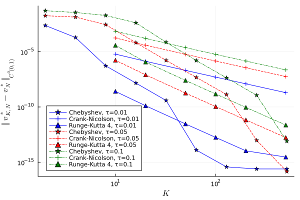
On Figure 2, we display the difference with the exact solution computed at $1000$ uniformly distributed points on the interval $[0,1]$ , and compare it with an order 2 Crank-Nicolson scheme as a function of $K$ . For the the Crank-Nicolson scheme, $K$ holds for the number of steps. As expected, the global in time Chebyshev approach exhibits spectral convergence, while the error evolves as $K^{-2}$ (convergence of order 2) for the Crank-Nicolson scheme. A Crank-Nicolson scheme with $K$ steps is cheaper than the procedure described above with $K$ functions, therefore, a higher value of $K$ does not necessarily mean that the computation is more expensive. The evolution of the computation time will be explored in the next example.

Refer to caption — Figure 1: $\left\|u^{*}_{K,L}-u^{*}\right\|_{\mathcal{C}^{0}\!\left({(-1,1)}\right)}$ for different choices of $L$ with $a=5$ and $\omega=20$

4.3 Periodic Schrödinger equation

We consider the Schrödinger equation on the two-dimensional torus $\mathbb{T}^{2}=(\mathbb{R}/\mathbb{Z})^{2}$ , and on the time interval $(-\tau,\tau)$ :

\begin{cases}i\partial_{t}u^{*}=(-\Delta_{x,y}+V(t))u^{*},\\ u^{*}(0)=u_{0},\end{cases}

(67)

where for all $t\in\mathbb{R}$ and $(x,y)\in\mathbb{T}^{2}$ , $V(t,x,y)=\cos((2\pi(x-c_{1}t))+\cos(2\pi(y-c_{2}t))+\cos(2\pi(x-y))$ .
A simple rescaling of the time variable shows that we can instead solve the following equation on $(-1,1)$

\begin{cases}i\partial_{t}u^{*}=\tau(-\Delta+V_{\tau}(t\tau))u^{*}\\ u^{*}(0)=u_{0}\end{cases}

(68)

where $V_{\tau}(t,x,y)=V(t\tau,x,y)$ .

The operator $-\Delta$ has a well-known diagonal structure with respect to the orthonormal system of Fourier modes $\operatorname{e}_{k,l}=\operatorname{e}^{2i\pi kx}\operatorname{e}^{2i\pi ly}$ , hence we will apply Theorem 3.1 and Corollary 3.1 with $H_{0}=-\Delta$ .

Define the discrete set

\Gamma_{N}=\operatorname{span}\{\operatorname{e}_{k,l}\}_{\begin{subarray}{c}-N/2\leq k<N/2\\ -N/2\leq l<N/2\end{subarray}}\subset L^{2}\!\left(\mathbb{T}^{2}\right),

(69)

and the orthogonal projector $\pi_{N}$ on $\Gamma_{N}$ . Since our goal here is to focus on the errors that arise from the time discretization, and not on the errors due to the truncation of the Fourier series, we will solve instead the "discrete" version of (67) that is well-posed in $\Gamma_{N}$ ,

\begin{cases}i\partial_{t}u^{*}_{N}=\tau(-\Delta+\pi_{N}V_{\tau}\pi_{N})u^{*}_{N},\\ u^{*}_{N}(0)=\pi_{N}u_{0}\in\Gamma_{N}.\end{cases}

(70)

Estimating the difference between the real solution $u^{*}$ to (67) and the solution $u^{*}_{N}$ to (70) is another problem that can be studied independently, but we do not consider it here.

We know from Corollary 3.1 that we can, instead of (70), solve the equivalent evolution equation

\begin{cases}i\partial_{t}v^{*}_{N}=\tau\operatorname{e}^{-it\tau\Delta}(\pi_{N}V_{\tau}\pi_{N})\operatorname{e}^{it\tau\Delta}v^{*}_{N},\\ v^{*}_{N}(0)=\pi_{N}u_{0}\in\Gamma_{N},\end{cases}

(71)

which is associated with the variational formulation

\min_{v\in H^{1}_{w}((-1,1),\Gamma_{N})}\left(\left|v(0)-\pi_{N}u_{0}\right|^{2}+\int_{-1}^{1}\,dt\,w(t)\left|i\partial_{t}v-\tau\operatorname{e}^{-it\tau\Delta}(\pi_{N}V_{\tau}\pi_{N})\operatorname{e}^{it\tau\Delta}v\right|^{2}\right).

(72)

We define the discrete subspace

\Sigma_{K,N}:=\left\{\sum_{k=0}^{K-1}v_{k}U_{k}(t)\,:\,(v_{k})_{k=0}^{K-1}\subset\Gamma_{N}\right\}\subset H^{1}_{w}((-1,1),L^{2}\!\left(\mathbb{T}^{2}\right)),

(73)

and the discrete solution $v^{*}_{K,N}$ as the unique solution to the restricted minimization problem

v^{*}_{K,N}=\operatorname*{argmin}_{v\in\Sigma_{K,N}}\left(\left|v(0)-\pi_{N}u_{0}\right|^{2}+\int_{-1}^{1}\,dt\,w(t)\left|i\partial_{t}v-\tau\operatorname{e}^{-it\tau\Delta}(\pi_{N}V_{\tau}\pi_{N})\operatorname{e}^{it\tau\Delta}v\right|^{2}\right).

(74)

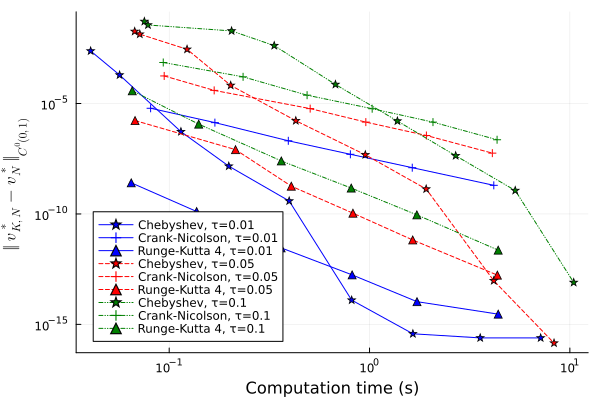
We employ a similar time discretization to that of Section 4.2, and the matrix associated with the quadratic form is built similarly, except that it involves block entries instead of scalar entries. The difference between the computed solution $v^{*}_{K,N}$ and $u^{*}_{N}$ is displayed in Figure 3 for several values of $\tau$ and $N=64$ . We compare it with an order 2 Crank-Nicolson scheme, and an order 4 Runge-Kutta scheme. As in the previous example, we observe a very fast convergence once $K$ reaches a certain threshold. Although the global space-time Chebyshev approach does not necessarily outperform classical time stepping scheme, it seems more efficient to reach very high precision when enough regularity is available, which is an expected behavior for a spectral method. On Figure 4, we display the computation time for several values of $K$ . We observe that the computational cost of the Chebyshev for a given value of $K$ has the same order of magnitude as the time-stepping schemes. The fact that it increases with $\tau$ is a consequence of the loss of quality of the preconditioner which leads to more iterations of the conjugate gradient algorithm used to solve the problem. Indeed, a smaller $\tau$ means that the equations is closer to the "free dynamics" that we use as a preconditioner. Finally, Figure 5 displays the errors of the different methods with respect to the computation cost. Since the computational cost of the different methods are very close, Figure 5 looks very much like Figure 2 with some corrections, and the same observations can be made.

5 Conclusion and perspectives

In this work, we establish a space-time variational formulation for the Schrödinger evolution equation (4). This formulation encompasses the case of many-body electronic Coulomb interaction with a bounded time-dependent potential and is in particular suitable for the design of a spectral in time discretization of the minimisation problem as illustrated in Section 4.

There are two main directions worth investigating. According to the tests performed in the 2D example, the variational formulation looks computationally more efficient for small time steps. Hence it seems natural to use the discretization with a spectral method within a time decomposition domain approach, like the parareal algorithm for instance where the spectral method could be used as a fine solver. The performance and the numerical analysis of the corresponding schemes would be worth investigating.

Another direction relies on the following proposition.

Proposition 5.1.

Let $\Sigma$ be any non empty weakly closed subset of $\mathcal{H}$ . Then the subset

H^{1}\!\left(I,\Sigma\right)=\left\{u\in H^{1}\!\left(I,\mathcal{H}\right)\,:\,u(t)\in\Sigma\text{ for any $t\in I$}\right\}.

is closed in $H^{1}\!\left(I,\mathcal{H}\right)$ for the weak topology.

Proof.

Since $H^{1}\!\left(I,\mathcal{H}\right)\hookrightarrow\mathcal{C}^{0}\!\left({I,\mathcal{H}}\right)$ , for any $t\in I$ the linear application

T_{t}:\left\{\begin{array}[]{rcl}H^{1}\!\left(I,\mathcal{H}\right)&\longrightarrow&\mathcal{H}\\ v&\longmapsto&v(t)\\ \end{array}\right.

is continuous.
Let $(v_{n})_{n\geq 0}\subset H^{1}\!\left(I,\Sigma\right)$ be a sequence which weakly converges to some $v$ in $H^{1}\!\left(I,\mathcal{H}\right)$ . Since any bounded linear operator between Banach spaces is also weakly continuous, this implies that for any $t\in I$ ,

v_{n}(t)=T_{t}v_{n}\mathop{\rightharpoonup}_{n\to+\infty}T_{t}v=v(t)\quad\text{in $\mathcal{H}$},

and the weak closedness of $\Sigma$ implies $v(t)\in\Sigma$ . ∎

One possible interesting choice for the set $\Sigma$ is some give set of functions which can be represented with low complexity, such as tensor formats, for instance the manifold of tensor trains with at most a given rank, or well-chosen neural network architectures. Proposition 5.1 implies that, for any value of the final time $T>0$ , there exists at least one minimizer to the minimization problem

u_{\Sigma}^{*}\in\operatorname*{argmin}_{v\in H^{1}\!\left(I,\Sigma\right)}F(v)

(75)

where $F$ is defined in (24).

As a consequence, for instance when $\Sigma$ is given as some low-rank tensor format, the variational principle studied here enables to obtain the existence of a dynamical low-rank approximation of $u^{*}$ whatever the value of the final time $T$ . This approximation is thus obtained through the variational principle (75) which is different from the classical Dirac-Frenkel one [4], for which, at least up to our knowledge, only local-in-time existence of solutions has been proved in the general case. The comparison of both types of dynamical low-rank approximations will be the object of a forthcoming article.

6 Proofs

The aim of this section is to gather the proofs of our main results.

6.1 Preliminary lemmas

Our analysis requires some tools from Kato’s smoothness theory. Throughout this section, $H_{0}$ is a self-adjoint operator on $\mathcal{H}$ with domain $D\!\left(H_{0}\right)$ , and $A$ is a symmetric closed operator on $\mathcal{H}$ .

Lemma 6.1.

Let $\varphi\in L^{1}(\mathbb{R},\mathcal{H})$ . Define for all $p\in\mathbb{R}$ ,

\widehat{\varphi}(p)=(2\pi)^{-\frac{1}{2}}\int_{\mathbb{R}}\,dt\,\operatorname{e}^{-ipt}\varphi(t).

(76)

Then

\int_{\mathbb{R}}\,dt\,\left|A\varphi(t)\right|^{2}=\int_{\mathbb{R}}\,dp\,\left|A\widehat{\varphi}(p)\right|^{2},

(77)

where the integrals are set equal to $\infty$ if we do not have that $\varphi(t)$ (resp. $\widehat{\varphi}(p)$ ) is in $D\!\left(A\right)$ for almost all $t\in\mathbb{R}$ .

Proof.

See [19], Chapter XIII, Section 3, Lemma 1, p142. ∎

Proposition 6.1.

The two following properties are equivalent

(i)

It holds that

c_{1}=\sup_{\varphi\in\mathcal{H},\;\left|\varphi\right|=1}\frac{1}{2}\int_{\mathbb{R}}\,dt\,\left|A\operatorname{e}^{-itH_{0}}\varphi\right|^{2}<\infty.

(ii)

It holds that $D\!\left(H_{0}\right)\subset D\!\left(A\right)$ , and

c_{2}=\sup_{\mu\in\mathbb{C}\setminus\mathbb{R},\;\varphi\in\mathcal{H},\,\left|\varphi\right|=1}\left|A(H_{0}-\mu)^{-1}\varphi\right|^{2}\left|\Im\mu\right|<\infty,

where $\Im\mu$ denotes the imaginary part of $\mu$ .

Moreover, when one of the conditions (i) or (ii) is satisfied, $c_{1}=c_{2}$ , and we say that $A$ is $H_{0}$ -smooth.

Proof.

See [19], Chapter XIII, Section 3, Theorem XIII.25, p146. ∎

From the proof of Proposition 6.1, we also extract the following lemma.

Lemma 6.2.

Let $H_{0}$ be a self-adjoint operator and $A$ a closed operator. For any $\varepsilon>0$ we have

\sup_{\varphi\in\mathcal{H},\;\left|\varphi\right|=1}\frac{1}{2}\int_{\mathbb{R}}\,dt\,\operatorname{e}^{-2\varepsilon\left|t\right|}\left|A\operatorname{e}^{-itH_{0}}\varphi\right|^{2}\leq\sup_{\lambda\in\mathbb{R},\;\varphi\in\mathcal{H},\,\left|\varphi\right|=1}\varepsilon\left|A(H_{0}-\lambda\pm i\varepsilon)^{-1}\varphi\right|^{2}.

Proof.

The following proof is just an extract of the proof of Proposition 6.1 (see [19], Chapter XIII, Section 3, Theorem XIII.25, p146.). Since it is instructive, we recall it here for the sake of completeness.
We first notice that, for a bounded operator $C$ on $\mathcal{H}$ , we have

\forall\psi_{1}\in D\!\left({A}^{*}\right),\;\forall\psi_{2}\in\mathcal{H},\quad\left({C}^{*}{A}^{*}\psi_{1}\middle|\psi_{2}\right)=\left({A}^{*}\psi_{1}\middle|C\psi_{2}\right),

from which we conclude that, the following statements are equivalent :

a)

$\operatorname{Ran}C\subset D\!\left(A\right)$ and $\left\|AC\right\|<\infty$

It holds

\sup_{\varphi\in D\!\left({A}^{*}\right),\left|\varphi\right|=1}\left|{C}^{*}{A}^{*}\varphi\right|<\infty.

Moreover, whenever a) and b) hold, we have the following equality:

\sup_{\varphi\in D\!\left({A}^{*}\right),\left|\varphi\right|=1}\left|{C}^{*}{A}^{*}\varphi\right|=\left\|AC\right\|.

Therefore, taking $C=(H_{0}-\lambda-i\varepsilon)^{-1}$ , we obtain

\begin{split}c_{\varepsilon}&:=\sup_{\lambda\in\mathbb{R},\;\varphi\in\mathcal{H},\,\,\left|\varphi\right|=1}\varepsilon\left|A(H_{0}-\lambda-i\varepsilon)^{-1}\varphi\right|^{2}\\ &=\sup_{\begin{subarray}{c}\lambda\in\mathbb{R}\\ \varphi\in D\!\left({A}^{*}\right),\,\left|\varphi\right|=1\end{subarray}}\varepsilon\left|(H_{0}-\lambda+i\varepsilon)^{-1}{A}^{*}\varphi\right|^{2}\\ &=\sup_{\begin{subarray}{c}\lambda\in\mathbb{R}\\ \varphi\in D\!\left({A}^{*}\right),\,\left|\varphi\right|=1\end{subarray}}\left(\varepsilon(H_{0}-\lambda-i\varepsilon)^{-1}(H_{0}-\lambda+i\varepsilon)^{-1}{A}^{*}\varphi\middle|{A}^{*}\varphi\right).\end{split}

The operator $\varepsilon(H_{0}-\lambda-i\varepsilon)^{-1}(H_{0}-\lambda+i\varepsilon)^{-1}=(2i)^{-1}((H_{0}-\lambda-i\varepsilon)^{-1}-(H_{0}-\lambda+i\varepsilon)^{-1})$ being bounded, self-adjoint and positive, we can consider its square root $K_{\varepsilon}(\lambda)$ , and the previous equality is equivalent to

\sup_{\begin{subarray}{c}\lambda\in\mathbb{R}\\ \varphi\in D\!\left({A}^{*}\right),\,\left|\varphi\right|=1\end{subarray}}\left|K_{\varepsilon}(\lambda){A}^{*}\varphi\right|^{2}\\ =\sup_{\lambda\in\mathbb{R},\,\varphi\in\mathcal{H},\,\left|\varphi\right|=1}\varepsilon\left|A(H_{0}-\lambda-i\varepsilon)^{-1}\varphi\right|^{2}=c_{\varepsilon}^{2},

hence, for any $\lambda\in\mathbb{R}$ $\operatorname{Ran}{K_{\varepsilon}(\lambda)}\subset D\!\left(A\right)$ and

\left\|AK_{\varepsilon}(\lambda)\right\|=c_{\varepsilon}

We now observe that

-i(H_{0}-\lambda-i\varepsilon)^{-1}=\int_{0}^{\infty}\,dt\,\operatorname{e}^{-\varepsilon t}\operatorname{e}^{i\lambda t}\operatorname{e}^{-itH_{0}}.

Using a similar identity for $(H_{0}-\lambda+i\varepsilon)^{-1}$ and applying Lemma 6.1 and the resolvent identity, we obtain, for all $\varphi\in\mathcal{H}$ ,

\begin{split}\int_{\mathbb{R}}\,dt\,\operatorname{e}^{-2\varepsilon\left|t\right|}\left|A\operatorname{e}^{-itH_{0}}\varphi\right|^{2}&=(2\pi)^{-1}\int_{\mathbb{R}}\,d\lambda\,\left|A((H_{0}-\lambda-i\varepsilon)^{-1}-(H_{0}-\lambda+i\varepsilon)^{-1})\varphi\right|^{2}\\ &=\frac{2}{\pi}\int_{\mathbb{R}}\,d\lambda\,\left|AK_{\varepsilon}(\lambda)^{2}\varphi\right|^{2}\\ &\leq\frac{2}{\pi}c_{\varepsilon}^{2}\int_{\mathbb{R}}\,d\lambda\,\left|K_{\varepsilon}(\lambda)\varphi\right|^{2}\\ &\leq\frac{2}{\pi}\frac{c_{\varepsilon}^{2}}{2i}\int_{\mathbb{R}}\,d\lambda\,\left(((H_{0}-\lambda-i\varepsilon)^{-1}-(H_{0}-\lambda+i\varepsilon)^{-1})\varphi\middle|\varphi\right).\end{split}

Denoting by $\,d\mu_{\varphi}\,$ the spectral measure of $\varphi$ for $H$ , we have

\begin{split}&\frac{2}{\pi}\frac{1}{2i}\int_{\mathbb{R}}\,d\lambda\,\left(((H_{0}-\lambda-i\varepsilon)^{-1}-(H_{0}-\lambda+i\varepsilon)^{-1})\varphi\middle|\varphi\right)\\ &=\frac{2}{\pi}\int_{\mathbb{R}}\,d\lambda\,\int_{\mathbb{R}}\,d\mu_{\varphi}\,(x)\frac{\varepsilon}{(x-\lambda)^{2}+\varepsilon^{2}}\\ &=\frac{2}{\pi}\int_{\mathbb{R}}\,d\mu_{\varphi}\,(x)\int_{\mathbb{R}}\,d\lambda\,\frac{\varepsilon}{(x-\lambda)^{2}+\varepsilon^{2}}\\ &=2\int_{\mathbb{R}}\,d\mu_{\varphi}\,(x)=2\left|\varphi\right|^{2},\end{split}

and the result follows. ∎

Using the previous results, we can prove

Proposition 6.2.

Assume that $H_{0}$ and $A$ satisfy the set of assumptions (A). Then, the operator $H=A+H_{0}$ is self-adjoint on $\mathcal{H}$ with domain $D\!\left(H\right)=D\!\left(H_{0}\right)$ , and there exists $C\geq 0$ such that

\forall T>0,\quad\forall\varphi\in\mathcal{H},\quad\int_{-T}^{T}\,dt\,\left|A\operatorname{e}^{-itH_{0}}\varphi\right|^{2}\leq C(1+T)\left|\varphi\right|^{2},

(78)

\forall T>0,\quad\forall\varphi\in\mathcal{H},\quad\int_{-T}^{T}\,dt\,\left|A\operatorname{e}^{-itH}\varphi\right|^{2}\leq C(1+T)\left|\varphi\right|^{2}.

(79)

Proof.

Let us introduce

c_{\varepsilon}:=\sup_{\lambda\in\mathbb{R}}\left\|A(H_{0}-\lambda\pm i\varepsilon)^{-1}\right\|<1,

(80)

for some $\varepsilon>0$ such that (A3) is satisfied.

First, let us prove that $H_{0}+A$ is self adjoint on $\mathcal{H}$ with domain $D\!\left(H_{0}\right)$ . Using (80), we obtain for all $\psi\in D\!\left(H_{0}\right)$ ,

\left|A\psi\right|=\left|A(H_{0}-i\varepsilon)^{-1}(H_{0}-i\varepsilon)\psi\right|\leq c_{\varepsilon}\left|(H_{0}-i\varepsilon)\psi\right|\leq c_{\varepsilon}\left|H_{0}\psi\right|+c_{\varepsilon}\varepsilon\left|\psi\right|.

This proves that $A$ is $H_{0}$ -bounded with relative bound lower than $1$ . Since we assumed $A$ symmetric, the self-adjointness of $H_{0}+A$ is a consequence of the Kato-Rellich theorem.

We now need to prove the estimates. We only prove the second one, since the proof for the first one is similar. For any $\lambda\in\mathbb{R}$ ,

(H-\lambda-i\varepsilon)^{-1}=\left((1+A(H_{0}-\lambda-i\varepsilon)^{-1})(H_{0}-\lambda-i\varepsilon)\right)^{-1}=(H_{0}-\lambda-i\varepsilon)^{-1}(1+A(H_{0}-\lambda-i\varepsilon)^{-1})^{-1},

hence it follows from Neumann’s inversion formula

\left|A(H-\lambda-i\varepsilon)^{-1}\right|=\left|A(H_{0}-\lambda-i\varepsilon)^{-1}(1+A(H_{0}-\lambda-i\varepsilon)^{-1})^{-1}\right|\leq\frac{c_{\varepsilon}}{1-c_{\varepsilon}}.

We can therefore apply Lemma 6.2, which shows that there exists a constant $C_{\varepsilon}\geq 0$ (which may vary along the calculations) such that

\forall\varphi\in\mathcal{H},\quad\int_{\mathbb{R}}\,dt\,\operatorname{e}^{-2\varepsilon\left|t\right|}\left|A\operatorname{e}^{-itH}\varphi\right|^{2}\leq C_{\varepsilon}\left|\varphi\right|^{2}.

Reducing the integration domain to $[0,\frac{1}{\varepsilon}]$ , we obtain

\forall\varphi\in\mathcal{H},\quad\int_{0}^{\frac{1}{\varepsilon}}\,dt\,\left|A\operatorname{e}^{-itH}\varphi\right|^{2}\leq C_{\varepsilon}\left|\varphi\right|^{2}.

Now, taking any integer $n\geq 1$ and $\varphi\in\mathcal{H}$ , we have

\begin{split}\int_{0}^{\frac{n}{\varepsilon}}\,dt\,\left|A\operatorname{e}^{-itH}\varphi\right|^{2}&=\sum_{k=0}^{n-1}\int_{\frac{k}{\varepsilon}}^{\frac{k+1}{\varepsilon}}\,dt\,\left|A\operatorname{e}^{-itH}\varphi\right|^{2}\\ &=\sum_{k=0}^{n-1}\int_{0}^{\frac{1}{\varepsilon}}\,dt\,\left|A\operatorname{e}^{-itH}(\operatorname{e}^{-i\frac{k}{\varepsilon}H}\varphi)\right|^{2}\\ &\leq C_{\varepsilon}\sum_{k=0}^{n-1}\left|\operatorname{e}^{-i\frac{k}{\varepsilon}H}\varphi\right|^{2}=C_{\varepsilon}n\left|\varphi\right|^{2}.\end{split}

Applying the same process for negative times, and writing any $T\geq 0$ as $T=\frac{n}{\varepsilon}+\tau$ , $0\leq\tau<\frac{1}{\varepsilon}$ , the estimate is proved. ∎

6.2 Proof of Theorem 3.1

We are now in position to prove Theorem 3.1.

Proof of Theorem 3.1.

Case (i): Assume that $H=H_{0}+A$ . Let $u\in\mathcal{X}_{H_{0}}$ . By Proposition 2.1, there exists $v\in H^{1}\!\left(I,\mathcal{H}\right)$ such that $u=\operatorname{e}^{-itH_{0}}v$ and $\left\|(i\partial_{t}-H_{0})u\right\|_{L^{2}\!\left(I,\mathcal{H}\right)}=\left\|\partial_{t}v\right\|_{L^{2}\!\left(I,\mathcal{H}\right)}$ . Therefore,

\begin{split}\left\|Au\right\|_{L^{2}\!\left(I,\mathcal{H}\right)}&=\left\|A\operatorname{e}^{-itH_{0}}\left(u(0)+\int_{0}^{t}\,ds\,\partial_{t}v(s)\right)\right\|_{L^{2}\!\left(I,\mathcal{H}\right)}\\ &\leq\left\|A\operatorname{e}^{-itH_{0}}v(0)\right\|_{L^{2}\!\left(I,\mathcal{H}\right)}+\int_{0}^{T}\,ds\,\left\|\mathbf{1}_{s\leq t}A\operatorname{e}^{-itH_{0}}\partial_{t}v(s)\right\|_{L^{2}\!\left(I,\mathcal{H}\right)}.\end{split}

Proposition 6.2 shows the existence of a constant $C>0$ such that

\begin{split}\left\|Au\right\|_{L^{2}\!\left(I,\mathcal{H}\right)}&\leq C\sqrt{1+T}\left|v(0)\right|+C\sqrt{1+T}\int_{0}^{T}\,ds\,\left|\partial_{t}v(s)\right|\\ &\leq C\sqrt{1+T}\left|v(0)\right|+C\sqrt{1+T}\sqrt{T}\left\|\partial_{t}v\right\|_{L^{2}\!\left(I,\mathcal{H}\right)}\\ &\leq C\sqrt{1+T}\left(\left|u(0)\right|^{2}+T\left\|(i\partial_{t}-H_{0})u\right\|_{L^{2}\!\left(I,\mathcal{H}\right)}^{2}\right)^{\frac{1}{2}}\\ &\leq C\sqrt{1+T}\left\|u\right\|_{\mathcal{X}_{H_{0}}}.\end{split}

(81)

Thus, $(i\partial_{t}-H)u=(i\partial_{t}-H_{0})u-Au\in L^{2}\!\left(I,\mathcal{H}\right)$ , that is, $u\in\mathcal{X}_{H}$ and

\begin{split}\left\|u\right\|_{\mathcal{X}_{H}}&\leq\left|u(0)\right|+\sqrt{T}\left\|(i\partial_{t}-H_{0}-A)u\right\|_{L^{2}\!\left(I,\mathcal{H}\right)}\\ &\leq\left|u(0)\right|+\sqrt{T}\left\|(i\partial_{t}-H_{0})u\right\|_{L^{2}\!\left(I,\mathcal{H}\right)}+\sqrt{T}\left\|Au\right\|_{L^{2}\!\left(I,\mathcal{H}\right)}\\ &\leq C(\left\|u\right\|_{\mathcal{X}_{H_{0}}}+\sqrt{T}\sqrt{1+T}\left\|u\right\|_{\mathcal{X}_{H_{0}}})\\ &\leq C(1+T)\left\|u\right\|_{\mathcal{X}_{H_{0}}}.\end{split}

(82)

This proves the right inequality in (21).

We now turn to the left inequality in (21). Let $u\in\mathcal{X}_{H}$ . Applying Proposition 6.2, we obtain the existence of a $C>0$ such that

\forall\varphi\in\mathcal{H},\quad\left\|A\operatorname{e}^{-itH}\varphi\right\|_{L^{2}\!\left(I,\mathcal{H}\right)}\leq C\sqrt{1+T}\left|\varphi\right|.

The rest of the proof can be carried without change, simply by permuting $H_{0}$ and $H$ .

Case (ii): We now turn to the case $H(t)=H_{0}+A+B(t)$ .

Let $u\in\mathcal{X}_{H_{0}}$ , then

\begin{split}N(u)^{2}&=\left|u(0)\right|^{2}+T\left\|(i\partial_{t}-H_{0}-A-B(t))u(t)\right\|_{L^{2}\!\left(I,\mathcal{H}\right)}^{2}\\ &\leq\left|u(0)\right|^{2}+2T\left\|(i\partial_{t}-H_{0}-A)u(t)\right\|_{L^{2}\!\left(I,\mathcal{H}\right)}^{2}+2TM^{2}\left\|u\right\|_{L^{2}\!\left(I,\mathcal{H}\right)}^{2}.\end{split}

The sum of the two first terms can be estimated by the first part of Theorem 3.1 as follows,

\left|u(0)\right|^{2}+2T\left\|(i\partial_{t}-H_{0}-A)u(t)\right\|_{L^{2}\!\left(I,\mathcal{H}\right)}^{2}\leq C(1+T)^{2}\left\|u\right\|_{\mathcal{X}_{H_{0}}}^{2}

and for the third term we write

\left\|u\right\|_{L^{2}\!\left(I,\mathcal{H}\right)}\leq\sqrt{T}\left\|u\right\|_{\mathcal{C}^{0}\!\left({I,\mathcal{H}}\right)}\leq\sqrt{2T}\left\|u\right\|_{\mathcal{X}_{H_{0}}}.

Therefore,

N(u)^{2}\leq C(1+T)^{2}\left\|u\right\|_{\mathcal{X}_{H_{0}}}^{2},

which is the right-hand estimate of (23).

Conversely, let $u\in\mathcal{X}_{H_{0}}$ and write $u_{0}=u(0)$ and $f(t)=(i\partial_{t}-H_{0}-A-B(t))u(t)$ . Then it follows from the continuity estimate in Proposition A.2 that

\left\|u\right\|_{L^{2}\!\left(I,\mathcal{H}\right)}^{2}\leq T\left\|u\right\|_{\mathcal{C}^{0}\!\left({I,\mathcal{H}}\right)}^{2}\leq 2T(\left|u(0)\right|^{2}+T\left\|f\right\|_{L^{2}\!\left(I,\mathcal{H}\right)}^{2}),

therefore,

\begin{split}\left\|u\right\|_{\mathcal{X}_{H}}^{2}&\leq 2(N(u)^{2}+M^{2}T\left\|u\right\|_{L^{2}\!\left(I,\mathcal{H}\right)}^{2})\\ &\leq C(\left\|u\right\|_{\mathcal{X}_{H}(t)}^{2}+T^{2}\left\|u\right\|_{\mathcal{X}_{H}(t)}^{2}).\end{split}

Using the first part of the proof, we finally obtain

\left\|u\right\|_{\mathcal{X}_{H_{0}}}\leq C(1+T)\left\|u\right\|_{\mathcal{X}_{H}}\leq C(1+T)^{2}N(u),

which concludes the proof. ∎

6.3 Proof of Theorem 3.2

Proof of Theorem 3.2.

To prove Theorem 3.2, notice that if $A$ is $H_{0}$ -smooth, then (81) in the proof above can be replaced by

\left\|Au\right\|_{L^{2}\!\left(I,\mathcal{H}\right)}\leq C\left\|u\right\|_{\mathcal{X}_{H_{0}}}.

The result is proved by adapting (82). ∎

6.4 Proof of Corollary 3.1

Proof of Corollary 3.1.

Let $v=\operatorname{e}^{itH_{0}}u\in H^{1}\!\left(I,\mathcal{H}\right)$ , then

\begin{split}(i\partial_{t}-\operatorname{e}^{itH_{0}}A\operatorname{e}^{-itH_{0}})v-\operatorname{e}^{itH_{0}}f&=i\partial_{t}\operatorname{e}^{itH_{0}}u-\operatorname{e}^{itH_{0}}Au-\operatorname{e}^{itH_{0}}f\\ &=\operatorname{e}^{itH_{0}}(i\partial_{t}-H_{0})u-\operatorname{e}^{itH_{0}}Au-\operatorname{e}^{itH_{0}}(i\partial_{t}-H)u^{*}\\ &=\operatorname{e}^{itH_{0}}(i\partial_{t}-H)(u-u^{*}).\end{split}

It immediately follows that

F(v)=\left\|u-u^{*}\right\|_{\mathcal{X}_{H}}^{2},

and the result is a consequence of (21) and the fact that $\left\|u-u^{*}\right\|_{\mathcal{X}_{H_{0}}}=\left\|v-v^{*}\right\|_{H^{1}\!\left(I,\mathcal{H}\right)}$ . ∎

6.5 Proof of Proposition 3.1

The proof of this result in the case $N=1$ and $V(x)=\frac{1}{\left|x\right|}$ , is non trivial, and can be found in [15] or [3] :

Proposition 6.3.

For any $\varphi\in L^{2}\!\left(\mathbb{R}^{3}\right)$ , let $\psi(t,x)=\frac{1}{|x|}(\operatorname{e}^{it\Delta}\varphi)(t,x)$ for $t\in\mathbb{R}$ and $x\in\mathbb{R}^{3}$ . Then,

\left\|\psi\right\|_{L^{2}\!\left(\mathbb{R}_{t}\times\mathbb{R}^{3}_{x}\right)}\leq 2\sqrt{\frac{2}{\pi}}\left\|\varphi\right\|_{L^{2}\!\left(\mathbb{R}^{3}\right)}.

(83)

We deduce Proposition 3.1 from Proposition 6.3 as follows.

Proof of Proposition 3.1.

We only need to prove the result in the case $V=\frac{1}{\left|x_{1}\right|}$ . All the other cases can be reduced to this one through a unitary change of variables : For $\frac{1}{\left|x_{\ell}-X_{k}\right|}$ we set $y_{j}=x_{j}$ for $j\neq l$ and $y_{\ell}=x_{\ell}-X_{k}$ . For $\frac{1}{x_{k}-x_{\ell}}$ we set $y_{j}=x_{j}$ for $j\not\in\left\{k,l\right\}$ , $y_{k}=\frac{x_{k}-x_{\ell}}{\sqrt{2}}$ and $y_{\ell}=\frac{x_{k}+x_{\ell}}{\sqrt{2}}$ (which explains why a $\frac{1}{\sqrt{2}}$ appears with these terms).

Let $\varphi\in L^{2}\!\left(\mathbb{R}^{3N}\right)$ . Using the fact that $L^{2}\!\left(\mathbb{R}^{3N}\right)=L^{2}\!\left(\mathbb{R}^{3}\right)\otimes L^{2}\!\left(\mathbb{R}^{3(N-1)}\right)$ , introducing the singular value decomposition of $\varphi$ , there exist two orthogonal sequences $(v_{k})_{k\geq 1}\subset L^{2}\!\left(\mathbb{R}^{3}\right)$ , $(w_{k})_{k\geq 1}\subset L^{2}\!\left(\mathbb{R}^{3(N-1)}\right)$ such that for almost all $x_{1}\in\mathbb{R}^{3}$ and $X=(x_{2},...,x_{N})\in\mathbb{R}^{3(N-1)}$

\varphi(x_{1},X)=\sum_{k\geq 1}v_{k}(x_{1})w_{k}(X),

the sum above being possibly infinite. Therefore,

\begin{split}\left\|\frac{\operatorname{e}^{it\Delta}\varphi}{\left|x_{1}\right|}\right\|_{L^{2}\!\left(\mathbb{R}\times\mathbb{R}^{3N}\right)}^{2}&=\left\|\sum_{k\geq 1}\left(\frac{\operatorname{e}^{it\Delta_{x_{1}}}v_{k}}{\left|x_{1}\right|}\right)\otimes\left(\operatorname{e}^{it\Delta_{X}}w_{k}\right)\right\|_{L^{2}\!\left(\mathbb{R}\times\mathbb{R}^{3N}\right)}^{2}\\ &=\sum_{k\geq 1}\left\|\left(\frac{\operatorname{e}^{it\Delta_{x_{1}}}v_{k}}{\left|x_{1}\right|}\right)\otimes\left(\operatorname{e}^{it\Delta_{X}}w_{k}\right)\right\|_{L^{2}\!\left(\mathbb{R}\times\mathbb{R}^{3N}\right)}^{2},\end{split}

where we used the fact that, for each $t$ , $(\operatorname{e}^{it\Delta_{X}}w_{k})_{k}$ is an orthogonal family of $L^{2}\!\left(\mathbb{R}^{3N}\right)$ . Thus,

\begin{split}\left\|\frac{\operatorname{e}^{it\Delta}\varphi}{\left|x_{1}\right|}\right\|_{L^{2}\!\left(\mathbb{R}\times\mathbb{R}^{3N}\right)}^{2}&=\sum_{k\geq 1}\int_{\mathbb{R}}\,dt\,\left\|\frac{\operatorname{e}^{it\Delta_{x_{1}}}v_{k}}{\left|x_{1}\right|}\right\|_{L^{2}\!\left(\mathbb{R}^{3}\right)}^{2}\left\|\operatorname{e}^{it\Delta_{X}}w_{k}\right\|_{L^{2}\!\left(\mathbb{R}^{3(N-1)}\right)}^{2}\\ &\leq\sum_{k\geq 1}\left(2\sqrt{\frac{2}{\pi}}\right)^{2}\left\|v_{k}\right\|_{L^{2}\!\left(\mathbb{R}^{3}\right)}^{2}\left\|w_{k}\right\|_{L^{2}\!\left(\mathbb{R}^{3(N-1)}\right)}^{2}\\ &=\left(2\sqrt{\frac{2}{\pi}}\right)^{2}\left\|\varphi\right\|_{L^{2}\!\left(\mathbb{R}^{3N}\right)}^{2}.\end{split}

∎

Appendix A Weak solutions to the Schrödinger equation

Let $J\subset\mathbb{R}$ be a bounded interval such that $0\in\overline{J}$ and $T=\sup_{t\in J}\left|t\right|$ . We define weak solutions to the evolution equation (4) as follows:

Definition A.1.

Let $u,f\in L^{2}\!\left(J,\mathcal{H}\right)$ . We say that $(i\partial_{t}-H-B(t))u=f$ holds weakly if and only if

\forall\varphi\in\mathcal{C}_{c}^{0}\!\left({J,D\!\left(H\right)}\right)\cap\mathcal{C}_{c}^{1}\!\left({J,\mathcal{H}}\right),\quad\left(u\middle|(i\partial_{t}-H)\varphi\right)_{L^{2}\!\left(J,\mathcal{H}\right)}=\left(f\middle|\varphi\right)_{L^{2}\!\left(J,\mathcal{H}\right)},

(84)

where $D\!\left(H\right)$ is equipped with the graph norm of $H$ .

We first deal with the case $B(t)=0$ .

Proposition A.1.

Let $u\in L^{2}\!\left(J,\mathcal{H}\right)$ , and $v=\operatorname{e}^{itH}u$ . The following are equivalent :

1.

$(i\partial_{t}-H)u\in L^{2}\!\left(J,\mathcal{H}\right)$ .
2.

$i\partial_{t}v\in L^{2}\!\left(J,\mathcal{H}\right)$ .

In particular, if 1. and 2. hold, $u$ and $v$ both belong to $\mathcal{C}^{0}\!\left({J,\mathcal{H}}\right)$ . Moreover, in this case, $i\partial_{t}v=\operatorname{e}^{itH}(i\partial_{t}-H)u$ , and

\forall t\in J,\quad u(t)=\operatorname{e}^{-itH}u(0)-i\int_{0}^{t}\,ds\,\operatorname{e}^{-i(t-s)H}(i\partial_{t}-H)u(s).

(85)

Proof.

Assume $(i\partial_{t}-H)u=f\in L^{2}\!\left(J,\mathcal{H}\right)$ , then, for any $\varphi\in\mathcal{C}_{c}^{\infty}\!\left({J,D\!\left(H^{2}\right)}\right)$ ,

\left(v\middle|i\partial_{t}\varphi\right)_{L^{2}\!\left(J,\mathcal{H}\right)}=\left(u\middle|\operatorname{e}^{-itH}i\partial_{t}\varphi\right)_{L^{2}\!\left(J,\mathcal{H}\right)}=\left(u\middle|(i\partial_{t}-H)\operatorname{e}^{-itH}i\partial_{t}\varphi\right)_{L^{2}\!\left(J,\mathcal{H}\right)}=\left(f\middle|\operatorname{e}^{-itH}\varphi\right)_{L^{2}\!\left(J,\mathcal{H}\right)}.

By density, this identity extends to all $\varphi\in\mathcal{C}_{c}^{1}\!\left({J,\mathcal{H}}\right)$ , and we conclude that $v\in H^{1}\!\left(J,\mathcal{H}\right)$ with $i\partial_{t}v=\operatorname{e}^{itH}f$ .

Conversely, assume $i\partial_{t}v=g\in L^{2}\!\left(J,\mathcal{H}\right)$ . Then for any $\varphi\in\mathcal{C}_{c}^{\infty}\!\left({J,D\!\left(H^{2}\right)}\right)$ ,

\left(u\middle|(i\partial_{t}-H)\varphi\right)_{L^{2}\!\left(J,\mathcal{H}\right)}=\left(v\middle|\operatorname{e}^{itH}(i\partial_{t}-H)\varphi\right)_{L^{2}\!\left(J,\mathcal{H}\right)}=\left(v\middle|i\partial_{t}\operatorname{e}^{itH}\varphi\right)_{L^{2}\!\left(J,\mathcal{H}\right)}=\left(g\middle|\operatorname{e}^{itH}\varphi\right)_{L^{2}\!\left(J,\mathcal{H}\right)}.

By density, the identity extends to all $\varphi\in\mathcal{C}_{c}^{0}\!\left({J,D\!\left(H\right)}\right)\cap\mathcal{C}_{c}^{1}\!\left({J,\mathcal{H}}\right)$ , so $(i\partial_{t}-H)u=\operatorname{e}^{-itH}g\in L^{2}\!\left(J,\mathcal{H}\right)$ . Moreover, we then have for all $t\in J$

\begin{split}u(t)&=\operatorname{e}^{-itH}v(t)=\operatorname{e}^{-itH}(v(0)-i\int_{0}^{t}\,ds\,g(s))\\ &=\operatorname{e}^{-itH}u(0)-i\int_{0}^{t}\,ds\,\operatorname{e}^{-i(t-s)H}(i\partial_{t}-H)u(s).\end{split}

∎

Corollary A.1.

For any $f\in L^{2}\!\left(J,\mathcal{H}\right)$ and $u_{0}\in\mathcal{H}$ , there exists exactly one $u^{*}\in L^{2}\!\left(J,\mathcal{H}\right)$ such that $(i\partial_{t}-H)u^{*}=f$ and $u^{*}(0)=u_{0}$ .

Proof.

Existence: Let $f\in L^{2}\!\left(J,\mathcal{H}\right)$ . Define

v^{*}(t)=u_{0}-i\int_{0}^{t}\,ds\,\operatorname{e}^{isH}f(s),

and $u^{*}=\operatorname{e}^{-itH}v^{*}$ . Then, by Proposition A.1, $(\partial_{t}-H)u^{*}=\operatorname{e}^{-itH}\operatorname{e}^{itH}i\partial_{t}v^{*}=f$ , and $u^{*}(0)=u_{0}$ .

Uniqueness: Assume $(i\partial_{t}-H)u^{*}_{1}=(i\partial_{t}-H)u^{*}_{2}=f\in L^{2}\!\left(J,\mathcal{H}\right)$ and $u^{*}_{1}(0)=u^{*}_{2}(0)=u_{0}$ . Define $v^{*}_{j}=\operatorname{e}^{itH}u^{*}_{j}$ ( $j=1,2$ ), we then have $\partial_{t}v^{*}_{1}=\partial_{t}v^{*}_{2}$ . Since $v^{*}_{1}(0)=v^{*}_{2}(0)=u_{0}$ , uniqueness follows. ∎

We now add a time-dependent part $B(t)$ , assumed to be a strongly continuous family of uniformly bounded self-adjoint operators (that is, for any $t\in J$ , $B(t)$ is a bounded self-adjoint operator, and $\sup_{t\in J}\left\|B(t)\right\|<\infty$ ).

Proposition A.2.

For any $f\in L^{2}\!\left(J,\mathcal{H}\right)$ and $u_{0}\in\mathcal{H}$ there exist a unique $u^{*}\in L^{2}\!\left(J,\mathcal{H}\right)$ such that $(i\partial_{t}-H-B(t))u^{*}=f$ and $u(0)=u_{0}$ . Furthermore, the following continuity estimate holds:

\left\|u^{*}\right\|_{\mathcal{C}^{0}\!\left({J,\mathcal{H}}\right)}\leq\sqrt{2}\left(\left|u_{0}\right|^{2}+T\left\|f\right\|_{L^{2}\!\left(J,\mathcal{H}\right)}^{2}\right)^{\frac{1}{2}}

(86)

Proof.

The result is proved by a standard fixed-point argument for ODEs. For simplicity, we assume here $J=(0,T)$ for some $T>0$ . Set

M=\sup_{t\in J}\left\|B(s)\right\|.

We also define, for $\mu>0$ ,

\forall u\in L^{2}\!\left(J,\mathcal{H}\right),\quad\left\|u\right\|_{L^{2}\!\left(J,\mathcal{H}\right)}^{\prime}=\left(\int_{0}^{T}\,dt\,\operatorname{e}^{-\mu t}\left|u(t)\right|^{2}\right)^{\frac{1}{2}},

which is a norm on $L^{2}\!\left(J,\mathcal{H}\right)$ equivalent to $\left\|\cdot\right\|_{L^{2}\!\left(J,\mathcal{H}\right)}$ .

For any $u\in L^{2}\!\left(J,\mathcal{H}\right)$ and $t\in J$ , set

\Phi(u)(t)=\operatorname{e}^{-itH}u_{0}-i\int_{0}^{t}\,ds\,\operatorname{e}^{-i(t-s)H}(f(s)-B(s)u(s)).

Clearly $\Phi(u)\in L^{2}\!\left(J,\mathcal{H}\right)$ , and for any $u,v\in L^{2}\!\left(J,\mathcal{H}\right)$ ,

\begin{split}{\left\|\Phi(u)-\Phi(v)\right\|_{L^{2}\!\left(J,\mathcal{H}\right)}^{\prime}}^{2}&=\int_{0}^{T}\,dt\,\operatorname{e}^{-\mu t}\left|\int_{0}^{t}\,ds\,\operatorname{e}^{-i(t-s)H}B(s)(v(s)-u(s))\right|^{2}\\ &\leq M^{2}T\int_{0}^{T}\,dt\,\operatorname{e}^{-\mu t}\int_{0}^{T}\,ds\,\left|u(s)-v(s)\right|^{2}\\ &\leq M^{2}T\int_{0}^{T}\,ds\,\left|u(s)-v(s)\right|^{2}\int_{s}^{\infty}\,dt\,\operatorname{e}^{-\mu t}\\ &\leq\frac{M^{2}T}{\mu}\int_{0}^{T}\,ds\,\operatorname{e}^{-\mu s}\left|u(s)-v(s)\right|^{2}.\end{split}

Choosing $\mu$ such that $\frac{M^{2}T}{\mu}<1$ , this proves that $\Phi$ is contractive for $\left\|\cdot\right\|_{L^{2}\!\left(J,\mathcal{H}\right)}^{\prime}$ , hence admits a unique fixed point $u^{*}$ which satisfies for all $t\in\mathcal{H}$

u^{*}(t)=\operatorname{e}^{-itH}u_{0}-i\int_{0}^{t}\,ds\,\operatorname{e}^{-i(t-s)H}(f(s)-B(s)u^{*}(s)),

(87)

which, by Proposition A.1, is equivalent to $(i\partial_{t}-H-B(t))u=f$ and $u(0)=u_{0}$ .

To prove the continuity estimate, we first assume $f\in\mathcal{C}^{0}\!\left({J,\mathcal{H}}\right)$ , and write for any $t\in J$

\left|u^{*}(t)\right|^{2}=\left|u_{0}-i\int_{0}^{t}\,ds\,\operatorname{e}^{isH}(f(s)-B(s)u^{*}(s))\right|^{2},

from which we deduce

\begin{split}\frac{\,d\,}{\,dt\,}\left|u^{*}(t)\right|^{2}&=2\Re\langle u_{0}-i\int_{0}^{t}\,ds\,\operatorname{e}^{isH}(f(s)-B(s)u^{*}(s)),-i\operatorname{e}^{itH}(f(t)-B(t)u^{*}(t))\rangle\\ &=2\Im\langle u^{*}(t),f(t)-B(t)u^{*}(t)\rangle=2\Im\langle u^{*}(t),f(t)\rangle.\end{split}

This yields

\forall t\in J,\quad\left|\frac{\,d\,}{\,dt\,}\left|u^{*}(t)\right|^{2}\right|\leq 2\left|u^{*}(t)\right|\left|f(t)\right|.

Let $\varepsilon>0$ and $w_{\varepsilon}(t)=\varepsilon+\left|u_{0}\right|+\int_{0}^{t}\,ds\,\left|f(s)\right|$ . Let $K_{\varepsilon}=\left\{w_{\varepsilon}\geq\left|u^{*}\right|\right\}\subset\overline{J}$ , which is closed (by continuity of $w$ and $u^{*}$ ) and contains $0$ . Now assume $t_{0}:=\inf\overline{J}\setminus K_{\varepsilon}<T$ . By continuity, it holds $\left|u^{*}(t_{0})\right|=w(t_{0})\geq\varepsilon>0$ , and there exists a $\delta>0$ such that $[t_{0},t_{0}+\delta]\subset J$ and $\left|u^{*}(t)\right|$ for every $t\in[t_{0},t_{0}+\delta]$ . Therefore,

\forall t\in[t_{0}-\delta,t_{0}+\delta],\quad 2\left|u^{*}(t)\right|\frac{\,d\,}{\,dt\,}\left|u^{*}(t)\right|=\frac{\,d\,}{\,dt\,}\left|u^{*}(t)\right|^{2}\leq 2\left|f(t)\right|\left|u^{*}(t)\right|,

which yields

\forall t\in[t_{0},t_{0}+\delta],\quad\frac{\,d\,}{\,dt\,}\left|u^{*}(t)\right|\leq\left|f(t)\right|.

It follows by integration that

\forall t\in[t_{0},t_{0}+\delta],\quad\left|u^{*}(t)\right|\leq\left|u^{*}(t_{0})\right|+\int_{t_{0}}^{t}\,ds\,\left|f(s)\right|=w(t),

which contradicts the definition of $t_{0}$ . Therefore,

\forall t\in\overline{J},\quad\left|u^{*}(t)\right|\leq w_{\varepsilon}(t)\leq\varepsilon+\left|u_{0}\right|+\sqrt{T}\left\|f\right\|_{L^{2}\!\left(J,\mathcal{H}\right)}\leq\varepsilon+\sqrt{2}\left(\left|u_{0}\right|^{2}+T\left\|f\right\|_{L^{2}\!\left(J,\mathcal{H}\right)}^{2}\right)^{\frac{1}{2}}.

Since this holds for any $\varepsilon>0$ , we obtain the desired inequality.

For general $f\in L^{2}\!\left(J,\mathcal{H}\right)$ , we take a sequence $(f_{n})_{n\geq 0}$ such that $\left\|f_{n}-f\right\|_{L^{2}\!\left(J,\mathcal{H}\right)}\to 0$ , and define $u^{*}_{n}$ the unique element of $L^{2}\!\left(J,\mathcal{H}\right)$ such that

u^{*}_{n}(t)=\operatorname{e}^{-itH}u_{0}-i\int_{0}^{t}\,ds\,\operatorname{e}^{-i(t-s)H}(f_{n}(s)-B(s)u^{*}_{n}(s)).

(88)

As earlier, we compare $u^{*}_{n}$ and $u^{*}$ in term of $\left\|\cdot\right\|^{\prime}_{L^{2}\!\left(J,\mathcal{H}\right)}$ , and obtain with (87) and (88)

{\left\|u_{n}^{*}-u^{*}\right\|^{\prime}_{L^{2}\!\left(J,\mathcal{H}\right)}}^{2}\leq C\left\|f_{n}-f\right\|_{L^{2}\!\left(J,\mathcal{H}\right)}^{2}+\frac{M^{2}T}{\mu}{\left\|u_{n}^{*}-u^{*}\right\|^{\prime}_{L^{2}\!\left(J,\mathcal{H}\right)}}^{2},

yielding

\left\|u_{n}^{*}-u^{*}\right\|^{\prime}_{L^{2}\!\left(J,\mathcal{H}\right)}\leq C\left\|f_{n}-f\right\|_{L^{2}\!\left(J,\mathcal{H}\right)},

for some constant $C>0$ . This proves that $u^{*}_{n}\to u^{*}$ in $L^{2}\!\left(J,\mathcal{H}\right)$ , and using (87) and (88) again we deduce that $u^{*}_{n}\to u^{*}$ in $\mathcal{C}^{0}\!\left({J,\mathcal{H}}\right)$ . The result appears by taking $n\to\infty$ in

\forall n\geq 0,\quad\left\|u^{*}_{n}\right\|_{\mathcal{C}^{0}\!\left({J,\mathcal{H}}\right)}\leq\sqrt{2}\left(\left|u_{0}\right|^{2}+T\left\|f_{n}\right\|_{L^{2}\!\left(J,\mathcal{H}\right)}^{2}\right)^{\frac{1}{2}}.

∎

Appendix B Ackowledgements

This publication is part of a project that has received funding from the European Research Council (ERC) under the European Union’s Horizon 2020 Research and Innovation Programme – Grant Agreement n^∘ 101077204. We are also very thankful to Caroline Lasser, Christian Lubich and Elena Celedoni for enlightening discussions on this work.

References

[1] Markus Bachmayr. Low-rank tensor methods for partial differential equations. Acta Numerica, 32:1–121, 2023.
[2] Markus Bachmayr, Reinhold Schneider, and André Uschmajew. Tensor networks and hierarchical tensors for the solution of high-dimensional partial differential equations. Foundations of Computational Mathematics, 16:1423–1472, 2016.
[3] Nicolas Burq, Fabrice Planchon, John G. Stalker, and A. Shadi Tahvildar-Zadeh. Strichartz Estimates for the Wave and Schrödinger Equations with Potentials of Critical Decay. Indiana University Mathematics Journal, 53(6):1665–1680, 2004.
[4] Dajana Conte and Christian Lubich. An error analysis of the multi-configuration time-dependent Hartree method of quantum dynamics. ESAIM: Mathematical Modelling and Numerical Analysis, 44(4):759–780, July 2010.
[5] Leszek Demkowicz, Jayadeep Gopalakrishnan, Sriram Nagaraj, and Paulina Sepulveda. A spacetime DPG method for the Schrödinger equation. SIAM Journal on Numerical Analysis, 55(4):1740–1759, 2017.
[6] Alexandre Ern and Jean-Luc Guermond. Linear stabilization for first-order PDEs. In Handbook of Numerical Analysis, volume 17, pages 265–288. Elsevier, 2016.
[7] Antonio Falcó, Wolfgang Hackbusch, and Anthony Nouy. On the Dirac-Frenkel variational principle on tensor Banach spaces. Foundations of computational mathematics, 19:159–204, 2019.
[8] Sergio Gómez and Andrea Moiola. A Space-Time Trefftz Discontinuous Galerkin Method for the Linear Schrödinger Equation. SIAM Journal on Numerical Analysis, 60(2):688–714, 2022.
[9] Sergio Gómez and Andrea Moiola. A space–time DG method for the Schrödinger equation with variable potential. Advances in Computational Mathematics, 50(2):15, 2024.
[10] Clément Guillot, Virginie Ehrlacher, and Mi-Song Dupuy. Repository for "A space-time variational formulation for the many-body electronic Schrödinger evolution equation". https://doi.org/10.5281/zenodo.11353969, May 2024.
[11] Stefan Hain and Karsten Urban. An Ultra-Weak Space-Time Variational Formulation for the Schrödinger Equation. 2022.
[12] Tuomas Hytönen, Jan Van Neerven, Mark Veraar, and Lutz Weis. Analysis in Banach spaces, volume 12. Springer, 2016.
[13] Ohannes Karakashian and Charalambos Makridakis. A space-time finite element method for the nonlinear Schrödinger equation: the discontinuous Galerkin method. Mathematics of computation, 67(222):479–499, 1998.
[14] Ohannes Karakashian and Charalambos Makridakis. A space-time finite element method for the nonlinear Schrödinger equation: the continuous Galerkin method. SIAM journal on numerical analysis, 36(6):1779–1807, 1999.
[15] Tosio Kato and Kenji Yajima. Some examples of smooth operators and the associated smoothing effect. Rev. Math. Phys., 1(4):481–496, 1989.
[16] Örs Legeza, Thorsten Rohwedder, Reinhold Schneider, and Szilárd Szalay. Tensor product approximation (DMRG) and coupled cluster method in quantum chemistry. Many-Electron Approaches in Physics, Chemistry and Mathematics: A Multidisciplinary View, pages 53–76, 2014.
[17] Christian Lubich. A variational splitting integrator for quantum molecular dynamics. Applied numerical mathematics, 48(3-4):355–368, 2004.
[18] Christian Lubich. On variational approximations in quantum molecular dynamics. Mathematics of computation, 74(250):765–779, 2005.
[19] Michael Reed and Barry Simon. Methods of modern mathematical physics. IV. Analysis of operators. New York San Francisco London : Academic Press , cop. 1978, New York San Francisco London, 1978.

A space-time variational formulation for the many-body electronic Schrödinger evolution equation

Abstract

1 Introduction

2 Preliminaries

2.1 Notations and weak solutions

Definition 2.1.

Remark 2.1.

2.2 Duhamel formula and functional space

Proposition 2.1.

Proposition 2.2.

Proof.

3 Space-time variational formulation for the Schrödinger equation

3.1 Global space-time formulation in H1​(I,ℋ)superscript𝐻1𝐼ℋH^{1}(I,\mathcal{H})

Lemma 3.1.

Proof.

Remark 3.1.

Theorem 3.1.

Corollary 3.1.

Remark 3.2.

Theorem 3.2.

3.2 Application to electronic many-body Schrödinger operators

Proposition 3.1.

Remark 3.3.

Corollary 3.2.

Theorem 3.3.

3.3 Dual formulation

Proposition 3.2.

Lemma 3.2.

Proof.

Proposition 3.3.

Proof.

Corollary 3.3.

Proof of Corollary 3.3.

4 Numerical implementation with spectral methods

4.1 Time regularity of the solution

Theorem 4.1.

Proof of Theorem 4.1.

4.2 A first basic example

4.3 Periodic Schrödinger equation

5 Conclusion and perspectives

Proposition 5.1.

Proof.

6 Proofs

6.1 Preliminary lemmas

Lemma 6.1.

Proof.

Proposition 6.1.

Proof.

Lemma 6.2.

Proof.

Proposition 6.2.

Proof.

6.2 Proof of Theorem 3.1

Proof of Theorem 3.1.

6.3 Proof of Theorem 3.2

Proof of Theorem 3.2.

6.4 Proof of Corollary 3.1

Proof of Corollary 3.1.

6.5 Proof of Proposition 3.1

Proposition 6.3.

Proof of Proposition 3.1.

Appendix A Weak solutions to the Schrödinger equation

Definition A.1.

Proposition A.1.

Proof.

Corollary A.1.

Proof.

Proposition A.2.

Proof.

Appendix B Ackowledgements

References

3.1 Global space-time formulation in $H^{1}(I,\mathcal{H})$