Triple Component Matrix Factorization: Untangling Global, Local, and Noisy Components

TCMF Naichen Shi \emailnaichens@umich.edu
\addrDepartment of Industrial & Operations Engineering
University of Michigan
Ann Arbor, MI 48109, USA \ANDTCMF Salar Fattahi \emailfattahi@umich.edu
\addrDepartment of Industrial & Operations Engineering
University of Michigan
Ann Arbor, MI 48109, USA \ANDTCMF Raed Al Kontar \emailalkontar@umich.edu
\addrDepartment of Industrial & Operations Engineering
University of Michigan
Ann Arbor, MI 48109, USA Corresponding author

Abstract

In this work, we study the problem of common and unique feature extraction from noisy data. When we have $N$ observation matrices from $N$ different and associated sources corrupted by sparse and potentially gross noise, can we recover the common and unique components from these noisy observations? This is a challenging task as the number of parameters to estimate is approximately thrice the number of observations. Despite the difficulty, we propose an intuitive alternating minimization algorithm called triple component matrix factorization (TCMF) to recover the three components exactly. TCMF is distinguished from existing works in literature thanks to two salient features. First, TCMF is a principled method to separate the three components given noisy observations provably. Second, the bulk of the computation in TCMF can be distributed. On the technical side, we formulate the problem as a constrained nonconvex nonsmooth optimization problem. Despite the intricate nature of the problem, we provide a Taylor series characterization of its solution by solving the corresponding Karush–Kuhn–Tucker conditions. Using this characterization, we can show that the alternating minimization algorithm makes significant progress at each iteration and converges into the ground truth at a linear rate. Numerical experiments in video segmentation and anomaly detection highlight the superior feature extraction abilities of TCMF.

Keywords: Matrix Factorization, Heterogeneity, Alternating minimization, Sparse noise, Outlier identification

1 Introduction

In the era of Big Data, an important task is to find low-rank features from high-dimensional observations. Methods including principal component analysis (Hotelling, 1933), low-rank matrix factorization (Koren et al., 2009), and dictionary learning (Aharon et al., 2006), have found success in numerous fields of statistics and machine learning (Wright and Ma, 2022). Among them, matrix factorization (MF) is an efficient method to identify the features that best explain the observation matrices.

Despite the wide popularity, standard MF methods are known to be brittle in the presence of outliers with huge noise (Candès et al., 2011). These noises are often sparse but can have large norms. A series of methods (e.g., (Candès et al., 2011; Netrapalli et al., 2014; Wong and Lee, 2017; Fattahi and Sojoudi, 2020; Chen et al., 2021)) have been developed to estimate low-rank features from data that contain outliers. When the portion of outliers is not too large, one can provably identify the outliers and the low-rank components with convex programming (Candès et al., 2011) or nonconvex optimization algorithms equipped with convergence guarantees (Netrapalli et al., 2014).

Recently, there has been a growing number of applications where data are acquired from diverse but connected sources, such as smartphones, car sensors, or medical records from different patients. This type of data displays both mutual and individual characteristics. For instance, in biostatistics, the measurements of different miRNA and gene expressions from the same set of samples can reveal co-varying patterns yet exhibit heterogeneous trends (Lock et al., 2013). Statistical modeling of the common information among all data sources and the specific information for each source is of central interest in these applications. Multiple works propose to recover such common and unique features by minimizing the square norm of the residuals of fitting (Lock et al., 2013; Zhou et al., 2015; Gaynanova and Li, 2019; Park and Lock, 2020; Lee and Choi, 2009; Yang and Michailidis, 2016; Shi and Kontar, 2024; Shi et al., 2023; Liang et al., 2023). These methods prove to be useful in aligning genetics features (Lock et al., 2013), visualizing bone and soft tissues in X-ray images (Zhou et al., 2015), functional magnetic resonance imaging (Kashyap et al., 2019), surveillance video segmentation (Shi and Kontar, 2024), stocks market analysis (Shi et al., 2023), and many more.

Though these algorithms achieve decent performance on multiple applications, they rely on least square estimates, which are not robust to outliers in data. Real-world data are commonly corrupted by outliers (Tan et al., 2005). Factors including measurement errors or sensor malfunctions can give rise to large noise in data. These outliers can substantially skew the estimation of low-rank features. As such, we attempt to answer the following question.

rgb]0.95,0.95,0.95 Question: How can one provably identify low-rank common and unique information robustly from data corrupted by outlier noise?

A natural thought is to borrow techniques in robust PCA to handle outlier noise. Indeed, there exist a few heuristic methods in literature (Sagonas et al., 2017; Panagakis et al., 2015; Ponzi et al., 2021) to find robust estimates of shared and unique features. These methods often use $\ell_{1}$ regularization (Sagonas et al., 2017; Panagakis et al., 2015) or Huber loss (Ponzi et al., 2021) to accommodate the sparsity of noise. However, these algorithms are mainly based on heuristics and lack theoretical guarantees, thus potentially compromising the quality of their outputs. A theoretically justifiable method to identify low-rank shared and unique components from outlier noise is still lacking. In this paper, we will study the question rigorously and develop an efficient algorithm to solve it.

2 Problem Statement

We consider the framework where $N$ observation matrices $\mathbf{M}_{(1)},\mathbf{M}_{(2)},\cdots,\mathbf{M}_{(N)}$ come from $N\in\mathbb{N}^{+}$ different but associated sources. These matrices $\mathbf{M}_{(i)}\in\mathbb{R}^{n_{1}\times n_{2,(i)}}$ have the same number of features $n_{1}$ . To model their commonality and uniqueness, we assume each matrix is driven by $r_{1}$ shared factors and $r_{2,(i)}$ unique factors and contaminated by potentially gross noise. More specifically, we consider the model where the observation $\mathbf{M}_{(i)}$ from source $i$ is generated by,

\mathbf{M}_{(i)}={\mathbf{U}^{\star}}_{g}{\mathbf{V}^{\star}}_{(i),g}^{T}+{\mathbf{U}^{\star}}_{(i),l}{\mathbf{V}^{\star}}_{(i),l}^{T}+{\mathbf{S}^{\star}}_{(i)}

(1)

, where ${\mathbf{U}^{\star}}_{g}\in\mathbb{R}^{n_{1}\times r_{1}}$ , ${\mathbf{V}^{\star}}_{(i),g}\in\mathbb{R}^{n_{2,(i)}\times r_{1}}$ , ${\mathbf{U}^{\star}}_{(i),l}\in\mathbb{R}^{n_{1}\times r_{2,(i)}}$ , ${\mathbf{V}^{\star}}_{(i),l}\in\mathbb{R}^{n_{2,(i)}\times r_{2,(i)}}$ , ${\mathbf{S}^{\star}}_{(i)}\in\mathbb{R}^{n_{1}\times n_{2,(i)}}$ . We use ^⋆ to denote the ground truth. $r_{1}$ is the rank of global (shared) feature matrices, and $r_{2,(i)}$ is the rank of local (unique) feature matrix from source $i$ . The matrix ${\mathbf{U}^{\star}}_{g}{\mathbf{V}^{\star}}_{(i),g}^{T}$ models the shared low-rank part of the observation matrix, as the column space is the same across different sources. ${\mathbf{U}^{\star}}_{(i),l}{\mathbf{V}^{\star}}_{(i),l}^{T}$ models the unique low-rank part. ${\mathbf{S}^{\star}}_{(i)}$ models the noise from source $i$ .

In matrix factorization problems, the representations ${\mathbf{U}^{\star}}$ and ${\mathbf{V}^{\star}}$ often correspond to latent data features. For instance, in recommender systems, ${\mathbf{U}^{\star}}$ can be interpreted as user features that reveal their preferences on different items in the latent space (Koren et al., 2009). For better interpretability, it is often desirable to have the underlying features disentangled so that each feature can vary independently of others (Higgins et al., 2017). Under this rationale, we consider the model where shared and unique factors are orthogonal,

{\mathbf{U}^{\star}}_{g}^{T}{\mathbf{U}^{\star}}_{(i),l}=0,\ \forall i\in[N],

(2)

, , where $[N]$ denotes the set $\{1,2,\cdots,N\}$ . The orthogonality of features implies that the shared and unique features span different subspaces, thus describing different patterns in the observation. The orthogonal condition (2) is thus an inductive bias that reflects our prior belief about the independence between common and unique factors and naturally models a diverse range of applications, such as miRNA and gene expression (Lock et al., 2013), human faces (Zhou et al., 2015), and many more (Sagonas et al., 2017; Shi and Kontar, 2024).

The noise term ${\mathbf{S}^{\star}}_{(i)}$ in (1) models the sparse and large noise, where only a small fraction of ${\mathbf{S}^{\star}}_{(i)}$ registers as nonzero. The noise sparsity is extensively invoked in literature, particularly when datasets are plagued by outliers (Candès et al., 2011; Netrapalli et al., 2014; Chen et al., 2020, 2021).

2.1 Challenges

Given data generation model (1), our task is to separate common, individual, and noise components. The task seems Herculean as the problem is under-definite: we need to estimate three sets of parameters from one set of observations. There are two major challenges associated with the problem,

Challenge 1: New identifiability conditions are needed. Standard analysis in robust PCA (Candès et al., 2011; Netrapalli et al., 2014) often uses the incoherence condition to distinguish low-rank components from sparse noise. However, the incoherence condition alone is insufficient to guarantee the separability between common and unique features. Since there are infinitely many ways in which shared, unique, and noise components can form the observation matrices, it is not apparent whether untangling them is even feasible. Thus, the crux of our investigation is to understand when the separation is possible.

Fortunately, we show that a group of conditions–known here as identifiability conditions–exists that can ensure the precise retrieval of the shared, unique, and sparse noise. Intuitively, these identifiability conditions require the three components to have “little overlaps”.

Based on these conditions, we will develop an alternating minimization algorithm called TCMF to iteratively update the three components. An illustration of the algorithm is shown in the left graph in Figure 1. The hard-thresholding step finds the closest sparse matrix for the data noise. We use JIMF to denote a subroutine that represents a group of algorithms (e.g., (Lock et al., 2013; Shi and Kontar, 2024)) to identify common and unique low-rank features. In essence, JIMF solves a sub-problem in TCMF. It is worth noting that there exist multiple algorithms in literature to implement JIMF, many of which can produce high-quality outputs. With the implemented JIMF, TCMF applies hard thresholding and JIMF alternatively to estimate the sparse, as well as common and unique low-rank components. The left graph of Figure 1 offers an intuitive understanding of how estimates of various components progress toward the ground truth with each iterative step.

Refer to caption — Figure 1: Left: An illustration of TCMF’s update trajectory. The purple and blue curves represent the spaces for the low-rank and sparse matrices. The algorithm alternatively performs hard thresholding and JIMF, making the updates closer and closer to the ground truth. Middle: An illustration showing why insufficient understanding about the output of JIMF can be problematic in the convergence analysis. Right: Our contribution to represent the solution into a Taylor-like series.

Challenge 2: New analysis tools are needed. Showing the exact recovery of low-rank and sparse components is not easy. Even in standard robust PCA, one needs to apply highly nontrivial analytical techniques to provide theoretical guarantees. For example, Robust PCA (Candès et al., 2011) relies on a “golfing scheme” to construct dual variables that ensure the uniqueness of a convex optimization problem. Nonconvex robust PCA (Netrapalli et al., 2014) applies a perturbation analysis of SVD to quantify the improvement of the algorithm per iteration. These techniques are tailored for standard robust PCA and cannot be directly extended to the case where both common and unique features are involved, which increases the complexity of the analysis. The major difficulty stems from the fact that TCMF updates the low-rank common and unique components by another iterative algorithm JIMF. Unlike robust PCA, the output of JIMF does not have a closed-form formula. This conceptual hurdle is illustrated in the middle graph of Figure 1. As a result, novel analysis tools are needed to justify the convergence of the proposed TCMF.

One of our key contributions in tackling the challenge is to develop innovative analysis tools by solving the Karush–Kuhn–Tucker conditions of the objective of JIMF and express the solutions into a Taylor-like series. From the Taylor-like series, we can precisely characterize the output of JIMF, thereby showing the series converge to a close estimate of the ground truth shared and unique features.

The Taylor-like series is depicted in the right graph of Figure 1. Perhaps surprisingly, regardless of the choice of the subroutine JIMF, as long as JIMF finds a close estimate of the optimal solutions to a subproblem, its output can be represented by an infinite series. The series describes the optimal solution of the subproblem and is independent of the intermediate steps in JIMF. The derivation and analysis of Taylor-like series have stand-alone values in the theoretical research of the sensitivity analysis of matrix factorization. With the new analysis tool, we are able to show that even if the JIMF only outputs a reasonable approximate solution, the meta-algorithm TCMF can still take advantage of the information in such an inexact solution to refine the estimates of the three components. We will elaborate on the Taylor-like series in greater detail in Section 6 and the Appendix.

We summarize our contributions in the following.

2.2 Summary of Contributions

Identifiability conditions. We discover a group of identifiability conditions sufficient for the almost exact recovery of common, unique, and sparse components from noisy observation matrices. Essentially, the identifiability conditions require that the fraction of nonzero entries in the noise not be too large, the factor matrices be incoherent, and unique factors be misaligned. The first two conditions are needed even in the standard analysis of the robust PCA, while the third condition is essential for the disentanglement of the shared and unique components.

Efficient and distributed algorithm. We propose a constrained nonconvex nonsmooth matrix factorization problem to solve the shared, unique, and sparse components. Despite the nonconvexity of the problem, we design a meta-algorithm called Triple Component Matrix Factorization (TCMF) to solve the problem. Our approach is able to leverage a wide range of existing methods for separating the common and unique components to precision $\epsilon$ . Furthermore, JIMF can be distributed if the subroutine JIMF is distributed.

Convergence guarantee. We show that, under the identifiability conditions, our proposed TCMF has a convergence guarantee. To the best of our knowledge, such a guarantee is the first of its kind, as it ensures the recovery of common, unique, and noise components to high precision. Our theoretical analysis introduces new techniques to solve the KKT conditions in Taylor-like series and bound each term in the series. It sheds light on the sensitivity analysis with the $\ell_{\infty}$ norm.

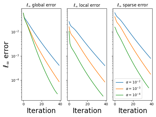
Case studies. We use a wide range of numerical experiments to demonstrate the application of TCMF in different case studies, as well as the effectiveness of our proposed method. Numerical experiments corroborate theoretical convergence results. Also, the case studies on video segmentation and anomaly detection showcase the benefits of untangling shared, unique, and noisy components.

In the rest of the paper, we provide a comprehensive review of the literature in Section 3. Then, we elaborate on the conditions sufficient for the separation of the three components in Section 4. In Section 5, we introduce the alternating minimization algorithm. We present our convergence theorem in Section 6 and discuss the key insights in the proof and how they solve challenge 2. In Section 7, we demonstrate the numerical experiment results. The detailed proofs are relegated to the Appendix for brevity of the main paper.

3 Related Work

Matrix Factorization There are numerous works that analyze the theoretical and practical properties of first-order algorithms that solve the (asymmetric) matrix factorization problem $\min_{\mathbf{U},\mathbf{V}}\left\lVert{\mathbf{M}-\mathbf{U}\mathbf{V}^{T}}\right\rVert_{F}^{2}$ or its variants (Li et al., 2018; Ye and Du, 2021; Sun and Luo, 2016; Park et al., 2017; Tu et al., 2016). Among them, Sun and Luo (2016) analyzes the local landscape of the optimization problem and establishes the local linear convergence of a series of first-order algorithms. Park et al. (2017); Ge et al. (2017) study the global geometry of the optimization problem. Tu et al. (2016) proposes the Rectangular Procrustes Flow algorithm that is proved to converge linearly into the ground truth under proper initialization and a balancing regularization. Recently, Ye and Du (2021) shows that gradient descent with small and random initialization can converge to the ground truth.

Robust PCA When the observation is corrupted by sparse and potentially large noise, several approaches can still identify the low-rank components. An exemplary work is Robust PCA (Candès et al., 2011), which proposes an elegant convex optimization problem called principal component pursuit that uses nuclear norm and $\ell_{1}$ norm to promote the sparsity and low-rankness of the solutions. It is proved that under incoherence assumptions, the solution of the convex optimization is unique and corresponds to the ground truth. Several works also consider the problem of matrix completion under outlier noise (Wong and Lee, 2017; Chen et al., 2021). Nonconvex robust PCA (Netrapalli et al., 2014) improves the computational efficiency of principal component pursuit by proposing a nonconvex formulation and using an alternating projection algorithm to solve it. Though the formulation is nonconvex, the alternating projection algorithm is also proved to recover the ground truth exactly under incoherence and sparsity requirements. For the special case of rank-1 robust PCA, Fattahi and Sojoudi (2020) show that a simple sub-gradient method applies directly to the nonsmooth $\ell_{1}$ -loss provably recovers the low-rank component and sparse noise, under the same incoherence and sparsity requirements. To model a broader set of noise, Meng and De La Torre (2013) consider a mixture of Gaussian noise models and exploit the EM algorithm to estimate the low-rank components. Robust PCA has found successful applications in video segmentation (Bouwmans and Zahzah, 2014), image processing (Vaswani et al., 2018), change point detection (Xiao et al., 2020), and many more. Nevertheless, the formulations of robust PCA focus on shared low-rank features among all data and neglect unique components.

Distributed matrix factorization The emergence of edge computation has prompted the research on distributed matrix factorization. Gemulla et al. (2011) exploits distributed gradient descent to factorize large matrices. Chai et al. (2021) proposes a cryptographic framework where multiple clients use their local data to collaboratively factorize a matrix without leaking private information to the server. These works use one set of feature matrices $\mathbf{U}$ and $\mathbf{V}$ to fit data from all clients, thus also neglecting the feature differences from different sources as well as the possible outliers in data. Our method TCMF is distributed when its subroutine JIMF is distributed. Different from conventional distributed matrix factorization, TCMF can find common and unique components simultaneously while remaining robust in the presence of outliers.

Joint and individual feature extraction The literature on using MF to identify shared and unique features abound (Lock et al., 2013; Zhou et al., 2015; Gaynanova and Li, 2019; Park and Lock, 2020; Lee and Choi, 2009; Yang and Michailidis, 2016; Shi and Kontar, 2024; Liang et al., 2023; Shi et al., 2023). Among them, JIVE (Lock et al., 2013), COBE (Zhou et al., 2015), PerPCA (Shi and Kontar, 2024), and HMF (Shi et al., 2023) uses mutually orthogonal features to model the shared and unique components. SLIDE (Gaynanova and Li, 2019) and BIDIFAC (Park and Lock, 2020) do not pose orthogonality constraints but use regularizations to encourage the unique features to have small norms. GNMF (Lee and Choi, 2009) and iNMF (Yang and Michailidis, 2016) further add nonnegativity constraints to the factor matrices. In particular, PerPCA (Shi and Kontar, 2024) and HMF (Shi et al., 2023) are two distributed algorithms that are guaranteed to converge to the optimal solutions under proper conditions. It is worth mentioning that these methods do not account for sparse noise in the observations. In this work, we remedy this challenge by utilizing existing methods as basic building blocks for our approach, which focuses on simultaneously separating shared and unique features as well as noise components.

Robust shared and unique feature extraction As discussed, a few heuristic methods also attempt to find the shared and unique features when data are corrupted by large noise (Sagonas et al., 2017; Ponzi et al., 2021; Panagakis et al., 2015). Amid them, RaJIVE (Ponzi et al., 2021) employs robust SVD (Zhang et al., 2013) to remove noise from the observations and then uses a variant of JIVE (Feng et al., 2018) to separate common and unique components. RJIVE (Sagonas et al., 2017) proposes a constrained optimization formulation to minimize the $\ell_{1}$ norm of the fitting residuals and exploits ADMM to solve the problem. RCICA (Panagakis et al., 2015) adopts a similar optimization objective but uses a regularization to encourage the similarity of common subspaces and only works for $N=2$ cases. Though these methods can achieve decent performance in applications including facial expression synthesis and audio-visual fusion, they are based on heuristics and it is not clear whether their output converges to the ground truth common and unique factors. In contrast, we prove that TCMF is guaranteed to recover the ground truths and use a few numerical examples to show that TCMF indeed recover more meaningful components.

4 Identifiability Conditions

Our goal is to decouple the common components, unique components, and the sparse noise, given a group of data observations $\left\{\mathbf{M}_{(i)}\right\}_{i=1}^{N}$ . At first glance, such decoupling may seem impossible or even ill-defined: roughly speaking, the number of unknown variables, namely global components, local components, and noise, are thrice the number of observed data matrices $\left\{\mathbf{M}_{(i)}\right\}_{i=1}^{N}$ , and hence, there are infinite number of decouplings that can give rise to the same $\mathbf{M}_{(i)}$ .

The very first question to ask is whether such decoupling is possible and, if so, which properties can ensure the identifiability of three components. Intriguingly, we are able to prove that the exact decoupling of shared features, unique features, and noise is possible if there is “little overlap” among the three components. Below, we will formalize this intuition in more detail. Though intuitive, it turns out that these conditions can guarantee the identifiability of the shared components, unique components, and the sparse noise.

4.1 Sparsity

As discussed, identifying arbitrarily dense and large noise from signals is not possible. Hence, we consider sparse noise where only a small fraction of observations are corrupted. To characterize the sparsity of ${\mathbf{S}^{\star}}_{(i)}$ , we use the following definition of $\alpha$ -sparsity.

Definition 1

( $\alpha$ -sparsity) A matrix $\mathbf{S}\in\mathbb{R}^{n_{1}\times n_{2}}$ is $\alpha$ -sparse if at most $\alpha n_{1}$ entries in each column and at most $\alpha n_{2}$ entries in each row are nonzero.

The definition follows from that of Netrapalli et al. (2014). In Definition 1, $\alpha$ characterizes the maximum portion of corrupted entries in each row and each column. Intuitively, if a matrix is $\alpha$ -sparse with small $\alpha$ , then its nonzero entries are “spread out” instead of concentrated on specific columns or rows.

4.2 Incoherence

It is shown that distinguishing sparse components from arbitrary low-rank components is also hard (Candès et al., 2011; Netrapalli et al., 2014). As a simple counterexample, the matrix $\mathbf{M}=\mathbf{e}_{i}\mathbf{e}_{j}^{T}$ , where we use $\mathbf{e}_{i}$ to denote the basis vector of axis $i$ , has its $ij$ -th entry to be $1$ and all other entries to be $0$ . This matrix has rank $1$ , and is also sparse since it has only one nonzero entry. Thus, deciding whether it is sparse or low rank is difficult as it satisfies both requirements.

From the above analysis, one can see that the low-rank components should not be sparse. In other words, to be distinguishable from the sparse noise, their elements should be sufficiently spread out. In the literature, this requirement is often characterized by the so-called incoherence condition (Candès et al., 2011; Netrapalli et al., 2014).

Definition 2

( $\mu$ -incoherence) A matrix $\mathbf{U}\in\mathbb{R}^{n\times r}$ is $\mu$ -incoherent if

\max_{i}\left\lVert\mathbf{e}_{i}^{T}\mathbf{U}\right\rVert_{2}\leq\frac{\mu\sqrt{r}}{\sqrt{n}}

, where $\mathbf{e}_{i}\in\mathbb{R}^{n}$ is the standard basis vector of axis $i$ , defined as $\mathbf{e}_{i}=(0,0,...0,1,0,...0)^{T}$

The incoherence condition restricts the maximum row-wise $\ell_{2}$ norm of a matrix $\mathbf{U}$ , thus preventing the entries of $\mathbf{U}$ from being too concentrated on a few specific axes.

Remember that in model (1), ${\mathbf{U}^{\star}}_{g}{\mathbf{V}^{\star}}_{(i),g}^{T}$ and ${\mathbf{U}^{\star}}_{(i),l}{\mathbf{V}^{\star}}_{(i),l}^{T}$ represent the global (shared) and local (unique) factors. For any $n\geq r$ , we use $\mathbb{O}^{n\times r}$ to denote the set of $n$ by $r$ matrices whose column vectors are orthonormal, $\mathbb{O}^{n\times r}=\{\mathbf{W}\in\mathbb{R}^{n\times r}|\mathbf{W}^{T}\mathbf{W}=\mathbf{I}\}$ . We assume the SVD of ${\mathbf{U}^{\star}}_{g}{\mathbf{V}^{\star}}_{(i),g}^{T}$ and ${\mathbf{U}^{\star}}_{(i),l}{\mathbf{V}^{\star}}_{(i),l}^{T}$ has the following form,

\left\{\begin{aligned} &{\mathbf{U}^{\star}}_{g}{\mathbf{V}^{\star}}_{(i),g}^{T}={\mathbf{H}^{\star}}_{g}{\mathbf{\Sigma}^{\star}}_{(i),g}{\mathbf{W}^{\star}}_{(i),g}^{T}\\ &{\mathbf{U}^{\star}}_{(i),l}{\mathbf{V}^{\star}}_{(i),l}^{T}={\mathbf{H}^{\star}}_{(i),l}{\mathbf{\Sigma}^{\star}}_{(i),l}{\mathbf{W}^{\star}}_{(i),l}^{T}\end{aligned}\right.

(3)

, where ${\mathbf{H}^{\star}}_{g}\in\mathbb{O}^{n_{1}\times r_{1}}$ , ${\mathbf{W}^{\star}}_{(i),g}\in\mathbb{O}^{n_{2}\times r_{1}}$ , ${\mathbf{H}^{\star}}_{(i),l}\in\mathbb{O}^{n_{1}\times r_{2}}$ . Moreover, ${\mathbf{W}^{\star}}_{(i),l}\in\mathbb{O}^{n_{2}\times r_{2}}$ are orthogonal matrices, ${\mathbf{\Sigma}^{\star}}_{(i),g}\in\mathbb{R}^{r_{1}\times r_{1}}$ and ${\mathbf{\Sigma}^{\star}}_{(i),l}\in\mathbb{R}^{r_{2}\times r_{2}}$ are positive diagonal matrices. In (3), we consider the case where the global and local column and row singular vectors are orthogonal, i.e., ${\mathbf{H}^{\star}}_{g}^{T}{\mathbf{H}^{\star}}_{(i),l}=0$ and ${\mathbf{W}^{\star}}_{(i),g}^{T}{\mathbf{W}^{\star}}_{(i),l}=0$ .

To avoid overlapping between sparse and low-rank components, we assume the row and column singular vectors ${\mathbf{H}^{\star}}_{g}$ , ${\mathbf{H}^{\star}}_{(i),l}$ , ${\mathbf{W}^{\star}}_{(i),g}$ , and ${\mathbf{W}^{\star}}_{(i),l}$ are all $\mu$ -incoherent. This assumption ensures that the low-rank components do not have entries too concentrated on specific rows or columns. As a result, the incoherence on singular vectors encourages the low-rank components to distribute evenly on all entries, which is distinguished from sparse noises that are nonzero on a small fraction of entries.

4.3 Misalignment

As discussed in (3), we use orthogonality between shared and unique features ${\hat{\mathbf{H}}}^{\star}{}_{g}^{T}{\hat{\mathbf{H}}}^{\star}{}_{(i),l}=0$ to encode our prior belief about the independence of different features. This is equivalent to ${\mathbf{U}^{\star}}_{g}^{T}{\mathbf{U}^{\star}}_{(i),l}=0$ . Such orthogonality, however, is still insufficient to guarantee the identifiability of shared and unique factors.

To see this, consider a counterexample where all ${\mathbf{U}^{\star}}_{(i),l}$ ’s are equal, i.e., ${\mathbf{U}^{\star}}_{(1),l}={\mathbf{U}^{\star}}_{(2),l}=\cdots={\mathbf{U}^{\star}}_{(N),l}$ . In this case, “unique” factors are also shared among all observation matrices. Thus, separating them from the ground truth ${\mathbf{U}^{\star}}_{g}$ is not possible. From this counterexample, we can see that it is essential for the local features not to be perfectly aligned with each other. Next, we formally introduce the notion of misalignment. For a full column-rank matrix $\mathbf{U}\in\mathbb{R}^{d\times n}$ , we define the projection matrix $\mathbf{P}_{\mathbf{U}}\in\mathbb{R}^{d\times d}$ as $\mathbf{P}_{\mathbf{U}}=\mathbf{U}\left(\mathbf{U}^{T}\mathbf{U}\right)^{-1}\mathbf{U}^{T}$ .

Definition 3

( $\theta$ -misalignment) We say $\{{\mathbf{U}^{\star}}_{(i),l}\}$ are $\theta$ -misaligned if there exists a positive constant $\theta\in(0,1)$ such that:

\lambda_{\max}\left(\frac{1}{N}\sum_{i=1}^{N}\mathbf{P}_{{\mathbf{U}^{\star}}_{(i),l}}\right)\leq 1-\theta

(4)

By the triangular inequality of $\lambda_{\max}\left(\cdot\right)$ , we know $\lambda_{\max}\left(\frac{1}{N}\sum_{i=1}^{N}\mathbf{P}_{{\mathbf{U}^{\star}}_{(i),l}}\right)\leq\frac{1}{N}\sum_{i=1}^{N}\lambda_{\max}\left(\mathbf{P}_{{\mathbf{U}^{\star}}_{(i),l}}\right)=1$ . Thus, the introduced $\theta$ is always nonnegative. Indeed, all $\mathbf{P}_{{\mathbf{U}^{\star}}_{(i),l}}$ ’s have a common nonempty eigenspace with eigenvalue $1$ if and only if $\theta=0$ . Thus, the $\theta$ -misalignment condition requires that the subspaces spanned by all unique factors do not contain a common subspace. On the contrary, all global features are shared; hence, the subspaces spanned by these features are also identical. This comparison shows that the misalignment condition unequivocally distinguishes unique features from shared ones.

As a concrete example, consider $N=2$ and $\mathbf{U}_{(1),l}=\left(\cos\vartheta,\sin\vartheta\right)^{T}$ , $\mathbf{U}_{(2),l}=\left(\cos\vartheta,-\sin\vartheta\right)^{T}$ for $\vartheta\in[0,\frac{\pi}{4}]$ . Indeed, the angle between $\mathbf{U}_{(1),l}$ and $\mathbf{U}_{(2),l}$ is $2\vartheta$ and

\frac{1}{2}\left(\mathbf{P}_{\mathbf{U}_{(1),l}}+\mathbf{P}_{\mathbf{U}_{(2),l}}\right)=\left(\begin{aligned} \cos^{2}\vartheta,&\quad 0\\ 0,&\quad\sin^{2}\vartheta\\ \end{aligned}\right)

Hence, by definition, $\theta=\sin^{2}\vartheta$ . We can thus clearly see that when $\vartheta$ increases, the $\mathbf{U}_{(1),l}$ and $\mathbf{U}_{(2),l}$ become more misaligned.

The notion of $\theta$ -misalignment is first proposed by Shi and Kontar (2024) and intimately related to the uniqueness conditions in Lock et al. (2013).

5 Algorithm

The introduced identifiability conditions restrict the overlaps between shared, unique, and sparse components. It remains to develop algorithms to untangle the three parts from $N$ matrices. In Section 5.1, we introduce a constrained optimization formulation, and in Section 5.2, we propose an alternating minimization program to decouple the three parts. The alternating minimization requires solving subproblems to distinguish shared features from unique ones.

Throughout the paper, we use $\left\lVert\mathbf{A}\right\rVert$ or $\left\lVert\mathbf{A}\right\rVert_{2}$ to denote the operator norm of a matrix $\mathbf{A}\in\mathbb{R}^{m\times n}$ and $\left\lVert\mathbf{A}\right\rVert_{F}$ to denote the Frobenius norm of $\mathbf{A}$ . We use $r$ to denote $r=r_{1}+r_{2}$ .

5.1 Constrained Nonconvex Nonsmooth Optimization

We design a constrained optimization problem to decouple the three components. The decision variables $\mathbf{x}$ include features, coefficients, and sparse noise estimates: $\mathbf{x}=\left(\mathbf{U}_{g},\{\mathbf{U}_{(i),l},\mathbf{V}_{(i),g},\mathbf{V}_{(i),l},\mathbf{S}_{(i)}\}_{i=1}^{N}\right)$ . The constrained optimization is formulated as,

	$\displaystyle\min_{\mathbf{x}}$	$\displaystyle\quad\sum_{i=1}^{N}h_{i}(\mathbf{U}_{g},\mathbf{V}_{(i),g},\mathbf{U}_{(i),l},\mathbf{V}_{(i),l},\mathbf{S}_{(i)};\lambda)$		(5)
	s.t.	$\displaystyle\quad\mathbf{U}_{g}^{T}\mathbf{U}_{(i),l}=0,\ \forall i\in[N]$		(5)

. Here, $h_{i}$ is a regularized fitting residual consisting of two parts:


	$\displaystyle h_{i}(\mathbf{U}_{g},\mathbf{V}_{(i),g},\mathbf{U}_{(i),l},\mathbf{V}_{(i),l},\mathbf{S}_{(i)};\lambda)$
	$\displaystyle=f_{i}(\mathbf{U}_{g},\mathbf{V}_{(i),g},\mathbf{U}_{(i),l},\mathbf{V}_{(i),l},\mathbf{S}_{(i)})+\Phi_{i}(\mathbf{S}_{(i)};\lambda)$
	$\displaystyle=\frac{1}{2}\left\lVert\mathbf{M}_{(i)}-\mathbf{U}_{g}\mathbf{V}_{(i),g}^{T}-\mathbf{U}_{(i),l}\mathbf{V}_{(i),l}^{T}-\mathbf{S}_{(i)}\right\rVert_{F}^{2}$		( $f_{i}$ )
	$\displaystyle+\lambda^{2}\left\lVert\mathbf{S}_{(i)}\right\rVert_{0}$		( $\Phi_{i}$ )

. Term ( $f_{i}$ ) measures the distance between the sum of shared, unique, and sparse components and the observation matrix $\mathbf{M}_{(i)}$ . It denotes the residual of fitting. A common approach for solving this problem is based on convex relaxation (Candès et al., 2011). However, convex relaxation increases the number of variables to $\mathcal{O}(n_{1}n_{2})$ , while our nonconvex formulation keeps it in the order of $\mathcal{O}(\max\{n_{1},n_{2}\}r)$ , which is significantly smaller.

Term ( $\Phi_{i}$ ) is an $\ell_{0}$ regularization term that promotes the sparsity of matrix $\mathbf{S}_{(i)}$ . The parameter $\lambda$ mediates the balance between the $\ell_{0}$ penalty with the residual of fitting. A large value of $\lambda$ leads to sparser $\mathbf{S}_{(i)}$ with only large nonzero elements. Conversely, a small value of $\lambda$ yields a denser $\mathbf{S}_{(i)}$ with potentially small nonzero elements. Therefore, to identify both large and small nonzero values of $\mathbf{S}_{(i)}$ , while correctly filtering out its zero elements, we propose to gradually decrease the value of $\lambda$ during the optimization of objective (5). We use the notation $h_{i}(\mathbf{U}_{g},\mathbf{V}_{(i),g},\mathbf{U}_{(i),l},\mathbf{V}_{(i),l},\mathbf{S}_{(i)};\lambda)$ to explicitly show that the objective $h_{i}$ is dependent on the regularization parameter $\lambda$ .

At first glance, the proposed optimization problem (5) may appear daunting due to its inherent nonconvexity and nonsmoothness. Notably, it exhibits two distinct sources of nonconvexity: firstly, both terms ( $f_{i}$ ) and ( $\Phi_{i}$ ) are nonconvex, and secondly, the feasible set corresponding to the constraint $\mathbf{U}_{g}^{T}\mathbf{U}_{(i),l}=0$ is also nonconvex. Furthermore, the $\ell_{0}$ regularization term in ( $\Phi_{i}$ ) introduces nonsmoothness into the problem. However, we will introduce an intuitive and efficient algorithm designed to alleviate these challenges and effectively solve the problem. Surprisingly, under our identifiability conditions introduced in Section 4, this algorithm can be proven to converge to the ground truth.

5.2 Alternating Minimization

One efficient approach to solving a $\ell_{0}$ regularized objective is alternating minimization. We divide the decision variables $\mathbf{x}$ into $2$ blocks, $\left(\mathbf{U}_{g},\{\mathbf{V}_{(i),g},\mathbf{U}_{(i),l},\mathbf{V}_{(i),l}\}\right)$ and $\left(\{\mathbf{S}_{(i)}\}\right)$ , and alternatively minimize one block with the block of variables fixed.

More specifically, the alternating minimization proceeds by epochs, each comprised of two steps. For ease of exposition, we use $\hat{\mathbf{U}}_{g,t-1},\{\hat{\mathbf{V}}_{(i),g,t-1},\hat{\mathbf{U}}_{(i),l,t-1},\hat{\mathbf{V}}_{(i),l,t-1},\hat{\mathbf{S}}_{(i),t-1}\}_{i=1}^{N}$ to denote the values of $\mathbf{x}$ at the end of epoch $t-1$ . The $\hat{}$ notation represents the estimated values of the variables.

In the first step, we fix the values of $\left(\hat{\mathbf{U}}_{g,t-1},\{\hat{\mathbf{V}}_{(i),g,t-1},\hat{\mathbf{U}}_{(i),l,t-1},\hat{\mathbf{V}}_{(i),l,t-1}\}\right)$ , and optimize over $\{\mathbf{S}_{(i)}\}$ . The optimal $\hat{\mathbf{S}}_{(i),t}$ has a simple closed-form solution given by hard-thresholding,

	$\displaystyle\hat{\mathbf{S}}_{(i),t}$	$\displaystyle=\arg\min_{\mathbf{S}_{(i)}}\left\lVert\mathbf{M}_{(i)}-\hat{\mathbf{U}}_{g,t-1}\hat{\mathbf{V}}_{(i),g,t-1}^{T}-\hat{\mathbf{U}}_{(i),l,t-1}\hat{\mathbf{V}}_{(i),l,t-1}^{T}-\mathbf{S}_{(i)}\right\rVert_{F}^{2}+\lambda_{t}^{2}\left\lVert\mathbf{S}_{(i)}\right\rVert_{0}$
		$\displaystyle=\text{Hard}_{\lambda_{t}}\left[\mathbf{M}_{(i)}-\hat{\mathbf{U}}_{g,t-1}\hat{\mathbf{V}}_{(i),g,t-1}^{T}-\hat{\mathbf{U}}_{(i),l,t-1}\hat{\mathbf{V}}_{(i),l,t-1}^{T}\right]$

, where $\text{Hard}_{\lambda}(\cdot)$ is the hard-thresholding operator. For a matrix $X\in\mathbb{R}^{m\times n}$ , the hard thresholding operator is defined as:

\left[\text{Hard}_{\lambda}\left(X\right)\right]_{ij}=\left\{\begin{aligned} &X_{ij}\text{ , if }\left|X_{ij}\right|>\lambda\\ &0\text{ , if }X_{ij}\in[-\lambda,\lambda]\\ \end{aligned}\right.

(7)

The coefficient $\lambda$ is a thresholding parameter that controls the sparsity of the output. To recover the correct sparsity pattern of $\hat{\mathbf{S}}_{(i),t}$ , our approach is to maintain a small false positive rate (elements that are incorrectly identified as nonzero), while gradually improving the true positive rate (elements that are correctly identified as nonzero). To this goal, we start with a large $\lambda$ to obtain a conservative estimate of $\hat{\mathbf{S}}_{(i),t}$ . Then, we decrease $\lambda$ to refine the estimate.

In the second step, we fix $\hat{\mathbf{S}}_{(i),t}$ and optimize $\left(\mathbf{U}_{g},\{\mathbf{V}_{(i),g},\mathbf{U}_{(i),l},\mathbf{V}_{(i),l}\}\right)$ under the constraint $\mathbf{U}_{g}^{T}\mathbf{U}_{(i),l}=0$ . Removing the $\ell_{0}$ regularization term that is independent of $\left(\mathbf{U}_{g},\{\mathbf{V}_{(i),g},\mathbf{U}_{(i),l},\mathbf{V}_{(i),l}\}\right)$ , the optimization subproblem takes the following form,

	$\displaystyle\min_{\left(\mathbf{U}_{g},\{\mathbf{V}_{(i),g},\mathbf{U}_{(i),l},\mathbf{V}_{(i),l}\}\right)}$	$\displaystyle\quad\sum_{i=1}^{N}\left\lVert\hat{\mathbf{M}}_{(i)}-\mathbf{U}_{g}\mathbf{V}_{(i),g}^{T}-\mathbf{U}_{(i),l}\mathbf{V}_{(i),l}^{T}\right\rVert_{F}^{2}$		(8)
	s.t.	$\displaystyle\quad\mathbf{U}_{g}^{T}\mathbf{U}_{(i),l}=0,\forall i\in[N],$		(8)

, where $\hat{\mathbf{M}}_{(i)}=\mathbf{M}_{(i)}-\hat{\mathbf{S}}_{(i),t}$ .

Despite its nonconvexity, there exist several iterative algorithms to solve the above optimization problem, including but not limited to JIVE (Lock et al., 2013), COBE (Zhou et al., 2015), PerPCA (Shi and Kontar, 2024), PerDL (Liang et al., 2023), and HMF (Shi et al., 2023). Given the similarity of these methods, we employ the name Joint and Individual Matrix Factorization (JIMF) to encapsulate the subroutine addressing problem (8).

The versatile JIMF is a meta-algorithm that can be implemented using any of the aforementioned methods, provided that they generate good solutions. Among these algorithms, PerPCA and HMF are of special interest as they are proved to converge to the optimal solutions of (8) under suitable conditions. They are also intrinsically federated as most of the computation can be distributed on $N$ sources where the data are generated.

As problem (8) does not have a simple closed-form solution, the algorithms discussed above are iterative. The iterative algorithms do not output exact optimal solutions. Instead, they refine the estimates at every iteration. Therefore, there will be a difference between our algorithm-generated solutions and the optimal solution. To characterize the degree of such difference, we resort to employing the concept of $\epsilon$ -optimality, a notion well-known in the optimization community.

Definition 4

( $\epsilon$ -optimality) Given $(\hat{\mathbf{U}}_{g},\{\hat{\mathbf{V}}_{(i),g},\hat{\mathbf{U}}_{(i),l},\hat{\mathbf{V}}_{(i),l}\})$ as any global optimal solution to the problem (8) and a constant $\epsilon>0$ , we say $(\hat{\mathbf{U}}^{\epsilon}{}_{g},\{\hat{\mathbf{V}}^{\epsilon}{}_{(i),g},\hat{\mathbf{U}}^{\epsilon}{}_{(i),l},\hat{\mathbf{V}}^{\epsilon}{}_{(i),l}\})$ is an $\epsilon$ -optimal solution to (8) if it satisfies,

\left\lVert\hat{\mathbf{U}}^{\epsilon}{}_{g}\hat{\mathbf{V}}^{\epsilon}{}_{(i),g}^{T}+\hat{\mathbf{U}}^{\epsilon}{}_{(i),l}\hat{\mathbf{V}}^{\epsilon}{}_{(i),l}^{T}-\hat{\mathbf{U}}_{g}\hat{\mathbf{V}}_{(i),g}^{T}-\hat{\mathbf{U}}_{(i),l}\hat{\mathbf{V}}_{(i),l}^{T}\right\rVert_{\infty}\leq\epsilon,\quad\forall i

and

\hat{\mathbf{U}}^{\epsilon}{}_{g}^{T}\hat{\mathbf{U}}^{\epsilon}{}_{(i),l}=0,\quad\forall i

The nonconvexity of (8) gives rise to multiple global optimal solutions. Our definition of $\epsilon$ -optimality only emphasizes the closeness between the product of features and the coefficients, and the product of any set of global optimal solutions. As discussed, there exist multiple methods proposed to solve (8) that demonstrate decent practical performance. In particular, PerPCA and HMF are proved to converge to the optimal solutions of (8) at linear rates when initialized properly. Hence, under suitable initializations, PerPCA and HMF can reach $\epsilon$ -optimality of (8) within $\mathcal{O}\left(\log\frac{1}{\epsilon}\right)$ iterations for any value of $\epsilon$ . The details of the two algorithms will be discussed in Appendix A.1.

With the help of subroutine JIMF, the main alternating minimization algorithm proceeds by optimizing two blocks of variables iteratively. We present the pseudo-code in Algorithm 1.

Algorithm 1 TCMF: alternating minimization

1: Input observation matrices from

N

sources

\{\mathbf{M}_{(i)}\}_{i=1}^{N}

, constant

\lambda_{1}

, multiplicative factor

\rho\in(0,1)

, precision

\epsilon

2: Initialize

\hat{\mathbf{U}}^{\epsilon}{}_{g,0},\hat{\mathbf{V}}^{\epsilon}{}_{(i),g,0},\hat{\mathbf{U}}^{\epsilon}{}_{(i),l,0},\hat{\mathbf{V}}^{\epsilon}{}_{(i),l,0},\hat{\mathbf{S}}_{(i),0}

to be zero matrices.

3: for Epoch

t=1,...,T

4: for Source

i=1,\cdots,N

\hat{\mathbf{S}}_{(i),t}=\text{Hard}_{\lambda_{t}}\left[\mathbf{M}_{(i)}-\hat{\mathbf{U}}^{\epsilon}{}_{g,t-1}\hat{\mathbf{V}}^{\epsilon}{}_{(i),g,t-1}^{T}-\hat{\mathbf{U}}^{\epsilon}{}_{(i),l,t-1}\hat{\mathbf{V}}^{\epsilon}{}_{(i),l,t-1}^{T}\right]

6: end for

(\hat{\mathbf{U}}^{\epsilon}{}_{g,t},\{\hat{\mathbf{V}}^{\epsilon}{}_{(i),g,t}\},\{\hat{\mathbf{U}}^{\epsilon}{}_{(i),l,t}\},\{\hat{\mathbf{V}}^{\epsilon}{}_{(i),l,t}\})=\text{{JIMF}}\left(\{\hat{\mathbf{M}}_{(i)}\}=\{\mathbf{M}_{(i)}-\hat{\mathbf{S}}_{(i),t}\},\epsilon\right)

8: Set

\lambda_{t+1}=\rho\lambda_{t}+\epsilon

9: end for

10: Return

\{\hat{\mathbf{U}}^{\epsilon}{}_{g,T},\{\hat{\mathbf{V}}^{\epsilon}{}_{(i),g,T}\},\{\hat{\mathbf{U}}^{\epsilon}{}_{(i),l,T}\},\{\hat{\mathbf{V}}^{\epsilon}{}_{(i),l,T}\}\}

In Algorithm 1, we use $\texttt{JIMF}\left(\{\hat{\mathbf{M}}_{(i)}\},\epsilon\right)$ to denote the call for a subroutine to solve (8) to $\epsilon$ -optimality. In each epoch, sparse matrices $\hat{\mathbf{S}}_{(i),t}$ are firstly estimated by hard thresholding. Then $\hat{\mathbf{M}}_{(i)}=\mathbf{M}_{(i)}-\hat{\mathbf{S}}_{(i),t}$ are calculated, which are subsequently decoupled into the shared and unique components via a JIMF call. The output of this subroutine is represented as $(\hat{\mathbf{U}}^{\epsilon}{}_{g,t},\{\hat{\mathbf{V}}^{\epsilon}{}_{(i),g,t}\},\{\hat{\mathbf{U}}^{\epsilon}{}_{(i),l,t}\},\{\hat{\mathbf{V}}^{\epsilon}{}_{(i),l,t}\})$ , where the superscript ^ϵ signifies $\epsilon$ -optimality. The outputs $(\hat{\mathbf{U}}^{\epsilon}{}_{g,t},\{\hat{\mathbf{V}}^{\epsilon}{}_{(i),g,t}\},\{\hat{\mathbf{U}}^{\epsilon}{}_{(i),l,t}\},\{\hat{\mathbf{V}}^{\epsilon}{}_{(i),l,t}\})$ are used to improve the estimate of $\hat{\mathbf{S}}_{(i)}$ in the next epoch. After each epoch, we decrease the thresholding parameter $\lambda_{t}$ by a constant $\rho<1$ , then add a constant $\epsilon$ . The inclusion of $\epsilon$ in $\lambda_{t+1}$ is necessary to ensure that the estimated $\hat{\mathbf{S}}_{(i),t+1}$ does not contain any false positive entries. By incorporating $\epsilon$ into $\lambda_{t+1}$ , we guarantee that the inexactness of the JIMF outputs does not undermine the false positive rate of the entries in $\hat{\mathbf{S}}_{(i),t+1}$ .

We will show later that such a design can ensure that the estimation error diminishes linearly. A pictorial representation of Algorithm 1 is plotted in the left graph of Figure 1.

6 Convergence Analysis

In this section, we will analyze the convergence of Algorithm 1. Our theorem characterizes the conditions under which Algorithm 1 converges linearly to the ground truth. Let $\sigma_{\max}>0$ and $\sigma_{\min}>0$ denote the upper and lower bounds of the singular values of $\{{\mathbf{\Sigma}^{\star}}_{(i),g}\}_{i=1}^{N}$ and $\{{\mathbf{\Sigma}^{\star}}_{(i),l}\}_{i=1}^{N}$ in (3), respectively. For simplicity we assume $n_{2,(i)}=n_{2}$ and $r_{2,(i)}=r_{2}$ in this section.

Theorem 5 (Convergence of Algorithm 1)

Consider the true model (1) with SVD defined in (3). Suppose that the following conditions are satisfied:

•

( $\boldsymbol{\mu}$ -incoherency) The matrices ${\mathbf{H}^{\star}}_{g}$ and $\left\{{\mathbf{H}^{\star}}_{(i),l},{\mathbf{W}^{\star}}_{(i),g},{\mathbf{W}^{\star}}_{(i),l}\right\}_{i=1}^{N}$ are $\mu$ -incoherent for a constant $\mu>0$ .
•

( $\boldsymbol{\theta}$ -misalignment) The local feature matrices $\left\{{\mathbf{U}^{\star}}_{(i),l}\right\}_{i=1}^{N}$ are $\theta$ -misaligned for some constant $0<\theta<1$ .
•

( $\boldsymbol{\alpha}$ -sparsity) The matrices $\left\{{\mathbf{S}^{\star}}_{(i)}\right\}_{i=1}^{N}$ ’s are $\alpha$ -sparse for some $\alpha=\mathcal{O}\left(\frac{\theta^{2}}{\mu^{4}r^{2}N^{2}}\right)$ , where $r=r_{1}+r_{2}$ .

Then, there exist constants $C_{g,1},C_{g,2},C_{l,1},C_{l,2},C_{s,1},C_{s,2}>0$ and $\rho_{\min}=\mathcal{O}\left(\sqrt{\alpha}\frac{\mu^{2}rN}{\theta}\right)<1$ such that the iterations of Algorithm 1 with $\lambda_{1}=\frac{\sigma_{\max}\mu^{2}r}{\sqrt{n_{1}n_{2}}}$ , $\epsilon\leq\lambda_{1}\left(1-\rho_{\min}\right)$ , and $1-\frac{\epsilon}{\lambda_{1}}>\rho\geq\rho_{\min}$ satisfy

$\displaystyle\left\lVert\hat{\mathbf{U}}^{\epsilon}{}_{g,t}\hat{\mathbf{V}}^{\epsilon}{}_{(i),g,t}^{T}-{\mathbf{U}^{\star}}_{g}{\mathbf{V}^{\star}}_{(i),g}^{T}\right\rVert_{\infty}$	$\displaystyle\leq C_{g,1}\rho^{t}+C_{g,2}\epsilon$	(9)
$\displaystyle\left\lVert\hat{\mathbf{U}}^{\epsilon}{}_{(i),l,t}\hat{\mathbf{V}}^{\epsilon}{}_{(i),l,t}^{T}-{\mathbf{U}^{\star}}_{(i),l}{\mathbf{V}^{\star}}_{(i),l}^{T}\right\rVert_{\infty}$	$\displaystyle\leq C_{l,1}\rho^{t}+C_{l,2}\epsilon$	(10)
$\displaystyle\left\lVert\hat{\mathbf{S}}_{(i),t}-{\mathbf{S}^{\star}}_{(i)}\right\rVert_{\infty}$	$\displaystyle\leq C_{s,1}\rho^{t}+C_{s,2}\epsilon$	(11)

Theorem 5 presents a set of sufficient conditions under which the model is identifiable, and Algorithm 1 converges to the ground truth at a linear rate. As discussed in Section 4, these conditions are indeed sufficient to guarantee the identifiability of the true model. In particular, $\mu$ -incoherency is required for disentangling global and local components from noise, whereas $\theta$ -misalignment is needed to separate local and global components. Moreover, there is a natural trade-off between the parameters $\mu$ , $\theta$ , and $\alpha$ : the upper bound on the sparsity level $\alpha$ , $\mathcal{O}\left(\frac{\theta^{2}}{\mu^{4}r^{2}N^{2}}\right)$ , is proportional to $\theta^{2}$ , implying that more alignment among local feature matrices can be tolerated only at the expense of sparser noise matrices. Similarly, $\alpha$ is inversely proportional to $\mu^{4}$ , indicating that more coherency in the local and global components is only possible with sparser noise matrices. We also highlight the dependency of $\alpha$ on the rank $r$ ; such dependency is required even in the standard settings of robust PCA (Netrapalli et al., 2014; Chandrasekaran et al., 2011; Hsu et al., 2011), albeit with a milder condition on $r$ . Finally, we speculate that the scaling of $\alpha$ with the number of clients $N^{-1}$ is merely an artifact of our proof technique.

Two important observations are in order. First, we do not impose any constraint on the norm or sign of the sparse noise ${\mathbf{S}^{\star}}_{(i)}$ . Thus, Theorem 5 holds for arbitrarily large noise values. Second, at every epoch, Algorithm 1 solves the inner optimization problem (8) via JIMF to $\epsilon$ -optimality. Also, the convergence of Algorithm 1 is contingent upon the precision of JIMF output: the $\ell_{\infty}$ norm of the optimization error should not be larger than $\mathcal{O}\left(\lambda_{1}\right)$ . Such requirement is not strong as even the trivial solution $\mathbf{U}_{g},\mathbf{V}_{(i),g},\mathbf{U}_{(i),l},\mathbf{V}_{(i),l}=0$ is $\lambda_{1}$ -optimal. One should expect many algorithms to perform much better than the trivial solution. Indeed, methods including PerPCA and PerDL are proved to output $\epsilon$ -optimal solutions for arbitrary small $\epsilon$ within logarithmic iterations, thus satisfying the requirement. In practice, heuristic methods including JIVE or COBE can output reasonable solutions that may also satisfy the requirement in Theorem 5.

In the next section, we provide the sketch of the proof for Theorem 5.

6.1 Proof Sketch of Theorem 5

Algorithm 1 is essentially an alternating minimization algorithm comprising a hard-thresholding step, followed by a joint and individual matrix factorization step. Our overarching goal is to control the estimation error at each iteration of the algorithm, showing that it decreases by a constant factor after every epoch. To this goal, we make extensive use of the error matrix $\mathbf{E}_{(i),t}$ defined as $\mathbf{E}_{(i),t}={\mathbf{S}^{\star}}_{(i)}-\hat{\mathbf{S}}_{(i),t}$ for every client $i$ .

In the ideal case where $\mathbf{E}_{(i),t}=0$ , the global solution of (5) coincides with the true shared and unique components, which is guaranteed by Theorem 1 in Shi and Kontar (2024). Therefore, it is crucial to control the behavior of $\{\mathbf{E}_{(i),t}\}_{i=1}^{N}$ and its effect on the recovered solution throughout the course of the algorithm. We define $\mathbf{L}^{\star}_{(i)}={\mathbf{U}^{\star}}_{g}{\mathbf{V}^{\star}}_{(i),g}^{T}+{\mathbf{U}^{\star}}_{(i),l}{\mathbf{V}^{\star}}_{(i),l}^{T}$ and $\hat{\mathbf{L}}_{(i),t}=\hat{\mathbf{U}}_{g,t}\hat{\mathbf{V}}_{(i),g,t}^{T}+\hat{\mathbf{U}}_{(i),l,t}\hat{\mathbf{V}}_{(i),l,t}^{T}$ as the true and estimated low-rank components of client $i$ . Similarly, $\hat{\mathbf{L}}^{\epsilon}_{(i),t}=\hat{\mathbf{U}}^{\epsilon}{}_{g,t}\hat{\mathbf{V}}^{\epsilon}{}_{(i),g,t}^{T}+\hat{\mathbf{U}}^{\epsilon}{}_{(i),l,t}\hat{\mathbf{V}}^{\epsilon}{}_{(i),l,t}^{T}$ is the reconstructed low-rank component from $\epsilon$ -optimal estimates. The following steps outline the sketch of our proof:

Step 1: $\alpha$ -sparsity of the initial error:

At the first iteration, the threshold level $\lambda_{1}$ is large, enforcing $\text{supp}\left(\hat{\mathbf{S}}_{(i),1}\right)\subseteq\text{supp}\left({\mathbf{S}^{\star}}_{(i)}\right)$ , which in turn implies $\text{supp}\left(\mathbf{E}_{(i),1}\right)\subseteq\text{supp}\left({\mathbf{S}^{\star}}_{(i)}\right)$ . Therefore, the initial error matrix $\mathbf{E}_{(i),1}$ is also $\alpha$ -sparse.

Step 2: Error reduction via JIMF.

Suppose that $\mathbf{E}_{(i),t}$ is $\alpha$ -sparse. In Step 7, $\hat{\mathbf{L}}_{(i),t}$ is obtained by applying JIMF on $\mathbf{M}_{(i)}-\hat{\mathbf{S}}_{(i),t}=\mathbf{L}^{\star}_{(i)}+\mathbf{E}_{(i),t}$ . Note that the input to JIMF is the true low-rank component perturbed by an $\alpha$ -sparse matrix $\mathbf{E}_{(i),t}$ . One of our key contributions is to show that $\left\lVert\mathbf{L}^{\star}_{(i)}-\hat{\mathbf{L}}_{(i),t}\right\rVert_{\infty}$ is much smaller than $\left\lVert\mathbf{E}_{(i),t}\right\rVert_{\infty}$ , provided that the true local and global components are $\mu$ -incoherent and $\mathbf{E}_{(i),t}$ is $\alpha$ -sparse. This fact is delineated in the following key lemma.

Lemma 6 (Error reduction via JIMF (informal))

Suppose that the conditions of Theorem 5 are satisfied. Moreover, suppose that $\mathbf{E}_{(i),t}$ is $\alpha$ -sparse for each client $i$ . We have:

\left\lVert\mathbf{L}^{\star}_{(i)}-\hat{\mathbf{L}}_{(i),t}\right\rVert_{\infty}\leq C\cdot\frac{\sqrt{\alpha}\mu^{2}r}{\theta}\cdot\max_{j}\left\{\left\lVert\mathbf{E}_{(j),t}\right\rVert_{\infty}\right\}.

where $C>0$ is a constant.

Indeed, proving Lemma 6 is particularly daunting since $\hat{\mathbf{L}}_{(i),t}$ does not have a closed-form solution. We will elaborate on the major techniques to prove Lemma 6 in Section 6.2.

Suppose that $\alpha$ is small enough such that $C\cdot\frac{\sqrt{\alpha}\mu^{2}r}{\theta}\leq\frac{\rho}{2}$ . Then, Lemma 6 implies that $\left\lVert\mathbf{L}^{\star}_{(i)}-\hat{\mathbf{L}}_{(i),t}\right\rVert_{\infty}\leq\frac{\rho}{2}\max_{i}\left\{\left\lVert\mathbf{E}_{(i),t}\right\rVert_{\infty}\right\}$ . From the definition of $\epsilon$ -optimality, we know $\left\lVert\mathbf{L}^{\star}_{(i)}-\hat{\mathbf{L}}^{\epsilon}_{(i),t}\right\rVert_{\infty}\leq\frac{\rho}{2}\max_{i}\left\{\left\lVert\mathbf{E}_{(i),t}\right\rVert_{\infty}\right\}+\epsilon$ . This implies that the $\ell_{\infty}$ norm of the error in the output of JIMF shrinks by a factor of $\frac{\rho}{2}$ compared with the error in the input ${\left\lVert\mathbf{E}_{(i),t}\right\rVert}_{\infty}$ (modulo an additive factor $\epsilon$ ). As will be discussed next, this shrinkage in the $\ell_{\infty}$ norm of the error is essential for the exact sparsity recovery of the noise matrix.

Step 3: Preservation of sparsity via hard-thresholding.

Given that $\left\lVert\mathbf{L}^{\star}_{(i)}-\hat{\mathbf{L}}^{\epsilon}_{(i),t}\right\rVert_{\infty}\leq\frac{\rho}{2}\max_{i}\left\{\left\lVert\mathbf{E}_{(i),t}\right\rVert_{\infty}\right\}+\epsilon$ , our next goal is to show that $\text{supp}\left(\mathbf{E}_{(i),t+1}\right)\subseteq\text{supp}\left({\mathbf{S}^{\star}}_{(i)}\right)$ (i.e., $\mathbf{E}_{(i),t+1}$ remains $\alpha$ -sparse) and $\max_{i}\left\{\left\lVert\mathbf{E}_{(i),t+1}\right\rVert_{\infty}\right\}\leq 2\lambda_{t+1}$ . To prove $\text{supp}\left(\mathbf{E}_{(i),t+1}\right)\subseteq\text{supp}\left({\mathbf{S}^{\star}}_{(i)}\right)$ , suppose that $\left(\mathbf{S}_{(i)}^{\star}\right)_{kl}=0$ for some $(k,l)$ , we have $\left(\hat{\mathbf{S}}_{(i),t+1}\right)_{kl}\not=0$ only if $\left|\left(\mathbf{M}_{(i)}-\hat{\mathbf{L}}^{\epsilon}_{(i),t}\right)_{kl}\right|=\left|\left(\mathbf{L}_{(i)}^{\star}-\hat{\mathbf{L}}^{\epsilon}_{(i),t}\right)_{kl}\right|>\lambda_{t+1}$ . On the other hand, in the Appendix, we show that $\max_{i}\left\{\left\lVert\mathbf{E}_{(i),t}\right\rVert_{\infty}\right\}\leq 2\lambda_{t}$ . This implies that $\left\lVert\mathbf{L}^{\star}_{(i)}-\hat{\mathbf{L}}^{\epsilon}_{(i),t}\right\rVert_{\infty}\leq\frac{\rho}{2}\max_{i}\left\{\left\lVert\mathbf{E}_{(i),t}\right\rVert_{\infty}\right\}+\epsilon\leq\rho\lambda_{t}+\epsilon=\lambda_{t+1}$ . This in turn leads to $\left(\hat{\mathbf{S}}_{(i),t+1}\right)_{kl}=\left(\mathbf{E}_{(i),t+1}\right)_{kl}=0$ , and hence, $\text{supp}\left(\mathbf{E}_{(i),t+1}\right)\subseteq\text{supp}\left({\mathbf{S}^{\star}}_{(i)}\right)$ . Finally, according to the definition of hard-thresholding, we have $\left|\left(\hat{\mathbf{S}}_{(i),t+1}-\left(\mathbf{S}^{\star}_{(i)}+\mathbf{L}^{\star}_{(i)}-\hat{\mathbf{L}}^{\epsilon}_{(i)}\right)\right)_{kl}\right|\leq\lambda_{t+1}$ , which, by triangle inequality, yields $\left|\left(\mathbf{E}_{(i),t+1}\right)_{kl}\right|\leq\left|\left(\mathbf{L}^{\star}_{(i)}-\hat{\mathbf{L}}^{\epsilon}_{(i)}\right)_{kl}\right|+\lambda_{t+1}\leq 2\lambda_{t+1}$ .

Step 4: Establishing linear convergence.

Repeating Steps 2 and 3, we have $\max_{i}\left\{\left\lVert\mathbf{E}_{(i),t+1}\right\rVert_{\infty}\right\}\leq 2\lambda_{t+1}$ and $\left\lVert\mathbf{L}^{\star}_{(i)}-\hat{\mathbf{L}}^{\epsilon}_{(i),t}\right\rVert_{\infty}\leq\lambda_{t+1}$ for all $t$ . Noting that $\lambda_{t}=\rho\lambda_{t-1}+\epsilon=\epsilon+\rho\epsilon+\rho^{2}\lambda_{t-2}=\cdots=\epsilon+\rho\epsilon+\rho^{3}\epsilon+\cdots+\rho^{t-1}\lambda_{1}\leq\frac{\epsilon}{1-\rho}+\rho^{t-1}\lambda_{1}$ , we establish that $\max_{i}\left\{\left\lVert\mathbf{E}_{(i),t}\right\rVert_{\infty}\right\}=\mathcal{O}(\epsilon)$ and $\left\lVert\mathbf{L}^{\star}_{(i)}-\hat{\mathbf{L}}^{\epsilon}_{(i),t}\right\rVert_{\infty}=\mathcal{O}(\epsilon)$ in $\mathcal{O}\left(\frac{\log(\lambda_{1}/\epsilon)}{\log(1/\rho)}\right)$ iterations.

Step 5: Untangling global and local components.

Under the misalignment condition, a small error of the joint low-rank components $\left\lVert\mathbf{L}^{\star}_{(i)}-\hat{\mathbf{L}}_{(i),t}\right\rVert_{F}$ indicates that both the shared component and the unique component is small. More specifically, Theorem 1 in Shi and Kontar (2024) indicates $\left\lVert{\mathbf{U}^{\star}}_{g}{\mathbf{V}^{\star}}_{(i),g}^{T}-\hat{\mathbf{U}}_{g,t}\hat{\mathbf{V}}_{(i),g,t}^{T}\right\rVert_{F},\left\lVert{\mathbf{U}^{\star}}_{(i),l}{\mathbf{V}^{\star}}_{(i),l}^{T}-\hat{\mathbf{U}}_{(i),l,t}\hat{\mathbf{V}}_{(i),l,t}^{T}\right\rVert_{F}=\mathcal{O}\left(\left\lVert{\mathbf{L}^{\star}}_{(i)}-\hat{\mathbf{L}}_{(i),l,t}\right\rVert_{F}\right)$ . Since $\left\lVert{\mathbf{L}^{\star}}_{(i)}-\hat{\mathbf{L}}_{(i),l,t}\right\rVert_{F}$ shrinks linearly to a small constant, we can conclude that the estimation errors for shared and unique features also decrease linearly to $\mathcal{O}(\epsilon)$ .

6.2 Proof of Lemma 6

At the crux of our proof for Theorem 5 lies Lemma 6. In its essence, Lemma 6 seeks to answer the following question: if the input to JIMF is corrupted by $\alpha$ -sparse noise matrices $\{\mathbf{E}_{(i)}\}$ , how will the recovered solutions change in terms of $\ell_{\infty}$ norm? We highlight that the standard matrix perturbation analysis, such as the classical Davis-Kahan bound (Bhatia, 2013) as well as the more recent $\ell_{\infty}$ bound (Fan et al., 2018), fall short of answering this question for two main reasons. First, these bounds are overly pessimistic and cannot take into account the underlying sparsity structure of the noise. Second, they often control the singular vectors and singular values of the perturbed matrices, whereas the optimal solutions to problem (8) generally do not correspond to the singular vectors of $\hat{\mathbf{M}}_{(i)}$ .

To address these challenges, we characterize the optimal solutions of (8) by analyzing its Karush–Kuhn–Tucker (KKT) conditions. We establish the KKT condition and ensure the linear independence constraint qualification (LICQ). Afterward, we obtain closed-form solutions for the KKT conditions in the form of convergent series and use these series to control the element-wise perturbation of the solutions.

KKT conditions.

The following lemma shows two equivalent formulations for the KKT conditions. For convenience, we drop the subscript $t$ in our subsequent arguments.

Lemma 7

Suppose that $\{\hat{\mathbf{U}}_{g}$ , $\hat{\mathbf{U}}_{(i),l}$ , $\hat{\mathbf{V}}_{(i),g}$ , $\hat{\mathbf{V}}_{(i),l}\}$ is the optimal solution to problem (8) and $\hat{\mathbf{M}}_{(i)}$ has rank at least $r_{1}+r_{2}$ . We have


$\displaystyle\sum_{i=1}^{N}\left(\hat{\mathbf{U}}_{g}\hat{\mathbf{V}}_{(i),g}^{T}+\hat{\mathbf{U}}_{(i),l}\hat{\mathbf{V}}_{(i),l}^{T}-\hat{\mathbf{M}}_{(i)}\right)\hat{\mathbf{V}}_{(i),g}$	$\displaystyle=0$	(12a)
$\displaystyle\left(\hat{\mathbf{U}}_{g}\hat{\mathbf{V}}_{(i),g}^{T}+\hat{\mathbf{U}}_{(i),l}\hat{\mathbf{V}}_{(i),l}^{T}-\hat{\mathbf{M}}_{(i)}\right)\hat{\mathbf{V}}_{(i),l}$	$\displaystyle=0$	(12b)
$\displaystyle\left(\hat{\mathbf{U}}_{g}\hat{\mathbf{V}}_{(i),g}^{T}+\hat{\mathbf{U}}_{(i),l}\hat{\mathbf{V}}_{(i),l}^{T}-\hat{\mathbf{M}}_{(i)}\right)^{T}\hat{\mathbf{U}}_{(i),l}$	$\displaystyle=0$	(12c)
$\displaystyle\left(\hat{\mathbf{U}}_{g}\hat{\mathbf{V}}_{(i),g}^{T}+\hat{\mathbf{U}}_{(i),l}\hat{\mathbf{V}}_{(i),l}^{T}-\hat{\mathbf{M}}_{(i)}\right)^{T}\hat{\mathbf{U}}_{g}$	$\displaystyle=0$	(12d)
$\displaystyle\hat{\mathbf{U}}_{(i),l}^{T}\hat{\mathbf{U}}_{(i),l}=\mathbf{I},\hat{\mathbf{U}}_{g}^{T}\hat{\mathbf{U}}_{g}=\mathbf{I},\hat{\mathbf{U}}_{(i),l}^{T}\hat{\mathbf{U}}_{g}$	$\displaystyle=0.$	(12e)

Moreover, there exist positive diagonal matrices $\mathbf{\Lambda}_{1}\in\mathbb{R}^{r_{1}\times r_{1}}$ , $\mathbf{\Lambda}_{2,(i)}\in\mathbb{R}^{r_{2}\times r_{2}}$ , and $\mathbf{\Lambda}_{3,(i)}\in\mathbb{R}^{r_{1}\times r_{2}}$ such that the optimality conditions imply:


	$\displaystyle\hat{\mathbf{M}}_{(i)}\hat{\mathbf{M}}_{(i)}^{T}{\hat{\mathbf{H}}}{}_{(i),l}={\hat{\mathbf{H}}}{}_{(i),l}\bm{\Lambda}_{2,(i)}+{\hat{\mathbf{H}}}{}_{g}\bm{\Lambda}_{3,(i)}$		(13a)
	$\displaystyle\frac{1}{N}\sum_{i=1}^{N}\hat{\mathbf{M}}_{(i)}\hat{\mathbf{M}}_{(i)}^{T}{\hat{\mathbf{H}}}{}_{g}={\hat{\mathbf{H}}}{}_{g}\bm{\Lambda}_{1}+\frac{1}{N}\sum_{i=1}^{N}{\hat{\mathbf{H}}}{}_{(i),l}\bm{\Lambda}_{3,(i)}^{T}$		(13b)
	$\displaystyle{\hat{\mathbf{H}}}{}_{g}^{T}{\hat{\mathbf{H}}}{}_{g}=\mathbf{I},{\hat{\mathbf{H}}}{}_{(i),l}^{T}{\hat{\mathbf{H}}}{}_{(i),l}=\mathbf{I},{\hat{\mathbf{H}}}{}_{g}^{T}{\hat{\mathbf{H}}}{}_{(i),l}=0.$		(13c)

for some ${\hat{\mathbf{H}}}{}_{g}\in\mathbb{O}^{n_{1}\times r_{1}}$ that spans the same subspaces as $\hat{\mathbf{U}}_{g}$ , and some ${\hat{\mathbf{H}}}{}_{(i),l}\in\mathbb{O}^{n_{1}\times r_{2}}$ that spans the same subspaces as $\hat{\mathbf{U}}_{(i),l}$ .

The $\mathbf{\Lambda}_{3,(i)}$ term in (13) complicates the relation between ${\hat{\mathbf{H}}}{}_{g}$ and ${\hat{\mathbf{H}}}{}_{(i),l}$ . When $\mathbf{\Lambda}_{3,(i)}$ is nonzero, one can see that neither ${\hat{\mathbf{H}}}{}_{g}$ nor ${\hat{\mathbf{H}}}{}_{(i),l}$ span a invariant subspace of $\hat{\mathbf{M}}_{(i)}\hat{\mathbf{M}}_{(i)}^{T}$ . As a consequence, perturbation analysis from Netrapalli et al. (2014) based on characteristic equations is not applicable. To alleviate this issue, we provide a more delicate control over the solution set of (13).

Solutions to KKT conditions

The characterization (13) contains structural information for ${\hat{\mathbf{H}}}{}_{g}$ and ${\hat{\mathbf{H}}}{}_{(i),l}$ that can be exploited for the perturbation analysis. To see this, recall the definition $\hat{\mathbf{M}}_{(i)}=\mathbf{M}_{(i)}-\hat{\mathbf{S}}_{(i)}$ . Combining this definition with (13) leads to

\left\{\begin{aligned} &\left(\mathbf{E}_{(i),t}{\mathbf{L}^{\star}}_{(i)}^{T}+{\mathbf{L}^{\star}}_{(i)}\mathbf{E}_{(i),t}^{T}+\mathbf{E}_{(i),t}\mathbf{E}_{(i),t}^{T}\right){\hat{\mathbf{H}}}{}_{(i),l}-{\hat{\mathbf{H}}}{}_{(i),l}\mathbf{\Lambda}_{2,(i)}=-\left({\mathbf{L}^{\star}}_{(i)}{\mathbf{L}^{\star}}_{(i)}^{T}{\hat{\mathbf{H}}}{}_{(i),l}-{\hat{\mathbf{H}}}{}_{g}\mathbf{\Lambda}_{3,(i)}\right)\\ &\frac{1}{N}\sum_{i=1}^{N}\left(\mathbf{E}_{(i),t}{\mathbf{L}^{\star}}_{(i)}^{T}+{\mathbf{L}^{\star}}_{(i)}\mathbf{E}_{(i),t}^{T}+\mathbf{E}_{(i),t}\mathbf{E}_{(i),t}^{T}\right){\hat{\mathbf{H}}}{}_{g}-{\hat{\mathbf{H}}}{}_{g}\mathbf{\Lambda}_{1}\\ &\hskip 199.16928pt=-\left(\frac{1}{N}\sum_{i=1}^{N}{\mathbf{L}^{\star}}_{(i)}{\mathbf{L}^{\star}}_{(i)}^{T}{\hat{\mathbf{H}}}{}_{g}-\frac{1}{N}\sum_{i=1}^{N}{\hat{\mathbf{H}}}{}_{(i),l}\mathbf{\Lambda}_{3,(i)}\right).\end{aligned}\right.

(14)

We can show that the norms of input errors $\mathbf{E}_{(i),t}$ and dual variables $\mathbf{\Lambda}_{3,(i)}$ are upper bounded by $\mathcal{O}(\sqrt{\alpha})$ . Thus, when the sparsity parameter $\alpha$ is not too large, we can write the solutions to (14) as a series of $\alpha$ . In the limit $\alpha=0$ , we have $\mathbf{\Lambda}_{3,(i)}=0$ and $\mathbf{E}_{(i),t}=0$ , thus (14) becomes ${\hat{\mathbf{H}}}{}_{(i),l}={\mathbf{L}^{\star}}_{(i)}{\mathbf{L}^{\star}}_{(i)}^{T}{\hat{\mathbf{H}}}{}_{(i),l}\mathbf{\Lambda}_{2,(i)}^{-1}$ and ${\hat{\mathbf{H}}}{}_{g}=\frac{1}{N}\sum_{i=1}^{N}{\mathbf{L}^{\star}}_{(i)}{\mathbf{L}^{\star}}_{(i)}^{T}{\hat{\mathbf{H}}}{}_{g}\mathbf{\Lambda}_{1}^{-1}$ . This is the leading term of the solution. When $\alpha$ is not too large, we can prove the following lemma,

Lemma 8

(informal) If $\alpha$ is not too large, then ${\hat{\mathbf{H}}}{}_{g}$ and ${\hat{\mathbf{H}}}{}_{(i),l}$ introduced in Lemma 7 satisfy,

\left\{\begin{aligned} &{\hat{\mathbf{H}}}{}_{(i),l}={\mathbf{L}^{\star}}_{(i)}{\mathbf{L}^{\star}}_{(i)}^{T}{\hat{\mathbf{H}}}{}_{(i),l}\mathbf{\Lambda}_{2,(i)}^{-1}+\mathcal{O}(\sqrt{\alpha})\\ &{\hat{\mathbf{H}}}{}_{g}=\frac{1}{N}\sum_{i=1}^{N}{\mathbf{L}^{\star}}_{(i)}{\mathbf{L}^{\star}}_{(i)}^{T}{\hat{\mathbf{H}}}{}_{g}\mathbf{\Lambda}_{1}^{-1}+\mathcal{O}(\sqrt{\alpha})\end{aligned}\right.

(15)

where $\mathcal{O}(\sqrt{\alpha})$ ’s are terms whose Frobenius norm and $\ell_{\infty}$ norm is upper bounded by $\mathcal{O}(\sqrt{\alpha})$ .

The formal version of lemma 8 and its proof are relegated to the appendix. We now briefly introduce our methodology for deriving the solutions in Lemma 8. For matrices $\mathbf{A},\mathbf{B},\mathbf{X},\mathbf{Y}$ satisfying the Sylvester equation $\mathbf{A}\mathbf{X}-\mathbf{X}\mathbf{B}=-\mathbf{Y}$ , if the spectra of $\mathbf{A}$ and $\mathbf{B}$ are separated, i.e., $\sigma_{\max}(\mathbf{A})<\sigma_{\min}(\mathbf{B})$ , then the solution can be written as $\mathbf{X}=\sum_{p=0}^{\infty}\mathbf{A}^{p}\mathbf{Y}\mathbf{B}^{-1-p}$ . We apply this solution form to (14) and iteratively expand ${\hat{\mathbf{H}}}{}_{g}$ and ${\hat{\mathbf{H}}}{}_{(i),l}$ . The exact forms of the resulting series are shown in (44) and (45) in the appendix. In the series, each term is a product of a group of sparse matrices, an incoherent matrix, and some remaining terms. Based on the special structure of the series, we can calculate upper bounds on the Frobenius norm and $\ell_{2,\infty}$ norm of each term in the series. The leading terms are simply ${\mathbf{L}^{\star}}_{(i)}{\mathbf{L}^{\star}}_{(i)}^{T}{\hat{\mathbf{H}}}{}_{(i),l}\mathbf{\Lambda}_{2,(i)}^{-1}$ and $\frac{1}{N}\sum_{i=1}^{N}{\mathbf{L}^{\star}}_{(i)}{\mathbf{L}^{\star}}_{(i)}^{T}{\hat{\mathbf{H}}}{}_{g}\mathbf{\Lambda}_{1}^{-1}$ . By summing up the norm of all remaining higher-order terms in the series and applying a few basic equations in combinatorics and geometric series, we can prove the result in Lemma 8.

Perturbations on the optimal solutions to (8)

Lemma 8 then allows us to establish the inequality in Lemma 6. In epoch $t$ , we know $\hat{\mathbf{L}}_{(i),t}=\hat{\mathbf{U}}_{g,t}\hat{\mathbf{V}}_{(i),g,t}^{T}+\hat{\mathbf{U}}_{(i),l,t}\hat{\mathbf{V}}_{(i),l,t}^{T}$ , where $\hat{\mathbf{U}}_{g,t},\hat{\mathbf{V}}_{(i),g,t},\hat{\mathbf{U}}_{(i),l,t},\hat{\mathbf{V}}_{(i),l,t}$ are the optimal solutions to the subproblem (8). By Lemma 7, one can replace $\hat{\mathbf{U}}_{g,t},\hat{\mathbf{V}}_{(i),g,t},\hat{\mathbf{U}}_{(i),l,t},\hat{\mathbf{V}}_{(i),l,t}$ by ${\hat{\mathbf{H}}}{}_{g}$ and ${\hat{\mathbf{H}}}{}_{(i),l}$ , and rewrite $\hat{\mathbf{L}}_{(i),t}$ as,

\hat{\mathbf{L}}_{(i),t}={\hat{\mathbf{H}}}{}_{g,t}{\hat{\mathbf{H}}}{}_{g,t}^{T}\hat{\mathbf{M}}_{(i)}+{\hat{\mathbf{H}}}{}_{(i),l,t}{\hat{\mathbf{H}}}{}_{(i),l,t}^{T}\hat{\mathbf{M}}_{(i)}.

Then, we can replace ${\hat{\mathbf{H}}}{}_{g,t}$ and ${\hat{\mathbf{H}}}{}_{(i),l,t}$ by the Taylor-like series described in Lemma 8. The error between ${\mathbf{L}^{\star}}_{(i)}$ and $\hat{\mathbf{L}}_{(i),t}$ can be written as the summation of a few terms. The leading term is ${\mathbf{H}^{\star}}_{g}{\mathbf{H}^{\star}}_{g}^{T}{\mathbf{L}^{\star}}_{(i)}+{\mathbf{H}^{\star}}_{(i),l}{\mathbf{H}^{\star}}_{(i),l}^{T}{\mathbf{L}^{\star}}_{(i)}$ , which is identical to ${\mathbf{L}^{\star}}_{(i)}$ because of the SVD (3). The remaining terms are errors resulting from $\mathcal{O}(\sqrt{\alpha})$ terms in (15) and $\mathbf{E}_{(i)}$ . Each of the error terms possesses a special structure that allows us to derive an upper bound on its $\ell_{\infty}$ norm. By summing up all these bounds, we can show that $\left\lVert\hat{\mathbf{L}}_{(i),t}-{\mathbf{L}^{\star}}_{(i)}\right\rVert_{\infty}\leq\mathcal{O}(\sqrt{\alpha}\max_{j}\left\lVert\mathbf{E}_{(j),t}\right\rVert_{\infty})$ . The detailed calculations on the upper bounds on the $\ell_{\infty}$ norm of error terms are long and repetitive, thus relegated to the proof of Lemma 19 in the Appendix.

7 Numerical Experiments

In this section, we investigate the numerical performance of TCMF on several datasets. We first use synthetic datasets to verify the convergence in Theorem 5 and validate TCMF’s capability in recovering the common and individual features from noisy observations. Then, we use two examples of noisy video segmentation and anomaly detection to illustrate the utility of common, unique, and noise components. We implement Algorithm 1 with HMF (Shi et al., 2023) as its subroutine JIMF. Experiments in this section are performed on a desktop with NVIDIA GeForce RTX 3080. Code is available in the linked Github repository.

7.1 Exact Recovery on Synthetic Data

On the synthetic dataset, we simulate the data generation process in (1). We use $N=100$ sources and set the data dimension of $\mathbf{M}_{(i)}$ to $15\times 1000$ in each source. We randomly generate $r_{1}=3$ global features and $r_{2}=3$ local features for each source. The local features are first generated randomly, then deflated to be orthogonal to the global ones. The sparse noise matrix ${\mathbf{S}^{\star}}_{(i)}$ is randomly generated from the Bernoulli model, i.e., each entry of ${\mathbf{S}^{\star}}_{(i)}$ is nonzero with probability $p$ and zero with probability $1-p$ . We use $p$ as a proxy of the sparsity parameter $\alpha\overset{\Delta}{=}p$ . The value of each entry in ${\mathbf{S}^{\star}}_{(i)}$ is randomly sampled from $\{-100,100\}$ with equal probability. Next, we use (1) to construct the observation matrix.

With the generated $\{\mathbf{M}_{(i)}\}$ , we run Algorithm 1 with $\rho=0.99$ to estimate local, global, and sparse components. The subroutine JIMF in Algorithm 1 is implemented by HMF with spectral initialization. As discussed in Appendix A.1, HMF is an iterative algorithm. In practice, for each call of HMF, we run $500$ iterations with constant stepsize $0.005$ , which take around $62$ seconds in our machine and generate satisfactory outputs. To quantitatively evaluate the convergence error, we calculate the $\ell_{\infty}$ error of local, global, and sparse components as specified in Theorem 5. More specifically, we calculate the $\ell_{\infty}$ global error at epoch $t$ as

\ell_{\infty}-\text{global error}=\frac{1}{N}\sum_{i=1}^{N}\left\lVert\hat{\mathbf{U}}^{\epsilon}{}_{g,t}\hat{\mathbf{V}}^{\epsilon}{}_{(i),g,t}^{T}-{\mathbf{U}^{\star}}_{(i),g}{\mathbf{V}^{\star}}_{(i),g}^{T}\right\rVert_{\infty}

, the $\ell_{\infty}$ local error at epoch $t$ as

\ell_{\infty}-\text{local error}=\frac{1}{N}\sum_{i=1}^{N}\left\lVert\hat{\mathbf{U}}^{\epsilon}{}_{(i),l,t}\hat{\mathbf{V}}^{\epsilon}{}_{(i),l,t}^{T}-{\mathbf{U}^{\star}}_{(i),l}{\mathbf{V}^{\star}}_{(i),l}^{T}\right\rVert_{\infty}

, and the $\ell_{\infty}$ sparse noise error at epoch $t$ as

\ell_{\infty}-\text{sparse error}=\frac{1}{N}\sum_{i=1}^{N}\left\lVert\hat{\mathbf{S}}_{(i),t}-{\mathbf{S}^{\star}}_{(i)}\right\rVert_{\infty}

. We show the error plot for three different sparsity parameters $\alpha$ in Figure 2.

From Figure 2, it is clear that the global, local, and sparse components indeed converge linearly to the ground truth.

Further, we compare the feature extraction performance of TCMF with benchmark algorithms, including JIVE (Lock et al., 2013), RJIVE (Sagonas et al., 2017), RaJIVE (Ponzi et al., 2021), and HMF (Shi et al., 2023). We do not include the comparison with RCICA (Panagakis et al., 2015) because RCICA is designed only for $N=2$ , while we have $100$ different sources. Since the errors of different methods vary drastically, we calculate and report the logarithm of global error as $\texttt{g-error}=\log_{10}\left(\frac{1}{N}\sum_{i=1}^{N}\left\lVert\hat{\mathbf{U}}^{\epsilon}{}_{g,t}\hat{\mathbf{V}}^{\epsilon}{}_{(i),g,t}^{T}-{\mathbf{U}^{\star}}_{(i),g}{\mathbf{V}^{\star}}_{(i),g}^{T}\right\rVert_{F}^{2}\right)$ , the logarithm of local error as $\texttt{l-error}=\log_{10}\left(\frac{1}{N}\sum_{i=1}^{N}\left\lVert\hat{\mathbf{U}}^{\epsilon}{}_{(i),l,t}\hat{\mathbf{V}}^{\epsilon}{}_{(i),l,t}^{T}-{\mathbf{U}^{\star}}_{(i),l}{\mathbf{V}^{\star}}_{(i),l}^{T}\right\rVert_{F}^{2}\right)$ , and the logarithm of sparse noise error as $\texttt{s-error}=\log_{10}\left(\sum_{i=1}^{N}\left\lVert\hat{\mathbf{S}}_{(i),t}-{\mathbf{S}^{\star}}_{(i)}\right\rVert_{F}^{2}\right)$ at $t=20$ . We run experiments from $5$ different random seeds and calculate the mean and standard deviation of the log errors. Results are reported in Table 1.

Table 1: Recovery error of different algorithms. The columns g-error, l-error, and s-error stand for the log recovery errors of global components, local components, and sparse components.

	$\alpha=0.01$			$\alpha=0.1$
	g-error	l-error	s-error	g-error	l-error	s-error
JIVE	$5.52\pm 0.01$	$5.64\pm 0.01$	-	$6.52\pm 0.01$	$6.58\pm 0.01$	-
HMF	$5.49\pm 0.01$	$5.62\pm 0.01$	-	$6.48\pm 0.01$	$6.55\pm 0.01$	-
RaJIVE	$5.46\pm 0.01$	$5.36\pm 0.05$	$5.71\pm 0.05$	$6.48\pm 0.00$	$6.25\pm 0.14$	$6.59\pm 0.12$
RJIVE	$5.49\pm 0.01$	$5.44\pm 0.01$	$5.77\pm 0.01$	$6.48\pm 0.00$	$6.47\pm 0.00$	$6.78\pm 0.00$
TCMF	$\textbf{-3.38}\pm 0.14$	$\textbf{-3.37}\pm 0.13$	$\textbf{-2.94}\pm 0.08$	$\textbf{-1.93}\pm 0.09$	$\textbf{-1.95}\pm 0.06$	$\textbf{-1.54}\pm 0.04$

Table 1 shows that TCMF outperforms benchmark algorithms by several orders. This is understandable as TCMF is provably convergent into the ground truth, while benchmark algorithms either neglect sparse noise or rely on instance-dependent heuristics.

7.2 Video Segmentation from Noisy Frames

An important task in video segmentation is background-foreground separation. There are several matrix factorization algorithms that can achieve decent performance in video segmentation, including robust PCA (Candès et al., 2011), PerPCA (Shi and Kontar, 2024), and HMF (Shi et al., 2023). However, the separation is much more challenging when the videos are corrupted by large noise (Shen et al., 2022). TCMF can naturally handle such tasks with its power to recover global and local components from highly noisy measurements.

We use a surveillance video from Vacavant et al. (2013) as an example. In the video, multiple vehicles drive through the circle. We add large and sparse noise to the frames to simulate the effects of large measurement errors. More specifically, similar to 7.1, we sample each entry of noise from i.i.d. Bernoulli distribution that is zero with probability $0.99$ and nonzero with probability $0.01$ . And each entry is sampled from $\{-500,500\}$ with equal probability. Then we apply TCMF on the noisy frames to recover $\hat{\mathbf{U}}_{g},\{\hat{\mathbf{V}}_{(i),g},\hat{\mathbf{U}}_{(i),l},\hat{\mathbf{V}}_{(i),l},\hat{\mathbf{S}}_{(i)}\}$ . We set $\rho$ to $0.95$ and use $T=15$ epochs. The subroutine JIMF is still implemented by HMF with spectral initialization. We also set the number of iterations for HMF to $500$ . This is a conservative choice to ensure small optimization error $\epsilon$ in the subroutine. To visualize the results, we plot global components $\hat{\mathbf{U}}_{g}\hat{\mathbf{V}}_{(i),g}^{T}$ and local components $\hat{\mathbf{U}}_{(i),l}\hat{\mathbf{V}}_{(i),l}^{T}$ . They are shown in Table 2.

[Uncaptioned image] — Table 2: Foreground Background separation

In Table 2, the background and foreground are clearly separated from the noise. The result highlights TCMF’s ability to extract features in high-dimensional noisy data.

We compare TCMF to several benchmark methods, namely JIVE, HMF, RJIVE, RaJIVE, and Robust PCA. These algorithms, including JIVE, HMF, RJIVE, and RaJIVE, are capable of producing joint and individual components of video frames. In our evaluation, we consider the joint component as the background and the individual component as the foreground. As for robust PCA, we flatten each image into a row vector and create a large matrix $\mathbf{M}_{\text{stack}}$ by stacking these row vectors. We then utilize the nonconvex robust PCA (Netrapalli et al., 2014) to extract the sparse and low-rank components from $\mathbf{M}_{\text{stack}}$ . The low-rank component is regarded as the background, while the sparse component captures the foreground.

To assess the performance of these methods, we calculate the differences between the recovered background and foreground compared to the ground truths. Specifically, we estimate the mean squared error (MSE), peak signal-to-noise ratio (PSNR), and structural similarity index (SSIM) of the recovered foreground and background with respect to the true foreground and background. The comparison results are presented in Table 3.

Table 3: Background and foreground recovery quality metrics for different algorithms.

	Background			Foreground			Wall-clock
	MSE $\downarrow$	PSNR $\uparrow$	SSIM $\uparrow$	MSE $\downarrow$	PSNR $\uparrow$	SSIM $\uparrow$	time (s) $\downarrow$
JIVE	415	-26	0.08	2521	14	0.03	$1.6\times 10^{3}$
HMF	198	-22	0.18	2413	14	0.05	$2.3\times 10^{1}$
PerPCA	236	-23	0.14	2389	14	0.07	$9.8\times 10^{1}$
RJIVE	277	-24	0.13	1309	16	0.22	$9.2\times 10^{1}$
RaJIVE	170	-22	0.22	166	26	0.18	$1.2\times 10^{4}$
Robust PCA	0.0016	31	1.00	5105	11	0.61	$\textbf{3.3}\times 10^{-1}$
TCMF	0.0003	33	1.00	98	31	0.98	$3.5\times 10^{2}$

In Table 3, a lower MSE, a higher PSNR, and a higher SSIM signify superior recovery quality. In terms of background recovery, both TCMF and robust PCA exhibit low MSE, high PSNR, and high SSIM, surpassing other methods. This suggests that both algorithms effectively reconstruct the background. This outcome was anticipated as TCMF and robust PCA possess the capability to differentiate between significant noise and low-rank components. In contrast, other benchmarks either neglect large noise in the model or rely on heuristics. Furthermore, TCMF showcases marginally superior performance in MSE and PSNR compared to robust PCA, signifying higher-quality background recovery.

When it comes to foreground recovery, TCMF outperforms benchmark algorithms significantly across all metrics. The inability of robust PCA to achieve high-quality foreground recovery is likely due to its inability to separate sparse noise from the foreground. JIVE and HMF yield high MSE and low PSNR, indicating noisy foreground reconstruction. Although heuristic methods, such as RJIVE and RaJIVE, exhibit slight performance improvements over JIVE and HMF, they still fall short of the performance exhibited by TCMF. This comparison underscores TCMF’s remarkable power to identify unique components from sparse noise accurately.

We also report the runtime of each experiment in Table 3. Compared with heuristic methods to robustly separate the shared and unique components, TCMF exhibits a slightly longer runtime than RJIVE but significantly outperforms RaJIVE in terms of speed. The comparison highlights TCMF’s superior performance with moderate computation demands.

7.3 Case Study: Defect Detection on Steel Surface

Hot rolling is an important process in steel manufacturing. For better product quality, a critical task is to detect and locate the defects that arise in the rolling process (Jin et al., 2000). In this study, the dataset (Jin et al., 2000; Yan et al., 2018) comes from the HotEye video of a rolling steel plate. The video captures sharp pictures of the surface of the steel plate. An example is shown in the left graph of Figure 3. The irregular dark dots in the graph indicate surface defects that require subsequent investigations (Jin et al., 2000).

As different frames of the rolling video are related, they possess similar background patterns. Meanwhile, each frame also contains unique variations that reflect frame-by-frame differences. On top of the changing patterns, there are small defects on the surface of the steel plate. The defects, as shown in the left graph of Figure 3, only occupy small spatial regions and thus can naturally be modeled by sparse outliers.

In such scenarios, the application of TCMF enables the identification of defects and extraction of common and unique patterns simultaneously. For this experiment, we use TCMF to segment 100 hot-rolling video frames. The right graph of Figure 3 illustrates two frames selected from the rolling video alongside the corresponding recovered global, local, and sparse components. We set the reduction parameter $\rho=0.97$ and the number of epochs $T=100$ . The details of the subroutine JIMF are relegated to Appendix A.1. Additionally, as a comparative analysis, we employ nonconvex robust PCA (Netrapalli et al., 2014) to recover and display the low-rank and sparse components from frames. Our robust PCA implementation alternatively applies SVD and hard thresholding. The hyper-parameters for SVD and thresholding are consistent for both TCMF and robust PCA.

In Figure 3, we can see that TCMF effectively identifies the small defects on the steel plate surface. The global component reflects the general patterns in the video frames, while the local component accentuates the variations in different frames. In contrast, the sparse components recovered by robust PCA do not faithfully represent the surface defects.

We proceed to show that TCMF-recovered sparse components can be conveniently leveraged for frame-level anomaly detection. Our task here is to identify which frames contain surface anomalies. Inspired by the statistics-based anomaly detection (Chandola et al., 2009), we construct simple test statistics to monitor the anomalies. The test statistics is defined as the $\ell_{1}$ norm of the recovered sparse noise on each frame $\left\lVert\hat{\mathbf{S}}_{(i)}\right\rVert_{1}$ . Indeed, a large $\left\lVert\hat{\mathbf{S}}_{(i)}\right\rVert_{1}$ provides strong evidence for surface defects. The choice of $\ell_{1}$ norm is not special as we find other norms, such as $\ell_{2}$ norm, would yield a similar performance.

After using TCMF to extract the sparse components, we calculate the test statistics for each frame. Then, we can set up a simple threshold-based classification rule for anomaly detection: when the $\ell_{1}$ norm exceeds the threshold, we report an anomaly in the corresponding frame. In the case study, the threshold is set to be the highest value in the first $50$ frames, which is the in-control group that does not contain anomalies (Yan et al., 2018). We plot the test statistics and thresholds in Figure 5. The blue dots and red crosses denote the (ground truth) normal and abnormal frame labels in Yan et al. (2018). In an ideal plot of test statistics, one would expect the abnormal samples to have higher $\ell_{1}$ norms, while normal samples should have lower norms. This is indeed the case for Figure 5, where a simple threshold based on the sparse features can distinguish abnormal samples from normal ones with high accuracy.

In comparison, we also calculate the $\ell_{1}$ norm of sparse noise recovered by robust PCA and plot the testing statistics in Figure 5. In Figure 5, the $\ell_{1}$ norm is less indicative of anomaly labels, as some abnormal samples have small test statistics, while some normal samples have large statistics. It is also hard to use a threshold on the test statistics to predict anomalies.

The comparison highlights TCMF’s ability to find surface defects. The results are understandable as TCMF uses a more refined model to decompose the thermal frames into three parts, thus having more representation power to fit the underlying physics in the manufacturing process. As a result, the recovered sparse components are more representative of the anomalies.

8 Conclusion

In this work, we propose a systematic method TCMF to separate shared, unique, and noise components from noisy observation matrices. TCMF is the first algorithm that is provably convergent to the ground truth under identifiability conditions that require the three components to have “small overlaps”. TCMF outperforms previous heuristic algorithms by large margins in numerical experiments and finds interesting applications in video segmentation, anomaly detection, and time series imputation.

Our work also opens up several venues for future theoretical exploration in separating shared and unique low-rank features from noisy matrices. For example, a minimax lower bound on the $\mu,\theta$ , and $\alpha$ can help fathom the statistical difficulty of such separation. Also, as many existing methods for JIMF rely on good initialization to excel, designing efficient algorithms for JIMF that are independent of the initialization is also an interesting topic. On the practical side, methods to integrate TCMF with other machine learning models, e.g., auto-encoders, to find nonlinear features in data are worth exploring.

Acknowledgments and Disclosure of Funding

This research is supported in part by Raed Al Kontar’s NSF CAREER Award 2144147 and Salar Fattahi’s NSF CAREER Award CCF-2337776, NSF Award DMS-2152776, and ONR Award N00014-22-1-2127,

Appendix A Details of subroutine algorithm

In this section, we will elaborate on two subroutine algorithms in literature to solve the problem (8), specifically known as HMF and PerPCA. Among a plethora of existing methodologies aiming to distinguish shared and unique features, these two exhibit an exceptional significance, as they are proved to converge to the optimal resolution of problem (8) linearly under appropriate initial conditions. We underscore that the usage of JIMF is not restricted solely to these two methods. In essence, any algorithm with the ability to segregate common and unique components can be effectively employed as JIMF.

A.1 Heterogeneous matrix factorization

Heterogeneous matrix factorization (HMF) (Shi et al., 2023) is an algorithm proposed to solve the following problem,

	$\displaystyle\min_{\mathbf{U}_{g},\{\mathbf{U}_{(i),l}\}_{i=1,\cdots,N}}\sum_{i=1}^{N}\tilde{f}_{i}\left(\mathbf{U}_{g},\{\mathbf{V}_{(i),g},\mathbf{U}_{(i),l},\mathbf{V}_{(i),l}\}\right)$	(16)
$\displaystyle=\sum_{i=1}^{N}\frac{1}{2}$	$\displaystyle\left\lVert\hat{\mathbf{M}}_{(i)}-\mathbf{U}_{g}\mathbf{V}_{(i),g}^{T}-\mathbf{U}_{(i),l}\mathbf{V}_{(i),l}^{T}\right\rVert_{F}^{2}+\frac{\beta}{2}\left\lVert\mathbf{U}_{g}^{T}\mathbf{U}_{g}-\mathbf{I}\right\rVert_{F}^{2}+\frac{\beta}{2}\left\lVert\mathbf{U}_{(i),l}^{T}\mathbf{U}_{(i),l}-\mathbf{I}\right\rVert_{F}^{2}$
subject to	$\displaystyle\,\mathbf{U}_{g}^{T}\mathbf{U}_{(i),l}=\bm{0},\,\forall i$

Compared with (8), the objective in (16) contains two additional regularization terms $\frac{\beta}{2}\left\lVert\mathbf{U}_{g}^{T}\mathbf{U}_{g}-\mathbf{I}\right\rVert_{F}^{2}+\frac{\beta}{2}\left\lVert\mathbf{U}_{(i),l}^{T}\mathbf{U}_{(i),l}-\mathbf{I}\right\rVert_{F}^{2}$ . The regularization terms enhance the smoothness of the optimization objective thereby facilitating convergence. Despite the regularization terms, any optimal solution to (16) is also an optimal solution to (8). We can prove the claim in the following proposition.

Proposition 9

Let $\hat{\mathbf{U}}_{g}^{\texttt{HMF}},\{\hat{\mathbf{V}}^{\texttt{HMF}}_{(i),g},\hat{\mathbf{U}}^{\texttt{HMF}}_{(i),l},\hat{\mathbf{V}}^{\texttt{HMF}}_{(i),l}\}$ be one set of optimal solutions to (16), then $\hat{\mathbf{U}}_{g}^{\texttt{HMF}},\{\hat{\mathbf{V}}^{\texttt{HMF}}_{(i),g},\hat{\mathbf{U}}^{\texttt{HMF}}_{(i),l},\hat{\mathbf{V}}^{\texttt{HMF}}_{(i),l}\}$ is also a set of optimal solution to (8)

Proof The proof is straightforward. We first claim that $\hat{\mathbf{U}}_{g}^{\texttt{HMF}}{}^{T}\hat{\mathbf{U}}_{g}^{\texttt{HMF}}=\mathbf{I}$ and $\hat{\mathbf{U}}^{\texttt{HMF}}_{(i),l}{}^{T}\hat{\mathbf{U}}^{\texttt{HMF}}_{(i),l}=\mathbf{I}$ . We prove the claim by contradiction. Suppose otherwise, we can find a QR decomposition of $\hat{\mathbf{U}}_{g}^{\texttt{HMF}}$ and $\hat{\mathbf{U}}^{\texttt{HMF}}_{(i),l}$ as $\hat{\mathbf{U}}_{g}^{\texttt{HMF}}=\mathbf{Q}_{g}\mathbf{R}_{g}$ and $\hat{\mathbf{U}}_{g}^{\texttt{HMF}}=\mathbf{Q}_{(i),l}\mathbf{R}_{(i),l}$ , where $\mathbf{Q}_{g}$ and $\mathbf{Q}_{(i),l}$ ’s are orthonormal and $\mathbf{R}_{g}$ and $\mathbf{R}_{(i),l}$ ’s are upper-triangular. Furthermore, not both $\mathbf{R}_{g}$ and $\mathbf{R}_{(i),l}$ are identity matrices, thus $\left\lVert\mathbf{R}_{g}^{T}\mathbf{R}_{g}-\mathbf{I}\right\rVert_{F}^{2}+\left\lVert\mathbf{R}_{(i),l}^{T}\mathbf{R}_{(i),l}-\mathbf{I}\right\rVert_{F}^{2}>0$ . Now, we construct a refined set of solutions as,

	$\displaystyle\hat{\mathbf{U}}_{g}^{\texttt{HMF},refined}$	$\displaystyle=\mathbf{Q}_{g}$
	$\displaystyle\hat{\mathbf{V}}^{\texttt{HMF},refined}_{(i),g}$	$\displaystyle=\hat{\mathbf{V}}_{(i),g}^{\texttt{HMF}}\mathbf{R}_{g}^{T}$
	$\displaystyle\hat{\mathbf{U}}^{\texttt{HMF},refined}_{(i),l}$	$\displaystyle=\mathbf{Q}_{(i),l}$
	$\displaystyle\hat{\mathbf{V}}^{\texttt{HMF},refined}_{(i),l}$	$\displaystyle=\hat{\mathbf{V}}^{(i),l}_{\texttt{HMF}}\mathbf{R}_{(i),l}^{T}$

Then it’s easy to verify that

\begin{aligned} &\sum_{i=1}^{N}\tilde{f}_{i}\left(\hat{\mathbf{U}}^{\texttt{HMF},refined}_{g},\hat{\mathbf{V}}^{\texttt{HMF},refined}_{(i),g},\hat{\mathbf{U}}^{\texttt{HMF},refined}_{(i),l},\hat{\mathbf{V}}^{\texttt{HMF},refined}_{(i),l}\right)\\ &=\sum_{i=1}^{N}\tilde{f}_{i}\left(\hat{\mathbf{U}}^{\texttt{HMF}}_{g},\hat{\mathbf{V}}_{(i),g}^{\texttt{HMF}},\hat{\mathbf{U}}^{\texttt{HMF}}_{(i),l},\hat{\mathbf{V}}^{\texttt{HMF}}_{(i),l}\right)-\frac{\beta}{2}\left(\left\lVert\mathbf{R}_{g}^{T}\mathbf{R}_{g}-\mathbf{I}\right\rVert_{F}^{2}+\left\lVert\mathbf{R}_{(i),l}^{T}\mathbf{R}_{(i),l}-\mathbf{I}\right\rVert_{F}^{2}\right)\\ &<\sum_{i=1}^{N}\tilde{f}_{i}\left(\hat{\mathbf{U}}^{\texttt{HMF}}_{g},\hat{\mathbf{V}}_{(i),g}^{\texttt{HMF}},\hat{\mathbf{U}}^{\texttt{HMF}}_{(i),l},\hat{\mathbf{V}}^{\texttt{HMF}}_{(i),l}\right)\end{aligned},

which contradicts with the global optimality of $\hat{\mathbf{U}}_{g}^{\texttt{HMF}},\{\hat{\mathbf{V}}^{\texttt{HMF}}_{(i),g},\hat{\mathbf{U}}^{\texttt{HMF}}_{(i),l},\hat{\mathbf{V}}^{\texttt{HMF}}_{(i),l}\}$ . This proves the claim.

From the orthogonality, we know $f_{i}\left(\hat{\mathbf{U}}^{\texttt{HMF}}_{g},\hat{\mathbf{V}}_{(i),g}^{\texttt{HMF}},\hat{\mathbf{U}}^{\texttt{HMF}}_{(i),l},\hat{\mathbf{V}}^{\texttt{HMF}}_{(i),l}\right)=\tilde{f}_{i}\left(\hat{\mathbf{U}}^{\texttt{HMF}}_{g},\hat{\mathbf{V}}_{(i),g}^{\texttt{HMF}},\hat{\mathbf{U}}^{\texttt{HMF}}_{(i),l},\hat{\mathbf{V}}^{\texttt{HMF}}_{(i),l}\right)$

Now suppose $\hat{\mathbf{U}}_{g}^{\texttt{HMF}},\{\hat{\mathbf{V}}^{\texttt{HMF}}_{(i),g},\hat{\mathbf{U}}^{\texttt{HMF}}_{(i),l},\hat{\mathbf{V}}^{\texttt{HMF}}_{(i),l}\}$ is not an optimal solution to (8). Then, we can find a different set of feasible solution $\hat{\mathbf{U}}_{g}^{\texttt{JIMF}},\{\hat{\mathbf{V}}^{\texttt{JIMF}}_{(i),g},\hat{\mathbf{U}}^{\texttt{JIMF}}_{(i),l},\hat{\mathbf{V}}^{\texttt{JIMF}}_{(i),l}\}$ such that

		$\displaystyle\sum_{i=1}^{N}f_{i}\left(\hat{\mathbf{U}}^{\texttt{JIMF}}_{g},\hat{\mathbf{V}}^{\texttt{JIMF}}_{(i),g},\hat{\mathbf{U}}^{\texttt{JIMF}}_{(i),l},\hat{\mathbf{V}}^{\texttt{JIMF}}_{(i),l}\right)$
		$\displaystyle<\sum_{i=1}^{N}f_{i}\left(\hat{\mathbf{U}}^{\texttt{HMF}}_{g},\hat{\mathbf{V}}_{(i),g}^{\texttt{HMF}},\hat{\mathbf{U}}^{\texttt{HMF}}_{(i),l},\hat{\mathbf{V}}^{\texttt{HMF}}_{(i),l}\right)$
		$\displaystyle=\sum_{i=1}^{N}\tilde{f}_{i}\left(\hat{\mathbf{U}}^{\texttt{HMF}}_{g},\hat{\mathbf{V}}_{(i),g}^{\texttt{HMF}},\hat{\mathbf{U}}^{\texttt{HMF}}_{(i),l},\hat{\mathbf{V}}^{\texttt{HMF}}_{(i),l}\right)$

We can similarly define a set of refined solutions

	$\displaystyle\hat{\mathbf{U}}_{g}^{\texttt{JIMF},refined}$	$\displaystyle=\mathbf{Q}^{\texttt{JIMF}}_{g}$
	$\displaystyle\hat{\mathbf{V}}^{\texttt{JIMF},refined}_{(i),g}$	$\displaystyle=\hat{\mathbf{V}}_{(i),g}^{\texttt{JIMF}}\mathbf{R}_{g}^{\texttt{JIMF}}{}^{T}$
	$\displaystyle\hat{\mathbf{U}}^{\texttt{JIMF},refined}_{(i),l}$	$\displaystyle=\mathbf{Q}^{\texttt{JIMF}}_{(i),l}$
	$\displaystyle\hat{\mathbf{V}}^{\texttt{JIMF},refined}_{(i),l}$	$\displaystyle=\hat{\mathbf{V}}^{(i),l}_{\texttt{HMF}}\mathbf{R}_{(i),l}^{\texttt{JIMF}}{}^{T}$

where $\mathbf{Q}^{\texttt{JIMF}}_{g}$ , $\mathbf{R}_{g}^{\texttt{JIMF}}$ , $\mathbf{Q}^{\texttt{JIMF}}_{(i),l}$ , $\mathbf{R}_{(i),l}^{\texttt{JIMF}}$ are QR decompositions that satisfy $\hat{\mathbf{U}}_{g}^{\texttt{JIMF},refined}=\mathbf{Q}^{\texttt{JIMF}}_{g}\mathbf{R}_{g}^{\texttt{JIMF}}$ and $\hat{\mathbf{U}}^{\texttt{JIMF},refined}_{(i),l}=\mathbf{Q}^{\texttt{JIMF}}_{(i),l}\mathbf{R}_{(i),l}^{\texttt{JIMF}}$ . Based on the refined set of solutions, we can prove that,

		$\displaystyle\sum_{i=1}^{N}\tilde{f}_{i}\left(\hat{\mathbf{U}}^{\texttt{JIMF},refined}_{g},\hat{\mathbf{V}}^{\texttt{JIMF},refined}_{(i),g},\hat{\mathbf{U}}^{\texttt{JIMF},refined}_{(i),l},\hat{\mathbf{V}}^{\texttt{JIMF},refined}_{(i),l}\right)$
		$\displaystyle=\sum_{i=1}^{N}f_{i}\left(\hat{\mathbf{U}}^{\texttt{JIMF}}_{g},\hat{\mathbf{V}}^{\texttt{JIMF}}_{(i),g},\hat{\mathbf{U}}^{\texttt{JIMF}}_{(i),l},\hat{\mathbf{V}}^{\texttt{JIMF}}_{(i),l}\right)$
		$\displaystyle<\sum_{i=1}^{N}\tilde{f}_{i}\left(\hat{\mathbf{U}}^{\texttt{HMF}}_{g},\hat{\mathbf{V}}_{(i),g}^{\texttt{HMF}},\hat{\mathbf{U}}^{\texttt{HMF}}_{(i),l},\hat{\mathbf{V}}^{\texttt{HMF}}_{(i),l}\right)$

which contradicts the optimality of $\hat{\mathbf{U}}_{g}^{\texttt{HMF}},\{\hat{\mathbf{V}}^{\texttt{HMF}}_{(i),g},\hat{\mathbf{U}}^{\texttt{HMF}}_{(i),l},\hat{\mathbf{V}}^{\texttt{HMF}}_{(i),l}\}$ .

This completes the proof.

HMF optimizes the objective by gradient descent. To ensure feasibility, HMF employs a special correction step to orthogonalize $\mathbf{U}_{g}$ and $\mathbf{U}_{(i),l}$ without changing the objective at every step. The pseudo-code is presented in Algorithm 2.

Algorithm 2 JIMF by heterogeneous matrix factorization

1: Input matrices

\{\hat{\mathbf{M}}_{(i)}\}_{i=1}^{N}

, stepsize

\eta_{\tau}

, iteration budget

R

2: Initialize

\mathbf{U}_{g,1},\mathbf{V}_{(i),g,\frac{1}{2}},\mathbf{U}_{(i),l,\frac{1}{2}},\mathbf{V}_{(i),l,1}

to be small random matrices.

3: for Iteration

\tau=1,...,R

4: for index

i=1,\cdots,N

5: Correct

\mathbf{U}_{(i),l,\tau}=\mathbf{U}_{(i),l,\tau-\frac{1}{2}}-\mathbf{U}_{g,\tau}\left(\mathbf{U}_{g,\tau}^{T}\mathbf{U}_{g,\tau}\right)^{-1}\mathbf{U}_{g,\tau}^{T}\mathbf{U}_{(i),l,\tau-\frac{1}{2}}

6: Correct

\mathbf{V}_{(i),g,\tau}=\mathbf{V}_{(i),g,\tau-\frac{1}{2}}+\mathbf{V}_{(i),l,\tau}\mathbf{U}_{(i),l,\tau-\frac{1}{2}}^{T}\mathbf{U}_{g,\tau}\left(\mathbf{U}_{g,\tau}^{T}\mathbf{U}_{g,\tau}\right)^{-1}

7: Update

\mathbf{U}_{(i),g,\tau+1}=\mathbf{U}_{g,\tau}-\eta_{\tau}\nabla_{\mathbf{U}_{g}}\tilde{f}_{i}

8: Update

\mathbf{V}_{(i),g,\tau+\frac{1}{2}}=\mathbf{V}_{(i),g,\tau}-\eta_{\tau}\nabla_{\mathbf{V}_{(i),g}}\tilde{f}_{i}

9: Update

\mathbf{U}_{(i),l,\tau+\frac{1}{2}}=\mathbf{U}_{(i),l,\tau}-\eta_{\tau}\nabla_{\mathbf{U}_{(i),l}}\tilde{f}_{i}

10: Update

\mathbf{V}_{(i),l,\tau+1}=\mathbf{V}_{(i),l,\tau}-\eta_{\tau}\nabla_{\mathbf{V}_{(i),l}}\tilde{f}_{i}

11: end for

12: Calculates

\mathbf{U}_{g,\tau+1}=\frac{1}{N}\sum_{i=1}^{N}\mathbf{U}_{(i),g,\tau+1}

13: end for

14: Return

\mathbf{U}_{g,R},\{\mathbf{V}_{(i),g,R}\},\{\mathbf{U}_{(i),l,R}\},\{\mathbf{V}_{(i),l,R}\}

In Algorithm 2, we use $\tau$ to denote the iteration index, where the half-integer index denotes the update of the variable is half complete: it is updated by gradient descent but is not feasible yet. It is proven that under a group of sufficient conditions, Algorithm 2 converges to the optimal solutions of problem (16). The sufficient conditions require the stepsize $\eta_{\tau}$ to be chosen appropriately and the initialization close to the optimal solution (Shi et al., 2023).

In practice, Algorithm 2 is often efficient and accurate. Therefore, we implement HMF as the subroutine JIMF for all of our numerical simulations in Section 7. To initialize Algorithm 2, we adopt a spectral initialization approach. Specifically, we concatenate all matrices column-wise to form $\mathbf{M}^{concat}=[\mathbf{M}_{(1)},\mathbf{M}_{(2)},\cdots,\mathbf{M}_{(N)}]$ . Subsequently, we perform a Singular Value Decomposition (SVD) on the concatenated matrix $\mathbf{M}^{concat}$ to extract the top $r_{1}$ column singular vectors, which serve as the initialization for $\mathbf{U}_{g,1}$ in Algorithm 2. Utilizing the calculated $\mathbf{U}_{g,1}$ , we deflate $\mathbf{M}_{(i)}$ by subtracting the projection of $\mathbf{M}_{(i)}$ onto $\mathbf{U}_{g,1}$ , denoted as $\mathbf{M}_{(i)}^{deflate}=\mathbf{M}_{(i)}-\mathbf{U}_{g,1}\mathbf{U}_{g,1}^{T}\mathbf{M}_{(i)}$ . We then conduct another SVD to identify the top $r_{2}$ singular vectors of $\mathbf{M}_{(i)}^{deflate}$ , which are utilized as the initialization for $\mathbf{U}_{(i),l,\frac{1}{2}}$ . The initializations for the coefficient matrices are established as $\mathbf{V}_{(i),g,\frac{1}{2}}=\mathbf{M}_{(i)}^{T}\mathbf{U}_{g,1}$ and $\mathbf{V}_{(i),l,1}=\mathbf{M}_{(i)}^{T}\mathbf{U}_{(i),l,\frac{1}{2}}$ .

The stepsize $\eta$ in Algorithm 2 is individually adjusted for each dataset to achieve the fastest convergence. We choose a large total number of iterations $R$ to ensure a small optimization error $\epsilon$ . Specifically, in the synthetic data, we set the stepsize to $0.005$ and $R=500$ . In the video segmentation task, we set the stepsize to $5\times 10^{-6}$ and $R=200$ . And on the hot rolling data, we set the stepsize to $4\times 10^{-5}$ and $R=500$ . In our experiments, we observe that the regularization parameter $\beta$ exerts a negligible influence on the convergence of Algorithm 2. Consequently, we maintain $\beta$ within the range of $10^{-6}$ to $10^{-5}$ in all our experiments.

A.2 Personalized PCA

Personalized PCA (Shi and Kontar, 2024) is another subroutine to solve (8). More specifically, personalized PCA seeks to find orthonormal features $\mathbf{U}_{g}$ and $\mathbf{U}_{(i),l}$ to minimize the residual of fitting, as shown in the following objective,

	$\displaystyle\min_{\mathbf{U}_{g},\{\mathbf{U}_{(i),l}\}_{i=1,\cdots,N}}$	$\displaystyle\frac{1}{2}\sum_{i=1}^{N}\left\lVert\hat{\mathbf{M}}_{(i)}-\mathbf{U}_{g}\mathbf{U}_{g}^{T}\hat{\mathbf{M}}_{(i)}-\mathbf{U}_{(i),l}\mathbf{U}_{(i),l}^{T}\hat{\mathbf{M}}_{(i)}\right\rVert_{F}^{2}$		(17)
	subject to	$\displaystyle\mathbf{U}_{g}^{T}\mathbf{U}_{g}=\mathbf{I},\,\mathbf{U}_{(i),l}^{T}\mathbf{U}_{(i),l}=\mathbf{I},\,\mathbf{U}_{g}^{T}\mathbf{U}_{(i),l}=\bm{0},\,\forall i$		(17)

The objective only optimizes the feature matrices $\mathbf{U}_{g}$ and $\mathbf{U}_{(i),l}$ , but it’s essentially equivalent to problem (8). The formal statement is presented in the following proposition.

Proposition 10

Let $\hat{\mathbf{U}}_{g}^{\texttt{PerPCA}},\{\hat{\mathbf{U}}^{\texttt{PerPCA}}_{(i),l}\}$ be one set of optimal solutions to (17), then $\hat{\mathbf{U}}_{g}^{\texttt{PerPCA}},\{\hat{\mathbf{M}}_{(i)}^{T}\hat{\mathbf{U}}_{g}^{\texttt{PerPCA}},\hat{\mathbf{U}}^{\texttt{PerPCA}}_{(i),l},\hat{\mathbf{M}}_{(i)}^{T}\hat{\mathbf{U}}_{(i),l}^{\texttt{PerPCA}}\}$ is also a set of optimal solution to (8)

Proof We will also prove the proposition by contradiction. If $\hat{\mathbf{U}}_{g}^{\texttt{PerPCA}},\{\hat{\mathbf{M}}_{(i)}^{T}\hat{\mathbf{U}}_{g}^{\texttt{PerPCA}},\hat{\mathbf{U}}^{\texttt{PerPCA}}_{(i),l},\hat{\mathbf{M}}_{(i)}^{T}\hat{\mathbf{U}}_{(i),l}^{\texttt{PerPCA}}\}$ is not a set of optimal solution to (8), we can find a different set of feasible solutions $\hat{\mathbf{U}}_{g}^{\texttt{JIMF}},\{\hat{\mathbf{V}}^{\texttt{JIMF}}_{(i),g},\hat{\mathbf{U}}^{\texttt{JIMF}}_{(i),l},\hat{\mathbf{V}}^{\texttt{JIMF}}_{(i),l}\}$ such that

		$\displaystyle\sum_{i=1}^{N}f_{i}\left(\hat{\mathbf{U}}^{\texttt{JIMF}}_{g},\hat{\mathbf{V}}^{\texttt{JIMF}}_{(i),g},\hat{\mathbf{U}}^{\texttt{JIMF}}_{(i),l},\hat{\mathbf{V}}^{\texttt{JIMF}}_{(i),l}\right)$
		$\displaystyle<\sum_{i=1}^{N}f_{i}\left(\hat{\mathbf{U}}_{g}^{\texttt{PerPCA}},\hat{\mathbf{M}}_{(i)}^{T}\hat{\mathbf{U}}_{g}^{\texttt{PerPCA}},\hat{\mathbf{U}}^{\texttt{PerPCA}}_{(i),l},\hat{\mathbf{M}}_{(i)}^{T}\hat{\mathbf{U}}_{(i),l}^{\texttt{PerPCA}}\right)$
		$\displaystyle=\sum_{i=1}^{N}\left\lVert\hat{\mathbf{M}}_{(i)}-\mathbf{U}^{\texttt{PerPCA}}_{g}\mathbf{U}^{\texttt{PerPCA}}_{g}{}^{T}\hat{\mathbf{M}}_{(i)}-\mathbf{U}^{\texttt{PerPCA}}_{(i),l}\mathbf{U}^{\texttt{PerPCA}}_{(i),l}{}^{T}\hat{\mathbf{M}}_{(i)}\right\rVert_{F}^{2}$

If we fix $\mathbf{U}_{g}$ and $\mathbf{U}_{(i),l}$ to be $\hat{\mathbf{U}}^{\texttt{JIMF}}_{g}$ and $\hat{\mathbf{U}}^{\texttt{JIMF}}_{(i),l}$ in problem (8), then the optimal solution of $\mathbf{V}_{(i),g}$ and $\mathbf{V}_{(i),l}$ is $\mathbf{V}^{\texttt{JIMF},opt}_{(i),g}=\hat{\mathbf{M}}_{(i)}^{T}\hat{\mathbf{U}}^{\texttt{JIMF}}_{g}\left(\hat{\mathbf{U}}^{\texttt{JIMF}}_{g}{}^{T}\hat{\mathbf{U}}^{\texttt{JIMF}}_{g}\right)^{-1}$ and $\mathbf{V}^{\texttt{JIMF},opt}_{(i),l}=\hat{\mathbf{M}}_{(i)}^{T}\hat{\mathbf{U}}^{\texttt{JIMF}}_{(i),l}\left(\hat{\mathbf{U}}^{\texttt{JIMF}}_{(i),l}{}^{T}\hat{\mathbf{U}}^{\texttt{JIMF}}_{(i),l}\right)^{-1}$ . As a result,

		$\displaystyle\sum_{i=1}^{N}\left\lVert\hat{\mathbf{M}}_{(i)}-\hat{\mathbf{U}}^{\texttt{JIMF}}_{(i),l}\left(\hat{\mathbf{U}}^{\texttt{JIMF}}_{(i),l}{}^{T}\hat{\mathbf{U}}^{\texttt{JIMF}}_{(i),l}\right)^{-1}\hat{\mathbf{U}}^{\texttt{JIMF}}_{(i),l}{}^{T}\hat{\mathbf{M}}_{(i)}-\hat{\mathbf{U}}^{\texttt{JIMF}}_{(i),g}\left(\hat{\mathbf{U}}^{\texttt{JIMF}}_{(i),g}{}^{T}\hat{\mathbf{U}}^{\texttt{JIMF}}_{(i),g}\right)^{-1}\hat{\mathbf{U}}^{\texttt{JIMF}}_{(i),g}{}^{T}\hat{\mathbf{M}}_{(i)}\right\rVert_{F}^{2}$
		$\displaystyle=\sum_{i=1}^{N}f_{i}\left(\hat{\mathbf{U}}^{\texttt{JIMF}}_{g},\hat{\mathbf{V}}^{\texttt{JIMF},opt}_{(i),g},\hat{\mathbf{U}}^{\texttt{JIMF}}_{(i),l},\hat{\mathbf{V}}^{\texttt{JIMF},opt}_{(i),l}\right)$
		$\displaystyle\leq\sum_{i=1}^{N}f_{i}\left(\hat{\mathbf{U}}^{\texttt{JIMF}}_{g},\hat{\mathbf{V}}^{\texttt{JIMF}}_{(i),g},\hat{\mathbf{U}}^{\texttt{JIMF}}_{(i),l},\hat{\mathbf{V}}^{\texttt{JIMF}}_{(i),l}\right)$
		$\displaystyle<\sum_{i=1}^{N}\left\lVert\hat{\mathbf{M}}_{(i)}-\mathbf{U}^{\texttt{PerPCA}}_{g}\mathbf{U}^{\texttt{PerPCA}}_{g}{}^{T}\hat{\mathbf{M}}_{(i)}-\mathbf{U}^{\texttt{PerPCA}}_{(i),l}\mathbf{U}^{\texttt{PerPCA}}_{(i),l}{}^{T}\hat{\mathbf{M}}_{(i)}\right\rVert_{F}^{2}$

If we define $\hat{\mathbf{U}}^{\texttt{JIMF},refine}_{(i),l}=\hat{\mathbf{U}}^{\texttt{JIMF}}_{(i),l}\left(\hat{\mathbf{U}}^{\texttt{JIMF}}_{(i),l}{}^{T}\hat{\mathbf{U}}^{\texttt{JIMF}}_{(i),l}\right)^{-1/2}$ and $\hat{\mathbf{U}}^{\texttt{JIMF},refine}_{(i),g}=\hat{\mathbf{U}}^{\texttt{JIMF}}_{(i),g}\left(\hat{\mathbf{U}}^{\texttt{JIMF}}_{(i),g}{}^{T}\hat{\mathbf{U}}^{\texttt{JIMF}}_{(i),g}\right)^{-1/2}$ , then $\hat{\mathbf{U}}^{\texttt{JIMF},refine}_{(i),l}$ and $\hat{\mathbf{U}}^{\texttt{JIMF},refine}_{(i),g}$ are also feasible for (17) and achieve lower objective. This contradicts the optimality of $\mathbf{U}_{g}^{\texttt{PerPCA}}$ and $\mathbf{U}_{(i),l}^{\texttt{PerPCA}}$ .

To solve the constrained optimization problem (17), personalized PCA adopts a distributed version of Stiefel gradient descent. The pseudo-code is presented in Algorithm 3.

Algorithm 3 JIMF by personalized PCA

Input observation matrices

\{\hat{\mathbf{M}}_{(i)}\}_{i=1}^{N}

, stepsize

\eta_{\tau}

, iteration budget

R

Initialize

\mathbf{U}_{g,1}

, and

\mathbf{U}_{(1),l,\frac{1}{2}},\cdots,\mathbf{U}_{(N),l,\frac{1}{2}}

Calculate

\mathbf{S}_{(i)}=\hat{\mathbf{M}}_{(i)}\hat{\mathbf{M}}_{(i)}^{T}

for each

i

for iteration

\tau=1,...,R

for index

i=1,\cdots,N

Correct

\mathbf{U}_{(i),l,\tau}=\mathcal{GR}_{\mathbf{U}_{(i),l,\tau-\frac{1}{2}}}\left(-\mathbf{U}_{g,\tau}\mathbf{U}_{g,\tau}\mathbf{U}_{(i),l,\tau-\frac{1}{2}}\right)

Calculate

\mathbf{G}_{(i),\tau}=\left(\mathbf{I}-\mathbf{U}_{g,\tau}\mathbf{U}_{g,\tau}^{T}-\mathbf{U}_{(i),l,\tau}\mathbf{U}_{(i),l,\tau}^{T}\right)\left(\bm{S}_{(i)}\left[\mathbf{U}_{g,\tau},\mathbf{U}_{(i),l,\tau}\right]\right)

Update

\mathbf{U}_{(i),g,\tau+1}=\mathbf{U}_{g,\tau}+\eta_{\tau}(\mathbf{G}_{(i),\tau})_{1:d,1:r_{1}}

Update

\mathbf{U}_{(i),l,\tau+\frac{1}{2}}=\mathcal{GR}_{\mathbf{U}_{(i),l,\tau}}\left(\eta_{\tau}(\mathbf{G}_{(i),\tau})_{1:d,(r_{1}+1):(r_{1}+r_{2,(i)})}\right)

end for

Update

\mathbf{U}_{g,\tau+1}=\mathcal{GR}_{\mathbf{U}_{g,\tau}}\left(\frac{1}{N}\sum_{i=1}^{N}\mathbf{U}_{(i),g,\tau+1}-\mathbf{U}_{g,\tau}\right)

end for

Calculate

\mathbf{V}_{(i),g,R}=\hat{\mathbf{M}}_{(i)}^{T}\mathbf{U}_{g,R}

and

\mathbf{V}_{(i),l,R}=\hat{\mathbf{M}}_{(i)}^{T}\mathbf{U}_{(i),l,R}

Return

\mathbf{U}_{g,R},\{\mathbf{V}_{(i),g,R}\},\{\mathbf{U}_{(i),l,R}\},\{\mathbf{V}_{(i),l,R}\}

In Algorithm 3, $\mathcal{GR}$ denotes generalized retraction. In practice, it can be implemented via polar projection $\mathcal{GR}_{\mathbf{U}}\left(\mathbf{V}\right)=\left(\mathbf{U}+\mathbf{V}\right)\left(\mathbf{U}^{T}\mathbf{U}+\mathbf{V}^{T}\mathbf{U}+\mathbf{U}^{T}\mathbf{V}+\mathbf{V}^{T}\mathbf{V}\right)^{-\frac{1}{2}}$ . Algorithm 3 can also be proved to converge to the optimal solutions with suitable choices of stepsize and initialization (Shi and Kontar, 2024).

Appendix B Proof of Theorem 5

In this section, we will introduce the details of the proof of Theorem 5. We will firstly introduce a few basic lemmas, then prove the KKT conditions in Lemma 7. Based on the KKT conditions, we introduce an infinite series to represent the solutions to (8). Next, we will prove Lemma 19, which is a formal version of Lemma 6. Finally, we will use induction to prove Theorem 20, which is the formal version of Theorem 5.

Remember that we use ${\mathbf{L}^{\star}}_{(i)}$ to denote ${\mathbf{L}^{\star}}_{(i)}={\mathbf{L}^{\star}}_{(i),g}+{\mathbf{L}^{\star}}_{(i),l}$ , where ${\mathbf{L}^{\star}}_{(i),g}$ and ${\mathbf{L}^{\star}}_{(i),l}$ are the global and local components for source $i$ defined as ${\mathbf{L}^{\star}}_{(i),g}={\mathbf{U}^{\star}}_{g}{\mathbf{V}^{\star}}_{(i),g}^{T}$ and ${\mathbf{L}^{\star}}_{(i),l}={\mathbf{U}^{\star}}_{(i),l}{\mathbf{V}^{\star}}_{(i),l}^{T}$ . We assume all nonzero singular values of ${\mathbf{L}^{\star}}_{(i)}$ are lower bounded by $\sigma_{\min}>0$ and upper bounded by $\sigma_{\max}>0$ . As introduced in the proof sketch, we use $\mathbf{E}_{(i),t}={\mathbf{S}^{\star}}_{(i)}-\hat{\mathbf{S}}_{(i),t}$ to denote the difference between our estimate of the sparse noise at epoch $t$ and the ground truth. The following notations will be used throughout our proof:

	$\displaystyle\mathbf{F}_{(i)}=\mathbf{E}_{(i),t}{\mathbf{L}^{\star}}_{(i)}^{T}+{\mathbf{L}^{\star}}_{(i)}\mathbf{E}_{(i),t}^{T}+\mathbf{E}_{(i),t}\mathbf{E}_{(i),t}^{T},\ \ i\in[N],\quad\text{and}\quad\mathbf{F}_{(0)}=\frac{1}{N}\sum_{i=1}^{N}\mathbf{F}_{(i)}$		(18)
	$\displaystyle\mathbf{T}_{(i)}={\mathbf{L}^{\star}}_{(i)}{\mathbf{L}^{\star}}_{(i)}^{T},\ \ i\in[N],\quad\text{and}\quad\mathbf{T}_{(0)}=\frac{1}{N}\sum_{i=1}^{N}\mathbf{T}_{(i)}$		(19)

Since in the ground truth model, the SVD of ${\mathbf{L}^{\star}}_{(i)}$ can be written as ${\mathbf{L}^{\star}}_{(i)}=\left[{\mathbf{H}^{\star}}_{g},{\mathbf{H}^{\star}}_{(i),l}\right]diag(\mathbf{\Sigma}_{(i),g},\mathbf{\Sigma}_{(i),l})\left[{\mathbf{W}^{\star}}_{(i),g},{\mathbf{W}^{\star}}_{(i),l}\right]^{T}$ , one can immediately see that $\mathbf{T}_{(i)}$ ’s eigenvalues are upper bounded by $\sigma_{\max}^{2}$ and lower bounded by $\sigma_{\min}^{2}$ . Finally, recall that we use $\hat{\mathbf{U}}_{g}$ , $\hat{\mathbf{U}}_{(i),l}$ , $\hat{\mathbf{V}}_{(i),g}$ , and $\hat{\mathbf{V}}_{(i),l}$ to denote the optimal solutions to (8) (we omit the subscript $t$ here for brevity.) For a series of square matrices of the same shape $\mathbf{A}_{1},\cdots,\mathbf{A}_{k}\in\mathbb{R}^{r\times r}$ , we use $\prod_{m=1}^{k}\mathbf{A}_{m}$ to denote the product of these matrices in the ascending order of indices, and $\prod_{m=k}^{1}\mathbf{A}_{m}$ to denote the product of these matrices in the descending order of indices,

		$\displaystyle\prod_{m=1}^{k}\mathbf{A}_{m}=\mathbf{A}_{1}\mathbf{A}_{2}\cdots\mathbf{A}_{k-1}\mathbf{A}_{k}$
		$\displaystyle\prod_{m=k}^{1}\mathbf{A}_{m}=\mathbf{A}_{k}\mathbf{A}_{k-1}\cdots\mathbf{A}_{2}\mathbf{A}_{1}$

Our next two lemmas provide upper bound on the $\ell_{2,\infty}$ -norm of the errors with respect to the $\ell_{\infty}$ -norms of $\mathbf{E}_{(i)}$ . By building upon these two lemmas, we provide a key result in Lemma 13 connecting $\{\mathbf{F}_{(i)}\}$ and the error matrices $\{\mathbf{E}_{(i)}\}$ .

Lemma 11

Suppose that $\mathbf{E}_{(1)},\cdots,\mathbf{E}_{(N)},\in\mathbb{R}^{n_{1}\times n_{2}}$ are $\alpha$ -sparse and $\mathbf{U}\in\mathbb{R}^{n_{1}\times r}$ is $\mu$ -incoherent. For any integers $p_{1},p_{2},\cdots,p_{k}\geq 0$ , and $i_{1},i_{2},\cdots,i_{k}\in\{0,1,\cdots,N\}$ , we have

\max_{j}\left\lVert\mathbf{e}_{j}^{T}\left(\prod_{\ell=1}^{k}(\mathbf{E}_{(i_{\ell})}\mathbf{E}_{(i_{\ell})}^{T})^{p_{\ell}}\right)\mathbf{U}\right\rVert_{2}\leq\sqrt{\frac{\mu^{2}r}{n_{1}}}\left(\alpha{\overline{n}}\max_{i}\left\lVert\mathbf{E}_{(i)}\right\rVert_{\infty}\right)^{2(p_{1}+p_{2}+\cdots+p_{k})}

(20)

With a slight abuse of notation, in Lemma 11 and the rest of the paper, we define $\mathbf{E}_{(0)}\mathbf{E}_{(0)}^{T}$ to be,

\mathbf{E}_{(0)}\mathbf{E}_{(0)}^{T}=\frac{1}{N}\sum_{i=0}^{N}\mathbf{E}_{(i)}\mathbf{E}_{(i)}^{T}

(21)

Proof We will prove it by induction on the exponent. From the definition of incoherence, we know that when $p_{1}+\cdots+p_{k}=0$ , the inequality (20) holds. Now suppose that the inequality (20) holds for all $p_{1},p_{2},\cdots,p_{k}\geq 0$ such that $p_{1}+\cdots+p_{k}\leq s-1$ and $i_{1},i_{2},\cdots,i_{k}\in\{0,1,\cdots,N\}$ . We will prove the statement for $p_{1}+\cdots+p_{k}=s$ . Without loss of generality, we assume $p_{1}\geq 1$ . One can write

		$\displaystyle\left\lVert\mathbf{e}_{j}^{T}\left(\prod_{\ell=1}^{k}(\mathbf{E}_{(i_{\ell})}\mathbf{E}_{(i_{\ell})}^{T})^{p_{\ell}}\right)\mathbf{U}\right\rVert_{2}^{2}=\sum_{l}\left(\mathbf{e}_{j}^{T}\left(\prod_{\ell=1}^{k}(\mathbf{E}_{(i_{\ell})}\mathbf{E}_{(i_{\ell})}^{T})^{p_{\ell}}\right)\mathbf{U}\mathbf{e}_{l}\right)^{2}$		(22)
		$\displaystyle=\sum_{l}\left(\mathbf{e}_{j}^{T}\mathbf{E}_{(i_{1})}\mathbf{E}_{(i_{1})}^{T}(\mathbf{E}_{(i_{1})}\mathbf{E}_{(i_{1})}^{T})^{p_{1}-1}\left(\prod_{\ell=2}^{k}(\mathbf{E}_{(i_{\ell})}\mathbf{E}_{(i_{\ell})}^{T})^{p_{\ell}}\right)\mathbf{U}\mathbf{e}_{l}\right)^{2}$
		$\displaystyle=\sum_{l}\left(\sum_{h}\left[\mathbf{E}_{(i_{1})}\mathbf{E}_{(i_{1})}^{T}\right]_{j,h}\mathbf{e}_{h}^{T}(\mathbf{E}_{(i_{1})}\mathbf{E}_{(i_{1})}^{T})^{p_{1}-1}\left(\prod_{\ell=2}^{k}(\mathbf{E}_{(i_{\ell})}\mathbf{E}_{(i_{\ell})}^{T})^{p_{\ell}}\right)\mathbf{U}\mathbf{e}_{l}\right)^{2}$
		$\displaystyle=\sum_{l}\sum_{h_{1},h_{2}}\left[\mathbf{E}_{(i_{1})}\mathbf{E}_{(i_{1})}^{T}\right]_{j,h_{1}}\left[\mathbf{E}_{(i_{1})}\mathbf{E}_{(i_{1})}^{T}\right]_{j,h_{2}}$
		$\displaystyle\times\mathbf{e}_{h_{1}}^{T}(\mathbf{E}_{(i_{1})}\mathbf{E}_{(i_{1})}^{T})^{p_{1}-1}\left(\prod_{\ell=2}^{k}(\mathbf{E}_{(i_{\ell})}\mathbf{E}_{(i_{\ell})}^{T})^{p_{\ell}}\right)\mathbf{U}\mathbf{e}_{l}\mathbf{e}_{l}^{T}\mathbf{U}^{T}\left(\prod_{\ell=k}^{2}(\mathbf{E}_{(i_{\ell})}\mathbf{E}_{(i_{\ell})}^{T})^{p_{\ell}}\right)(\mathbf{E}_{(i_{1})}\mathbf{E}_{(i_{1})}^{T})^{p_{1}-1}\mathbf{e}_{h_{2}}$

Since $\sum_{l}\mathbf{e}_{l}\mathbf{e}_{l}^{T}=\mathbf{I}$ , we can simplify the summation as,

	$\displaystyle\sum_{h_{1},h_{2}}\left(\mathbf{E}_{(i_{1})}\mathbf{E}_{(i_{1})}^{T}\right)_{j,h_{1}}\left(\mathbf{E}_{(i_{1})}\mathbf{E}_{(i_{1})}^{T}\right)_{j,h_{2}}$
	$\displaystyle\times\mathbf{e}_{h_{1}}^{T}(\mathbf{E}_{(i_{1})}\mathbf{E}_{(i_{1})}^{T})^{p_{1}-1}\left(\prod_{\ell=2}^{k}(\mathbf{E}_{(i_{\ell})}\mathbf{E}_{(i_{\ell})}^{T})^{p_{\ell}}\right)\mathbf{U}\mathbf{U}^{T}\left(\prod_{\ell=k}^{2}(\mathbf{E}_{(i_{\ell})}\mathbf{E}_{(i_{\ell})}^{T})^{p_{\ell}}\right)(\mathbf{E}_{(i_{1})}\mathbf{E}_{(i_{1})}^{T})^{p_{1}-1}\mathbf{e}_{h_{2}}$
	$\displaystyle\leq\left(\sum_{h_{1},h_{2}}\left(\mathbf{E}_{(i_{1})}\mathbf{E}_{(i_{1})}^{T}\right)_{j,h_{1}}\left(\mathbf{E}_{(i_{1})}\mathbf{E}_{(i_{1})}^{T}\right)_{j,h_{2}}\right)$
	$\displaystyle\times\max_{m}\left\lVert\mathbf{e}_{m}^{T}(\mathbf{E}_{(i_{1})}\mathbf{E}_{(i_{1})}^{T})^{p_{1}-1}\left(\prod_{\ell=2}^{k}(\mathbf{E}_{(i_{\ell})}\mathbf{E}_{(i_{\ell})}^{T})^{p_{\ell}}\right)\mathbf{U}\right\rVert_{2}^{2}$
	$\displaystyle\leq\sum_{h_{1},h_{2}}\left(\mathbf{E}_{(i_{1})}\mathbf{E}_{(i_{1})}^{T}\right)_{j,h_{1}}\left(\mathbf{E}_{(i_{1})}\mathbf{E}_{(i_{1})}^{T}\right)_{j,h_{2}}\frac{\mu^{2}r}{n_{1}}\left(\alpha{\overline{n}}\max_{i}\left\lVert\mathbf{E}_{(i)}\right\rVert_{\infty}\right)^{4s-4}$

where in the last step, we used the induction hypothesis. Now, to complete the proof, we consider two cases. If $i_{1}>0$ , we have:

		$\displaystyle\sum_{h_{1},h_{2}}\left(\mathbf{E}_{(i_{1})}\mathbf{E}_{(i_{1})}^{T}\right)_{j,h_{1}}\left(\mathbf{E}_{(i_{1})}\mathbf{E}_{(i_{1})}^{T}\right)_{j,h_{2}}=\sum_{h_{1},h_{2},g_{1},g_{1}}(\mathbf{E}_{(i_{1})})_{j,g_{1}}(\mathbf{E}_{(i_{1})})_{h_{1},g_{1}}(\mathbf{E}_{(i_{1})})_{j,g_{2}}(\mathbf{E}_{(i_{1})})_{h_{2},g_{2}}$
		$\displaystyle\leq\alpha n_{1}\left\lVert\mathbf{E}_{(i_{1})}\right\rVert_{\infty}\alpha n_{2}\left\lVert\mathbf{E}_{(i_{1})}\right\rVert_{\infty}\alpha n_{1}\left\lVert\mathbf{E}_{(i_{1})}\right\rVert_{\infty}\alpha n_{2}\left\lVert\mathbf{E}_{(i_{1})}\right\rVert_{\infty}=\left(\alpha{\overline{n}}\max_{i}\left\lVert\mathbf{E}_{(i)}\right\rVert_{\infty}\right)^{4},$

where the last inequality holds because at most $\alpha n_{1}$ entries in each column of $\mathbf{E}_{(i_{1})}$ are nonzero and at most $\alpha n_{2}$ entries in each row of $\mathbf{E}_{(i_{1})}$ are nonzero. On the other hand, if $i_{1}=0$ , we have:

		$\displaystyle\sum_{h_{1},h_{2}}\left(\mathbf{E}_{(0)}\mathbf{E}_{(0)}^{T}\right)_{j,h_{1}}\left(\mathbf{E}_{(0)}\mathbf{E}_{(0)}^{T}\right)_{j,h_{2}}\leq\frac{1}{N^{2}}\sum_{h_{1},h_{2}}\left(\sum_{f_{1}>0}\mathbf{E}_{(f_{1})}\mathbf{E}_{(f_{1})}^{T}\right)_{jk_{1}}\left(\sum_{f_{2}>0}\mathbf{E}_{(f_{2})}\mathbf{E}_{(f_{2})}^{T}\right)_{jk_{2}}$
		$\displaystyle=\frac{1}{N^{2}}N^{2}\left(\alpha{\overline{n}}\max_{i}\left\lVert\mathbf{E}_{(i)}\right\rVert_{\infty}\right)^{4}.$

Therefore, in both cases, we have,

\displaystyle\left\lVert\mathbf{e}_{j}^{T}\prod_{\ell=1}^{k}(\mathbf{E}_{(i_{\ell})}\mathbf{E}_{(i_{\ell})}^{T})^{p_{\ell}}\mathbf{U}\right\rVert_{2}^{2}\leq\frac{\mu^{2}r}{n_{1}}\left(\alpha{\overline{n}}\max_{i}\left\lVert\mathbf{E}_{(i)}\right\rVert_{\infty}\right)^{4s}

for every possible $i_{1}$ and every $j$ . This concludes our proof.
Next, we present a slightly different lemma.

Lemma 12

Suppose that $\mathbf{E}_{(1)},\cdots,\mathbf{E}_{(N)}\in\mathbb{R}^{n_{1}\times n_{2}}$ are $\alpha$ -sparse and $\mathbf{V}\in\mathbb{R}^{n_{2}\times r}$ is $\mu$ -incoherent. For any integers $p_{1},p_{2},\cdots,p_{k}\geq 0$ , and $i_{1},i_{2},\cdots,i_{k}\in\{0,1,\cdots,N\}$ , we have,

		$\displaystyle\max_{j}\left\lVert\mathbf{e}_{j}^{T}\left(\prod_{\ell=1}^{k}(\mathbf{E}_{(i_{\ell})}\mathbf{E}_{(i_{\ell})}^{T})^{p_{\ell}}\right)\mathbf{E}_{(i_{k+1})}\mathbf{V}\right\rVert_{2}$		(23)
		$\displaystyle\leq\sqrt{\frac{\mu^{2}r}{n_{1}}}\left(\alpha{\overline{n}}\max_{i}\left\lVert\mathbf{E}_{(i)}\right\rVert_{\infty}\right)^{2(p_{1}+p_{2}+\cdots+p_{k})+1}$		(23)

Proof The proof is analogous to that of Lemma 11, and hence, omitted for brevity.

Combining Lemma 11 and 12, we can show the following key lemma on the connection between $\{\mathbf{F}_{(i)}\}$ and the error matrices $\{\mathbf{E}_{(i)}\}$ .

Lemma 13

For every $i\in[N]$ , suppose that $\mathbf{E}_{(i)}\in\mathbb{R}^{n_{1}\times n_{2}}$ is $\alpha$ -sparse and ${\mathbf{L}^{\star}}_{(i)}={\mathbf{H}^{\star}}_{(i)}{\mathbf{\Sigma}^{\star}}_{(i)}{\mathbf{W}^{\star}}_{(i)}$ is rank- $r$ with $\mu$ -incoherent matrices ${\mathbf{H}^{\star}}_{(i)}\in\mathbb{R}^{n_{1}\times r}$ and ${\mathbf{W}^{\star}}_{(i)}\in\mathbb{R}^{n_{2}\times r}$ . For any integers $p_{1},p_{2},\cdots,p_{k}\geq 0$ , and $i_{1},i_{2},\cdots,i_{k}\in\{0,1,\cdots,N\}$ , the following holds for any $\mu$ -incoherent matrix $\mathbf{U}\in\mathbb{R}^{n_{1}\times r}$ ,

\max_{j}\left\lVert\mathbf{e}_{j}^{T}\prod_{\ell=1}^{k}\mathbf{F}_{(i_{\ell})}^{p_{\ell}}\mathbf{U}\right\rVert_{2}\leq\sqrt{\frac{\mu^{2}r}{n_{1}}}\left(\alpha{\overline{n}}\max_{i}\left\lVert\mathbf{E}_{(i)}\right\rVert_{\infty}(\alpha{\overline{n}}\max_{i}\left\lVert\mathbf{E}_{(i)}\right\rVert_{\infty}+2\sigma_{\max})\right)^{p_{1}+p_{2}+\cdots+p_{k}}

(24)

where $\mathbf{F}_{(i)}$ is defined as (18).

Proof We firstly expand $\mathbf{F}_{(i_{1})}^{p_{1}}\mathbf{F}_{(i_{2})}^{p_{2}}\cdots\mathbf{F}_{(i_{k})}^{p_{k}}\mathbf{U}$ and rearrange the terms by the number of consecutive $\mathbf{E}_{(i)}\mathbf{E}_{(i)}^{T}$ terms appearing in the beginning of each factor.

		$\displaystyle\mathbf{F}_{(i_{1})}^{p_{1}}\mathbf{F}_{(i_{2})}^{p_{2}}\cdots\mathbf{F}_{(i_{k})}^{p_{k}}\mathbf{U}$
		$\displaystyle=\left(\mathbf{E}_{(i_{1})}({\mathbf{L}^{\star}}_{i_{1}})^{T}+{\mathbf{L}^{\star}}_{i_{1}}\mathbf{E}_{(i_{1})}^{T}+\mathbf{E}_{(i_{1})}\mathbf{E}_{(i_{1})}^{T}\right)\cdots\left(\mathbf{E}_{(i_{1})}({\mathbf{L}^{\star}}_{i_{1}})^{T}+{\mathbf{L}^{\star}}_{i_{1}}\mathbf{E}_{(i_{1})}^{T}+\mathbf{E}_{(i_{1})}\mathbf{E}_{(i_{1})}^{T}\right)$
		$\displaystyle\left(\mathbf{E}_{(i_{2})}({\mathbf{L}^{\star}}_{i_{2}})^{T}+{\mathbf{L}^{\star}}_{i_{2}}\mathbf{E}_{(i_{2})}^{T}+\mathbf{E}_{(i_{2})}\mathbf{E}_{(i_{2})}^{T}\right)\cdots\left(\mathbf{E}_{(i_{2})}({\mathbf{L}^{\star}}_{i_{2}})^{T}+{\mathbf{L}^{\star}}_{i_{2}}\mathbf{E}_{(i_{2})}^{T}+\mathbf{E}_{(i_{2})}\mathbf{E}_{(i_{2})}^{T}\right)$
		$\displaystyle\cdots$
		$\displaystyle\left(\mathbf{E}_{(i_{k})}({\mathbf{L}^{\star}}_{(i_{k})})^{T}+{\mathbf{L}^{\star}}_{(i_{k})}\mathbf{E}_{(i_{k})}^{T}+\mathbf{E}_{(i_{k})}\mathbf{E}_{(i_{k})}^{T}\right)\cdots\left(\mathbf{E}_{(i_{k})}({\mathbf{L}^{\star}}_{(i_{k})})^{T}+{\mathbf{L}^{\star}}_{(i_{k})}\mathbf{E}_{(i_{k})}^{T}+\mathbf{E}_{(i_{k})}\mathbf{E}_{(i_{k})}^{T}\right)\mathbf{U}$
		$\displaystyle=\left(\mathbf{E}_{(i_{1})}\mathbf{E}_{(i_{1})}^{T}\right)^{p_{1}}\cdots\left(\mathbf{E}_{(i_{k})}\mathbf{E}_{(i_{k})}^{T}\right)^{p_{k}}\mathbf{U}$
		$\displaystyle+\sum_{r=0}^{p_{1}+\cdots+p_{k}-1}\left(\mathbf{E}_{(i_{1})}\mathbf{E}_{(i_{1})}^{T}\right)^{p_{1}}\cdots\left(\mathbf{E}_{(i_{t-1})}\mathbf{E}_{(i_{t-1})}^{T}\right)^{p_{t-1}}\left(\mathbf{E}_{(i_{t})}\mathbf{E}_{(i_{t})}^{T}\right)^{r-(\sum_{g=1}^{t-1}p_{g})}$
		$\displaystyle\cdot\left(\mathbf{E}_{(i_{t})}{\mathbf{L}^{\star}}_{(i_{t})}^{T}+{\mathbf{L}^{\star}}_{(i_{t})}\mathbf{E}_{(i_{t})}^{T}\right)\mathbf{F}_{(i_{t})}^{(\sum_{g=1}^{t}p_{g})-1-r}\mathbf{F}_{(i_{t+1})}^{p_{t+1}}\cdots\mathbf{F}_{(i_{k})}^{p_{k}}\mathbf{U}$

For the first term, by Lemma 11, we have

\left\lVert\mathbf{e}_{j}^{T}\left(\mathbf{E}_{(i_{1})}\mathbf{E}_{(i_{1})}^{T}\right)^{p_{1}}\cdots\left(\mathbf{E}_{i_{k}}\mathbf{E}_{i_{k}}^{T}\right)^{p_{k}}\mathbf{U}\right\rVert_{2}\leq\sqrt{\frac{\mu^{2}r}{n_{1}}}\left(\alpha{\overline{n}}\max_{i}\left\lVert\mathbf{E}_{(i)}\right\rVert_{\infty}\right)^{2(p_{1}+\cdots+p_{k})}

For the remaining terms, we have

		$\displaystyle\left(\mathbf{E}_{(i_{1})}\mathbf{E}_{(i_{1})}^{T}\right)^{p_{1}}\cdots\left(\mathbf{E}_{(i_{t-1})}\mathbf{E}_{(i_{t-1})}^{T}\right)^{p_{t-1}}\left(\mathbf{E}_{(i_{t})}\mathbf{E}_{(i_{t})}^{T}\right)^{r-(\sum_{g=1}^{t-1}p_{g})}$
		$\displaystyle\left(\mathbf{E}_{(i_{t})}({\mathbf{L}^{\star}}_{(i_{t})})^{T}+{\mathbf{L}^{\star}}_{(i_{t})}\mathbf{E}_{(i_{t})}^{T}\right)\mathbf{F}_{(i_{t})}^{(\sum_{g=1}^{t}p_{g})-1-r}\mathbf{F}_{(i_{t+1})}^{p_{t+1}}\cdots\mathbf{F}_{(i_{k})}^{p_{k}}\mathbf{U}$
		$\displaystyle=\left(\mathbf{E}_{(i_{1})}\mathbf{E}_{(i_{1})}^{T}\right)^{p_{1}}\cdots\left(\mathbf{E}_{(i_{t-1})}\mathbf{E}_{(i_{t-1})}^{T}\right)^{p_{t-1}}\left(\mathbf{E}_{(i_{t})}\mathbf{E}_{(i_{t})}^{T}\right)^{r-(\sum_{g=1}^{t-1}p_{g})}\mathbf{E}_{(i_{t})}{\mathbf{W}^{\star}}_{(i_{t})}$
		$\displaystyle\times{\mathbf{\Sigma}^{\star}}_{(i_{t})}{\mathbf{H}^{\star}}_{(i_{t})}^{T}\mathbf{F}_{(i_{t})}^{(\sum_{g=1}^{t}p_{g})-1-r}\mathbf{F}_{(i_{t+1})}^{p_{t+1}}\cdots\mathbf{F}_{(i_{k})}^{p_{k}}\mathbf{U}$
		$\displaystyle+\left(\mathbf{E}_{(i_{1})}\mathbf{E}_{(i_{1})}^{T}\right)^{p_{1}}\cdots\left(\mathbf{E}_{(i_{t-1})}\mathbf{E}_{(i_{t-1})}^{T}\right)^{p_{t-1}}\left(\mathbf{E}_{(i_{t})}\mathbf{E}_{(i_{t})}^{T}\right)^{r-(\sum_{g=1}^{t-1}p_{g})}{\mathbf{H}^{\star}}_{(i_{t})}$
		$\displaystyle\times{\mathbf{\Sigma}^{\star}}_{(i_{t})}{\mathbf{W}^{\star}}_{(i_{t})}^{T}\mathbf{E}_{(i_{t})}^{T}\mathbf{F}_{(i_{t})}^{(\sum_{g=1}^{t}p_{g})-1-r}\mathbf{F}_{(i_{t+1})}^{p_{t+1}}\cdots\mathbf{F}_{(i_{k})}^{p_{k}}\mathbf{U}$

We can bound the two terms separately. By Lemma 12,

		$\displaystyle\left\lVert\mathbf{e}_{j}^{T}\left(\mathbf{E}_{(i_{1})}\mathbf{E}_{(i_{1})}^{T}\right)^{p_{1}}\cdots\left(\mathbf{E}_{(i_{t-1})}\mathbf{E}_{(i_{t-1})}^{T}\right)^{p_{t-1}}\left(\mathbf{E}_{(i_{t})}\mathbf{E}_{(i_{t})}^{T}\right)^{r-(\sum_{g=1}^{t-1}p_{g})}\mathbf{E}_{(i_{t})}{\mathbf{W}^{\star}}_{(i_{t})}\right\rVert$
		$\displaystyle\leq\sqrt{\frac{\mu^{2}r}{n_{1}}}\left(\alpha{\overline{n}}\max_{i}\left\lVert\mathbf{E}_{(i)}\right\rVert_{\infty}\right)^{2r+1}$

And by Lemma 11,

		$\displaystyle\left\lVert\mathbf{e}_{j}^{T}\left(\mathbf{E}_{(i_{1})}\mathbf{E}_{(i_{1})}^{T}\right)^{p_{1}}\cdots\left(\mathbf{E}_{(i_{t-1})}\mathbf{E}_{(i_{t-1})}^{T}\right)^{p_{t-1}}\left(\mathbf{E}_{(i_{t})}\mathbf{E}_{(i_{t})}^{T}\right)^{r-(\sum_{g=1}^{t-1}p_{g})}{\mathbf{H}^{\star}}_{(i_{t})}\right\rVert$
		$\displaystyle\leq\sqrt{\frac{\mu^{2}r}{n_{1}}}\left(\alpha{\overline{n}}\max_{i}\left\lVert\mathbf{E}_{(i)}\right\rVert_{\infty}\right)^{2r}$

For an $\alpha$ -sparse matrix $\mathbf{E}_{(i)}\in\mathbb{R}^{n_{1}\times n_{2}}$ , its operator norm is bounded by

		$\displaystyle\left\lVert\mathbf{E}_{(i)}\right\rVert_{2}=\max_{\left\lVert\mathbf{v}\right\rVert=1,\left\lVert\mathbf{h}\right\rVert=1}\mathbf{v}^{T}\mathbf{E}_{(i)}\mathbf{h}=\max_{\left\lVert\mathbf{v}\right\rVert=1,\left\lVert\mathbf{h}\right\rVert=1}\sum_{j,k}\mathbf{v}_{j}\mathbf{h}_{k}[\mathbf{E}_{(i)}]_{jk}$
		$\displaystyle\leq\max_{\left\lVert\mathbf{v}\right\rVert=1,\left\lVert\mathbf{h}\right\rVert=1}\sum_{j,k}\frac{1}{2}\left(\mathbf{v}_{j}^{2}\sqrt{\frac{n_{1}}{n_{2}}}+\mathbf{h}_{k}^{2}\sqrt{\frac{n_{2}}{n_{1}}}\right)[\mathbf{E}_{(i)}]_{jk}$
		$\displaystyle\leq\max_{\left\lVert\mathbf{v}\right\rVert=1,\left\lVert\mathbf{h}\right\rVert=1}\left\lVert\mathbf{E}_{(i)}\right\rVert_{\infty}\frac{1}{2}\left(\sum_{j}\mathbf{v}_{j}^{2}\sqrt{\frac{n_{1}}{n_{2}}}\alpha n_{2}+\sum_{k}\mathbf{h}_{k}^{2}\sqrt{\frac{n_{2}}{n_{1}}}\alpha n_{1}\right)$
		$\displaystyle=\alpha\sqrt{n_{1}n_{2}}\left\lVert\mathbf{E}_{(i)}\right\rVert_{\infty}$

Therefore $\left\lVert\mathbf{E}_{(i)}\right\rVert_{2}\leq\alpha{\overline{n}}\max_{i}\left\lVert\mathbf{E}_{(i)}\right\rVert_{\infty}$ . As a result, we know,

		$\displaystyle\left\lVert\mathbf{F}_{(i)}\right\rVert_{2}\leq 2\sigma_{\max}\alpha{\overline{n}}\max_{i}\left\lVert\mathbf{E}_{(i)}\right\rVert_{\infty}+\left(\alpha{\overline{n}}\max_{i}\left\lVert\mathbf{E}_{(i)}\right\rVert_{\infty}\right)^{2}$
		$\displaystyle=\alpha{\overline{n}}\max_{i}\left\lVert\mathbf{E}_{(i)}\right\rVert_{\infty}\left(2\sigma_{\max}+\alpha{\overline{n}}\max_{i}\left\lVert\mathbf{E}_{(i)}\right\rVert_{\infty}\right)$

We thus have:

	$\displaystyle\left\lVert\mathbf{e}_{j}^{T}\mathbf{F}_{(i_{1})}^{p_{1}}\mathbf{F}_{(i_{2})}^{p_{2}}\cdots\mathbf{F}_{(i_{k})}^{p_{k}}{\mathbf{U}^{\star}}\right\rVert$
	$\displaystyle\leq\sqrt{\frac{\mu^{2}r}{n_{1}}}\Big{(}\left(\alpha{\overline{n}}\max_{i}\left\lVert\mathbf{E}_{(i)}\right\rVert_{\infty}\right)^{2(\sum_{\ell=1}^{k}p_{\ell})}$
	$\displaystyle+\sum_{r=0}^{\sum_{\ell=1}^{k}p_{\ell}-1}\left(\alpha{\overline{n}}\max_{i}\left\lVert\mathbf{E}_{(i)}\right\rVert_{\infty}\right)^{2r+1}$
	$\displaystyle\times 2\sigma_{\max}\left(\alpha{\overline{n}}\max_{i}\left\lVert\mathbf{E}_{(i)}\right\rVert_{\infty}\left(2\sigma_{\max}+\alpha{\overline{n}}\max_{i}\left\lVert\mathbf{E}_{(i)}\right\rVert_{\infty}\right)\right)^{\sum_{\ell=1}^{k}p_{\ell}-1-r}\Big{)}$
	$\displaystyle=\sqrt{\frac{\mu^{2}r}{n_{1}}}\Big{(}\left(\alpha{\overline{n}}\max_{i}\left\lVert\mathbf{E}_{(i)}\right\rVert_{\infty}\right)^{2\sum_{\ell=1}^{k}p_{\ell}}$
	$\displaystyle+\left(\alpha{\overline{n}}\max_{i}\left\lVert\mathbf{E}_{(i)}\right\rVert_{\infty}\right)^{\sum_{\ell=1}^{k}p_{\ell}}\Big{(}\left(2\sigma_{\max}+\alpha{\overline{n}}\max_{i}\left\lVert\mathbf{E}_{(i)}\right\rVert_{\infty}\right)^{\sum_{\ell=1}^{k}p_{\ell}}$
	$\displaystyle-\left(\alpha{\overline{n}}\max_{i}\left\lVert\mathbf{E}_{(i)}\right\rVert_{\infty}\right)^{\sum_{\ell=1}^{k}p_{\ell}}\big{)}\Big{)}$
	$\displaystyle=\sqrt{\frac{\mu^{2}r}{n_{1}}}\left(\alpha{\overline{n}}\max_{i}\left\lVert\mathbf{E}_{(i)}\right\rVert_{\infty}\right)^{\sum_{\ell=1}^{k}p_{\ell}}\left(\alpha{\overline{n}}\max_{i}\left\lVert\mathbf{E}_{(i)}\right\rVert_{\infty}+2\sigma_{\max}\right)^{\sum_{\ell=1}^{k}p_{\ell}}$

This finishes our proof.

Lemma 13 is an important lemma as it provides an upper bound on the maximum row norm of the product of a group of sparse matrices and an incoherent matrix. We will use Lemma 13 extensively when we calculate the $\ell_{\infty}$ norm of error terms in the output of JIMF.

Next, we prove that the optimal solution indeed satisfies the KKT conditions delineated in Lemma 7.

Proof of Lemma 7 The proof is presented in three parts. In the first part, we show that the optimal solution optimal $\hat{\mathbf{U}}_{g}$ , $\{\hat{\mathbf{V}}_{(i),g},\hat{\mathbf{U}}_{(i),l},\hat{\mathbf{V}}_{(i),l}\}$ satisfies the linear independence constraint qualification (LICQ). This ensures that the optimal solution satisfies the KKT conditions. In the second part, we prove the validity of the equations in (12). Finally, we prove the correctness of the equations in (13).

Proof of LICQ. We begin by showing $\hat{\mathbf{U}}_{g}$ has full column rank. By contradiction, suppose $\hat{\mathbf{U}}_{g}$ has rank $r_{1}^{{}^{\prime}}<r_{1}$ . Since $\hat{\mathbf{M}}_{(i)}$ has rank at least $r_{1}+r_{2}$ , the residual $\hat{\mathbf{M}}_{(i)}-\hat{\mathbf{U}}_{g}\hat{\mathbf{V}}_{(i),g}^{T}-\hat{\mathbf{U}}_{(i),l}\hat{\mathbf{V}}_{(i),l}^{T}$ has rank at least $1$ . Therefore we can always find another $\hat{\mathbf{U}}_{g}^{{}^{\prime}}$ such that $f_{i}(\hat{\mathbf{U}}_{g}^{{}^{\prime}},\hat{\mathbf{V}}_{(i),g},\hat{\mathbf{U}}_{(i),l},\hat{\mathbf{V}}_{(i),l})<f_{i}(\hat{\mathbf{U}}_{g},\hat{\mathbf{V}}_{(i),g},\hat{\mathbf{U}}_{(i),l},\hat{\mathbf{V}}_{(i),l})$ . This contradicts the fact that $\hat{\mathbf{U}}_{g}$ is optimal.

Next we will establish the LICQ of the constraints. We define $h_{ijk}$ as the inner product between the $j$ -th column of $\mathbf{U}_{g}$ and the $k$ -th column of $\mathbf{U}_{(i),l}$ , $h_{ijk}(\mathbf{x})=[\mathbf{U}_{g}]_{:,j}^{T}[\mathbf{U}_{(i),l}]_{:,k}$ . The constraints in (8) can be rewritten as $h_{ijk}(\hat{\mathbf{x}})=0,\forall i\in[r_{1}],\forall j\in[r_{2}],\forall k\in[N]$ . LICQ requires $\nabla h_{ijk}(\hat{\mathbf{x}})$ to be linearly independent for all $ijk$ (Bertsekas, 1997, Proposition 3.1.1).

Suppose we can find constants $\psi_{ijk}$ such that $\sum_{i=1}^{N}\sum_{j=1}^{r_{1}}\sum_{k=1}^{r_{2}}\psi_{ijk}\nabla h_{ijk}(\hat{\mathbf{x}})=0$ . We consider the partial derivative of $h_{ijk}$ over the $k^{{}^{\prime}}$ -th column of $\mathbf{U}_{(i^{{}^{\prime}}),l}$ . It is easy to derive,

\frac{\partial}{\partial[\mathbf{U}_{(i^{{}^{\prime}}),l}]_{:,k^{{}^{\prime}}}}h_{ijk}(\hat{\mathbf{x}})=\delta_{ii^{{}^{\prime}}}\delta_{kk^{{}^{\prime}}}[\hat{\mathbf{U}}_{g}]_{:,j}

where $\delta_{ii^{{}^{\prime}}}$ is the Kronecker delta function. Then the constants $\psi_{ijk}$ should satisfy,

\sum_{j=1}^{r_{2}}\psi_{i^{{}^{\prime}}jk^{{}^{\prime}}}[\hat{\mathbf{U}}_{g}]_{:,j}=0

As the columns of $\hat{\mathbf{U}}_{g}$ are linearly independent, $\psi_{i^{{}^{\prime}}jk^{{}^{\prime}}}=0$ for each $j$ . This holds for any $i^{{}^{\prime}}$ and $k^{{}^{\prime}}$ . Therefore $\psi_{ijk}=0$ for all $i,j,k$ . This implies $\nabla h_{ijk}$ ’s are linearly independent.

Proof of Equations (12). The Lagrangian of the optimization problem (8) can be written as

	$\displaystyle\mathcal{L}=$	$\displaystyle\frac{1}{2}\sum_{i=1}^{N}\left\lVert\mathbf{U}_{g}\mathbf{V}_{(i),g}^{T}+\mathbf{U}_{(i),l}\mathbf{V}_{(i),l}^{T}-\hat{\mathbf{M}}_{(i)}\right\rVert_{F}^{2}$		(25)
		$\displaystyle+\text{Tr}\left(\mathbf{\Lambda}_{6,(i)}\mathbf{U}_{g}^{T}\mathbf{U}_{(i),l}\right)$		(25)

where $\mathbf{\Lambda}_{6,(i)}$ is the dual variable for the constraint $\mathbf{U}_{g}^{T}\mathbf{U}_{(i),l}=0$ .

Under the LICQ, we know that $\hat{\mathbf{U}}_{g},\{\hat{\mathbf{V}}_{(i),g},\hat{\mathbf{U}}_{(i),l},\hat{\mathbf{V}}_{(i),l}\}$ satisfies KKT condition. Setting the gradient of $\mathcal{L}$ with respect to $\mathbf{V}_{(i),g}$ and $\mathbf{V}_{(i),l}$ to zero, we can prove (12d) and (12c). Considering the constraint $\hat{\mathbf{U}}_{g}^{T}\hat{\mathbf{U}}_{(i),l}=0$ , we can solve them as $\hat{\mathbf{V}}_{(i),g}=\hat{\mathbf{M}}_{(i)}^{T}\hat{\mathbf{U}}_{g}\left(\hat{\mathbf{U}}_{g}^{T}\hat{\mathbf{U}}_{g}\right)^{-1}$ and $\hat{\mathbf{V}}_{(i),l}=\hat{\mathbf{M}}_{(i)}^{T}\hat{\mathbf{U}}_{(i),l}\left(\hat{\mathbf{U}}_{(i),l}^{T}\hat{\mathbf{U}}_{(i),l}\right)^{-1}$ . Then we examine the gradient of $\mathcal{L}$ with respect to $\mathbf{U}_{(i),l}$ :

\displaystyle\frac{\partial}{\partial\mathbf{U}_{(i),l}}\mathcal{L}=\left(\mathbf{U}_{g}\mathbf{V}_{(i),g}^{T}+\mathbf{U}_{(i),l}\mathbf{V}_{(i),l}^{T}-\hat{\mathbf{M}}_{(i)}\right)\mathbf{V}_{(i),l}+\mathbf{U}_{g}\mathbf{\Lambda}_{(6),i}^{T}

Substituting $\hat{\mathbf{V}}_{(i),g}=\hat{\mathbf{M}}_{(i)}^{T}\hat{\mathbf{U}}_{g}\left(\hat{\mathbf{U}}_{g}^{T}\hat{\mathbf{U}}_{g}\right)^{-1}$ and $\hat{\mathbf{V}}_{(i),l}=\hat{\mathbf{M}}_{(i)}^{T}\hat{\mathbf{U}}_{(i),l}\left(\hat{\mathbf{U}}_{(i),l}^{T}\hat{\mathbf{U}}_{(i),l}\right)^{-1}$ in the above gradient and setting it to zero, we have

		$\displaystyle\left(\hat{\mathbf{U}}_{g}\left(\hat{\mathbf{U}}_{g}^{T}\hat{\mathbf{U}}_{g}\right)^{-1}\hat{\mathbf{U}}_{g}^{T}+\hat{\mathbf{U}}_{(i),l}\left(\hat{\mathbf{U}}_{(i),l}^{T}\hat{\mathbf{U}}_{(i),l}\right)^{-1}\hat{\mathbf{U}}_{(i),l}^{T}-\mathbf{I}\right)\hat{\mathbf{M}}_{(i)}\hat{\mathbf{V}}_{(i),l}$
		$\displaystyle+\hat{\mathbf{U}}_{g}\mathbf{\Lambda}_{(6),i}^{T}=0$

Left multiplying both sides by $\hat{\mathbf{U}}_{g}^{T}$ , we have $\mathbf{\Lambda}_{6,(i)}=0$ . Left multiplying both sides by $\hat{\mathbf{U}}_{(i),l}^{T}$ , we have $\hat{\mathbf{U}}_{(i),l}^{T}\hat{\mathbf{U}}_{(i),l}-\mathbf{I}=0$ . Therefore we also have $\left(\hat{\mathbf{U}}_{g}\left(\hat{\mathbf{U}}_{g}^{T}\hat{\mathbf{U}}_{g}\right)^{-1}\hat{\mathbf{U}}_{g}^{T}+\hat{\mathbf{U}}_{(i),l}\left(\hat{\mathbf{U}}_{(i),l}^{T}\hat{\mathbf{U}}_{(i),l}\right)^{-1}\hat{\mathbf{U}}_{(i),l}^{T}-\mathbf{I}\right)\hat{\mathbf{M}}_{(i)}\mathbf{V}_{(i),l}=0$ . This proves equation (12b). Now, setting the derivative of $\mathcal{L}$ with respect to $\mathbf{U}_{g}$ to zero, we have

\frac{\partial}{\partial\mathbf{U}_{g}}\mathcal{L}=\sum_{i=1}^{N}\left(\hat{\mathbf{U}}_{g}\hat{\mathbf{V}}_{(i),g}^{T}+\hat{\mathbf{U}}_{(i),l}\hat{\mathbf{V}}_{(i),l}^{T}-\hat{\mathbf{M}}_{(i)}\right)\hat{\mathbf{V}}_{(i),g}=0

Left multiplying both sides by $\hat{\mathbf{U}}_{g}^{T}$ , we have $\hat{\mathbf{U}}_{g}^{T}\hat{\mathbf{U}}_{g}-\mathbf{I}=0$ . We have thus proven (12a). This completes the proof for (12).

Proof of Equations (13). Equation (12b) can be rewritten as:

\hat{\mathbf{M}}_{(i)}\hat{\mathbf{M}}_{(i)}^{T}\hat{\mathbf{U}}_{(i),l}=\hat{\mathbf{U}}_{(i),l}\hat{\mathbf{U}}_{(i),l}^{T}\hat{\mathbf{M}}_{(i)}\hat{\mathbf{M}}_{(i)}^{T}\hat{\mathbf{U}}_{(i),l}+\hat{\mathbf{U}}_{g}\hat{\mathbf{U}}_{g}^{T}\hat{\mathbf{M}}_{(i)}\hat{\mathbf{M}}_{(i)}^{T}\hat{\mathbf{U}}_{(i),l}

(26)

Since $\hat{\mathbf{U}}_{(i),l}^{T}\hat{\mathbf{M}}_{(i)}\hat{\mathbf{M}}_{(i)}^{T}\hat{\mathbf{U}}_{(i),l}$ is positive definite, we can use $\mathbf{W}_{(i),l}\mathbf{\Lambda}_{2,(i)}\mathbf{W}_{(i),l}^{T}=\hat{\mathbf{U}}_{(i),l}^{T}\hat{\mathbf{M}}_{(i)}\hat{\mathbf{M}}_{(i)}^{T}\hat{\mathbf{U}}_{(i),l}$ to denote its eigen-decomposition, where $\mathbf{\Lambda}_{2,(i)}\in\mathbb{R}^{r_{1}\times r_{1}}$ is a positive definite diagonal matrix and $\mathbf{W}_{(i),l}\in\mathbb{R}^{r_{1}\times r_{1}}$ is orthonormal. Upon defining ${\hat{\mathbf{H}}}{}_{(i),l}=\hat{\mathbf{U}}_{(i),l}\mathbf{W}_{(i),l}$ , ${\hat{\mathbf{H}}}{}_{(i),l}$ is also orthonormal as ${\hat{\mathbf{H}}}{}_{(i),l}^{T}{\hat{\mathbf{H}}}{}_{(i),l}=\mathbf{W}_{(i),l}^{T}\hat{\mathbf{U}}_{(i),l}^{T}\hat{\mathbf{U}}_{(i),l}\mathbf{W}_{(i),l}=\mathbf{I}$ . Similarly, we rewrite the equation (12a) as:

\frac{1}{N}\sum_{i=1}^{N}\mathbf{M}_{(i)}\mathbf{M}_{(i)}^{T}\hat{\mathbf{U}}_{g}=\hat{\mathbf{U}}_{g}\hat{\mathbf{U}}_{g}^{T}\frac{1}{N}\sum_{i=1}^{N}\mathbf{M}_{(i)}\mathbf{M}_{(i)}^{T}\hat{\mathbf{U}}_{g}+\frac{1}{N}\sum_{i=1}^{N}\hat{\mathbf{U}}_{(i),l}\hat{\mathbf{U}}_{(i),l}^{T}\mathbf{M}_{(i)}\mathbf{M}_{(i)}^{T}\hat{\mathbf{U}}_{g}

(27)

Since $\hat{\mathbf{U}}_{g}^{T}\frac{1}{N}\sum_{i=1}^{N}\hat{\mathbf{M}}_{(i)}\hat{\mathbf{M}}_{(i)}^{T}\hat{\mathbf{U}}_{g}$ is positive definite, we can use $\mathbf{W}_{g}\mathbf{\Lambda}_{1}\mathbf{W}_{g}^{T}=\hat{\mathbf{U}}_{g}^{T}\frac{1}{N}\sum_{i=1}^{N}\hat{\mathbf{M}}_{(i)}\hat{\mathbf{M}}_{(i)}^{T}\hat{\mathbf{U}}_{g}$ to denote its eigen decomposition, where $\mathbf{\Lambda}_{1}\in\mathbb{R}^{r_{1}\times r_{1}}$ is positive diagonal, $\mathbf{W}_{g}\in\mathbb{R}^{r_{1}\times r_{1}}$ is orthogonal $\mathbf{W}_{g}\mathbf{W}_{g}^{T}=\mathbf{W}_{g}^{T}\mathbf{W}_{g}=\mathbf{I}$ . We define ${\hat{\mathbf{H}}}{}_{g}$ as ${\hat{\mathbf{H}}}{}_{g}=\hat{\mathbf{U}}_{g}\mathbf{W}_{g}$ , then ${\hat{\mathbf{H}}}{}_{g}$ is also orthonormal. Additionally, ${\hat{\mathbf{H}}}{}_{g}^{T}{\hat{\mathbf{H}}}{}_{(i),l}=\mathbf{W}_{g}^{T}\hat{\mathbf{U}}_{g}^{T}\hat{\mathbf{U}}_{(i),l}\mathbf{W}_{(i),l}=0$ . This completes the proof of equation (13c).

Next, we proceed with the proof of equations (13b) and (13a). By right multiplying both sides of (27) with $\mathbf{W}_{g}$ and replacing $\hat{\mathbf{U}}_{g}$ and $\hat{\mathbf{U}}_{(i),l}$ by ${\hat{\mathbf{H}}}{}_{g}$ and ${\hat{\mathbf{H}}}{}_{(i),l}$ , we have

\frac{1}{N}\sum_{i=1}^{N}\hat{\mathbf{M}}_{(i)}\hat{\mathbf{M}}_{(i)}^{T}{\hat{\mathbf{H}}}{}_{g}={\hat{\mathbf{H}}}{}_{g}\mathbf{\Lambda}_{1}+{\hat{\mathbf{H}}}{}_{(i),l}{\hat{\mathbf{H}}}{}_{(i),l}^{T}\frac{1}{N}\sum_{i=1}^{N}\hat{\mathbf{M}}_{(i)}\hat{\mathbf{M}}_{(i)}^{T}{\hat{\mathbf{H}}}{}_{g}

(28)

Similarly, by right multiplying both sides of (26) with $\mathbf{W}_{(i),l}$ , we can rewrite (26) as,

\hat{\mathbf{M}}_{(i)}\hat{\mathbf{M}}_{(i)}^{T}{\hat{\mathbf{H}}}{}_{(i),l}={\hat{\mathbf{H}}}{}_{(i),l}\mathbf{\Lambda}_{2,(i)}+{\hat{\mathbf{H}}}{}_{g}{\hat{\mathbf{H}}}{}_{g}^{T}\hat{\mathbf{M}}_{(i)}\hat{\mathbf{M}}_{(i)}^{T}{\hat{\mathbf{H}}}{}_{(i),l}

(29)

We thus prove the equations (13b) and (13a), where $\mathbf{\Lambda}_{3,(i)}={\hat{\mathbf{H}}}{}_{g}^{T}\hat{\mathbf{M}}_{(i)}\hat{\mathbf{M}}_{(i)}^{T}{\hat{\mathbf{H}}}{}_{(i),l}$ . $\hfill\blacksquare$

We note that the KKT conditions provide a set of conditions that must be satisfied for all stationary points of (8). Our next key contribution is to use these conditions to characterize a few interesting properties satisfied by all the optimal solutions. To this goal, we heavily rely on the spectral properties of $\mathbf{\Lambda}_{1}$ , $\mathbf{\Lambda}_{2,(i)}$ , and $\mathbf{\Lambda}_{3,(i)}$ , which are delineated in the next two lemmas. First note that, in the limit where $\alpha\to 0$ , the noise $\mathbf{E}_{(i)}\to 0$ , then $\hat{\mathbf{M}}_{(i)}\to{\mathbf{L}^{\star}}_{(i)}$ , ${\hat{\mathbf{H}}}{}_{g}\to{\mathbf{H}^{\star}}_{g}$ and ${\hat{\mathbf{H}}}{}_{(i),l}\to{\mathbf{H}^{\star}}_{(i),l}$ . Due to the definition of $\mathbf{\Lambda}_{3,(i)}$ , we must have $\mathbf{\Lambda}_{3,(i)}\to 0$ . Thus, intuitively, the spectral norm of $\mathbf{\Lambda}_{3,(i)}$ must scale with $\alpha$ . Our next lemma formalizes this statement.

Lemma 14

The following inequality holds for every $i\in[N]$ :

		$\displaystyle\left\lVert\mathbf{\Lambda}_{3,(i)}\right\rVert_{2}\leq\sqrt{\alpha}{\overline{n}}\max_{i}\left\lVert\mathbf{E}_{(i)}\right\rVert_{\infty}\left(2\sigma_{\max}+\alpha{\overline{n}}\max_{i}\left\lVert\mathbf{E}_{(i)}\right\rVert_{\infty}\right)$		(30)
		$\displaystyle\times\left(1+\sqrt{N}\frac{2\sigma_{\max}^{2}+2(\sigma_{\max}+\alpha{\overline{n}}\max_{i}\left\lVert\mathbf{E}_{(i)}\right\rVert_{\infty})^{2}}{\sqrt{\theta}\sigma_{\min}^{2}}\right)$		(30)

Proof By Shi and Kontar (2024, Theorem 1), we know that ${\hat{\mathbf{H}}}{}_{g}$ and ${\hat{\mathbf{H}}}{}_{(i),l}$ corresponding to the global optimal solutions to the problem (8) satisfy

\left\lVert{\mathbf{U}^{\star}}_{g}{\mathbf{U}^{\star}}_{g}^{T}-{\hat{\mathbf{H}}}{}_{g}{\hat{\mathbf{H}}}{}_{g}^{T}\right\rVert_{F}^{2}+\frac{1}{N}\sum_{i=1}^{N}\left\lVert{\mathbf{U}^{\star}}_{(i),l}{\mathbf{U}^{\star}}_{(i),l}^{T}-{\hat{\mathbf{H}}}{}_{(i),l}{\hat{\mathbf{H}}}{}_{(i),l}^{T}\right\rVert_{F}^{2}\leq\frac{4}{N}\sum_{i=1}^{N}\frac{\left\lVert\mathbf{F}_{(i)}\right\rVert_{F}^{2}}{\theta\sigma_{\min}^{4}}

(31)

Note that the norm of the error term $\left\lVert\mathbf{F}_{(i)}\right\rVert_{F}$ is bounded by:

		$\displaystyle\left\lVert\mathbf{F}_{(i)}\right\rVert_{F}=\left\lVert{\mathbf{L}^{\star}}_{(i)}\mathbf{E}_{(i),t}^{T}+\mathbf{E}_{(i),t}{{\mathbf{L}^{\star}}_{(i)}}^{T}+\mathbf{E}_{(i),t}\mathbf{E}_{(i),t}^{T}\right\rVert_{F}$		(32)
		$\displaystyle\leq\left\lVert\mathbf{E}_{(i),t}\right\rVert_{F}\left(2\left\lVert{\mathbf{L}^{\star}}_{(i)}\right\rVert_{2}+\left\lVert\mathbf{E}_{(i),t}\right\rVert_{2}\right)$
		$\displaystyle\leq\sqrt{\alpha}{\overline{n}}\left\lVert\mathbf{E}_{(i),t}\right\rVert_{\infty}\left(2\sigma_{\max}+\alpha{\overline{n}}\max_{i}\left\lVert\mathbf{E}_{(i)}\right\rVert_{\infty}\right)$

Therefore, we know from (31) that

\left\lVert{\mathbf{U}^{\star}}_{g}{\mathbf{U}^{\star}}_{g}^{T}-{\hat{\mathbf{H}}}{}_{g}{\hat{\mathbf{H}}}{}_{g}^{T}\right\rVert_{F}\leq 2\frac{\left\lVert\mathbf{F}_{(i)}\right\rVert_{F}}{\sqrt{\theta\sigma_{\min}^{4}}}\leq\sqrt{\alpha}{\overline{n}}\left\lVert\mathbf{E}_{(i),t}\right\rVert_{\infty}\left(2\sigma_{\max}+\alpha{\overline{n}}\max_{i}\left\lVert\mathbf{E}_{(i)}\right\rVert_{\infty}\right)\frac{2}{\sqrt{\theta\sigma_{\min}^{4}}}

and

\left\lVert{\mathbf{U}^{\star}}_{(i),l}{\mathbf{U}^{\star}}_{(i),l}^{T}-{\hat{\mathbf{H}}}{}_{(i),l}{\hat{\mathbf{H}}}{}_{(i),l}^{T}\right\rVert_{F}\leq\sqrt{\alpha}{\overline{n}}\left\lVert\mathbf{E}_{(i),t}\right\rVert_{\infty}\left(2\sigma_{\max}+\alpha{\overline{n}}\max_{i}\left\lVert\mathbf{E}_{(i)}\right\rVert_{\infty}\right)\frac{2\sqrt{N}}{\sqrt{\theta\sigma_{\min}^{4}}}

We thus have:

		$\displaystyle\left\lVert\mathbf{\Lambda}_{3,(i)}\right\rVert_{2}$
	$\displaystyle=$	$\displaystyle\left\lVert{\hat{\mathbf{H}}}{}_{g}^{T}\left({\mathbf{L}^{\star}}_{(i)}+\mathbf{E}_{(i),t}\right)\left({{\mathbf{L}^{\star}}_{(i)}}+\mathbf{E}_{(i),t}\right)^{T}{\hat{\mathbf{H}}}{}_{(i),l}\right\rVert_{2}$
	$\displaystyle=$	$\displaystyle\left\lVert{\hat{\mathbf{H}}}{}_{g}^{T}\left({\mathbf{L}^{\star}}_{(i)}+\mathbf{E}_{(i),t}\right)\left({{\mathbf{L}^{\star}}_{(i)}}+\mathbf{E}_{(i),t}\right)^{T}\left({\hat{\mathbf{H}}}{}_{(i),l}{{\hat{\mathbf{H}}}{}_{(i),l}}^{T}-{\mathbf{U}^{\star}}_{(i),l}{{\mathbf{U}^{\star}}_{(i),l}}^{T}+{\mathbf{U}^{\star}}_{(i),l}{{\mathbf{U}^{\star}}_{(i),l}}^{T}\right){\hat{\mathbf{H}}}{}_{(i),l}\right\rVert_{2}$
	$\displaystyle\leq$	$\displaystyle\left\lVert{\hat{\mathbf{H}}}{}_{g}^{T}\left({\mathbf{L}^{\star}}_{(i)}+\mathbf{E}_{(i),t}\right)\left({{\mathbf{L}^{\star}}_{(i)}}+\mathbf{E}_{(i),t}\right)^{T}\left({\hat{\mathbf{H}}}{}_{(i),l}{{\hat{\mathbf{H}}}{}_{(i),l}}^{T}-{\mathbf{U}^{\star}}_{(i),l}{{\mathbf{U}^{\star}}_{(i),l}}^{T}\right){\hat{\mathbf{H}}}{}_{(i),l}\right\rVert_{2}$
		$\displaystyle+\left\lVert{\hat{\mathbf{H}}}{}_{g}^{T}\left({\mathbf{L}^{\star}}_{(i)}+\mathbf{E}_{(i),t}\right)\left({{\mathbf{L}^{\star}}_{(i)}}+\mathbf{E}_{(i),t}\right)^{T}\left({\mathbf{U}^{\star}}_{(i),l}{{\mathbf{U}^{\star}}_{(i),l}}^{T}\right){\hat{\mathbf{H}}}{}_{(i),l}\right\rVert_{2}$
	$\displaystyle\leq$	$\displaystyle\left\lVert\left({\mathbf{L}^{\star}}_{(i)}+\mathbf{E}_{(i),t}\right)\left({{\mathbf{L}^{\star}}_{(i)}}+\mathbf{E}_{(i),t}\right)^{T}\right\rVert_{2}\left\lVert{\hat{\mathbf{H}}}{}_{(i),l}{{\hat{\mathbf{H}}}{}_{(i),l}}^{T}-{\mathbf{U}^{\star}}_{(i),l}{{\mathbf{U}^{\star}}_{(i),l}}^{T}\right\rVert_{2}$
		$\displaystyle+\left\lVert{\hat{\mathbf{H}}}{}_{g}^{T}{\mathbf{L}^{\star}}_{(i)}{{\mathbf{L}^{\star}}_{(i)}}^{T}\left({\mathbf{U}^{\star}}_{(i),l}{{\mathbf{U}^{\star}}_{(i),l}}^{T}\right){\hat{\mathbf{H}}}{}_{(i),l}\right\rVert_{2}+\left\lVert{\hat{\mathbf{H}}}{}_{g}^{T}\mathbf{F}_{(i)}\left({\mathbf{U}^{\star}}_{(i),l}{{\mathbf{U}^{\star}}_{(i),l}}^{T}\right){\hat{\mathbf{H}}}{}_{(i),l}\right\rVert_{2}$

For the first term, we have

		$\displaystyle\left\lVert\left({\mathbf{L}^{\star}}_{(i)}+\mathbf{E}_{(i),t}\right)\left({{\mathbf{L}^{\star}}_{(i)}}+\mathbf{E}_{(i),t}\right)^{T}\right\rVert_{2}\left\lVert{\mathbf{U}^{\star}}_{(i),l}{{\mathbf{U}^{\star}}_{(i),l}}^{T}-{\hat{\mathbf{H}}}{}_{(i),l}{{\hat{\mathbf{H}}}{}_{(i),l}}^{T}\right\rVert_{2}$
		$\displaystyle\leq\left\lVert{\mathbf{L}^{\star}}_{(i)}+\mathbf{E}_{(i),t}\right\rVert_{2}^{2}\left\lVert{\mathbf{U}^{\star}}_{(i),l}{{\mathbf{U}^{\star}}_{(i),l}}^{T}-{\hat{\mathbf{H}}}{}_{(i),l}{{\hat{\mathbf{H}}}{}_{(i),l}}^{T}\right\rVert_{F}$
		$\displaystyle\leq\left(\sigma_{\max}+\alpha{\overline{n}}\max_{i}\left\lVert\mathbf{E}_{(i)}\right\rVert_{\infty}\right)^{2}\sqrt{\alpha}{\overline{n}}\left\lVert\mathbf{E}_{(i),t}\right\rVert_{\infty}\left(2\sigma_{\max}+\alpha{\overline{n}}\max_{i}\left\lVert\mathbf{E}_{(i)}\right\rVert_{\infty}\right)\frac{2\sqrt{N}}{\sqrt{\theta\sigma_{\min}^{4}}}$

For the second term, we have

		$\displaystyle\left\lVert{\hat{\mathbf{H}}}{}_{g}^{T}{\mathbf{L}^{\star}}_{(i)}{{\mathbf{L}^{\star}}_{(i)}}^{T}\left({\mathbf{U}^{\star}}_{(i),l}{{\mathbf{U}^{\star}}_{(i),l}}^{T}\right){\hat{\mathbf{H}}}{}_{(i),l}\right\rVert_{2}$
		$\displaystyle=\left\lVert{\hat{\mathbf{H}}}{}_{g}^{T}\left({\mathbf{U}^{\star}}_{(i),l}{{\mathbf{U}^{\star}}_{(i),l}}^{T}\right){\mathbf{L}^{\star}}_{(i)}{{\mathbf{L}^{\star}}_{(i)}}^{T}{\hat{\mathbf{H}}}{}_{(i),l}\right\rVert_{2}$
		$\displaystyle=\left\lVert{\hat{\mathbf{H}}}{}_{g}^{T}\left({\mathbf{U}^{\star}}_{(i),l}{{\mathbf{U}^{\star}}_{(i),l}}^{T}-{\hat{\mathbf{H}}}{}_{(i),l}{{\hat{\mathbf{H}}}{}_{(i),l}}^{T}\right){\mathbf{L}^{\star}}_{(i)}{{\mathbf{L}^{\star}}_{(i)}}^{T}{\hat{\mathbf{H}}}{}_{(i),l}\right\rVert_{2}$
		$\displaystyle\leq\left\lVert{\mathbf{U}^{\star}}_{(i),l}{{\mathbf{U}^{\star}}_{(i),l}}^{T}-{\hat{\mathbf{H}}}{}_{(i),l}{{\hat{\mathbf{H}}}{}_{(i),l}}^{T}\right\rVert_{2}\sigma_{\max}^{2}$
		$\displaystyle\leq\sqrt{\alpha}{\overline{n}}\left\lVert\mathbf{E}_{(i),t}\right\rVert_{\infty}\left(2\sigma_{\max}+\alpha{\overline{n}}\max_{i}\left\lVert\mathbf{E}_{(i)}\right\rVert_{\infty}\right)\frac{2\sqrt{N}}{\sqrt{\theta\sigma_{\min}^{4}}}\sigma_{\max}^{2}$

Finally, the third term is bounded by the norm of $\mathbf{F}_{(i)}$ . The proof is completed by adding the three upper bounds.

Next, we provide a lower bound on the eigenvalues of $\mathbf{\Lambda}_{1}$ and $\mathbf{\Lambda}_{2,(i)}$ .

Lemma 15

For every $i\in[N]$ , suppose that $\mathbf{U}^{\star}_{(i),l}$ ’s are $\theta$ -misaligned, $\max_{i}\left\lVert\mathbf{E}_{(i)}\right\rVert_{\infty}\leq 4\sigma_{\max}\frac{\mu^{2}r}{{\overline{n}}}$ , and $\mathbf{E}_{(i)}$ is $\alpha$ -sparse with

\alpha\leq\min\left\{\frac{1}{1444}\frac{1}{\mu^{4}r^{2}}\left(\frac{\sigma_{\min}}{\sigma_{\max}}\right)^{4}\left(\sqrt{N}\left(\frac{\sigma_{\max}}{\sigma_{\min}}\right)^{2}\frac{4}{\sqrt{\theta}}+1\right)^{-2},\frac{9}{1024}\frac{1}{\mu^{4}r^{2}}\right\}.

The minimum eigenvalues of $\mathbf{\Lambda}_{1}$ and $\mathbf{\Lambda}_{2,(i)}$ are lower bounded by $\frac{3}{4}\sigma_{\min}^{2}$ .

Proof This lemma is a result of Weyl’s theorem (Tao, 2010) and the perturbation bound on the eigenspaces. From the first equation in (13), we know,

\displaystyle\mathbf{P}_{{\hat{\mathbf{H}}}{}_{(i),l}}\left(\mathbf{T}_{(i)}+\mathbf{F}_{(i)}\right)\mathbf{P}_{{\hat{\mathbf{H}}}{}_{(i),l}}{\hat{\mathbf{H}}}{}_{(i),l}={\hat{\mathbf{H}}}{}_{(i),l}\bm{\Lambda}_{2,(i)}

Therefore, ${\hat{\mathbf{H}}}{}_{(i),l}$ ’s columns are the eigenvectors of the symmetric matrix $\mathbf{P}_{{\hat{\mathbf{H}}}{}_{(i),l}}\left(\mathbf{T}_{(i)}+\mathbf{F}_{(i)}\right)\mathbf{P}_{{\hat{\mathbf{H}}}{}_{(i),l}}$ , with eigenvalues corresponding to the diagonal entries of $\bm{\Lambda}_{2,(i)}$ . According to the definition of $\mathbf{T}_{(i)}$ , we know that the eigenvalues of $\mathbf{P}_{{\mathbf{U}^{\star}}_{(i),l}}\mathbf{T}_{(i)}\mathbf{P}_{{\mathbf{U}^{\star}}_{(i),l}}={\mathbf{H}^{\star}}_{(i),l}{\mathbf{\Sigma}^{\star}}_{(i),l}^{2}{\mathbf{H}^{\star}}_{(i),l}^{T}$ are lower bounded by $\sigma_{\min}^{2}$ . Hence, as a result of Weyl’s inequality, we have

		$\displaystyle\lambda_{\min}\left(\mathbf{\Lambda}_{2,(i)}\right)=\lambda_{\min}\left(\mathbf{P}_{{\hat{\mathbf{H}}}{}_{(i),l}}\left(\mathbf{T}_{(i)}+\mathbf{F}_{(i)}\right)\mathbf{P}_{{\hat{\mathbf{H}}}{}_{(i),l}}\right)$
		$\displaystyle\geq\sigma_{\min}^{2}-\left\lVert\mathbf{P}_{{\mathbf{U}^{\star}}_{(i),l}}\mathbf{T}_{(i)}\mathbf{P}_{{\mathbf{U}^{\star}}_{(i),l}}-\mathbf{P}_{{\hat{\mathbf{H}}}{}_{(i),l}}\left(\mathbf{T}_{(i)}+\mathbf{F}_{(i)}\right)\mathbf{P}_{{\hat{\mathbf{H}}}{}_{(i),l}}\right\rVert_{2}$

On the other hand, by triangle inequalities, we have

		$\displaystyle\left\lVert\mathbf{P}_{{\mathbf{U}^{\star}}_{(i),l}}\mathbf{T}_{(i)}\mathbf{P}_{{\mathbf{U}^{\star}}_{(i),l}}-\mathbf{P}_{{\hat{\mathbf{H}}}{}_{(i),l}}\left(\mathbf{T}_{(i)}+\mathbf{F}_{(i)}\right)\mathbf{P}_{{\hat{\mathbf{H}}}{}_{(i),l}}\right\rVert_{2}$
		$\displaystyle\leq\left\lVert\mathbf{P}_{{\mathbf{U}^{\star}}_{(i),l}}\mathbf{T}_{(i)}\mathbf{P}_{{\mathbf{U}^{\star}}_{(i),l}}-\mathbf{P}_{{\hat{\mathbf{H}}}{}_{(i),l}}\mathbf{T}_{(i)}\mathbf{P}_{{\hat{\mathbf{H}}}{}_{(i),l}}\right\rVert_{2}+\left\lVert\mathbf{F}_{(i)}\right\rVert_{2}$
		$\displaystyle\leq\left\lVert\mathbf{P}_{{\mathbf{U}^{\star}}_{(i),l}}\mathbf{T}_{(i)}\mathbf{P}_{{\mathbf{U}^{\star}}_{(i),l}}-\mathbf{P}_{{\hat{\mathbf{H}}}{}_{(i),l}}\mathbf{T}_{(i)}\mathbf{P}_{{\mathbf{U}^{\star}}_{(i),l}}\right\rVert_{2}$
		$\displaystyle\ \ +\left\lVert\mathbf{P}_{{\hat{\mathbf{H}}}{}_{(i),l}}\mathbf{T}_{(i)}\mathbf{P}_{{\mathbf{U}^{\star}}_{(i),l}}-\mathbf{P}_{{\hat{\mathbf{H}}}{}_{(i),l}}\mathbf{T}_{(i)}\mathbf{P}_{{\hat{\mathbf{H}}}{}_{(i),l}}\right\rVert_{2}+\left\lVert\mathbf{F}_{(i)}\right\rVert_{2}$
		$\displaystyle\leq 2\sigma_{\max}^{2}\left\lVert\mathbf{P}_{{\hat{\mathbf{H}}}{}_{(i),l}}-\mathbf{P}_{{\mathbf{U}^{\star}}_{(i),l}}\right\rVert_{2}+\left\lVert\mathbf{F}_{(i)}\right\rVert_{2}$
		$\displaystyle\leq\sqrt{\alpha}{\overline{n}}\max_{i}\left\lVert\mathbf{E}_{(i)}\right\rVert_{\infty}\left(2\sigma_{\max}+\sqrt{\alpha}{\overline{n}}\max_{i}\left\lVert\mathbf{E}_{(i)}\right\rVert_{\infty}\right)\left(1+2\sigma_{\max}^{2}\frac{2\sqrt{N}}{\sqrt{\theta}\sigma_{\min}^{2}}\right)$
		$\displaystyle\leq\frac{1}{4}\sigma_{\min}^{2}$

where we used the fact $\left\lVert\mathbf{T}_{(i)}\right\rVert\leq\sigma_{\max}^{2}$ in the third inequality, and the assumed upper bound on $\alpha$ in the last inequality. We thus have $\lambda_{\min}\left(\mathbf{\Lambda}_{2,(i)}\right)\geq\frac{3}{4}\sigma_{\min}^{2}$ .

Similarly, we can solve $\mathbf{\Lambda}_{3,(i)}$ from the first equation of (13) as $\mathbf{\Lambda}_{3,(i)}={\hat{\mathbf{H}}}{}_{g}^{T}\left(\mathbf{T}_{(i)}+\mathbf{F}_{(i)}\right){\hat{\mathbf{H}}}{}_{(i),l}$ . Plugging this into the second equation of (13), we have

\frac{1}{N}\sum_{i=1}^{N}\left(\mathbf{I}-\mathbf{P}_{{\hat{\mathbf{H}}}{}_{(i),l}}\right)\left(\mathbf{T}_{(i)}+\mathbf{F}_{(i)}\right)\left(\mathbf{I}-\mathbf{P}_{{\hat{\mathbf{H}}}{}_{(i),l}}\right){\hat{\mathbf{H}}}{}_{g}={\hat{\mathbf{H}}}{}_{g}\mathbf{\Lambda}_{1}

Thus, the columns of ${\hat{\mathbf{H}}}{}_{g}$ are the eigenvectors of the matrix $\frac{1}{N}\sum_{i=1}^{N}\left(\mathbf{I}-\mathbf{P}_{{\hat{\mathbf{H}}}{}_{(i),l}}\right)\left(\mathbf{T}_{(i)}+\mathbf{F}_{(i)}\right)\left(\mathbf{I}-\mathbf{P}_{{\hat{\mathbf{H}}}{}_{(i),l}}\right)$ , with eigenvalues corresponding to the diagonal entries of $\mathbf{\Lambda}_{1}$ . Again, since the minimum eigenvalue of $\frac{1}{N}\sum_{i=1}^{N}\left(\mathbf{I}-\mathbf{P}_{{\mathbf{U}^{\star}}_{(i),l}}\right)\mathbf{T}_{(i)}\left(\mathbf{I}-\mathbf{P}_{{\mathbf{U}^{\star}}_{(i),l}}\right)$ is lower bounded by $\sigma_{\min}^{2}$ , Weyl’s inequality can be invoked to provide a lower bound on the minimum eigenvalue of $\mathbf{\Lambda}_{1}$ :

		$\displaystyle\lambda_{\min}\left(\mathbf{\Lambda}_{1}\right)=\lambda_{\min}\left(\frac{1}{N}\sum_{i=1}^{N}\left(\mathbf{I}-\mathbf{P}_{{\hat{\mathbf{H}}}{}_{(i),l}}\right)\left(\mathbf{T}_{(i)}+\mathbf{F}_{(i)}\right)\left(\mathbf{I}-\mathbf{P}_{{\hat{\mathbf{H}}}{}_{(i),l}}\right)\right)$
		$\displaystyle\geq\sigma_{\min}^{2}$
		$\displaystyle-\left\lVert\frac{1}{N}\sum_{i=1}^{N}\left(\mathbf{I}-\mathbf{P}_{{\mathbf{U}^{\star}}_{(i),l}}\right)\mathbf{T}_{(i)}\left(\mathbf{I}-\mathbf{P}_{{\mathbf{U}^{\star}}_{(i),l}}\right)-\frac{1}{N}\sum_{i=1}^{N}\left(\mathbf{I}-\mathbf{P}_{{\hat{\mathbf{H}}}{}_{(i),l}}\right)\left(\mathbf{T}_{(i)}+\mathbf{F}_{(i)}\right)\left(\mathbf{I}-\mathbf{P}_{{\hat{\mathbf{H}}}{}_{(i),l}}\right)\right\rVert_{2}$

The operator norm on the right hand side can be bounded by triangle inequalities. For each term in the summation, we have

		$\displaystyle\left\lVert\left(\mathbf{I}-\mathbf{P}_{{\mathbf{U}^{\star}}_{(i),l}}\right)\mathbf{T}_{(i)}\left(\mathbf{I}-\mathbf{P}_{{\mathbf{U}^{\star}}_{(i),l}}\right)-\left(\mathbf{I}-\mathbf{P}_{{\hat{\mathbf{H}}}{}_{(i),l}}\right)\left(\mathbf{T}_{(i)}+\mathbf{F}_{(i)}\right)\left(\mathbf{I}-\mathbf{P}_{{\hat{\mathbf{H}}}{}_{(i),l}}\right)\right\rVert_{2}$
	$\displaystyle\leq$	$\displaystyle\left\lVert\left(\mathbf{I}-\mathbf{P}_{{\mathbf{U}^{\star}}_{(i),l}}\right)\mathbf{T}_{(i)}\left(\mathbf{I}-\mathbf{P}_{{\mathbf{U}^{\star}}_{(i),l}}\right)-\left(\mathbf{I}-\mathbf{P}_{{\hat{\mathbf{H}}}{}_{(i),l}}\right)\mathbf{T}_{(i)}\left(\mathbf{I}-\mathbf{P}_{{\mathbf{U}^{\star}}_{(i),l}}\right)\right\rVert$
		$\displaystyle+\left\lVert\left(\mathbf{I}-\mathbf{P}_{{\hat{\mathbf{H}}}{}_{(i),l}}\right)\mathbf{T}_{(i)}\left(\mathbf{I}-\mathbf{P}_{{\mathbf{U}^{\star}}_{(i),l}}\right)-\left(\mathbf{I}-\mathbf{P}_{{\hat{\mathbf{H}}}{}_{(i),l}}\right)\mathbf{T}_{(i)}\left(\mathbf{I}-\mathbf{P}_{{\hat{\mathbf{H}}}{}_{(i),l}}\right)\right\rVert$
		$\displaystyle+\left\lVert\left(\mathbf{I}-\mathbf{P}_{{\hat{\mathbf{H}}}{}_{(i),l}}\right)\mathbf{F}_{(i)}\left(\mathbf{I}-\mathbf{P}_{{\hat{\mathbf{H}}}{}_{(i),l}}\right)\right\rVert$
	$\displaystyle\leq$	$\displaystyle 2\sigma_{\max}^{2}\left\lVert\mathbf{P}_{{\mathbf{U}^{\star}}_{(i),l}}-\mathbf{P}_{{\hat{\mathbf{H}}}{}_{(i),l}}\right\rVert+\left\lVert\mathbf{F}_{(i)}\right\rVert$
	$\displaystyle\leq$	$\displaystyle\frac{1}{4}\sigma_{\min}^{2}$

where we used the assumed upper bound on $\alpha$ . This completes the proof.

Equipped with Lemmas 14 and 15, we are now ready to derive the closed-form solutions to the KKT condition (13). To this goal, first we introduce some notations. For any positive integer $q$ , we use $\mathbf{p}\in\mathbb{N}^{q}$ to denote the index vector $\mathbf{p}=(p_{0},p_{1},\cdots,p_{q-1})$ , where all $p_{i}$ ’s are nonnegative integers. Similarly, we use $\mathbf{i}=(i_{0},i_{1},\cdots,i_{q-1})\in\{0,1,\cdots,N\}^{q}$ to denote a vector of integers. We use $\mathbf{F}^{\mathbf{p}}_{\mathbf{i}}$ as a short-hand notation for $\mathbf{F}_{(i_{0})}^{p_{0}}\mathbf{F}_{(i_{1})}^{p_{1}}\mathbf{F}_{(i_{2})}^{p_{2}}\cdots\mathbf{F}_{(i_{q-1})}^{p_{q-1}}$ . Next, we introduce four shorthand notations representing the product of matrices in the Taylor-like series.

•

For $\mathbf{i}\in\{0,1,\cdots,N\}^{2k}$ and $\mathbf{p}\in\mathbb{N}^{2k+1}$ , we use $\mathbf{\Lambda}_{a}(\mathbf{i},\mathbf{p})$ to denote

\displaystyle\mathbf{\Lambda}_{a}(\mathbf{i},\mathbf{p},k)=\mathbf{\Lambda}_{1}^{-p_{2k}-1}\prod_{m=k}^{1}\left(\mathbf{\Lambda}_{4,{(i_{2m-1})}}\mathbf{\Lambda}_{2,{(i_{2m-1})}}^{-p_{2m-1}-1}\mathbf{\Lambda}_{5,{(i_{2m-1})}}\mathbf{\Lambda}_{1}^{-p_{2m-2}-1}\right)

(33)

•

For $\mathbf{i}\in\{0,1,\cdots,N\}^{2k+1}$ and $\mathbf{p}\in\mathbb{N}^{2k+2}$ , we use $\mathbf{\Lambda}_{b}(\mathbf{i},\mathbf{p})$ to denote

		$\displaystyle\mathbf{\Lambda}_{b}(\mathbf{i},\mathbf{p},k)=\mathbf{\Lambda}_{2,{(i_{2k+1})}}^{-p_{2k+1}-1}\mathbf{\Lambda}_{5,{(i_{2k+1})}}\mathbf{\Lambda}_{1}^{-p_{2k}-1}$		(34)
		$\displaystyle\prod_{m=k}^{1}\left(\mathbf{\Lambda}_{4,{(i_{2m-1})}}\mathbf{\Lambda}_{2,{(i_{2m-1})}}^{-p_{2m-1}-1}\mathbf{\Lambda}_{5,{(i_{2m-1})}}\mathbf{\Lambda}_{1}^{-p_{2m-2}-1}\right)$		(34)

•

For $\mathbf{i}\in\{0,1,\cdots,N\}^{2k+1}$ and $\mathbf{p}\in\mathbb{N}^{2k+2}$ , we use $\mathbf{\Lambda}_{c}(\mathbf{i},\mathbf{p})$ to denote

\displaystyle\mathbf{\Lambda}_{c}(\mathbf{i},\mathbf{p},k)=\mathbf{\Lambda}_{1}^{-p_{2k+1}-1}\mathbf{\Lambda}_{4,{(i_{2k})}}\mathbf{\Lambda}_{2,i_{2k}}^{-p_{2k}-1}\prod_{m=k}^{1}\left(\mathbf{\Lambda}_{5,{(i_{2m})}}\mathbf{\Lambda}_{1}^{-p_{2m-1}-1}\mathbf{\Lambda}_{4,{(i_{2m-2})}}\mathbf{\Lambda}_{2,{(i_{2m-2})}}^{-p_{2m-2}-1}\right)

(35)

•

For $\mathbf{i}\in\{0,1,\cdots,N\}^{2k+3}$ and $\mathbf{p}\in\mathbb{N}^{2k+3}$ , we use $\mathbf{\Lambda}_{d}(\mathbf{i},\mathbf{p})$ as a short-hand notation for:

\displaystyle\mathbf{\Lambda}_{d}(\mathbf{i},\mathbf{p},k)=\mathbf{\Lambda}_{2,i_{2k+2}}^{-p_{2k+2}-1}\prod_{m=k+1}^{1}\left(\mathbf{\Lambda}_{5,{(i_{2m})}}\mathbf{\Lambda}_{1}^{-p_{2m-1}-1}\mathbf{\Lambda}_{4,{(i_{2m-2})}}\mathbf{\Lambda}_{2,{(i_{2m-2})}}^{-p_{2m-2}-1}\right)

(36)

We use $\left|\left|\left|\mathbf{p}\right|\right|\right|=p_{0}+\cdots+p_{q-1}$ to denote the summation of all elements in multi-indices $\mathbf{p}$ . The following lemma provides upper bounds on the norms of $\mathbf{\Lambda}_{a}$ , $\mathbf{\Lambda}_{b}$ , $\mathbf{\Lambda}_{c}$ , and $\mathbf{\Lambda}_{d}$ . Let

C_{3}=\left(2\sigma_{\max}+\alpha{\overline{n}}\max_{i}\left\lVert\mathbf{E}_{(i)}\right\rVert_{\infty}\right)\left(1+2\sqrt{N}\frac{\sigma_{\max}^{2}+\left(\sigma_{\max}+\alpha{\overline{n}}\max_{i}\left\lVert\mathbf{E}_{(i)}\right\rVert_{\infty}\right)^{2}}{\sqrt{\theta}\sigma_{\min}^{2}}\right)

(37)

Lemma 16

Under the same conditions of Lemma 15, the norms of the defined $\mathbf{\Lambda}_{a}$ , $\mathbf{\Lambda}_{b}$ , $\mathbf{\Lambda}_{c}$ , and $\mathbf{\Lambda}_{d}$ are bounded by

\left\lVert\mathbf{\Lambda}_{a}(\mathbf{i},\mathbf{p},k)\right\rVert\leq\left(\frac{3}{4}\sigma_{\min}^{2}\right)^{-\left(2k+1+\left|\left|\left|\mathbf{p}\right|\right|\right|\right)}\left(\frac{1}{N}\alpha{\overline{n}}^{2}\left\lVert\mathbf{E}\right\rVert_{\infty}^{2}C_{3}^{2}\right)^{k}

(38)

and

\left\lVert\mathbf{\Lambda}_{b}(\mathbf{i},\mathbf{p},k)\right\rVert\leq\left(\frac{3}{4}\sigma_{\min}^{2}\right)^{-\left(2k+2+\left|\left|\left|\mathbf{p}\right|\right|\right|\right)}\left(\frac{1}{N}\alpha{\overline{n}}^{2}\left\lVert\mathbf{E}\right\rVert_{\infty}^{2}C_{3}^{2}\right)^{k}\frac{1}{N}\sqrt{\alpha}{\overline{n}}\left\lVert\mathbf{E}\right\rVert_{\infty}C_{3}

(39)

and

\left\lVert\mathbf{\Lambda}_{c}(\mathbf{i},\mathbf{p},k)\right\rVert\leq\left(\frac{3}{4}\sigma_{\min}^{2}\right)^{-\left(2k+2+\left|\left|\left|\mathbf{p}\right|\right|\right|\right)}\left(\frac{1}{N}\alpha{\overline{n}}^{2}\left\lVert\mathbf{E}\right\rVert_{\infty}^{2}C_{3}^{2}\right)^{k}\sqrt{\alpha}{\overline{n}}\left\lVert\mathbf{E}\right\rVert_{\infty}C_{3}

(40)

and

\left\lVert\mathbf{\Lambda}_{d}(\mathbf{i},\mathbf{p},k)\right\rVert\leq\left(\frac{3}{4}\sigma_{\min}^{2}\right)^{-\left(2k+3+\left|\left|\left|\mathbf{p}\right|\right|\right|\right)}\left(\frac{1}{N}\alpha{\overline{n}}^{2}\left\lVert\mathbf{E}\right\rVert_{\infty}^{2}C_{3}^{2}\right)^{k}\frac{1}{N}\alpha{\overline{n}}^{2}\left\lVert\mathbf{E}\right\rVert_{\infty}^{2}C_{3}^{2}

(41)

Proof The inequalities follow by applying Lemma 25 iteratively and using the eigenvalue bound provided in Lemma 15. The details are omitted for brevity.

For simplicity, we also introduce a few notations for index sets. We denote $\mathcal{I}_{a}$ , $\mathcal{I}_{b}$ , $\mathcal{I}_{c}$ , $\mathcal{I}_{d}$ as sets of $\mathbf{i}$ vectors:

\left\{\begin{aligned} &\mathcal{I}_{a}(k)=\{(0,i_{1},0,i_{3},\cdots,0,i_{2k-1},0)|i_{2q-1}\in\{1,\cdots,N\},\forall 1\leq q\leq k\}\\ &\mathcal{I}_{b}(k)=\{(0,i_{1},0,i_{3},\cdots,0,i_{2k+1})|i_{2q+1}\in\{1,\cdots,N\},\forall 0\leq q\leq k\}\\ &\mathcal{I}_{c}(j,k)=\{(j,0,i_{2},0,i_{4},\cdots,0,i_{2k},0)|i_{2q}\in\{1,\cdots,N\},\forall 1\leq q\leq k\}\\ &\mathcal{I}_{d}(j,k)=\{(j,0,i_{2},0,i_{4},\cdots,0,i_{2k})|i_{2q}\in\{1,\cdots,N\},\forall 1\leq q\leq k\}\\ \end{aligned}\right.

(42)

Also, we define $\mathcal{S}$ as a set of $\mathbf{p}$ vectors:

\mathcal{S}(k,l)=\{(p_{0},p_{1},\cdots,p_{k})|p_{q}\in\mathbb{N},p_{0}+p_{1}+\cdots+p_{k}=l\}.

(43)

For a finite set $\mathcal{C}$ , we use $\left\lvert\mathcal{C}\right\rvert$ to denote its size. It is easy to verify that

\displaystyle\left\lvert\mathcal{I}_{a}(k)\right\rvert=N^{k},\,\left\lvert\mathcal{I}_{b}(k)\right\rvert=N^{k+1},\,\left\lvert\mathcal{I}_{c}(i,k)\right\rvert=N^{k},\,\left\lvert\mathcal{I}_{d}(i,k)\right\rvert=N^{k},\left\lvert\mathcal{S}(k,l)\right\rvert=\binom{l+k}{k}

Equipped with these notations, we are now ready to characterize the solutions to the KKT conditions and provide a proof for Lemma 8. To this goal, we first write the solutions to (13) into Taylor-like series.

For simplicity, we introduce $\mathbf{\Lambda}_{4,(i)}=-\mathbf{\Lambda}_{3,(i)}$ and $\mathbf{\Lambda}_{5,(i)}=-\mathbf{\Lambda}_{3,(i)}^{T}/N$ . Evidently, Lemma 14 readily provides upper bounds on the spectral norm of $\mathbf{\Lambda}_{4,(i)}$ and $\mathbf{\Lambda}_{5,(i)}$ .

Lemma 17

		$\displaystyle\alpha\leq\min\Bigg{\{}\frac{1}{1444}\frac{1}{\mu^{4}r^{2}}\left(\frac{\sigma_{\min}}{\sigma_{\max}}\right)^{4}\left(\sqrt{N}\left(\frac{\sigma_{\max}}{\sigma_{\min}}\right)^{2}\frac{4}{\sqrt{\theta}}+1\right)^{-2},$
		$\displaystyle\frac{9}{5776}\frac{1}{\mu^{4}r^{2}}\left(\frac{\sigma_{\min}}{\sigma_{\max}}\right)^{4}\left(1+\frac{425\sqrt{N}}{32\sqrt{\theta}}\left(\frac{\sigma_{\max}}{\sigma_{\min}}\right)^{2}\right)^{-1},\frac{9}{1024}\frac{1}{\mu^{4}r^{2}}\Bigg{\}}.$

The solutions to (13) satisfy the following,

		$\displaystyle{\hat{\mathbf{H}}}{}_{g}=\sum_{p_{1}=0}^{\infty}\mathbf{F}_{(0)}^{p_{1}}\mathbf{T}_{(0)}{\hat{\mathbf{H}}}{}_{g}\mathbf{\Lambda}_{1}^{-p_{1}-1}$		(44)
		$\displaystyle+\sum_{k=1}^{\infty}\sum_{q=0}^{\infty}\sum_{\mathbf{i}\in\mathcal{I}_{a}(k)}\sum_{\mathbf{p}\in\mathcal{S}(2k,q)}\mathbf{F}_{\mathbf{i}}^{\mathbf{p}}\mathbf{T}_{(0)}{\hat{\mathbf{H}}}{}_{g}\mathbf{\Lambda}_{a}(\mathbf{i},\mathbf{p},k)$
		$\displaystyle+\sum_{k=0}^{\infty}\sum_{q=0}^{\infty}\sum_{\mathbf{i}\in\mathcal{I}_{b}(k)}\sum_{\mathbf{p}\in\mathcal{S}(2k+1,q)}\mathbf{F}_{\mathbf{i}}^{\mathbf{p}}\mathbf{T}_{(i_{2k+1})}{\hat{\mathbf{H}}}{}_{(i_{2k+1}),l}\mathbf{\Lambda}_{b}(\mathbf{i},\mathbf{p},k)$

and

		$\displaystyle{\hat{\mathbf{H}}}{}_{(j),l}=\sum_{p_{0}=0}^{\infty}\mathbf{F}_{(j)}^{p_{0}}\mathbf{T}_{(j)}{\hat{\mathbf{H}}}{}_{(j),l}\mathbf{\Lambda}_{2,(j)}^{-p_{0}-1}$		(45)
		$\displaystyle+\sum_{k=0}^{\infty}\sum_{q=0}^{\infty}\sum_{\mathbf{i}\in\mathcal{I}_{c}(j,k)}\sum_{\mathbf{p}\in\mathcal{S}(2k+1,q)}\mathbf{F}_{\mathbf{i}}^{\mathbf{p}}\mathbf{T}_{(0)}{\hat{\mathbf{H}}}{}_{g}\mathbf{\Lambda}_{c}(\mathbf{i},\mathbf{p},k)$
		$\displaystyle+\sum_{k=0}^{\infty}\sum_{q=0}^{\infty}\sum_{\mathbf{i}\in\mathcal{I}_{d}(j,k)}\sum_{\mathbf{p}\in\mathcal{S}(2k+2,q)}\mathbf{F}_{\mathbf{i}}^{\mathbf{p}}\mathbf{T}_{(i_{2k+2})}{\hat{\mathbf{H}}}{}_{(i_{2k+2}),l}\mathbf{\Lambda}_{d}(\mathbf{i},\mathbf{p},k)$

Proof This is the result of Sylvester equation. Notice that as we defined $\mathbf{\Lambda}_{4,(i)}=-\mathbf{\Lambda}_{3,(i)}$ and $\mathbf{\Lambda}_{5,(i)}=-\mathbf{\Lambda}_{3,(i)}^{T}/N$ , the KKT condition in (13) can be written as the following Sylvester equations

\left\{\begin{aligned} &\mathbf{F}_{(i)}{\hat{\mathbf{H}}}{}_{(i),l}-{\hat{\mathbf{H}}}{}_{(i),l}\mathbf{\Lambda}_{2,(i)}=-\left(\mathbf{T}_{(i)}{\hat{\mathbf{H}}}{}_{(i),l}+{\hat{\mathbf{H}}}{}_{g}\mathbf{\Lambda}_{4,(i)}\right)\\ &\mathbf{F}_{(0)}{\hat{\mathbf{H}}}{}_{g}-{\hat{\mathbf{H}}}{}_{g}\mathbf{\Lambda}_{1}=-\left(\mathbf{T}_{(0)}{\hat{\mathbf{H}}}{}_{g}+\sum_{i=1}^{N}{\hat{\mathbf{H}}}{}_{(i),l}\mathbf{\Lambda}_{5,(i)}\right)\end{aligned}\right.

(46)

Note that $\sigma_{min}(\mathbf{\Lambda}_{2,(i)})>\left\lVert\mathbf{F}_{(i)}\right\rVert$ and $\sigma_{min}(\mathbf{\Lambda}_{1,(i)})>\left\lVert\mathbf{F}_{(0)}\right\rVert$ . Therefore, according to (Bhatia, 2013, Theorem VII.2.2), the solution to (46) satisfies the following equation

\left\{\begin{aligned} &{\hat{\mathbf{H}}}{}_{g}=\sum_{p=0}^{\infty}\mathbf{F}_{(0)}^{p}\mathbf{T}_{(0)}{\hat{\mathbf{H}}}{}_{g}\mathbf{\Lambda}_{1}^{-p-1}+\sum_{p=0}^{\infty}\sum_{i=1}^{N}\mathbf{F}_{(0)}^{p}{\hat{\mathbf{H}}}{}_{(i),l}\mathbf{\Lambda}_{5,(i)}\mathbf{\Lambda}_{1}^{-p-1}\\ &{\hat{\mathbf{H}}}{}_{(i),l}=\sum_{p=0}^{\infty}\mathbf{F}_{(i)}^{p}\mathbf{T}_{(i)}{\hat{\mathbf{H}}}{}_{(i),l}\mathbf{\Lambda}_{2,(i)}^{-p-1}+\sum_{p=0}^{\infty}\mathbf{F}_{(i)}^{p}{\hat{\mathbf{H}}}{}_{g}\mathbf{\Lambda}_{4,(i)}\mathbf{\Lambda}_{2,(i)}^{-p-1}\\ \end{aligned}\right.

(47)

We can substitute ${\hat{\mathbf{H}}}{}_{(i),l}$ in the right hand side of the first equation of (47) by the second equation in (47)

		$\displaystyle{\hat{\mathbf{H}}}{}_{g}=\sum_{p=0}^{\infty}\mathbf{F}_{(0)}^{p}\mathbf{T}_{(0)}{\hat{\mathbf{H}}}{}_{g}\mathbf{\Lambda}_{1}^{-p-1}+\sum_{p_{0}=0}^{\infty}\sum_{p_{1}=0}^{\infty}\sum_{i_{1}=1}^{N}\mathbf{F}_{(0)}^{p_{0}}\mathbf{F}_{(i_{1})}^{p_{1}}\mathbf{T}_{(i_{1})}{\hat{\mathbf{H}}}{}_{(i_{1}),l}\mathbf{\Lambda}_{2,(i_{1})}^{-p_{1}-1}\mathbf{\Lambda}_{5,(i_{1})}\mathbf{\Lambda}_{1}^{-p_{0}-1}$		(48)
		$\displaystyle+\sum_{p_{0}=0}^{\infty}\sum_{p_{1}=0}^{\infty}\sum_{i_{1}=1}^{N}\mathbf{F}_{(0)}^{p_{0}}\mathbf{F}_{(i_{1})}^{p_{1}}{\hat{\mathbf{H}}}{}_{g}\mathbf{\Lambda}_{4,(i_{1})}\mathbf{\Lambda}_{2,(i_{1})}^{-p_{1}-1}\mathbf{\Lambda}_{5,(i_{1})}\mathbf{\Lambda}_{1}^{-p_{0}-1}$		(48)

By observation, one can see that the first two terms in (48) are products of sparse matrices, incoherent matrices, and remaining terms. Therefore we can use Lemma 13 to calculate an upper bound on their maximum row norm. However, the last term does not have such specific structure as we do not know whether ${\hat{\mathbf{H}}}{}_{g}$ is incoherent. As a result we cannot provide precise estimate on its maximum row norm directly. To circumvent the issue, notice that (48) has a recursive form. Therefore, the matrix ${\hat{\mathbf{H}}}{}_{g}$ in the third term can be replaced by

		$\displaystyle{\hat{\mathbf{H}}}{}_{g}\to\sum_{p=0}^{\infty}\mathbf{F}_{(0)}^{p}\mathbf{T}_{(0)}{\hat{\mathbf{H}}}{}_{g}\mathbf{\Lambda}_{1}^{-p-1}+\sum_{p_{0}=0}^{\infty}\sum_{p_{1}=0}^{\infty}\sum_{i_{1}=1}^{N}\mathbf{F}_{(0)}^{p_{0}}\mathbf{F}_{(i_{1})}^{p_{1}}\mathbf{T}_{(i_{1})}{\hat{\mathbf{H}}}{}_{(i_{1}),l}\mathbf{\Lambda}_{2,(i_{1})}^{-p_{1}-1}\mathbf{\Lambda}_{5,(i_{1})}\mathbf{\Lambda}_{1}^{-p_{0}-1}$		(49)
		$\displaystyle+\sum_{p_{0}=0}^{\infty}\sum_{p_{1}=0}^{\infty}\sum_{i_{1}=1}^{N}\mathbf{F}_{(0)}^{p_{0}}\mathbf{F}_{(i_{1})}^{p_{1}}{\hat{\mathbf{H}}}{}_{g}\mathbf{\Lambda}_{4,(i_{1})}\mathbf{\Lambda}_{2,(i_{1})}^{-p_{1}-1}\mathbf{\Lambda}_{5,(i_{1})}\mathbf{\Lambda}_{1}^{-p_{0}-1}$		(49)

The result will have $5$ terms, the first $4$ of which have the structure specified in Lemma 13. The $5$ -th term does not as it contains ${\hat{\mathbf{H}}}{}_{g}$ . We can apply the replacement rule (49) again for the $5$ -th term, generating $7$ terms. After applying the replacement rule $\omega$ times, where $\omega$ is an integer, the results become,

		$\displaystyle{\hat{\mathbf{H}}}{}_{g}=\sum_{p=0}^{\infty}\mathbf{F}_{(0)}^{p}\mathbf{T}_{(0)}{\hat{\mathbf{H}}}{}_{g}\mathbf{\Lambda}_{1}^{-p-1}$		(50)
		$\displaystyle+\sum_{k=1}^{\omega}\sum_{p_{0}=0}^{\infty}\sum_{p_{1}=0}^{\infty}\cdots\sum_{p_{2k}=0}^{\infty}\sum_{i_{1}=1}^{N}\sum_{i_{3}=1}^{N}\cdots\sum_{i_{2k-1}=1}^{N}\mathbf{F}_{(0)}^{p_{0}}\mathbf{F}_{(i_{1})}^{p_{1}}\mathbf{F}_{(0)}^{p_{2}}\mathbf{F}_{(i_{3})}^{p_{3}}\cdots\mathbf{F}_{(i_{2k-1})}^{p_{2k-1}}\mathbf{F}_{(0)}^{p_{2k}}$
		$\displaystyle\mathbf{T}_{(0)}{\hat{\mathbf{H}}}{}_{g}\mathbf{\Lambda}_{1}^{-p_{2k}-1}\mathbf{\Lambda}_{4,(i_{2k-1})}\mathbf{\Lambda}_{2,(i_{2k-1})}^{-p_{2k-1}-1}\mathbf{\Lambda}_{5,(i_{2k-1})}\mathbf{\Lambda}_{1}^{-p_{2k-2}-1}\cdots\mathbf{\Lambda}_{4,(i_{1})}\mathbf{\Lambda}_{2,(i_{1})}^{-p_{1}-1}\mathbf{\Lambda}_{5,(i_{1})}\mathbf{\Lambda}_{1}^{-p_{0}-1}$
		$\displaystyle+\sum_{k=1}^{\omega}\sum_{p_{0}=0}^{\infty}\sum_{p_{1}=0}^{\infty}\cdots\sum_{p_{2k+1}=0}^{\infty}\sum_{i_{1}=1}^{N}\sum_{i_{3}=1}^{N}\cdots\sum_{i_{2k+1}=1}^{N}\mathbf{F}_{(0)}^{p_{0}}\mathbf{F}_{(i_{1})}^{p_{1}}\mathbf{F}_{(0)}^{p_{2}}\mathbf{F}_{(i_{3})}^{p_{3}}\cdots\mathbf{F}_{(0)}^{p_{2k}}\mathbf{F}_{(i_{2k+1})}^{p_{2k+1}}$
		$\displaystyle\mathbf{T}_{(2k+1)}{\hat{\mathbf{H}}}{}_{(i_{2k+1}),l}\mathbf{\Lambda}_{2,(i_{2k+1})}^{-p_{2k+1}-1}\mathbf{\Lambda}_{5,(i_{2k+1})}\mathbf{\Lambda}_{1}^{-p_{2k}-1}\mathbf{\Lambda}_{4,(i_{2k-1})}\mathbf{\Lambda}_{2,(i_{2k-1})}^{-p_{2k-1}-1}\mathbf{\Lambda}_{5,(i_{2k-1})}\mathbf{\Lambda}_{1}^{-p_{2k-2}-1}$
		$\displaystyle\cdots\mathbf{\Lambda}_{4,(i_{1})}\mathbf{\Lambda}_{2,(i_{1})}^{-p_{1}-1}\mathbf{\Lambda}_{5,(i_{1})}\mathbf{\Lambda}_{1}^{-p_{0}-1}$
		$\displaystyle+\sum_{p_{0}=0}^{\infty}\sum_{p_{1}=0}^{\infty}\cdots\sum_{p_{2\omega-1}=0}^{\infty}\sum_{i_{1}=1}^{N}\sum_{i_{3}=1}^{N}\cdots\sum_{i_{2\omega-1}=1}^{N}\mathbf{F}_{(0)}^{p_{0}}\mathbf{F}_{(i_{1})}^{p_{1}}\mathbf{F}_{(0)}^{p_{2}}\mathbf{F}_{(i_{3})}^{p_{3}}\cdots\mathbf{F}_{(i_{2\omega-1})}^{p_{2\omega-1}}$
		$\displaystyle{\hat{\mathbf{H}}}{}_{g}\mathbf{\Lambda}_{4,(i_{2\omega-1})}\mathbf{\Lambda}_{2,(i_{2\omega-1})}^{-p_{2\omega-1}-1}\mathbf{\Lambda}_{5,(i_{2\omega-1})}\mathbf{\Lambda}_{1}^{-p_{2\omega-2}-1}\cdots\mathbf{\Lambda}_{4,(i_{1})}\mathbf{\Lambda}_{2,(i_{1})}^{-p_{1}-1}\mathbf{\Lambda}_{5,(i_{1})}\mathbf{\Lambda}_{1}^{-p_{0}-1}$

which holds for any nonnegative integer $\omega$ .

Recall that our goal is to write $\hat{\mathbf{U}}_{g}$ in a form with which we can easily determine its $\ell_{2,\infty}$ . By observing (50), we know Lemma 13 can be applied to estimate the $\ell_{2,\infty}$ norm of the first three summation terms. The last summation term still cannot be handled by Lemma 13 directly. To resolve the issue, we take an alternative route to use $\omega$ to control the last summation term.

We claim that under the provided upper bound for $\alpha$ , the last term will approach zero in the limit $\omega\to\infty$ . To see this, note that Lemma 15 shows that $\sigma_{\min}(\mathbf{\Lambda}_{1})$ and $\sigma_{\min}(\mathbf{\Lambda}_{2,(i)})$ are lower bounded by $\frac{3}{4}\sigma_{\min}^{2}$ . Since $\left\lVert\mathbf{F}_{(i)}\right\rVert\leq\sqrt{\alpha}{\overline{n}}\max_{i}\left\lVert\mathbf{E}_{(i)}\right\rVert_{\infty}(2\sigma_{\max}+\alpha{\overline{n}}\max_{i}\left\lVert\mathbf{E}_{(i)}\right\rVert_{\infty})$ for each $i$ , the requirement that $\alpha\leq\frac{1}{1444}\frac{1}{\mu^{4}r^{2}}\left(\frac{\sigma_{\min}}{\sigma_{\max}}\right)^{4}\left(\sqrt{N}\left(\frac{\sigma_{\max}}{\sigma_{\min}}\right)^{2}\frac{4}{\sqrt{\theta}}+1\right)^{-2}$ implies $\frac{\left\lVert\mathbf{F}_{(i)}\right\rVert}{\sigma_{\min}(\mathbf{\Lambda}_{1})}\leq\frac{1}{2}$ and $\frac{\left\lVert\mathbf{F}_{(i)}\right\rVert}{\sigma_{\min}(\mathbf{\Lambda}_{2,(i)})}\leq\frac{1}{2}$ . Thus,

		$\displaystyle\sum_{p_{0}=0}^{\infty}\sum_{p_{1}=0}^{\infty}\cdots\sum_{p_{2\omega-1}=0}^{\infty}\sum_{i_{1}=1}^{N}\sum_{i_{3}=1}^{N}\cdots\sum_{i_{2\omega-1}=1}^{N}\left\lVert\mathbf{F}_{(0)}^{p_{0}}\mathbf{F}_{(i_{1})}^{p_{1}}\mathbf{F}_{(0)}^{p_{2}}\mathbf{F}_{(i_{3})}^{p_{3}}\cdots\mathbf{F}_{(i_{2\omega-1})}^{p_{2\omega-1}}\right\rVert_{F}$
		$\displaystyle\left\lVert{\hat{\mathbf{H}}}{}_{g}\mathbf{\Lambda}_{4,(i_{2\omega-1})}\mathbf{\Lambda}_{2,(i_{2\omega-1})}^{-p_{2\omega-1}-1}\mathbf{\Lambda}_{5,(i_{2\omega-1})}\mathbf{\Lambda}_{1}^{-p_{2\omega-2}-1}\cdots\mathbf{\Lambda}_{4,(i_{1})}\mathbf{\Lambda}_{2,(i_{1})}^{-p_{1}-1}\mathbf{\Lambda}_{5,(i_{1})}\mathbf{\Lambda}_{1}^{-p_{0}-1}\right\rVert$
		$\displaystyle\leq\sum_{p_{0}=0}^{\infty}\sum_{p_{1}=0}^{\infty}\cdots\sum_{p_{2\omega-1}=0}^{\infty}N^{\omega}\left(\frac{1}{2}\right)^{p_{0}}\left(\frac{1}{2}\right)^{p_{1}}\cdots\left(\frac{1}{2}\right)^{p_{2\omega-1}}\left(\frac{1}{N\left(\frac{3}{4}\sigma_{\min}^{2}\right)^{2}}\alpha{\overline{n}}^{2}\left\lVert\mathbf{E}\right\rVert_{\infty}^{2}C_{3}^{2}\right)^{\omega}$
		$\displaystyle\leq 2^{\omega}N^{\omega}\left(\frac{1}{N\left(\frac{3}{4}\sigma_{\min}^{2}\right)^{2}}\alpha{\overline{n}}^{2}\left\lVert\mathbf{E}\right\rVert_{\infty}^{2}C_{3}^{2}\right)^{\omega}\leq\left(\frac{1}{2}\right)^{\omega}$

where we used the condition $\alpha\leq\frac{9}{1444}\left(\frac{\sigma_{\min}}{\sigma_{\max}}\right)^{4}\left(1+\frac{425\sqrt{N}}{32\sqrt{\theta}}\left(\frac{\sigma_{\max}}{\sigma_{\min}}\right)^{2}\right)^{-1}\mu^{-4}r^{-2}$ which implies $\frac{\sqrt{\alpha}{\overline{n}}\max_{i}\left\lVert\mathbf{E}_{(i)}\right\rVert_{\infty}C_{3}}{\frac{3}{4}\sigma_{\min}^{2}}\leq\frac{1}{2}$ in the last inequality. This proves the claim as $\left(\frac{1}{2}\right)^{\omega}\to 0$ in the limit $\omega\to\infty$ .

Therefore, we can take the limit $\omega\to\infty$ in (50) and rewrite it as a series. The series is absolutely convergent when $\alpha$ is small. Therefore, we can regroup the second and the third summation terms with $k$ and $q=p_{0}+p_{1}+\cdots+p_{2k}$ . Finally, we prove (44). Though (44) is an infinite series, each term in the series is the product of sparse matrices and an incoherent matrix. Such structure will be useful later when we use Lemma 13 to calculate the $\ell_{2,\infty}$ norm of ${\hat{\mathbf{H}}}{}_{g}$ .

Now we proceed to derive an expansion for ${\hat{\mathbf{H}}}{}_{(i),l}$ . We can replace ${\hat{\mathbf{H}}}{}_{g}$ on the right hand side of the second equation of (47) with (50) to derive,

		$\displaystyle{\hat{\mathbf{H}}}{}_{(i),l}=\sum_{p=0}^{\infty}\mathbf{F}_{(i)}^{p}\mathbf{T}_{(i)}{\hat{\mathbf{H}}}{}_{(i),l}\mathbf{\Lambda}_{2,(i)}^{-p-1}+\sum_{p=0}^{\infty}\mathbf{F}_{(i)}^{p}{\hat{\mathbf{H}}}{}_{g}\mathbf{\Lambda}_{4,(i)}\mathbf{\Lambda}_{2,(i)}^{-p-1}$
		$\displaystyle=\sum_{p=0}^{\infty}\mathbf{F}_{(i)}^{p}\mathbf{T}_{(i)}{\hat{\mathbf{H}}}{}_{(i),l}\mathbf{\Lambda}_{2,(i)}^{-p-1}$
		$\displaystyle+\sum_{k=0}^{\infty}\sum_{p_{0}=0}^{\infty}\sum_{p_{1}=0}^{\infty}\cdots\sum_{p_{2k+1}=0}^{\infty}\sum_{i_{2}=1}^{N}\cdots\sum_{i_{2k}=1}^{N}\mathbf{F}_{(i)}^{p_{0}}\mathbf{F}_{(0)}^{p_{1}}\mathbf{F}_{(i_{2})}^{p_{2}}\mathbf{F}_{(0)}^{p_{3}}\cdots\mathbf{F}_{(i_{2k})}^{p_{2k}}\mathbf{F}_{(0)}^{p_{2k+1}}$
		$\displaystyle\mathbf{T}_{(0)}{\hat{\mathbf{H}}}{}_{g}\mathbf{\Lambda}_{1}^{-p_{2k+1}-1}\mathbf{\Lambda}_{4,(i_{2k})}\mathbf{\Lambda}_{2,(i_{2k})}^{-p_{2k}-1}\mathbf{\Lambda}_{5,(i_{2k})}\mathbf{\Lambda}_{1}^{-p_{2k-1}-1}\mathbf{\Lambda}_{4,(i_{2k-2})}\mathbf{\Lambda}_{2,(i_{2k-2})}^{-p_{2k-2}-1}$
		$\displaystyle\cdots\mathbf{\Lambda}_{5,(i_{2})}\mathbf{\Lambda}_{1}^{-p_{1}-1}\mathbf{\Lambda}_{4,(i)}\mathbf{\Lambda}_{2,(i)}^{-p_{0}-1}$
		$\displaystyle+\sum_{k=1}^{\infty}\sum_{p_{0}=0}^{\infty}\sum_{p_{1}=0}^{\infty}\cdots\sum_{p_{2k+2}=0}^{\infty}\sum_{i_{2}=1}^{N}\sum_{i_{2}=1}^{N}\cdots\sum_{i_{2k+2}=1}^{N}\mathbf{F}_{(i)}^{p_{0}}\mathbf{F}_{(0)}^{p_{1}}\mathbf{F}_{(i_{2})}^{p_{2}}\mathbf{F}_{(0)}^{p_{3}}\cdots\mathbf{F}_{(0)}^{p_{2k+1}}\mathbf{F}_{(2k+2)}^{p_{2k+2}}$
		$\displaystyle\mathbf{T}_{(2k+2)}{\hat{\mathbf{H}}}{}_{(i_{2k+2}),l}\mathbf{\Lambda}_{2,(i_{2k+2})}^{-p_{2k+2}-1}\mathbf{\Lambda}_{5,(i_{2k+2})}\mathbf{\Lambda}_{1}^{-p_{2k+1}-1}\mathbf{\Lambda}_{4,(i_{2k})}\mathbf{\Lambda}_{2,(i_{2k})}^{-p_{2k}-1}$
		$\displaystyle\cdots\mathbf{\Lambda}_{5,(i_{2})}\mathbf{\Lambda}_{1}^{-p_{1}-1}\mathbf{\Lambda}_{4,(i)}\mathbf{\Lambda}_{2,(i)}^{-p_{0}-1}$

Also, by regrouping the second and the third terms with $k$ and $q=p_{0}+p_{1}+\cdots+p_{2k}$ , we prove (45).

In Lemma 17, although the series of ${\hat{\mathbf{H}}}{}_{g}$ and ${\hat{\mathbf{H}}}{}_{(i),l}$ ’s have infinite terms, when $\alpha$ is not too large, the leading term is only the first term. This is delineated in the following lemma, which is a formal version of Lemma 8.

Lemma 18

Suppose that the conditions of Lemma 17 are satisfied. Additionally, suppose that

\alpha\leq\frac{9}{1444}\frac{1}{\mu^{4}r^{2}}\left(\frac{\sigma_{\min}}{\sigma_{\max}}\right)^{4}\left(2+\frac{\sqrt{N}}{\sqrt{\theta}}\frac{185}{32}\left(\frac{\sigma_{\max}}{\sigma_{\min}}\right)^{2}\right)^{-2}.

We have

	$\displaystyle{\hat{\mathbf{H}}}{}_{g}$	$\displaystyle=\mathbf{T}_{(0)}{\hat{\mathbf{H}}}{}_{g}\mathbf{\Lambda}_{1}^{-1}+\delta\mathbf{H}_{g}$
	$\displaystyle{\hat{\mathbf{H}}}{}_{(i),l}$	$\displaystyle=\mathbf{T}_{(i)}{\hat{\mathbf{H}}}{}_{(i),l}\mathbf{\Lambda}_{2,(i)}^{-1}+\delta\mathbf{H}_{(i),l}$

where $\delta\mathbf{H}_{g}$ and $\delta\mathbf{H}_{(i),l}$ satisfy

$\displaystyle\left\lVert\delta\mathbf{H}_{g}\right\rVert_{F}$	$\displaystyle\leq\frac{\sqrt{\alpha}{\overline{n}}\max_{i}\left\lVert\mathbf{E}_{(i)}\right\rVert_{\infty}}{\frac{3}{4}\sigma_{\min}^{2}}\frac{\sigma_{\max}^{2}}{\frac{3}{4}\sigma_{\min}^{2}}\left(8\sigma_{\max}+4\sqrt{\alpha}{\overline{n}}\max_{i}\left\lVert\mathbf{E}_{(i)}\right\rVert_{\infty}+6C_{3}\right)$	(52)
$\displaystyle\max_{j}\left\lVert\mathbf{e}_{j}^{T}\delta\mathbf{H}_{g}\right\rVert$	$\displaystyle\leq\frac{\sqrt{\alpha}{\overline{n}}\max_{i}\left\lVert\mathbf{E}_{(i)}\right\rVert_{\infty}}{\frac{3}{4}\sigma_{\min}^{2}}\sqrt{\frac{\mu^{2}r}{n_{1}}}\frac{\sigma_{\max}^{2}}{\frac{3}{4}\sigma_{\min}^{2}}\left(4\sqrt{\alpha}\left(2\sigma_{\max}+\alpha{\overline{n}}\max_{i}\left\lVert\mathbf{E}_{(i)}\right\rVert_{\infty}\right)+6C_{3}\right)$	(53)
$\displaystyle\left\lVert\delta\mathbf{H}_{(i),l}\right\rVert_{F}$	$\displaystyle\leq\frac{\sqrt{\alpha}{\overline{n}}\max_{i}\left\lVert\mathbf{E}_{(i)}\right\rVert_{\infty}}{\frac{3}{4}\sigma_{\min}^{2}}\frac{\sigma_{\max}^{2}}{\frac{3}{4}\sigma_{\min}^{2}}\left(4\sigma_{\max}+2\sqrt{\alpha}{\overline{n}}\left\lVert\mathbf{E}\right\rVert_{\infty}+8C_{3}\right)$	(54)
$\displaystyle\max_{j}\left\lVert\mathbf{e}_{j}^{T}\delta\mathbf{H}_{(i),l}\right\rVert$	$\displaystyle\leq\frac{\sqrt{\alpha}{\overline{n}}\max_{i}\left\lVert\mathbf{E}_{(i)}\right\rVert_{\infty}}{\frac{3}{4}\sigma_{\min}^{2}}\sqrt{\frac{\mu^{2}r}{n_{1}}}\frac{\sigma_{\max}^{2}}{\frac{3}{4}\sigma_{\min}^{2}}\left(8C_{3}+2\sqrt{\alpha}\left(\alpha{\overline{n}}\max_{i}\left\lVert\mathbf{E}_{(i)}\right\rVert_{\infty}+2\sigma_{\max}\right)\right)$	(55)

Proof We need to provide upper bounds on the series in Lemma 17. When $\alpha\leq\frac{9}{1444}\frac{1}{\mu^{4}r^{2}}\left(\frac{\sigma_{\min}}{\sigma_{\max}}\right)^{4}\left(2+\frac{\sqrt{N}}{\sqrt{\theta}}\frac{185}{32}\left(\frac{\sigma_{\max}}{\sigma_{\min}}\right)^{2}\right)^{-2}$ and $\left\lVert\mathbf{E}\right\rVert_{\infty}\leq 2\sigma_{\max}\frac{\mu^{2}r}{{\overline{n}}}$ , we know $\sqrt{\alpha}{\overline{n}}\max_{i}\left\lVert\mathbf{E}_{(i)}\right\rVert_{\infty}\leq\frac{3}{8}\sigma_{\max}$ . Accordingly, $C_{3}\leq\frac{19}{8}\sigma_{\max}\left(1+\frac{\sqrt{N}}{\sqrt{\theta}}\frac{185}{32}\left(\frac{\sigma_{\max}}{\sigma_{\min}}\right)^{2}\right)$ . Hence, the following condition holds,

\frac{\sqrt{\alpha}{\overline{n}}\max_{i}\left\lVert\mathbf{E}_{(i)}\right\rVert_{\infty}\left(C_{3}+2\sigma_{\max}+\sqrt{\alpha}{\overline{n}}\max_{i}\left\lVert\mathbf{E}_{(i)}\right\rVert_{\infty}\right)}{\frac{3}{4}\sigma_{\min}^{2}}\leq\frac{1}{2}

(56)

We will use (56) to simplify the derivations. From Lemma 17, ${\hat{\mathbf{H}}}{}_{g}$ can be written as a series. We can define $\delta\mathbf{H}_{g}$ as the summation of all but the first term in the series, as in

	$\displaystyle\delta\mathbf{H}_{g}=$	$\displaystyle\sum_{p_{1}=1}^{\infty}\mathbf{F}_{(0)}^{p_{1}}{\mathbf{L}^{\star}}_{0}{\mathbf{L}^{\star}}_{0}^{T}{\hat{\mathbf{H}}}{}_{g}\mathbf{\Lambda}_{1}^{-p_{1}-1}+\sum_{k=1}^{\infty}\sum_{l=0}^{\infty}\sum_{\mathbf{i}\in\mathcal{I}_{a}(k)}\sum_{\mathbf{p}\in\mathcal{S}(2k,l)}\mathbf{F}_{\mathbf{i}}^{\mathbf{p}}{\mathbf{L}^{\star}}_{0}{\mathbf{L}^{\star}}_{0}^{T}{\hat{\mathbf{H}}}{}_{g}\mathbf{\Lambda}_{a}(\mathbf{i},\mathbf{p},k)$
		$\displaystyle+\sum_{k=0}^{\infty}\sum_{l=0}^{\infty}\sum_{\mathbf{i}\in\mathcal{I}_{b}(k)}\sum_{\mathbf{p}\in\mathcal{S}(2k+1,l)}\mathbf{F}_{\mathbf{i}}^{\mathbf{p}}{\mathbf{L}^{\star}}_{i_{2k+1}}{\mathbf{L}^{\star}}_{i_{2k+1}}^{T}{\hat{\mathbf{H}}}{}_{(i_{2k+1}),l}\mathbf{\Lambda}_{b}(\mathbf{i},\mathbf{p},k)$

Hence, we have

	$\displaystyle\left\lVert\delta\mathbf{H}_{g}\right\rVert_{F}\leq\sum_{p_{1}=1}^{\infty}\left\lVert\mathbf{F}_{(0)}^{p_{1}}{\mathbf{L}^{\star}}_{0}{\mathbf{L}^{\star}}_{0}^{T}{\hat{\mathbf{H}}}{}_{g}\mathbf{\Lambda}_{1}^{-p_{1}-1}\right\rVert_{F}$
	$\displaystyle+\sum_{k=1}^{\infty}\sum_{l=0}^{\infty}\sum_{\mathbf{i}\in\mathcal{I}_{a}(k)}\sum_{\mathbf{p}\in\mathcal{S}(2k,l)}\left\lVert\mathbf{F}_{\mathbf{i}}^{\mathbf{p}}{\mathbf{L}^{\star}}_{0}{\mathbf{L}^{\star}}_{0}^{T}{\hat{\mathbf{H}}}{}_{g}\mathbf{\Lambda}_{a}(\mathbf{i},\mathbf{p},k)\right\rVert_{F}$
	$\displaystyle+\sum_{k=0}^{\infty}\sum_{l=0}^{\infty}\sum_{\mathbf{i}\in\mathcal{I}_{b}(k)}\sum_{\mathbf{p}\in\mathcal{S}(2k+1,l)}\left\lVert\mathbf{F}_{\mathbf{i}}^{\mathbf{p}}{\mathbf{L}^{\star}}_{i_{2k+1}}{\mathbf{L}^{\star}}_{i_{2k+1}}^{T}{\hat{\mathbf{H}}}{}_{(i_{2k+1}),l}\mathbf{\Lambda}_{b}(\mathbf{i},\mathbf{p},k)\right\rVert_{F}$
	$\displaystyle\leq\sum_{p_{1}=0}^{\infty}\left(\sqrt{\alpha}{\overline{n}}\max_{i}\left\lVert\mathbf{E}_{(i)}\right\rVert_{\infty}\left(2\sigma_{\max}+\sqrt{\alpha}{\overline{n}}\max_{i}\left\lVert\mathbf{E}_{(i)}\right\rVert_{\infty}\right)\right)^{p_{1}}\left(\frac{3}{4}\sigma_{\min}^{2}\right)^{-p_{1}-1}\sigma_{\max}^{2}$
	$\displaystyle+\sum_{k=1}^{\infty}\sum_{l=0}^{\infty}N^{k}\frac{(l+2k)!}{l!2k!}\left(\sqrt{\alpha}{\overline{n}}\max_{i}\left\lVert\mathbf{E}_{(i)}\right\rVert_{\infty}\left(2\sigma_{\max}+\sqrt{\alpha}{\overline{n}}\max_{i}\left\lVert\mathbf{E}_{(i)}\right\rVert_{\infty}\right)\right)^{l}\left(\frac{3}{4}\sigma_{\min}^{2}\right)^{-(2k+1+l)}$
	$\displaystyle\times\left(\frac{1}{N}\alpha{\overline{n}}^{2}\left\lVert\mathbf{E}\right\rVert_{\infty}^{2}C_{3}^{2}\right)^{k}\sigma_{\max}^{2}$
	$\displaystyle+\sum_{k=0}^{\infty}\sum_{l=0}^{\infty}N^{k+1}\frac{(2k+1+l)!}{(2k+1)!l!}\left(\sqrt{\alpha}{\overline{n}}\max_{i}\left\lVert\mathbf{E}_{(i)}\right\rVert_{\infty}\left(2\sigma_{\max}+\sqrt{\alpha}{\overline{n}}\max_{i}\left\lVert\mathbf{E}_{(i)}\right\rVert_{\infty}\right)\right)^{l}\sigma_{\max}^{2}$
	$\displaystyle\times\left(\frac{3}{4}\sigma_{\min}^{2}\right)^{-(2k+2+l)}\left(\frac{1}{N}\alpha{\overline{n}}^{2}\left\lVert\mathbf{E}\right\rVert_{\infty}^{2}C_{3}^{2}\right)^{k}\frac{1}{N}\sqrt{\alpha}{\overline{n}}\max_{i}\left\lVert\mathbf{E}_{(i)}\right\rVert_{\infty}C_{3}$
	$\displaystyle\leq\frac{\sqrt{\alpha}{\overline{n}}\max_{i}\left\lVert\mathbf{E}_{(i)}\right\rVert_{\infty}\left(2\sigma_{\max}+\sqrt{\alpha}{\overline{n}}\max_{i}\left\lVert\mathbf{E}_{(i)}\right\rVert_{\infty}\right)}{\frac{3}{4}\sigma_{\min}^{2}}\frac{2\sigma_{\max}^{2}}{\frac{3}{4}\sigma_{\min}^{2}}$
	$\displaystyle+2\frac{\sqrt{\alpha}{\overline{n}}\max_{i}\left\lVert\mathbf{E}_{(i)}\right\rVert_{\infty}}{\frac{3}{4}\sigma_{\min}^{2}}\left(2\sigma_{\max}+\sqrt{\alpha}{\overline{n}}\max_{i}\left\lVert\mathbf{E}_{(i)}\right\rVert_{\infty}+C_{3}\right)\frac{\sigma_{\max}^{2}}{\frac{3}{4}\sigma_{\min}^{2}}$
	$\displaystyle+\frac{\sqrt{\alpha}{\overline{n}}\max_{i}\left\lVert\mathbf{E}_{(i)}\right\rVert_{\infty}C_{3}}{\frac{3}{4}\sigma_{\min}^{2}}4\frac{\sigma_{\max}^{2}}{\frac{3}{4}\sigma_{\min}^{2}}$
	$\displaystyle\leq\frac{\sqrt{\alpha}{\overline{n}}\max_{i}\left\lVert\mathbf{E}_{(i)}\right\rVert_{\infty}}{\frac{3}{4}\sigma_{\min}^{2}}\frac{\sigma_{\max}^{2}}{\frac{3}{4}\sigma_{\min}^{2}}\left(8\sigma_{\max}+4\sqrt{\alpha}{\overline{n}}\max_{i}\left\lVert\mathbf{E}_{(i)}\right\rVert_{\infty}+6C_{3}\right)$

, where we used Lemma 16 and the upper bound on $\left\lVert\mathbf{F}_{(i)}\right\rVert_{F}$ in the second inequality. Because of (56), the series in the second inequality is convergent, thus we can use (85a), (85b), and (85c) in the auxiliary Lemma 26 to derive the third inequality.

We can estimate an upper bound on $\max_{j}\left\lVert\mathbf{e}_{j}^{T}\delta\mathbf{H}_{g}\right\rVert$ in a similar fashion. Notice that $\mathbf{T}_{(j)}={\mathbf{U}^{\star}}_{g}\mathbf{\Sigma}_{(j),g}{\mathbf{U}^{\star}}_{g}^{T}+{\mathbf{U}^{\star}}_{(j),l}\mathbf{\Sigma}_{(j),l}{\mathbf{U}^{\star}}_{(j),l}^{T}$ , where ${\mathbf{U}^{\star}}_{g}$ and ${\mathbf{U}^{\star}}_{(i),l}$ are $\mu$ -incoherent. Thus by Lemma 13, we have

		$\displaystyle\max_{k}\left\lVert\mathbf{e}_{k}^{T}\mathbf{F}_{\mathbf{i}}^{\mathbf{p}}\mathbf{T}_{(j)}\right\rVert$		(57)
		$\displaystyle=\max_{k}\left\lVert\mathbf{e}_{k}^{T}\mathbf{F}_{\mathbf{i}}^{\mathbf{p}}\left({\mathbf{U}^{\star}}_{g}{\mathbf{\Sigma}^{\star}}_{(j),g}{\mathbf{U}^{\star}}_{g}^{T}+{\mathbf{U}^{\star}}_{(j),l}{\mathbf{\Sigma}^{\star}}_{(j),l}{\mathbf{U}^{\star}}_{(j),l}^{T}\right)\right\rVert$
		$\displaystyle=\max_{k}\sqrt{\left\lVert\mathbf{e}_{k}^{T}\mathbf{F}_{\mathbf{i}}^{\mathbf{p}}{\mathbf{U}^{\star}}_{g}{\mathbf{\Sigma}^{\star}}_{(j),g}{\mathbf{U}^{\star}}_{g}^{T}\right\rVert^{2}+\left\lVert\mathbf{e}_{k}^{T}\mathbf{F}_{\mathbf{i}}^{\mathbf{p}}{\mathbf{U}^{\star}}_{(j),l}{\mathbf{\Sigma}^{\star}}_{(j),l}{\mathbf{U}^{\star}}_{(j),l}^{T}\right\rVert^{2}}$
		$\displaystyle\leq\sqrt{\max_{k}\left\lVert\mathbf{e}_{k}^{T}\mathbf{F}_{\mathbf{i}}^{\mathbf{p}}{\mathbf{U}^{\star}}_{g}\mathbf{\Sigma}_{(j),g}{\mathbf{U}^{\star}}_{g}^{T}\right\rVert^{2}+\max_{k}\left\lVert\mathbf{e}_{k}^{T}\mathbf{F}_{\mathbf{i}}^{\mathbf{p}}{\mathbf{U}^{\star}}_{(j),l}\mathbf{\Sigma}_{(j),l}{\mathbf{U}^{\star}}_{(j),l}^{T}\right\rVert^{2}}$
		$\displaystyle\leq\sqrt{\max_{k}\left\lVert\mathbf{e}_{k}^{T}\mathbf{F}_{\mathbf{i}}^{\mathbf{p}}{\mathbf{U}^{\star}}_{g}\right\rVert^{2}+\max_{k}\left\lVert\mathbf{e}_{k}^{T}\mathbf{F}_{\mathbf{i}}^{\mathbf{p}}{\mathbf{U}^{\star}}_{(j),l}\right\rVert^{2}}\sigma_{\max}$
		$\displaystyle\leq\sigma_{\max}\sqrt{\frac{\mu^{2}r}{n_{1}}}\left(\alpha{\overline{n}}\max_{i}\left\lVert\mathbf{E}_{(i)}\right\rVert_{\infty}(\alpha{\overline{n}}\max_{i}\left\lVert\mathbf{E}_{(i)}\right\rVert_{\infty}+2\sigma_{\max})\right)^{\left\|\left\|\left\|\mathbf{p}\right\|\right\|\right\|}$

where we used the orthogonality between ${\mathbf{U}^{\star}}_{g}$ and ${\mathbf{U}^{\star}}_{(j),l}$ in the second equality, triangle inequality in the second inequality, and Lemma 13 together with $r=r_{1}+r_{2}$ in the third inequality. A similar equality also holds for $\max_{k}\left\lVert\mathbf{e}_{k}^{T}\mathbf{F}_{\mathbf{i}}^{\mathbf{p}}\mathbf{T}_{(0)}\right\rVert$ :

		$\displaystyle\max_{k}\left\lVert\mathbf{e}_{k}^{T}\mathbf{F}_{\mathbf{i}}^{\mathbf{p}}\mathbf{T}_{(0)}\right\rVert=\max_{k}\left\lVert\mathbf{e}_{k}^{T}\mathbf{F}_{\mathbf{i}}^{\mathbf{p}}\frac{1}{N}\sum_{j=1}^{N}\mathbf{T}_{(j)}\right\rVert\leq\frac{1}{N}\sum_{j=1}^{N}\max_{k}\left\lVert\mathbf{e}_{k}^{T}\mathbf{F}_{\mathbf{i}}^{\mathbf{p}}\mathbf{T}_{(j)}\right\rVert$		(58)
		$\displaystyle\leq\sigma_{\max}\sqrt{\frac{\mu^{2}r}{n_{1}}}\left(\alpha{\overline{n}}\max_{i}\left\lVert\mathbf{E}_{(i)}\right\rVert_{\infty}(\alpha{\overline{n}}\max_{i}\left\lVert\mathbf{E}_{(i)}\right\rVert_{\infty}+2\sigma_{\max})\right)^{\left\|\left\|\left\|\mathbf{p}\right\|\right\|\right\|}$		(58)

Combining the above two inequalities, we have

	$\displaystyle\max_{j}\left\lVert\mathbf{e}_{j}^{T}\delta\mathbf{H}_{g}\right\rVert$
	$\displaystyle\leq\sum_{p_{1}=1}^{\infty}\max_{j}\left\lVert\mathbf{e}_{j}^{T}\mathbf{F}_{(0)}^{p_{1}}\mathbf{T}_{(0)}\right\rVert\left\lVert{\hat{\mathbf{H}}}{}_{g}\mathbf{\Lambda}_{1}^{-p_{1}-1}\right\rVert$
	$\displaystyle+\sum_{k=1}^{\infty}\sum_{l=0}^{\infty}\sum_{\mathbf{i}\in\mathcal{I}_{a}(k)}\sum_{\mathbf{p}\in\mathcal{S}(2k,l)}\max_{j}\left\lVert\mathbf{e}_{j}^{T}\mathbf{F}_{\mathbf{i}}^{\mathbf{p}}\mathbf{T}_{(0)}\right\rVert\left\lVert{\hat{\mathbf{H}}}{}_{g}\mathbf{\Lambda}_{a}(\mathbf{i},\mathbf{p},k)\right\rVert$
	$\displaystyle+\sum_{k=0}^{\infty}\sum_{l=0}^{\infty}\sum_{\mathbf{i}\in\mathcal{I}_{b}(k)}\sum_{\mathbf{p}\in\mathcal{S}(2k+1,l)}\max_{j}\left\lVert\mathbf{e}_{j}^{T}\mathbf{F}_{\mathbf{i}}^{\mathbf{p}}\mathbf{T}_{(i_{2k+1})}\right\rVert\left\lVert{\hat{\mathbf{H}}}{}_{(i_{2k+1}),l}\mathbf{\Lambda}_{b}(\mathbf{i},\mathbf{p},k)\right\rVert$
	$\displaystyle\leq\sum_{p_{1}=1}^{\infty}\sqrt{\frac{\mu^{2}r}{n_{1}}}\left(\alpha{\overline{n}}\max_{i}\left\lVert\mathbf{E}_{(i)}\right\rVert_{\infty}(\alpha{\overline{n}}\max_{i}\left\lVert\mathbf{E}_{(i)}\right\rVert_{\infty}+2\sigma_{\max})\right)^{p_{1}}2\sigma_{\max}^{2}\left(\frac{3}{4}\sigma_{\min}^{2}\right)^{-p_{1}-1}$
	$\displaystyle+\sum_{k=1}^{\infty}\sum_{l=0}^{\infty}N^{k}\frac{(2k+l)!}{l!2k!}\sqrt{\frac{\mu^{2}r}{n_{1}}}\left(\alpha{\overline{n}}\max_{i}\left\lVert\mathbf{E}_{(i)}\right\rVert_{\infty}(\alpha{\overline{n}}\max_{i}\left\lVert\mathbf{E}_{(i)}\right\rVert_{\infty}+2\sigma_{\max})\right)^{l}2\sigma_{\max}^{2}$
	$\displaystyle\times\left(\frac{3}{4}\sigma_{\min}^{2}\right)^{-(2k+1+l)}\left(\frac{\alpha{\overline{n}}^{2}\left\lVert\mathbf{E}\right\rVert_{\infty}^{2}C_{3}^{2}}{N}\right)^{k}$
	$\displaystyle+\sum_{k=0}^{\infty}\sum_{l=0}^{\infty}N^{k+1}\frac{(2k+1+l)!}{l!(2k+1)!}\sqrt{\frac{\mu^{2}r}{n_{1}}}\left(\alpha{\overline{n}}\max_{i}\left\lVert\mathbf{E}_{(i)}\right\rVert_{\infty}(\alpha{\overline{n}}\max_{i}\left\lVert\mathbf{E}_{(i)}\right\rVert_{\infty}+2\sigma_{\max})\right)^{l}2\sigma_{\max}^{2}$
	$\displaystyle\times\left(\frac{3}{4}\sigma_{\min}^{2}\right)^{-(2k+2+l)}\left(\frac{\alpha{\overline{n}}^{2}\left\lVert\mathbf{E}\right\rVert_{\infty}^{2}C_{3}^{2}}{N}\right)^{k}\frac{\alpha{\overline{n}}\max_{i}\left\lVert\mathbf{E}_{(i)}\right\rVert_{\infty}C_{3}}{N}$
	$\displaystyle\leq\frac{\sqrt{\alpha}{\overline{n}}\left\lVert\mathbf{E}\right\rVert_{\infty}}{\frac{3}{4}\sigma_{\min}^{2}}\sqrt{\frac{\mu^{2}r}{n_{1}}}\frac{\sigma_{\max}^{2}}{\frac{3}{4}\sigma_{\min}^{2}}\left(4\sqrt{\alpha}\left(2\sigma_{\max}+\alpha{\overline{n}}\max_{i}\left\lVert\mathbf{E}_{(i)}\right\rVert_{\infty}\right)+6C_{3}\right)$

, where we applied (57), (58), and Lemma 16 in the second inequality, and (85a), (85b), and (85c) from Lemma 26 in the third inequality.

Similarly, we define $\delta\mathbf{H}_{(i),l}$ as the summation of all but the first term of the solution series of ${\hat{\mathbf{H}}}{}_{(i),l}$ in Lemma 17:

		$\displaystyle\delta\mathbf{H}_{(i),l}=\sum_{p_{0}=1}^{\infty}\mathbf{F}_{(i)}^{p_{1}}\mathbf{T}_{(i)}{\hat{\mathbf{H}}}{}_{(i),l}\mathbf{\Lambda}_{2,(i)}^{-p_{0}-1}$
		$\displaystyle+\sum_{k=0}^{\infty}\sum_{l=0}^{\infty}\sum_{\mathbf{i}\in\mathcal{I}_{c}(i,k)}\sum_{\mathbf{p}\in\mathcal{S}(2k+1,l)}\mathbf{F}_{\mathbf{i}}^{\mathbf{p}}\mathbf{T}_{(0)}{\hat{\mathbf{H}}}{}_{g}\mathbf{\Lambda}_{c}(\mathbf{i},\mathbf{p},k)$
		$\displaystyle+\sum_{k=0}^{\infty}\sum_{l=0}^{\infty}\sum_{\mathbf{i}\in\mathcal{I}_{d}(i,k)}\sum_{\mathbf{p}\in\mathcal{S}(2k+2,l)}\mathbf{F}_{\mathbf{i}}^{\mathbf{p}}\mathbf{T}_{(i_{2k+2})}{\hat{\mathbf{H}}}{}_{(i_{2k+2}),l}\mathbf{\Lambda}_{d}(\mathbf{i},\mathbf{p},k).$

Therefore, we have

	$\displaystyle\left\lVert\delta\mathbf{H}_{(i),l}\right\rVert_{F}\leq\sum_{p_{0}=1}^{\infty}\left\lVert\mathbf{F}_{(i)}^{p_{1}}\mathbf{T}_{(i)}{\hat{\mathbf{H}}}{}_{(i),l}\mathbf{\Lambda}_{2,(i)}^{-p_{0}-1}\right\rVert_{F}$
	$\displaystyle+\sum_{k=0}^{\infty}\sum_{l=0}^{\infty}\sum_{\mathbf{i}\in\mathcal{I}_{c}(i,k)}\sum_{\mathbf{p}\in\mathcal{S}(2k+1,l)}\left\lVert\mathbf{F}_{\mathbf{i}}^{\mathbf{p}}\mathbf{T}_{(0)}{\hat{\mathbf{H}}}{}_{g}\mathbf{\Lambda}_{c}(\mathbf{i},\mathbf{p},k)\right\rVert_{F}$
	$\displaystyle+\sum_{k=0}^{\infty}\sum_{l=0}^{\infty}\sum_{\mathbf{i}\in\mathcal{I}_{d}(i,k)}\sum_{\mathbf{p}\in\mathcal{S}(2k+2,l)}\left\lVert\mathbf{F}_{\mathbf{i}}^{\mathbf{p}}\mathbf{T}_{(i_{2k+2})}{\hat{\mathbf{H}}}{}_{(i_{2k+2}),l}\mathbf{\Lambda}_{d}(\mathbf{i},\mathbf{p},k)\right\rVert_{F}$
	$\displaystyle\leq\sum_{p_{0}=1}^{\infty}\left(\sqrt{\alpha}{\overline{n}}\max_{i}\left\lVert\mathbf{E}_{(i)}\right\rVert_{\infty}\left(2\sigma_{\max}+\sqrt{\alpha}{\overline{n}}\max_{i}\left\lVert\mathbf{E}_{(i)}\right\rVert_{\infty}\right)\right)^{p_{0}}\left(\frac{3}{4}\sigma_{\min}^{2}\right)^{-p_{0}-1}\sigma_{\max}^{2}$
	$\displaystyle+\sum_{k=1}^{\infty}\sum_{l=0}^{\infty}N^{k}\frac{(l+2k+1)!}{l!(2k+1)!}\left(\sqrt{\alpha}{\overline{n}}\max_{i}\left\lVert\mathbf{E}_{(i)}\right\rVert_{\infty}\left(2\sigma_{\max}+\sqrt{\alpha}{\overline{n}}\max_{i}\left\lVert\mathbf{E}_{(i)}\right\rVert_{\infty}\right)\right)^{l}$
	$\displaystyle\times\left(\frac{3}{4}\sigma_{\min}^{2}\right)^{-(2k+2+l)}\left(\frac{1}{N}\alpha{\overline{n}}^{2}\left\lVert\mathbf{E}\right\rVert_{\infty}^{2}C_{3}^{2}\right)^{k}\sqrt{\alpha}{\overline{n}}\max_{i}\left\lVert\mathbf{E}_{(i)}\right\rVert_{\infty}C_{3}$
	$\displaystyle+\sum_{k=0}^{\infty}\sum_{l=0}^{\infty}N^{k+1}\frac{(2k+2+l)!}{(2k+2)!l!}\left(\sqrt{\alpha}{\overline{n}}\max_{i}\left\lVert\mathbf{E}_{(i)}\right\rVert_{\infty}\left(2\sigma_{\max}+\sqrt{\alpha}{\overline{n}}\max_{i}\left\lVert\mathbf{E}_{(i)}\right\rVert_{\infty}\right)\right)^{l}\sigma_{\max}^{2}$
	$\displaystyle\times\left(\frac{3}{4}\sigma_{\min}^{2}\right)^{-(2k+3+l)}\left(\frac{1}{N}\alpha{\overline{n}}^{2}\left\lVert\mathbf{E}\right\rVert_{\infty}^{2}C_{3}^{2}\right)^{k}\frac{1}{N}\alpha{\overline{n}}^{2}\left\lVert\mathbf{E}\right\rVert_{\infty}^{2}C_{3}^{2}$
	$\displaystyle\leq\frac{\sqrt{\alpha}{\overline{n}}\max_{i}\left\lVert\mathbf{E}_{(i)}\right\rVert_{\infty}\left(2\sigma_{\max}+\sqrt{\alpha}{\overline{n}}\max_{i}\left\lVert\mathbf{E}_{(i)}\right\rVert_{\infty}\right)}{\frac{3}{4}\sigma_{\min}^{2}}\frac{2\sigma_{\max}^{2}}{\frac{3}{4}\sigma_{\min}^{2}}$
	$\displaystyle+4\frac{\sqrt{\alpha}{\overline{n}}\max_{i}\left\lVert\mathbf{E}_{(i)}\right\rVert_{\infty}}{\frac{3}{4}\sigma_{\min}^{2}}\frac{\sigma_{\max}^{2}}{\frac{3}{4}\sigma_{\min}^{2}}+\frac{8}{N}\frac{\sqrt{\alpha}{\overline{n}}\max_{i}\left\lVert\mathbf{E}_{(i)}\right\rVert_{\infty}C_{3}}{\frac{3}{4}\sigma_{\min}^{2}}\frac{\sqrt{\alpha}{\overline{n}}\max_{i}\left\lVert\mathbf{E}_{(i)}\right\rVert_{\infty}C_{3}}{\frac{3}{4}\sigma_{\min}^{2}}\frac{\sigma_{\max}^{2}}{\frac{3}{4}\sigma_{\min}^{2}}$
	$\displaystyle\leq\frac{\sqrt{\alpha}{\overline{n}}\max_{i}\left\lVert\mathbf{E}_{(i)}\right\rVert_{\infty}}{\frac{3}{4}\sigma_{\min}^{2}}\frac{\sigma_{\max}^{2}}{\frac{3}{4}\sigma_{\min}^{2}}\left(4\sigma_{\max}+2\sqrt{\alpha}{\overline{n}}\left\lVert\mathbf{E}\right\rVert_{\infty}+8C_{3}\right)$

, where we applied the upper bound on $\left\lVert\mathbf{F}_{(i)}\right\rVert_{F}$ in (32), and Lemma 16 in the second inequality, and (85a), (85c), and (85d) from Lemma 26 and (56) in the third inequality.

Finally, we have

	$\displaystyle\max_{j}\left\lVert\mathbf{e}_{j}^{T}\delta\mathbf{H}_{(i),l}\right\rVert$
	$\displaystyle\leq\sum_{p_{0}=1}^{\infty}\max_{j}\left\lVert\mathbf{e}_{j}^{T}\mathbf{F}_{(0)}^{p_{0}}\mathbf{T}_{(i)}\right\rVert\left\lVert{\hat{\mathbf{H}}}{}_{(i),l}\mathbf{\Lambda}_{2,(i)}^{-p_{0}-1}\right\rVert$
	$\displaystyle+\sum_{k=0}^{\infty}\sum_{l=0}^{\infty}\sum_{\mathbf{i}\in\mathcal{I}_{c}(i,k)}\sum_{\mathbf{p}\in\mathcal{S}(2k+1,l)}\max_{j}\left\lVert\mathbf{e}_{j}^{T}\mathbf{F}_{\mathbf{i}}^{\mathbf{p}}\mathbf{T}_{(0)}\right\rVert\left\lVert{\hat{\mathbf{H}}}{}_{g}\mathbf{\Lambda}_{c}(\mathbf{i},\mathbf{p},k)\right\rVert$
	$\displaystyle+\sum_{k=0}^{\infty}\sum_{l=0}^{\infty}\sum_{\mathbf{i}\in\mathcal{I}_{d}(2k)}\sum_{\mathbf{p}\in\mathcal{S}(2k+2,l)}\max_{j}\left\lVert\mathbf{e}_{j}^{T}\mathbf{F}_{\mathbf{i}}^{\mathbf{p}}\mathbf{T}_{(i_{2k+2})}\right\rVert\left\lVert{\hat{\mathbf{H}}}{}_{(i_{2k+2}),l}\mathbf{\Lambda}_{d}(\mathbf{i},\mathbf{p},k)\right\rVert$
	$\displaystyle\leq\sum_{p_{1}=1}^{\infty}\sqrt{\frac{\mu^{2}r}{n_{1}}}\left(\alpha{\overline{n}}\max_{i}\left\lVert\mathbf{E}_{(i)}\right\rVert_{\infty}(\alpha{\overline{n}}\max_{i}\left\lVert\mathbf{E}_{(i)}\right\rVert_{\infty}+2\sigma_{\max})\right)^{p_{1}}2\sigma_{\max}^{2}\left(\frac{3}{4}\sigma_{\min}^{2}\right)^{-p_{1}-1}$
	$\displaystyle+\sum_{k=0}^{\infty}\sum_{l=0}^{\infty}N^{k}\frac{(2k+l+1)!}{l!(2k+1)!}\sqrt{\frac{\mu^{2}r}{n_{1}}}\left(\alpha{\overline{n}}\max_{i}\left\lVert\mathbf{E}_{(i)}\right\rVert_{\infty}(\alpha{\overline{n}}\max_{i}\left\lVert\mathbf{E}_{(i)}\right\rVert_{\infty}+2\sigma_{\max})\right)^{l}2\sigma_{\max}^{2}$
	$\displaystyle\times\left(\frac{3}{4}\sigma_{\min}^{2}\right)^{-(2k+1+2)}\left(\frac{\alpha{\overline{n}}^{2}\left\lVert\mathbf{E}\right\rVert_{\infty}^{2}C_{3}^{2}}{N}\right)^{k}\sqrt{\alpha}{\overline{n}}\max_{i}\left\lVert\mathbf{E}_{(i)}\right\rVert_{\infty}C_{3}$
	$\displaystyle+\sum_{k=0}^{\infty}\sum_{l=0}^{\infty}N^{k+1}\frac{(2k+2+l)!}{l!(2k+2)!}\sqrt{\frac{\mu^{2}r}{n_{1}}}\left(\alpha{\overline{n}}\max_{i}\left\lVert\mathbf{E}_{(i)}\right\rVert_{\infty}(\alpha{\overline{n}}\max_{i}\left\lVert\mathbf{E}_{(i)}\right\rVert_{\infty}+2\sigma_{\max})\right)^{l}2\sigma_{\max}^{2}$
	$\displaystyle\times\left(\frac{3}{4}\sigma_{\min}^{2}\right)^{-(2k+3+l)}\left(\frac{\alpha{\overline{n}}^{2}\left\lVert\mathbf{E}\right\rVert_{\infty}^{2}C_{3}^{2}}{N}\right)^{k}\frac{\alpha{\overline{n}}^{2}\left\lVert\mathbf{E}\right\rVert_{\infty}^{2}C_{3}^{2}}{N}$
	$\displaystyle\leq\frac{\sqrt{\alpha}{\overline{n}}\max_{i}\left\lVert\mathbf{E}_{(i)}\right\rVert_{\infty}}{\frac{3}{4}\sigma_{\min}^{2}}\sqrt{\frac{\mu^{2}r}{n_{1}}}\frac{\sigma_{\max}^{2}}{\frac{3}{4}\sigma_{\min}^{2}}\left(8C_{3}+2\sqrt{\alpha}\left(\alpha{\overline{n}}\max_{i}\left\lVert\mathbf{E}_{(i)}\right\rVert_{\infty}+2\sigma_{\max}\right)\right)$

, where we applied (57) and (58) in the second inequality, and (85a), (85c), and (85d) from Lemma 26 and (56) in the third inequality. This completes our proof.

Equipped with the aforementioned perturbation analysis on ${\hat{\mathbf{H}}}{}_{g}$ and $\mathbf{H}_{(i),l}$ , we are ready to provide the formal version of Lemma 6.

Lemma 19

Under the same conditions as Lemma 18, we have:

\left\lVert{\mathbf{L}^{\star}}_{(i)}-\hat{\mathbf{L}}_{(i)}\right\rVert_{\infty}\leq\sqrt{\alpha}\mu^{2}r\max_{j}\left\lVert\mathbf{E}_{(j)}\right\rVert_{\infty}C_{4},

where $C_{4}$ is a constant satisfying,

C_{4}\leq\mathcal{O}\left(\left(\frac{\sigma_{\max}}{\sigma_{\min}}\right)^{10}\frac{1}{\theta}\right)

(59)

Proof Notice that ${\mathbf{L}^{\star}}_{(i)}={\mathbf{L}^{\star}}_{(i),g}+{\mathbf{L}^{\star}}_{(i),l}$ , and $\hat{\mathbf{L}}_{(i)}=({\hat{\mathbf{H}}}{}_{g}{\hat{\mathbf{H}}}{}_{g}^{T}+{\hat{\mathbf{H}}}{}_{(i),l}{\hat{\mathbf{H}}}{}_{(i),l}^{T})\hat{\mathbf{M}}_{(i)}=({\hat{\mathbf{H}}}{}_{g}{\hat{\mathbf{H}}}{}_{g}^{T}+{\hat{\mathbf{H}}}{}_{(i),l}{\hat{\mathbf{H}}}{}_{(i),l}^{T})({\mathbf{L}^{\star}}_{(i),g}+{\mathbf{L}^{\star}}_{(i),l}+\mathbf{E}_{(i),t})$ . Therefore, we have

		$\displaystyle\left\lVert{\mathbf{L}^{\star}}_{(i)}-\hat{\mathbf{L}}_{(i)}\right\rVert_{\infty}$		(60)
		$\displaystyle\leq\left\lVert({\hat{\mathbf{H}}}{}_{g}{\hat{\mathbf{H}}}{}_{g}^{T}+{\hat{\mathbf{H}}}{}_{(i),l}{\hat{\mathbf{H}}}{}_{(i),l}^{T})({\mathbf{L}^{\star}}_{(i),g}+{\mathbf{L}^{\star}}_{(i),l}+\mathbf{E}_{(i),t})-{\mathbf{L}^{\star}}_{(i),g}-{\mathbf{L}^{\star}}_{(i),l}\right\rVert_{\infty}$
		$\displaystyle\leq\left\lVert{\hat{\mathbf{H}}}{}_{g}{\hat{\mathbf{H}}}{}_{g}^{T}({\mathbf{L}^{\star}}_{(i),g}+{\mathbf{L}^{\star}}_{(i),l}+\mathbf{E}_{(i),t})-{\mathbf{L}^{\star}}_{(i),g}\right\rVert_{\infty}$
		$\displaystyle+\left\lVert{\hat{\mathbf{H}}}{}_{(i),l}{\hat{\mathbf{H}}}{}_{(i),l}^{T}({\mathbf{L}^{\star}}_{(i),g}+{\mathbf{L}^{\star}}_{(i),l}+\mathbf{E}_{(i),t})-{\mathbf{L}^{\star}}_{(i),l}\right\rVert_{\infty}$
		$\displaystyle\leq\left\lVert{\hat{\mathbf{H}}}{}_{g}{\hat{\mathbf{H}}}{}_{g}^{T}{\mathbf{L}^{\star}}_{(i),l}\right\rVert_{\infty}+\left\lVert{\hat{\mathbf{H}}}{}_{(i),l}{\hat{\mathbf{H}}}{}_{(i),l}^{T}{\mathbf{L}^{\star}}_{(i),g}\right\rVert_{\infty}$
		$\displaystyle+\Big{\|}\Big{\|}\left(\mathbf{T}_{(0)}{\hat{\mathbf{H}}}{}_{g}\mathbf{\Lambda}_{1}^{-2}{\hat{\mathbf{H}}}{}_{g}^{T}\mathbf{T}_{(0)}+\mathbf{T}_{(0)}{\hat{\mathbf{H}}}{}_{g}\mathbf{\Lambda}_{1}^{-1}\delta\mathbf{H}_{g}^{T}+\delta\mathbf{H}_{g}\mathbf{\Lambda}_{1}^{-1}{\hat{\mathbf{H}}}{}_{g}^{T}\mathbf{T}_{(0)}+\delta\mathbf{H}_{g}\delta\mathbf{H}_{g}^{T}\right)$
		$\displaystyle({\mathbf{L}^{\star}}_{(i),g}+\mathbf{E}_{(i),t})-{\mathbf{L}^{\star}}_{(i),g}\Big{\|}\Big{\|}_{\infty}$
		$\displaystyle+\Big{\|}\Big{\|}\Big{(}\mathbf{T}_{(i)}{\hat{\mathbf{H}}}{}_{(i),l}\mathbf{\Lambda}_{2,(i)}^{-2}{\hat{\mathbf{H}}}{}_{(i),l}^{T}\mathbf{T}_{(i)}+\mathbf{T}_{(i)}{\hat{\mathbf{H}}}{}_{(i),l}\mathbf{\Lambda}_{2,(i)}^{-1}\delta\mathbf{H}_{(i),l}^{T}+\delta\mathbf{H}_{(i),l}\mathbf{\Lambda}_{2,(i)}^{-1}{\hat{\mathbf{H}}}{}_{(i),l}^{T}\mathbf{T}_{(i)}$
		$\displaystyle+\delta\mathbf{H}_{(i),l}\delta\mathbf{H}_{(i),l}^{T}\Big{)}({\mathbf{L}^{\star}}_{(i),g}+\mathbf{E}_{(i),t})-{\mathbf{L}^{\star}}_{(i),g}\Big{\|}\Big{\|}_{\infty}$
		$\displaystyle\leq\left\lVert\mathbf{T}_{(0)}{\hat{\mathbf{H}}}{}_{g}\mathbf{\Lambda}_{1}^{-2}{\hat{\mathbf{H}}}{}_{g}^{T}\mathbf{T}_{(0)}{\mathbf{L}^{\star}}_{(i),g}-{\mathbf{L}^{\star}}_{(i),g}\right\rVert_{\infty}+\left\lVert\mathbf{T}_{(i)}{\hat{\mathbf{H}}}{}_{(i),l}\mathbf{\Lambda}_{2,(i)}^{-2}{\hat{\mathbf{H}}}{}_{(i),l}^{T}\mathbf{T}_{(i)}{\mathbf{L}^{\star}}_{(i),l}-{\mathbf{L}^{\star}}_{(i),l}\right\rVert_{\infty}$
		$\displaystyle+\left\lVert\mathbf{T}_{(0)}{\hat{\mathbf{H}}}{}_{g}\mathbf{\Lambda}_{1}^{-1}\delta\mathbf{H}_{g}^{T}{\mathbf{L}^{\star}}_{(i),g}\right\rVert_{\infty}+\left\lVert\delta\mathbf{H}_{g}\mathbf{\Lambda}_{1}^{-1}{\hat{\mathbf{H}}}{}_{g}^{T}\mathbf{T}_{(0)}{\mathbf{L}^{\star}}_{(i),g}\right\rVert_{\infty}+\left\lVert\delta\mathbf{H}_{g}\delta\mathbf{H}_{g}^{T}{\mathbf{L}^{\star}}_{(i),g}\right\rVert_{\infty}$
		$\displaystyle+\left\lVert\mathbf{T}_{(0)}{\hat{\mathbf{H}}}{}_{g}\mathbf{\Lambda}_{1}^{-1}\delta\mathbf{H}_{g}^{T}\mathbf{E}_{(i),t}\right\rVert_{\infty}+\left\lVert\delta\mathbf{H}_{g}\mathbf{\Lambda}_{1}^{-1}{\hat{\mathbf{H}}}{}_{g}^{T}\mathbf{T}_{(0)}\mathbf{E}_{(i),t}\right\rVert_{\infty}+\left\lVert\delta\mathbf{H}_{g}\delta\mathbf{H}_{g}^{T}\mathbf{E}_{(i),t}\right\rVert_{\infty}$
		$\displaystyle+\left\lVert\mathbf{T}_{(i)}{\hat{\mathbf{H}}}{}_{(i),l}\mathbf{\Lambda}_{2,(i)}^{-1}\delta\mathbf{H}_{(i),l}^{T}{\mathbf{L}^{\star}}_{(i),l}\right\rVert_{\infty}+\left\lVert\delta\mathbf{H}_{(i),l}\mathbf{\Lambda}_{2,(i)}^{-1}{\hat{\mathbf{H}}}{}_{(i),l}^{T}\mathbf{T}_{(i)}{\mathbf{L}^{\star}}_{(i),l}\right\rVert_{\infty}+\left\lVert\delta\mathbf{H}_{(i),l}\delta\mathbf{H}_{(i),l}^{T}{\mathbf{L}^{\star}}_{(i),l}\right\rVert_{\infty}$
		$\displaystyle+\left\lVert\mathbf{T}_{(i)}{\hat{\mathbf{H}}}{}_{(i),l}\mathbf{\Lambda}_{2,(i)}^{-1}\delta\mathbf{H}_{(i),l}^{T}\mathbf{E}_{(i),t}\right\rVert_{\infty}+\left\lVert\delta\mathbf{H}_{(i),l}\mathbf{\Lambda}_{2,(i)}^{-1}{\hat{\mathbf{H}}}{}_{(i),l}^{T}\mathbf{T}_{(i)}\mathbf{E}_{(i),t}\right\rVert_{\infty}+\left\lVert\delta\mathbf{H}_{(i),l}\delta\mathbf{H}_{(i),l}^{T}\mathbf{E}_{(i),t}\right\rVert_{\infty}$
		$\displaystyle+\left\lVert{\hat{\mathbf{H}}}{}_{g}{\hat{\mathbf{H}}}{}_{g}^{T}{\mathbf{L}^{\star}}_{(i),l}\right\rVert_{\infty}+\left\lVert{\hat{\mathbf{H}}}{}_{(i),l}{\hat{\mathbf{H}}}{}_{(i),l}^{T}{\mathbf{L}^{\star}}_{(i),g}\right\rVert_{\infty}$

where we used Lemma 18 in the third inequality. There are $16$ terms in (60), we will bound each of them respectively.

Bounding the first term of (60):

		$\displaystyle\left\lVert\mathbf{T}_{(0)}{\hat{\mathbf{H}}}{}_{g}\mathbf{\Lambda}_{1}^{-2}{\hat{\mathbf{H}}}{}_{g}^{T}\mathbf{T}_{(0)}{\mathbf{L}^{\star}}_{(i),g}-{\mathbf{L}^{\star}}_{(i),g}\right\rVert_{\infty}$		(62)
		$\displaystyle=\Big{\lVert}\left({\mathbf{U}^{\star}}_{g}\frac{1}{N}\sum_{j=1}^{N}{\mathbf{\Sigma}^{\star}}_{(j),g}^{2}{\mathbf{U}^{\star}}_{g}^{T}+\frac{1}{N}\sum_{j=1}^{N}{\mathbf{U}^{\star}}_{(j),l}{\mathbf{\Sigma}^{\star}}_{(j),l}^{2}{\mathbf{U}^{\star}}_{(j),l}^{T}\right){\hat{\mathbf{H}}}{}_{g}\mathbf{\Lambda}_{1}^{-2}{\hat{\mathbf{H}}}{}_{g}^{T}\mathbf{T}_{(0)}{\mathbf{U}^{\star}}_{g}{\mathbf{\Sigma}^{\star}}_{(i),g}{\mathbf{V}^{\star}}_{(i),g}^{T}$
		$\displaystyle-{\mathbf{U}^{\star}}_{g}{\mathbf{\Sigma}^{\star}}_{(i),g}{\mathbf{V}^{\star}}_{(i),g}^{T}\Big{\rVert}_{\infty}$
		$\displaystyle=\left\lVert{\mathbf{U}^{\star}}_{g}\frac{1}{N}\sum_{j=1}^{N}{\mathbf{\Sigma}^{\star}}_{(j),g}^{2}{\mathbf{U}^{\star}}_{g}^{T}{\hat{\mathbf{H}}}{}_{g}\mathbf{\Lambda}_{1}^{-2}{\hat{\mathbf{H}}}{}_{g}^{T}\mathbf{T}_{(0)}{\mathbf{U}^{\star}}_{g}{\mathbf{\Sigma}^{\star}}_{(i),g}{\mathbf{V}^{\star}}_{(i),g}^{T}-{\mathbf{U}^{\star}}_{g}{\mathbf{\Sigma}^{\star}}_{(i),g}{\mathbf{V}^{\star}}_{(i),g}^{T}\right\rVert_{\infty}$
		$\displaystyle+\left\lVert\frac{1}{N}\sum_{j=1}^{N}{\mathbf{U}^{\star}}_{(j),l}{\mathbf{\Sigma}^{\star}}_{(j),l}^{2}{\mathbf{U}^{\star}}_{(j),l}^{T}{\hat{\mathbf{H}}}{}_{g}\mathbf{\Lambda}_{1}^{-2}{\hat{\mathbf{H}}}{}_{g}^{T}\mathbf{T}_{(0)}{\mathbf{U}^{\star}}_{g}{\mathbf{\Sigma}^{\star}}_{(i),g}{\mathbf{V}^{\star}}_{(i),g}^{T}\right\rVert_{\infty}$

The first term in (62) is bounded by,

		$\displaystyle\max_{j,k}\left\|\mathbf{e}_{j}^{T}\left({\mathbf{U}^{\star}}_{g}\frac{1}{N}\sum_{m=1}^{N}{\mathbf{\Sigma}^{\star}}_{(m),g}^{2}{\mathbf{U}^{\star}}_{g}^{T}{\hat{\mathbf{H}}}{}_{g}\mathbf{\Lambda}_{1}^{-2}{\hat{\mathbf{H}}}{}_{g}^{T}\mathbf{T}_{(0)}{\mathbf{U}^{\star}}_{g}{\mathbf{\Sigma}^{\star}}_{(i),g}{\mathbf{V}^{\star}}_{(i),g}^{T}-{\mathbf{U}^{\star}}_{g}{\mathbf{\Sigma}^{\star}}_{(i),g}{\mathbf{V}^{\star}}_{(i),g}^{T}\right)\mathbf{e}_{k}\right\|$		(63)
		$\displaystyle=\frac{\mu^{2}r_{1}}{{\overline{n}}}\left\lVert{\mathbf{U}^{\star}}_{g}\frac{1}{N}\sum_{m=1}^{N}{\mathbf{\Sigma}^{\star}}_{(m),g}^{2}{\mathbf{U}^{\star}}_{g}^{T}{\hat{\mathbf{H}}}{}_{g}\mathbf{\Lambda}_{1}^{-2}{\hat{\mathbf{H}}}{}_{g}^{T}\mathbf{T}_{(0)}{\mathbf{U}^{\star}}_{g}{\mathbf{\Sigma}^{\star}}_{(i),g}{\mathbf{V}^{\star}}_{(i),g}^{T}-{\mathbf{U}^{\star}}_{g}{\mathbf{\Sigma}^{\star}}_{(i),g}{\mathbf{V}^{\star}}_{(i),g}^{T}\right\rVert_{2}$
		$\displaystyle\leq\frac{\mu^{2}r_{1}}{{\overline{n}}}\left\lVert\mathbf{T}_{(0)}{\hat{\mathbf{H}}}{}_{g}\mathbf{\Lambda}_{1}^{-2}{\hat{\mathbf{H}}}{}_{g}^{T}\mathbf{T}_{(0)}{\mathbf{L}^{\star}}_{(i),g}-{\mathbf{L}^{\star}}_{(i),g}\right\rVert_{2}$
		$\displaystyle+\frac{\mu^{2}r_{1}}{{\overline{n}}}\left\lVert\frac{1}{N}\sum_{j=1}^{N}{\mathbf{U}^{\star}}_{(j),l}{\mathbf{\Sigma}^{\star}}_{(j),l}^{2}{\mathbf{U}^{\star}}_{(j),l}^{T}{\hat{\mathbf{H}}}{}_{g}\mathbf{\Lambda}_{1}^{-2}{\hat{\mathbf{H}}}{}_{g}^{T}\mathbf{T}_{(0)}{\mathbf{U}^{\star}}_{g}{\mathbf{\Sigma}^{\star}}_{(i),g}{\mathbf{V}^{\star}}_{(i),g}^{T}\right\rVert_{2}$

The first term in (63) is bounded by

		$\displaystyle\frac{\mu^{2}r_{1}}{{\overline{n}}}\left\lVert\left({\hat{\mathbf{H}}}{}_{g}\mathbf{\Lambda}_{1}-\sum_{j}{\hat{\mathbf{H}}}{}_{(j),l}\mathbf{\Lambda}_{5,(j)}\right)\mathbf{\Lambda}_{1}^{-2}\left(\mathbf{\Lambda}_{1}{\hat{\mathbf{H}}}{}_{g}^{T}-\sum_{j}\mathbf{\Lambda}_{5,(j)}^{T}{\hat{\mathbf{H}}}{}_{(j),l}^{T}\right){\mathbf{L}^{\star}}_{(i),g}-{\mathbf{L}^{\star}}_{(i),g}\right\rVert_{2}$		(64)
		$\displaystyle\leq\frac{\mu^{2}r_{1}}{{\overline{n}}}\left\lVert{\hat{\mathbf{H}}}{}_{g}{\hat{\mathbf{H}}}{}_{g}^{T}{\mathbf{L}^{\star}}_{(i),g}-{\mathbf{L}^{\star}}_{(i),g}\right\rVert_{2}+\frac{\mu^{2}r_{1}}{{\overline{n}}}\sum_{j}\left\lVert{\hat{\mathbf{H}}}{}_{(j),l}\mathbf{\Lambda}_{5,(j)}\mathbf{\Lambda}_{1}^{-1}{\hat{\mathbf{H}}}{}_{g}^{T}{\mathbf{L}^{\star}}_{(i),g}\right\rVert_{2}$
		$\displaystyle+\frac{\mu^{2}r_{1}}{{\overline{n}}}\sum_{j}\left\lVert{\hat{\mathbf{H}}}{}_{g}\mathbf{\Lambda}_{1}^{-1}\mathbf{\Lambda}_{5,(j)}^{T}{\hat{\mathbf{H}}}{}_{(j),l}^{T}{\mathbf{L}^{\star}}_{(i),g}\right\rVert_{2}+\frac{\mu^{2}r_{1}}{{\overline{n}}}\sum_{j_{1}=1}^{N}\sum_{j_{2}=1}^{N}\left\lVert{\hat{\mathbf{H}}}{}_{(j_{1}),l}\mathbf{\Lambda}_{5,(j_{1})}\mathbf{\Lambda}_{1}^{-2}\mathbf{\Lambda}_{5,(j_{2})}^{T}{\hat{\mathbf{H}}}{}_{(j_{2}),l}^{T}{\mathbf{L}^{\star}}_{(i),g}\right\rVert_{2}$
		$\displaystyle\leq\frac{\mu^{2}r_{1}}{{\overline{n}}}\sigma_{\max}\left\lVert{\hat{\mathbf{H}}}{}_{g}{\hat{\mathbf{H}}}{}_{g}^{T}-{\mathbf{U}^{\star}}_{g}{\mathbf{U}^{\star}}_{g}^{T}\right\rVert_{2}+2\frac{\mu^{2}r_{1}}{{\overline{n}}}\sum_{j}\frac{\left\lVert\mathbf{\Lambda}_{5,(j)}\right\rVert}{\frac{3}{4}\sigma_{\min}^{2}}\sigma_{\max}$
		$\displaystyle+\frac{\mu^{2}r_{1}}{{\overline{n}}}\sum_{j_{1}=1}^{N}\sum_{j_{2}=1}^{N}\frac{\left\lVert\mathbf{\Lambda}_{5,(j_{1})}\right\rVert\left\lVert\mathbf{\Lambda}_{5,(j_{2})}\right\rVert}{\left(\frac{3}{4}\sigma_{\min}^{2}\right)^{2}}\sigma_{\max},$

where we used the triangle inequality for the first inequality, and Lemma 15 for the last inequality. Combining this bound with (63) and (62), we have

		$\displaystyle\left\lVert\mathbf{T}_{(0)}{\hat{\mathbf{H}}}{}_{g}\mathbf{\Lambda}_{1}^{-2}{\hat{\mathbf{H}}}{}_{g}^{T}\mathbf{T}_{(0)}{\mathbf{L}^{\star}}_{(i),g}-{\mathbf{L}^{\star}}_{(i),g}\right\rVert_{\infty}$
		$\displaystyle\leq\frac{\mu^{2}r_{1}}{{\overline{n}}}\sigma_{\max}\left\lVert{\hat{\mathbf{H}}}{}_{g}{\hat{\mathbf{H}}}{}_{g}^{T}-{\mathbf{U}^{\star}}_{g}{\mathbf{U}^{\star}}_{g}^{T}\right\rVert_{2}+2\frac{\mu^{2}r_{1}}{{\overline{n}}}\sum_{j}\frac{\left\lVert\mathbf{\Lambda}_{5,(j)}\right\rVert}{\frac{3}{4}\sigma_{\min}^{2}}\sigma_{\max}$		(65)
		$\displaystyle+\frac{\mu^{2}r_{1}}{{\overline{n}}}\sum_{j_{1}=1}^{N}\sum_{j_{2}=1}^{N}\frac{\left\lVert\mathbf{\Lambda}_{5,(j_{1})}\right\rVert\left\lVert\mathbf{\Lambda}_{5,(j_{2})}\right\rVert}{\left(\frac{3}{4}\sigma_{\min}^{2}\right)^{2}}\sigma_{\max}$
		$\displaystyle+2\frac{\mu^{2}r_{1}}{{\overline{n}}}\frac{1}{N}\sum_{j=1}^{N}\left\lVert{\mathbf{U}^{\star}}_{(j),l}{\mathbf{\Sigma}^{\star}}_{(j),l}^{2}{\mathbf{U}^{\star}}_{(j),l}^{T}{\hat{\mathbf{H}}}{}_{g}\mathbf{\Lambda}_{1}^{-2}{\hat{\mathbf{H}}}{}_{g}^{T}\mathbf{T}_{(0)}{\mathbf{U}^{\star}}_{g}{\mathbf{\Sigma}^{\star}}_{(i),g}{\mathbf{V}^{\star}}_{(i),g}^{T}\right\rVert_{2}$
		$\displaystyle\leq\frac{\mu^{2}r_{1}}{{\overline{n}}}\sigma_{\max}\left\lVert{\hat{\mathbf{H}}}{}_{g}{\hat{\mathbf{H}}}{}_{g}^{T}-{\mathbf{U}^{\star}}_{g}{\mathbf{U}^{\star}}_{g}^{T}\right\rVert_{2}+2\frac{\mu^{2}r_{1}}{{\overline{n}}}\sum_{j}\frac{\left\lVert\mathbf{\Lambda}_{5,(j)}\right\rVert}{\frac{3}{4}\sigma_{\min}^{2}}\sigma_{\max}$
		$\displaystyle+\frac{\mu^{2}r_{1}}{{\overline{n}}}\sum_{j_{1}=1}^{N}\sum_{j_{2}=1}^{N}\frac{\left\lVert\mathbf{\Lambda}_{5,(j_{1})}\right\rVert\left\lVert\mathbf{\Lambda}_{5,(j_{2})}\right\rVert}{\left(\frac{3}{4}\sigma_{\min}^{2}\right)^{2}}\sigma_{\max}+2\frac{\mu^{2}r_{1}}{{\overline{n}}}\frac{\sigma_{\max}^{4}}{\left(\frac{3}{4}\sigma_{\min}^{2}\right)^{2}}\sigma_{\max}\left\lVert{\hat{\mathbf{H}}}{}_{g}{\hat{\mathbf{H}}}{}_{g}^{T}-{\mathbf{U}^{\star}}_{g}{\mathbf{U}^{\star}}_{g}^{T}\right\rVert_{2}$
		$\displaystyle\leq\sqrt{\alpha}\left\lVert\mathbf{E}\right\rVert_{\infty}\mu^{2}r\left(\frac{\sigma_{\max}}{\sigma_{\min}}\right)^{4}\frac{1}{54}\left(192+2848\left(\frac{\sigma_{\max}}{\sigma_{\min}}\right)^{2}+\left(\frac{\sigma_{\max}}{\sigma_{\min}}\right)^{4}\frac{57(64+121\sqrt{N})}{\sqrt{\theta}}\right)$		(66)

Bounding the second term of (60):

		$\displaystyle\left\lVert\mathbf{T}_{(i)}{\hat{\mathbf{H}}}{}_{(i),l}\mathbf{\Lambda}_{2,(i)}^{-2}{\hat{\mathbf{H}}}{}_{(i),l}^{T}\mathbf{T}_{(i)}{\mathbf{L}^{\star}}_{(i),l}-{\mathbf{L}^{\star}}_{(i),l}\right\rVert_{\infty}$
		$\displaystyle\leq\frac{\mu^{2}r}{{\overline{n}}}\sigma_{\max}\left\lVert{\hat{\mathbf{H}}}{}_{(i),l}{\hat{\mathbf{H}}}{}_{(i),l}^{T}-{\hat{\mathbf{H}}}{}_{(i),l}{\hat{\mathbf{H}}}{}_{(i),l}^{T}\right\rVert_{2}+2\frac{\mu^{2}r}{{\overline{n}}}\frac{\left\lVert\mathbf{\Lambda}_{4,(i)}\right\rVert}{\frac{3}{4}\sigma_{\min}^{2}}\sigma_{\max}+\frac{\mu^{2}r}{{\overline{n}}}\frac{\left\lVert\mathbf{\Lambda}_{4,(i)}\right\rVert^{2}}{\left(\frac{3}{4}\sigma_{\min}^{2}\right)^{2}}\sigma_{\max}$
		$\displaystyle\leq\sqrt{\alpha}\left\lVert\mathbf{E}\right\rVert_{\infty}\mu^{2}r\sigma_{\max}^{2}\frac{19}{8}\left(\frac{17}{4}+\frac{\sigma_{\max}^{4}}{\sigma_{\min}^{4}\theta}\frac{19(64+121\sqrt{N})^{2}}{12288}+\frac{2\sqrt{n}}{\sqrt{\theta}}+\frac{\sigma_{\max}^{2}}{\sigma_{\min}^{2}\sqrt{\theta}}\frac{35(64+121\sqrt{N})}{192}\right)$		(67)

Bounding the third term of (60):

		$\displaystyle\left\lVert\mathbf{T}_{(0)}{\hat{\mathbf{H}}}{}_{g}\mathbf{\Lambda}_{1}^{-1}\delta\mathbf{H}_{g}^{T}{\mathbf{L}^{\star}}_{(i),g}\right\rVert_{\infty}$
		$\displaystyle=\max_{j,k}\left\|\mathbf{e}_{j}^{T}\mathbf{T}_{(0)}2{\mathbf{U}^{\star}}_{g}^{T}\mathbf{\Lambda}_{1}^{-1}\delta\mathbf{H}_{g}^{T}{\mathbf{L}^{\star}}_{(i),g}\mathbf{e}_{k}\right\|$
		$\displaystyle=\max_{j,k}\left\|\mathbf{e}_{j}^{T}{\mathbf{U}^{\star}}_{g}{\mathbf{\Sigma}^{\star}}_{(0),g}^{2}{\mathbf{U}^{\star}}_{g}^{T}{\hat{\mathbf{H}}}{}_{g}\mathbf{\Lambda}_{1}^{-1}\delta\mathbf{H}_{g}^{T}{\mathbf{U}^{\star}}_{g}{\mathbf{\Sigma}^{\star}}_{(i),g}{\mathbf{V}^{\star}}_{g}^{T}\mathbf{e}_{k}\right\|$
		$\displaystyle\leq\frac{\mu^{2}r}{{\overline{n}}}\left\lVert{\mathbf{\Sigma}^{\star}}_{(0),g}^{2}2{\mathbf{U}^{\star}}_{g}^{T}{\hat{\mathbf{H}}}{}_{g}\mathbf{\Lambda}_{1}^{-1}\delta\mathbf{H}_{g}^{T}{\mathbf{U}^{\star}}_{g}{\mathbf{\Sigma}^{\star}}_{(i),g}\right\rVert_{2}$
		$\displaystyle\leq\frac{\mu^{2}r}{{\overline{n}}}\left\lVert{\mathbf{\Sigma}^{\star}}_{(0),g}^{2}\right\rVert_{2}\left\lVert\mathbf{\Lambda}_{1}^{-1}\right\rVert_{2}\left\lVert\delta\mathbf{H}_{g}\right\rVert_{2}\left\lVert{\mathbf{\Sigma}^{\star}}_{(i),g}\right\rVert_{2}$
		$\displaystyle\leq\frac{\mu^{2}r}{{\overline{n}}}\frac{\sigma_{\max}^{2}}{\frac{3}{4}\sigma_{\min}^{2}}\sigma_{\max}\frac{\sqrt{\alpha}{\overline{n}}\max_{i}\left\lVert\mathbf{E}_{(i)}\right\rVert_{\infty}}{\frac{3}{4}\sigma_{\min}^{2}}\frac{\sigma_{\max}^{2}}{\frac{3}{4}\sigma_{\min}^{2}}\left(8\sigma_{\max}+4\sqrt{\alpha}{\overline{n}}\max_{i}\left\lVert\mathbf{E}_{(i)}\right\rVert_{\infty}+6C_{3}\right)$
		$\displaystyle=\sqrt{\alpha}\left\lVert\mathbf{E}\right\rVert_{\infty}\mu^{2}r\left(\frac{\sigma_{\max}^{2}}{\frac{3}{4}\sigma_{\min}^{2}}\right)^{2}\frac{\sigma_{\max}}{\frac{3}{4}\sigma_{\min}^{2}}\left(8\sigma_{\max}+4\sqrt{\alpha}{\overline{n}}\max_{i}\left\lVert\mathbf{E}_{(i)}\right\rVert_{\infty}+6C_{3}\right)$
		$\displaystyle\leq\sqrt{\alpha}\left\lVert\mathbf{E}\right\rVert_{\infty}\mu^{2}r\left(\frac{\sigma_{\max}}{\sigma_{\min}}\right)^{4}\frac{1}{54}\left(192+2848\left(\frac{\sigma_{\max}}{\sigma_{\min}}\right)^{2}+\left(\frac{\sigma_{\max}}{\sigma_{\min}}\right)^{4}\frac{57(64+121\sqrt{N})}{\sqrt{\theta}}\right)$		(68)

where we applied (52) in the last inequality.

Bounding the fourth term of (60):

		$\displaystyle\left\lVert\mathbf{T}_{(0)}{\hat{\mathbf{H}}}{}_{g}\mathbf{\Lambda}_{1}^{-1}\delta\mathbf{H}_{g}^{T}\mathbf{E}_{(i),t}\right\rVert_{\infty}$		(69)
		$\displaystyle=\max_{j,k}\left\|\sum_{l}\mathbf{e}_{j}^{T}\mathbf{T}_{(0)}{\hat{\mathbf{H}}}{}_{g}\mathbf{\Lambda}_{1}^{-1}\delta\mathbf{H}_{g}^{T}\mathbf{e}_{l}\mathbf{e}_{l}^{T}\mathbf{E}_{(i),t}\mathbf{e}_{k}\right\|$
		$\displaystyle=\max_{j,l}\left\|\mathbf{e}_{j}^{T}{\mathbf{U}^{\star}}_{g}{\mathbf{\Sigma}^{\star}}_{(0),g}^{2}{\mathbf{U}^{\star}}_{g}{\hat{\mathbf{H}}}{}_{g}\mathbf{\Lambda}_{1}^{-1}\delta\mathbf{H}_{g}^{T}\mathbf{e}_{l}\right\|\alpha n_{1}\left\lVert\mathbf{E}\right\rVert_{\infty}$
		$\displaystyle=\sqrt{\frac{\mu^{2}r}{n_{1}}}\left\lVert{\mathbf{\Sigma}^{\star}}_{(0),g}^{2}\right\rVert\left\lVert\mathbf{\Lambda}_{1}^{-1}\right\rVert_{2}\left\lVert\mathbf{e}_{l}^{T}\delta\mathbf{H}_{g}\right\rVert\alpha n_{1}\left\lVert\mathbf{E}\right\rVert_{\infty}$
		$\displaystyle\leq\alpha\left\lVert\mathbf{E}\right\rVert_{\infty}\mu^{2}r\left(\frac{\sigma_{\max}^{2}}{\frac{3}{4}\sigma_{\min}^{2}}\right)^{2}\frac{1}{2\sigma_{\max}}\left(4\sqrt{\alpha}\left(\alpha{\overline{n}}\max_{i}\left\lVert\mathbf{E}_{(i)}\right\rVert_{\infty}+2\sigma_{\max}\right)+6C_{3}\right)$
		$\displaystyle\leq\alpha\left\lVert\mathbf{E}\right\rVert_{\infty}\mu^{2}r\left(\frac{\sigma_{\max}}{\sigma_{\min}}\right)^{2}\left(\frac{12}{9}+\frac{178}{9}\left(\frac{\sigma_{\max}}{\sigma_{\min}}\right)^{2}+\left(\frac{\sigma_{\max}}{\sigma_{\min}}\right)^{4}\frac{19(64+121\sqrt{N})}{48\sqrt{\theta}}\right)$

where we applied (53) in the last inequality.

Bounding the fifth term of (60):

		$\displaystyle\left\lVert\delta\mathbf{H}_{g}\mathbf{\Lambda}_{1}^{-1}{\hat{\mathbf{H}}}{}_{g}^{T}\mathbf{T}_{(0)}{\mathbf{L}^{\star}}_{(i),g}\right\rVert_{\infty}$		(70)
		$\displaystyle=\max_{j,k}\left\|\mathbf{e}_{j}^{T}\delta\mathbf{H}_{g}\mathbf{\Lambda}_{1}^{-1}{\hat{\mathbf{H}}}{}_{g}^{T}\mathbf{T}_{(0)}{\mathbf{L}^{\star}}_{(i),g}\mathbf{e}_{k}\right\|$
		$\displaystyle\leq\left\lVert\mathbf{e}_{j}^{T}\delta\mathbf{H}_{g}\right\rVert\frac{\sigma_{\max}^{2}}{\frac{3}{4}\sigma_{\min}^{2}}\sigma_{\max}\sqrt{\frac{\mu^{2}r}{n_{2}}}$
		$\displaystyle\leq\frac{\mu^{2}r}{{\overline{n}}}\frac{\sigma_{\max}^{2}}{\frac{3}{4}\sigma_{\min}^{2}}\sigma_{\max}\frac{\sqrt{\alpha}{\overline{n}}\max_{i}\left\lVert\mathbf{E}_{(i)}\right\rVert_{\infty}}{\frac{3}{4}\sigma_{\min}^{2}}\frac{\sigma_{\max}^{2}}{\frac{3}{4}\sigma_{\min}^{2}}\left(4\sqrt{\alpha}\left(\alpha{\overline{n}}\max_{i}\left\lVert\mathbf{E}_{(i)}\right\rVert_{\infty}+2\sigma_{\max}\right)+6C_{3}\right)$
		$\displaystyle=\sqrt{\alpha}\left\lVert\mathbf{E}\right\rVert_{\infty}\mu^{2}r\left(\frac{\sigma_{\max}^{2}}{\frac{3}{4}\sigma_{\min}^{2}}\right)^{2}\frac{\sigma_{\max}}{\frac{3}{4}\sigma_{\min}^{2}}\left(4\sqrt{\alpha}\left(\alpha{\overline{n}}\max_{i}\left\lVert\mathbf{E}_{(i)}\right\rVert_{\infty}+2\sigma_{\max}\right)+6C_{3}\right)$
		$\displaystyle\leq\sqrt{\alpha}\left\lVert\mathbf{E}\right\rVert_{\infty}\mu^{2}r\left(\frac{\sigma_{\max}}{\sigma_{\min}}\right)^{4}\frac{1}{54}\left(192+2848\left(\frac{\sigma_{\max}}{\sigma_{\min}}\right)^{2}+\left(\frac{\sigma_{\max}}{\sigma_{\min}}\right)^{4}\frac{57(64+121\sqrt{N})}{\sqrt{\theta}}\right)$

where we applied (53) in the last inequality.

Bounding the sixth term of (60):

		$\displaystyle\left\lVert\delta\mathbf{H}_{g}\mathbf{\Lambda}_{1}^{-1}{\hat{\mathbf{H}}}{}_{g}^{T}\mathbf{T}_{(0)}\mathbf{E}_{(i),t}\right\rVert_{\infty}$		(71)
		$\displaystyle=\max_{j,k}\left\|\sum_{l}\mathbf{e}_{j}^{T}\delta\mathbf{H}_{g}\mathbf{\Lambda}_{1}^{-1}{\hat{\mathbf{H}}}{}_{g}^{T}\mathbf{T}_{(0)}\mathbf{e}_{l}\mathbf{e}_{l}^{T}\mathbf{E}_{(i),t}\mathbf{e}_{k}\right\|$
		$\displaystyle\leq\max_{j}\left\lVert\mathbf{e}_{j}^{T}\delta\mathbf{H}_{g}\right\rVert\frac{\sigma_{\max}^{2}}{\frac{3}{4}\sigma_{\min}^{2}}\sqrt{\frac{\mu^{2}r}{n_{1}}}\alpha n_{1}\left\lVert\mathbf{E}\right\rVert_{\infty}$
		$\displaystyle\leq\frac{\mu^{2}r}{n_{1}}\frac{\sigma_{\max}^{2}}{\frac{3}{4}\sigma_{\min}^{2}}\frac{\sqrt{\alpha}{\overline{n}}\max_{i}\left\lVert\mathbf{E}_{(i)}\right\rVert_{\infty}}{\frac{3}{4}\sigma_{\min}^{2}}\frac{\sigma_{\max}^{2}}{\frac{3}{4}\sigma_{\min}^{2}}\left(4\sqrt{\alpha}\left(\alpha{\overline{n}}\max_{i}\left\lVert\mathbf{E}_{(i)}\right\rVert_{\infty}+2\sigma_{\max}\right)+6C_{3}\right)\alpha n_{1}\left\lVert\mathbf{E}\right\rVert_{\infty}$
		$\displaystyle\leq\alpha\left\lVert\mathbf{E}\right\rVert_{\infty}\mu^{2}r\left(\frac{\sigma_{\max}^{2}}{\frac{3}{4}\sigma_{\min}^{2}}\right)^{2}\frac{1}{2\sigma_{\max}}\left(4\sqrt{\alpha}\left(\alpha{\overline{n}}\max_{i}\left\lVert\mathbf{E}_{(i)}\right\rVert_{\infty}+2\sigma_{\max}\right)+6C_{3}\right)$
		$\displaystyle\leq\alpha\left\lVert\mathbf{E}\right\rVert_{\infty}\mu^{2}r\left(\frac{\sigma_{\max}}{\sigma_{\min}}\right)^{2}\left(\frac{12}{9}+\frac{178}{9}\left(\frac{\sigma_{\max}}{\sigma_{\min}}\right)^{2}+\left(\frac{\sigma_{\max}}{\sigma_{\min}}\right)^{4}\frac{19(64+121\sqrt{N})}{\sqrt{\theta}}\right)$

where we applied the incoherence condition on ${\hat{\mathbf{H}}}{}_{g}$ and $\sum_{l}\left|\mathbf{e}_{l}^{T}\mathbf{E}_{(i),t}\mathbf{e}_{k}\right|\leq\alpha n_{1}\left\lVert\mathbf{E}\right\rVert_{\infty}$ in the first inequality, (53) in the second inequality, and $\frac{\sqrt{\alpha}{\overline{n}}\max_{i}\left\lVert\mathbf{E}_{(i)}\right\rVert_{\infty}\sigma_{\max}}{\frac{3}{4}\sigma_{\min}^{2}}\leq\frac{1}{2}$ in the third inequality.

Bounding the seventh term of (60):

		$\displaystyle\left\lVert\delta\mathbf{H}_{g}\delta\mathbf{H}_{g}^{T}{\mathbf{L}^{\star}}_{(i),g}\right\rVert_{\infty}$
		$\displaystyle=\max_{j,k}\left\|\mathbf{e}_{j}^{T}\delta\mathbf{H}_{g}\delta\mathbf{H}_{g}^{T}{\mathbf{L}^{\star}}_{(i),g}\mathbf{e}_{k}\right\|$
		$\displaystyle\leq\max_{j,k}\left\lVert\mathbf{e}_{j}^{T}\delta\mathbf{H}_{g}\right\rVert\left\lVert\delta\mathbf{H}_{g}\right\rVert\left\lVert{\hat{\mathbf{H}}}{}_{g}{\mathbf{\Sigma}^{\star}}_{(i),g}\right\rVert\left\lVert{\mathbf{V}^{\star}}_{(i),g}^{T}\mathbf{e}_{k}\right\rVert$
		$\displaystyle\leq\frac{\sqrt{\alpha}{\overline{n}}\max_{i}\left\lVert\mathbf{E}_{(i)}\right\rVert_{\infty}}{\frac{3}{4}\sigma_{\min}^{2}}\frac{\sigma_{\max}^{2}}{\frac{3}{4}\sigma_{\min}^{2}}\sqrt{\frac{\mu^{2}r}{n_{1}}}\left(4\sqrt{\alpha}\left(\alpha{\overline{n}}\max_{i}\left\lVert\mathbf{E}_{(i)}\right\rVert_{\infty}+2\sigma_{\max}\right)+6C_{3}\right)\sigma_{\max}\sqrt{\frac{\mu^{2}r}{n_{2}}}$
		$\displaystyle\frac{\sqrt{\alpha}{\overline{n}}\max_{i}\left\lVert\mathbf{E}_{(i)}\right\rVert_{\infty}}{\frac{3}{4}\sigma_{\min}^{2}}\frac{\sigma_{\max}^{2}}{\frac{3}{4}\sigma_{\min}^{2}}\left(8\sigma_{\max}+2\sqrt{\alpha}{\overline{n}}\max_{i}\left\lVert\mathbf{E}_{(i)}\right\rVert_{\infty}+6C_{3}\right)$
		$\displaystyle\leq\sqrt{\alpha}\left\lVert\mathbf{E}\right\rVert_{\infty}\mu^{2}r\left(\frac{\sigma_{\max}^{2}}{\frac{3}{4}\sigma_{\min}^{2}}\right)^{2}\frac{1}{\frac{3}{4}\sigma_{\min}^{2}}\frac{1}{2}\left(8\sigma_{\max}+2\sqrt{\alpha}{\overline{n}}\max_{i}\left\lVert\mathbf{E}_{(i)}\right\rVert_{\infty}+6C_{3}\right)$
		$\displaystyle\times\left(4\sqrt{\alpha}\left(\alpha{\overline{n}}\max_{i}\left\lVert\mathbf{E}_{(i)}\right\rVert_{\infty}+2\sigma_{\max}\right)+6C_{3}\right)$
		$\displaystyle\leq\sqrt{\alpha}\left\lVert\mathbf{E}\right\rVert_{\infty}\mu^{2}r\frac{1}{6912\theta}\left(57\left(\frac{\sigma_{\max}}{\sigma_{\min}}\right)^{5}(64+121\sqrt{N})+32\left(\frac{\sigma_{\max}}{\sigma_{\min}}\right)(6+89\left(\frac{\sigma_{\max}}{\sigma_{\min}}\right)^{2})\sqrt{\theta}\right)^{2}$

, where we applied the incoherence on ${\mathbf{L}^{\star}}$ and (52) (53) in the first inequality, and $\frac{\sqrt{\alpha}{\overline{n}}\max_{i}\left\lVert\mathbf{E}_{(i)}\right\rVert_{\infty}\sigma_{\max}}{\frac{3}{4}\sigma_{\min}^{2}}\leq\frac{1}{2}$ in the second inequality.

Bounding the eighth term of (60):

		$\displaystyle\left\lVert\delta\mathbf{H}_{g}\delta\mathbf{H}_{g}^{T}\mathbf{E}_{(i),t}\right\rVert_{\infty}$		(72)
		$\displaystyle=\max_{j,k}\left\|\sum_{l}\mathbf{e}_{j}^{T}\delta\mathbf{H}_{g}\delta\mathbf{H}_{g}^{T}\mathbf{e}_{l}\mathbf{e}_{l}^{T}\mathbf{E}_{(i),t}\mathbf{e}_{k}\right\|$
		$\displaystyle\leq\max_{j,l}\left\lVert\mathbf{e}_{j}^{T}\delta\mathbf{H}_{g}\right\rVert\left\lVert\mathbf{e}_{l}^{T}\delta\mathbf{H}_{g}\right\rVert\alpha n_{1}\left\lVert\mathbf{E}\right\rVert_{\infty}$
		$\displaystyle\leq\frac{\sqrt{\alpha}{\overline{n}}\max_{i}\left\lVert\mathbf{E}_{(i)}\right\rVert_{\infty}}{\frac{3}{4}\sigma_{\min}^{2}}\frac{\sigma_{\max}^{2}}{\frac{3}{4}\sigma_{\min}^{2}}\sqrt{\frac{\mu^{2}r}{n_{1}}}\left(4\sqrt{\alpha}\left(\alpha{\overline{n}}\max_{i}\left\lVert\mathbf{E}_{(i)}\right\rVert_{\infty}+2\sigma_{\max}\right)+6C_{3}\right)$
		$\displaystyle\frac{\sqrt{\alpha}{\overline{n}}\max_{i}\left\lVert\mathbf{E}_{(i)}\right\rVert_{\infty}}{\frac{3}{4}\sigma_{\min}^{2}}\frac{\sigma_{\max}^{2}}{\frac{3}{4}\sigma_{\min}^{2}}\sqrt{\frac{\mu^{2}r}{n_{1}}}\left(4\sqrt{\alpha}\left(\alpha{\overline{n}}\max_{i}\left\lVert\mathbf{E}_{(i)}\right\rVert_{\infty}+2\sigma_{\max}\right)+6C_{3}\right)\alpha n_{1}\left\lVert\mathbf{E}\right\rVert_{\infty}$
		$\displaystyle\leq\sqrt{\alpha}\left\lVert\mathbf{E}\right\rVert_{\infty}\mu^{2}r\left(\frac{\sigma_{\max}^{2}}{\frac{3}{4}\sigma_{\min}^{2}}\right)^{2}\frac{1}{4\sigma_{\max}^{2}}\left(4\sqrt{\alpha}\left(\alpha{\overline{n}}\max_{i}\left\lVert\mathbf{E}_{(i)}\right\rVert_{\infty}+2\sigma_{\max}\right)+6C_{3}\right)^{2}$
		$\displaystyle\leq\sqrt{\alpha}\left\lVert\mathbf{E}\right\rVert_{\infty}\mu^{2}r\frac{1}{36864\theta}\left(57\left(\frac{\sigma_{\max}}{\sigma_{\min}}\right)^{4}(64+121\sqrt{N})+32(6+89\left(\frac{\sigma_{\max}}{\sigma_{\min}}\right)^{2})\sqrt{\theta}\right)^{2}$

where we applied $\sum_{l}\left|\mathbf{e}_{l}^{T}\mathbf{E}_{(i),t}\mathbf{e}_{k}\right|\leq\alpha n_{1}\left\lVert\mathbf{E}\right\rVert_{\infty}$ in the first inequality, (53) in the second inequality, and $\frac{\sqrt{\alpha}{\overline{n}}\max_{i}\left\lVert\mathbf{E}_{(i)}\right\rVert_{\infty}\sigma_{\max}}{\frac{3}{4}\sigma_{\min}^{2}}\leq\frac{1}{2}$ in the third inequality.

Bounding the ninth term of (60):

		$\displaystyle\left\lVert\mathbf{T}_{(i)}{\hat{\mathbf{H}}}{}_{(i),l}\mathbf{\Lambda}_{2,(i)}^{-1}\delta\mathbf{H}_{(i),l}^{T}{\mathbf{L}^{\star}}_{(i),l}\right\rVert_{\infty}$		(73)
		$\displaystyle=\max_{j,k}\left\|\mathbf{e}_{j}^{T}\mathbf{T}_{(i)}{\hat{\mathbf{H}}}{}_{(i),l}\mathbf{\Lambda}_{2,(i)}^{-1}\delta\mathbf{H}_{(i),l}^{T}{\mathbf{L}^{\star}}_{(i),l}\mathbf{e}_{k}\right\|$
		$\displaystyle=\max_{j,k}\left\|\mathbf{e}_{j}^{T}{\mathbf{U}^{\star}}_{(i),l}{\mathbf{\Sigma}^{\star}}_{(i),l}^{2}{\mathbf{U}^{\star}}_{(i),l}^{T}{\hat{\mathbf{H}}}{}_{(i),l}\mathbf{\Lambda}_{2,(i)}^{-1}\delta\mathbf{H}_{(i),l}^{T}{\hat{\mathbf{H}}}{}_{(i),l}{\mathbf{\Sigma}^{\star}}_{(i),l}{\mathbf{V}^{\star}}_{(i),l}^{T}\mathbf{e}_{k}\right\|$
		$\displaystyle\leq\frac{\mu^{2}r}{{\overline{n}}}\left\lVert{\mathbf{\Sigma}^{\star}}_{(i),l}^{2}{\mathbf{U}^{\star}}_{(i),l}^{T}{\hat{\mathbf{H}}}{}_{(i),l}\mathbf{\Lambda}_{2,(i)}^{-1}\delta\mathbf{H}_{(i),l}^{T}{\hat{\mathbf{H}}}{}_{(i),l}{\mathbf{\Sigma}^{\star}}_{(i),l}\right\rVert_{2}$
		$\displaystyle\leq\frac{\mu^{2}r}{{\overline{n}}}\left\lVert{\mathbf{\Sigma}^{\star}}_{(i),l}^{2}\right\rVert_{2}\left\lVert\mathbf{\Lambda}_{2,(i)}^{-1}\right\rVert_{2}\left\lVert\delta\mathbf{H}_{(i),l}\right\rVert_{2}\left\lVert{\mathbf{\Sigma}^{\star}}_{(i),l}\right\rVert_{2}$
		$\displaystyle\leq\frac{\mu^{2}r}{{\overline{n}}}\frac{\sigma_{\max}^{2}}{\frac{3}{4}\sigma_{\min}^{2}}\sigma_{\max}\frac{\sqrt{\alpha}{\overline{n}}\max_{i}\left\lVert\mathbf{E}_{(i)}\right\rVert_{\infty}}{\frac{3}{4}\sigma_{\min}^{2}}\frac{\sigma_{\max}^{2}}{\frac{3}{4}\sigma_{\min}^{2}}\left(4\sigma_{\max}+2\sqrt{\alpha}{\overline{n}}B+8C_{3}\right)$
		$\displaystyle=\sqrt{\alpha}\left\lVert\mathbf{E}\right\rVert_{\infty}\mu^{2}r\left(\frac{\sigma_{\max}^{2}}{\frac{3}{4}\sigma_{\min}^{2}}\right)^{2}\frac{\sigma_{\max}}{\frac{3}{4}\sigma_{\min}^{2}}\left(4\sigma_{\max}+2\sqrt{\alpha}{\overline{n}}B+8C_{3}\right)$
		$\displaystyle\leq\sqrt{\alpha}\left\lVert\mathbf{E}\right\rVert_{\infty}\mu^{2}r\frac{2}{27}\left(\frac{\sigma_{\max}}{\sigma_{\min}}\right)^{4}\left(24+736\left(\frac{\sigma_{\max}}{\sigma_{\min}}\right)^{2}+\left(\frac{\sigma_{\max}}{\sigma_{\min}}\right)^{4}\frac{19(64+121\sqrt{N})}{\sqrt{\theta}}\right)$

where we applied the incoherence condition in the first inequality, and (54) in the third inequality.

Bounding the tenth term of (60):

		$\displaystyle\left\lVert\mathbf{T}_{(i)}{\hat{\mathbf{H}}}{}_{(i),l}\mathbf{\Lambda}_{2,(i)}^{-1}\delta\mathbf{H}_{(i),l}^{T}\mathbf{E}_{(i),t}\right\rVert_{\infty}$		(74)
		$\displaystyle=\max_{j,k}\left\|\sum_{l}\mathbf{e}_{j}^{T}\mathbf{T}_{(i)}{\hat{\mathbf{H}}}{}_{(i),l}\mathbf{\Lambda}_{2,(i)}^{-1}\delta\mathbf{H}_{(i),l}^{T}\mathbf{e}_{l}\mathbf{e}_{l}^{T}\mathbf{E}_{(i),t}\mathbf{e}_{k}\right\|$
		$\displaystyle=\max_{l}\left\|\mathbf{e}_{j}^{T}\mathbf{T}_{(i)}{\hat{\mathbf{H}}}{}_{(i),l}\mathbf{\Lambda}_{2,(i)}^{-1}\delta\mathbf{H}_{(i),l}^{T}\mathbf{e}_{l}\right\|\alpha n_{1}\left\lVert\mathbf{E}\right\rVert_{\infty}\leq\sqrt{\frac{\mu^{2}r}{n_{1}}}\frac{\sigma_{\max}^{2}}{\frac{3}{4}\sigma_{\min}^{2}}\left\lVert\mathbf{e}_{l}^{T}\delta\mathbf{H}_{(i),l}\right\rVert\alpha n_{1}\left\lVert\mathbf{E}\right\rVert_{\infty}$
		$\displaystyle\leq\frac{\mu^{2}r}{n_{1}}\frac{\sigma_{\max}^{2}}{\frac{3}{4}\sigma_{\min}^{2}}\frac{\sqrt{\alpha}{\overline{n}}\max_{i}\left\lVert\mathbf{E}_{(i)}\right\rVert_{\infty}}{\frac{3}{4}\sigma_{\min}^{2}}\frac{\sigma_{\max}^{2}}{\frac{3}{4}\sigma_{\min}^{2}}\left(8C_{3}+2\sqrt{\alpha}\left(\alpha{\overline{n}}\max_{i}\left\lVert\mathbf{E}_{(i)}\right\rVert_{\infty}+2\sigma_{\max}\right)\right)\alpha n_{1}\left\lVert\mathbf{E}\right\rVert_{\infty}$
		$\displaystyle\leq\alpha\left\lVert\mathbf{E}\right\rVert_{\infty}\mu^{2}r\left(\frac{\sigma_{\max}^{2}}{\frac{3}{4}\sigma_{\min}^{2}}\right)^{2}\frac{1}{2\sigma_{\max}}\left(8C_{3}+2\sqrt{\alpha}\left(\alpha{\overline{n}}\max_{i}\left\lVert\mathbf{E}_{(i)}\right\rVert_{\infty}+2\sigma_{\max}\right)\right)$
		$\displaystyle\leq\alpha\left\lVert\mathbf{E}\right\rVert_{\infty}\mu^{2}r\frac{1}{36}\left(\frac{\sigma_{\max}}{\sigma_{\min}}\right)^{2}\left(24+736\left(\frac{\sigma_{\max}}{\sigma_{\min}}\right)^{2}+\left(\frac{\sigma_{\max}}{\sigma_{\min}}\right)^{4}\frac{19(64+121\sqrt{N})}{\sqrt{\theta}}\right)$

where we applied the incoherence condition in the first inequality, (55) in the second inequality.

Bounding the eleventh term of (60):

		$\displaystyle\left\lVert\delta\mathbf{H}_{(i),l}\mathbf{\Lambda}_{2,(i)}^{-1}{\hat{\mathbf{H}}}{}_{(i),l}^{T}\mathbf{T}_{(i)}{\mathbf{L}^{\star}}_{(i),l}\right\rVert_{\infty}$		(75)
		$\displaystyle=\max_{j,k}\left\|\mathbf{e}_{j}^{T}\delta\mathbf{H}_{(i),l}\mathbf{\Lambda}_{2,(i)}^{-1}{\hat{\mathbf{H}}}{}_{(i),l}^{T}\mathbf{T}_{(i)}{\mathbf{L}^{\star}}_{(i),l}\mathbf{e}_{k}\right\|$
		$\displaystyle\leq\max_{j}\left\lVert\mathbf{e}_{j}^{T}\delta\mathbf{H}_{(i),l}\right\rVert\frac{\sigma_{\max}^{2}}{\frac{3}{4}\sigma_{\min}^{2}}\sigma_{\max}\sqrt{\frac{\mu^{2}r}{n_{2}}}$
		$\displaystyle\leq\sqrt{\frac{\mu^{2}r}{n_{1}}}\frac{\sqrt{\alpha}{\overline{n}}\max_{i}\left\lVert\mathbf{E}_{(i)}\right\rVert_{\infty}}{\frac{3}{4}\sigma_{\min}^{2}}\frac{\sigma_{\max}^{2}}{\frac{3}{4}\sigma_{\min}^{2}}\left(8C_{3}+2\sqrt{\alpha}\left(\alpha{\overline{n}}\max_{i}\left\lVert\mathbf{E}_{(i)}\right\rVert_{\infty}+2\sigma_{\max}\right)\right)$
		$\displaystyle\times\frac{\sigma_{\max}^{2}}{\frac{3}{4}\sigma_{\min}^{2}}\sigma_{\max}\sqrt{\frac{\mu^{2}r}{n_{2}}}$
		$\displaystyle=\sqrt{\alpha}\left\lVert\mathbf{E}\right\rVert_{\infty}\mu^{2}r\left(\frac{\sigma_{\max}^{2}}{\frac{3}{4}\sigma_{\min}^{2}}\right)^{2}\frac{\sigma_{\max}}{\frac{3}{4}\sigma_{\min}^{2}}\left(8C_{3}+2\sqrt{\alpha}\left(\alpha{\overline{n}}\max_{i}\left\lVert\mathbf{E}_{(i)}\right\rVert_{\infty}+2\sigma_{\max}\right)\right)$
		$\displaystyle\leq\sqrt{\alpha}\left\lVert\mathbf{E}\right\rVert_{\infty}\mu^{2}r\frac{2}{27}\left(\frac{\sigma_{\max}}{\sigma_{\min}}\right)^{2}\left(24+736\left(\frac{\sigma_{\max}}{\sigma_{\min}}\right)^{2}+\left(\frac{\sigma_{\max}}{\sigma_{\min}}\right)^{4}\frac{19(64+121\sqrt{N})}{\sqrt{\theta}}\right)$

where we applied the incoherence condition in the first inequality, and (55) in the second inequality.

Bounding the twelfth term of (60):

		$\displaystyle\left\lVert\delta\mathbf{H}_{(i),l}\mathbf{\Lambda}_{2,(i)}^{-1}{\hat{\mathbf{H}}}{}_{(i),l}^{T}\mathbf{T}_{(i)}\mathbf{E}_{(i),t}\right\rVert_{\infty}$
		$\displaystyle=\max_{j,k}\left\|\sum_{l}\mathbf{e}_{j}^{T}\delta\mathbf{H}_{(i),l}\mathbf{\Lambda}_{2,(i)}^{-1}{\hat{\mathbf{H}}}{}_{(i),l}^{T}\mathbf{T}_{(i)}\mathbf{e}_{l}\mathbf{e}_{l}^{T}\mathbf{E}_{(i),l}\mathbf{e}_{k}\right\|$
		$\displaystyle\leq\max_{j,l}\left\|\mathbf{e}_{j}^{T}\delta\mathbf{H}_{(i),l}\mathbf{\Lambda}_{2,(i)}^{-1}{\hat{\mathbf{H}}}{}_{(i),l}^{T}\mathbf{T}_{(i)}\mathbf{e}_{l}\right\|\alpha n_{1}\left\lVert\mathbf{E}\right\rVert_{\infty}$
		$\displaystyle\leq\sqrt{\frac{\mu^{2}r}{n_{1}}}\frac{\sqrt{\alpha}{\overline{n}}\max_{i}\left\lVert\mathbf{E}_{(i)}\right\rVert_{\infty}}{\frac{3}{4}\sigma_{\min}^{2}}\frac{\sigma_{\max}^{2}}{\frac{3}{4}\sigma_{\min}^{2}}\left(8C_{3}+2\sqrt{\alpha}\left(\alpha{\overline{n}}\max_{i}\left\lVert\mathbf{E}_{(i)}\right\rVert_{\infty}+2\sigma_{\max}\right)\right)$
		$\displaystyle\times\frac{\sigma_{\max}^{2}}{\frac{3}{4}\sigma_{\min}^{2}}\sqrt{\frac{\mu^{2}r}{n_{1}}}\alpha n_{1}\left\lVert\mathbf{E}\right\rVert_{\infty}$
		$\displaystyle\leq\alpha\left\lVert\mathbf{E}\right\rVert_{\infty}\mu^{2}r\left(\frac{\sigma_{\max}^{2}}{\frac{3}{4}\sigma_{\min}^{2}}\right)^{2}\frac{1}{2\sigma_{\max}}\left(8C_{3}+2\sqrt{\alpha}\left(\alpha{\overline{n}}\max_{i}\left\lVert\mathbf{E}_{(i)}\right\rVert_{\infty}+2\sigma_{\max}\right)\right)$
		$\displaystyle\leq\alpha\left\lVert\mathbf{E}\right\rVert_{\infty}\mu^{2}r\frac{1}{36}\left(\frac{\sigma_{\max}}{\sigma_{\min}}\right)^{2}\left(24+736\left(\frac{\sigma_{\max}}{\sigma_{\min}}\right)^{2}+\left(\frac{\sigma_{\max}}{\sigma_{\min}}\right)^{4}\frac{19(64+121\sqrt{N})}{\sqrt{\theta}}\right)$

where we applied the condition $\sum_{l}\left|\mathbf{e}_{l}^{T}\mathbf{E}_{(i),t}\mathbf{e}_{k}\right|\leq\alpha n_{1}\left\lVert\mathbf{E}\right\rVert_{\infty}$ in the first inequality, the incoherence condition and (55) in the second inequality, and $\frac{\sigma_{\max}^{2}}{\frac{3}{4}\sigma_{\min}^{2}}\leq\frac{1}{2}$ in the third inequality.

Bounding the thirteenth term of (60):

		$\displaystyle\left\lVert\delta\mathbf{H}_{(i),l}\delta\mathbf{H}_{(i),l}^{T}{\mathbf{L}^{\star}}_{(i),l}\right\rVert_{\infty}$		(77)
		$\displaystyle=\max_{j,k}\left\|\mathbf{e}_{j}^{T}\delta\mathbf{H}_{(i),l}\delta\mathbf{H}_{(i),l}^{T}{\mathbf{L}^{\star}}_{(i),l}\mathbf{e}_{k}\right\|$
		$\displaystyle\leq\left\lVert\mathbf{e}_{j}^{T}\delta\mathbf{H}_{(i),l}\right\rVert\left\lVert\delta\mathbf{H}_{(i),l}\right\rVert\sigma_{\max}\sqrt{\frac{\mu^{2}r}{n_{2}}}$
		$\displaystyle\leq\sqrt{\frac{\mu^{2}r}{n_{1}}}\frac{\sqrt{\alpha}{\overline{n}}\max_{i}\left\lVert\mathbf{E}_{(i)}\right\rVert_{\infty}}{\frac{3}{4}\sigma_{\min}^{2}}\frac{\sigma_{\max}^{2}}{\frac{3}{4}\sigma_{\min}^{2}}\left(8C_{3}+2\sqrt{\alpha}\left(\alpha{\overline{n}}\max_{i}\left\lVert\mathbf{E}_{(i)}\right\rVert_{\infty}+2\sigma_{\max}\right)\right)$
		$\displaystyle\frac{\sqrt{\alpha}{\overline{n}}\max_{i}\left\lVert\mathbf{E}_{(i)}\right\rVert_{\infty}}{\frac{3}{4}\sigma_{\min}^{2}}\frac{\sigma_{\max}^{2}}{\frac{3}{4}\sigma_{\min}^{2}}\left(4\sigma_{\max}+2\sqrt{\alpha}{\overline{n}}B+8C_{3}\right)\sigma_{\max}\sqrt{\frac{\mu^{2}r}{n_{2}}}$
		$\displaystyle\leq\sqrt{\alpha}\left\lVert\mathbf{E}\right\rVert_{\infty}\mu^{2}r\left(\frac{\sigma_{\max}^{2}}{\frac{3}{4}\sigma_{\min}^{2}}\right)^{2}\frac{1}{2}\frac{1}{\frac{3}{4}\sigma_{\min}^{2}}\left(8C_{3}+2\sqrt{\alpha}\left(\alpha{\overline{n}}\max_{i}\left\lVert\mathbf{E}_{(i)}\right\rVert_{\infty}+2\sigma_{\max}\right)\right)$
		$\displaystyle\times\left(4\sigma_{\max}+2\sqrt{\alpha}{\overline{n}}B+8C_{3}\right)$
		$\displaystyle\leq\sqrt{\alpha}\left\lVert\mathbf{E}\right\rVert_{\infty}\mu^{2}r\frac{1}{864\theta}\left(19\left(\frac{\sigma_{\max}}{\sigma_{\min}}\right)^{5}(64+121\sqrt{N})+8\frac{\sigma_{\max}}{\sigma_{\min}}(3+92\left(\frac{\sigma_{\max}}{\sigma_{\min}}\right)^{2})\sqrt{\theta}\right)^{2}$

where we apply the incoherence condition in the first inequality, (54) and (55) in the second inequality, and the condition that $\frac{\sqrt{\alpha}{\overline{n}}\max_{i}\left\lVert\mathbf{E}_{(i)}\right\rVert_{\infty}}{\frac{3}{4}\sigma_{\min}^{2}}$ in the third inequality.

Bounding the fourteenth term of (60):

		$\displaystyle\left\lVert\delta\mathbf{H}_{(i),l}\delta\mathbf{H}_{(i),l}^{T}\mathbf{E}_{(i),t}\right\rVert_{\infty}$		(78)
		$\displaystyle=\max_{j,k}\left\|\sum_{l}\mathbf{e}_{j}^{T}\delta\mathbf{H}_{(i),l}\delta\mathbf{H}_{(i),l}^{T}\mathbf{e}_{l}\mathbf{e}_{l}^{T}\mathbf{E}_{(i),t}\mathbf{e}_{k}\right\|$
		$\displaystyle\leq\left\lVert\mathbf{e}_{j}^{T}\delta\mathbf{H}_{(i),l}\right\rVert\left\lVert\mathbf{e}_{l}^{T}\delta\mathbf{H}_{(i),l}\right\rVert\alpha n_{1}\left\lVert\mathbf{E}\right\rVert_{\infty}$
		$\displaystyle\leq\frac{\mu^{2}r}{n_{1}}\frac{\sqrt{\alpha}{\overline{n}}\max_{i}\left\lVert\mathbf{E}_{(i)}\right\rVert_{\infty}}{\frac{3}{4}\sigma_{\min}^{2}}\frac{\sqrt{\alpha}{\overline{n}}\max_{i}\left\lVert\mathbf{E}_{(i)}\right\rVert_{\infty}}{\frac{3}{4}\sigma_{\min}^{2}}\left(\frac{\sigma_{\max}^{2}}{\frac{3}{4}\sigma_{\min}^{2}}\right)^{2}$
		$\displaystyle\times\left(8C_{3}+2\sqrt{\alpha}\left(\alpha{\overline{n}}\max_{i}\left\lVert\mathbf{E}_{(i)}\right\rVert_{\infty}+2\sigma_{\max}\right)\right)^{2}\alpha n_{1}\left\lVert\mathbf{E}\right\rVert_{\infty}$
		$\displaystyle\leq\alpha\left\lVert\mathbf{E}\right\rVert_{\infty}\mu^{2}r\left(\frac{\sigma_{\max}^{2}}{\frac{3}{4}\sigma_{\min}^{2}}\right)^{2}\frac{1}{4\sigma_{\max}^{2}}\left(8C_{3}+2\sqrt{\alpha}\left(\alpha{\overline{n}}\max_{i}\left\lVert\mathbf{E}_{(i)}\right\rVert_{\infty}+2\sigma_{\max}\right)\right)^{2}$
		$\displaystyle\leq\alpha\left\lVert\mathbf{E}\right\rVert_{\infty}\mu^{2}r\frac{1}{2304\theta}\left(19\left(\frac{\sigma_{\max}}{\sigma_{\min}}\right)^{4}(64+121\sqrt{N})+8(3+92\left(\frac{\sigma_{\max}}{\sigma_{\min}}\right)^{2})\sqrt{\theta}\right)^{2}$

where we applied the condition $\sum_{l}\left|\mathbf{e}_{l}^{T}\mathbf{E}_{(i),t}\mathbf{e}_{k}\right|\leq\alpha n_{1}\left\lVert\mathbf{E}\right\rVert_{\infty}$ in the first inequality, (55) in the second inequality, and $\frac{\sigma_{\max}^{2}}{\frac{3}{4}\sigma_{\min}^{2}}\leq\frac{1}{2}$ in the third inequality.

Bounding the fifteenth term of (60):

		$\displaystyle\left\lVert{\hat{\mathbf{H}}}{}_{g}{\hat{\mathbf{H}}}{}_{g}^{T}{\mathbf{L}^{\star}}_{(i),l}\right\rVert_{\infty}$		(79)
		$\displaystyle=\max_{j,k}\left\|\mathbf{e}_{j}^{T}\left(\mathbf{T}_{(0)}{\hat{\mathbf{H}}}{}_{g}\mathbf{\Lambda}_{1}^{-1}+\delta\mathbf{H}_{g}\right){\hat{\mathbf{H}}}{}_{g}^{T}{\mathbf{U}^{\star}}_{(i),l}\mathbf{\Sigma}_{(i),l}{\mathbf{V}^{\star}}_{(i),l}^{T}\mathbf{e}_{k}\right\|$
		$\displaystyle\leq\left(\left\lVert\mathbf{e}_{j}^{T}\mathbf{T}_{(0)}\right\rVert\left\lVert\mathbf{\Lambda}_{1}^{-1}\right\rVert+\left\lVert\mathbf{e}_{j}^{T}\delta\mathbf{H}_{g}\right\rVert\right)\left\lVert{\hat{\mathbf{H}}}{}_{g}^{T}{\mathbf{U}^{\star}}_{(i),l}\right\rVert\sigma_{\max}\sqrt{\frac{\mu^{2}r}{n_{2}}}$
		$\displaystyle\leq\left(\sqrt{\frac{\mu^{2}r}{n_{1}}}\frac{\sigma_{\max}^{2}}{\frac{3}{4}\sigma_{\min}^{2}}+\sqrt{\frac{\mu^{2}r}{n_{1}}}\frac{1}{2\sigma_{\max}}\frac{\sigma_{\max}^{2}}{\frac{3}{4}\sigma_{\min}^{2}}\left(4\sqrt{\alpha}\left(2\sigma_{\max}+\alpha{\overline{n}}\max_{i}\left\lVert\mathbf{E}_{(i)}\right\rVert_{\infty}\right)+6C_{3}\right)\right)$
		$\displaystyle\times\sqrt{\alpha}{\overline{n}}\max_{i}\left\lVert\mathbf{E}_{(i)}\right\rVert_{\infty}(2\sigma_{\max}+\sqrt{\alpha}{\overline{n}}\max_{i}\left\lVert\mathbf{E}_{(i)}\right\rVert_{\infty})\frac{2}{\sqrt{\theta}\sigma_{\min}^{2}}\sigma_{\max}\sqrt{\frac{\mu^{2}r}{n_{2}}}$
		$\displaystyle=\sqrt{\alpha}\left\lVert\mathbf{E}\right\rVert_{\infty}\mu^{2}r\frac{\sigma_{\max}^{2}}{\frac{3}{4}\sigma_{\min}^{2}}\left(1+\frac{1}{\sigma_{\max}}\left(2\sqrt{\alpha}\left(2\sigma_{\max}+\alpha{\overline{n}}\max_{i}\left\lVert\mathbf{E}_{(i)}\right\rVert_{\infty}\right)+3C_{3}\right)\right)$
		$\displaystyle\times(2\sigma_{\max}+\sqrt{\alpha}{\overline{n}}\max_{i}\left\lVert\mathbf{E}_{(i)}\right\rVert_{\infty})\frac{2}{\sqrt{\theta}\sigma_{\min}^{2}}\sigma_{\max}$
		$\displaystyle\leq\sqrt{\alpha}\left\lVert\mathbf{E}\right\rVert_{\infty}\mu^{2}r\frac{1}{768\theta}\left(1083\left(\frac{\sigma_{\max}}{\sigma_{\min}}\right)^{6}(64+121\sqrt{N})+608\left(\frac{\sigma_{\max}}{\sigma_{\min}}\right)^{2}(6+97\left(\frac{\sigma_{\max}}{\sigma_{\min}}\right)^{2})\sqrt{\theta}\right)$

where we applied Lemma 18 in the first inequality. The second inequality comes from the relation $\left\lVert{\hat{\mathbf{H}}}{}_{g}^{T}{\mathbf{U}^{\star}}_{(i),l}\right\rVert=\left\lVert{\hat{\mathbf{H}}}{}_{g}^{T}\left(\mathbf{I}-{\mathbf{U}^{\star}}_{g}{\mathbf{U}^{\star}}_{g}^{T}\right){\mathbf{U}^{\star}}_{(i),l}\right\rVert=\left\lVert{\hat{\mathbf{H}}}{}_{g}^{T}\left({\hat{\mathbf{H}}}{}_{g}{\hat{\mathbf{H}}}{}_{g}^{T}-{\hat{\mathbf{H}}}{}_{g}{\hat{\mathbf{H}}}{}_{g}^{T}{\mathbf{U}^{\star}}_{g}{\mathbf{U}^{\star}}_{g}^{T}\right){\mathbf{U}^{\star}}_{(i),l}\right\rVert\leq\left\lVert{\hat{\mathbf{H}}}{}_{g}{\hat{\mathbf{H}}}{}_{g}^{T}-{\hat{\mathbf{H}}}{}_{g}{\hat{\mathbf{H}}}{}_{g}^{T}{\mathbf{U}^{\star}}_{g}{\mathbf{U}^{\star}}_{g}^{T}\right\rVert=\left\lVert{\hat{\mathbf{H}}}{}_{g}{\hat{\mathbf{H}}}{}_{g}^{T}({\hat{\mathbf{H}}}{}_{g}{\hat{\mathbf{H}}}{}_{g}^{T}-{\mathbf{U}^{\star}}_{g}{\mathbf{U}^{\star}}_{g}^{T})\right\rVert\leq\left\lVert{\hat{\mathbf{H}}}{}_{g}{\hat{\mathbf{H}}}{}_{g}^{T}-{\mathbf{U}^{\star}}_{g}{\mathbf{U}^{\star}}_{g}^{T}\right\rVert$ and inequality (31).

Bounding the sixteenth term of (60):

		$\displaystyle\left\lVert{\hat{\mathbf{H}}}{}_{(i),l}{\hat{\mathbf{H}}}{}_{(i),l}^{T}{\mathbf{L}^{\star}}_{(i),g}\right\rVert_{\infty}=\max_{j,k}\left\|\mathbf{e}_{j}^{T}\left(\mathbf{T}_{(i)}{\hat{\mathbf{H}}}{}_{(i),l}\mathbf{\Lambda}_{2,(i)}^{-1}+\delta\mathbf{H}_{(i),l}\right){\hat{\mathbf{H}}}{}_{(i),l}^{T}{\mathbf{U}^{\star}}_{g}{\mathbf{\Sigma}^{\star}}_{(i),g}{\mathbf{V}^{\star}}_{(i),g}^{T}\mathbf{e}_{k}\right\|$
		$\displaystyle\leq\left(\left\lVert\mathbf{e}_{j}^{T}\mathbf{T}_{(i)}\right\rVert\left\lVert\mathbf{\Lambda}_{2,(i)}^{-1}\right\rVert+\left\lVert\mathbf{e}_{j}^{T}\delta\mathbf{H}_{(i),l}\right\rVert\right)\left\lVert{\hat{\mathbf{H}}}{}_{(i),l}^{T}{\mathbf{U}^{\star}}_{g}\right\rVert\sigma_{\max}\sqrt{\frac{\mu^{2}r}{n_{2}}}$
		$\displaystyle\leq\left(\sqrt{\frac{\mu^{2}r}{n_{1}}}\frac{\sigma_{\max}^{2}}{\frac{3}{4}\sigma_{\min}^{2}}+\sqrt{\frac{\mu^{2}r}{n_{1}}}\frac{1}{2\sigma_{\max}}\frac{\sigma_{\max}^{2}}{\frac{3}{4}\sigma_{\min}^{2}}\left(8C_{3}+2\sqrt{\alpha}\left(\alpha{\overline{n}}\max_{i}\left\lVert\mathbf{E}_{(i)}\right\rVert_{\infty}+2\sigma_{\max}\right)\right)\right)$
		$\displaystyle\times\sqrt{\alpha}{\overline{n}}\max_{i}\left\lVert\mathbf{E}_{(i)}\right\rVert_{\infty}(2\sigma_{\max}+\sqrt{\alpha}{\overline{n}}\max_{i}\left\lVert\mathbf{E}_{(i)}\right\rVert_{\infty})\frac{2}{\sqrt{\theta}\delta}\sigma_{\max}\sqrt{\frac{\mu^{2}r}{n_{2}}}$
		$\displaystyle=\sqrt{\alpha}\left\lVert\mathbf{E}\right\rVert_{\infty}\mu^{2}r\frac{\sigma_{\max}^{2}}{\frac{3}{4}\sigma_{\min}^{2}}\left(1+\frac{1}{\sigma_{\max}}\left(2\sqrt{\alpha}\left(2\sigma_{\max}+\alpha{\overline{n}}\max_{i}\left\lVert\mathbf{E}_{(i)}\right\rVert_{\infty}\right)+4C_{3}\right)\right)$
		$\displaystyle\times(2\sigma_{\max}+\sqrt{\alpha}{\overline{n}}\max_{i}\left\lVert\mathbf{E}_{(i)}\right\rVert_{\infty})\frac{2}{\sqrt{\theta}\delta}\sigma_{\max}$
		$\displaystyle\leq\sqrt{\alpha}\left\lVert\mathbf{E}\right\rVert_{\infty}\mu^{2}r\frac{1}{192\theta}\left(361\left(\frac{\sigma_{\max}}{\sigma_{\min}}\right)^{6}(64+121\sqrt{N})+304\left(\frac{\sigma_{\max}}{\sigma_{\min}}\right)^{2}(3+58\left(\frac{\sigma_{\max}}{\sigma_{\min}}\right)^{2})\sqrt{\theta}\right)$		(80)

, where we again applied Lemma 18 in the first inequality. The second inequality comes from the relation $\left\lVert{\hat{\mathbf{H}}}{}_{(i),l}^{T}{\mathbf{U}^{\star}}_{g}\right\rVert=\left\lVert{\hat{\mathbf{H}}}{}_{(i),l}^{T}\left(\mathbf{I}-{\mathbf{U}^{\star}}_{g}{\mathbf{U}^{\star}}_{g}^{T}\right){\mathbf{U}^{\star}}_{g}\right\rVert=\left\lVert{\hat{\mathbf{H}}}{}_{(i),l}^{T}\left({\mathbf{U}^{\star}}_{g}{\mathbf{U}^{\star}}_{g}^{T}-{\hat{\mathbf{H}}}{}_{g}{\hat{\mathbf{H}}}{}_{g}^{T}{\mathbf{U}^{\star}}_{g}{\mathbf{U}^{\star}}_{g}^{T}\right){\mathbf{U}^{\star}}_{g}\right\rVert\leq\left\lVert{\mathbf{U}^{\star}}_{g}{\mathbf{U}^{\star}}_{g}^{T}-{\hat{\mathbf{H}}}{}_{g}{\hat{\mathbf{H}}}{}_{g}^{T}{\mathbf{U}^{\star}}_{g}{\mathbf{U}^{\star}}_{g}^{T}\right\rVert\leq\left\lVert{\mathbf{U}^{\star}}_{g}{\mathbf{U}^{\star}}_{g}^{T}-{\hat{\mathbf{H}}}{}_{g}{\hat{\mathbf{H}}}{}_{g}^{T}\right\rVert$ .

Combining these sixteen terms (62)-(B) and considering the fact that $\alpha\leq 1$ , we have,

\left\lVert{\mathbf{L}^{\star}}_{(i)}-\hat{\mathbf{L}}_{(i)}\right\rVert_{\infty}\leq\sqrt{\alpha}\mu^{2}r\left\lVert\mathbf{E}\right\rVert_{\infty}C_{4}

where

		$\displaystyle C_{4}=\frac{5}{4}+\left(\frac{\sigma_{\max}}{\sigma_{\min}}\right)^{2}\frac{\left(33260544\theta+2101248\sqrt{\theta}\left(\sqrt{N}+3\right)\right)}{442368\theta}$
		$\displaystyle+\left(\frac{\sigma_{\max}}{\sigma_{\min}}\right)^{4}\frac{\left(329723904\theta+3972672\sqrt{\theta}\left(25\sqrt{N}+32\right)\right)}{442368\theta}$
		$\displaystyle+\left(\frac{\sigma_{\max}}{\sigma_{\min}}\right)^{6}$		(81)
		$\displaystyle\times\frac{\left(891355136\theta+11950848\sqrt{\theta}\left(121\sqrt{N}+64\right)+3249\left(121\sqrt{N}+512\right)\left(121\sqrt{N}+64\right)\right)}{442368\theta}$
		$\displaystyle+\left(\frac{\sigma_{\max}}{\sigma_{\min}}\right)^{8}\frac{\left(37277696\sqrt{\theta}\left(121\sqrt{N}+64\right)+108300\left(121\sqrt{N}+64\right)^{2}\right)}{442368\theta}$
		$\displaystyle+\left(\frac{\sigma_{\max}}{\sigma_{\min}}\right)^{10}\frac{6137\left(121\sqrt{N}+64\right)^{2}}{6912\theta}$
		$\displaystyle=\mathcal{O}\left(\left(\frac{\sigma_{\max}}{\sigma_{\min}}\right)^{10}\frac{N}{\theta}\right)$		(82)

This completes our proof.
Finally we will prove Theorem 5. We will first state its formal version below.

Theorem 20

Suppose that the conditions of Lemma 18 are satisfied. Additionally, suppose that there exists a constant $0<\rho_{\min}<1$ such that $\alpha\leq\frac{\rho_{\min}^{2}}{4\mu^{4}r^{2}C_{4}^{2}}$ . Then, the following statements hold at iteration $t\geq 1$ of Algorithm 1 with $\lambda_{1}=\frac{\sigma_{\max}\mu^{2}r}{\sqrt{n_{1}n_{2}}}$ , $\epsilon\leq\lambda_{1}\left(1-\rho_{\min}\right)$ , and $1-\frac{\epsilon}{\lambda_{1}}>\rho\geq\rho_{\min}$ :

1.

$\text{supp}\left(\hat{\mathbf{S}}_{(i),t}\right)\subset\text{supp}\left({\mathbf{S}^{\star}}_{(i)}\right)$ for every $i\in[N]$ .
2.

$\left\lVert\hat{\mathbf{S}}_{(i),t}-{\mathbf{S}^{\star}}_{(i)}\right\rVert_{\infty}\leq 2\lambda_{t}\leq 4\sigma_{\max}\frac{\mu^{2}r}{{\overline{n}}}$ for every $i\in[N]$ .
3.

$\left\lVert\hat{\mathbf{L}}^{\epsilon}_{(i),t}-{\mathbf{L}^{\star}}\right\rVert_{\infty}\leq\epsilon+\rho\lambda_{t}$ for every $i\in[N]$ .

Moreover, we have

\left\lVert\hat{\mathbf{U}}^{\epsilon}{}_{g,t}\hat{\mathbf{V}}^{\epsilon}{}_{(i),g,t}^{T}-{\mathbf{U}^{\star}}_{g}{\mathbf{V}^{\star}}_{(i),g}^{T}\right\rVert_{\infty}=\mathcal{O}\left(\rho^{t}+\frac{\epsilon}{1-\rho}\right),\quad\text{for every }i\in[N].

(83)

and

\left\lVert\hat{\mathbf{U}}^{\epsilon}{}_{(i),l,t}\hat{\mathbf{V}}^{\epsilon}{}_{(i),l,t}^{T}-{\mathbf{U}^{\star}}_{(i),l}{\mathbf{V}^{\star}}_{(i),l}^{T}\right\rVert_{\infty}=\mathcal{O}\left(\rho^{t}+\frac{\epsilon}{1-\rho}\right),\quad\text{for every }i\in[N].

(84)

Remark

The definition of the term $\rho_{\min}$ in the statement of the above theorem is kept intentionally implicit to streamline the presentation. In what follows, we will give an estimate of the requirements on $\alpha$ purely in terms of the parameters of the problem. Lemma 15 requires $\alpha=\mathcal{O}\left(\frac{\theta}{N\mu^{4}r^{2}}\left(\frac{\sigma_{\min}}{\sigma_{\max}}\right)^{4}\right)$ . Lemma 17 requires $\alpha=\mathcal{O}\left(\frac{\theta}{N\mu^{4}r^{2}}\left(\frac{\sigma_{\min}}{\sigma_{\max}}\right)^{6}\right)$ . And Lemma 18 requires $\alpha=\mathcal{O}\left(\frac{\theta}{N\mu^{4}r^{2}}\left(\frac{\sigma_{\min}}{\sigma_{\max}}\right)^{8}\right)$ . As $C_{4}=\mathcal{O}\left(\frac{N}{\theta}\left(\frac{\sigma_{\max}}{\sigma_{\min}}\right)^{10}\right)$ , the additional requirement in Theorem 20 requires $\alpha=\mathcal{O}\left(\frac{\theta^{2}}{N^{2}\mu^{4}r^{2}}\left(\frac{\sigma_{\min}}{\sigma_{\max}}\right)^{20}\right)$ . Taking the interSections of all these requirements, we can derive the upper bound on $\alpha$ as $\alpha=\mathcal{O}\left(\frac{\theta^{2}}{N^{2}\mu^{4}r^{2}}\left(\frac{\sigma_{\min}}{\sigma_{\max}}\right)^{20}\right)$ .

Proof We will prove this theorem by induction.

Base case: At $t=1$ , $\hat{\mathbf{L}}_{(i),0}=0$ . As $\lambda_{1}=\frac{\mu^{2}r}{{\overline{n}}}\sigma_{\max}$ , we have $\hat{\mathbf{S}}_{(i),1}=\text{Hard}_{\frac{\mu^{2}r}{{\overline{n}}}\sigma_{\max}}\left[\mathbf{M}_{(i)}\right]$ . By definition of hard-thresholding, if the $jk$ -th entry of $\hat{\mathbf{S}}_{(i),1}$ is nonzero, we know $\left|[\mathbf{M}_{(i)}]_{jk}\right|>\frac{\mu^{2}r}{{\overline{n}}}\sigma_{\max}$ . Since $\left|[{\mathbf{L}^{\star}}_{(i)}]_{jk}\right|\leq\frac{\mu^{2}r}{{\overline{n}}}\sigma_{\max}$ for each $j$ and $k$ , we must have $\left|[{\mathbf{S}^{\star}}_{(i)}]_{jk}\right|>0$ . This proves Claim 1 for $t=1$ .

Now we will prove Claim 2 holds when $t=1$ . If $[\hat{\mathbf{S}}_{(i),1}]_{jk}=0$ , we know $\left|[{\mathbf{S}^{\star}}_{(i)}]_{jk}+[{\mathbf{L}^{\star}}_{(i)}]_{jk}\right|\leq\mu^{2}r/{\overline{n}}\sigma_{\max}$ , thus $\left|[{\mathbf{S}^{\star}}_{(i)}]_{jk}\right|\leq 2\mu^{2}r/{\overline{n}}\sigma_{\max}$ . If $[\hat{\mathbf{S}}_{(i),1}]_{jk}\neq 0$ , by the definition of hard-thresholding, we know $[\hat{\mathbf{S}}_{(i),1}]_{jk}=[\mathbf{M}_{(i)}]_{jk}=[{\mathbf{S}^{\star}}_{(i)}]_{jk}+[{\mathbf{L}^{\star}}_{(i)}]_{jk}$ . By rearranging terms, we have $\left|[{\mathbf{S}^{\star}}_{(i)}]_{jk}-[\hat{\mathbf{S}}_{(i),1}]_{jk}\right|=\left|[{\mathbf{L}^{\star}}_{(i)}]_{jk}\right|\leq\mu^{2}r/{\overline{n}}\sigma_{\max}$ . We hence proved Claim 2 for $t=1$ .

Since $\mathbf{E}_{(i),1}={\mathbf{S}^{\star}}_{(i)}-\hat{\mathbf{S}}_{(i),1}$ , we have $\left\lVert\mathbf{E}_{(i),1}\right\rVert_{\infty}\leq 2\frac{\mu^{2}r}{{\overline{n}}}\sigma_{\max}$ for each $i$ as well. Also, by Claim 1, $\mathbf{E}_{(i),1}$ ’s are $\alpha$ -sparse. Therefore by Lemma 19, when $\alpha\leq\frac{\rho_{\min}^{2}}{4\mu^{4}r^{2}C_{4}^{2}}\leq\frac{\rho^{2}}{4\mu^{4}r^{2}C_{4}^{2}}$ , $\left\lVert\hat{\mathbf{L}}_{(i),1}-{\mathbf{L}^{\star}}_{(i)}\right\rVert_{\infty}\leq 2\sqrt{\alpha}\frac{(\mu^{2}r)^{2}}{{\overline{n}}}\sigma_{\max}C_{4}\leq\rho\lambda_{1}$ . From the definition of $\epsilon$ -optimality and triangle inequality, we know $\left\lVert\hat{\mathbf{L}}^{\epsilon}_{(i),1}-{\mathbf{L}^{\star}}_{(i)}\right\rVert_{\infty}\leq\rho\lambda_{1}+\epsilon$ . We thus proved Claim 3 for $t=1$ .

Induction step: Now supposing that Claims 1, 2, and 3 hold for iterations $1,\cdots,t$ , we will show their correctness for the iteration $t+1$ . Since Claim 3 holds for iteration $t$ , we know $\left\lVert\hat{\mathbf{L}}^{\epsilon}_{(i),t}-{\mathbf{L}^{\star}}_{(i)}\right\rVert_{\infty}\leq\rho\lambda_{t}+\epsilon$ under the condition $\alpha\leq\frac{\rho^{2}}{4\mu^{4}r^{2}C_{4}^{2}}$ . With the choice of $\lambda_{t+1}=\rho\lambda_{t}+\epsilon$ , if the $jk$ -th entry of $\hat{\mathbf{S}}_{(i),t+1}$ is nonzero, we have $\left|[{\mathbf{S}^{\star}}_{(i)}]_{jk}+[{\mathbf{L}^{\star}}_{(i)}]_{jk}-[\hat{\mathbf{L}}^{\epsilon}_{(i),t}]_{jk}\right|>\lambda_{t+1}$ . Since $\left|[{\mathbf{L}^{\star}}_{(i)}]_{jk}-[\hat{\mathbf{L}}_{(i),t}]_{jk}\right|\leq\lambda_{t+1}$ , we must have $\left|[{\mathbf{S}^{\star}}_{(i)}]_{jk}\right|>0$ . This proves Claim 1 for iteration $t+1$ .

We will now proceed to prove Claim 2. We consider each entry of $\hat{\mathbf{S}}_{(i),t+1}=\text{Hard}_{\lambda_{t+1}}\left[{\mathbf{S}^{\star}}_{(i)}+{\mathbf{L}^{\star}}_{(i)}-\hat{\mathbf{L}}^{\epsilon}_{(i),t}\right]$ . From the definition of hard-thresholding, we know $\left|[\hat{\mathbf{S}}_{(i),t+1}]_{jk}-\left([{\mathbf{S}^{\star}}_{(i)}]_{jk}+[{\mathbf{L}^{\star}}_{(i)}]_{jk}-[\hat{\mathbf{L}}^{\epsilon}_{(i),t}]_{jk}\right)\right|\leq\lambda_{t+1}$ . Remember that we know $\left|[{\mathbf{L}^{\star}}_{(i)}]_{jk}-[\hat{\mathbf{L}}^{\epsilon}_{(i),t}]_{jk}\right|\leq\lambda_{t+1}$ from the correctness of Claim 3 at iteration $t$ and the upper bound on $\alpha$ , we can derive $\left|[\hat{\mathbf{S}}_{(i),t+1}]_{jk}-[{\mathbf{S}^{\star}}_{(i)}]_{jk}\right|\leq 2\lambda_{t+1}$ by triangle inequality. We hence prove Claim 2.

For Claim 3, since $\mathbf{E}_{(i),t+1}={\mathbf{S}^{\star}}_{(i)}-\hat{\mathbf{S}}_{(i),t+1}$ , we have $\left\lVert\mathbf{E}_{(i),t+1}\right\rVert_{\infty}\leq 2\lambda_{t+1}$ for each $i$ as well. Also, by Claim 1 at iteration $t$ , $\mathbf{E}_{(i),t}$ ’s are $\alpha$ -sparse at iteration $t$ . Therefore by Lemma 19, $\left\lVert\hat{\mathbf{L}}_{(i),t+1}-{\mathbf{L}^{\star}}\right\rVert_{\infty}\leq 2\sqrt{\alpha}\mu^{2}rC_{4}\lambda_{t+1}$ . Under the constraint that $\alpha\leq\frac{\rho^{2}}{4\mu^{4}r^{2}C_{4}^{2}}$ , we know $\left\lVert\hat{\mathbf{L}}_{(i),t+1}-{\mathbf{L}^{\star}}\right\rVert_{\infty}\leq\rho\lambda_{t+1}$ . From the definition of $\epsilon$ -optimality and triangle inequality, we have $\left\lVert\hat{\mathbf{L}}^{\epsilon}_{(i),t+1}-{\mathbf{L}^{\star}}\right\rVert_{\infty}\leq\rho\lambda_{t+1}+\epsilon$ . We thus proved Claim 3 at iteration $t+1$ .

Combining them, we can conclude that 1, 2, and 3 hold for every $t=1,2,\cdots$ .

Finally, we will prove (83) and (84). We have known that $\hat{\mathbf{U}}_{g,t}\hat{\mathbf{V}}_{(i),g,t}^{T}={\hat{\mathbf{H}}}{}_{g}{\hat{\mathbf{H}}}{}_{g}^{T}\hat{\mathbf{M}}_{(i)}$ , then from similar analysis of (60), we have,

		$\displaystyle\left\lVert\hat{\mathbf{U}}_{g,t}\hat{\mathbf{V}}_{(i),g,t}^{T}-{\mathbf{U}^{\star}}_{g}{\mathbf{V}^{\star}}_{(i),g}^{T}\right\rVert_{\infty}$
		$\displaystyle=\left\lVert{\hat{\mathbf{H}}}{}_{g}{\hat{\mathbf{H}}}{}_{g}^{T}\left({\mathbf{L}^{\star}}_{(i),g}+{\mathbf{L}^{\star}}_{(i),l}+\mathbf{E}_{(i)}\right)-{\mathbf{L}^{\star}}_{(i),g}\right\rVert_{\infty}$
		$\displaystyle\leq\left\lVert{\hat{\mathbf{H}}}{}_{g}{\hat{\mathbf{H}}}{}_{g}^{T}{\mathbf{L}^{\star}}_{(i),l}\right\rVert_{\infty}$
		$\displaystyle+\Big{\|}\Big{\|}\left(\mathbf{T}_{(0)}{\hat{\mathbf{H}}}{}_{g}\mathbf{\Lambda}_{1}^{-2}{\hat{\mathbf{H}}}{}_{g}^{T}\mathbf{T}_{(0)}+\mathbf{T}_{(0)}{\hat{\mathbf{H}}}{}_{g}\mathbf{\Lambda}_{1}^{-1}\delta\mathbf{H}_{g}^{T}+\delta\mathbf{H}_{g}\mathbf{\Lambda}_{1}^{-1}{\hat{\mathbf{H}}}{}_{g}^{T}\mathbf{T}_{(0)}+\delta\mathbf{H}_{g}\delta\mathbf{H}_{g}^{T}\right)$
		$\displaystyle({\mathbf{L}^{\star}}_{(i),g}+\mathbf{E}_{(i),t})-{\mathbf{L}^{\star}}_{(i),g}\Big{\|}\Big{\|}_{\infty}$

In Lemma 19, we have shown that each term above is upper bounded by $\mathcal{O}(\max_{i}\left\lVert\mathbf{E}_{(i),t}\right\rVert_{\infty})$ . Therefore by Claim 2, we have $\left\lVert\hat{\mathbf{U}}_{g,t}\hat{\mathbf{V}}_{(i),g,t}^{T}-{\mathbf{U}^{\star}}_{g}{\mathbf{V}^{\star}}_{(i),g}^{T}\right\rVert_{\infty}\leq\mathcal{O}(\max_{i}\left\lVert\mathbf{E}_{(i),t}\right\rVert_{\infty})=\mathcal{O}(\lambda_{t})=\mathcal{O}(\rho^{t}+\frac{\epsilon}{1-\rho})$ . (83) follows accordingly by triangle inequality.

We can prove (84) in a similar way. This completes our proof of Theorem 20.

Appendix C Auxiliary Lemma

This section discusses some helper lemmas useful for our main proofs. These lemmas are mostly derived from basic linear algebra and series.

Lemma 21

For a symmetric matrix $\mathbf{A}\in\mathbb{R}^{r\times r}$ , if $\left\lVert\mathbf{A}\right\rVert_{F}\leq\frac{3}{4}$ , we have,

\left\lVert\mathbf{I}-\left(\mathbf{I}+\mathbf{A}\right)^{-1}\right\rVert_{F}\leq 4\left\lVert\mathbf{A}\right\rVert_{F}

Proof We have

\displaystyle\left\lVert\mathbf{I}-\left(\mathbf{I}+A\right)^{-1}\right\rVert_{F}=\left\lVert\left(\mathbf{I}+A\right)^{-1}\left(-A\right)\right\rVert_{F}\leq\left(1-\left\lVert A\right\rVert_{F}\right)^{-1}\left\lVert A\right\rVert_{F}\leq 4\left\lVert A\right\rVert_{F}

The next lemma presents a similar result.

Lemma 22

For a symmetric matrix $A\in\mathbb{R}^{r\times r}$ , if $\left\lVert A\right\rVert_{F}\leq\frac{3}{4}$ , we have,

\left\lVert\mathbf{I}-\left(\mathbf{I}+A\right)^{-\frac{1}{2}}\right\rVert_{F}\leq\frac{4\left\lVert A\right\rVert_{F}}{3}

Proof Since $\left\lVert A\right\rVert_{F}\leq\frac{3}{4}<1$ , we can use the series

		$\displaystyle\left\lVert\mathbf{I}-\left(\mathbf{I}+A\right)^{-\frac{1}{2}}\right\rVert_{F}=\left\lVert\sum_{n=1}^{\infty}\frac{(2n-1)!!(-1)^{n}}{2^{n}n!}A^{n}\right\rVert_{F}$
		$\displaystyle\leq\sum_{n=1}^{\infty}\frac{(2n-1)!!(-1)^{n}}{2^{n}n!}\left\lVert A\right\rVert_{F}^{n}=\left(1-\left\lVert A\right\rVert_{F}\right)^{-\frac{1}{2}}-1$
		$\displaystyle\leq\frac{\left\lVert A\right\rVert_{F}}{\sqrt{1-\left\lVert A\right\rVert_{F}}\left(\sqrt{1-\left\lVert A\right\rVert_{F}}+1\right)}\leq\frac{4\left\lVert A\right\rVert_{F}}{3}$

Lemma 23

For two matrices $A,B\in\mathbb{R}^{r\times r}$ , we have,

\left\lVert A-B\right\rVert_{F}^{2}\geq\frac{1}{2}\left\lVert A\right\rVert_{F}^{2}-\left\lVert B\right\rVert_{F}^{2}

Proof We have

		$\displaystyle\left\lVert A-B\right\rVert_{F}^{2}=\left\lVert A\right\rVert_{F}^{2}+\left\lVert B\right\rVert_{F}^{2}+2\left\langle A,B\right\rangle\geq\left\lVert A\right\rVert_{F}^{2}+\left\lVert B\right\rVert_{F}^{2}-\left(\frac{1}{2}\left\lVert A\right\rVert_{F}^{2}+2\left\lVert B\right\rVert_{F}^{2}\right)$
		$\displaystyle\geq\frac{1}{2}\left\lVert A\right\rVert_{F}^{2}-\left\lVert B\right\rVert_{F}^{2}$

Lemma 24

For two matrices $A,B\in\mathbb{R}^{r\times r}$ , if $A$ is invertable and $\left\lVert A^{-1}\right\rVert\left\lVert B\right\rVert<1$ , we have,

\left\lVert\left(A+B\right)^{-1}\right\rVert\leq\left\lVert A^{-1}\right\rVert+\frac{\left\lVert A^{-1}\right\rVert^{2}\left\lVert B\right\rVert}{1-\left\lVert A^{-1}\right\rVert\left\lVert B\right\rVert}

Proof We have

\displaystyle\left\lVert\left(A+B\right)^{-1}-A^{-1}\right\rVert=\left\lVert\left(\left(\mathbf{I}+A^{-1}B\right)^{-1}-\mathbf{I}\right)A^{-1}\right\rVert\leq\left\lVert A^{-1}\right\rVert\frac{\left\lVert A^{-1}\right\rVert\left\lVert B\right\rVert}{1-\left\lVert A^{-1}\right\rVert\left\lVert B\right\rVert}.

The proof is completed by invoking triangle inequality.

The following lemma is a well-known result and provides an upper bound on the norm of product matrices.

Lemma 25

Form two matrices $A\in\mathbb{R}^{m\times n}$ and $B\in\mathbb{R}^{n\times p}$ , we have,

\left\lVert AB\right\rVert_{F}\leq\left\lVert A\right\rVert_{2}\left\lVert B\right\rVert_{F}

and

\left\lVert AB\right\rVert_{2}\leq\left\lVert A\right\rVert_{2}\left\lVert B\right\rVert_{2}

Proof The proof is straightforward and can be found in Sun and Luo (2016).

Lemma 26

For $x,y\in[0,1)$ such that $x+y<1$ , the following relations hold:


$\displaystyle\sum_{k=1}^{\infty}\sum_{s=0}^{\infty}x^{s}y^{k}\frac{(s+k-1)!}{s!(k-1)!}$	$\displaystyle=\frac{y}{1-(x+y)}$	(85a)
$\displaystyle\sum_{k=1}^{\infty}\sum_{s=0}^{\infty}x^{s}y^{2k}\frac{(s+2k)!}{s!2k!}$	$\displaystyle\leq\frac{x+y}{1-(x+y)}$	(85b)
$\displaystyle\sum_{k=0}^{\infty}\sum_{s=0}^{\infty}x^{s}y^{2k}\frac{(s+2k+1)!}{s!(2k+1)!}$	$\displaystyle\leq\frac{1}{\left(1-x-y\right)\left(1-x\right)}$	(85c)
$\displaystyle\sum_{k=0}^{\infty}\sum_{s=0}^{\infty}x^{s}y^{2k}\frac{(s+2k+2)!}{s!(2k+2)!}$	$\displaystyle\leq\frac{1}{\left(1-x-y\right)\left(1-x\right)^{2}}$	(85d)

Proof This proof follows from the direct calculation.

For (85a), we have

\displaystyle\sum_{k=1}^{\infty}\sum_{s=0}^{\infty}x^{s}y^{k}\frac{(s+k-1)!}{s!(k-1)!}=y\sum_{p=0}^{\infty}\sum_{s=0}^{p}\binom{p}{s}x^{s}y^{p-s}=y\sum_{p=0}^{\infty}(x+y)^{p}=\frac{y}{1-(x+y)}.

For (85b), we have

		$\displaystyle\sum_{k=1}^{\infty}\sum_{s=0}^{\infty}x^{s}y^{2k}\frac{(s+2k)!}{s!2k!}\leq\sum_{s=0}^{\infty}\sum_{p=1}^{\infty}x^{s}y^{p}\frac{(s+p)!}{s!p!}\leq\sum_{q=1}^{\infty}\sum_{s=0}^{q}x^{s}y^{q-s}\binom{q}{s}$
		$\displaystyle=\sum_{q=1}^{\infty}(x+y)^{q}=\frac{x+y}{1-(x+y)}.$

For (85c), we have

		$\displaystyle\sum_{k=0}^{\infty}\sum_{s=0}^{\infty}x^{s}y^{2k}\frac{(s+2k+1)!}{s!(2k+1)!}\leq\frac{1}{y}\sum_{s=0}^{\infty}\sum_{q=1}^{\infty}x^{s}y^{q}\binom{s+q}{q}$
		$\displaystyle=\frac{1}{y}\sum_{s=0}^{\infty}\sum_{q=0}^{\infty}x^{s}y^{q}\binom{s+q}{q}-\frac{1}{y}\sum_{s=0}^{\infty}x^{s}=\frac{1}{y}\left(\frac{1}{1-(x+y)}-\frac{1}{1-x}\right)=\frac{1}{\left(1-x-y\right)\left(1-x\right)}.$

For (85d), we have

		$\displaystyle\sum_{k=0}^{\infty}\sum_{s=0}^{\infty}x^{s}y^{2k}\frac{(s+2k+2)!}{s!(2k+2)!}\leq\frac{1}{y^{2}}\sum_{s=0}^{\infty}\sum_{q=2}^{\infty}x^{s}y^{q}\binom{s+q}{s}$
		$\displaystyle=\frac{1}{y^{2}}\left(\sum_{s=0}^{\infty}\sum_{q=0}^{\infty}x^{s}y^{q}\binom{s+q}{s}-\sum_{s=0}^{\infty}x^{s}-\sum_{s=0}^{\infty}x^{s}y(s+1)\right)$
		$\displaystyle=\frac{1}{y^{2}}\left(\frac{1}{1-(x+y)}-\frac{1}{1-x}-\frac{y}{(1-x)^{2}}\right)\leq\frac{1}{\left(1-x-y\right)\left(1-x\right)^{2}}$

This completes the proof.

References

Aharon et al. (2006) M. Aharon, M. Elad, and A. Bruckstein. K-svd: An algorithm for designing overcomplete dictionaries for sparse representation. IEEE Transactions on signal processing, 54(11):4311–4322, 2006.
Bertsekas (1997) D. P. Bertsekas. Nonlinear programming. Journal of the Operational Research Society, 48(3):334–334, 1997.
Bhatia (2013) R. Bhatia. Matrix analysis, volume 169. Springer Science & Business Media, 2013.
Bouwmans and Zahzah (2014) T. Bouwmans and E. H. Zahzah. Robust pca via principal component pursuit: A review for a comparative evaluation in video surveillance. Computer Vision and Image Understanding, 122:22–34, 2014. ISSN 1077-3142. doi: https://doi.org/10.1016/j.cviu.2013.11.009. URL https://www.sciencedirect.com/science/article/pii/S1077314213002294.
Candès et al. (2011) E. J. Candès, X. Li, Y. Ma, and J. Wright. Robust principal component analysis? Journal of the ACM (JACM), 58(3):1–37, 2011.
Chai et al. (2021) D. Chai, L. Wang, K. Chen, and Q. Yang. Secure federated matrix factorization. IEEE Intelligent Systems, 36(5):11–20, 2021. doi: 10.1109/MIS.2020.3014880.
Chandola et al. (2009) V. Chandola, A. Banerjee, and V. Kumar. Anomaly detection: A survey. ACM computing surveys (CSUR), 41(3):1–58, 2009.
Chandrasekaran et al. (2011) V. Chandrasekaran, S. Sanghavi, P. A. Parrilo, and A. S. Willsky. Rank-sparsity incoherence for matrix decomposition. SIAM Journal on Optimization, 21(2):572–596, 2011.
Chen et al. (2020) X. Chen, B. Zhang, T. Wang, A. Bonni, and G. Zhao. Robust principal component analysis for accurate outlier sample detection in rna-seq data. Bmc Bioinformatics, 21(1):1–20, 2020.
Chen et al. (2021) Y. Chen, J. Fan, C. Ma, and Y. Yan. Bridging convex and nonconvex optimization in robust pca: Noise, outliers, and missing data. Annals of statistics, 49(5):2948, 2021.
Fan et al. (2018) J. Fan, W. Wang, and Y. Zhong. An l-infinity eigenvector perturbation bound and its application to robust covariance estimation. Journal of Machine Learning Research, 18(207):1–42, 2018.
Fattahi and Sojoudi (2020) S. Fattahi and S. Sojoudi. Exact guarantees on the absence of spurious local minima for non-negative rank-1 robust principal component analysis. Journal of machine learning research, 2020.
Feng et al. (2018) Q. Feng, M. Jiang, J. Hannig, and J. Marron. Angle-based joint and individual variation explained. Journal of multivariate analysis, 166:241–265, 2018.
Gaynanova and Li (2019) I. Gaynanova and G. Li. Structural learning and integrative decomposition of multi-view data. Biometrics, 75(4):1121–1132, 2019.
Ge et al. (2017) R. Ge, C. Jin, and Y. Zheng. No spurious local minima in nonconvex low rank problems: A unified geometric analysis. In International Conference on Machine Learning, pages 1233–1242. PMLR, 2017.
Gemulla et al. (2011) R. Gemulla, E. Nijkamp, P. J. Haas, and Y. Sismanis. Large-scale matrix factorization with distributed stochastic gradient descent. In Proceedings of the 17th ACM SIGKDD international conference on Knowledge discovery and data mining, pages 69–77, 2011.
Higgins et al. (2017) I. Higgins, L. Matthey, A. Pal, C. Burgess, X. Glorot, M. Botvinick, S. Mohamed, and A. Lerchner. beta-VAE: Learning basic visual concepts with a constrained variational framework. In International Conference on Learning Representations, 2017. URL https://openreview.net/forum?id=Sy2fzU9gl.
Hotelling (1933) H. Hotelling. Analysis of a complex of statistical variables into principal components. Journal of Educational Psychology, 24:417–441, 1933. doi: http://dx.doi.org/10.1037/h0071325.
Hsu et al. (2011) D. Hsu, S. M. Kakade, and T. Zhang. Robust matrix decomposition with sparse corruptions. IEEE Transactions on Information Theory, 57(11):7221–7234, 2011.
Jin et al. (2000) N. Jin, S. Zhou, and T.-S. Chang. Identification of impacting factors of surface defects in hot rolling processes using multi-level regression analysis. Society of Manufacturing Engineers Southfield, MI, USA, 2000.
Kashyap et al. (2019) R. Kashyap, R. Kong, S. Bhattacharjee, J. Li, J. Zhou, and B. T. Yeo. Individual-specific fmri-subspaces improve functional connectivity prediction of behavior. NeuroImage, 189:804–812, 2019.
Koren et al. (2009) Y. Koren, R. Bell, and C. Volinsky. Matrix factorization techniques for recommender systems. Computer, 42(8):30–37, 2009. doi: 10.1109/MC.2009.263.
Lee and Choi (2009) H. Lee and S. Choi. Group nonnegative matrix factorization for eeg classification. In D. van Dyk and M. Welling, editors, Proceedings of the Twelth International Conference on Artificial Intelligence and Statistics, volume 5 of Proceedings of Machine Learning Research, pages 320–327, Hilton Clearwater Beach Resort, Clearwater Beach, Florida USA, 16–18 Apr 2009. PMLR. URL https://proceedings.mlr.press/v5/lee09a.html.
Li et al. (2018) X. Li, J. Haupt, J. Lu, Z. Wang, R. Arora, H. Liu, and T. Zhao. Symmetry. saddle points, and global optimization landscape of nonconvex matrix factorization. In 2018 Information Theory and Applications Workshop (ITA), pages 1–9, 2018. doi: 10.1109/ITA.2018.8503215.
Liang et al. (2023) G. Liang, N. Shi, R. A. Kontar, and S. Fattahi. Personalized dictionary learning for heterogeneous datasets. In Advances in Neural Information Processing Systems, 2023.
Lock et al. (2013) E. F. Lock, K. A. Hoadley, J. S. Marron, and A. B. Nobel. Joint and individual variation explained (jive) for integrated analysis of multiple data types. The annals of applied statistics, 7(1):523, 2013.
Meng and De La Torre (2013) D. Meng and F. De La Torre. Robust matrix factorization with unknown noise. In Proceedings of the IEEE International Conference on Computer Vision, pages 1337–1344, 2013.
Netrapalli et al. (2014) P. Netrapalli, N. UN, S. Sanghavi, A. Anandkumar, and P. Jain. Non-convex robust pca. Advances in neural information processing systems, 27, 2014.
Panagakis et al. (2015) Y. Panagakis, M. A. Nicolaou, S. Zafeiriou, and M. Pantic. Robust correlated and individual component analysis. IEEE transactions on pattern analysis and machine intelligence, 38(8):1665–1678, 2015.
Park et al. (2017) D. Park, A. Kyrillidis, C. Carmanis, and S. Sanghavi. Non-square matrix sensing without spurious local minima via the Burer-Monteiro approach. In A. Singh and J. Zhu, editors, Proceedings of the 20th International Conference on Artificial Intelligence and Statistics, volume 54 of Proceedings of Machine Learning Research, pages 65–74. PMLR, 20–22 Apr 2017. URL https://proceedings.mlr.press/v54/park17a.html.
Park and Lock (2020) J. Y. Park and E. F. Lock. Integrative factorization of bidimensionally linked matrices. Biometrics, 76(1):61–74, 2020.
Ponzi et al. (2021) E. Ponzi, M. Thoresen, and A. Ghosh. Rajive: Robust angle based jive for integrating noisy multi-source data. arXiv preprint arXiv:2101.09110, 2021.
Sagonas et al. (2017) C. Sagonas, Y. Panagakis, A. Leidinger, and S. Zafeiriou. Robust joint and individual variance explained. In Proceedings of the IEEE Conference on Computer Vision and Pattern Recognition, pages 5267–5276, 2017.
Shen et al. (2022) B. Shen, W. Xie, and Z. J. Kong. Smooth robust tensor completion for background/foreground separation with missing pixels: Novel algorithm with convergence guarantee. Journal of Machine Learning Research, 23(217):1–40, 2022.
Shi and Kontar (2024) N. Shi and R. A. Kontar. Personalized pca: Decoupling shared and unique features. Journal of Machine Learning Research, 25(41):1–82, 2024. URL http://jmlr.org/papers/v25/22-0810.html.
Shi et al. (2023) N. Shi, R. A. Kontar, and S. Fattahi. Heterogeneous matrix factorization: When features differ by datasets. arXiv preprint arXiv:2305.17744, 2023.
Sun and Luo (2016) R. Sun and Z.-Q. Luo. Guaranteed matrix completion via non-convex factorization. IEEE Transactions on Information Theory, 62(11):6535–6579, 2016.
Tan et al. (2005) Y. L. Tan, V. Sehgal, and H. H. Shahri. Sensoclean: Handling noisy and incomplete data in sensor networks using modeling. Main, pages 1–18, 2005.
Tao (2010) T. Tao. 254a, notes 3a: Eigenvalues and sums of hermitian matrices. https://terrytao.wordpress.com/2010/01/12/254a-notes-3a-eigenvalues-and-sums-of-hermitian-matrices/, 2010. Accessed: 2022-03-01.
Tu et al. (2016) S. Tu, R. Boczar, M. Simchowitz, M. Soltanolkotabi, and B. Recht. Low-rank solutions of linear matrix equations via procrustes flow. In M. F. Balcan and K. Q. Weinberger, editors, Proceedings of The 33rd International Conference on Machine Learning, volume 48 of Proceedings of Machine Learning Research, pages 964–973, New York, New York, USA, 20–22 Jun 2016. PMLR. URL https://proceedings.mlr.press/v48/tu16.html.
Vacavant et al. (2013) A. Vacavant, T. Chateau, A. Wilhelm, and L. Lequievre. A benchmark dataset for outdoor foreground/background extraction. In Computer Vision-ACCV 2012 Workshops: ACCV 2012 International Workshops, Daejeon, Korea, November 5-6, 2012, Revised Selected Papers, Part I 11, pages 291–300. Springer, 2013.
Vaswani et al. (2018) N. Vaswani, T. Bouwmans, S. Javed, and P. Narayanamurthy. Robust subspace learning: Robust pca, robust subspace tracking, and robust subspace recovery. IEEE Signal Processing Magazine, 35(4):32–55, 2018. doi: 10.1109/MSP.2018.2826566.
Wong and Lee (2017) R. K. Wong and T. C. Lee. Matrix completion with noisy entries and outliers. The Journal of Machine Learning Research, 18(1):5404–5428, 2017.
Wright and Ma (2022) J. Wright and Y. Ma. High-dimensional data analysis with low-dimensional models: Principles, computation, and applications. Cambridge University Press, 2022.
Xiao et al. (2020) W. Xiao, X. Huang, F. He, J. Silva, S. Emrani, and A. Chaudhuri. Online robust principal component analysis with change point detection. IEEE Transactions on Multimedia, 22(1):59–68, 2020. doi: 10.1109/TMM.2019.2923097.
Yan et al. (2018) H. Yan, K. Paynabar, and J. Shi. Real-time monitoring of high-dimensional functional data streams via spatio-temporal smooth sparse decomposition. Technometrics, 60(2):181–197, 2018.
Yang and Michailidis (2016) Z. Yang and G. Michailidis. A non-negative matrix factorization method for detecting modules in heterogeneous omics multi-modal data. Bioinformatics, 32(1):1–8, 2016.
Ye and Du (2021) T. Ye and S. S. Du. Global convergence of gradient descent for asymmetric low-rank matrix factorization. Advances in Neural Information Processing Systems, 34:1429–1439, 2021.
Zhang et al. (2013) L. Zhang, H. Shen, and J. Z. Huang. Robust regularized singular value decomposition with application to mortality data. The Annals of Applied Statistics, pages 1540–1561, 2013.
Zhou et al. (2015) G. Zhou, A. Cichocki, Y. Zhang, and D. P. Mandic. Group component analysis for multiblock data: Common and individual feature extraction. IEEE transactions on neural networks and learning systems, 27(11):2426–2439, 2015.

Triple Component Matrix Factorization: Untangling Global, Local, and Noisy Components

Abstract

1 Introduction

2 Problem Statement

2.1 Challenges

2.2 Summary of Contributions

3 Related Work

4 Identifiability Conditions

4.1 Sparsity

Definition 1

4.2 Incoherence

Definition 2

4.3 Misalignment

Definition 3

5 Algorithm

5.1 Constrained Nonconvex Nonsmooth Optimization

5.2 Alternating Minimization

Definition 4

6 Convergence Analysis

Theorem 5 (Convergence of Algorithm 1)

6.1 Proof Sketch of Theorem 5

Step 1: α𝛼\alpha-sparsity of the initial error:

Step 2: Error reduction via JIMF.

Lemma 6 (Error reduction via JIMF (informal))

Step 3: Preservation of sparsity via hard-thresholding.

Step 4: Establishing linear convergence.

Step 5: Untangling global and local components.

6.2 Proof of Lemma 6

KKT conditions.

Lemma 7

Solutions to KKT conditions

Lemma 8

Perturbations on the optimal solutions to (8)

7 Numerical Experiments

7.1 Exact Recovery on Synthetic Data

7.2 Video Segmentation from Noisy Frames

7.3 Case Study: Defect Detection on Steel Surface

8 Conclusion

Appendix A Details of subroutine algorithm

A.1 Heterogeneous matrix factorization

Proposition 9

A.2 Personalized PCA

Proposition 10

Appendix B Proof of Theorem 5

Lemma 11

Lemma 12

Lemma 13

Lemma 14

Lemma 15

Lemma 16

Lemma 17

Lemma 18

Lemma 19

Theorem 20

Remark

Appendix C Auxiliary Lemma

Lemma 21

Lemma 22

Lemma 23

Lemma 24

Lemma 25

Lemma 26

References

Step 1: $\alpha$ -sparsity of the initial error: