Approximately Piecewise E(3) Equivariant Point Networks

Matan Atzmon

\,{}^{1}

Jiahui Huang

\,{}^{1}

Francis Williams

\,{}^{1}

Or Litany¹ ²
¹ NVIDIA ² Technion
{matzmon,jiahuih,fwilliams,olitany}@nvidia.com

Abstract

Integrating a notion of symmetry into point cloud neural networks is a provably effective way to improve their generalization capability. Of particular interest are $E(3)$ equivariant point cloud networks where Euclidean transformations applied to the inputs are preserved in the outputs. Recent efforts aim to extend networks that are equivariant with respect to a single global $E(3)$ transformation, to accommodate inputs made of multiple parts, each of which exhibits local $E(3)$ symmetry. In practical settings, however, the partitioning into individually transforming regions is unknown a priori. Errors in the partition prediction would unavoidably map to errors in respecting the true input symmetry. Past works have proposed different ways to predict the partition, which may exhibit uncontrolled errors in their ability to maintain equivariance to the actual partition. To this end, we introduce APEN: a general framework for constructing approximate piecewise- $E(3)$ equivariant point networks. Our framework offers an adaptable design to guaranteed bounds on the resulting piecewise $E(3)$ equivariance approximation errors. Our primary insight is that functions which are equivariant with respect to a finer partition (compared to the unknown true partition) will also maintain equivariance in relation to the true partition. Leveraging this observation, we propose a compositional design for a partition prediction model. It initiates with a fine partition and incrementally transitions towards a coarser subpartition of the true one, consistently maintaining piecewise equivariance in relation to the current partition. As a result, the equivariance approximation error can be bounded solely in terms of (i) uncertainty quantification of the partition prediction, and (ii) bounds on the probability of failing to suggest a proper subpartition of the ground truth one. We demonstrate the practical effectiveness of APEN using two data types exemplifying part-based symmetry: (i) real-world scans of room scenes containing multiple furniture-type objects; and, (ii) human motions, characterized by articulated parts exhibiting rigid movement. Our empirical results demonstrate the advantage of integrating piecewise $E(3)$ symmetry into network design, showing a distinct improvement in generalization accuracy compared to prior works for both classification and segmentation tasks.

1 Introduction

In recent years, there has been an ongoing research effort on the modeling of neural networks for 3D recognition tasks. Point clouds, as a simple and prevalent 3D input representation, have received substantial focus, leading to point networks: specialized neural network architectures operating on point clouds (Qi et al., 2017; Zaheer et al., 2017). Since many point cloud recognition tasks can be characterized as equivariant functions, modeling them with an equivariant point network has been shown to be an effective approach. Indeed, equivariant modeling can simplify a learning problem: knowledge learned from one input, automatically propagates to all input’s symmetries(Bietti et al., 2021; Elesedy & Zaidi, 2021; Tahmasebi & Jegelka, 2023).

One important symmetry exhibited in point clouds is the Euclidean motions, $E(3)$ , consisting of all the possible rigid motions in space. Building on the demonstrated success of $E(3)$ equivariant point networks in prior research (Thomas et al., 2018), recent efforts have been dedicated to extending $E(3)$ symmetry to model piecewise rigid motions symmetry as well (Yu et al., 2022; Lei et al., 2023; Deng et al., 2023). This extension is valuable since some recognition tasks can be better characterized as piecewise $E(3)$ equivariant functions. To support this claim, we turn to the task of instance segmentation within a scene, illustrated by a 2D toy example in the right inset.

In the leftmost column, we visualize segmentation predictions by distinct colors. In the middle column, we observe the expected invariant predictions under a global Euclidean motion of the entire scene. Finally, in the right column, we showcase invariant predictions under a piecewise deformation that allows individual objects to move independently in a rigid manner, decoupled from the overall scene’s motion.

Incorporating piecewise $E(3)$ symmetry to point networks presents several challenges. The primary hurdle is the unknown partitioning of the input point cloud into its moving parts. While having such a partition makes it possible to implement equivariant design using a $E(3)$ equivariant siamese network across parts (Atzmon et al., 2022), this is often infeasible in real-world applications. For instance, in the segmentation task shown in the inset, the partition is inherently tied to the model’s segmentation predictions. Thus, in cases where the underlying partition is not predefined but rather predicted by a (non-degenerated) model, any suggested piecewise equivariant model will introduce an approximation error in satisfying the equivariance constraint. We will use the term equivariance approximation error to refer to the error that arises when a function is unable to satisfy the piecewise $E(3)$ equivariance constraint (w.r.t. the true unknown partition); see Definition 1.This equivariance approximation error is inherent unless the partition prediction remains perfectly consistent under the input symmetries. This implies it must be invariant to the very partition it seeks to identify. So far in the literature, less attention has been given to piecewise equivariant network designs that offer means to control the network’s equivariance approximation error. For example, Liu et al. (2023) suggests an initial partition prediction model based on input points’ global $E(3)$ invariant and equivariant features. In Yu et al. (2022), local-context invariant features are used for the partition prediction model. In both cases, it is unclear how failures in the underlying partition prediction model will affect the equivariance approximation error. Notably, the concurrent work of Deng et al. (2023) also observes the equivariance approximation error. Their work suggests an optimization-based partition prediction model based on (approximately) contractive steps, striving to achieve exact piecewise equivariance; errors in the partition prediction model arising from expanding steps and their impact on the resulting equivariance approximation error are not discussed.

In this paper, we propose a novel framework for the design of approximately piecewise equivariant networks, called APEN. Our goal is to suggest a practical design that can serve as a backbone for piecewise $E(3)$ equivariant tasks, while identifying how elements in the design control the piecewise equivariance approximation error. Our framework is built on the following simple fact. Let $G$ and $G^{\prime}$ be two symmetry groups for which each symmetry in $G^{\prime}$ is also in $G$ , i.e., $G^{\prime}\leqslant G$ . Then, any $G$ equivariant function is also a $G^{\prime}$ equivariant function. Thus, we can have an exact piecewise equivariant model, as long as the model partition is a proper subpartition of the (unknown) ground-truth one.

The right inset illustrates this fact: the piecewise equivariant predictions of vote targets, marked as black dots, are accurate for a subpartition of the ground-truth partition (left column), whereas an equivariant approximation error arises for a partition that includes a bad part consisting of points mixed from two different parts in the ground truth partition (i.e., the red dots in the right column). This observation may lead to the following simple model for partition prediction – drawing a random partition from the distribution of non-degenerated partitions of size $k$ (i.e., all $k$ parts get at least one point). For such a model, the probability of drawing a bad part reaches $0$ as $k$ increases. In turn, the probability of drawing a bad partition can be used to bound the equivariance approximation error of a piecewise equivariant function, as good sub-partitions induce no equivariance approximation error. Importantly, this approach alleviates the need for additional constraints on the underlying model function to control the equivariance approximation error.

However, this approach needs to be pursued with caution, as increasing the complexity of the possible partitions reduces the expressivity of the resulting piecewise equivariant point network model class. This caveat is especially relevant to the common design using a shared (among parts) $E(3)$ equivariant backbone. Indeed, at the limit where each point belongs to a distinct part, the only shared backbone $E(3)$ equivariant functions are constant. To mitigate potential expressivity issues, our APEN framework employs a compositional network architecture. This architecture comprises a sequence of piecewise equivariant layers, with the complexity of their underlying partition decreasing gradually. Each layer is defined as a piecewise $E(3)$ equivariant function, which not only predicts layer-specific features but also parametrizes a prediction of a coarser partition. This coarser partition serves as the basis for the subsequent layer’s piecewise $E(3)$ symmetry group. The goal of this “bottom-up” approach is to allow the network to overcome the issue of ambiguous predictions in earlier layers by learning to merge parts that are likely to transform together, resulting in a simpler partition in the subsequent equivariant layer. Importantly, this design also provides bounds for the piecewise equivariant approximation error of each layer, resulting solely from two sources in the design: (i) uncertainty in the partition prediction model, and (ii) the probability of drawing a bad partition.

We instantiated our APEN framework for two different recognition tasks: classification and part segmentation. We conducted experiments using datasets comprising of (i) articulated objects consisting of human subjects performing various sequence movements (Bogo et al., 2017), and (ii) real-world room scans of furniture-type objects (Huang et al., 2021a). The results validate the efficacy of our framework and support the notion of potential benefits in incorporating piecewise $E(3)$ deformations to point networks.

2 Method

2.1 Background: Equivariant Point Networks

We will consider point networks as functions $h:U\rightarrow W$ , where $U$ and $W$ denote the vector spaces for the input and output domains, respectively. The input vector space $U$ takes the form $U=\mathbb{R}^{n\times(2\times d)}$ , with $n$ denoting the number of points in the input point cloud, $d$ is the point embedding space dimension (usually $d=3$ ), and $2$ per-point features: spatial location and an oriented normal vector. Depending on the task at hand, classification, or segmentation, the output vector space $W$ can be $W=\mathbb{R}^{c}$ or $W=\mathbb{R}^{n\times c}$ . To incorporate symmetries into a point network, we consider a group $G$ , along with its action $g$ on the vector spaces $U$ and $W$ . Of particular interest in our work is the Euclidean motions group $G=E(d)$ defined by rotations, reflections and translations in $d$ -dimensional space. The group action on ${\bm{X}}\in U$ is defined by $g\cdot{\bm{X}}={\bm{X}}{\bm{R}}^{T}+{\bm{1}}{\bm{t}}^{T}$ , with $g=({\bm{R}},{\bm{t}})$ being an element in $E(d)$ ¹¹1Note that in fact $g=({\bm{R}},\mathbf{0})$ on the input normals features., while the action on the output ${\bm{Y}}\in W$ varies depending on the task (e.g., $g\cdot{\bm{Y}}={\bm{Y}}$ for classification). An important property for our networks $h$ to satisfy is equivariance with respect to $G$ :

h(g\cdot{\bm{X}})=g\cdot h({\bm{X}})\qquad\forall g\in G,{\bm{X}}\in U.

(1)

We consider the typical case of networks $h$ which follow an encoder-decoder structure, i.e., $h=\mathtt{d}\circ\mathtt{e}$ . The encoder $\mathtt{e}:U\rightarrow V$ transforms an input into a learnable latent representation $V$ . In our case, $V$ is an $E(3)$ equivariant latent space, up to order type 1, of the form $V=\mathbb{R}^{a+b\times 3}$ , with $a,b$ being positive integers. The decoder $\mathtt{d}:V\rightarrow W$ decodes the latent representation to produce the expected output response which can be invariant or equivariant to the input. Both $\mathtt{e}$ and $\mathtt{d}$ are modeled as a composition of multiple invariant or equivariant layers. Having covered the basics of equivariant point networks, we will now proceed to describe our proposed framework, starting with the formulation of a piecewise $E(d)$ equivariant layer.

2.2 Piecewise $E(d)$ Equivariance Layer

We start this section by describing the settings for which we model a piecewise $E(d)$ equivariant layer. Let ${\bm{X}}\in U$ be the input to the layer. Our assumption is that the partition prediction is modeled as a (conditional) probability distribution, $Q_{{\bm{Z}}|{\bm{X}}}\in(\Sigma_{k})^{n}$ over the $k$ parts partitions ${\bm{X}}$ can exhibit. Here $\Sigma_{k}$ denotes the $k$ probability simplex. Let ${\bm{Z}}=\left[{\bm{z}}_{1}^{T},\cdots,{\bm{z}}_{n}^{T}\right]^{T}\in\left\{0,1\right\}^{n\times k}$ with ${\bm{Z}}{\bm{1}}={\bm{1}}$ , denote a realization of a partition from $Q_{{\bm{Z}}|{\bm{X}}}$ , i.e., ${\bm{Z}}\sim Q_{{\bm{Z}}|{\bm{X}}}$ .

Let $\widehat{{\bm{Z}}}$ be the unknown ground truth partition of ${\bm{X}}$ . An important quantity of interest is

\lambda(Q)=P_{{\bm{Z}}\sim Q_{{\bm{Z}}|{\bm{X}}}}\left(\exists\ 1\leq i,j\leq n\text{ s.t. }({\bm{Z}}{\bm{Z}}^{T})_{ij}>(\widehat{{\bm{Z}}}\widehat{{\bm{Z}}}^{T})_{ij}\right),

(2)

measuring the probability of drawing a “bad” partition from $Q$ , i.e., a non-proper subpartition of $\widehat{{\bm{Z}}}$ . In that context, a reference partition prediction model is $Q_{\textrm{simple}}$ which is defined by a uniform draw of a partition satisfying ${\bm{1}}^{T}{\bm{Z}}{\bm{e}}_{j}>0$ for each $j\in[k]$ . An important property of $Q_{\text{simple}}$ is $\lambda(Q_{\textrm{simple}})\rightarrow 0$ as $k\rightarrow n$ . To better understand this claim about $\lambda(Q_{\text{simple}})$ , one can consider the sequential process generating a random $k$ parts partition. Clearly, larger values of $k$ result in each part containing fewer points. Since the probability of drawing the next point from mixed ground-truth parts is independent of $k$ , determined solely by the number of input points and the ground-truth partition, the probability that the next drawn point generated a bad part lowers as $k$ increases. In turn, $\lambda(Q_{\textrm{simple}})$ can serve as a useful bound for the resulting equivariance approximation error. Consequently, we opt for a model $Q$ that satisfies $\limsup\lambda(Q)=\lambda(Q_{\textrm{simple}})$ , where the last limit is taken with respect to a hyper-parameter in the design of $Q$ .

More precisely, we suggest the following characterization for $Q$ . Let $\delta:(\Sigma_{k})^{n}\rightarrow\mathbb{R}_{+}$ , satisfying

\delta(Q)\rightarrow 0,\text{ whenever }Q\rightarrow Q_{v}

(3)

with $Q_{v}\in\left\{0,1\right\}^{n\times k}\cap(\Sigma_{k})^{n}$ . That is, $\delta$ measures the uncertainty in the model’s prediction. Our design requirement is that

\limsup\lambda(Q)=\lambda(Q_{\textrm{simple}}),\text{ as }\delta(Q)\rightarrow 0.

(4)

Refer to caption — Figure 1: The functional bound $\delta$ . Green colors indicate values close to $0$ .

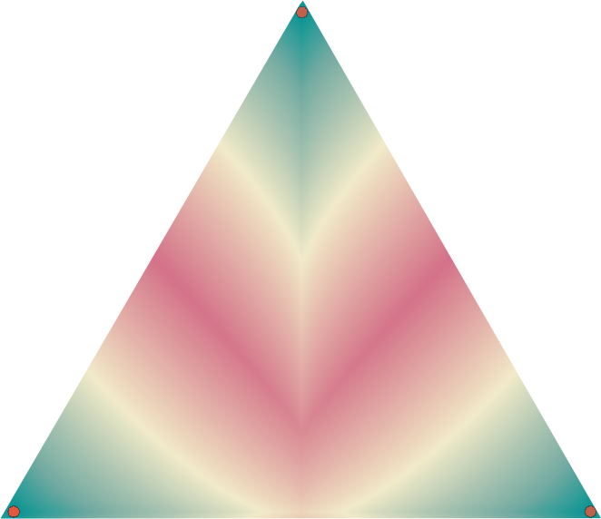
In other words, we suggest constraining a $Q$ model to behave in a way such that, as it becomes more certain in how it draws its predictions, the probability of drawing a “bad” partition converges to be no worse than the one of the simple model. The functional $\delta$ measures the uncertainty of $Q$ , and is considered as one of the design choices in the modeling of $Q$ . In turn, it will be used to bound the equivariance approximation error. Fig. 1 illustrates the qualitative behavior of $\delta$ .

We defer the discussion on how we provide a model for $Q$ supporting these ideas for later. Instead, we start by describing how $Q_{{\bm{Z}}|{\bm{X}}}$ is incorporated to model a piecewise equivariant layer.

Fixed partition.

To facilitate discussion, we first assume that ${\bm{Z}}$ is fixed, and we will start by describing a piecewise $E(d)$ equivariant layer with respect to ${\bm{Z}}$ partition. Let $G=E(d)\times\cdots\times E(d)$ be the product consisting of $k$ copies of the Euclidean motions group. For $g=(g_{1}\cdots,g_{k})\in G$ , we define

g\cdot({\bm{X}},{\bm{Z}})=\sum_{j=1}^{k}\left(g_{j}\cdot{\bm{X}}\right)\odot({\bm{Z}}{\bm{e}}_{j}\mathbf{1}_{d}^{T}),

(5)

where $g_{j}\cdot{\bm{X}}={\bm{X}}{\bm{R}}_{j}^{T}+\mathbf{1}_{n}{\bm{t}}_{j}^{T}$ , $\left\{{\bm{e}}_{j}\right\}_{j=1}^{k}$ is the standard basis in $\mathbb{R}^{k}$ , ${\bm{1}}_{d}$ is the vector of all ones in $\mathbb{R}^{d}$ , and $\odot$ denotes the Hadamard product between two matrices.

One appealing way to model a piecewise $E(d)$ equivariant function, $\psi:U\times\left\{0,1\right\}^{n\times k}\rightarrow U^{\prime}$ , which also respects the inherited order symmetry of the part’s assignments, is by employing an $E(d)$ -equivariant backbone $\psi_{b}:U\rightarrow U^{\prime}$ shared among the parts (Atzmon et al., 2022; Deng et al., 2023), taking the form:

\psi({\bm{X}},{\bm{Z}})=\sum_{j=1}^{k}\psi_{b}({\bm{X}}\odot{\bm{Z}}{\bm{e}}_{j}{\bm{1}}_{d}^{T})\odot{\bm{Z}}{\bm{e}}_{j}{\bm{1}}^{T}.

(6)

The following lemma, whose proof can be found in the Appendix, verifies these properties for $\psi$ .

Lemma 1.

Let $\psi:U\times\left\{0,1\right\}^{n\times k}\rightarrow U^{\prime}$ be a function as in Eq. (6). Let $g\in G$ and $\sigma_{k}(\cdot)$ a permutation on $[k]$ . Then,

	$\displaystyle\psi(g\cdot({\bm{X}},{\bm{Z}}),{\bm{Z}})$	$\displaystyle=g\cdot(\psi({\bm{X}},{\bm{Z}}),{\bm{Z}}),$
	$\displaystyle\psi({\bm{X}},{\bm{Z}}^{\prime})$	$\displaystyle=\psi({\bm{X}},{\bm{Z}})$

for any ${\bm{X}}\in U$ , ${\bm{Z}}\in\left\{0,1\right\}^{n\times k}$ , and ${\bm{Z}}^{\prime}={\bm{Z}}_{:,\sigma(i)}$ .

Note that one can consider augmenting the design of Eq. (6) with a function over orderless representation of parts $E(d)$ invariant features (Maron et al., 2020). Equipped with the construction in Eq. (6), we will now move on to the case where ${\bm{Z}}$ is uncertain.

Uncertain partition.

Incorporating ${Q_{{\bm{Z}}|{\bm{X}}}}$ into a layer can be done by marginalizing over the possible ${\bm{Z}}$ . Some simple options for marginalization are i) $\phi_{\textup{I}}({\bm{X}})=\psi({\bm{X}},\mathbb{E}_{Q}{\bm{Z}})$ as implemented in Atzmon et al. (2022); ii) $\phi_{\textup{II}}({\bm{X}})=\mathbb{E}_{Q}\psi({\bm{X}},{\bm{Z}})$ ; and iii) $\phi_{\textup{III}}({\bm{X}})=\psi\left({\bm{X}},{\bm{Z}}_{*}\right)$ , where $({\bm{Z}}_{*})_{i,:}={\bm{e}}_{\operatorname*{arg\,max}_{j}Q({\bm{Z}}|{\bm{X}})_{ij}}$ . Unfortunately, however, all of these options are merely an approximation of a piecewise $E(d)$ equivariant function. The scheme $\phi_{\textup{I}}$ relies on scaling, which can be an arbitrarily bad approximation to the input’s geometry. The scheme $\phi_{\textup{II}}$ relies on the averaging of equivariant point features, which is not stable under a realization of a particular partition ${\bm{Z}}\sim Q$ . Similarly, $\phi_{\textup{III}}$ is also not equivariant under all possible realizations of ${\bm{Z}}$ . However, the equivariance approximation error $\phi_{\textup{III}}$ induces can be controlled, as we discuss next.

Bounding the equivariant approximation error.

In this work, we advocate for layers of the form $\phi_{\textup{III}}$ . The motivation for doing so is that it enables a uniform control over the equivariant approximation error as a function of $Q$ , crucially, without relying on bounding the variation of $\phi$ . This advantage is especially prominent for neural networks, as existing techniques for bounding network’s bounded variation, e.g., by controlling the network’s Lipshitz constant, impose additional complexity to the network architecture and may hinder the training process (Anil et al., 2019). On the other hand, as we will see in the next section, the approximation error $Q$ induces can be controlled explicitly by a choice of hyper-parameters in the parametrization of $Q$ .

The next definition captures our suggested characterization for an approximation error of a desired piecewise $E(d)$ equivariant layer:

Definition 1.

Let $\phi:U\rightarrow U^{\prime}$ be a bounded function with $\left\|\phi\right\|\leq M$ . Let $\delta:(\Sigma_{k})^{n}\rightarrow\mathbb{R}_{+}$ , satisfying Eq. (3) and Eq. (4) w.r.t. $Q$ . Then, $\phi$ is a $(G,Q)$ equivariant function if and only if for any given ${\bm{X}}\in U$ , the following is satisfied

\mathbb{E}_{Q_{{\bm{Z}}|{\bm{X}}}}\left\|\phi\left(g\cdot({\bm{X}},{\bm{Z}})\right)-g\cdot(\phi({\bm{X}}),{\bm{Z}})\right\|\leq\left(\lambda(Q_{\textrm{simple}})+\delta(Q)\right)M

(7)

for all $g\in G$ . We denote the set of $(G,Q)$ equivariant functions by $\mathcal{F}_{Q}$ .

The above characterization for the equivariance approximation error can be seen as resulting from two different sources of properties in the partition prediction model: (i) an intrinsic source, as captured by $\delta$ , which measures the uncertainty of the model $Q$ , and (ii) an extrinsic source, determined by a measure independent from $Q$ as captured by $\lambda$ . In addition, the above definition generalizes the notion of exact equivariant function classes. For instance, consider $\widehat{{\bm{Z}}}$ satisfying $\widehat{{\bm{Z}}}{\bm{e}}_{j}={\bm{1}}$ for some fixed $j$ ; setting $\delta\equiv 0$ yields that $\mathcal{F}_{Q}$ coincides with the class of global $E(d)$ equivariant functions.

To conclude this section, we verify in the following theorem that our construction of $\phi$ indeed falls under the suggested characterization of approximate piecewise $E(d)$ equivariant functions. Proof details are in the Appendix.

Theorem 1.

Let $\phi:U\rightarrow U^{\prime}$ be of the form

\phi({\bm{X}})=\sum_{j=1}^{k}\psi_{b}({\bm{X}}\odot{\bm{Z}}_{*}{\bm{e}}_{j}{\bm{1}}^{T}_{d})\odot{\bm{Z}}_{*}{\bm{e}}_{j}{\bm{1}}^{T},

(8)

where $({\bm{Z}}_{*})_{i,:}={\bm{e}}_{\operatorname*{arg\,max}_{j}Q({\bm{Z}}|{\bm{X}})_{ij}}$ , and $\psi_{b}:U\rightarrow U^{\prime}$ is an $E(d)$ equivariant backbone. Then,

\phi\in\mathcal{F}_{Q}.

2.3 Q Prediction

So far, we have treated $Q$ as a given input to the layer. In fact, we suggest that $Q$ results from a piecewise equivariant prediction of a prior layer. Exceptional is the first layer, for which $Q=Q_{\textrm{simple}}$ . Given a layer output of the form in Eq. (8), we will next describe how $Q^{\textrm{pred}}$ is inferred. Note that $Q$ still denotes the given input partition prediction model.

Modeling considerations.

As a first attempt, one might consider parametrizing $Q^{\textrm{pred}}$ as the $\mathrm{softmax}$ of a per-point $Q$ piecewise invariant layer prediction. However, this approach introduces several difficulties, causing it to be unfeasible. Firstly, it is unclear how to supervise $Q$ during training to predict good sub-partitions of the ground-truth partition. Secondly, network optimization could be tricky, since the domain of possible partition solutions has a high dimensional combinatorial structure, especially due to our design bias for a large number of parts in early network layers. Lastly, there is a need to model the merging of parts in the input partition to generate a coarser one.

To address these challenges, we propose a geometric approach to model $Q^{\textrm{pred}}$ . Our suggestion is to set $Q^{\textrm{pred}}$ as the assignment scores resulting from the partitioning (i.e., clustering) in $R^{d}$ of $Q$ piecewise equivariant per-point predictions. Notably, this suggestion falls under the well-known attention layer (Vaswani et al., 2017; Locatello et al., 2020; Liu et al., 2023) following a query, key, and value structure with $\phi({\bm{X}})$ being the values and queries, part centers being the keys, and the prediction $Q^{\textrm{pred}}$ is proportional to the matching score of a query to a key. One of the advantages of this approach is that $Q^{\textrm{pred}}$ emerges as an orderless prediction with respect to possible parts assignments, thus simplifying the optimization domain. However, it is not clear how this model can (i) control the resulting $\delta(Q^{\textrm{pred}})$ by means of its design; and (ii) support the merging of parts to constitute a prediction of a coarser partition. To this end, we suggest that the part center (keys) predictions are set as the minimizers of an energy that is invariant to $Q$ piecewise $E(d)$ deformations of $\phi({\bm{X}})$ (values). We formalize this idea in the next paragraph.

Q Prediction.

Let ${\bm{Y}}=[{\bm{y}}_{1},\cdots,{\bm{y}}_{n}]^{T}\in\mathbb{R}^{n\times d}$ denote the first equivariant per-point prediction in $\phi({\bm{X}})\in U^{\prime}$ . Let $\left[{\bm{\mu}}^{*}_{j}\right]_{j=1}^{k}\in\mathbb{R}^{d\times k}$ denote the underlying predicted part centers with which the score of $Q^{\textrm{pred}}$ is defined. We define $\left[{\bm{\mu}}^{*}_{j}\right]_{j=1}^{k}$ as the minimizers of an energy consisting of the negative log-likelihood of a Gaussian Mixture Model and a regularization term that constraints the KL distance between all pairs of Gaussians to be greater than some threshold. Let $P({\bm{Y}};{\bm{\alpha}}=({\bm{\mu}}_{j},\pi_{j};\sigma)_{j=1}^{k})$ denote the mixture distribution, parametrized by ${\bm{\alpha}}$ . Then, the log-likelihood is $\log P({\bm{Y}};{\bm{\alpha}})=\sum_{i=1}^{n}\log(\sum_{j=1}^{k}\pi_{j}\mathcal{N}\left({\bm{y}}_{i};{\bm{\mu}}_{j},\sigma)\right)$ where $\mathcal{N}(\cdot;{\bm{\mu}}_{j},\sigma)$ denotes the density of an isotropic Gaussian random variable, centered at ${\bm{\mu}}_{j}$ with variance $\sigma^{2}I$ . Note that $\sigma$ is fixed and is considered as a hyper-parameter. Then, $\left[{\bm{\mu}}^{*}_{j}\right]_{j=1}^{k}$ are defined as

({\bm{\mu}}^{*}_{j},\pi^{*}_{j})=\operatorname*{arg\,min}_{\bm{\alpha}}-\log P({\bm{Y}};{\bm{\alpha}})-\tau\sum_{j\neq j^{\prime}}\pi_{j}\pi_{j}^{\prime}\log D_{\mathrm{KL}}(\mathcal{N}(\cdot;{\bm{\mu}}_{j})||\mathcal{N}(\cdot;{\bm{\mu}}_{j}^{\prime})).

(9)

In turn, the prediction $Q^{\textrm{pred}}_{ij}$ is defined as

Q^{\textrm{pred}}_{ij}=\frac{\mathcal{N}({\bm{y}}_{i};{\bm{\mu}}^{*}_{j},\sigma)\pi^{*}_{j}}{\sum_{j=1}^{k}\mathcal{N}({\bm{y}}_{i};{\bm{\mu}}^{*}_{j},\sigma)\pi^{*}_{j}}.

(10)

Importantly, the above construction yields that as $\sigma\rightarrow 0$ : i) $\lambda(Q^{\textrm{pred}})\rightarrow\lambda(Q_{\textrm{simple}})$ since each random partition is a minimizer of the likelihood functional, and ii) $\delta(Q^{\textrm{pred}})\rightarrow 0$ . In addition, $\sigma$ also controls the sensitivity of Gaussians to merge (under a fixed coefficient $\tau)$ , where larger values encourage Gaussians to explain wider distribution of values ${\bm{y}}_{i}$ . Thus, setting an increasing sequence of $\sigma$ values across layers supports the gradual coarsening of partitions design. Lastly, note that differentiating the prediction of $Q^{\textrm{pred}}$ w.r.t. its inputs is not trivial; these details are covered in the next section.

2.4 Implementation Details

Network architecture.

We start by sharing the details about the construction of the layer $\psi$ in Eq. (6) given a known partition ${\bm{Z}}$ . For that end, we used Frame Averaging (FA) (Puny et al., 2022) with a shared pointnet (Qi et al., 2017) network, $\tilde{\psi}$ . We define our shared equivariant backbone by

\psi_{b}({\bm{X}}\odot{\bm{Z}}{\bm{e}}_{j}{\bm{1}}^{T}_{d})=\left\langle\tilde{\psi}({\bm{X}}\odot{\bm{Z}}{\bm{e}}_{j}{\bm{1}}^{T}_{d})\right\rangle_{F({\bm{X}}\odot{\bm{Z}}{\bm{e}}_{j}{\bm{1}}^{T}_{d})}

where $F({\bm{X}}\odot{\bm{Z}}{\bm{e}}_{j}{\bm{1}}^{T}_{d})$ is the same PCA based construction for an $E(d)$ frame suggested in Puny et al. (2022), and $\left\langle\cdot\right\rangle$ is the FA symmetrization operator. Then, $\psi({\bm{X}},{\bm{Z}})$ is defined exactly as in Eq. (6). Since this construction needs to support layers with a relatively large number of parts $k$ , we implement the network $\psi_{b}$ using the sparse linear layers from Choy et al. (2019).

In all our experiments, we implemented the encoder as a composition of $L$ layers, $\textit{e}=\phi_{L}\circ\cdots\circ\phi_{1}$ , with $L=4$ ; see Fig. 2. $Q_{\textrm{simple}}$ is set as the input to $\phi_{1}$ . In fact, $Q_{\textrm{simple}}$ can be further regulated than the naive suggestion. In practice, we set $Q_{\textrm{simple}}$ by a Voronoi partition resulting from $k$ furthest point samples from the input ${\bm{X}}$ . The exact analysis of $\lambda(Q_{\textrm{simple}})$ as a function of $n$ and $k$ is out of the scope of this work – we only rely on Eq. (4).

Q prediction.

For finding a minimizer of Eq. (9), we used a slight modification of the well-known EM algorithm (Dempster et al., 1977) that supports the merging of centers closer than the threshold $\tau$ . Note that during training, the backward calculation requires the derivative of $\frac{\partial{Q}}{\partial\phi}$ . Since the EM is in an iterative algorithm, this might unnecessarily increase the computational graph of the backward computation. To mitigate this, we use the following construction, based on implicit differentiation (Atzmon et al., 2019; Bai et al., 2019). Let $\tilde{{\bm{\alpha}}}$ be a minimizer Eq. (9) that is detached from the computational graph and ${\bm{Y}}$ . Then, $s({\bm{Y}};\tilde{{\bm{\alpha}}})=0$ where $s({\bm{Y}};\tilde{{\bm{\alpha}}})=\nabla_{{\bm{\alpha}}}\log P({\bm{Y}};{\bm{\alpha}})$ , known in the literature as the score function (Bishop & Nasrabadi, 2006). We define

{\bm{\alpha}}=\tilde{{\bm{\alpha}}}+I^{-1}\left(\tilde{{\bm{\alpha}}}\right)s\left({\bm{Y}};\tilde{{\bm{\alpha}}}\right),

(11)

where $I^{-1}(\tilde{{\bm{\alpha}}})=\mathrm{Var}\left(s({\bm{Y}};\tilde{{\bm{\alpha}}})\right)$ is the fisher information matrix (Bishop & Nasrabadi, 2006) calculated at $\tilde{{\bm{\alpha}}}$ . Importantly, $I$ only depends on $s$ and does not involve second derivative calculations. It can be easily verified that ${\bm{\alpha}}$ is a minimizer of Eq. (9) and that $\frac{\partial{{\bm{\alpha}}}}{\partial{{\bm{Y}}}}=\frac{\partial{\left(\operatorname*{arg\,min}_{{\bm{\alpha}}}(E({\bm{\alpha}},{\bm{Y}}))\right)}}{\partial{{\bm{Y}}}}$ , where $E(\cdot)$ denotes the energy defined in Eq. (9). This is summarized in Alg. 1, found in the Appendix.

Training details.

Our framework requires supervision in order to train $Q^{\textrm{pred}}$ to approximate the ground-truth partition. To that end, we compute the ground-truth ${\bm{Y}}_{\textrm{GT}}\in\mathbb{R}^{n\times d}$ to supervise the parts center vote predictions ${\bm{Y}}_{l}\in\mathbb{R}^{n\times d}$ of the $l^{\text{th}}$ layer. We utilize the given segmentation information, to calculate ${\bm{Y}}_{\textrm{GT}}={\bm{Z}}{\bm{C}}^{T}-{\bm{X}}$ , where ${\bm{Z}}\in\left\{0,1\right\}^{n\times k}$ are the ground-truth assignments of ${\bm{X}}\in\mathbb{R}^{n\times d}$ and ${\bm{C}}\in\mathbb{R}^{d\times k}$ is calculated as the center of the minimal bounding box encompassing each of the input parts. Then, a standard $L_{1}$ loss is added to optimization,

\mathrm{loss}_{\textrm{A}}=\sum_{l=1}^{L}\left\|{\bm{Y}}_{l}-{\bm{Y}}_{\textrm{GT}}\right\|.

3 Experiments

We evaluate our method on two types of datasets that fit piecewise $E(3)$ symmetry: (i) scans of human subjects performing various sequences of movements (Loper et al., 2015; Bogo et al., 2017; Mahmood et al., 2019), and (ii) real-world rooms scans of furniture-type objects (Huang et al., 2021a). In all of our experiments, we used the ground-truth segmentation maps to extract ${\bm{Y}}_{\textrm{GT}}$ supervision as described in Sec. 2.4.

3.1 Human Scans

We start by evaluating our framework for the task of point part segmentation, a basic computer-vision task with many downstream applications. Specifically, we consider human body parts segmentation, where the goal is to assign each of the input scan points to a part chosen from a predefined list. In our case, the list consists of $24$ body parts.

To evaluate different aspects of our framework, we use three different train/test splits. The first consists of a random ( $90\%/10\%$ ) train/test split of $41,461$ human models from the SMPL dataset (Loper et al., 2015) consisting of $10$ different human subjects as in (Huang et al., 2021b). This experiment acts as a sanity test and ensure our method does not underperform compared to baselines. The second and third splits use the scans from the Dynamic FAUST (DFAUST) dataset (Bogo et al., 2017), consisting of $10$ to $12$ different sequences of motions (e.g., jumping jacks, punching, etc.) for each of the $10$ human subjects. In the second split, we divide the data by a random choice of a different action sequences for each human. This experiment ensures our method can generalize knowledge of action sequences seen in training from one human subject to other human subjects at test time. Finally, in the third split we choose the same sequence of movements (e.g., the one-leg jump sequence) to be removed from the training set and be placed as the test set. The last test evaluates the effect of the piecewise $E(3)$ prior, as implemented in our method, to generalize to unseen movement.

Method random unseen random seq. unseen seq. PointNet

84.4

78.5

80.1

DGCNN

82.2

70.3

79.5

42.4

24.8

33.3

VN-T

63.5

50.9

50.0

83.5

78.1

76.7

EPN

89.6

77.8

84.1

Ours 94.2 92.2 93.5

Table 1: Mean IoU(%) test set score for human body parts segmentation.

In Tab. 1, we report the mean IoU(%) score for all $3$ tests. As baseline models, we opt for PointNet (Qi et al., 2017) and DGCNN (Wang et al., 2019) as order invariant point networks. For $E(3)$ invariant networks, our baselines selection includes Vector Neurons (VN) (Deng et al., 2021), VN-Transformer (VN-T) (Assaad et al., 2023), FrameAveraging (FA) (Puny et al., 2022), and Equivariant Point Network (EPN) (Chen et al., 2021) backbone as implemented in the human body part segmentation network described in Feng et al. (2023). Fig. 4 shows qualitative test results of an unseen random seq. pose (first row) and an unseen random pose (second row). We conclude from the results that (i) our framework is a valid backbone with similar expressive power as common point network baselines, (ii) our framework utilizes piecewise $E(3)$ equivariance to gain better generalization across human subjects than baseline approaches and, (iii) piecewise $E(3)$ equivariant prior can help to generalize to unseen movements.

Lastly, to test the versatility of our framework, we evaluate it on a point cloud classification task. On that hand, we consider the DFaust subset of AMASS (Mahmood et al., 2019), consisting of $9$ human subjects. We define the task of classifying a model to a subject. For testing, we use an "out of distribution" test set from PosePrior (Akhter & Black, 2015). The results from this experiment support the usability of our framework for classification tasks as well. The detailed report can be found in the Appendix, including all the hyper-parameters used for the experiments in this section.

3.2 Room Scans

In this section, we test the potential of our framework for one-shot generalization. To that end, we employ a dataset of $8$ scenes capturing a real-world room where the furniture in the room has been positioned differently in each of the 8 scans for each scene. Within each scan, there are $3$ to $4$ labeled furniture-type objects, including the floor. The task objective is to assign each input point to one of the object instances composing the scene. In addition to the difficulty of segmenting moving objects in the scene, solutions to this task must handle noise and sampling artifacts arising from the scanning procedure. For instance, scans of objects occasionally contain holes or exhibit ghost geometry. Here we compare two alternative solutions this this task: (1) we only train our method using a single scan, and test its generalization to the other seven scans of the same scene. (2) We train baseline networks on the large-scale synthetic shape segmentation dataset from Huang et al. (2021a), which randomly samples independent motions for multiple objects taken from ShapeNet (Chang et al., 2015).

In Tab. 2 we report the mean IoU(%) test score for each of the scenes. Fig. 3 shows qualitative results for $2$ rooms. Despite only training on a single scan, our model outperforms baselines trained on a large synthetic dataset in 7 out of the 8 test scenes. These results suggest potential advantages of using piecewise $E(3)$ equivariant architectures in a single shot setting over the use of large-scale synthetic data. Furthermore, to make baseline approaches work, we employed a RANSAC algorithm to identify the ground plane, with an inlier distance threshold of $0.02$ and $1000$ RANSAC iterations. In contrast, our method requires no preprocessing since the network can treat the floor as it would for any other part of the input data.

Method	Scene $1$	Scene $2$	Scene $3$	Scene $4$	Scene $5$	Scene $6$	Scene $7$	Scene $8$
PointNet	$33.0\pm 8.5$	$50.2\pm 4.3$	$31.1\pm 3.4$	$38.3\pm 4.3$	$36.7\pm 6.1$	$45.2\pm 22.0$	$57.4\pm 1.5$	$36.6\pm 4.6$
DGCNN	$36.7\pm 3.6$	$38.8\pm 10.8$	$41.8\pm 4.9$	$31.0\pm 2.7$	$48.9\pm 4.3$	$35.1\pm 8.4$	$59.5\pm 7.3$	$35.4\pm 6.3$
VN	$13.0\pm 2.8$	$18.6\pm 1.5$	$24.7\pm 0.8$	$15.2\pm 1.1$	$24.4\pm 1.1$	$17.6\pm 1.7$	$25.6\pm 1.0$	$23.0\pm 1.2$
Ours	$\textbf{88.0}\pm 13.0$	$\textbf{98.2}\pm 0.7$	$\textbf{97.4}\pm 1.5$	$\textbf{96.3}\pm 2.0$	$\textbf{93.2}\pm 3.9$	$93.4\pm 2.8$	$\textbf{83.3}\pm 13.3$	$\textbf{92.2}\pm 1.8$
PointNet (Synthteic)	$76.6\pm 22.4$	$97.3\pm 2.1$	$91.2\pm 4.8$	$89.7\pm 4.0$	$91.9\pm 5.1$	$95.1\pm 1.0$	$66.6\pm 9.7$	$83.2\pm 4.0$
DGCNN (Synthetic)	$77.5\pm 22.3$	$93.7\pm 10.9$	$97.1\pm 0.7$	$84.4\pm 13.0$	$89.1\pm 16.6$	$\mathbf{95.6}\pm 1.1$	$76.2\pm 10.6$	$90.6\pm 6.2$
VN (Synthteic)	$65.5\pm 18.7$	$93.7\pm 4.9$	$80.7\pm 17.6$	$59.3\pm 11.0$	$92.5\pm 4.9$	$82.5\pm 15.0$	$77.4\pm 6.1$	$62.0\pm 12.9$

Table 2: One-shot generalization on real-world scans from the Dynlab dataset (Huang et al., 2021a).

4 Related work

Global Equivariance.

We introduce a novel method for piecewise $E(3)$ equivariance in point networks. Euclidean group symmetry has been studied in point networks mainly in describing architectures that accommodate global transformations (Chen et al., 2019; Thomas et al., 2018; Fuchs et al., 2020; Chen et al., 2021; Deng et al., 2021; Assaad et al., 2023; Zisling & Sharf, 2022; Katzir et al., 2022; Poulenard & Guibas, 2021; Puny et al., 2022). These was shown to perform well in various applications including reconstruction (Deng et al., 2021; Chatzipantazis et al., 2022; Chen et al., 2022), pose estimation (Li et al., 2021; Lin et al., 2023; Pan et al., 2022; Sajnani et al., 2022; Zhu et al., 2022), and robot manipulation (Simeonov et al., 2022; Higuera et al., 2023; Xue et al., 2023) tasks. Some works have dealt with respecting the symmetry by manipulating their input representation (Deng et al., 2018; Zhang et al., 2019; Gojcic et al., 2019). A popular line of work utilizes the theory of spherical harmonics to achieve equivariance (Worrall et al., 2017; Esteves et al., 2018; Liu et al., 2018; Weiler et al., 2018; Cohen et al., 2018).

Object-Level and Part-Based Equivariance

Several works have studied the equivariance of parts. EON (Yu et al., 2022) and EFEM (Lei et al., 2023) both studied object-level equivariance in scenes. EON used a manually tuned ‘suspension’ to compute an equivariant object frame in which the context is aggregated. In EFEM, instance segmentation is achieved by training a shape prior using a shape collection, and employing it to refine scene regions. Instead, we do not assume prior knowledge of the underlying partition. Equivariance for per-part pose estimation in articulated shape was devised in Liu et al. (2023). Yet their self-supervised approach relies on part grouping according to features that are invariant to global rotations which may result in unknown errors when local transformations are introduced. Part-based equivariance was also studied for segmentation in Deng et al. (2023), relying on an intriguing fixed-point convergence procedure.

5 Conclusion

We presented APEN, a point network design for approximately piecewise $E(3)$ equivariant models. We implemented APEN networks to tackle recognition tasks such as point cloud segmentation, and classification, demonstrating superior generalization over common baselines. On the theoretical side, our work lays the ground for an analysis of piecewise equivariant networks in terms of their equivariance approximation error. The bounds we present in this study serve as merely initial insights on the possibility of controlling the equivariance approximation error, and further analysis of our suggested bounds is marked as an interesting future work. Further extending this framework for other 3D tasks, e.g., generative modeling and reconstruction is another interesting research venue.

Acknowledgments

The authors would like to thank Jonah Philion for the insightful discussions and valuable comments. Or Litany is a Taub fellow and is supported by the Azrieli Foundation Early Career Faculty Fellowship.

References

Akhter & Black (2015) Ijaz Akhter and Michael J Black. Pose-conditioned joint angle limits for 3d human pose reconstruction. In Proceedings of the IEEE conference on computer vision and pattern recognition, pp. 1446–1455, 2015.
Anil et al. (2019) Cem Anil, James Lucas, and Roger Grosse. Sorting out lipschitz function approximation. In International Conference on Machine Learning, pp. 291–301. PMLR, 2019.
Assaad et al. (2023) Serge Assaad, Carlton Downey, Rami Al-Rfou, Nigamaa Nayakanti, and Ben Sapp. Vn-transformer: Rotation-equivariant attention for vector neurons, 2023.
Atzmon et al. (2019) Matan Atzmon, Niv Haim, Lior Yariv, Ofer Israelov, Haggai Maron, and Yaron Lipman. Controlling neural level sets. Advances in Neural Information Processing Systems, 32, 2019.
Atzmon et al. (2022) Matan Atzmon, Koki Nagano, Sanja Fidler, Sameh Khamis, and Yaron Lipman. Frame averaging for equivariant shape space learning. In Proceedings of the IEEE/CVF Conference on Computer Vision and Pattern Recognition, pp. 631–641, 2022.
Bai et al. (2019) Shaojie Bai, J Zico Kolter, and Vladlen Koltun. Deep equilibrium models. Advances in Neural Information Processing Systems, 32, 2019.
Bietti et al. (2021) Alberto Bietti, Luca Venturi, and Joan Bruna. On the sample complexity of learning with geometric stability. arXiv preprint arXiv:2106.07148, 2021.
Bishop & Nasrabadi (2006) Christopher M Bishop and Nasser M Nasrabadi. Pattern recognition and machine learning, volume 4. Springer, 2006.
Bogo et al. (2017) Federica Bogo, Javier Romero, Gerard Pons-Moll, and Michael J. Black. Dynamic FAUST: Registering human bodies in motion. In IEEE Conf. on Computer Vision and Pattern Recognition (CVPR), July 2017.
Chang et al. (2015) Angel X Chang, Thomas Funkhouser, Leonidas Guibas, Pat Hanrahan, Qixing Huang, Zimo Li, Silvio Savarese, Manolis Savva, Shuran Song, Hao Su, et al. Shapenet: An information-rich 3d model repository. arXiv preprint arXiv:1512.03012, 2015.
Chatzipantazis et al. (2022) Evangelos Chatzipantazis, Stefanos Pertigkiozoglou, Edgar Dobriban, and Kostas Daniilidis. Se (3)-equivariant attention networks for shape reconstruction in function space. arXiv preprint arXiv:2204.02394, 2022.
Chen et al. (2019) Chao Chen, Guanbin Li, Ruijia Xu, Tianshui Chen, Meng Wang, and Liang Lin. Clusternet: Deep hierarchical cluster network with rigorously rotation-invariant representation for point cloud analysis. In Proceedings of the IEEE/CVF conference on computer vision and pattern recognition, pp. 4994–5002, 2019.
Chen et al. (2021) Haiwei Chen, Shichen Liu, Weikai Chen, Hao Li, and Randall Hill. Equivariant point network for 3d point cloud analysis. In Proceedings of the IEEE/CVF conference on computer vision and pattern recognition, pp. 14514–14523, 2021.
Chen et al. (2022) Yunlu Chen, Basura Fernando, Hakan Bilen, Matthias Nießner, and Efstratios Gavves. 3d equivariant graph implicit functions. In European Conference on Computer Vision, pp. 485–502. Springer, 2022.
Choy et al. (2019) Christopher Choy, JunYoung Gwak, and Silvio Savarese. 4d spatio-temporal convnets: Minkowski convolutional neural networks. In Proceedings of the IEEE/CVF conference on computer vision and pattern recognition, pp. 3075–3084, 2019.
Cohen et al. (2018) Taco S Cohen, Mario Geiger, Jonas Köhler, and Max Welling. Spherical cnns. arXiv preprint arXiv:1801.10130, 2018.
Dempster et al. (1977) Arthur P Dempster, Nan M Laird, and Donald B Rubin. Maximum likelihood from incomplete data via the em algorithm. Journal of the royal statistical society: series B (methodological), 39(1):1–22, 1977.
Deng et al. (2021) Congyue Deng, Or Litany, Yueqi Duan, Adrien Poulenard, Andrea Tagliasacchi, and Leonidas J Guibas. Vector neurons: A general framework for so (3)-equivariant networks. In Proceedings of the IEEE/CVF International Conference on Computer Vision, pp. 12200–12209, 2021.
Deng et al. (2023) Congyue Deng, Jiahui Lei, Bokui Shen, Kostas Daniilidis, and Leonidas Guibas. Banana: Banach fixed-point network for pointcloud segmentation with inter-part equivariance. arXiv preprint arXiv:2305.16314, 2023.
Deng et al. (2018) Haowen Deng, Tolga Birdal, and Slobodan Ilic. Ppf-foldnet: Unsupervised learning of rotation invariant 3d local descriptors. In Proceedings of the European conference on computer vision (ECCV), pp. 602–618, 2018.
Elesedy & Zaidi (2021) Bryn Elesedy and Sheheryar Zaidi. Provably strict generalisation benefit for equivariant models. In International Conference on Machine Learning, pp. 2959–2969. PMLR, 2021.
Esteves et al. (2018) Carlos Esteves, Christine Allen-Blanchette, Ameesh Makadia, and Kostas Daniilidis. Learning so (3) equivariant representations with spherical cnns. In Proceedings of the European Conference on Computer Vision (ECCV), pp. 52–68, 2018.
Feng et al. (2023) Haiwen Feng, Peter Kulits, Shichen Liu, Michael J Black, and Victoria Fernandez Abrevaya. Generalizing neural human fitting to unseen poses with articulated se (3) equivariance. In Proceedings of the IEEE/CVF International Conference on Computer Vision, pp. 7977–7988, 2023.
Fuchs et al. (2020) Fabian Fuchs, Daniel Worrall, Volker Fischer, and Max Welling. Se (3)-transformers: 3d roto-translation equivariant attention networks. Advances in neural information processing systems, 33:1970–1981, 2020.
Gojcic et al. (2019) Zan Gojcic, Caifa Zhou, Jan D Wegner, and Andreas Wieser. The perfect match: 3d point cloud matching with smoothed densities. In Proceedings of the IEEE/CVF conference on computer vision and pattern recognition, pp. 5545–5554, 2019.
Higuera et al. (2023) Carolina Higuera, Siyuan Dong, Byron Boots, and Mustafa Mukadam. Neural contact fields: Tracking extrinsic contact with tactile sensing. In 2023 IEEE International Conference on Robotics and Automation (ICRA), pp. 12576–12582. IEEE, 2023.
Huang et al. (2021a) Jiahui Huang, He Wang, Tolga Birdal, Minhyuk Sung, Federica Arrigoni, Shi-Min Hu, and Leonidas J Guibas. Multibodysync: Multi-body segmentation and motion estimation via 3d scan synchronization. In Proceedings of the IEEE/CVF Conference on Computer Vision and Pattern Recognition, pp. 7108–7118, 2021a.
Huang et al. (2021b) Qixing Huang, Xiangru Huang, Bo Sun, Zaiwei Zhang, Junfeng Jiang, and Chandrajit Bajaj. Arapreg: An as-rigid-as possible regularization loss for learning deformable shape generators. In Proceedings of the IEEE/CVF international conference on computer vision, pp. 5815–5825, 2021b.
Katzir et al. (2022) Oren Katzir, Dani Lischinski, and Daniel Cohen-Or. Shape-pose disentanglement using se (3)-equivariant vector neurons. In European Conference on Computer Vision, pp. 468–484. Springer, 2022.
Kingma & Ba (2014) Diederik P Kingma and Jimmy Ba. Adam: A method for stochastic optimization. arXiv preprint arXiv:1412.6980, 2014.
Lei et al. (2023) Jiahui Lei, Congyue Deng, Karl Schmeckpeper, Leonidas Guibas, and Kostas Daniilidis. Efem: Equivariant neural field expectation maximization for 3d object segmentation without scene supervision, 2023.
Li et al. (2021) Xiaolong Li, Yijia Weng, Li Yi, Leonidas Guibas, A. Lynn Abbott, Shuran Song, and He Wang. Leveraging se(3) equivariance for self-supervised category-level object pose estimation, 2021.
Lin et al. (2023) Cheng-Wei Lin, Tung-I Chen, Hsin-Ying Lee, Wen-Chin Chen, and Winston H Hsu. Coarse-to-fine point cloud registration with se (3)-equivariant representations. In 2023 IEEE International Conference on Robotics and Automation (ICRA), pp. 2833–2840. IEEE, 2023.
Liu et al. (2018) Min Liu, Fupin Yao, Chiho Choi, Ayan Sinha, and Karthik Ramani. Deep learning 3d shapes using alt-az anisotropic 2-sphere convolution. In International Conference on Learning Representations, 2018.
Liu et al. (2023) Xueyi Liu, Ji Zhang, Ruizhen Hu, Haibin Huang, He Wang, and Li Yi. Self-supervised category-level articulated object pose estimation with part-level se(3) equivariance, 2023.
Locatello et al. (2020) Francesco Locatello, Dirk Weissenborn, Thomas Unterthiner, Aravindh Mahendran, Georg Heigold, Jakob Uszkoreit, Alexey Dosovitskiy, and Thomas Kipf. Object-centric learning with slot attention. Advances in Neural Information Processing Systems, 33:11525–11538, 2020.
Loper et al. (2015) Matthew Loper, Naureen Mahmood, Javier Romero, Gerard Pons-Moll, and Michael J. Black. SMPL: A skinned multi-person linear model. ACM Trans. Graphics (Proc. SIGGRAPH Asia), 34(6):248:1–248:16, October 2015.
Mahmood et al. (2019) Naureen Mahmood, Nima Ghorbani, Nikolaus F Troje, Gerard Pons-Moll, and Michael J Black. Amass: Archive of motion capture as surface shapes. In Proceedings of the IEEE/CVF international conference on computer vision, pp. 5442–5451, 2019.
Maron et al. (2020) Haggai Maron, Or Litany, Gal Chechik, and Ethan Fetaya. On learning sets of symmetric elements. In International conference on machine learning, pp. 6734–6744. PMLR, 2020.
Pan et al. (2022) Haoran Pan, Jun Zhou, Yuanpeng Liu, Xuequan Lu, Weiming Wang, Xuefeng Yan, and Mingqiang Wei. So (3)-pose: So (3)-equivariance learning for 6d object pose estimation. In Computer Graphics Forum, volume 41, pp. 371–381. Wiley Online Library, 2022.
Paszke et al. (2019) Adam Paszke, Sam Gross, Francisco Massa, Adam Lerer, James Bradbury, Gregory Chanan, Trevor Killeen, Zeming Lin, Natalia Gimelshein, Luca Antiga, et al. Pytorch: An imperative style, high-performance deep learning library. Advances in neural information processing systems, 32:8026–8037, 2019.
Poulenard & Guibas (2021) Adrien Poulenard and Leonidas J Guibas. A functional approach to rotation equivariant non-linearities for tensor field networks. In Proceedings of the IEEE/CVF Conference on Computer Vision and Pattern Recognition, pp. 13174–13183, 2021.
Puny et al. (2022) Omri Puny, Matan Atzmon, Edward J. Smith, Ishan Misra, Aditya Grover, Heli Ben-Hamu, and Yaron Lipman. Frame averaging for invariant and equivariant network design. In International Conference on Learning Representations, 2022. URL https://openreview.net/forum?id=zIUyj55nXR.
Qi et al. (2017) Charles R Qi, Hao Su, Kaichun Mo, and Leonidas J Guibas. Pointnet: Deep learning on point sets for 3d classification and segmentation. In Proceedings of the IEEE conference on computer vision and pattern recognition, pp. 652–660, 2017.
Sajnani et al. (2022) Rahul Sajnani, Adrien Poulenard, Jivitesh Jain, Radhika Dua, Leonidas J Guibas, and Srinath Sridhar. Condor: Self-supervised canonicalization of 3d pose for partial shapes. In Proceedings of the IEEE/CVF Conference on Computer Vision and Pattern Recognition, pp. 16969–16979, 2022.
Simeonov et al. (2022) Anthony Simeonov, Yilun Du, Andrea Tagliasacchi, Joshua B Tenenbaum, Alberto Rodriguez, Pulkit Agrawal, and Vincent Sitzmann. Neural descriptor fields: Se (3)-equivariant object representations for manipulation. In 2022 International Conference on Robotics and Automation (ICRA), pp. 6394–6400. IEEE, 2022.
Tahmasebi & Jegelka (2023) Behrooz Tahmasebi and Stefanie Jegelka. The exact sample complexity gain from invariances for kernel regression on manifolds, 2023.
Thomas et al. (2018) Nathaniel Thomas, Tess Smidt, Steven Kearnes, Lusann Yang, Li Li, Kai Kohlhoff, and Patrick Riley. Tensor field networks: Rotation-and translation-equivariant neural networks for 3d point clouds. arXiv preprint arXiv:1802.08219, 2018.
Vaswani et al. (2017) Ashish Vaswani, Noam Shazeer, Niki Parmar, Jakob Uszkoreit, Llion Jones, Aidan N Gomez, Łukasz Kaiser, and Illia Polosukhin. Attention is all you need. Advances in neural information processing systems, 30, 2017.
Wang et al. (2019) Yue Wang, Yongbin Sun, Ziwei Liu, Sanjay E Sarma, Michael M Bronstein, and Justin M Solomon. Dynamic graph cnn for learning on point clouds. Acm Transactions On Graphics (tog), 38(5):1–12, 2019.
Weiler et al. (2018) Maurice Weiler, Mario Geiger, Max Welling, Wouter Boomsma, and Taco Cohen. 3d steerable cnns: Learning rotationally equivariant features in volumetric data, 2018.
Worrall et al. (2017) Daniel E Worrall, Stephan J Garbin, Daniyar Turmukhambetov, and Gabriel J Brostow. Harmonic networks: Deep translation and rotation equivariance. In Proceedings of the IEEE conference on computer vision and pattern recognition, pp. 5028–5037, 2017.
Xue et al. (2023) Zhengrong Xue, Zhecheng Yuan, Jiashun Wang, Xueqian Wang, Yang Gao, and Huazhe Xu. Useek: Unsupervised se (3)-equivariant 3d keypoints for generalizable manipulation. In 2023 IEEE International Conference on Robotics and Automation (ICRA), pp. 1715–1722. IEEE, 2023.
Yu et al. (2022) Hong-Xing Yu, Jiajun Wu, and Li Yi. Rotationally equivariant 3d object detection. In Proceedings of the IEEE International Conference on Computer Vision and Pattern Recognition, 2022.
Zaheer et al. (2017) Manzil Zaheer, Satwik Kottur, Siamak Ravanbakhsh, Barnabas Poczos, Ruslan Salakhutdinov, and Alexander Smola. Deep sets. arXiv preprint arXiv:1703.06114, 2017.
Zhang et al. (2019) Zhiyuan Zhang, Binh-Son Hua, David W Rosen, and Sai-Kit Yeung. Rotation invariant convolutions for 3d point clouds deep learning. In 2019 International conference on 3d vision (3DV), pp. 204–213. IEEE, 2019.
Zhu et al. (2022) Minghan Zhu, Maani Ghaffari, and Huei Peng. Correspondence-free point cloud registration with so (3)-equivariant implicit shape representations. In Conference on Robot Learning, pp. 1412–1422. PMLR, 2022.
Zisling & Sharf (2022) Hedi Zisling and Andrei Sharf. Vnt-net: Rotational invariant vector neuron transformers, 2022.

Appendix A Appendix

A.1 Proofs

A.1.1 Proof of Lemma 1

Proof.

(Lemma 1) Let ${\bm{X}}\in U$ , ${\bm{Z}}\in\{0,1\}^{n\times k}$ , and $g\in G$ . Then,

	$\displaystyle\psi(g\cdot({\bm{X}},{\bm{Z}}),{\bm{Z}})$	$\displaystyle=\sum_{j=1}^{k}\psi_{b}(g\cdot({\bm{X}},{\bm{Z}})\odot{\bm{Z}}{\bm{e}}_{j}{\bm{1}}_{d}^{T})\odot{\bm{Z}}{\bm{e}}_{j}{\bm{1}}^{T}=$
	$\displaystyle\sum_{j=1}^{k}\psi_{b}(\sum_{j=1}^{k}\left(g_{j}\cdot{\bm{X}}\right)\odot({\bm{Z}}{\bm{e}}_{j}\mathbf{1}_{d}^{T}))\odot{\bm{Z}}{\bm{e}}_{j}{\bm{1}}^{T}$	$\displaystyle=\sum_{j=1}^{k}g_{j}\cdot\psi_{b}({\bm{X}}\odot{\bm{Z}}{\bm{e}}_{j}\mathbf{1}_{d}^{T})\odot{\bm{Z}}{\bm{e}}_{j}{\bm{1}}^{T}$

where the last equality follows from the fact the $\psi_{b}$ is $E(d)$ equivariant and the second equality from the fact that ${\bm{Z}}{\bm{e}}_{j}\odot{\bm{Z}}{\bm{e}}_{j}^{\prime}={\bm{0}}$ for $j\neq j^{\prime}$ . Lastly, for any permutation $\sigma_{k}(\cdot)$ , we have,

\sum_{j=1}^{k}\psi_{b}({\bm{X}}\odot{\bm{Z}}{\bm{e}}_{\sigma_{k}(j)}{\bm{1}}_{d}^{T})\odot{\bm{Z}}{\bm{e}}_{\sigma_{k}(j)}{\bm{1}}^{T}=\sum_{j=1}^{k}\psi_{b}({\bm{X}}\odot{\bm{Z}}{\bm{e}}_{j)}{\bm{1}}_{d}^{T})\odot{\bm{Z}}{\bm{e}}_{j}{\bm{1}}^{T}

∎

A.1.2 Proof of Theorem 1

Proof.

(Theorem 1) Let $\phi:U\rightarrow U^{\prime}$ be of the form

\phi({\bm{X}})=\sum_{j=1}^{k}\psi_{b}({\bm{X}}\odot{\bm{Z}}_{*}{\bm{e}}_{j}{\bm{1}}^{T}_{d})\odot{\bm{Z}}_{*}{\bm{e}}_{j}{\bm{1}}^{T},

(12)

where $({\bm{Z}}_{*})_{i,:}={\bm{e}}_{\operatorname*{arg\,max}_{j}Q({\bm{Z}}|{\bm{X}})_{ij}}$ , and $\psi_{b}:U\rightarrow U^{\prime}$ is an $E(d)$ equivariant backbone.

Let $A=\left\{{\bm{Z}}\neq{\bm{Z}}_{*}\right\}$ . Then,

Q(A)\leq\sum_{i=1}^{n}(1-Q({\bm{e}}_{i}{\bm{Z}}={\bm{e}}_{i}{\bm{Z}}_{*}))=\sum_{i=1}^{n}(1-Q_{ij(i)_{*}})

where $j(i)_{*}=\operatorname*{arg\,max}_{j}Q_{ij}$ . Then, we set

\delta(Q)=\sum_{i=1}^{n}(1-Q_{ij(i)_{*}}).

Clearly $\delta$ satisfies conditon 3. Now, Let $Q$ satisfying condition 4 w.r.t. $\lambda$ . Let $B=\left\{{\bm{Z}}|\ \exists\ 1\leq i,j\leq n\text{ s.t. }\left({\bm{Z}}{\bm{Z}}^{T}\right)_{ij}>\left(\widehat{{\bm{Z}}}\widehat{{\bm{Z}}}^{T}\right)_{ij}\right\}$ . Then,

\left\{{\bm{Z}}\right\}=(B\cap A)\cup(B\cap A^{C})\cup(B^{C}\cap A)\cup(B^{C}\cap A^{C}).

Note that for $B^{C}\cap A^{C}$ there is no equivariance approximation error. For $(B\cap A)$ , and $(B^{C}\cap A)$ we can bound using $\delta(Q)$ . Lastly, ${\bm{Z}}\in(B\cap A^{C})$ means ${\bm{Z}}_{*}$ is a "bad" partition, thus $\lambda(Q)\leq\lambda(Q_{\textrm{simple}})$ . To conclude, we use a union bound composed of the decomposition above to get that,

\mathbb{E}_{Q_{{\bm{Z}}|{\bm{X}}}}\left\|\phi\left(g\cdot({\bm{X}},{\bm{Z}})\right)-g\cdot(\phi({\bm{X}}),{\bm{Z}})\right\|\leq(\lambda(Q_{\textrm{simple}})+\delta(Q))M.

∎

A.2 Q Prediction

In this section we provide an empirical validation to the expected behavior of $\lambda(Q_{\text{simple}})$ as $k\rightarrow n$ . To that end, we examine a 2D toy example, featuring $n=14$ points partitioned to $3$ groups. Figure 5 shows this toy example, with distinct colors denoting the ground truth partition. Figure 6 shows a plot of $\lambda(Q)$ values for $k\in[1,14]$ . The green line shows $\lambda(Q)$ for the simple $Q$ model, defined by a uniform draw of $k$ parts partition, where each part includes at least one point. The red line shows $\lambda(Q)$ for a $Q$ model, defined by a Voronoi partition with centers drawn randomly proportionally to $k$ furthest point sampling. Note that as expected, $\lambda(Q)\rightarrow 0$ as $k\rightarrow n$ .

Next, we provide in Alg. 1 a detailed description of our $Q$ prediction algorithm.

Algorithm 1 Q prediction

Input: ${\bm{Y}}$ ; $\tau>0$ merge threshold and $f$ merge frequency

i\leftarrow 0

({\bm{\mu}}_{j})\leftarrow\textit{random furthest point sample of }k\textit{ points from }{\bm{Y}}

\pi_{j}\leftarrow\frac{1}{k}

while

i<

max iter do

\gamma_{ij}\leftarrow\frac{\pi_{j}\mathcal{N}({\bm{Y}}_{i};{\bm{\mu}}_{j})}{\sum_{l}\pi_{l}\mathcal{N}({\bm{Y}}_{i};{\bm{\mu}}_{l})}

{\bm{\mu}}_{j}\leftarrow\sum_{i}\frac{\gamma_{ij}}{\sum_{i^{\prime}}\gamma_{i^{\prime}j}}{\bm{Y}}_{i}

\pi_{j}\leftarrow\frac{\sum_{i}\gamma_{ij}}{n}

i\textit{ mod }f==0

then

(j,j^{\prime})\leftarrow\operatorname*{arg\,min}\limits_{\left\{j,j^{\prime}\right\}\in\left\{j|\pi_{j}>0\right\}}D_{\mathrm{KL}}(\mathcal{N}(\cdot;{\bm{\mu}}_{j})||\mathcal{N}(\cdot;{\bm{\mu}}_{j}^{\prime}))

d\leftarrow D_{\mathrm{KL}}(\mathcal{N}(\cdot;{\bm{\mu}}_{j})||\mathcal{N}(\cdot;{\bm{\mu}}_{j}^{\prime}))

while

d<\tau

\pi_{j}\leftarrow\pi_{j}+\pi_{j}^{\prime}

\pi_{j}^{\prime}\leftarrow 0

(j,j^{\prime})\leftarrow\operatorname*{arg\,min}\limits_{\left\{j,j^{\prime}\right\}\in\left\{j|\pi_{j}>0\right\}}D_{\mathrm{KL}}(\mathcal{N}(\cdot;{\bm{\mu}}_{j})||\mathcal{N}(\cdot;{\bm{\mu}}_{j}^{\prime}))

d\leftarrow D_{\mathrm{KL}}(\mathcal{N}(\cdot;{\bm{\mu}}_{j})||\mathcal{N}(\cdot;{\bm{\mu}}_{j}^{\prime}))

end while

end if

i\leftarrow i+1

end while

(\tilde{{\bm{\mu}}}_{j},\tilde{\pi}_{j})\leftarrow({\bm{\mu}}_{j},\pi_{j})

({\bm{\mu}}^{*}_{j},\pi^{*}_{j})\leftarrow(\tilde{{\bm{\mu}}}_{j},\tilde{\pi}_{j})+I^{-1}(\tilde{{\bm{\mu}}}_{j},\tilde{\pi}_{j})s({\bm{Y}};(\tilde{{\bm{\mu}}}_{j},\tilde{\pi}_{j}))

Q^{\textrm{pred}}_{ij}\leftarrow\frac{\mathcal{N}({\bm{y}}_{i};{\bm{\mu}}^{*}_{j},\sigma)\pi^{*}_{j}}{\sum_{j=1}^{k}\mathcal{N}({\bm{y}}_{i};{\bm{\mu}}^{*}_{j},\sigma)\pi^{*}_{j}}

Output: $Q^{\textrm{pred}}$ , a (differential) minimizer of $E({\bm{Y}})$

A.3 Additional Implementation Details

A.3.1 Architecture

We start by describing our concrete construction for the encoder, $\mathtt{e}$ and $\mathtt{d}$ used in our experiments. The network consists of APEN layers of the form,

\displaystyle\mathrm{APEN}(n,a_{\text{in}},b_{\text{in}},a_{\text{out}},b_{\text{out}})

\displaystyle:\mathbb{R}^{n\times(a_{\text{in}}+3\times b_{\text{in}})}\rightarrow\mathbb{R}^{n\times(a_{\text{out}}+3\times b_{\text{out}})}

Then, the encoder consists of the following blocks:

	$\displaystyle\mathrm{APEN}(n,0,2,17,5)\rightarrow$
	$\displaystyle\mathrm{APEN}(n,17,5,17,5)\rightarrow$
	$\displaystyle\mathrm{APEN}(n,0,2,17,5)\rightarrow\mathrm{APEN}(n,0,2,65,21).$

The decoder consists of the following block for the segmentation task:

\mathrm{APEN}(n,65,21,24,0),

and for the classification task:

\mathrm{APEN}(1,65,21,9,0).

Each APEN block is built on equivariant backbone, implemented with Frame Averaging. In turn, the backbone symmetrize a pointnet network $\psi$ . We now describe its details.

The network consists of layers of the form

	$\displaystyle\mathrm{FC}(n,d_{\text{in}},d_{\text{out}}):{\bm{X}}$	$\displaystyle\mapsto\nu\left({\bm{X}}{\bm{W}}+\mathbf{1}{\bm{b}}^{T}\right)$
	$\displaystyle\mathrm{MaxPool}(n,d_{\text{in}}):{\bm{X}}$	$\displaystyle\mapsto\mathbf{1}[\max{{\bm{X}}{\bm{e}}_{i}}]$

where ${\bm{X}}\in\mathbb{R}^{n\times d_{\text{in}}}$ , ${\bm{W}}\in\mathbb{R}^{d_{\text{in}}\times d_{\text{out}}}$ , ${\bm{b}}\in\mathbb{R}^{d_{\text{out}}}$ are the learnable parameters, $\mathbf{1}\in\mathbb{R}^{n}$ is the vector of all ones, $[\cdot]$ is the concatenation operator, ${\bm{e}}_{i}$ is the standard basis in $\mathbb{R}^{d_{\text{in}}}$ , and $\nu$ is the $\mathrm{ReLU}$ activation. We used the following architecture for the first APEN layer:

	$\displaystyle\mathrm{FC}(n,6,96)\stackrel{{\scriptstyle L_{1}}}{{\rightarrow}}\mathrm{FC}(n,96,128)\stackrel{{\scriptstyle L_{2}}}{{\rightarrow}}\mathrm{FC}(n,128,160)\stackrel{{\scriptstyle L_{3}}}{{\rightarrow}}\mathrm{FC}(n,160,192)\stackrel{{\scriptstyle L_{4}}}{{\rightarrow}}$
	$\displaystyle\mathrm{FC}(n,192,224)\stackrel{{\scriptstyle L_{5}}}{{\rightarrow}}\mathrm{MaxPool}(n,224)\stackrel{{\scriptstyle L_{6}}}{{\rightarrow}}[L_{1},L_{2},L_{3},L_{4},L_{5},L_{6}]\stackrel{{\scriptstyle L_{7}}}{{\rightarrow}}$
	$\displaystyle\mathrm{FC}(n,1024,256)\stackrel{{\scriptstyle L_{8}}}{{\rightarrow}}\mathrm{FC}(n,256,256)\stackrel{{\scriptstyle L_{9}}}{{\rightarrow}}\mathrm{FC}(n,128,32).$

For the second and third,

	$\displaystyle\mathrm{FC}(n,32,96)\stackrel{{\scriptstyle L_{1}}}{{\rightarrow}}\mathrm{FC}(n,96,128)\stackrel{{\scriptstyle L_{2}}}{{\rightarrow}}\mathrm{FC}(n,128,160)\stackrel{{\scriptstyle L_{3}}}{{\rightarrow}}\mathrm{FC}(n,160,192)\stackrel{{\scriptstyle L_{4}}}{{\rightarrow}}$
	$\displaystyle\mathrm{FC}(n,192,224)\stackrel{{\scriptstyle L_{5}}}{{\rightarrow}}\mathrm{MaxPool}(n,224)\stackrel{{\scriptstyle L_{6}}}{{\rightarrow}}[L_{1},L_{2},L_{3},L_{4},L_{5},L_{6}]\stackrel{{\scriptstyle L_{7}}}{{\rightarrow}}$
	$\displaystyle\mathrm{FC}(n,1024,256)\stackrel{{\scriptstyle L_{8}}}{{\rightarrow}}\mathrm{FC}(n,256,256)\stackrel{{\scriptstyle L_{9}}}{{\rightarrow}}\mathrm{FC}(n,128,32).$

And lastly,

	$\displaystyle\mathrm{FC}(n,32,96)\stackrel{{\scriptstyle L_{1}}}{{\rightarrow}}\mathrm{FC}(n,96,128)\stackrel{{\scriptstyle L_{2}}}{{\rightarrow}}\mathrm{FC}(n,128,160)\stackrel{{\scriptstyle L_{3}}}{{\rightarrow}}\mathrm{FC}(n,160,192)\stackrel{{\scriptstyle L_{4}}}{{\rightarrow}}$
	$\displaystyle\mathrm{FC}(n,192,224)\stackrel{{\scriptstyle L_{5}}}{{\rightarrow}}\mathrm{MaxPool}(n,224)\stackrel{{\scriptstyle L_{6}}}{{\rightarrow}}[L_{1},L_{2},L_{3},L_{4},L_{5},L_{6}]\stackrel{{\scriptstyle L_{7}}}{{\rightarrow}}$
	$\displaystyle\mathrm{FC}(n,1024,256)\stackrel{{\scriptstyle L_{8}}}{{\rightarrow}}\mathrm{FC}(n,256,256)\stackrel{{\scriptstyle L_{9}}}{{\rightarrow}}\mathrm{FC}(n,128,128).$

A.3.2 Hyper parameters and training details

We set $\sigma_{l}=(0.002,0.005,0.008,0.1)$ . The number of iterations for the EM was 16. We trained our networks using the Adam (Kingma & Ba, 2014) optimizer, setting the batch size to $8$ . We set a fixed learning rate of $0.001$ . All models were trained for $3000$ epochs. Training was done on a single Nvidia V-100 GPU, using pytorch deep learning framework (Paszke et al., 2019).

A.4 Additional Results

In this section, we present visualizations of the learned partitions $Q^{\text{pred}}$ across layers in the APEN encoder. Figure 7 shows the learned APEN encoder layers partitions from the experiment in section 3.1, while Figure 8 shows partitions from the experiment in section 3.2. Each input point is assigned distinctive colors according to $\operatorname*{arg\,max}_{j}Q^{\text{pred}}_{ij}$ . It is worth noting that progressing from left to right, the predicted partitions tend to become coarser, a behavior encouraged by setting the hyper-parameter $\sigma_{l+1}>\sigma_{l}$ .

A.5 Subject Classification Experiment

Method	PointNet	DGCNN	VN	Ours
Accuracy (%)	$18.5$	$32.1$	$28.2$	$71.4$

Table 3: Subject classification accuracy comparison.

Here we provide the results of the point cloud classification experiment described in the main text. Fig. 9 shows several typical examples from the considered split. Note the relatively large difference in the distribution of poses. Tab. 3 logs the quantitative evaluation, validating our framework’s superiority in this case as well.

Approximately Piecewise E(3) Equivariant Point Networks

Abstract

1 Introduction

2 Method

2.1 Background: Equivariant Point Networks

2.2 Piecewise E​(d)𝐸𝑑E(d) Equivariance Layer

Fixed partition.

Lemma 1.

Uncertain partition.

Bounding the equivariant approximation error.

Definition 1.

Theorem 1.

2.3 Q Prediction

Modeling considerations.

Q Prediction.

2.4 Implementation Details

Network architecture.

Q prediction.

Training details.

3 Experiments

3.1 Human Scans

3.2 Room Scans

4 Related work

Global Equivariance.

Object-Level and Part-Based Equivariance

5 Conclusion

Acknowledgments

References

Appendix A Appendix

A.1 Proofs

A.1.1 Proof of Lemma 1

Proof.

A.1.2 Proof of Theorem 1

Proof.

A.2 Q Prediction

A.3 Additional Implementation Details

A.3.1 Architecture

A.3.2 Hyper parameters and training details

A.4 Additional Results

A.5 Subject Classification Experiment

2.2 Piecewise $E(d)$ Equivariance Layer