[2402.04821] 1 Introduction

E(3)-Equivariant Mesh Neural Networks

Thuan Trang^∗,1 Nhat Khang Ngo^∗,1 Daniel Levy^∗,2,3 Thieu N. Vo⁴

Siamak Ravanbakhsh^2,3 Truong Son Hy^1,5,†

¹ FPT Software AI Center ² McGill University ³ Mila - Quebec AI Institute

⁴ Ton Duc Thang University ⁵ Indiana State University

Abstract

Triangular meshes are widely used to represent three-dimensional objects. As a result, many recent works have addressed the need for geometric deep learning on 3D mesh. However, we observe that the complexities in many of these architectures do not translate to practical performance, and simple deep models for geometric graphs are competitive in practice. Motivated by this observation, we minimally extend the update equations of E(n)-Equivariant Graph Neural Networks (EGNNs) (Satorras et al., 2021) to incorporate mesh face information, and further improve it to account for long-range interactions through hierarchy. The resulting architecture, Equivariant Mesh Neural Network (EMNN), outperforms other, more complicated equivariant methods on mesh tasks, with a fast run-time and no expensive preprocessing. Our implementation is available at https://github.com/HySonLab/EquiMesh.

1 Introduction

Recent advancements in 3D geometric deep learning have showcased remarkable performance across a diverse array of computer graphics and vision tasks. In contrast to various alternative representations for three-dimensional objects, such as voxels and point clouds, triangular meshes offer a unique advantage. They not only excel at effectively capturing both large and simple surfaces but also provide a versatile framework for rendering and high-resolution reconstruction (Gao et al., 2019). This versatility stems from the dual nature of meshes, which encompass both geometric and topological components. Beyond capturing information from their geometric properties, triangular meshes also include connectivity between vertices, edges, and faces, providing richer semantic information. Consequently, working with mesh data necessitates methods that prioritize shape identity and structure-aware learning, enabling greater abstraction across the spectrum from low-level to high-level elements (Luebke et al., 2002).

^*^*footnotetext: These authors contributed equally to this work^$\dagger$^$\dagger$footnotetext: Correspondence to TruongSon.Hy@indstate.edu

One way to incorporate geometry deep networks for mesh data is to make them equivariant to relevant geometric transformations, such as translations and rotations. While some methods do not have invariance or equivariance guarantees (Dong et al., 2023b), many existing methods use symmetry by relying on invariants of geometric transformations as their input and, therefore, are not as expressive as equivariant architectures. For example, Eijkelboom et al. (2023) uses invariant features such as volumes, angles, and distances in processing simplicial complexes, which include mesh data.

Furthermore, in contrast to graph neural networks, leveraging the distinctive structure inherent in triangular mesh faces becomes essential in effective learning with mesh data. While graph-based methods have been successfully applied to mesh tasks, they do not benefit from the fine-grained structure of the mesh (Masci et al., 2015; Boscaini et al., 2016; Monti et al., 2017; Verma et al., 2018). Moreover, graph-based approaches have to deal with the fact that meshes are often long-range graphs – that is, they have large diameters ¹¹1The diameter of the graph is the longest shortest path among every pair of nodes. This property of meshes can additionally undermine the performance of graph-based methods due to their over-smoothing and over-squashing behaviour, which is particularly pronounced on large diameter graphs (Dwivedi et al., 2022; Cai et al., 2023; Ngo et al., 2023).

The final factor in our desiderata is simplicity. While several frameworks, satisfy the above requirements, in particular convolutional (de Haan et al., 2021; Feng et al., 2019; Hanocka et al., 2019; Tatarchenko et al., 2018; Huang et al., 2019; Lim et al., 2018; Gong et al., 2019) and attention-based (Basu et al., 2022) approaches, they are often more complex, both conceptually and practically.

In this work, we address these issues by minimally extending the widely used E( $n$ )-equivariant graph neural network (EGNN) to adapt it to mesh data. The resulting method, Equivariant Mesh Neural Network (EMNN), is a simple message-passing method that proves both efficient and effective compared to all prior work. To better model long-range interactions, we further equip EMNN with hierarchy by enabling interaction between equivariant and invariant features at multiple scales.

Similar to EGNN, the proposed method maintains and updates invariant scalars and equivariant vectors in each layer. However, these invariants now incorporate the face geometry of the mesh, using updates that effectively calculate surface area and normals. Table 1 contrasts the invariance and equivariance properties of existing architectures with our EMNN.

Table 1: Invariance and equivariance property of mesh networks.

Method	Layer Symmetry
GWCNN (Ezuz et al., 2017)	E(n) Invariant
MeshCNN (Hanocka et al., 2019)	E(n) Invariant
PD-MeshNet (Milano et al., 2020)	E(n) Invariant
MeshWalker(Lahav and Tal, 2020)	Non-symmetric
HodgeNet (Smirnov and Solomon, 2021)	Non-symmetric
SubdivNet (Hu et al., 2022)	Non-symmetric
DiffusionNet(Sharp et al., 2022)	E(3) Invariant
Laplacian2Mesh (Dong et al., 2023a)	Non-symmetric
Mesh-MLP (Dong et al., 2023b)	Non-symmetric
GCNN (Masci et al., 2015)	E(n) Invariant
ACNN (Boscaini et al., 2016)	E(n) Invariant
MoNet (Monti et al., 2017)	E(n) Invariant
DCM-Net (Schult et al., 2020)	E(n) Invariant
GEM-CNN (de Haan et al., 2021)	E(n) Equivariant
EMAN (Basu et al., 2022)	E(n) Equivariant
EMNN (ours)	E(n) Equivariant

2 Related Works

Geometric Graph Learning

Motivated by tasks in chemistry and physical sciences, many deep learning methods have been designed to act on geometric graphs: that is, graphs whose nodes have coordinates. Such methods are therefore invariant or equivariant to the Euclidean group E(n) of rotations, translation, and reflections in $n$ dimensional space. Popular methods include those that extend the well known graph message passing framework (Gilmer et al., 2017) and use invariant geometric features (e.g. distances and angles) such as Schütt et al. (2018) and Gasteiger et al. (2021). Other approaches use higher-order tensor representations to equivariantly encode geometric and topological features of nodes, such as Thomas et al. (2018), Hy et al. (2018), Hy et al. (2019), Anderson et al. (2019) and Brandstetter et al. (2022). One prominent method that combines features of both these approaches is the E(n)-equivariant Graph Neural Network (E(n)-EGNN) (Satorras et al., 2021), which computes invariant features over edges and uses them to update equivariant coordinates for each node.

Graph-based Deep Learning for Mesh

Previous graph-based models redesign graph convolution networks to work on meshes by applying a shared kernel to the mesh vertices and its neighbours (Masci et al., 2015; Boscaini et al., 2016; Monti et al., 2017). Due to the invariance of their message-passing formulas to the surface position, local variations in the regularity and anisotropy of mesh elements may not be captured. Verma et al. (2018) partially resolve this limitation by adding learnable weights between targets and their neighbours when updating features, which is similar to an attention mechanism. Noticeably, all aforementioned methods pool the meshes based on a generic graph clustering algorithm. Later methods such as Ranjan et al. (2018); Schult et al. (2020) propose a pooling that relies on the geometry of the mesh.

Mesh as Manifold

By interpreting meshes as discretizations of a manifold, some methods view a node’s neighbourhood as a 2-dimensional surface, and apply convolutional filters over the node and its neighbours. Previous works that have applied convolutions to manifolds include Weiler et al. (2021); Cohen et al. (2018, 2019). To avoid having isotropic filters, such methods enforce gauge equivariance: they must be indifferent to the choice of the local coordinates in which the filters are applied. This can be accomplished by using kernels derived from representations of 2-dimensional rotations and mapping between different coordinate frames at different nodes using parallel transport. Examples of this class of neural networks applied to meshes include Basu et al. (2022) and de Haan et al. (2021).

3 Background

In this section, we provide background information on mesh representations and E( $n$ ) equivariant graph neural networks, which are essential for understanding our method.

3.1 Mesh Representation

Polygon meshes, which are collections of vertices and polygons, are an alternative to point clouds and voxel-based representations of 3D objects. In this work, we focus on triangle meshes. Mathematically, a triangle mesh is defined as a triplet $\mathcal{M}=(\mathcal{P},\mathcal{E},\mathcal{F})$ , where $\mathcal{P}$ is a set of points in 3D space, called vertices, $\mathcal{E}$ is the undirected edge set, where each edge is a pair of vertices, and $\mathcal{F}$ is a set of triangle faces, where each face is a triplet of nodes. We denote $n=\lvert\mathcal{P}\rvert$ , the number of vertices in the mesh.

The mesh $\mathcal{M}$ should additionally satisfy the following constraints: 1) every edge belongs to either one or two triangles, 2) the intersection of two distinct triangles is either an edge, a vertex, or empty, and 3) the mesh is a manifold, meaning the local topology around each vertex resembles a disk. This implies that the triangles are consistently oriented and that there are no holes in the mesh. Triangle meshes are easy to store and render and can be used to represent a wide variety of objects (Rogers, 1986).

Geometric Feature on Meshes

Mesh vertices, edges and faces can have additional attributes. For geometric learning, we find the following attributes relevant. Each point $p\in\mathcal{P}$ is associated with its 3D coordinate vector $x_{p}\in\mathbb{R}^{3}$ . Meanwhile, a face $f\in\mathcal{F}$ can have scalar and vector attributes corresponding to the area and normal vector, denoted by ${a}_{f}$ and $n_{f}$ respectively. Considering a triangle face $f=(p_{1},p_{2},p_{3})$ , the normal vector and the area are given by $n_{f}=(x_{p_{2}}-x_{p_{1}})\times(x_{p_{3}}-x_{p_{1}})$ and $a_{f}=\frac{\lvert\lvert n_{f}\rvert\rvert}{2}$ respectively. By convention, we can generally choose the normal vector to point outwards when looking at the surface of an object, which induces an orientation on the nodes of the face.

Furthermore, the normal vector (area) associated with each point $p\in\mathcal{P}$ can be defined via a weighted sum of normal vectors (area) of its adjacent faces:

n_{p}:=\frac{\sum_{f\in\delta(p)}a_{f}n_{f_{i}}}{\lvert\lvert\sum_{f\in\delta(p)}a_{f}n_{f_{i}}\rvert\rvert},\quad a_{p}:=\frac{\sum_{p\in\delta(f)}a_{f}}{|\delta(f)|},

(1)

where $\delta(p)=\{f\in\mathcal{F}\mid p\in f\}$ denotes faces that contain $p$ . The vector $n_{p}\in\mathbb{R}^{3}$ and scalar $a_{p}\in\mathbb{R}$ can act as features that are equivariant to rotations and translations of point $p$ .

3.2 Equivariant Graph Neural Networks

The original E( $n$ )-Equivariant Graph Neural Networks (EGNNs) extend the message-passing framework operating on graphs to geometric graphs involving their vertices’ spatial information. In particular, a geometric graph is defined as $\mathcal{G}=(\mathcal{V},\mathcal{E})$ with two main components: vertices $v_{i}\in\mathcal{V}$ and edges $e_{ij}\in\mathcal{E}$ . Each vertex $v_{i}$ is associated with scalar invariant features $h_{i}\in\mathbb{R}^{d}$ and $n$ -dimensional equivariant coordinates $x_{i}\in\mathbb{R}^{n}$ . To make the messages invariant to E( $n$ ) transformations, each EGNN’s layer takes into account the relative Euclidean distance between two coordinates $x_{i}$ and $x_{j}$ as the input for its message update function $\phi_{e}$ :

\displaystyle m_{ij}

\displaystyle=\phi_{e}(h_{i}^{l},h_{j}^{l},\|x_{i}^{l}-x_{j}^{l}\|,e_{ij}),

(2)

where the superscript $l$ denotes the layer number. Then, the scalar and vector features at the layer $l+1$ are updated by the following equations:

	$\displaystyle h_{i}^{l+1}$	$\displaystyle=\phi_{h}(h_{i}^{l},\sum_{(i,j)\in\mathcal{E}}m_{ij})$		(3)
	$\displaystyle x_{i}^{l+1}$	$\displaystyle=x_{i}^{l}+\sum_{j\in\epsilon(i)}(x_{i}^{l}-x_{j}^{l})\phi_{x}(m_{ij}),$		(4)

Here, $\phi_{h}$ and $\phi_{e}$ are multi-layer perceptrons (MLPs) and $\epsilon(i)=\{j\mid(i,j)\in\mathcal{E}\}$ denotes the set of neighbours of node $i$ .

4 Methodology

This section presents our Multi-channel E(3)-Equivariant Mesh Neural Networks by minimally extending EGNN updates of the previous section. We then discuss natural improvements using multiple vector channels and hierarchy.

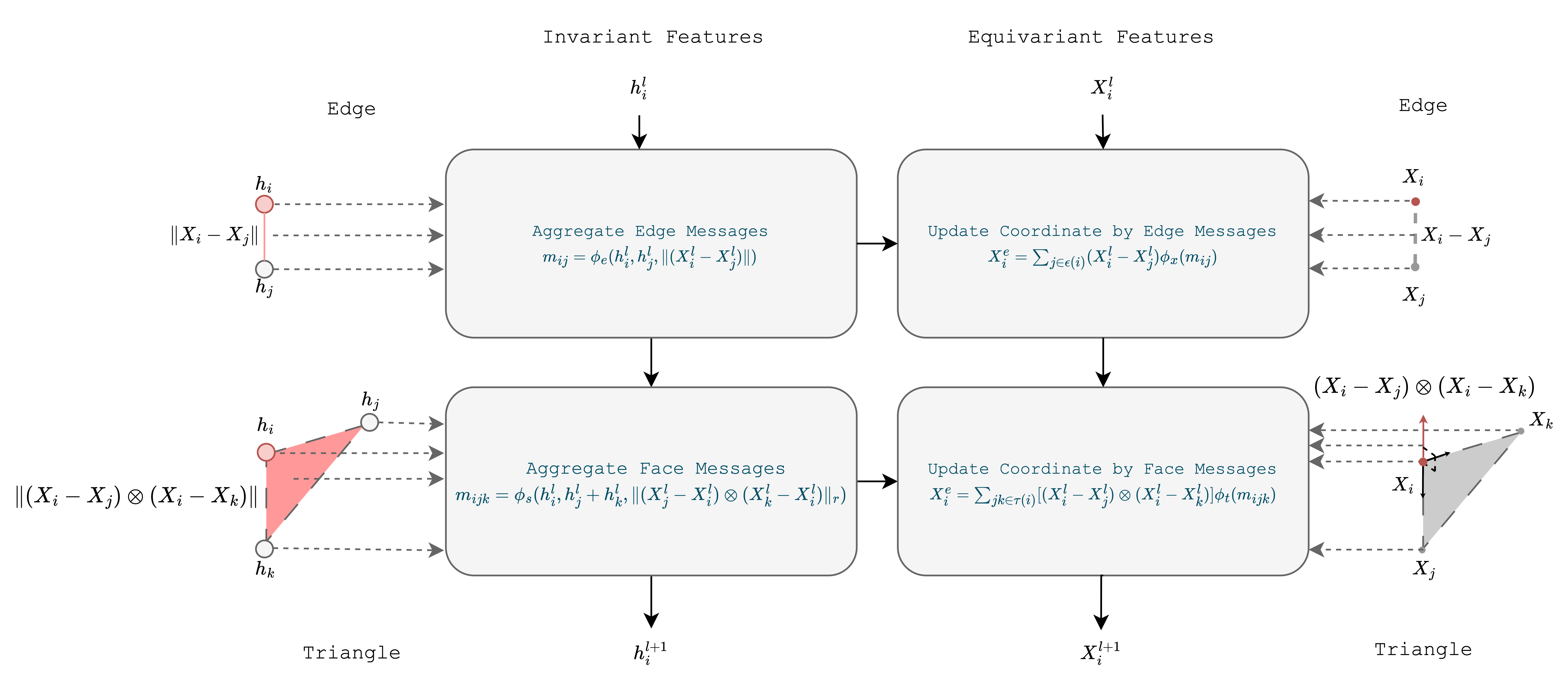
Refer to caption — Figure 1: EMNN Layer - Multi-channels version: On the left-hand side, invariant quantities, such as node’s features, distances between two coordinates, and triangle surface areas, are used to update edge and face messages, denoted as $m_{ij}$ and $m_{ijk}$ , respectively. Subsequently, on the right-hand side, these messages are combined with equivariant quantities, such as node’s coordinates, relative positions between two coordinates, and the triangle surface normal vector, to update the node coordinates.

The key to our extension of EGNN is using normal vectors as quantities that are equivariant to translation and rotation, and triangle surface areas and quantities that are invariant. The way these quantities are integrated into our update equation is analogous to the way distance and relative vectors are integrated in EGNN updates (see Figure 1).

Considering a triangle face ( $i$ , $j$ , $k$ ), we define a surface-aware message from this face to node $i$ as:

m_{ijk}=\phi_{s}\bigg{(}h_{i}^{l},h_{j}^{l}+h_{k}^{l},{\lvert\lvert(x_{j}^{l}-x_{i}^{l})\times(x_{k}^{l}-x_{i}^{l})\rvert\rvert}\bigg{)},

(5)

where $\phi_{s}$ is an MLP. Here, (twice) the surface’s area and the sum of its two adjacent vertices $j$ and $k$ are used to create invariant messages. In particular, this scalar is invariant to rotation, translations, and swapping of nodes $j,k$ . The use of summation as an operation that is invariant to permutation is for simplicity.

Next, the invariant feature for node $i$ is created by aggregating all such messages from neighbouring faces $\tau(i)=\{(j,k)|(i,j,k)\in\mathcal{F}\}$ , and neighbouring edges $\epsilon(i)=\{j|(i,j)\in\mathcal{E}\}$ :

\displaystyle h_{i}^{l+1}

\displaystyle=\phi_{h}\left(h_{i}^{l},\sum_{j\in\epsilon(i)}m_{ij},\sum_{(j,k)\in\tau(i)}m_{ijk}\right).

(6)

Here, the edge message $m_{ij}$ is the same as EGNN equation 2.

The equivariant feature $x_{i}^{l+1}$ is calculated similarly to EGNN update equation 4, with the difference that the normal to neighbouring faces is used as an equivariant vector in the update. This vector is scaled by the invariant factor based on $m_{ijk}$ :

x_{i}^{l+1}=x_{i}^{l}+\sum_{j\in\epsilon(i)}(x_{i}^{l}-x_{j}^{l})\phi_{x}(m_{ij})\\ +\sum_{j,k\in\tau(i)}\left((x^{l}_{j}-x_{i}^{l})\times(x_{k}^{l}-x_{i}^{l})\right)\phi_{t}(m_{ijk}).

(7)

4.1 Multiple Vector Channels

Inspired by Levy et al. (2023), which improves EGNN using multiple vector channels, we also consider a variation of the updates above in which the vector features $x_{i}\in\mathbb{R}^{3}$ are replaced by feature matrices $X_{i}\in\mathbb{R}^{3\times c}$ , where $c$ is the number of vector channels. For $A,B\in\mathbb{R}^{3\times c}$ , let $A\otimes B$ denote the cross product of the corresponding rows – that is $(A\otimes B)_{i,:}=A_{i,:}\times B_{i,:}$ . Moreover, let $\|A\|_{r}$ denote the vector containing row norms of $A$ . Then the generalization of equation 5 to multiple channels is given by

\displaystyle m_{ijk}=\phi_{s}\bigg{(}h_{i}^{l},h_{j}^{l}+h_{k}^{l},{\lvert\lvert(X_{j}^{l}-X_{i}^{l})\otimes(X_{k}^{l}-X_{i}^{l})\rvert\rvert_{r}}\bigg{)}.

(8)

Similarly, equation 7 becomes

X_{i}^{l+1}=X_{i}^{l}+\sum_{j\in\epsilon(i)}(X_{i}^{l}-X_{j}^{l})\phi_{x}(m_{ij})\\ +\sum_{j,k\in\tau(i)}\left((X^{l}_{j}-X_{i}^{l})\otimes(X_{k}^{l}-X_{i}^{l})\right)\phi_{t}(m_{ijk}),

(9)

where, $\phi_{x}$ and $\phi_{t}$ produce invariant $c\times c$ channel mixing matrices as their output. This means rather than simply scaling different equivariant vector features with their corresponding invariant coefficients; we create a linear combination using mixing matrices.

In our experiments, each vertex $p$ in the mesh is augmented with invariant features, such as the average area $a_{p}\in\mathbb{R}$ collected from its adjacent faces; see equation 1. Additionally, in some specific datasets, the other works on mesh leverage heat kernel signatures (HKS) (Sun et al., 2009) as initial features for their networks. In those cases, our work also follows their settings for fair comparisons and reports it in section 5. We use vertex coordinates $x_{p}\in\mathbb{R}^{3}$ and the normal vector $n_{p}\in\mathbb{R}^{3}$ of equation 1 as vector features.

Table 2: Means and standard deviations of our model performance on the FAUST dataset, compared to other equivariant baselines. The training and evaluation are carried out on 5 random seeds without data augmentation.

Model	Initial Features	Accuracy (%)
Model	Initial Features	Train	Test	Gauge	Rot-Tr-Ref-Scale	Perm
GEM-CNN (de Haan et al., 2021)	XYZ	$99.42(0.15)$	$97.92(0.30)$	$96.90(0.25)$	$2.14(1.49)$	$97.92(0.30)$
	GET	$99.42(0.15)$	$98.03(0.17)$	$97.15(0.39)$	$1.47(1.60)$	$98.03(0.17)$
	RELTAN $[0.7]$	$99.69(0.05)$	$98.62(0.06)$	$98.04(0.12)$	$98.62(0.06)$	$98.62(0.06)$
	RELTAN $[0.5,0.7]$	$99.70(0.09)$	$98.64(0.22)$	$97.99(0.18)$	$98.64(0.22)$	$98.64(0.22)$
EMAN (Basu et al., 2022)	XYZ	$99.62(0.09)$	$98.46(0.15)$	$97.26(0.34)$	$0.02(0.00)$	$98.46(0.15)$
	GET	$99.60(0.08)$	$98.43(0.17)$	$97.32(0.46)$	$0.02(0.00)$	$98.43(0.17)$
	RELTAN $[0.7]$	$99.27(1.01)$	$98.13(1.19)$	$97.44(1.26)$	$98.13(1.19)$	$98.13(1.19)$
	$\operatorname{RELTAN}[0.5,0.7]$	$99.68(0.00)$	$98.66(0.07)$	$98.41(0.25)$	$98.66(0.07)$	$98.66(0.07)$
EGNN (baseline)	XYZ	$99.70(0.02)$	$99.50(0.02)$	$99.50(0.02)$	$99.50(0.02)$	$99.50(0.02)$
EGNN + MC (baseline)	XYZ + Normal	$99.80(0.02)$	$99.76(0.01)$	$99.76(0.01)$	$99.76(0.01)$	$99.76(0.01)$
EGNN + MC +Hier (baseline)	XYZ + Normal	$99.94(0.01)$	$99.93(0.01)$	$99.93(0.01)$	$99.93(0.01)$	$99.93(0.01)$
EMNN (ours)	XYZ	$\mathbf{100.00}(0.00)$	$\mathbf{100.00}(0.00)$	$\mathbf{100.00}(0.00)$	$\mathbf{100.00}(0.00)$	$\mathbf{100.00}(0.00)$
EMNN (ours) + MC	XYZ + Normal	$\mathbf{100.00}(0.00)$	$\mathbf{100.00}(0.00)$	$\mathbf{100.00}(0.00)$	$\mathbf{100.00}(0.00)$	$\mathbf{100.00}(0.00)$
EMNN (ours) + MC + Hier	XYZ + Normal	$\mathbf{100.00}(0.00)$	$\mathbf{100.00}(0.00)$	$\mathbf{100.00}(0.00)$	$\mathbf{100.00}(0.00)$	$\mathbf{100.00}(0.00)$

Table 3: Means and standard deviations of our model performance on the TOSCA dataset, compared to other equivariant baselines. The training and evaluation are carried out on 5 random seeds without data augmentation.

Model	Initial Features	Accuracy (%)
Model	Initial Features	Train	Test	Gauge	Rot-Tr-Ref-Scale
GEM-CNN (de Haan et al., 2021)	XYZ	$97.78(2.41)$	$82.35(5.88)$	$82.35(5.88)$	$12.94(2.63)$
	GET	$90.79(2.84)$	$82.35(9.30)$	$82.35(9.30)$	$17.65(7.20)$
	RELTAN[0.7]	$93.97(4.26)$	$91.76(6.71)$	$91.76(6.71)$	$91.76(6.71)$
	RELTAN[0.5, 0.7]	$90.16(8.43)$	$89.41(14.65)$	$89.41(14.65)$	$89.41(14.65)$
EMAN (Basu et al., 2022)	XYZ	$47.30(4.55)$	$42.35(20.55)$	$44.71(18.88)$	$12.94(2.63)$
	GET	$44.13(7.39)$	$42.35(11.31)$	$41.18(9.30)$	$10.59(2.63)$
	RELTAN[0.7]	$92.70(4.14)$	$94.12(4.16)$	$94.12(4.16)$	$94.12(4.16)$
	RELTAN[0.5, 0.7]	$97.46(4.14)$	$98.82(2.63)$	$98.82(2.63)$	$98.82(2.63)$
EGNN (baseline)	XYZ	$96.82(0.11)$	$95.23(0.11)$	$95.23(0.11)$	$95.23(0.11)$
EGNN + MC (baseline)	XYZ + Normal	$\mathbf{100.00}(0.00)$	$\mathbf{100.00}(0.00)$	$\mathbf{100.00}(0.00)$	$\mathbf{100.00}(0.00)$
EGNN + MC + Hier (baseline)	XYZ + Normal	$\mathbf{100.00}(0.00)$	$\mathbf{100.00}(0.00)$	$\mathbf{100.00}(0.00)$	$\mathbf{100.00}(0.00)$
EMNN (ours)	XYZ	$\mathbf{100.00}(0.00)$	$\mathbf{100.00}(0.00)$	$\mathbf{100.00}(0.00)$	$\mathbf{100.00}(0.00)$
EMNN + MC (ours)	XYZ + Normal	$\mathbf{100.00}(0.00)$	$\mathbf{100.00}(0.00)$	$\mathbf{100.00}(0.00)$	$\mathbf{100.00}(0.00)$
EMNN + MC + Hier (ours)	XYZ + Normal	$\mathbf{100.00}(0.00)$	$\mathbf{100.00}(0.00)$	$\mathbf{100.00}(0.00)$	$\mathbf{100.00}(0.00)$

Table 4: Run-time and memory required in 1 epoch of training with batch size equal to 1.

Model	FAUST		TOSCA
Model	Runtime	Memory	Runtime	Memory
GEM-CNN (de Haan et al., 2021)	21s	2.2GB	60s	4.3GB
EMAN (Basu et al., 2022)	53s	2.2GB	120s	6.6GB
EGNN (baseline)	1s	2.1GB	2s	2.7GB
EGNN + MC (baseline)	1.5s	2.1GB	3s	2.7GB
EGNN + MC + Hier (baseline)	2s	2.2GB	4s	2.8GB
EMNN (ours)	3s	2.1GB	7s	3.6GB
EMNN + MC (ours)	4s	2.1GB	11s	3.9GB
EMNN + MC + Hier (ours)	5s	2.2GB	12s	4.0GB

4.2 Analysis of Equivariance

This section discusses the equivariance and invariance properties of our model to the group E(n) of translations, rotations, and reflections. The equivariance of E(n)-EGNN is proved in Satorras et al. (2021), so we only analyze the effect of our extensions. A more formal complete proof of E(3) equivariance and the detail description about complexity of our approach are included in the appendix A.

We can think of the action a euclidean transformation $g\in E(3)$ as acting on a vector $x\in{\mathbb{R}}^{3}$ with a map $x\mapsto Qx+t$ , where $Q\in{\mathbb{R}}^{3\times 3}$ is an orthogonal matrix representing a rotation and/or reflection (with a determinant of 1 or $-1$ ), and $t\in{\mathbb{R}}^{3}$ is a translation vector. A property of the cross product is that if $Q$ is an orthogonal matrix, then for any vectors $u,v\in{\mathbb{R}}^{3}$ , it holds that $Qu\times Qv=\det(Q)Q(u\times v)$ . Another property of the cross product is that $u\times v=-(v\times u)$ . From these two properties, we can see that equation 5 is invariant to any application of an element $g\in$ E(3) and any permutation of $j$ and $k$ . Consequently, equation 6 is also invariant. If we apply a reflection $Q$ where $\det(Q)=-1$ , then naively, the vector update in equation 7 would not be equivariant, as it would reverse the sign of the contribution from the cross product term. However, following the convention that the normal vector of a surface faces outwards, we define the order of $j$ and $k$ so that the cross product $(x_{j}-x_{i})\times(x_{k}-x_{i})$ always faces outwards. By swapping our choice of $j$ and $k$ , we remain equivariant to reflections, and thus all elements of E(3).

4.3 Hierarchical Interactions

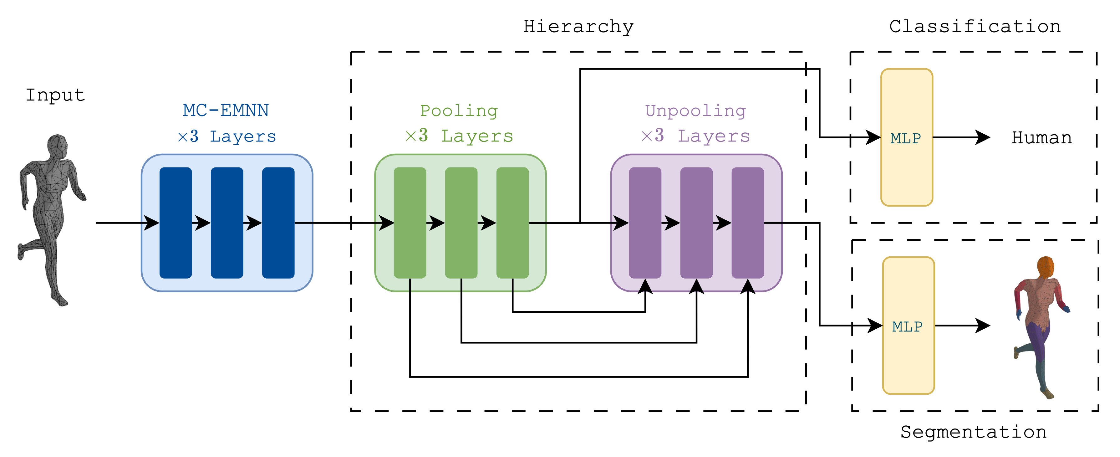
To facilitate long-range communications between nodes, after extracting information using MC-EMNN layers, we employ a hierarchical structure that pools and unpools feature at different resolutions. Our approach is inspired by the hierarchical structure interaction of PointNet++ (Qi et al., 2017a) which includes two main components - pooling and unpooling.

The pooling block (in equation 10) selects a subset of centroid vertices by the Farthest Point Sampling (FPS) algorithm and pools the features from the neighbours of those chosen vertices. The neighbourhood of each vertex $\mathcal{N}(i)$ is defined using a ball of radius $r$ around that vertex. After the pooling process, the selected vertices and their corresponding features serve as inputs for the next layer. The superscript $l$ and the $\phi$ in this section refers to the level of the hierarchy and the MLP, respectively:

\displaystyle h_{i}^{l+1}=\max_{j\in\mathcal{N}(i^{l+1})}(\phi_{P}(h_{j}^{l}))\quad\text{where}\quad i^{l+1}\in\text{FPS}(i^{l})

(10)

In unpooling layers(in equation 11), we calculate a distance-weighted average of features from the higher level in the hierarchy $l$ , and then concatenate this average with the original features of each vertex $h_{i}^{l-1}$ . These original features are extracted from the pooling layer that have the same level in the hierarchy with the considered unpooling layer, visualized in the hierarchy block of figure 2. Here, $\text{KNN}(i^{l-1},i^{l})$ means that for each vertex in level $l-1$ , we find its K nearest neighbours in level $l$ .

\displaystyle h_{i}^{l-1}=\phi_{U}\bigg{(}[\frac{\sum_{j\in\text{KNN}(i^{l-1},i^{l})}\frac{1}{\|x_{ij}\|_{2}}h_{j}}{\sum_{j\in\text{KNN}(i^{l-1},i^{l})}\frac{1}{\|x_{ij}\|_{2}}},h_{i}^{l-1}]\bigg{)}.

(11)

5 Experiments

In this section, we evaluate our models using two types of settings: one for evaluating equivariant models and another for non-equivariant models. Specifically, we have two models EGNN and EMNN with 3 different versions including the original version (EGNN and EMNN), the multiple vector channels version (EGNN + MC and EMNN + MC), and the multiple vector channels version with hierarchical interactions (EGNN + MC + Hier and EMNN + MC + Hier). The evaluations for equivariant models further include tests of robustness to gauge transformations and euclidean transformations. Each setting covers both node-level and graph-level classification. In terms of input features, we maintain the same approach of previous works for a fair comparison. In particular, we use vertex coordinates and normal vectors in the equivariance-evaluation datasets following GEM-CNN (de Haan et al., 2021) and EMAN (Basu et al., 2022), while in other datasets, we additionally pre-compute HKS (Sun et al., 2009) following recent pipelines such as Sharp et al. (2022), Dong et al. (2023a), and Dong et al. (2023b). All experiments in this section are conducted using 1 GPU Nvidia Quadro RTX 5000.

To further achieve scale invariance when comparing to other scale invariant methods, we normalize the initial positions and normal vectors of each vertex. Since our model is designed to be equivariant with E(3) transformations and invariant to scaling, we use no data augmentations when training our EMNN.

5.1 Equivariant Benchmarks

Dataset Description

Datasets used to evaluate equivariant models comprise TOSCA (Bronstein et al., 2008) and FAUST (Bogo et al., 2014):

•

TOSCA is a 9-class mesh dataset of cats, men, women, centaurs, etc with varying nodes and edges in each mesh. This dataset has 80 instances, where 63 meshes are used for training and 17 meshes are used for evaluation. The main task of this dataset is to classify input mesh with correct labels.
•

FAUST includes 100 instances of 3-dimensional human meshes with 6890 vertices each. In each mesh, the vertices are labeled based on body part. This is a segmentation task where the model needs to predict the labels for all vertices in the mesh.

Evaluation

We evaluate EMNN against three other equivariant methods: EMAN (Basu et al., 2022), GEM-CNN (de Haan et al., 2021), and EGNN (Satorras et al., 2021). For EGNN and EMAN, we separate out the contributions of the multi-channel and hierarchical components of the architecture. Following the evaluation procedures of EMAN, we compare across different initial features: coordinates, gauge-equivariant features (GET), relative tangential features (RELTAN), and normal vectors. We also compare robustness to gauge transformations and euclidean transformations.

Results

As observed from table 2 and table 3, EMNN consistently outperforms other equivariant models in both datasets. Furthermore, our method also processes the data with faster run-time and lower memory required, measured in table 4.

5.2 Non-equivariant Benchmarks

Dataset Description

We test the performance of our model on SHREC and Human Body Segmentation:

•

SHREC-11 (Lian et al., 2011) is a classification dataset that contains 30 different classes, each with 20 instances. There are two different train-test split settings commonly used for evaluation: 10-10 and 16-4 per-class train-test split.
•

Human Body Segmentation has 370 meshes for training and 18 meshes for testing, which were collected from Adobe Fuse (Adobe, 2016), FAUST (Bogo et al., 2014), MIT (Vlasic et al., 2008), SCAPE (Klokov and Lempitsky, 2017), and SHREC07 (Giorgi et al., 2007). Thereafter all the meshes are labeled into 8 parts by (Giorgi et al., 2007).

Results

Our method is compared against alternatives in table 5. EMNN achieved SOTA on 16-4 split settings, while placed second in the 10-10 settings. table 6 reports our results for Human Body Segmentation dataset.

Table 5: The best results of EMNN on the SHREC dataset, the run-time, and memory are measured when training for 1 epoch and with batch size equal to 1.

Method	Runtime	Memory	Split-16	Split-10
GWCNN (Ezuz et al., 2017)	—	—	$96.6\%$	$90.3\%$	\rdelim}517.5mm[ Invariant Methods ]
MeshCNN (Hanocka et al., 2019)	50s	1.2GB	$98.6\%$	$91.0\%$
PD-MeshNet (Milano et al., 2020)	—	—	$99.7\%$	$99.1\%$
MeshWalker(Lahav and Tal, 2020)	—	—	$98.6\%$	$97.1\%$
HodgeNet (Smirnov and Solomon, 2021)	—	—	$99.2\%$	$94.7\%$
SubdivNet (Hu et al., 2022)	25s	0.9GB	$99.9\%$	$99.5\%$	\rdelim}417.5mm[ Non-invariant Methods ]
DiffusionNet(Sharp et al., 2022)	16s	1.0GB	—	$99.5\%$
Laplacian2Mesh (Dong et al., 2023a)	30s	2.8GB	$\mathbf{100}\%$	$\mathbf{100}\%$
Mesh-MLP (Dong et al., 2023b)	—	—	$\mathbf{100}\%$	$99.7\%$
EGNN (baseline)	11s	0.8GB	$99.1\%$	$96.3\%$	\rdelim}317.5mm[ EGNN ]
EGNN + MC (baseline)	11s	0.8GB	$100\%$	$99.3\%$
EGNN + MC + Hier (baseline)	11s	0.8GB	$100\%$	$99.6\%$
EMNN (ours)	24s	1.1GB	100%	$97.3\%$	\rdelim}317.5mm[ EMNN ]
EMNN + MC (ours)	25s	1.1GB	100%	99.7%
EMNN + MC + Hier (ours)	26s	1.2GB	100%	100%%

Table 6: The best results of EMNN on the Human Body Segmentation, the run-time, and memory are measured when training for 1 epoch and with batch size equal to 1.

Method	Input	Runtime	Memory	Accuracy
PointNet (Qi et al., 2017b)	point cloud	12s	1.2GB	$74.7\%$	\rdelim}117.5mm[ Point cloud Methods ]
PointNet++(Qi et al., 2017a)	point cloud	10s	0.9GB	$82.3\%$
MeshCNN (Hanocka et al., 2019)	mesh	137s	1.4GB	$85.4\%$	\rdelim}317.5mm[ Invariant Methods ]
PD-MeshNet (Milano et al., 2020)	mesh	—	—	$85.6\%$
HodgeNet (Smirnov and Solomon, 2021)	mesh	—	—	$85.0\%$
SubdivNet (Hu et al., 2022)	mesh	100s	1.3GB	$\textbf{91.7}\%$	\rdelim}417.5mm[ Non-invariant Methods ]
DiffusionNet (Sharp et al., 2022)	mesh	16s	2.0GB	$90.3\%$
Laplacian2Mesh (Dong et al., 2023a)	mesh	70s	4.8GB	$88.6\%$
Mesh-MLP (Dong et al., 2023b)	mesh	—	—	$88.8\%$
EGNN (baseline)	graph	10s	0.8GB	$80.6\%$	\rdelim}317.5mm[ EGNN ]
EGNN+MC (baseline)	graph	11s	0.8GB	$82.7\%$
EGNN+MC+Hier (baseline)	graph	16s	0.9GB	$87.2\%$
EMNN (ours)	mesh	18s	0.9GB	$81.0\%$	\rdelim}317.5mm[ EMNN ]
EMNN+MC (ours)	mesh	20s	0.9GB	$83.5\%$
EMNN+MC+Hier (ours)	mesh	26s	1.0GB	88.7%

5.3 Ablation Study

We conducted an ablation study on the number of EMNN layers, depth of the hierarchy, and the number of channels on the Human Body Segmentation dataset. Results in table 7 show that EMNN achieves its best performance with 3 layers of EMNN, 3-level hierarchical structure, and 2-channel vectors. We used these hyper-parameters for all other datasets.

5.4 Software

Our source code in PyTorch (Paszke et al., 2019) is at https://github.com/HySonLab/EquiMesh.

Table 7: Ablation studies on Layers, Hierarchy, Channels on the Human Body Segmentation.

Layers	Accuracy	Hierarchy	Accuracy	Channels	Accuracy
2	87.5	2	88.2	2	88.7
3	88.7	3	88.7	4	86.3
4	88.0	4	87.6	8	88.2

6 Conclusion

In this work, we introduce the Equivariant Mesh Neural Network (EMNN), a simple yet efficient model that is equivariant to Euclidean transformations. Our motivation for introducing yet another equivariant network for mesh data is the observation that EGNN, a geometric graph neural network, performs surprisingly well on meshes. This can be seen in all our experiments. In particular, the addition of multiple channels and hierarchy further improves EGNN making it competitive with architectures specialized to mesh data.

We observe that the main property of meshes ignored by EGNN updates is the use of information contained in their triangular faces. We capture this information using a cross product, which creates new invariants based on area and new equivariant quantities based on normals in successive layers, augmenting the invariant and equivariant features used by EGNN. The result is a simple addition to EGNN, which result in further improvement in its performance, as shown in our experiments. As a final step, we improve EMNN with multiple vector channels and pooling/unpooling operations to handle long-range interactions, empirically showing the benefit of each of these components.

In practical terms, our EMNN surpasses more complex equivariant architectures such as GEM-CNN (de Haan et al., 2021) and EMAN (Basu et al., 2022) in accuracy, while remaining 4-10x faster. Furthermore, our model produces competitive results in terms of runtime, memory, and accuracy when compared with non-equivariant models.

7 Acknowledgements

SR and DL are partly supported by CIFAR and NSERC.

References

Adobe (2016) Adobe (2016). Adobe fuse 3d characters. https://www.mixamo.com.
Anderson et al. (2019) Anderson, B., Hy, T.-S., and Kondor, R. (2019). Cormorant: covariant molecular neural networks. Curran Associates Inc., Red Hook, NY, USA.
Basu et al. (2022) Basu, S., Gallego-Posada, J., Viganò, F., Rowbottom, J., and Cohen, T. (2022). Equivariant Mesh Attention Networks. Transactions on Machine Learning Research.
Bogo et al. (2014) Bogo, F., Romero, J., Loper, M., and Black, M. J. (2014). Faust: Dataset and evaluation for 3d mesh registration. In 2014 IEEE Conference on Computer Vision and Pattern Recognition, pages 3794–3801.
Boscaini et al. (2016) Boscaini, D., Masci, J., Rodolà, E., and Bronstein, M. (2016). Learning shape correspondence with anisotropic convolutional neural networks. In D. Lee, M. Sugiyama, U. Luxburg, I. Guyon, and R. Garnett, editors, Advances in Neural Information Processing Systems, volume 29. Curran Associates, Inc.
Brandstetter et al. (2022) Brandstetter, J., Hesselink, R., van der Pol, E., Bekkers, E. J., and Welling, M. (2022). Geometric and physical quantities improve e(3) equivariant message passing. In International Conference on Learning Representations.
Bronstein et al. (2008) Bronstein, A. M., Bronstein, M. M., and Kimmel, R. (2008). Numerical Geometry of Non-Rigid Shapes. Springer Science & Business Media.
Cai et al. (2023) Cai, C., Hy, T. S., Yu, R., and Wang, Y. (2023). On the connection between MPNN and graph transformer. In A. Krause, E. Brunskill, K. Cho, B. Engelhardt, S. Sabato, and J. Scarlett, editors, Proceedings of the 40th International Conference on Machine Learning, volume 202 of Proceedings of Machine Learning Research, pages 3408–3430. PMLR.
Cohen et al. (2019) Cohen, T., Weiler, M., Kicanaoglu, B., and Welling, M. (2019). Gauge equivariant convolutional networks and the icosahedral CNN. In K. Chaudhuri and R. Salakhutdinov, editors, Proceedings of the 36th International Conference on Machine Learning, volume 97 of Proceedings of Machine Learning Research, pages 1321–1330. PMLR.
Cohen et al. (2018) Cohen, T. S., Geiger, M., Köhler, J., and Welling, M. (2018). Spherical CNNs. In International Conference on Learning Representations.
de Haan et al. (2021) de Haan, P., Weiler, M., Cohen, T., and Welling, M. (2021). Gauge equivariant mesh cnns: Anisotropic convolutions on geometric graphs. In International Conference on Learning Representations.
Dong et al. (2023a) Dong, Q., Wang, Z., Li, M., Gao, J., Chen, S., Shu, Z., Xin, S., Tu, C., and Wang, W. (2023a). Laplacian2mesh: Laplacian-based mesh understanding. IEEE Transactions on Visualization and Computer Graphics.
Dong et al. (2023b) Dong, Q., Xu, R., Gong, X., Wang, Z., Chen, S., Xin, S., and Tu, C. (2023b). Mesh-mlp: An all-mlp architecture for mesh classification and semantic segmentation.
Dwivedi et al. (2022) Dwivedi, V. P., Rampášek, L., Galkin, M., Parviz, A., Wolf, G., Luu, A. T., and Beaini, D. (2022). Long range graph benchmark. In S. Koyejo, S. Mohamed, A. Agarwal, D. Belgrave, K. Cho, and A. Oh, editors, Advances in Neural Information Processing Systems, volume 35, pages 22326–22340. Curran Associates, Inc.
Eijkelboom et al. (2023) Eijkelboom, F., Hesselink, R., and Bekkers, E. J. (2023). E $(n)$ equivariant message passing simplicial networks. In A. Krause, E. Brunskill, K. Cho, B. Engelhardt, S. Sabato, and J. Scarlett, editors, Proceedings of the 40th International Conference on Machine Learning, volume 202 of Proceedings of Machine Learning Research, pages 9071–9081. PMLR.
Ezuz et al. (2017) Ezuz, D., Solomon, J., Kim, V. G., and Ben-Chen, M. (2017). Gwcnn: A metric alignment layer for deep shape analysis. Comput. Graph. Forum, 36(5), 49–57.
Feng et al. (2019) Feng, Y., Feng, Y., You, H., Zhao, X., and Gao, Y. (2019). Meshnet: Mesh neural network for 3d shape representation. In Proceedings of the AAAI Conference on Artificial Intelligence, volume 33, pages 8279–8286.
Gao et al. (2019) Gao, L., Yang, J., Wu, T., Yuan, Y.-J., Fu, H., Lai, Y.-K., and Zhang, H. (2019). Sdm-net: Deep generative network for structured deformable mesh. ACM Trans. Graph., 38(6).
Gasteiger et al. (2021) Gasteiger, J., Yeshwanth, C., and Günnemann, S. (2021). Directional message passing on molecular graphs via synthetic coordinates. In M. Ranzato, A. Beygelzimer, Y. Dauphin, P. Liang, and J. W. Vaughan, editors, Advances in Neural Information Processing Systems, volume 34, pages 15421–15433. Curran Associates, Inc.
Gilmer et al. (2017) Gilmer, J., Schoenholz, S. S., Riley, P. F., Vinyals, O., and Dahl, G. E. (2017). Neural message passing for quantum chemistry. In International conference on machine learning, pages 1263–1272. PMLR.
Giorgi et al. (2007) Giorgi, D., Biasotti, S., and Paraboschi, L. (2007). Shape retrieval contest 2007: Watertight models track. SHREC competition, 8(7), 7.
Gong et al. (2019) Gong, S., Chen, L., Bronstein, M., and Zafeiriou, S. (2019). Spiralnet++: A fast and highly efficient mesh convolution operator. In Proceedings of the IEEE International Conference on Computer Vision Workshops, pages 0–0.
Hanocka et al. (2019) Hanocka, R., Hertz, A., Fish, N., Giryes, R., Fleishman, S., and Cohen-Or, D. (2019). Meshcnn: A network with an edge. ACM Transactions on Graphics (TOG), 38(4), 90:1–90:12.
Hu et al. (2022) Hu, S., Liu, Z., Guo, M., Cai, J., Huang, J., Mu, T., and Martin, R. R. (2022). Subdivision-based mesh convolution networks. ACM Trans. Graph., 41(3), 25:1–25:16.
Huang et al. (2019) Huang, J., Zhang, H., Yi, L., Funkhouser, T., Nießner, M., and Guibas, L. J. (2019). Texturenet: Consistent local parametrizations for learning from high-resolution signals on meshes. In Proceedings of the IEEE Conference on Computer Vision and Pattern Recognition, pages 4440–4449.
Hy et al. (2018) Hy, T. S., Trivedi, S., Pan, H., Anderson, B. M., , and Kondor, R. (2018). Predicting molecular properties with covariant compositional networks. The Journal of Chemical Physics, 148.
Hy et al. (2019) Hy, T. S., Trivedi, S., Pan, H., Anderson, B. M., and Kondor, R. (2019). Covariant compositional networks for learning graphs. In Proc. International Workshop on Mining and Learning with Graphs (MLG).
Klokov and Lempitsky (2017) Klokov, R. and Lempitsky, V. S. (2017). Escape from cells: Deep kd-networks for the recognition of 3d point cloud models. 2017 IEEE International Conference on Computer Vision (ICCV), pages 863–872.
Lahav and Tal (2020) Lahav, A. and Tal, A. (2020). Meshwalker: Deep mesh understanding by random walks. ACM Trans. Graph., 39(6).
Levy et al. (2023) Levy, D., Kaba, S.-O., Gonzales, C., Miret, S., and Ravanbakhsh, S. (2023). Using multiple vector channels improves e (n)-equivariant graph neural networks. arXiv preprint arXiv:2309.03139.
Lian et al. (2011) Lian, Z., Godil, A., Bustos, B., Daoudi, M., Hermans, J., Kawamura, S., Kurita, Y., Lavoué, G., Nguyen, H., Ohbuchi, R., Ohkita, Y., Ohishi, Y., Porikli, F., Reuter, M., Sipiran, I., Smeets, D., Suetens, P., Tabia, H., and Vandermeulen, D. (2011). Shrec ’11 track: Shape retrieval on non-rigid 3d watertight meshes. pages 79–88.
Lim et al. (2018) Lim, I., Dielen, A., Campen, M., and Kobbelt, L. P. (2018). A simple approach to intrinsic correspondence learning on unstructured 3d meshes. ArXiv, abs/1809.06664.
Luebke et al. (2002) Luebke, D., Watson, B., Cohen, J. D., Reddy, M., and Varshney, A. (2002). Level of Detail for 3D Graphics. Elsevier Science Inc., USA.
Masci et al. (2015) Masci, J., Boscaini, D., Bronstein, M. M., and Vandergheynst, P. (2015). Geodesic convolutional neural networks on riemannian manifolds. In 2015 IEEE International Conference on Computer Vision Workshop (ICCVW), pages 832–840.
Milano et al. (2020) Milano, F., Loquercio, A., Rosinol, A., Scaramuzza, D., and Carlone, L. (2020). Primal-dual mesh convolutional neural networks. In Conference on Neural Information Processing Systems (NeurIPS).
Monti et al. (2017) Monti, F., Boscaini, D., Masci, J., Rodolà, E., Svoboda, J., and Bronstein, M. (2017). Geometric deep learning on graphs and manifolds using mixture model cnns. pages 5425–5434.
Ngo et al. (2023) Ngo, N. K., Hy, T. S., and Kondor, R. (2023). Multiresolution graph transformers and wavelet positional encoding for learning long-range and hierarchical structures. The Journal of Chemical Physics, 159(3), 034109.
Paszke et al. (2019) Paszke, A., Gross, S., Massa, F., Lerer, A., Bradbury, J., Chanan, G., Killeen, T., Lin, Z., Gimelshein, N., Antiga, L., Desmaison, A., Köpf, A., Yang, E., DeVito, Z., Raison, M., Tejani, A., Chilamkurthy, S., Steiner, B., Fang, L., Bai, J., and Chintala, S. (2019). PyTorch: an imperative style, high-performance deep learning library. Curran Associates Inc., Red Hook, NY, USA.
Qi et al. (2017a) Qi, C. R., Yi, L., Su, H., and Guibas, L. J. (2017a). Pointnet++: Deep hierarchical feature learning on point sets in a metric space. In I. Guyon, U. V. Luxburg, S. Bengio, H. Wallach, R. Fergus, S. Vishwanathan, and R. Garnett, editors, Advances in Neural Information Processing Systems, volume 30. Curran Associates, Inc.
Qi et al. (2017b) Qi, C. R., Su, H., Mo, K., and Guibas, L. J. (2017b). Pointnet: Deep learning on point sets for 3d classification and segmentation. In Proceedings of the IEEE conference on computer vision and pattern recognition, pages 652–660.
Ranjan et al. (2018) Ranjan, A., Bolkart, T., Sanyal, S., and Black, M. J. (2018). Generating 3d faces using convolutional mesh autoencoders. In V. Ferrari, M. Hebert, C. Sminchisescu, and Y. Weiss, editors, Computer Vision – ECCV 2018, pages 725–741, Cham. Springer International Publishing.
Rogers (1986) Rogers, D. F. (1986). Procedural elements for computer graphics. McGraw-Hill, Inc.
Satorras et al. (2021) Satorras, V. G., Hoogeboom, E., and Welling, M. (2021). E(n) equivariant graph neural networks. In M. Meila and T. Zhang, editors, Proceedings of the 38th International Conference on Machine Learning, volume 139 of Proceedings of Machine Learning Research, pages 9323–9332. PMLR.
Schult et al. (2020) Schult, J., Engelmann, F., Kontogianni, T., and Leibe, B. (2020). Dualconvmesh-net: Joint geodesic and euclidean convolutions on 3d meshes. In 2020 IEEE/CVF Conference on Computer Vision and Pattern Recognition (CVPR), pages 8609–8619.
Schütt et al. (2018) Schütt, K. T., Sauceda, H. E., Kindermans, P.-J., Tkatchenko, A., and Müller, K.-R. (2018). SchNet – A deep learning architecture for molecules and materials. The Journal of Chemical Physics, 148(24), 241722.
Sharp et al. (2022) Sharp, N., Attaiki, S., Crane, K., and Ovsjanikov, M. (2022). Diffusionnet: Discretization agnostic learning on surfaces. ACM Trans. Graph., 41(3).
Smirnov and Solomon (2021) Smirnov, D. and Solomon, J. (2021). Hodgenet: Learning spectral geometry on triangle meshes. ACM Trans. Graph., 40(4).
Sun et al. (2009) Sun, J., Ovsjanikov, M., and Guibas, L. J. (2009). A concise and provably informative multi‐scale signature based on heat diffusion. Computer Graphics Forum, 28.
Tatarchenko et al. (2018) Tatarchenko, M., Park, J., Koltun, V., and Zhou, Q.-Y. (2018). Tangent convolutions for dense prediction in 3d. In Proceedings of the IEEE conference on computer vision and pattern recognition, pages 3887–3896.
Thomas et al. (2018) Thomas, N., Smidt, T., Kearnes, S., Yang, L., Li, L., Kohlhoff, K., and Riley, P. (2018). Tensor field networks: Rotation-and translation-equivariant neural networks for 3d point clouds. arXiv preprint arXiv:1802.08219.
Verma et al. (2018) Verma, N., Boyer, E., and Verbeek, J. (2018). Feastnet: Feature-steered graph convolutions for 3d shape analysis. In Proceedings of the IEEE conference on computer vision and pattern recognition, pages 2598–2606.
Vlasic et al. (2008) Vlasic, D., Baran, I., Matusik, W., and Popović, J. (2008). Articulated mesh animation from multi-view silhouettes. ACM SIGGRAPH 2008 papers.
Weiler et al. (2021) Weiler, M., Forré, P., Verlinde, E., and Welling, M. (2021). Coordinate independent convolutional networks – isometry and gauge equivariant convolutions on riemannian manifolds.

Appendix A Proof of Equivariance

In this section, we show that the update equations of a layer of EMNN is equivariant to the action of $g\in\mathrm{E}(3)$ . An element $g$ can act on a vector $x\in{\mathbb{R}}^{3}$ as $x\mapsto Qx+t$ for translation vector $t\in{\mathbb{R}}^{3}$ and orthogonal matrix $Q\in{\mathbb{R}}^{3\times 3}$ where $Q^{\top}Q=I$ and $\det(Q)\in\{-1,1\}$ . The matrix $Q$ can be considered a representation of an element of the orthogonal group O(3), a subgroup of E(3). If $\det(Q)=1$ , then $Q$ represents a rotation, and if $\det(Q)=-1$ , then it represents a rotoreflection or a reflection.

First, we show that the cross product is equivariant to orthogonal transformations, up to a sign change. Specifically, given vectors $u,v\in{\mathbb{R}}^{3}$ , a group element $g\in\mathrm{O}(3)$ , and the corresponding orthogonal matrix $Q\in{\mathbb{R}}^{3\times 3}$ we want to show that $Q(u\times v)\in\det(Q)(Qu\times Qv)$ where $\det(Q)$ is -1 or 1. We make use of the scalar triple product property: $\forall u,v,w\in{\mathbb{R}}^{3},\hskip 12.0ptw\cdot(u\times v)=\det([w\hskip 6.0ptu\hskip 6.0ptv])$ So for any vector $w$ , we have:

	$\displaystyle w\cdot(Qu\times Qv)$	$\displaystyle=\det([w\hskip 6.0ptQu\hskip 6.0ptQv])$
		$\displaystyle=\det(Q[Q^{\top}w\hskip 6.0ptu\hskip 6.0ptv])$
		$\displaystyle=\det(Q)\det([Q^{\top}w\hskip 6.0ptu\hskip 6.0ptv])$
		$\displaystyle=\det(Q)Q^{\top}w\cdot(u\times v)$
		$\displaystyle=\det(Q)(Q^{\top}w)^{\top}(u\times v)$
		$\displaystyle=\det(Q)w\cdot Q(u\times v)$

where we use the fact that $Q^{T}Q=I$ . Since we can set $w$ to basis vectors $e_{1},e_{2}$ and $e_{3}$ , we can see that $(Qu\times Qv)_{i}=\det(Q)(Q(u\times v))_{i}$ for $i=1,2,3$ , so $(Qu\times Qv)=\det(Q)Q(u\times v)$ .

Next, we can easily see that for any $v\in{\mathbb{R}}^{3}$ and rotation matrix $Q$ , $||Qv||=\sqrt{v^{\top}Q^{\top}Qv}=||v||$ , using $Q^{\top}Q=I$ .

From this, we can see that the messages $m_{ij}$ and $m_{ijk}$ from equations (2) and (5) are invariant, assuming $h^{l}_{i}$ , $h^{l}_{j}$ , and $h^{l}_{k}$ do not depend on $x$ . If the action of $g\in E(3)$ is $x\mapsto Qx+t$ , then in equation (2) we see:

\displaystyle||((Qx_{i}+t)-(Qx_{j}+t))||

\displaystyle=||Q(x_{i}-x_{j})||=||(x_{i}-x_{j})||,

so $m_{ij}$ is invariant to E(3). In equation (5) we see:

	$\displaystyle\|\|((Qx_{j}+t)-(Qx_{i}+t))\times((Qx_{k}+t)-(Qx_{i}+t))\|\|$	$\displaystyle=\|\|Q(x_{j}-x_{i})\times Q(x_{k}-x_{i})\|\|$
		$\displaystyle=\|\|\det(Q)Q((x_{j}-x_{i})\times(x_{k}-x_{i}))\|\|$
		$\displaystyle=\|\|(x_{j}-x_{i})\times(x_{k}-x_{i})\|\|,$

so $m_{ijk}$ is invariant to E(3). Knowing this, we can see that the embedding $h_{i}^{l+1}$ in equation (6)) is invariant to E(3).

Next, we can see that the coordinate update of equation (7) is equivariant to E(3):

	$\displaystyle(Qx_{i}^{l}+t)$	$\displaystyle+\sum_{j\in\epsilon(i)}((Qx_{i}^{l}+t)-(Qx_{j}^{l}+t))\phi_{x}(m_{ij})$
		$\displaystyle+\sum_{j,k\in\tau(i)}\left((Qx^{l}_{j}+t)-(Qx_{i}^{l}+t)\times((Qx_{k}^{l}+t)-(Qx_{i}^{l}+t))\right)\phi_{t}(m_{ijk})$
	$\displaystyle=(Qx_{i}^{l}+t)$	$\displaystyle+\sum_{j\in\epsilon(i)}(Qx_{i}^{l}-Qx_{j}^{l})\phi_{x}(m_{ij})$
		$\displaystyle+\sum_{j,k\in\tau(i)}\left((Qx^{l}_{j}-Qx_{i}^{l})\times((Qx_{k}^{l}-Qx_{i}^{l})\right)\phi_{t}(m_{ijk})$
	$\displaystyle=(Qx_{i}^{l}+t)$	$\displaystyle+\sum_{j\in\epsilon(i)}Q(x_{i}^{l}-x_{j}^{l})\phi_{x}(m_{ij})+\sum_{j,k\in\tau(i)}\left(Q(x^{l}_{j}-x_{i}^{l})\times Q(x_{k}^{l}-x_{i}^{l})\right)\phi_{t}(m_{ijk})$
	$\displaystyle=Qx_{i}^{l}+t$	$\displaystyle+Q\sum_{j\in\epsilon(i)}(x_{i}^{l}-x_{j}^{l})\phi_{x}(m_{ij})+\det(Q)Q\sum_{j,k\in\tau(i)}\left((x^{l}_{j}-x_{i}^{l})\times(x_{k}^{l}-x_{i}^{l})\right)\phi_{t}(m_{ijk})$

	$\displaystyle=Q\left(x_{i}^{l}+\sum_{j\in\epsilon(i)}(x_{i}^{l}-x_{j}^{l})\phi_{x}(m_{ij})+\sum_{j^{\prime},k^{\prime}\in\tau(i)}\left((x^{l}_{j^{\prime}}-x_{i}^{l})\times(x_{k^{\prime}}^{l}-x_{i}^{l})\right)\phi_{t}(m_{ijk})\right)+t$
	$\displaystyle=Q(x_{i}^{l+1})+t$

In the second to last line, we replace $j,k\in\tau(i)$ with $j^{\prime},k^{\prime}\in\tau(i)$ , where $j^{\prime},k^{\prime}=k,j$ if $\det(Q)=-1$ and $j^{\prime},k^{\prime}=j,k$ if $\det(Q)=1$ . We are able to do this because we have defined the order of $\tau(i)$ such that the normal vector $(x_{j}-x_{i})\times(x_{k}-x_{i})$ always faces outwards. Thus, if we reflect our input coordinates, then we would also need to swap the order of $j$ and $k$ . A matrix representing a reflection has $\det(Q)=-1$ , and the cross product has the anticommutative property $u\times v=-(v\times u)$ , so $\det(Q)\sum_{j,k\in\tau(i)}((x_{j}-x_{i})\times(x_{k}-x_{i}))=\sum_{j^{\prime},k^{\prime}\in\tau(i)}((x_{j^{\prime}}-x_{i})\times(x_{k^{\prime}}-x_{i}))$ .

Put together,this shows that when applying a layer of EMNN, $h$ is updated in manner invariant to E(3), and $x$ is updated in a manner equivariant to E(3). This proof can trivially be extended to the multi-channel case by noting that the multi-channel operations in equation (8) and (9) operate separately across each vector channel except for the channel-mixing matrices $\phi_{t}(m_{ijk})$ and $\phi_{x}(m_{ij})$ , which only scale vectors in a way that’s invariant to E(3).

Appendix B Time & Space Complexity of EMNN

In terms of asymptotic computational complexity, our method is identical to EGNN. This is because the number of neighbouring faces of a node is at most the number of its neighbouring nodes, so including face information does not increase the asymptotic complexity.
Time Complexity: EMNN’s time complexity is $\mathcal{O}(M+\max_{i}N(i))$ , where $N(i)$ are the number of neighbours of node $i$ and $M$ is the number of edges. With multi-channel the time complexity is increased to $O((M+\max_{i}N(i))CC^{\prime})$ with $C$ and $C^{\prime}$ are the number of input and output vectors, respectively.
Space Complexity: EMNN’s space complexity is likewise the same as EGNN, of order $\mathcal{O}(Nd+NC)$ where $d$ is the dimension of the embedding of each node.

	$\displaystyle\|\|((Qx_{j}+t)-(Qx_{i}+t))\times((Qx_{k}+t)-(Qx_{i}+t))\|\|$	$\displaystyle=\|\|Q(x_{j}-x_{i})\times Q(x_{k}-x_{i})\|\|$
		$\displaystyle=\|\|\det(Q)Q((x_{j}-x_{i})\times(x_{k}-x_{i}))\|\|$
		$\displaystyle=\|\|(x_{j}-x_{i})\times(x_{k}-x_{i})\|\|,$