Discovering More Effective Tensor Network Structure Search Algorithms
via Large Language Models (LLMs)
Abstract
Tensor network structure search (TN-SS), aiming at searching for suitable tensor network (TN) structures in representing high-dimensional problems, largely promotes the efficacy of TN in various machine learning applications. Nonetheless, finding a satisfactory TN structure using existing algorithms remains challenging. To develop more effective algorithms and avoid the human labor-intensive development process, we explore the knowledge embedded in large language models (LLMs) for the automatic design of TN-SS algorithms. Our approach, dubbed GPTN-SS, leverages an elaborate crafting LLM-based prompting system that operates in an evolutionary-like manner. The experimental results, derived from real-world data, demonstrate that GPTN-SS can effectively leverage the insights gained from existing methods to develop novel TN-SS algorithms that achieve a better balance between exploration and exploitation. These algorithms exhibit superior performance in searching the high-quality TN structures for natural image compression and model parameters compression while also demonstrating generalizability in their performance.
1 Introduction
Tensor networks (TNs) are powerful methods that have proven to be highly beneficial in the fields of computer science and quantum physics (Markov & Shi, 2008; Anandkumar et al., 2014; Orús, 2014; Novikov et al., 2015; Cichocki et al., 2016; Stoudenmire & Schwab, 2016; Cichocki et al., 2017; Orús, 2019; Glasser et al., 2019; Kossaifi et al., 2020; Miller et al., 2021; Richter et al., 2021; Miller et al., 2021; Richter et al., 2021; Haghshenas et al., 2022). Their effectiveness lies in the ability to efficiently analyze and compute high-dimensional problems. However, selecting the optimal TN structure can be a challenging task (Li & Sun, 2020). To confront this, many TN practitioners have put their efforts into addressing the problem of tensor network structure search (TN-SS), where the goal is to search for the optimal TN structure for high-dimensional representation.
There are multiple approaches to solving this problem (Li & Sun, 2020; Nie et al., 2021; Zheng et al., 2023b). Among these methods, treating TN-SS as a discrete optimization problem and solving it using heuristic approaches, including evolutionary algorithms (Li & Sun, 2020), greedy strategies (Hashemizadeh et al., 2020), and local sampling (Li et al., 2022, 2023), has demonstrated superior flexibility. This approach is particularly effective in addressing TN-SS of higher orders and higher TN-ranks. Specifically, the local sampling method leverages the local smoothness priors within the TN-SS landscape, effectively reducing the computational demand for evaluating TN structures to a manageable level. However, due to its local essence, it may stuck in the bad local optima when working with real-world tensors (Li et al., 2023). On the other hand, evolutionary algorithms usually perform better in these situations, but they need a lot of evaluation. To further develop more effective TN-SS algorithms, it is crucial to introduce new heuristics. Traditionally, this process involves a labor-intensive cycle, encompassing literature review, algorithm design, and experimental evaluation. However, one may wonder whether there exists a more effective and automatic way and also be curious about a question: How far will this cycle take us?

The recent work by (Romera-Paredes et al., 2023), which employs a large language model (LLM) for mathematical discoveries, provides a hint. It reveals that LLMs can independently generate innovative solutions to the open math problem known as the cap set, surpassing the best results previously attained by mathematicians after decades of effort. Consequently, this insight sheds light on the preceding question: in certain areas, the experts’ ways of problem-solving may encounter bottlenecks, whereas LLMs can offer breakthroughs. Indeed, with the recent tremendous growth in scale of LLMs and the availability of vast amounts of text data on the internet, LLMs demonstrate surprising emergent capabilities in programming (Haluptzok et al., 2022; Tian et al., 2023), doing math (Noorbakhsh et al., 2021), solving logical problems (Creswell et al., 2022) and many other domains (Boiko et al., 2023; Nori et al., 2023; Blocklove et al., 2023). The knowledge embedded within LLMs enables them to potentially serve as a general-purpose model (Achiam et al., 2023; Bubeck et al., 2023). Motivated by these, this research aims to uncover the embedded knowledge of the LLMs for designing TN-SS algorithms and construct an automated framework for TN-SS algorithm design.
While direct one-shot queries to LLMs often fall short in addressing complex, real-world tasks, a growing body of research is focusing on developing elaborately designed systems to better leverage LLMs’ hidden knowledge (Romera-Paredes et al., 2023; Chen et al., 2023; Cai et al., 2023). In this study, we explore the capacity of LLMs for automatic TN-SS algorithm design. To this end, we have developed an evolutionary-like designing system, in which LLM functions as the main operator. This system is depicted in Figure 1 and is referred to as GPTN-SS.
As shown in Figure 1, GPTN-SS is fundamentally inspired by the human expert’s algorithm design process, encompassing two pivotal phases: knowledge exploitation and exploration. In the knowledge exploitation phase, GPTN-SS utilizes available knowledge in the existing methods for better algorithm design. Specifically, it has two key components: crossover and mutation. Crossover is dedicated to leveraging the combined strengths of various algorithms, encouraging the LLM to build upon and improve over them. Meanwhile, the mutation focuses on making local improvements to the specific components of the algorithms. For instance, the LLM could enhance a given algorithm by focusing on tuning its hyperparameters. In contrast, the other core phase of GPTN-SS, knowledge exploration, aims to explore the diversity of algorithm design methodologies. This phase is inspired by previous work in Quality Diversity (QD) methods (Pugh et al., 2016). Here, we maintain a pool of algorithms categorized into distinct clusters, each representing unique knowledge in algorithm design. Similarly, the knowledge exploration phase also comprises two key components: First, population management, which involves sorting newly generated algorithms into their respective clusters, relying on the embedded knowledge of LLM. Second, the construction of knowledge exploration prompts, which consistently integrate new methodologies into the TN-SS algorithm design ’arsenal.’ The knowledge exploration phase is crucial for GPTN-SS to circumvent local optima and achieve superior results. Finally, we select the elite algorithms from various clusters through a process akin to Russian roulette, thereby continuing the loop.
Our main contributions can be summarized as follows:
-
•
We first develop the iterative prompting system of GPTN-SS, aiming at the automated design of TN-SS algorithms.
-
•
Experimental results demonstrate that GPTN-SS is capable of automatically designing novel TN-SS algorithms by integrating insights from the existing algorithms. These algorithms show improved efficiency in compressing natural images and model parameters.
1.1 Related Works
Tensor network structure search (TN-SS). Numerous studies are dedicated to addressing the challenge of TN-SS (Rai et al., 2014; Zhao et al., 2015; Yokota et al., 2016; Hayashi et al., 2019; Hashemizadeh et al., 2020; Li & Sun, 2020; Haberstich et al., 2021; Cheng et al., 2020; Mickelin & Karaman, 2020; Li et al., 2021; Nie et al., 2021; Cai & Li, 2021; Hawkins & Zhang, 2021; Long et al., 2021; Sedighin et al., 2021; Yin et al., 2022; Chen et al., 2022; Li et al., 2022; Acharya et al., 2022; Solgi et al., 2022; Ghadiri et al., 2023; Falcó et al., 2023; Hikihara et al., 2023; Kodryan et al., 2023; Liu et al., 2023d; Zheng et al., 2023b). Compared with the existing studies, which focus on employing specific algorithms to solve TN-SS, we focus on leveraging LLMs to autonomously design more effective algorithms for TN-SS. This approach aims to circumvent the labor-intensive process of algorithm development and enable the automatic generation of algorithms with enhanced performance.
Exploring large language models’ capabilities. With the expanding scales of transformer (Vaswani et al., 2017), not only does it enable LLMs to exhibit superior performance in natural language processing tasks, but it also triggers the surprising emergent capabilities of LLMs for solving a wide range of tasks (Wei et al., 2022a). Prompting, conditioning the LLM’s decoded output based on a custom prefix known as a prompt, is the core technique to get access to the accumulated knowledge and generalization capabilities that LLMs acquire during pre-training (Liu et al., 2023b).
Recently, numerous studies have demonstrated that complex tasks such as logical reasoning (Wei et al., 2022b) can be sufficiently tackled by engineering advanced LLM-based prompting systems (Zhu et al., 2023; Cai et al., 2023; Boiko et al., 2023). Alongside, our work mostly follows the idea of coupling LLM with an evolutionary-like self-improvement loop (Meyerson et al., 2023). This concept has been explored to utilize LLMs in addressing the challenges of neural architecture search (NAS) (Chen et al., 2023; Zheng et al., 2023a; Nasir et al., 2023), hyperparameters optimization in machine learning (Zhang et al., 2023a, b), mathematical optimization (Yang et al., 2023; Liu et al., 2023c), algorithm discovery in traveling salesman problem (Liu et al., 2023a) and code evolution (Romera-Paredes et al., 2023; Lehman et al., 2023; Hemberg et al., 2024). Our study shares a similarity with the latter two applications since we aim to discover new algorithms based on the code level. However, our work focuses on the specific problem of the automatic design of TN-SS algorithms. Moreover, different from previous ways of adopting the QD methods (Lehman et al., 2023; Meyerson et al., 2023; Nasir et al., 2023), we explore the diversity of algorithm design methodology to avoid local optima.
2 Sample-based Tensor Network Structure Search (TN-SS) Algorithms
We start with a brief introduction to the TN-SS problem. Let be an order- tensor. The objective function of TN-SS is shown as follows:
| (1) |
Here, is the TN representation of , where denotes a collection of core tensors. Matrix , an adjacency matrix, defines the structure of the TN (Li & Sun, 2020). Moreover, measures the model complexity of a TN, such as the parameter numbers. is the trade-off parameter. TN-SS aims to find the optimal adjacency matrix that minimizes the Equation 1.
Although several different methods (Nie et al., 2021; Zheng et al., 2023b) can approximate the solution of Equation 1, each approach, while having distinct advantages, also has certain limitations. On the other hand, The sample-based TN-SS algorithms, aiming to discretely optimize the Equation 1, demonstrate more flexibility. They achieve this by iteratively generating more promising samples over the TN-SS solution space based on the history of solutions. Algorithm 1 summarizes the general processes of the sample-based TN-SS algorithms. The is used to measure the quality of the solution by computing Equation 1. The GenerateSamples function is crucial here for differentiating among the various TN-SS algorithms. For the evolutionary algorithm (Li & Sun, 2020), GenerateSamples inside implements the evolutionary operators based on the formal solutions in the last iteration to generate new samples. For the local sampling (Li et al., 2022) and the greedy-based method, new samples are only generated based on the best structure . While the local sampling method samples around the neighborhood of by adding random noises, the greedy method generates a fixed number of samples over the neighborhood by incrementally increasing and decreasing each element by one. It is noticed that the input information over the GenerateSamples is not fully used by the formal algorithms. However, they are also the important building blocks of the sample-based algorithm. For example, we can take all the previous solutions into account before generating the new samples since this information may improve the exploration ability of the algorithm, an aspect overlooked by the formal algorithms.
Here we aim to explore the power of LLMs in designing a more effective implementation for the GenerateSamples which would lead to improved TN-SS results. Providing such a uniform overview across different sample-based TN-SS algorithms is a significant step forward for LLMs in designing TN-SS algorithms. This way will enable LLMs to concentrate on refining the central component of the algorithm, reducing the odds of generating undesirable output and enhancing efficiency.
3 Automatic Design of Tensor Network Structure Search (TN-SS) Algorithms via LLMs
In this section, we introduce the details of the GPTN-SS. Here we focus on the direct application of LLMs without the need for fine-tuning. Rigorously speaking, the interaction with LLMs through prompting can be expressed as the conditional sampling from the probability of (Chen et al., 2023), where model the probability of text learned by the pre-trained LLMs with representing the model parameters. is a string of text representing the prompt. By constructing the specific prompts and then sample, we can invoke the knowledge of LLMs to carry out the operations required by GPTN-SS as demonstrated in Figure 1.
The complete algorithm of GPTN-SS is demonstrated in Algorithm 2. Unlike in Algorithm 1, the here outputs the fitness scores of the TN-SS algorithms. To compute its value, we first replace the core part of Algorithm 1 with the specific algorithm and run the corresponding method for searching the structures of several tensors. Finally, the resulting fitness scores averaged across these tensors, serve as an indicator of the “goodness” of a given TN-SS method. Since we want an algorithm to be effective in finding the optimal TN structure, this value is the lower the better.
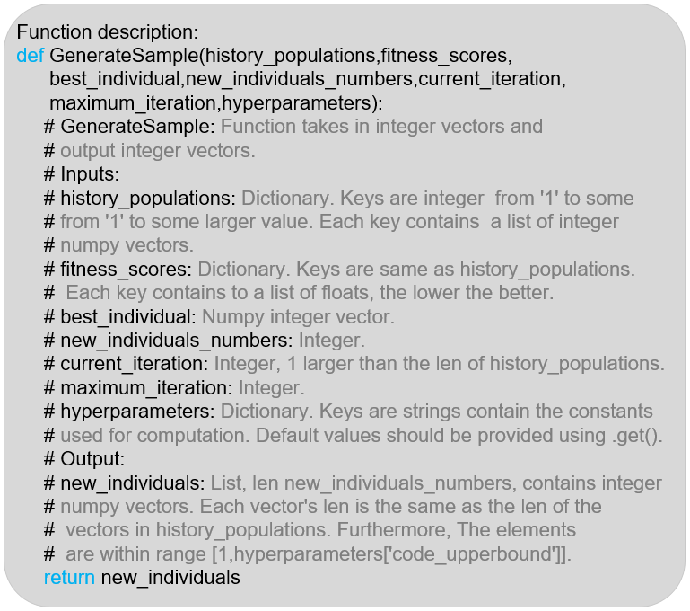
In Figure 2, we illustrate the algorithm description text for LLMs. This text will be prepended to the main body of all the prompts to help LLMs become familiar with the target of the algorithm. Here, we directly show LLMs the code. Due to the complexity in GenerateSamples, involving too many oral descriptions would rather complicate the problem and raise code compilation failures when evaluating the algorithm. This would, in turn, diminish the efficiency of the method. On the other hand, since LLMs have been pre-trained on vast amounts of text data and many have been further fine-tuned on codes, it is natural that they can comprehend through reading codes and the comments, consequently generating the executable algorithms for plug-and-play evaluation. In the following, we will describe the details in Algorithm 2.
Algorithms pool initialization. In this context, ‘pool’ denotes a set or a container comprising various clusters of algorithms. Each of these clusters has a grouping of codes of different TN-SS algorithms that are methodologically similar, along with their corresponding fitness scores.
We start by initializing the pool with the codes of three different well-developed TN-SS algorithms: the evolutionary-based method (Li & Sun, 2020), the local-sampling-based method (Li et al., 2022) and the greedy-based method. Besides, we evaluate these algorithms using the same strategy as we used to evaluate the new TN-SS algorithms.
Roulette selection. To determine which algorithms in the algorithms pool are selected as the in-context examples for the LLM-based crossover, we simulate the Russian roulette process. The intuition is that we want to maintain the diversity of the algorithm samples to prevent premature convergence. Given a set of individuals, let represent their ranking based on the fitness scores, the Russian roulette selection process performs the non-uniformly sampling over the set of individuals with each having the following probability:
| (2) |
Here, denotes a small value for numerical stability, the constant 0.01 is to avoid the domination of elite individuals and is the hyperparameter. Smaller indicates a stronger preference for the elite individuals and vice versa.
In our context, we conduct roulette selection on the clusters, followed by selecting algorithms within the chosen cluster. We repeat this process until the sample requirements are met. For selecting the clusters, we consider the fitness score of the best algorithm in each cluster as the cluster’s fitness score. We use and to denote the hyperparameters in the clusters and algorithms selection process respectively.

Construction of crossover prompt. After selecting algorithms, we concatenate them with the corresponding fitness scores as in-context crossover examples. As shown in Figure 3, we add the detail commands at the last line instructing the LLMs to generate an additional algorithms. This instruction is designed with the expectation that LLMs will analyze and fuse the successful experiences from the real-world executed examples and at the same time prevent the meaningless stacking of methods.

Finally, the crossover instruction is followed by the output instruction shown in Figure 4. This instruction is designed to rectify the final output of LLMs. For example, cutting the output of unnecessary analyses and appointing the output format for the codes. Moreover, we also add some instructions about code writing to ensure no compilation failures when evaluating. However, these parts are designed based on the trial-and-error interaction with LLMs which are LLM-dependent, and also depend on how we write the code, thus it has no unique standard.

Construction of mutation prompt. In the mutation step, TN-SS algorithms are received from the crossover step. We concatenate them as in-context examples. In Figure 5, we illustrate the details of the mutation instruction. Through prompting the LLMs, we discover potential enhancements in code efficiency, readability, and parallelism. However, these do not make essential improvements. Thus, to avoid these, we incorporate specific instructions that guide the mutation process away from them. Finally, the instruction in Figure 4 is appended to guide the output of LLMs.

Manage the generated algorithm samples. In this step, we need to classify the algorithms in into the existing algorithm clusters following a similar procedure as in the QD methods (Pugh et al., 2016). Instead of crafting a specific descriptor for diverse methodologies, we utilize the embedded knowledge in LLMs to address this task with the population management prompt as shown in Figure 6. Specifically, we choose the best performance algorithm in each cluster as the in-context examples. After prompting, we will get an index for classifying the new algorithm and we repeat this process until all algorithms in have been sorted.
Create novel algorithm cluster. To enhance the designed algorithms’ performance, incorporating diverse methodologies in design is crucial as it helps reduce bias. In this step, before reaching the maximum cluster number , we use the instruction in Figure 7 with the function description in Figure 2 and the output instruction in Figure 4 to guide LLM to create a novel algorithm. The in-context examples here are the same as the last step.

4 Experimental Results
In the experiment section, we utilize real-world data to showcase the TN-SS algorithm design capabilities of the GPTN-SS. Our primary focus is on evaluating whether the proposed method can effectively identify superior algorithms for TN-SS on the training data, and then extend this enhanced performance to novel, previously unseen cases.
4.1 Natural Images Compression
In the following section, we conduct the natural image compression task to evaluate whether the proposed GPTN-SS is capable of effectively designing high-quality algorithms for TN-SS. We specifically selected 14 natural images at random from the BSD500 dataset (Arbelaez et al., 2010). These images are initially grayscaled, resized by , and then reshaped into order-8 tensors by the trivial reshaping operations. Furthermore, we have divided the images into two parts: four for training and ten for testing. This indicates that we will evaluate the fitness scores of the designed algorithms using the four training images while running the GPTN-SS algorithm. Subsequently, we will evaluate the generalizability of the elite algorithms discovered through conducting TN-SS on the ten testing images.


| Images | Log compression ratio RSE – CR(RSE) | |||||
|---|---|---|---|---|---|---|
| TNGA | TNLS | Greedy | New-1 | New-2 | New-3 | |
| Train | 1.478 (0.128) | 1.419 (0.119) | 1.459 (0.125) | 1.436 (0.120) | 1.496 (0.124) | 1.446 (0.121) |
| Test | 1.332 (0.132) | 1.335 (0.131) | 1.309 (0.133) | 1.329 (0.129) | 1.352 (0.130) | 1.322 (0.129) |
| TGP | TNGA | TNLS | New-1 | New-2 | New-3 | |
|---|---|---|---|---|---|---|
| CCPP | 2.64 (0.06) [N/A] | 2.36 (0.06) [1900] | 2.50 (0.06) [1900] | 2.60 (0.06) [1900] | 2.24 (0.06) [1600] | 2.74 (0.06) [1300] |
| MG | 3.36 (0.33) [N/A] | 12.69 (0.33) [8400] | 17.25 (0.33) [7600] | 6.81 (0.33) [9200] | 3.01 (0.33) [10000] | 27.74 (0.33) [8400] |
Experiment setup. Here, we implement three SOTA sample-based TN-SS algorithms for comparison: the TNGA (Li & Sun, 2020), the TNLS (Li et al., 2022), and the Greedy method (Hashemizadeh et al., 2020). Note that the original TNGA and TNLS specifically target the TN-TS and TN-PS sub-problems of TN-SS, respectively. For a fair comparison, we have extended their capabilities. Specifically, we allow TNGA to search the formats and ranks simultaneously by relaxing the binary constraint. For TNLS, we set the TN template to fully-connected graph and focused on searching the optimal TN-ranks. In the greedy method, we implement a slightly modified approach. This may enhance performance by finding a better solution. It involves incrementally increasing or decreasing each element of the current best solution by one in each sampling step, then selecting the optimal edge for modification by evaluating it using Equation 1.
For the parameter settings of TNGA, the elimination rate is set as . Moreover, we set and (Li & Sun, 2020). The chance for each gene to mutate after the recombination is . For TNLS, we set (Li et al., 2022). In evaluating structure using Equation 1, we chose and applied the differentiable programming method (Liao et al., 2019) for computing TN-cores and evaluating RSE, initializing TN-cores with elements independently sampled from a Gaussian distribution . We employ the Adam optimizer with a learning rate of 0.01, running for 40,000 iterations (Kingma & Ba, 2014). Our rank search upper limit is 4, using 100 samples for all algorithms except the greedy method which maintains a constant sample number. Each algorithm runs for 20 iterations. The initial samples start with setting TN-ranks as close to one as possible to reduce computational demands. Specifically, there’s only a chance for any TN-rank to be 2. To ensure fairness, all algorithms will share the same initial samples. For the parameter settings of GPTN-SS, we set , , , and . Moreover, we choose gpt-4-1106-preview as the LLM model with a sample temperature of for all the prompting. The evaluation of the designed algorithms follows the same details as other algorithms described above.
Results. We present the results from the top three algorithms designed by GPTN-SS, namely New-1, New-2, and New-3, with fitness scores of 0.1216, 0.1220, and 0.1229, respectively. Among these, two have lower fitness scores compared to the best scores achieved by the SOTA algorithms. For reference, the fitness scores for TNGA, TNLS, and Greedy are 0.1273, 0.1223, and 0.1257, respectively. In Figure 8, we present the fitness curves generated by various algorithms applied to the training images. It can be seen from images 2, 3, and 4 that the designed algorithms exhibit competitive performance compared to the previous algorithms. Our analysis reveals that these algorithms establish an evolutionary framework with modified operations to better balance exploration and exploitation. This is achieved by leveraging the insights gained from previous algorithms and the embedded knowledge in LLMs.
Specifically, these algorithms incorporate all the historical solutions and introduce a more balanced ’parents’ selection strategy for generating ’off-springs’. These strategies, crucial for effective exploration, are novel additions not found in previous TN-SS algorithms and originate from LLMs. The exploration of New-1, beyond LLMs, benefits from previous knowledge. It employs a weight update strategy akin to TNLS (Li et al., 2022), with a progressively increasing mutation rate to enhance exploration. Besides, different methods utilize various strategies for exploitation, incorporating insights from the TNLS approach. New-1 enhances the process by stacking the optimal solution among the ’off-springs’. In contrast, New-3 always includes one of the ’parents’ as the best solution. Notably, New-2 introduces an innovative Gaussian perturbation mutation strategy, which may enhance the method’s exploitation capabilities. In comparison, New-3’s consistent use of the best solution may reduce its exploratory ability, which could explain the differences in performance observed when compared with other designed algorithms. The fitness curves of different algorithms applied to the testing images are shown in Figure 9. It can be concluded that the designed algorithms continue to demonstrate superior performance on unseen natural images. Specifically, for images 1, 2, 4, 7 and 8, they successfully find the deeper ’valley’ of the problem landscape than the previous algorithms.
In Table 1, we show the average log compression ratio (CR) (using base 10 logarithms) and the Relative Squared Error (RSE) for various algorithms’ learned structures across different images. As we can see, New-2 learns more expressive structures on the testing images than the previous algorithms.
4.2 Model Compression
In this experiment, our goal is to demonstrate the effectiveness of the GPTN-SS designed algorithms in compressing the model parameters of the learning tasks. Specifically, we compress the well-trained tensor train decomposition represented variational mean of the tensorial Gaussian process (TGP) (Izmailov et al., 2018), focusing on regression tasks of CCPP (Tüfekci, 2014) and MG (Flake & Lawrence, 2002). The tensors for CCPP and MG are 4 and 6 order, with mode dimensions of 12 and 8 respectively.
Experiment setup. Here, we perform TN-SS on the tensorial variational means using the previous TN-SS algorithms, New-1, New-2 and New-3. After compressing the tensors, we re-plug them into the TGP model to perform inference. Subsequently, we calculate and report the corresponding mean square error (MSE). The detail algorithm settings are the same as the natural image compression experiment except for the rank search upper bound is set at 10, the Adam learning rate is 0.001 and the core tensor is initialized using a Gaussian distribution with a variance of 0.01. Additionally, the CCPP’s value is , and for MG, it’s . The sample size for MG is 200, and it runs for 50 iterations.
Results. In Table 2, we demonstrate the number of the parameters of the learned TN representation and the corresponding MSE by different algorithms. The results of Greedy are not demonstrated in the table, since we find its learned structures fail in the inference. As the table illustrates, New-2 outperforms other algorithms, particularly in the MG dataset. While all approaches struggle to learn a lower parameter representation in this dataset, New-2 still manages to learn a more expressive structure compared to the original TGP model. This suggests that the novel TN structure searching strategy introduced by New-2 strikes a better balance between exploration and exploitation, leading to superior results.
Concluding Remarks and Limitation
Our experiential results confirm the positive impact of LLMs on TN-SS. Specifically, the proposed GPTN-SS method can leverage insights gained from the existing algorithms and the embedded knowledge in LLMs to automatically discover novel TN-SS algorithms that achieve a better balance between exploration and exploitation. The real-world applications of image compression and model parameters compression demonstrate the superiority and the generalizability of the discovered algorithms in finding better TN structures.
Limitation. A primary limitation of our method is that the final discovered algorithms’ performance is subject to variation due to changes in LLMs. Nonetheless, we anticipate a positive correlation between the performance of designed algorithms by our method and the capabilities of LLMs.
References
- Acharya et al. (2022) Acharya, A., Rudolph, M., Chen, J., Miller, J., and Perdomo-Ortiz, A. Qubit seriation: Improving data-model alignment using spectral ordering. arXiv preprint arXiv:2211.15978, 2022.
- Achiam et al. (2023) Achiam, J., Adler, S., Agarwal, S., Ahmad, L., Akkaya, I., Aleman, F. L., Almeida, D., Altenschmidt, J., Altman, S., Anadkat, S., et al. Gpt-4 technical report. arXiv preprint arXiv:2303.08774, 2023.
- Anandkumar et al. (2014) Anandkumar, A., Ge, R., Hsu, D., Kakade, S. M., and Telgarsky, M. Tensor decompositions for learning latent variable models. The Journal of Machine Learning Research, 15(1):2773–2832, 2014.
- Arbelaez et al. (2010) Arbelaez, P., Maire, M., Fowlkes, C., and Malik, J. Contour detection and hierarchical image segmentation. IEEE transactions on pattern analysis and machine intelligence, 33(5):898–916, 2010.
- Blocklove et al. (2023) Blocklove, J., Garg, S., Karri, R., and Pearce, H. Chip-chat: Challenges and opportunities in conversational hardware design. arXiv preprint arXiv:2305.13243, 2023.
- Boiko et al. (2023) Boiko, D. A., MacKnight, R., Kline, B., and Gomes, G. Autonomous chemical research with large language models. Nature, 624(7992):570–578, 2023.
- Bubeck et al. (2023) Bubeck, S., Chandrasekaran, V., Eldan, R., Gehrke, J., Horvitz, E., Kamar, E., Lee, P., Lee, Y. T., Li, Y., Lundberg, S., et al. Sparks of artificial general intelligence: Early experiments with gpt-4. arXiv preprint arXiv:2303.12712, 2023.
- Cai et al. (2023) Cai, T., Wang, X., Ma, T., Chen, X., and Zhou, D. Large language models as tool makers. arXiv preprint arXiv:2305.17126, 2023.
- Cai & Li (2021) Cai, Y. and Li, P. A blind block term decomposition of high order tensors. In Proceedings of the AAAI Conference on Artificial Intelligence, number 8, pp. 6868–6876, 2021.
- Chen et al. (2023) Chen, A., Dohan, D. M., and So, D. R. Evoprompting: Language models for code-level neural architecture search. arXiv preprint arXiv:2302.14838, 2023.
- Chen et al. (2022) Chen, Z., Lu, J., and Zhang, A. R. One-dimensional tensor network recovery. arXiv preprint arXiv:2207.10665, 2022.
- Cheng et al. (2020) Cheng, Z., Li, B., Fan, Y., and Bao, Y. A novel rank selection scheme in tensor ring decomposition based on reinforcement learning for deep neural networks. In ICASSP 2020-2020 IEEE International Conference on Acoustics, Speech and Signal Processing (ICASSP), pp. 3292–3296. IEEE, 2020.
- Cichocki et al. (2016) Cichocki, A., Lee, N., Oseledets, I., Phan, A.-H., Zhao, Q., Mandic, D. P., et al. Tensor networks for dimensionality reduction and large-scale optimization: Part 1 low-rank tensor decompositions. Foundations and Trends® in Machine Learning, 9(4-5):249–429, 2016.
- Cichocki et al. (2017) Cichocki, A., Phan, A.-H., Zhao, Q., Lee, N., Oseledets, I., Sugiyama, M., Mandic, D. P., et al. Tensor networks for dimensionality reduction and large-scale optimization: Part 2 applications and future perspectives. Foundations and Trends® in Machine Learning, 9(6):431–673, 2017.
- Creswell et al. (2022) Creswell, A., Shanahan, M., and Higgins, I. Selection-inference: Exploiting large language models for interpretable logical reasoning. arXiv preprint arXiv:2205.09712, 2022.
- Falcó et al. (2023) Falcó, A., Hackbusch, W., and Nouy, A. Geometry of tree-based tensor formats in tensor banach spaces. Annali di Matematica Pura ed Applicata (1923-), pp. 1–18, 2023.
- Flake & Lawrence (2002) Flake, G. W. and Lawrence, S. Efficient SVM regression training with SMO. Machine Learning, 46(1):271–290, 2002.
- Ghadiri et al. (2023) Ghadiri, M., Fahrbach, M., Fu, G., and Mirrokni, V. Approximately optimal core shapes for tensor decompositions. arXiv preprint arXiv:2302.03886, 2023.
- Glasser et al. (2019) Glasser, I., Sweke, R., Pancotti, N., Eisert, J., and Cirac, I. Expressive power of tensor-network factorizations for probabilistic modeling. Advances in neural information processing systems, 32, 2019.
- Haberstich et al. (2021) Haberstich, C., Nouy, A., and Perrin, G. Active learning of tree tensor networks using optimal least-squares. arXiv preprint arXiv:2104.13436, 2021.
- Haghshenas et al. (2022) Haghshenas, R., Gray, J., Potter, A. C., and Chan, G. K.-L. Variational power of quantum circuit tensor networks. Physical Review X, 12(1):011047, 2022.
- Haluptzok et al. (2022) Haluptzok, P., Bowers, M., and Kalai, A. Language models can teach themselves to program better. arxiv 2022. arXiv preprint arXiv:2207.14502, 2022.
- Hashemizadeh et al. (2020) Hashemizadeh, M., Liu, M., Miller, J., and Rabusseau, G. Adaptive learning of tensor network structures. arXiv preprint arXiv:2008.05437, 2020.
- Hawkins & Zhang (2021) Hawkins, C. and Zhang, Z. Bayesian tensorized neural networks with automatic rank selection. Neurocomputing, 453:172–180, 2021.
- Hayashi et al. (2019) Hayashi, K., Yamaguchi, T., Sugawara, Y., and Maeda, S.-i. Exploring unexplored tensor network decompositions for convolutional neural networks. In Advances in Neural Information Processing Systems, pp. 5553–5563, 2019.
- Hemberg et al. (2024) Hemberg, E., Moskal, S., and O’Reilly, U.-M. Evolving code with a large language model. arXiv preprint arXiv:2401.07102, 2024.
- Hikihara et al. (2023) Hikihara, T., Ueda, H., Okunishi, K., Harada, K., and Nishino, T. Automatic structural optimization of tree tensor networks. Physical Review Research, 5(1):013031, 2023.
- Izmailov et al. (2018) Izmailov, P., Novikov, A., and Kropotov, D. Scalable Gaussian processes with billions of inducing inputs via tensor train decomposition. In International Conference on Artificial Intelligence and Statistics, pp. 726–735. PMLR, 2018.
- Kingma & Ba (2014) Kingma, D. P. and Ba, J. Adam: A method for stochastic optimization. arXiv preprint arXiv:1412.6980, 2014.
- Kodryan et al. (2023) Kodryan, M., Kropotov, D., and Vetrov, D. Mars: Masked automatic ranks selection in tensor decompositions. In International Conference on Artificial Intelligence and Statistics, pp. 3718–3732. PMLR, 2023.
- Kossaifi et al. (2020) Kossaifi, J., Lipton, Z. C., Kolbeinsson, A., Khanna, A., Furlanello, T., and Anandkumar, A. Tensor regression networks. Journal of Machine Learning Research, 21:1–21, 2020.
- Lehman et al. (2023) Lehman, J., Gordon, J., Jain, S., Ndousse, K., Yeh, C., and Stanley, K. O. Evolution through large models. In Handbook of Evolutionary Machine Learning, pp. 331–366. Springer, 2023.
- Li & Sun (2020) Li, C. and Sun, Z. Evolutionary topology search for tensor network decomposition. In International Conference on Machine Learning, pp. 5947–5957. PMLR, 2020.
- Li et al. (2022) Li, C., Zeng, J., Tao, Z., and Zhao, Q. Permutation search of tensor network structures via local sampling. In International Conference on Machine Learning, pp. 13106–13124. PMLR, 2022.
- Li et al. (2023) Li, C., Zeng, J., Li, C., Caiafa, C. F., and Zhao, Q. Alternating local enumeration (tnale): Solving tensor network structure search with fewer evaluations. In International Conference on Machine Learning, pp. 20384–20411. PMLR, 2023.
- Li et al. (2021) Li, N., Pan, Y., Chen, Y., Ding, Z., Zhao, D., and Xu, Z. Heuristic rank selection with progressively searching tensor ring network. Complex & Intelligent Systems, pp. 1–15, 2021.
- Liao et al. (2019) Liao, H.-J., Liu, J.-G., Wang, L., and Xiang, T. Differentiable programming tensor networks. arXiv preprint arXiv:1903.09650, 2019.
- Liu et al. (2023a) Liu, F., Tong, X., Yuan, M., and Zhang, Q. Algorithm evolution using large language model. arXiv preprint arXiv:2311.15249, 2023a.
- Liu et al. (2023b) Liu, P., Yuan, W., Fu, J., Jiang, Z., Hayashi, H., and Neubig, G. Pre-train, prompt, and predict: A systematic survey of prompting methods in natural language processing. ACM Computing Surveys, 55(9):1–35, 2023b.
- Liu et al. (2023c) Liu, S., Chen, C., Qu, X., Tang, K., and Ong, Y.-S. Large language models as evolutionary optimizers. arXiv preprint arXiv:2310.19046, 2023c.
- Liu et al. (2023d) Liu, Y., Lu, Y., Ou, W., Long, Z., and Zhu, C. Adaptively topological tensor network for multi-view subspace clustering. arXiv preprint arXiv:2305.00716, 2023d.
- Long et al. (2021) Long, Z., Zhu, C., Liu, J., and Liu, Y. Bayesian low rank tensor ring for image recovery. IEEE Transactions on Image Processing, 30:3568–3580, 2021.
- Markov & Shi (2008) Markov, I. L. and Shi, Y. Simulating quantum computation by contracting tensor networks. SIAM Journal on Computing, 38(3):963–981, 2008.
- Meyerson et al. (2023) Meyerson, E., Nelson, M. J., Bradley, H., Moradi, A., Hoover, A. K., and Lehman, J. Language model crossover: Variation through few-shot prompting. arXiv preprint arXiv:2302.12170, 2023.
- Mickelin & Karaman (2020) Mickelin, O. and Karaman, S. On algorithms for and computing with the tensor ring decomposition. Numerical Linear Algebra with Applications, 27(3):e2289, 2020.
- Miller et al. (2021) Miller, J., Rabusseau, G., and Terilla, J. Tensor networks for probabilistic sequence modeling. In International Conference on Artificial Intelligence and Statistics, pp. 3079–3087. PMLR, 2021.
- Nasir et al. (2023) Nasir, M. U., Earle, S., Togelius, J., James, S., and Cleghorn, C. Llmatic: Neural architecture search via large language models and quality-diversity optimization. arXiv preprint arXiv:2306.01102, 2023.
- Nie et al. (2021) Nie, C., Wang, H., and Tian, L. Adaptive tensor networks decomposition. In BMVC, 2021.
- Noorbakhsh et al. (2021) Noorbakhsh, K., Sulaiman, M., Sharifi, M., Roy, K., and Jamshidi, P. Pretrained language models are symbolic mathematics solvers too! arXiv preprint arXiv:2110.03501, 2021.
- Nori et al. (2023) Nori, H., King, N., McKinney, S. M., Carignan, D., and Horvitz, E. Capabilities of gpt-4 on medical challenge problems. arXiv preprint arXiv:2303.13375, 2023.
- Novikov et al. (2015) Novikov, A., Podoprikhin, D., Osokin, A., and Vetrov, D. P. Tensorizing neural networks. In Advances in Neural Information Processing Systems, pp. 442–450, 2015.
- Orús (2014) Orús, R. A practical introduction to tensor networks: Matrix product states and projected entangled pair states. Annals of Physics, 349:117–158, 2014.
- Orús (2019) Orús, R. Tensor networks for complex quantum systems. Nature Reviews Physics, 1(9):538–550, 2019.
- Pugh et al. (2016) Pugh, J. K., Soros, L. B., and Stanley, K. O. Quality diversity: A new frontier for evolutionary computation. Frontiers in Robotics and AI, 3:40, 2016.
- Rai et al. (2014) Rai, P., Wang, Y., Guo, S., Chen, G., Dunson, D., and Carin, L. Scalable bayesian low-rank decomposition of incomplete multiway tensors. In International Conference on Machine Learning, pp. 1800–1808. PMLR, 2014.
- Richter et al. (2021) Richter, L., Sallandt, L., and Nüsken, N. Solving high-dimensional parabolic pdes using the tensor train format. In International Conference on Machine Learning, pp. 8998–9009. PMLR, 2021.
- Romera-Paredes et al. (2023) Romera-Paredes, B., Barekatain, M., Novikov, A., Balog, M., Kumar, M. P., Dupont, E., Ruiz, F. J., Ellenberg, J. S., Wang, P., Fawzi, O., et al. Mathematical discoveries from program search with large language models. Nature, pp. 1–3, 2023.
- Sedighin et al. (2021) Sedighin, F., Cichocki, A., and Phan, A.-H. Adaptive rank selection for tensor ring decomposition. IEEE Journal of Selected Topics in Signal Processing, 15(3):454–463, 2021.
- Solgi et al. (2022) Solgi, R., Loaiciga, H. A., and Zhang, Z. Evolutionary tensor train decomposition for hyper-spectral remote sensing images. In IGARSS 2022-2022 IEEE International Geoscience and Remote Sensing Symposium, pp. 1145–1148. IEEE, 2022.
- Stoudenmire & Schwab (2016) Stoudenmire, E. and Schwab, D. J. Supervised learning with tensor networks. In Advances in Neural Information Processing Systems, pp. 4799–4807, 2016.
- Tian et al. (2023) Tian, H., Lu, W., Li, T. O., Tang, X., Cheung, S.-C., Klein, J., and Bissyandé, T. F. Is chatgpt the ultimate programming assistant–how far is it? arXiv preprint arXiv:2304.11938, 2023.
- Tüfekci (2014) Tüfekci, P. Prediction of full load electrical power output of a base load operated combined cycle power plant using machine learning methods. International Journal of Electrical Power & Energy Systems, 60:126–140, 2014.
- Vaswani et al. (2017) Vaswani, A., Shazeer, N., Parmar, N., Uszkoreit, J., Jones, L., Gomez, A. N., Kaiser, Ł., and Polosukhin, I. Attention is all you need. Advances in neural information processing systems, 30, 2017.
- Wei et al. (2022a) Wei, J., Tay, Y., Bommasani, R., Raffel, C., Zoph, B., Borgeaud, S., Yogatama, D., Bosma, M., Zhou, D., Metzler, D., et al. Emergent abilities of large language models. arXiv preprint arXiv:2206.07682, 2022a.
- Wei et al. (2022b) Wei, J., Wang, X., Schuurmans, D., Bosma, M., Xia, F., Chi, E., Le, Q. V., Zhou, D., et al. Chain-of-thought prompting elicits reasoning in large language models. Advances in Neural Information Processing Systems, 35:24824–24837, 2022b.
- Yang et al. (2023) Yang, C., Wang, X., Lu, Y., Liu, H., Le, Q. V., Zhou, D., and Chen, X. Large language models as optimizers. arXiv preprint arXiv:2309.03409, 2023.
- Yin et al. (2022) Yin, M., Phan, H., Zang, X., Liao, S., and Yuan, B. Batude: Budget-aware neural network compression based on Tucker decomposition. In Proceedings of the AAAI Conference on Artificial Intelligence, volume 1, 2022.
- Yokota et al. (2016) Yokota, T., Zhao, Q., and Cichocki, A. Smooth PARAFAC decomposition for tensor completion. IEEE Transactions on Signal Processing, 64(20):5423–5436, 2016.
- Zhang et al. (2023a) Zhang, M. R., Desai, N., Bae, J., Lorraine, J., and Ba, J. Using large language models for hyperparameter optimization. arXiv e-prints, pp. arXiv–2312, 2023a.
- Zhang et al. (2023b) Zhang, S., Gong, C., Wu, L., Liu, X., and Zhou, M. Automl-gpt: Automatic machine learning with gpt. arXiv preprint arXiv:2305.02499, 2023b.
- Zhao et al. (2015) Zhao, Q., Zhang, L., and Cichocki, A. Bayesian CP factorization of incomplete tensors with automatic rank determination. IEEE transactions on pattern analysis and machine intelligence, 37(9):1751–1763, 2015.
- Zheng et al. (2023a) Zheng, M., Su, X., You, S., Wang, F., Qian, C., Xu, C., and Albanie, S. Can gpt-4 perform neural architecture search? arXiv preprint arXiv:2304.10970, 2023a.
- Zheng et al. (2023b) Zheng, Y.-B., Zhao, X.-L., Zeng, J., Li, C., Zhao, Q., Li, H.-C., and Huang, T.-Z. Svdinstn: An integrated method for tensor network representation with efficient structure search. arXiv preprint arXiv:2305.14912, 2023b.
- Zhu et al. (2023) Zhu, Z., Xue, Y., Chen, X., Zhou, D., Tang, J., Schuurmans, D., and Dai, H. Large language models can learn rules. arXiv preprint arXiv:2310.07064, 2023.
