Market proliferation and the impact of locational complexity on network restructuring

The measure for supply chain structural complexity used in this manuscript is built around a collection $\wp$ of triplets $\left\{SKU,Market,Channel\right\}$ that characterise the flow of products in a firm’s supply chain. Each of these triplets, referred to as pars (plural partes) has associated a probability value $p_{i}\in\left(0,1\right)$ that represents the likelihood that a money unit of revenue comes from the sell by triplet $i\in\wp$. With these elements, we define system’s $\wp$ pars-complexity as

where $\mathbf{p}$ is the vector of weights, $p_{i}$, for $i=1,\ldots,\left|\wp\right|$, satisfying $\sum_{i\in\wp}p_{i}=1$.

Function $C_{p}\left(\mathbf{p}\right)$ satisfies the following properties:

1. 1.

   $C_{p}\left(\mathbf{p}\right)$ is continuous and concave in $p$.

2. 2.

   If $\left|\wp\right|=1$, then the system’s complexity is zero, i.e. $C_{p}\left(\mathbf{p}\right)=0$.

3. 3.

   $C_{p}$ attains a maximum when $p_{i}=\frac{1}{\ \left|\wp\right|}$ for all $i=1,\ ...,\left|\wp\right|$. Such maximum is equal to $\log_{2}{\left(\left|\wp\right|\right)}$.

Proof of this properties, together with a discussion around the attributes of the pars-complexity measure, can be found in Ruiz-Hernández et al. [9].

The pars-complexity metric is simply Shannon’s measure of information [52]: the expected quantity of information necessary to describe a system’s state. As described by Ruiz-Hernández et al. [9], the metric quantifies the information generated by the flow of goods and services in the supply chain, and can thus be used as a proxi for the structural complexity of a supply chain.

To put the structural complexity problem within a locational complexity framework, we consider a distribution network $\mathcal{S}$ where a central manager coordinates a number of regional or local facilities (retail or local distribution centres) serving a set $\mathcal{N}$ of demand nodes. For the sake of simplicity and without any loss of generality, we assume $\mathcal{S}\subset\mathcal{N}$. Each regional facility $\ell$ serves a subset $\mathcal{N}_{\ell}$ of demand nodes, where $\mathcal{N}_{\ell}=\left\{i\in\mathcal{N}:d\left(i,\ell\right)\leq\inf_{\ell^{\prime}\in\mathcal{S}}\left\{d\left(i,\ell^{\prime}\right)\right\}\right\}$ for $\ell\in\mathcal{S}$. Let $\mathcal{N}^{\mathcal{S}}$ represent the collection of allocation sets, $\mathcal{N}_{\ell}$, associated to all facilities $\ell$ in distribution network $\mathcal{S}$.

Assuming that each demand node $i\in\mathcal{N}$ contributes a proportion $p_{i}$ of the total demand. The total complexity of system $\left\{\mathcal{N}^{\mathcal{S}},\mathcal{S}\right\}$ can be written as

where $q_{\ell}=\sum_{i\in\mathcal{N}_{\ell}}p_{i}$ represents the fraction of the total demand served by facility $\ell$; and $C_{p}\left(\mathcal{N}_{\ell},\ell\right)$ represents the complexity of the single-facility system $\left\{\mathcal{N}_{\ell},\ell\right\}$.

The first equality in Equation (2) expresses system $\mathcal{S}$’s pars-complexity in terms of the contributions of each demand node. The term after the second equal sign decomposes the total pars-complexity in two parts: the first element represents the pars-complexity faced by a (hypothetical) central manager, and the second one the weighted average of the pars-complexities of the local units.

A consequence of Properties 1 to 3 in a locational context, is that networks with the same number of nodes may have different $C_{p}$ values depending on the distribution of the demand accross the different nodes. Moreover, smaller networks may show higher complexity values than larger ones.

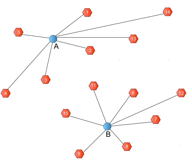
An illustrative example of the use of metric within the locational context is provided in Figure 3. Panel (a) in the figure shows a distribution network consisting of three facilities and fourteen demand nodes. The demand nodes are assigned to their closest server. In this network, $\mathcal{S}=\left\{A,B,C\right\}$; $\mathcal{N}_{A}=\left\{1,2,3,4,5\right\}$; $\mathcal{N}_{B}=\left\{6,7,8,9,10,11\right\}$; $\mathcal{N}_{C}=\left\{12,13,14\right\}$; and $\mathcal{N}^{\mathcal{S}}=\left\{\mathcal{N}_{A},\mathcal{N}_{B},\mathcal{N}_{C}\right\}$. The details of the calculation of $C_{p}\left(\mathcal{N}^{\mathcal{S}},\mathcal{S}\right)$ are presented in Table 2. The third column is used to compute the pars-complexity of the system according to the left-hand-side term in (2). The fourth column provides the contribution of each demand node to the associated facility, $q^{\ell}_{i}=\tfrac{p_{i}}{q_{\ell}},\,\forall i\in\mathcal{N}_{\ell},\ell\in\mathcal{S}$. Finally, the last column provides the elements for computing $C_{p}$ as indicated by the right-hand-side term of equation (2).

Panel (b) in Figure 3 shows a restructuring of the network presented in panel (a), where facility $C$ is removed and its associated nodes allocated to their second closest facility: $A$ for nodes $13$ and $14$; and $B$ for node $12$. It can be verified that while the total system’s complexity remains the same ($C_{p}=3.624$), the complexities of the remaining facilities change from $C_{p}\left(\mathbf{q}^{A}\right)=2.202$ and $C_{p}\left(\mathbf{q}^{B}\right)=2.460$ to $2.563$ and $2.697$, respectively. Likewise, the central manager’s $C_{p}$ value (quantity $S1$ in Table 2) changes from $1.485$ to $0.984$.

It has been argued [8, 1, 11] that supply chain complexity introduces hidden costs that erode the company’s capability for generating profits. In an empirical study, Menezes et al. [23] found that structural complexity can have an impact in operational profit between 2% and 10% per pars-complexity point. Previously, Scheiter et al. [16] estimated that reducing complexity may lead to an increase of 3 to 5% in EBIT. In this section we present a mathematical expression for the company’s profit that takes into account the effect of complexity. For completeness, in the following lines we present the main notation used throughout this manuscript.

Assuming that pars-complexity imposes a penalty (or hidden cost) on benefits represented by parameter $0\leq\alpha<1$, the gross profit earned by a network consisting of $\left|\mathcal{S}\right|$ facilities is given by

where

represents the sum of the profits earned by regional facility $\ell$ when serving all the assigned demand nodes, $i\in\mathcal{N}_{\ell}$.

Each demand node’s profit is defined as the difference between the revenue per unit, $r$, and the unit transport cost, $\gamma d\left(i,\ell\right)$, multiplied by the node’s demand, $W_{i}$. Parameter $\gamma$ represents the transport cost per distance and product unit.

Expressions (3) and (4) presume a perfectly competitive market where prices and demand are exogenous (and constant); and the revenue per unit, $r$, is net of production costs. Transport costs are also fixed and distances are invariant. It is also assumed that parameter $\alpha$ is constant and known, satisfying $1-\alpha C_{p}\left(\mathcal{N}^{\mathcal{S}},\mathcal{S}\right)\ll 1$.

Using (3), we define the cost of complexity for system $\left\{\mathcal{N}^{\mathcal{S}},\mathcal{S}\right\}$ as

Additionally, expressions (3) and (5) can be easily generalised to the case where the cost of complexity is different for each facility by simply defining independent $\alpha_{\ell}$ values for each facility $\ell\in\mathcal{S}$.

The objective of the decision problem is to find the optimal number and location of facilities, and the associated demand allocation, to maximise the firm’s profit when considering the cost of complexity.

We first introduce the optimisation problem for a given number $K$ of facilities. We refer to this as the $K$-MedianPlex problem. Using $\mathcal{S}$ for a given set of open facilities, and $\phi_{\ell}$ for the fix opening/operating cost of facility $\ell\in\mathcal{S}$, our problem can be written as:

where $\Pi^{\circ}\left(\mathcal{N}^{\mathcal{S}},\mathcal{S}\right)$ is given by equation (3). Please notice that when using expression $\Pi^{\circ}\left(\mathcal{N}^{\mathcal{S}},\mathcal{S}\right)$, the local complexity, $C_{p}\left(\mathcal{N}_{\ell},\ell\right)$, is obtained by using the contribution of each demand node to local demand served by facility $\ell$, i.e. $q^{\ell}_{i}=\dfrac{W_{i}}{\sum_{h\in\mathcal{N}_{\ell}}W_{h}}$ for all $i\in\mathcal{N}_{\ell}$. Constraint (7), the cardinal of set $\mathcal{S}$, indicates the number of open facilities; and constraints (8) impose that each demand node should be allocated to only one facility and guarantees that all nodes are allocated.

It can be seen that the $K$-MedianPlex problem is a non-linear variant of a $K$-Median problem with fixed costs:

We use $\mathcal{S}^{K}$ to represent the optimal solution to problem (9) when the number of open facilities is $K$. Solving the $K$-MedianPlex problem for different values of $K$ allows finding the number and location of facilities that maximises the firm’s profit under the presence of structural complexity.

The $K$-MedianPlex problem presents high computational complexity. It is a non-linear, highly combinatorial problem, hardly solvable for real-sized problems. However, structural complexity is not, in general, a design problem, but a consequence of successive network expansions aimed at reaching higher profitability. This is aligned with the objective of this work which, rather than finding the optimal solution to the $Z^{K}_{Plex}$ problem, seeks to identify the reasons why network restructuring efforts may fail at reducing operating costs; and to assess the possibility of reducing the burden of complexity in a network. With the second objective in mind, we propose the following $Z^{\circ}_{Plex}$ function, which can be used to find the net profit of any distribution network $\left\{\mathcal{N}^{\mathcal{S}},\mathcal{S}\right\}$:

Without any loss of generality, in what follows it is assumed that network $\mathcal{S}$ has been designed without taking into account the cost of complexity or, alternatively, that it is the product of successive expansions of a smaller network (we refer to this as organic growth).

It has been said that complexity introduces hidden costs that cripple the capacity of the firm for generating profits [17, 19]. In location decisions, additional costs required for connecting, supporting, and supplying the distribution network, may outweigh the increased revenues generated from the access to new markets and customers.

The $K$-MedianPlex problem formulation, represented by equations (6) to (8), together with equation (12), allow us to provide a visual characterisation of the burden of locational complexity. The top line in Figure 4 represents the forecasted profits implied from standard facility location models, in particular the $K$-Median problem, for different numbers of facilities. The bottom curve represents the actual profits. This curve is obtained by evaluating the current network configuration in equation (3). Finally, the intermediate curve represents the optimal solution to the $K$-MedianPlex problem. The distances between these curves represent two different components of the cost imposed by locational complexity on the company. First, there is an unavoidable cost of complexity. It is the cost imposed by the intricate interrelations existing in any distribution network. This cost is represented by the distance between the upper and the intermediate curves. The second one is the cost of ignoring the existence of complexity during network design, and it is represented by the distance between the intermediate and the bottom curves. This discussion will be recalled in Section 5 when proposing strategies aimed at alleviating the burden of complexity in network design.

Regarding the addiction to growth, complexity-driven costs are usually hidden in early design stages. This implies that the observed profit may be, in practice, smaller than the one forecasted during the planning process. If revenues are as expected, this may give the management the wrong impression that the optimal number of facilities may indeed be larger than initially planned. The natural reaction might be to further increase the number of facilities, aiming at reaching the profit levels forecasted by the analytical models. If this actually leads to an increase in profit, but the observed figures remain below the forecasted ones, the same reasoning can lead the company to unnecessary expansions in the network in the quest for the higher profit levels promised by the analytical models.

A simple numerical exercise, using the $K$-Median Plex objective function (6) with $\Pi^{\circ}\left(\mathcal{N}^{\mathcal{S}},\mathcal{S}\right)$ given by equation (3), and approximating the complexity cost $\alpha$ to 2.5% of the profits as suggested by Menezes et al. [23], provides support to this claim. Figure 5 depicts the solution to a number of $K$-Median problems, ranging from 1 to 15 facilities. The upper curve represents the total revenue associated to each solution. The forecasted and actual profits are represented by the two concave curves (left-hand side axis). The cost of complexity, the distance between the two profit curves, is represented by the dashed curve (right-hand side axis). It can be seen that a decision maker that focuses solely on revenue, may have a strong incentive to keep expanding his network in the quest for higher profit levels, ignoring that the company has grown beyond its optimal size.

Data from different retailers and banks evince that, despite large network reduction and restructuring efforts, their operating costs have either experienced only a minor reduction or remained almost constant. Straightforward manipulation of the pars-Complexity measure may provide insight for understanding this phenomenon.

A common feature of all these companies is that their service is universal, i.e. it targets all the regional demand and no client can be excluded. Therefore, irrespectively of the number of facilities, the target market remains the same. The reader can think, for example, of a convenience-stores chain that has three shops in a neighbourhood. In the absecne of competitors, closing one of their facilities will trigger a re-distribution of clients across the facilities that remain open, but the demand will remain fairly the same. The closing of bank branches, where the clients are simply allocated to a different branch is another example of this.

In order to bring this into the locational complexity framework, consider a centrally managed system $\mathcal{L}^{1}$ consisting of $K$ independent subsystems or regional distribution centres $\mathcal{S}^{1}_{1},\ldots,\mathcal{S}^{1}_{K}$. Each of these centres contributes a proportion $p^{1}_{\ell},\,\ell=1,\ldots,K$ of the total sales. These contributions are collected in vector $\mathbf{p}^{1}=\left(p^{1}_{1},\ldots,p^{1}_{K}\right)$. Likewise, each distribution centre $\mathcal{S}^{1}_{\ell}$ has associated a number $H_{\ell}$ of retailers, each contributing a proportion $q^{1,\ell}_{h}$ of the centre’s total sales. The weights vector of centre $\ell$ is represented by $\mathbf{q}^{1,\ell}=\left(q^{1,\ell}_{1},\ldots,q^{1,\ell}_{H_{\ell}}\right)$. The pars-Complexity of this system, represented by $C^{1}_{p}=C_{p}\left(\mathcal{L}^{1}\right)$, can be readily computed using the right hand side expression in (2). Consider an alternative configuration of the network, system $\mathcal{L}^{2}$, consisting of $M$ independent regional distribution centres, each of them serving a number $G_{m}$ of retailers. The corresponding weights vectors are $\mathbf{p}^{2}$ and $\mathbf{q}^{2,m},m=1,\ldots,M$. The pars-Complexity is represented by $C^{2}_{p}=C_{p}\left(\mathcal{L}^{2}\right)$. Assume also that $M\ll K$, and $N=\sum_{\ell=1}^{K}H_{\ell}=\sum_{m=1}^{M}G_{m}$ is the total number of retail centres.

The following proposition uses the convention $\oplus_{i=1}^{n}\mathbf{g}_{i}=\mathbf{g}^{1}||\mathbf{g}^{2}||\cdots||\mathbf{g}^{n}$ for representing the concatenation of vectors $\mathbf{g}^{1}$ to $\mathbf{g}^{n}$.

Proposition 1 provides an intuitive result that finds its foundation in the Second law of Thermodynamics (roughly speaking, the total entropy in a closed system can never decrease): if structural complexity is understood –as Ruiz-Hernández et al. [9] suggest- as an entropic process, then the level of complexity faced by a company will be the same as long as the target market remains unchanged, irrespective of the actual network configuration.

Therefore, as long as their market remains the same, companies that provide in-store services will hardly attain any reduction in complexity-related costs by simply eliminating intermediate distribution centres or local facilities. Moreover, the elimination of one centre (and the corresponding absorption of its associated demand by one or more facilities) may increase the total complexity of the facilities that remain open.

These results also suggest that the only mechanism that may bring a reduction in pars-Complexity, and therefore in operating costs, is a reduction in its market share. For the interested reader, [9] provides a mechanism for computing the market contribution at which the elimination of a certain demand node will surely reduce supply chain’s structural complexity.

In the following section we present three alternative mechanisms (two of them involving demand reduction) for reducing the burden of locational complexity in the supply chain.

Standard facility location and network design models ignore the hidden costs of channel and market proliferation. This strategy results in oversized networks whose profitability is often overestimated. This situation frequently leads companies to look for strategies aimed at improving their network’s performance [11]. In order to address this problem, in particular in situations where local facilities still appear profitable, it may seem intuitive to reduce the burden carried by the facilities that bear larger demand, and to cede market share to other facilities which currently carry a lighter load. We refer to this type of strategy as network rebalancing.

To assess the effectiveness of such policies, in this section we propose a strategy that, starting from a solution to the $K$-Median problem characterised by the pair $\left\{\mathcal{N}^{\mathcal{S}^{K}},\mathcal{S}^{K}\right\}$, reassigns demand nodes to different facilities exploiting trade-offs between increased transportation costs and reduced complexity penalties. The reassignment is conducted by sequentially selecting nodes in decreasing order of the total shipment cost to the second closest facility. If reallocating a node to its second closest facility brings an improvement in the objective function, the node is reallocated; otherwise, it remains assigned to its original facility. After demand reallocation, the algorithm takes one further improvement step by solving a $1$-Median problem for each of the available facilities and their associated nodes.

Pseudo-code for this reallocation and re-centring procedure is presented in A.1. A numerical assessment of the efficiency of this strategy is presented in Section 6.

Locational complexity is not typically result of network design, but a problem that arises from organic growth, i.e. from successive network expansions aimed at achieving growth in profits. Thus, in order to reduce complexity, firms may consider abandoning certain markets and concentrating their services in the most profitable regions (although this approach often finds resistance under the rationale that lost sales will affect profit negatively). To address this issue, we propose a network rationalisation strategy consisting of sequentially removing those demand nodes for which the savings from reducing complexity and transportation costs, offset the lost revenue and lead to an increase in profits.

The pseudo-code is presented in A.2. The algorithm starts from a given network configuration $\left\{\mathcal{N}^{\mathcal{S}^{K}},\mathcal{S}^{K}\right\}$ and takes, for each given facility $\ell\in\mathcal{S}^{K}$, a set with an arbitrary number of the most distant demand nodes in $\mathcal{N}_{\ell}$. We refer to this set as $\Theta_{\ell}$. For each node $i\in\Theta_{\ell}$, the algorithm computes the value of the $Z_{Plex}^{\circ}$ function (given by equation (12)), represented by $Z_{Plex}^{\circ}\left(\mathcal{N}^{\mathcal{S}^{K}}-\left\{i\right\},\mathcal{S}^{K}\right)$, which results from eliminating $i$ from $\mathcal{N}_{\ell}$ and computes the ratio

where $\widetilde{Z}_{Plex}$ is the best available value of the objective function. This value is initialised as $\rule{0.0pt}{12.0pt}\widetilde{Z}_{Plex}=Z_{Plex}^{\circ}\left(\mathcal{N}^{\mathcal{S}^{K}},\mathcal{S}^{K}\right)$. The node that returns the largest (positive) value of $\lambda\left(i\right)$ is eliminated, and the procedure repeated until no further improvement in the objective function can be attained from facility $j$. This strategy is numerically assessed in Section 6.

In Section 4.3 we argued that only when the elimination of facilities is accompanied by a reduction on market share, the company can aim at reducing complexity-related costs. This situation is addressed by a simple procedure consisting of sequentially eliminating facilities (and their associated demand nodes) as long as an improvement in the network’s gross profit can be attained, i.e. facility $\ell\in\mathcal{S}^{\prime}\subseteq\mathcal{S}^{K}$ will be eliminated if and only if $Z_{Plex}^{\circ}\left(\mathcal{N^{\prime}}^{\mathcal{S}^{\prime}-\{\ell\}}-\mathcal{N}_{\ell},\mathcal{S}^{\prime}-\{\ell\}\right)>Z_{Plex}^{\circ}\left(\mathcal{N}^{\mathcal{S}^{\prime}},\mathcal{S}^{\prime}\right)$, where $\mathcal{N^{\prime}}\subseteq\mathcal{N}^{\mathcal{S}^{K}}$, and $\left\{\mathcal{N}^{\mathcal{S}^{K}},\mathcal{S}^{K}\right\}$ is the initial network. On each iteration of the algorithm, we eliminate the facility whose removal brings the largest improvement in the objective function. The routine, whose pseudo-code is provided in A.3, stops when no further improvement can be obtained by eliminating one more facility.

For of completeness, we also assess the possibility of only eliminating the facility, reallocating the demand nodes among the facilities that remain open. In such case, the gross profit is given by $Z_{Plex}^{\circ}\left(\mathcal{N}^{\mathcal{S}^{\prime}-\{\ell\}},\mathcal{S}^{\prime}-\{\ell\}\right)$, where $\ell\in\mathcal{S}^{\prime}$ represents the eliminated facility. This strategy is evaluated in Section 6.

References

- Mariotti [2008] J.L. Mariotti. The Complexity Crisis: Why too many products, markets, and customers are crippling your company. Adams Media, 2008.
- George and Wilson [2004] M.L. George and S.A. Wilson. Conquering complexity in your business. McGraw Hill, 2004.
- Ulrich [2013] M. Ulrich. Reducing complexity in retail banking: simple wins every time. ATKearney, 2013.
- Chopra and Sodhi [2014] S. Chopra and M. Sodhi. Reducing the risk of supply chain disruptions. MIT Sloan Management Review, 2014.
- Bannasche and Bouché [2016] F. Bannasche and F. Bouché. Finding the true cost of portfolio complexity. McKinsey& Company, September 2016.
- Shah et al. [2016] A. Shah, D. Moushon, and S. Agarwal. Too much of a good thing. managing sku proliferation for distributors. The Keystone Group, February 2016.
- Adams et al. [2020] C. Adams, M. Morens, E. Burroughes, and I. Marcos. Who should pay for support functions? McKinsey&Company, October 2020.
- Saeed and Young [1998] B. Saeed and D. Young. Managing the hidden costs of complexity. Boston Colsulting Group, 1998.
- Ruiz-Hernández et al. [2019] D. Ruiz-Hernández, MBC. Menezes, and A. Amrani. An information-content based measure of proliferation as a proxi for structural complexity. International Journal of Production Economics, 212:78–91, 2019.
- Heywood et al. [2007] S. Heywood, J. Spungin, and D. Turnbull. Cracking the complexity code. McKinsey Quarterly, 2007(2):85–95, 2007.
- Fisher et al. [2017] M. Fisher, V. Gaur, and H. Kleinberger. Curing the addiction to growth. Harvard Business Review, 95(1):66–74, 2017.
- ATKearney [2004] ATKearney. The complexity challenge: A survey on complexity management across the supply chain. ATKearney, 2004.
- George Group [2006] George Group. Unraveling complexity in products and services. Wharton, University of Pennsylvania, February 2006.
- Aitken et al. [2016] J. Aitken, C. Bozarth, and W. Garn. To eliminate or absorb supply chain complexity: a conceptual model and case study. Supply Chain Management: An International Journal, 21(6):759–774, 2016.
- Turner et al. [2018] N. Turner, J. Aitken, and C. Bozarth. A framework for understanding managerial responses to supply chain complexity. International Journal of Operations & Production Management, 2018.
- Scheiter et al. [2007] S. Scheiter, O. Scheel, and G. Klink. How much does complexity really cost? ATKearney, 2007.
- Wu et al. [2007] Y. Wu, G. Frizelle, and J. Efstathiou. A study on the cost of operational complexity in customer–supplier systems. International Journal of Production Economics, 106(1):217–229, 2007.
- Schaffer and Schleich [2008] J. Schaffer and H. Schleich. Complexity cost management. In G. Parry and A. Graves, editors, Build to Order: The Road to the, pages 155–176. Springer, 2008.
- Bozarth et al. [2009] C. Bozarth, D. Warsing, B. Flynn, and E. Flynn. The impact of supply chain complexity on manufacturing plant performance. Journal of Operations Management, 27(1):78–93, 2009.
- Adams et al. [2016] Ch. Adams, K. Alldredge, C. Mueller, and J. Whitmore. Simpler is (sometimes) better: Managing complexity in consumer goods. McKinsey&Company, 2016.
- Kriheli and Levner [2018] B. Kriheli and E. Levner. Entropy-based algorithm for supply-chain complexity assessment. Algorithms, 11(4):35, 2018.
- Ekinci and Baykasoğlu [2019] E. Ekinci and A. Baykasoğlu. Complexity and performance measurement for retail supply chains. Industrial Management & Data Systems, 2019.
- Menezes et al. [2021] MBC. Menezes, D. Ruiz-Hernández, and YT. Chen. On the validity and practical relevance of a measure for structural complexity. International Journal of Production Economics, 240, 2021.
- Blecker and Abdelkafi [2006] T. Blecker and N. Abdelkafi. Complexity and variety in mass customization systems: analysis and recommendations. Management Decision, 44(7):908–929, 2006.
- Closs et al. [2008] DJ. Closs, MA. Jacobs, M. Swink, and GS. Webb. Toward a theory of competencies for the management of product complexity: six case studies. Journal of Operations Management, 26(5):590–610, 2008.
- Cheng et al. [2014] CY. Cheng, TL. Chen, and YY. Chen. An analysis of the structural complexity of supply chain networks. Applied Mathematical Modelling, 38:2328–2344, 2014.
- Huddiniah and Mahendrawathi [2019] E. Huddiniah and ER. Mahendrawathi. Product variety, supply chain complexity and the needs for information technology: A framework based on literature review. Operations and Supply Chain Management: An International Journal, 12(4):245–255, 2019.
- Trattner et al. [2019] A. Trattner, L. Hvam, C. Forza, and ZN. Herbert-Hansen. Product complexity and operational performance: A systematic literature review. CIRP Journal of Manufacturing Science and Technology, 25:69–83, 2019.
- Chhetri et al. [2021] P. Chhetri, A. Hashemi, KH. Lau, and MK. Lim. Aligning supply chain complexity with product demand and design characteristics. International Journal of Logistics Research and Applications, pages 1–27, 2021.
- Menezes and Pinto [2021] MBC. Menezes and R. Pinto. Product proliferation, cannibalisation, and substitution: A first look into entailed risk and complexity. International Journal of Production Economics, page 108327, 2021.
- Battini et al. [2007] D. Battini, A. Persona, and S. Allesina. Towards a use of network analysis: quantifying the complexity of supply chain networks. International Journal of Electronic Customer Relationship Management, 1(1):75–90, 2007.
- Olivares-Aguila and ElMaraghy [2018] J. Olivares-Aguila and W. ElMaraghy. Structural complexity and robustness of supply chain networks based on product architecture. International Journal of Production Research, 56(20):6701–6718, 2018.
- Levner and Ptuskin [2015] E. Levner and A. Ptuskin. An entropy-based approach to identifying vulnerable components in a supply chain. International Journal of Production Research, 53(22):6888–6902, 2015.
- Levner and Ptuskin [2018] E. Levner and A. Ptuskin. Entropy-based model for the ripple effect: managing environmental risks in supply chains. International Journal of Production Research, 56(7):2539–2551, 2018.
- Palepu [1985] K. Palepu. Diversification strategy, profit performance and the entropy measure. Strategic management journal, 6(3):239–255, 1985.
- Frizelle and Woodcock [1995] G. Frizelle and E. Woodcock. Measuring complexity as an aid to developing operational strategy. International Journal of Operations and Production Management, 15(5):26–39, 1995.
- Sivadasan et al. [1999] S. Sivadasan, J. Efstathiou, R. Shirazi, J. Alves, G. Frizelle, and A. Calinescu. Information complexity as a determining factor in the evolution of supply chains. In Proceedings of the International Workshop on Emergent Synthesis, pages 237–242, 1999.
- Sivadasan et al. [2002] S. Sivadasan, J. Efstathiou, G. Frizelle, R. Shirazi, and A. Calinescu. An information-theoretic methodology for measuring the operational complexity of supplier-customer systems. International Journal of Operations & Production Management, 22(1):80–102, 2002.
- Vachon and Klassen [2002] S. Vachon and R.D. Klassen. An exploratory investigation of the effects of supply chain complexity on delivery performance. IEEE Transactions on Engineering Management, 49(3), 2002.
- Sivadasan et al. [2006] S. Sivadasan, J. Efstathiou, A. Calinescu, and LH. Huatuco. Advances on measuring the operational complexity of supplier–customer systems. European Journal of Operational Research, 171(1):208–226, 2006.
- Isik [2010] F. Isik. An entropy-based approach for measuring complexity in supply chains. International Journal of Production Research, 48(12):3681–3696, 2010.
- Isik [2011] F. Isik. Complexity in supply chains: A new approach to quantitative measurement of the supply-chain-complexity., 2011.
- de Leeuw et al. [2013] S. de Leeuw, R. Grotenhuis, and A. van Goor. Assessing complexity of supply chains: evidence from wholesalers. International Journal of Operations & Production Management, 33(8):960–980, 2013.
- Jacobs [2013] MA. Jacobs. Complexity: Toward an empirical measure. Technovation, 33(4-5):111–118, 2013.
- Lin et al. [2021] YH. Lin, Y. Wang, LH. Lee, and EP. Ch. Consistency matters: Revisiting the structural complexity for supply chain networks. Physica A: Statistical Mechanics and its Applications, 572:125862, 2021.
- Amin and Baki [2017] SH. Amin and F. Baki. A facility location model for global closed-loop supply chain network design. Applied Mathematical Modelling, 41:316–330, 2017.
- Cortinhal et al. [2019] MJ. Cortinhal, MJ. Lopes, and MT. Melo. A multi-stage supply chain network design problem with in-house production and partial product outsourcing. Applied Mathematical Modelling, 70:572–594, 2019.
- Allahyari et al. [2021] S. Allahyari, S. Yaghoubi, and M. Fathian. A novel spatial decision support methodology to practically restructure branches network under uncertainty. Journal of Industrial and Systems Engineering, 13(3):118–132, 2021.
- Pourrezaie-Khaligh et al. [2021] P. Pourrezaie-Khaligh, A. Bozorgi-Amiri, A. Yousefi-Babadi, and I. Moon. Fix-and-optimize approach for a healthcare facility location/network design problem considering equity and accessibility: a case study. Applied Mathematical Modelling, 2021.
- Yavari and Mousavi-Saleh [2021] M. Yavari and M. Mousavi-Saleh. Restructuring hierarchical capacitated facility location problem with extended coverage radius under uncertainty. Operational Research, 21(1):91–138, 2021.
- Daskin [2013] MS. Daskin. Network and discrete location: models, algorithms, and applications. John Wiley & Sons, 2013.
- Shannon [1948] C.E. Shannon. The mathematical theory of communication. Bell System Technical Journal, 27:379–423, 1948.