跳到论文正文
W Papers独立论文阅读器 arXiv:2401.15416 论文正文 计算阅读时间 · 0%
引用这篇论文根据当前论文元数据生成,正式投稿前建议核对。


Off-diagonal estimates of partial Bergman kernels on S1superscript𝑆1S^{1}-symmetric Kähler manifolds

Ood Shabtai shabtai@imj-prg.fr
Partially supported by the DFG funded project SFB/TRR 191 (Project-ID 281071066-TRR 191), and the ANR-DFG project QuaSiDy (Project-ID ANR-21-CE40-0016).
Abstract

We establish local asymptotic estimates of partial Bergman kernels on closed, S1superscript𝑆1S^{1}-symmetric Kähler manifolds. The main result concerns the scaling asymptotics of partial Bergman kernels at generic off-diagonal points in which they are not negligible. The case of the two-dimensional sphere is discussed in detail.

1 Introduction

Let (M,ω)𝑀𝜔(M,\omega) be a connected closed Kähler manifold of complex dimension n𝑛n. Assume that L→M→𝐿𝑀L\to M is a holomorphic Hermitian line bundle such that the curvature of its Chern connection equals −i​ω𝑖𝜔-i\omega. The space of holomorphic sections of L⊗ksuperscript𝐿tensor-productabsent𝑘L^{\otimes k} is a finite-dimensional complex vector space ℋksubscriptℋ𝑘\mathcal{H}_{k}, equipped with a natural inner product ⟨⋅,⋅⟩⋅⋅\langle\cdot,\cdot\rangle. The latter is obtained by integrating the fiberwise Hermitian product of L⊗ksuperscript𝐿tensor-productabsent𝑘L^{\otimes k} with respect to the Liouville measure μ=|ω∧n|n!𝜇superscript𝜔𝑛𝑛\mu=\frac{\lvert\omega^{\wedge n}\rvert}{n!}.

Assume that φ:S1×M→M:𝜑→superscript𝑆1𝑀𝑀\varphi:S^{1}\times M\to M is a holomorphic Hamiltonian S1superscript𝑆1S^{1}-action. Thus, there exists a smooth function H:M→ℝ:𝐻→𝑀ℝH:M\to\mathbb{R} such that φ𝜑\varphi is the flow of its Hamiltonian vector field XHsubscript𝑋𝐻X_{H}. The ”quantum counterpart” of H𝐻H is the Hermitian operator H^k∈End⁡(ℋk)subscript^𝐻𝑘Endsubscriptℋ𝑘\hat{H}_{k}\in\operatorname{End}(\mathcal{H}_{k}) specified by111Since XHsubscript𝑋𝐻X_{H} generates a holomorphic circle action, H^ksubscript^𝐻𝑘\hat{H}_{k} preserves holomorphic sections.

H^k=ℳH−ik​∇XH⊗k,subscript^𝐻𝑘subscriptℳ𝐻𝑖𝑘subscriptsuperscript∇tensor-productabsent𝑘subscript𝑋𝐻\hat{H}_{k}=\mathcal{M}_{H}-\frac{i}{k}\nabla^{\otimes k}_{X_{H}},

where ∇:C∞​(M,L)→C∞​(M,T∗​M⊗L):∇→superscript𝐶𝑀𝐿superscript𝐶𝑀tensor-productsuperscript𝑇𝑀𝐿\nabla:C^{\infty}(M,L)\to C^{\infty}(M,T^{*}M\otimes L) is the Chern connection, and ℳHsubscriptℳ𝐻\mathcal{M}_{H} is the operator of multiplication by H𝐻H.

Fix a regular value E∈H​(M)𝐸𝐻𝑀E\in H(M), and consider the spectral projection

Πk,E=𝟙[E,∞)​(H^k).subscriptΠ𝑘𝐸subscript1𝐸subscript^𝐻𝑘\Pi_{k,E}=\mathbbm{1}_{[E,\infty)}(\hat{H}_{k}).

The Schwartz kernel of Πk,EsubscriptΠ𝑘𝐸\Pi_{k,E}, which we also denote by Πk,EsubscriptΠ𝑘𝐸\Pi_{k,E} (by an abuse of notation), is termed a partial Bergman kernel222The projection Πk,EsubscriptΠ𝑘𝐸\Pi_{k,E} is a spectral projection, hence the partial Bergman kernel Πk,EsubscriptΠ𝑘𝐸\Pi_{k,E} is sometimes called a spectral partial Bergman kernel. ([27, 28, 1, 7, 21, 22, 9, 10]). This terminology references the ”full” Bergman kernel, which is the Schwartz kernel of the orthogonal projection Πk:L2​(M,L⊗k)→ℋk:subscriptΠ𝑘→superscript𝐿2𝑀superscript𝐿tensor-productabsent𝑘subscriptℋ𝑘\Pi_{k}:L^{2}(M,L^{\otimes k})\to\mathcal{H}_{k}. The main goal of the present article is to study the asymptotic behaviour of the partial Bergman kernel Πk,EsubscriptΠ𝑘𝐸\Pi_{k,E} as k→∞→𝑘k\to\infty. We focus on the behaviour away from the diagonal ΔM⊂M×MsubscriptΔ𝑀𝑀𝑀\Delta_{M}\subset M\times M, since the asymptotic properties of Πk,EsubscriptΠ𝑘𝐸\Pi_{k,E} on ΔMsubscriptΔ𝑀\Delta_{M} are already understood quite well. Specifically, it is shown (among other things) in [27, 28] that

Πk,E​(z,z)={Πk​(z,z)+𝒪​(k−∞)if ​H​(z)>E,Πk​(z,z)​(12+𝒪​(k−12))if ​H​(z)=E,𝒪​(k−∞)if ​H​(z)<E.subscriptΠ𝑘𝐸𝑧𝑧casessubscriptΠ𝑘𝑧𝑧𝒪superscript𝑘if 𝐻𝑧𝐸subscriptΠ𝑘𝑧𝑧12𝒪superscript𝑘12if 𝐻𝑧𝐸𝒪superscript𝑘if 𝐻𝑧𝐸\Pi_{k,E}(z,z)=\left\{\begin{array}[]{ll}\Pi_{k}(z,z)+\mathcal{O}(k^{-\infty})&\text{if }H(z)>E,\\ \Pi_{k}(z,z)(\frac{1}{2}+\mathcal{O}(k^{-\frac{1}{2}}))&\text{if }H(z)=E,\\ \mathcal{O}(k^{-\infty})&\text{if }H(z)<E.\end{array}\right. (1)

In this work, we formulate statements analogous to (1), but for Πk,E​(z,w)subscriptΠ𝑘𝐸𝑧𝑤\Pi_{k,E}(z,w), where z≠w𝑧𝑤z\neq w. Notably, Πk,EsubscriptΠ𝑘𝐸\Pi_{k,E} will be shown to ”concentrate” about the set

{(z,z)|H​(z)≥E}∪{(z,φ​(t,z))|H​(z)=E,t∈S1}⊂M×M.conditional-set𝑧𝑧𝐻𝑧𝐸conditional-set𝑧𝜑𝑡𝑧formulae-sequence𝐻𝑧𝐸𝑡superscript𝑆1𝑀𝑀\{(z,z)\ |\ H(z)\geq E\}\cup\{(z,\varphi(t,z))\ |\ H(z)=E,\ t\in S^{1}\}\subset M\times M.

It is instructive to compare this type of behaviour with that of the Bergman kernel ΠksubscriptΠ𝑘\Pi_{k} (or more generally, the kernels of Toeplitz operators333That is, operators of the form Πk​ℳF:ℋk→ℋk:subscriptΠ𝑘subscriptℳ𝐹→subscriptℋ𝑘subscriptℋ𝑘\Pi_{k}\mathcal{M}_{F}:\mathcal{H}_{k}\to\mathcal{H}_{k}, where F∈C∞​(M)𝐹superscript𝐶𝑀F\in C^{\infty}(M).). The latter ”concenrates” on ΔMsubscriptΔ𝑀\Delta_{M}, and additionally, it admits a full, uniform asymptotic expansion. We refer the reader to Sect. 6 for some further details in this context. The properties of ΠksubscriptΠ𝑘\Pi_{k} have been studied thoroughly (e.g., [18, 3, 2, 8, 4, 26]), and have found many applications in various fields of mathematics; they also underlie the results presented here.

Perhaps most notably, Theorem 4 of [27] describes the leading-order scaling asymptotics of Πk,E​(z,z)subscriptΠ𝑘𝐸𝑧𝑧\Pi_{k,E}(z,z) in a Ck𝐶𝑘\frac{C}{\sqrt{k}}-neighborhood of H−1​(E)superscript𝐻1𝐸H^{-1}(E). The main result of the present paper (Theorem 1.6) addresses the leading-order scaling asymptotics of Πk,EsubscriptΠ𝑘𝐸\Pi_{k,E} away from the diagonal.

Finally, we refer the reader to [27] for a concise review of various properties of S1superscript𝑆1S^{1}-symmetric Kähler manifolds which are relevant in our context. There is some overlap between the present paper and [27]; however, to the best of our knowledge, the off-diagonal asymptotic behaviour of partial Bergman kernels corresponding to spectral projections of quantum observables has yet to be described in the research literature. A treatment of the on-diagonal asymptotic properties of partial Bergman kernels of the same type considered here, but without an assumption of S1superscript𝑆1S^{1}-symmetry, may be found in [28].

1.1 Main results

The local behaviour of Πk,EsubscriptΠ𝑘𝐸\Pi_{k,E} away from H−1​(E)×H−1​(E)superscript𝐻1𝐸superscript𝐻1𝐸H^{-1}(E)\times H^{-1}(E) is straightforward to derive (up to an error of order 𝒪​(k−∞)𝒪superscript𝑘\mathcal{O}(k^{-\infty})) using existing tools from the theory of Toeplitz operators ([4]), and does not require the assumption that M𝑀M is equipped with a holomorphic Hamiltonian S1superscript𝑆1S^{1}-action. In order to formulate the statements concisely, we use the following terminology (see also Sect. 3).

Definition 1.1 ([4]).

We say that a sequence Ak∈End⁡(ℋk)subscript𝐴𝑘Endsubscriptℋ𝑘A_{k}\in\operatorname{End}(\mathcal{H}_{k}) is negligible at (z,w)∈M×M𝑧𝑤𝑀𝑀(z,w)\in M\times M if there exists a neighborhood 𝒩⊂M×M𝒩𝑀𝑀\mathcal{N}\subset M\times M of (z,w)𝑧𝑤(z,w) such that

sup𝒩|Ak|=𝒪​(k−∞).subscriptsupremum𝒩subscript𝐴𝑘𝒪superscript𝑘\sup_{\mathcal{N}}\left|A_{k}\right|=\mathcal{O}(k^{-\infty}).

Here (by an abuse of notation), Ak∈C∞​(M×M,L⊗k⊠(L∗)⊗k)subscript𝐴𝑘superscript𝐶𝑀𝑀⊠superscript𝐿tensor-productabsent𝑘superscriptsuperscript𝐿tensor-productabsent𝑘A_{k}\in C^{\infty}\left(M\times M,L^{\otimes k}\boxtimes(L^{*})^{\otimes k}\right) denotes the Schwartz kernel of Ak∈End⁡(ℋk)subscript𝐴𝑘Endsubscriptℋ𝑘A_{k}\in\operatorname{End}(\mathcal{H}_{k}), and its point-wise norm is defined using the Hermitian metric on L⊗k⊠(L∗)⊗k⊠superscript𝐿tensor-productabsent𝑘superscriptsuperscript𝐿tensor-productabsent𝑘L^{\otimes k}\boxtimes(L^{*})^{\otimes k} which is induced from that of L𝐿L.

Theorem 1.2.

Let F∈C∞​(M)𝐹superscript𝐶𝑀F\in C^{\infty}(M), and denote F^k=Πk​(ℳF−ik​∇XF⊗k)​Πksubscript^𝐹𝑘subscriptΠ𝑘subscriptℳ𝐹𝑖𝑘subscriptsuperscript∇tensor-productabsent𝑘subscript𝑋𝐹subscriptΠ𝑘\hat{F}_{k}=\Pi_{k}\left(\mathcal{M}_{F}-\frac{i}{k}\nabla^{\otimes k}_{X_{F}}\right)\Pi_{k}. Fix E∈[min⁡F,max⁡F]𝐸𝐹𝐹E\in\left[\min F,\max F\right], not necessarily a regular value. Let z,w∈M𝑧𝑤𝑀z,w\in M. There exists a neighborhood 𝒩⊂M×M𝒩𝑀𝑀\mathcal{N}\subset M\times M of (z,w)𝑧𝑤(z,w) such that the following holds.

  1. 1.

    If F​(z)>E𝐹𝑧𝐸F(z)>E or F​(w)>E𝐹𝑤𝐸F(w)>E, then 𝟙[E,∞)​(F^k)−Πk=𝟙(−∞,E)​(F^k)subscript1𝐸subscript^𝐹𝑘subscriptΠ𝑘subscript1𝐸subscript^𝐹𝑘\mathbbm{1}_{[E,\infty)}(\hat{F}_{k})-\Pi_{k}=\mathbbm{1}_{(-\infty,E)}(\hat{F}_{k}) is negligible at (z,w)𝑧𝑤(z,w).

  2. 2.

    If F​(z)<E𝐹𝑧𝐸F(z)<E or F​(w)<E𝐹𝑤𝐸F(w)<E, then 𝟙[E,∞)​(F^k)subscript1𝐸subscript^𝐹𝑘\mathbbm{1}_{[E,\infty)}(\hat{F}_{k}) is negligible at (z,w)𝑧𝑤(z,w).

Remark 1.3.

In particular, if z≠w𝑧𝑤z\neq w and z∉F−1​(E)𝑧superscript𝐹1𝐸z\not\in F^{-1}(E) or w∉F−1​(E)𝑤superscript𝐹1𝐸w\not\in F^{-1}(E), then 𝟙[E,∞)​(F^k)subscript1𝐸subscript^𝐹𝑘\mathbbm{1}_{[E,\infty)}(\hat{F}_{k}) is negligible at (z,w)𝑧𝑤(z,w).

Remark 1.4.

In some cases (e.g., the settings of Lemma 4.6), the negligibility estimates provided by Theorem 1.2 can be improved, using suitable estimates of the Bergman kernel ([19]), to exponential decay estimates (cf. [27], Theorem 3). Similarly, in some cases (e.g., the settings of Corollary 4.9), exponential decay estimates are valid for Schwartz kernels of orthogonal projections onto single eigenspaces (cf. [27], Theorem 1).

We note that Theorem 1.2 implies that the ranges of spectral projections corresponding to disjoint classical domains are ”orthogonal up to a negligible error”. More precisely,

Corollary 1.5.

Let F,G∈C∞​(M)𝐹𝐺superscript𝐶𝑀F,G\in C^{\infty}(M). Assume that E1∈(min⁡F,max⁡F)subscript𝐸1𝐹𝐹E_{1}\in\left(\min F,\max F\right), that E2∈(min⁡G,max⁡G)subscript𝐸2𝐺𝐺E_{2}\in\left(\min G,\max G\right), and that {F≥E1}∩{G≥E2}=∅𝐹subscript𝐸1𝐺subscript𝐸2\{F\geq E_{1}\}\cap\{G\geq E_{2}\}=\emptyset. Then

‖𝟙[E1,∞)​(F^k)​𝟙[E2,∞)​(G^k)‖op=𝒪​(k−∞).subscriptnormsubscript1subscript𝐸1subscript^𝐹𝑘subscript1subscript𝐸2subscript^𝐺𝑘op𝒪superscript𝑘\|\mathbbm{1}_{[E_{1},\infty)}(\hat{F}_{k})\mathbbm{1}_{[E_{2},\infty)}(\hat{G}_{k})\|_{\operatorname{op}}=\mathcal{O}(k^{-\infty}).

Consequently, the algebras generated by the pairs 𝟙[E1,∞)​(F^k), 1[E2,∞)​(G^k)subscript1subscript𝐸1subscript^𝐹𝑘subscript1subscript𝐸2subscript^𝐺𝑘\mathbbm{1}_{[E_{1},\infty)}(\hat{F}_{k}),\ \mathbbm{1}_{[E_{2},\infty)}(\hat{G}_{k}) are ”asymptotically trivial” (cf. [24]).

The main result of the present article describes the scaling asymptotics of Πk,EsubscriptΠ𝑘𝐸\Pi_{k,E} near z0,w0∈H−1​(E)subscript𝑧0subscript𝑤0superscript𝐻1𝐸z_{0},w_{0}\in H^{-1}(E), z0≠w0subscript𝑧0subscript𝑤0z_{0}\neq w_{0}. Throughout, we fix the normalization min⁡H=0𝐻0\min H=0 (note that H𝐻H is defined up to a constant). There exists N≥1𝑁1N\geq 1 and an open dense subset MN⊂Msubscript𝑀𝑁𝑀M_{N}\subset M such that for all z∈MN𝑧subscript𝑀𝑁z\in M_{N}, the stabilizer group of z𝑧z is the finite subgroup SN1⊂S1subscriptsuperscript𝑆1𝑁superscript𝑆1S^{1}_{N}\subset S^{1} of order N𝑁N. Accordingly, the spectrum of H^ksubscript^𝐻𝑘\hat{H}_{k} equals444The case N>1𝑁1N>1 is reduced, in Lemma 4.4, to the case N=1𝑁1N=1, which is covered by [12]. H​(M)∩Nk​ℤ𝐻𝑀𝑁𝑘ℤH(M)\cap\frac{N}{k}\mathbb{Z}. Let {ψa}a∈ℝsubscriptsubscript𝜓𝑎𝑎ℝ\{\psi_{a}\}_{a\in\mathbb{R}} denote the gradient flow of H𝐻H, and φt​(z)=φ​(t,z)subscript𝜑𝑡𝑧𝜑𝑡𝑧\varphi_{t}(z)=\varphi(t,z) (where t∈S1=ℝ/2​π​ℤ𝑡superscript𝑆1ℝ2𝜋ℤt\in S^{1}=\mathbb{R}/2\pi\mathbb{Z}).

Theorem 1.6.

Let 𝒪z0⊂Msubscript𝒪subscript𝑧0𝑀\mathcal{O}_{z_{0}}\subset M denote the S1superscript𝑆1S^{1}-orbit of z0∈H−1​(E)subscript𝑧0superscript𝐻1𝐸z_{0}\in H^{-1}(E). Choose a local non-vanishing invariant section sinvsubscript𝑠invs_{\operatorname{inv}} of L𝐿L in a neighborhood of 𝒪z0subscript𝒪subscript𝑧0\mathcal{O}_{z_{0}}. Denote

Πk,E​(z,w)=𝒦k,E​(z,w)​Sk​(z,w),subscriptΠ𝑘𝐸𝑧𝑤subscript𝒦𝑘𝐸𝑧𝑤subscript𝑆𝑘𝑧𝑤\Pi_{k,E}(z,w)=\mathcal{K}_{k,E}(z,w)S_{k}(z,w),

where Sk​(z,w)=σ⊗k​(z)⊗(σ∗​(w))⊗ksubscript𝑆𝑘𝑧𝑤tensor-productsuperscript𝜎tensor-productabsent𝑘𝑧superscriptsuperscript𝜎𝑤tensor-productabsent𝑘S_{k}(z,w)=\sigma^{\otimes k}(z)\otimes(\sigma^{*}(w))^{\otimes k}, with σ=sinv|sinv|𝜎subscript𝑠invsubscript𝑠inv\sigma=\frac{s_{\operatorname{inv}}}{\lvert s_{\operatorname{inv}}\rvert}.

  1. 1.

    If w0∉𝒪z0subscript𝑤0subscript𝒪subscript𝑧0w_{0}\not\in\mathcal{O}_{z_{0}}, then Πk,EsubscriptΠ𝑘𝐸\Pi_{k,E} is negligible at (z0,w0)subscript𝑧0subscript𝑤0(z_{0},w_{0}).

  2. 2.

    If z0∈MNsubscript𝑧0subscript𝑀𝑁z_{0}\in M_{N} and t∈S1𝑡superscript𝑆1t\in S^{1} satisfies φt​(z0)≠z0subscript𝜑𝑡subscript𝑧0subscript𝑧0\varphi_{t}(z_{0})\neq z_{0}, then

    (2​πk)n​𝒦k,E​(ψak​(z0),ψbk∘φt​(z0))=e−(a2+b2)​‖XH​(z0)‖22​e−i​N​⌈k​EN⌉​t​N​(1−i​cot⁡(N​t2))2​‖XH​(z0)‖​π​k+Ck​(a,b,t).superscript2𝜋𝑘𝑛subscript𝒦𝑘𝐸subscript𝜓𝑎𝑘subscript𝑧0subscript𝜓𝑏𝑘subscript𝜑𝑡subscript𝑧0superscript𝑒superscript𝑎2superscript𝑏2superscriptnormsubscript𝑋𝐻subscript𝑧022superscript𝑒𝑖𝑁𝑘𝐸𝑁𝑡𝑁1𝑖𝑁𝑡22normsubscript𝑋𝐻subscript𝑧0𝜋𝑘subscript𝐶𝑘𝑎𝑏𝑡\left(\frac{2\pi}{k}\right)^{n}\mathcal{K}_{k,E}\left(\psi_{\frac{a}{\sqrt{k}}}(z_{0}),\psi_{\frac{b}{\sqrt{k}}}\circ\varphi_{t}(z_{0})\right)=\\ e^{-\frac{(a^{2}+b^{2})\|X_{H}(z_{0})\|^{2}}{2}}e^{-iN\lceil\frac{kE}{N}\rceil t}\frac{N\left(1-i\cot\left(\frac{Nt}{2}\right)\right)}{2\|X_{H}(z_{0})\|\sqrt{\pi k}}+C_{k}(a,b,t).

    Here,

    Ck​(a,b,t)=Ck,1​(a,b,t)k+Ck,2​(a,b,t)k32,subscript𝐶𝑘𝑎𝑏𝑡subscript𝐶𝑘1𝑎𝑏𝑡𝑘subscript𝐶𝑘2𝑎𝑏𝑡superscript𝑘32C_{k}(a,b,t)=\frac{C_{k,1}(a,b,t)}{k}+\frac{C_{k,2}(a,b,t)}{k^{\frac{3}{2}}},

    where Ck,1​(a,b,t)subscript𝐶𝑘1𝑎𝑏𝑡C_{k,1}(a,b,t), Ck,2​(a,b,t)subscript𝐶𝑘2𝑎𝑏𝑡C_{k,2}(a,b,t) satisfy that for any bounded B⊂ℝ𝐵ℝB\subset\mathbb{R} and closed interval ℐ⊂S1∖SN1ℐsuperscript𝑆1subscriptsuperscript𝑆1𝑁\mathcal{I}\subset S^{1}\setminus S^{1}_{N} there exist cB,ℐ,1,cB,ℐ,2>0subscript𝑐𝐵ℐ1subscript𝑐𝐵ℐ20c_{B,\mathcal{I},1},c_{B,\mathcal{I},2}>0 such that

    |Ck,1​(a,b,t)|≤(|a|+|b|)​cB,ℐ,1,|Ck,2​(a,b,t)|≤cB,ℐ,2formulae-sequencesubscript𝐶𝑘1𝑎𝑏𝑡𝑎𝑏subscript𝑐𝐵ℐ1subscript𝐶𝑘2𝑎𝑏𝑡subscript𝑐𝐵ℐ2|C_{k,1}(a,b,t)|\leq(|a|+|b|)c_{B,\mathcal{I},1},\ |C_{k,2}(a,b,t)|\leq c_{B,\mathcal{I},2}

    for all a,b∈B,t∈ℐformulae-sequence𝑎𝑏𝐵𝑡ℐa,b\in B,\ t\in\mathcal{I}.

Let Vk​(t)=ei​k​t​H^ksubscript𝑉𝑘𝑡superscript𝑒𝑖𝑘𝑡subscript^𝐻𝑘V_{k}(t)=e^{ikt\hat{H}_{k}} denote the quantum evolution defined by H^ksubscript^𝐻𝑘\hat{H}_{k}. The proof of Theorem 1.6 is essentially an adaptation of the arguments used in [23]; it relies on basic methods from the theory of Fourier series, applied in the context of the unitary representation Vk:S1→End⁡(ℋk):subscript𝑉𝑘→superscript𝑆1Endsubscriptℋ𝑘V_{k}:S^{1}\to\operatorname{End}(\mathcal{H}_{k}). A key role is played by the periodic Hilbert transform ([15]), which is a classical singular integral operator on L2​(S1)superscript𝐿2superscript𝑆1L^{2}(S^{1}). We also use an estimate of the Schwartz kernels of projections onto single eigenspaces of H^ksubscript^𝐻𝑘\hat{H}_{k} (the so-called equivariant Bergman kernels). The estimate is obtained by essentially the same method that was used in [27] to describe the on-diagonal scaling asymptotics of equivariant Bergman kernels.

Theorem 1.7.

Let λksubscript𝜆𝑘\lambda_{k} be an eigenvalue of H^ksubscript^𝐻𝑘\hat{H}_{k} such that |λk−E|=𝒪​(k−1)subscript𝜆𝑘𝐸𝒪superscript𝑘1\left|\lambda_{k}-E\right|=\mathcal{O}(k^{-1}). Let Πk,λkeqsubscriptsuperscriptΠeq𝑘subscript𝜆𝑘\Pi^{\operatorname{eq}}_{k,\lambda_{k}} be the orthogonal projection onto the corresponding eigenspace of H^ksubscript^𝐻𝑘\hat{H}_{k}. Fix z0,w0∈Msubscript𝑧0subscript𝑤0𝑀z_{0},w_{0}\in M, and denote

Πk,λkeq​(z,w)=𝒦k,λkeq​(z,w)​Sk​(z,w),superscriptsubscriptΠ𝑘subscript𝜆𝑘eq𝑧𝑤subscriptsuperscript𝒦eq𝑘subscript𝜆𝑘𝑧𝑤subscript𝑆𝑘𝑧𝑤\Pi_{k,\lambda_{k}}^{\operatorname{eq}}(z,w)=\mathcal{K}^{\operatorname{eq}}_{k,\lambda_{k}}(z,w)S_{k}(z,w),

where Sk​(z,w)subscript𝑆𝑘𝑧𝑤S_{k}(z,w) is as specified in Theorem 1.6.

  1. 1.

    If H​(z0)≠E𝐻subscript𝑧0𝐸H(z_{0})\neq E or H​(w0)≠E𝐻subscript𝑤0𝐸H(w_{0})\neq E or w0∉𝒪z0subscript𝑤0subscript𝒪subscript𝑧0w_{0}\not\in\mathcal{O}_{z_{0}}, then Πk,λkeqsubscriptsuperscriptΠeq𝑘subscript𝜆𝑘\Pi^{\operatorname{eq}}_{k,\lambda_{k}} is negligible at (z0,w0)subscript𝑧0subscript𝑤0(z_{0},w_{0}).

  2. 2.

    If z0∈MNsubscript𝑧0subscript𝑀𝑁z_{0}\in M_{N}, then

    (2​πk)n​𝒦k,λkeq​(ψak​(z0),ψbk∘φt​(z0))=e−(a2+b2)​‖XH​(z0)‖22​e−i​k​λk​t​N‖XH​(z0)‖​π​k+Ckeq​(a,b,t).superscript2𝜋𝑘𝑛subscriptsuperscript𝒦eq𝑘subscript𝜆𝑘subscript𝜓𝑎𝑘subscript𝑧0subscript𝜓𝑏𝑘subscript𝜑𝑡subscript𝑧0superscript𝑒superscript𝑎2superscript𝑏2superscriptnormsubscript𝑋𝐻subscript𝑧022superscript𝑒𝑖𝑘subscript𝜆𝑘𝑡𝑁normsubscript𝑋𝐻subscript𝑧0𝜋𝑘subscriptsuperscript𝐶eq𝑘𝑎𝑏𝑡\left(\frac{2\pi}{k}\right)^{n}\mathcal{K}^{\operatorname{eq}}_{k,\lambda_{k}}\left(\psi_{\frac{a}{\sqrt{k}}}(z_{0}),\psi_{\frac{b}{\sqrt{k}}}\circ\varphi_{t}(z_{0})\right)=\\ e^{-\frac{(a^{2}+b^{2})\|X_{H}(z_{0})\|^{2}}{2}}e^{-ik\lambda_{k}t}\frac{N}{\|X_{H}(z_{0})\|\sqrt{\pi k}}+C^{\operatorname{eq}}_{k}(a,b,t).

    Here,

    Ckeq​(a,b,t)=Ck,1eq​(a,b,t)k+Ck,2eq​(a,b,t)k32,subscriptsuperscript𝐶eq𝑘𝑎𝑏𝑡subscriptsuperscript𝐶eq𝑘1𝑎𝑏𝑡𝑘subscriptsuperscript𝐶eq𝑘2𝑎𝑏𝑡superscript𝑘32C^{\operatorname{eq}}_{k}(a,b,t)=\frac{C^{\operatorname{eq}}_{k,1}(a,b,t)}{k}+\frac{C^{\operatorname{eq}}_{k,2}(a,b,t)}{k^{\frac{3}{2}}},

    where Ck,1eq​(a,b,t)subscriptsuperscript𝐶eq𝑘1𝑎𝑏𝑡C^{\operatorname{eq}}_{k,1}(a,b,t), Ck,2eq​(a,b,t)subscriptsuperscript𝐶eq𝑘2𝑎𝑏𝑡C^{\operatorname{eq}}_{k,2}(a,b,t) satisfy that for any bounded B⊂ℝ𝐵ℝB\subset\mathbb{R} and closed interval ℐ⊂S1ℐsuperscript𝑆1\mathcal{I}\subset S^{1} there exist cB,ℐ,1eq,cB,ℐ,2eq>0subscriptsuperscript𝑐eq𝐵ℐ1subscriptsuperscript𝑐eq𝐵ℐ20c^{\operatorname{eq}}_{B,\mathcal{I},1},c^{\operatorname{eq}}_{B,\mathcal{I},2}>0 such that

    |Ck,1eq​(a,b,t)|≤(|a|+|b|)​cB,ℐ,1eq,|Ck,2eq​(a,b,t)|≤cB,ℐ,2eqformulae-sequencesubscriptsuperscript𝐶eq𝑘1𝑎𝑏𝑡𝑎𝑏subscriptsuperscript𝑐eq𝐵ℐ1subscriptsuperscript𝐶eq𝑘2𝑎𝑏𝑡subscriptsuperscript𝑐eq𝐵ℐ2|C^{\operatorname{eq}}_{k,1}(a,b,t)|\leq(|a|+|b|)c^{\operatorname{eq}}_{B,\mathcal{I},1},\ |C^{\operatorname{eq}}_{k,2}(a,b,t)|\leq c^{\operatorname{eq}}_{B,\mathcal{I},2}

    for all a,b∈B,t∈ℐformulae-sequence𝑎𝑏𝐵𝑡ℐa,b\in B,\ t\in\mathcal{I}.

2 Rotation of the two-dimensional sphere

In this section, we illustrate the results of Sect. 1.1 in the example of the action of S1superscript𝑆1S^{1}, by rotations, on the two-dimensional sphere. The latter is identified (via the stereographic projection from the north pole) with the complex projective line ℂ​P1ℂsuperscript𝑃1\mathbb{C}P^{1} and equipped with the Fubini-Study form such that the total area equals 2​π2𝜋2\pi. For conciseness, we focus on the case N=1𝑁1N=1, and a=b=0𝑎𝑏0a=b=0.

The Hamiltonian vector field of the function

H​([z])=|z0|2|z0|2+|z1|2,z=(z0,z1)∈ℂ2∖{0},formulae-sequence𝐻delimited-[]𝑧superscriptsubscript𝑧02superscriptsubscript𝑧02superscriptsubscript𝑧12𝑧subscript𝑧0subscript𝑧1superscriptℂ20H([z])=\frac{|z_{0}|^{2}}{|z_{0}|^{2}+|z_{1}|^{2}},\ z=(z_{0},z_{1})\in\mathbb{C}^{2}\setminus\{0\},

is specified (on {[z0:z1]∈ℂP1|z1≠0}\{[z_{0}:z_{1}]\in\mathbb{C}P^{1}\ |\ z_{1}\neq 0\}) by

XH([ζ:1])=i(ζ∂ζ−ζ¯∂ζ¯),X_{H}([\zeta:1])=i\left(\zeta\partial_{\zeta}-\bar{\zeta}\partial_{\bar{\zeta}}\right),

and it generates the Hamiltonian flow

φt​([z])=[Ut​z],Ut=(ei​t001).formulae-sequencesubscript𝜑𝑡delimited-[]𝑧delimited-[]subscript𝑈𝑡𝑧subscript𝑈𝑡superscript𝑒𝑖𝑡001\varphi_{t}([z])=[U_{t}z],\ U_{t}=\left(\begin{array}[]{cc}e^{it}&0\\ 0&1\end{array}\right).

Clearly, φ:S1×ℂ​P1→ℂ​P1:𝜑→superscript𝑆1ℂsuperscript𝑃1ℂsuperscript𝑃1\varphi:S^{1}\times\mathbb{C}P^{1}\to\mathbb{C}P^{1} is a holomorphic circle action.

Remark 2.1.

On S2={x∈ℝ3||x|=1}superscript𝑆2conditional-set𝑥superscriptℝ3𝑥1S^{2}=\{x\in\mathbb{R}^{3}\ |\ |x|=1\}, it holds that

H​(x1,x2,x3)=12​(x3+1),𝐻subscript𝑥1subscript𝑥2subscript𝑥312subscript𝑥31H(x_{1},x_{2},x_{3})=\frac{1}{2}(x_{3}+1),

and φtsubscript𝜑𝑡\varphi_{t} is the rotation by angle t𝑡t about the x3subscript𝑥3x_{3} axis.

Let L=𝒪​(1)𝐿𝒪1L=\mathcal{O}(1) be the dual of the tautological line bundle on ℂ​P1ℂsuperscript𝑃1\mathbb{C}P^{1}. Then L𝐿L is a prequantum line bundle, and we let ℋk=H0​(ℂ​P1,L⊗k)subscriptℋ𝑘superscript𝐻0ℂsuperscript𝑃1superscript𝐿tensor-productabsent𝑘\mathcal{H}_{k}=H^{0}(\mathbb{C}P^{1},L^{\otimes k}) be the space of holomorphic sections of L⊗ksuperscript𝐿tensor-productabsent𝑘L^{\otimes k}. The quantum counterpart of H𝐻H is given by (5)

H^k=Πk​ℳH−12​k​Δ​H​Πk,subscript^𝐻𝑘subscriptΠ𝑘subscriptℳ𝐻12𝑘Δ𝐻subscriptΠ𝑘\hat{H}_{k}=\Pi_{k}\mathcal{M}_{H-\frac{1}{2k}\Delta H}\Pi_{k},

and in our case, Δ​H=−4​H+2Δ𝐻4𝐻2\Delta H=-4H+2, which means that

H^k=k+2k​Πk​ℳH​Πk−1k​Idℋk.subscript^𝐻𝑘𝑘2𝑘subscriptΠ𝑘subscriptℳ𝐻subscriptΠ𝑘1𝑘subscriptIdsubscriptℋ𝑘\hat{H}_{k}=\frac{k+2}{k}\Pi_{k}\mathcal{M}_{H}\Pi_{k}-\frac{1}{k}\operatorname{Id}_{\mathcal{H}_{k}}.

As is common, we identify ℋksubscriptℋ𝑘\mathcal{H}_{k} with the space of bivariate homogeneous polynomials of degree k𝑘k, denoted by ℂk​[z0,z1]subscriptℂ𝑘subscript𝑧0subscript𝑧1\mathbb{C}_{k}[z_{0},z_{1}], and equipped with a suitable inner product so that the set {sk,l|l=0,1,…,k}conditional-setsubscript𝑠𝑘𝑙𝑙01…𝑘\{s_{k,l}\ |\ l=0,1,...,k\}, where

sk,l=(k+1)​(kl)2​π​z0l​z1k−l,subscript𝑠𝑘𝑙𝑘1binomial𝑘𝑙2𝜋superscriptsubscript𝑧0𝑙superscriptsubscript𝑧1𝑘𝑙s_{k,l}=\sqrt{\frac{(k+1)\binom{k}{l}}{2\pi}}z_{0}^{l}z_{1}^{k-l}, (2)

forms an orthonormal basis of ℋksubscriptℋ𝑘\mathcal{H}_{k}. In fact, this is an eigenbasis of H^ksubscript^𝐻𝑘\hat{H}_{k} (cf. [16], Example 5.2.4), with

H^k​(sk,l)=λk,l​sk,l,λk,l=lk.formulae-sequencesubscript^𝐻𝑘subscript𝑠𝑘𝑙subscript𝜆𝑘𝑙subscript𝑠𝑘𝑙subscript𝜆𝑘𝑙𝑙𝑘\hat{H}_{k}(s_{k,l})=\lambda_{k,l}s_{k,l},\ \lambda_{k,l}=\frac{l}{k}.

In particular, sinv=s1,0subscript𝑠invsubscript𝑠10s_{\operatorname{inv}}=s_{1,0} is an invariant section of L→ℂ​P1→𝐿ℂsuperscript𝑃1L\to\mathbb{C}P^{1}.

We can estimate the leading order of sk,lsubscript𝑠𝑘𝑙s_{k,l} using only basic tools, as follows. Note that H​([z])=E𝐻delimited-[]𝑧𝐸H([z])=E if and only if [z]=[E1−Eei​θ:1][z]=\left[\sqrt{\frac{E}{1-E}}e^{i\theta}:1\right] for some θ∈[0,2​π]𝜃02𝜋\theta\in[0,2\pi].

Lemma 2.2.

As in Theorems 1.6, 1.7, consider the local normalized section σ=sinv|sinv|𝜎subscript𝑠invsubscript𝑠inv\sigma=\frac{s_{\operatorname{inv}}}{|s_{\operatorname{inv}}|} on {[z0:z1]∈ℂP1|z1≠0}\{[z_{0}:z_{1}]\in\mathbb{C}P^{1}\ |\ z_{1}\neq 0\}, and write

sk,l​([z])=κk,l​([z])​σ​([z])⊗k.subscript𝑠𝑘𝑙delimited-[]𝑧subscript𝜅𝑘𝑙delimited-[]𝑧𝜎superscriptdelimited-[]𝑧tensor-productabsent𝑘s_{k,l}([z])=\kappa_{k,l}([z])\sigma([z])^{\otimes k}.

Let E∈(0,1)𝐸01E\in(0,1) and |lkk−E|=𝒪​(k−1)subscript𝑙𝑘𝑘𝐸𝒪superscript𝑘1\left|\frac{l_{k}}{k}-E\right|=\mathcal{O}(k^{-1}). Then, applying Stirling’s approximation formula, we see that

κk,lk​([z])={𝒪​(k−∞)if ​H​([z])≠E,k14(2​π)34​ei​lk​θ(E​(1−E))14+𝒪​(k−34)if [z]=[E1−Eei​θ:1].\kappa_{k,l_{k}}([z])=\left\{\begin{array}[]{ll}\mathcal{O}(k^{-\infty})&\text{if }H([z])\neq E,\\ \frac{k^{\frac{1}{4}}}{(2\pi)^{\frac{3}{4}}}\frac{e^{il_{k}\theta}}{(E(1-E))^{\frac{1}{4}}}+\mathcal{O}(k^{-\frac{3}{4}})&\text{if }[z]=\left[\sqrt{\frac{E}{1-E}}e^{i\theta}:1\right].\end{array}\right.
Proof.

Stirling’s approximation formula produces

(klk)=12​π​klk​(k−lk)​kklklk​(k−lk)k−lk​(1+𝒪​(k−1)).binomial𝑘subscript𝑙𝑘12𝜋𝑘subscript𝑙𝑘𝑘subscript𝑙𝑘superscript𝑘𝑘superscriptsubscript𝑙𝑘subscript𝑙𝑘superscript𝑘subscript𝑙𝑘𝑘subscript𝑙𝑘1𝒪superscript𝑘1{k\choose l_{k}}=\frac{1}{\sqrt{2\pi}}\sqrt{\frac{k}{l_{k}(k-l_{k})}}\frac{k^{k}}{l_{k}^{l_{k}}(k-l_{k})^{k-l_{k}}}(1+\mathcal{O}(k^{-1})).

Thus, the pointwise norm of sk,lksubscript𝑠𝑘subscript𝑙𝑘s_{k,l_{k}} is given by

|sk,lk([ζ:1])|[ζ:1]2=k+1(2​π)32​klk​(k−lk)​(((klk−1)​|ζ|2)lkk​11−lkk​11+|ζ|2)k​(1+𝒪​(k−1)).\big{|}s_{k,l_{k}}([\zeta:1])\big{|}_{[\zeta:1]}^{2}=\\ \frac{k+1}{(2\pi)^{\frac{3}{2}}}\sqrt{\frac{k}{l_{k}(k-l_{k})}}\left(\left(\left(\frac{k}{l_{k}}-1\right)|\zeta|^{2}\right)^{\frac{l_{k}}{k}}\frac{1}{1-\frac{l_{k}}{k}}\frac{1}{1+|\zeta|^{2}}\right)^{k}(1+\mathcal{O}(k^{-1})).

Now, note that

((klk−1)​|ζ|2)lkk​11−lkk​11+|ζ|2=((1E−1)​|ζ|2)E​11−E​11+|ζ|2+𝒪​(k−1).superscript𝑘subscript𝑙𝑘1superscript𝜁2subscript𝑙𝑘𝑘11subscript𝑙𝑘𝑘11superscript𝜁2superscript1𝐸1superscript𝜁2𝐸11𝐸11superscript𝜁2𝒪superscript𝑘1\left(\left(\frac{k}{l_{k}}-1\right)|\zeta|^{2}\right)^{\frac{l_{k}}{k}}\frac{1}{1-\frac{l_{k}}{k}}\frac{1}{1+|\zeta|^{2}}=\\ \left(\left(\frac{1}{E}-1\right)|\zeta|^{2}\right)^{E}\frac{1}{1-E}\frac{1}{1+|\zeta|^{2}}+\mathcal{O}(k^{-1}).

We readily verify that

a​(E,ζ)=((1E−1)​|ζ|2)E​11−E​11+|ζ|2=1𝑎𝐸𝜁superscript1𝐸1superscript𝜁2𝐸11𝐸11superscript𝜁21a(E,\zeta)=\left(\left(\frac{1}{E}-1\right)|\zeta|^{2}\right)^{E}\frac{1}{1-E}\frac{1}{1+|\zeta|^{2}}=1

if and only if |ζ|2=E1−Esuperscript𝜁2𝐸1𝐸|\zeta|^{2}=\frac{E}{1-E}, that is, if and only if H([ζ:1])=EH([\zeta:1])=E, and otherwise 0≤a​(E,ζ)<10𝑎𝐸𝜁10\leq a(E,\zeta)<1. Thus,

|κk,lk([z])|=|sk,lk([ζ:1])|[ζ:1]=𝒪(k−∞)|\kappa_{k,l_{k}}([z])|=\big{|}s_{k,l_{k}}([\zeta:1])\big{|}_{[\zeta:1]}=\mathcal{O}(k^{-\infty})

whenever H​([z])≠E𝐻delimited-[]𝑧𝐸H([z])\neq E.

Assume that H([ζ:1])=EH([\zeta:1])=E, so that ζ=E1−E​ei​θ𝜁𝐸1𝐸superscript𝑒𝑖𝜃\zeta=\sqrt{\frac{E}{1-E}}e^{i\theta} for some θ∈[0,2​π]𝜃02𝜋\theta\in[0,2\pi]. Then

κk,lk([ζ:1])=k+12​π(klk)​Elk​(1−E)k−lkei​lk​θ,\kappa_{k,l_{k}}([\zeta:1])=\sqrt{\frac{k+1}{2\pi}}\sqrt{{k\choose l_{k}}E^{l_{k}}(1-E)^{k-l_{k}}}e^{il_{k}\theta},

where

(klk)​Elk​(1−E)k−lk=12​π​klk​(k−lk)​(k​Elk)lk​(k​(1−E)k−lk)k−lk​(1+𝒪​(k−1)),binomial𝑘subscript𝑙𝑘superscript𝐸subscript𝑙𝑘superscript1𝐸𝑘subscript𝑙𝑘12𝜋𝑘subscript𝑙𝑘𝑘subscript𝑙𝑘superscript𝑘𝐸subscript𝑙𝑘subscript𝑙𝑘superscript𝑘1𝐸𝑘subscript𝑙𝑘𝑘subscript𝑙𝑘1𝒪superscript𝑘1{k\choose l_{k}}E^{l_{k}}(1-E)^{k-l_{k}}=\\ \frac{1}{\sqrt{2\pi}}\sqrt{\frac{k}{l_{k}(k-l_{k})}}\left(\frac{kE}{l_{k}}\right)^{l_{k}}\left(\frac{k(1-E)}{k-l_{k}}\right)^{k-l_{k}}\left(1+\mathcal{O}(k^{-1})\right),

and it is readily verified that

klk​(k−lk)=1k​E​(1−E)+𝒪​(k−32).𝑘subscript𝑙𝑘𝑘subscript𝑙𝑘1𝑘𝐸1𝐸𝒪superscript𝑘32\sqrt{\frac{k}{l_{k}(k-l_{k})}}=\frac{1}{\sqrt{kE(1-E)}}+\mathcal{O}(k^{-\frac{3}{2}}).

Writing lkk=E+ckksubscript𝑙𝑘𝑘𝐸subscript𝑐𝑘𝑘\frac{l_{k}}{k}=E+\frac{c_{k}}{k} with ck=𝒪​(1)subscript𝑐𝑘𝒪1c_{k}=\mathcal{O}(1), we obtain

bk=(klk​E)lk​(kk−lk​(1−E))k−lk=(1−cklk)lk​(1+ckk−lk)k−lk.subscript𝑏𝑘superscript𝑘subscript𝑙𝑘𝐸subscript𝑙𝑘superscript𝑘𝑘subscript𝑙𝑘1𝐸𝑘subscript𝑙𝑘superscript1subscript𝑐𝑘subscript𝑙𝑘subscript𝑙𝑘superscript1subscript𝑐𝑘𝑘subscript𝑙𝑘𝑘subscript𝑙𝑘b_{k}=\left(\frac{k}{l_{k}}E\right)^{l_{k}}\left(\frac{k}{k-l_{k}}(1-E)\right)^{k-l_{k}}=\left(1-\frac{c_{k}}{l_{k}}\right)^{l_{k}}\left(1+\frac{c_{k}}{k-l_{k}}\right)^{k-l_{k}}.

If ck=0subscript𝑐𝑘0c_{k}=0, then bk=1subscript𝑏𝑘1b_{k}=1. If ck≠0subscript𝑐𝑘0c_{k}\neq 0, noting that |e−(1+1x)x|=𝒪​(x−1)𝑒superscript11𝑥𝑥𝒪superscript𝑥1\left|e-\left(1+\frac{1}{x}\right)^{x}\right|=\mathcal{O}(x^{-1}) as x→∞→𝑥x\to\infty, we conclude that bk=1+𝒪​(k−1)subscript𝑏𝑘1𝒪superscript𝑘1b_{k}=1+\mathcal{O}(k^{-1}). Thus,

(klk)​Elk​(1−E)k−lk=12​π​1k​E​(1−E)​(1+𝒪​(k−1)),binomial𝑘subscript𝑙𝑘superscript𝐸subscript𝑙𝑘superscript1𝐸𝑘subscript𝑙𝑘12𝜋1𝑘𝐸1𝐸1𝒪superscript𝑘1{k\choose l_{k}}E^{l_{k}}(1-E)^{k-l_{k}}=\frac{1}{\sqrt{2\pi}}\frac{1}{\sqrt{kE(1-E)}}(1+\mathcal{O}(k^{-1})),

which implies that

κk,lk​([z])=k14(2​π)34​ei​lk​θ(E​(1−E))14+𝒪​(k−34).subscript𝜅𝑘subscript𝑙𝑘delimited-[]𝑧superscript𝑘14superscript2𝜋34superscript𝑒𝑖subscript𝑙𝑘𝜃superscript𝐸1𝐸14𝒪superscript𝑘34\kappa_{k,l_{k}}([z])=\frac{k^{\frac{1}{4}}}{(2\pi)^{\frac{3}{4}}}\frac{e^{il_{k}\theta}}{(E(1-E))^{\frac{1}{4}}}+\mathcal{O}(k^{-\frac{3}{4}}).

∎

The equivariant Bergman kernel corresponding to the eigenvalue lk𝑙𝑘\frac{l}{k} of H^ksubscript^𝐻𝑘\hat{H}_{k} is specified by

Πk,leq​([z],[w])=sk,l​([z])⊗sk,l∗​([w]).subscriptsuperscriptΠeq𝑘𝑙delimited-[]𝑧delimited-[]𝑤tensor-productsubscript𝑠𝑘𝑙delimited-[]𝑧superscriptsubscript𝑠𝑘𝑙delimited-[]𝑤\Pi^{\operatorname{eq}}_{k,l}([z],[w])=s_{k,l}([z])\otimes s_{k,l}^{*}([w]). (3)

Hence, Lemma 2.2 provides an estimate of Πk,leqsubscriptsuperscriptΠeq𝑘𝑙\Pi^{\operatorname{eq}}_{k,l} which can be used to verify Theorem 1.7 (one could similarly verify the cases N>1𝑁1N>1 or a≠0𝑎0a\neq 0 or b≠0𝑏0b\neq 0).

Corollary 2.3.

As in Theorem 1.7, let Sk​([z],[w])=σ​([z])⊗k⊗(σ∗​([w]))⊗ksubscript𝑆𝑘delimited-[]𝑧delimited-[]𝑤tensor-product𝜎superscriptdelimited-[]𝑧tensor-productabsent𝑘superscriptsuperscript𝜎delimited-[]𝑤tensor-productabsent𝑘S_{k}([z],[w])=\sigma([z])^{\otimes k}\otimes(\sigma^{*}([w]))^{\otimes k}, and write

Πk,lkeq​([z],[w])=𝒦k,lkeq​([z],[w])​Sk​([z],[w]).subscriptsuperscriptΠeq𝑘subscript𝑙𝑘delimited-[]𝑧delimited-[]𝑤superscriptsubscript𝒦𝑘subscript𝑙𝑘eqdelimited-[]𝑧delimited-[]𝑤subscript𝑆𝑘delimited-[]𝑧delimited-[]𝑤\Pi^{\operatorname{eq}}_{k,l_{k}}([z],[w])=\mathcal{K}_{k,l_{k}}^{\operatorname{eq}}([z],[w])S_{k}([z],[w]).

If we substitute the estimate of Lemma 2.2 in (3), then

𝒦k,lkeq​([z],[w])=subscriptsuperscript𝒦eq𝑘subscript𝑙𝑘delimited-[]𝑧delimited-[]𝑤absent\displaystyle\mathcal{K}^{\operatorname{eq}}_{k,l_{k}}([z],[w])=
{𝒪​(k−∞)if ​H​([z])≠E​ or ​H​([w])≠E,k12(2​π)32​e−i​lk​t0E​(1−E)+𝒪​(k−12)if [z]=[E1−Eei​θ:1],[w]=[Ut0z].\displaystyle\left\{\begin{array}[]{ll}\mathcal{O}(k^{-\infty})&\text{if }H([z])\neq E\text{ or }H([w])\neq E,\\ \frac{k^{\frac{1}{2}}}{(2\pi)^{\frac{3}{2}}}\frac{e^{-il_{k}t_{0}}}{\sqrt{E(1-E)}}+\mathcal{O}(k^{-\frac{1}{2}})&\text{if }[z]=\left[\sqrt{\frac{E}{1-E}}e^{i\theta}:1\right],\ [w]=[U_{t_{0}}z].\end{array}\right.

Clearly, the case H​([z])≠E𝐻delimited-[]𝑧𝐸H([z])\neq E or H​([w])≠E𝐻delimited-[]𝑤𝐸H([w])\neq E is in accordance with Theorem 1.7. Otherwise, ζ=E1−E​ei​θ𝜁𝐸1𝐸superscript𝑒𝑖𝜃\zeta=\sqrt{\frac{E}{1-E}}e^{i\theta} for some θ∈[0,2​π]𝜃02𝜋\theta\in[0,2\pi], hence

∥XH([ζ:1])∥2=2​|ζ|2(1+|ζ|2)2=2E(1−E).\|X_{H}([\zeta:1])\|^{2}=\frac{2|\zeta|^{2}}{(1+|\zeta|^{2})^{2}}=2E(1-E).

Thus, Theorem 1.7 produces the estimate

𝒦k,lkeq​([z],[Ut0​z])=k2​π​e−i​lk​t02​E​(1−E)​π​k+𝒪​(k−12),subscriptsuperscript𝒦eq𝑘subscript𝑙𝑘delimited-[]𝑧delimited-[]subscript𝑈subscript𝑡0𝑧𝑘2𝜋superscript𝑒𝑖subscript𝑙𝑘subscript𝑡02𝐸1𝐸𝜋𝑘𝒪superscript𝑘12\mathcal{K}^{\operatorname{eq}}_{k,l_{k}}([z],[U_{t_{0}}z])=\frac{k}{2\pi}\frac{e^{-il_{k}t_{0}}}{\sqrt{2E(1-E)}\sqrt{\pi k}}+\mathcal{O}(k^{-\frac{1}{2}}),

which, as expected, is identical to the estimate coming from Lemma 2.2.

Refer to caption
Refer to caption
Figure 1: A plot of |𝒦80,0.5eq([1:1],[ζ:1])|\left|\mathcal{K}^{\operatorname{eq}}_{80,0.5}([1:1],[\zeta:1])\right|. The circle {|ζ|=1}={H=0.5}𝜁1𝐻0.5\{|\zeta|=1\}=\{H=0.5\} is the orbit of [1:1]delimited-[]:11[1:1].

The partial Bergman kernel associated with a regular value E∈(0,1)𝐸01E\in(0,1) of H𝐻H is specified by (noting the identification ℋk≃ℂk​[z0,z1]similar-to-or-equalssubscriptℋ𝑘subscriptℂ𝑘subscript𝑧0subscript𝑧1\mathcal{H}_{k}\simeq\mathbb{C}_{k}[z_{0},z_{1}])

Πk,E=k+12​π​∑lk≥E(kl)​(z0​w¯0)l​(z1​w¯1)k−l.subscriptΠ𝑘𝐸𝑘12𝜋subscript𝑙𝑘𝐸binomial𝑘𝑙superscriptsubscript𝑧0subscript¯𝑤0𝑙superscriptsubscript𝑧1subscript¯𝑤1𝑘𝑙\Pi_{k,E}=\frac{k+1}{2\pi}\sum_{\frac{l}{k}\geq E}{k\choose l}(z_{0}\bar{w}_{0})^{l}(z_{1}\bar{w}_{1})^{k-l}.

This partial binomial sum is difficult to estimate directly. Denote

Πk,E​([z],[w])=𝒦k,E​([z],[w])​Sk​([z],[w]).subscriptΠ𝑘𝐸delimited-[]𝑧delimited-[]𝑤subscript𝒦𝑘𝐸delimited-[]𝑧delimited-[]𝑤subscript𝑆𝑘delimited-[]𝑧delimited-[]𝑤\Pi_{k,E}([z],[w])=\mathcal{K}_{k,E}([z],[w])S_{k}([z],[w]).

The following image illustrates the behaviour of 𝒦k,E​([z],[w])subscript𝒦𝑘𝐸delimited-[]𝑧delimited-[]𝑤\mathcal{K}_{k,E}([z],[w]) (as expected, the image appears to be in accordance with the estimate provided by Theorem 1.6).

Refer to caption
Refer to caption
Figure 2: A plot of |𝒦80,0.5([1:1],[ζ:1])|\left|\mathcal{K}_{80,0.5}([1:1],[\zeta:1])\right|. The circle {|ζ|=1}={H=0.5}𝜁1𝐻0.5\{|\zeta|=1\}=\{H=0.5\} is the orbit of [1:1]delimited-[]:11[1:1], and ζ=1𝜁1\zeta=1 corresponds to the point ([1:1],[1:1])([1:1],[1:1]) on the diagonal Δℂ​P1⊂ℂ​P1×ℂ​P1subscriptΔℂsuperscript𝑃1ℂsuperscript𝑃1ℂsuperscript𝑃1\Delta_{\mathbb{C}P^{1}}\subset\mathbb{C}P^{1}\times\mathbb{C}P^{1}.

Consider [z]∈H−1​(E)delimited-[]𝑧superscript𝐻1𝐸[z]\in H^{-1}(E), and denote

Erk​(t0,E,[z])=|𝒦k,E​([z],[Ut0​z])−𝒦k,E,approx​([z],[Ut0​z])|,subscriptEr𝑘subscript𝑡0𝐸delimited-[]𝑧subscript𝒦𝑘𝐸delimited-[]𝑧delimited-[]subscript𝑈subscript𝑡0𝑧subscript𝒦𝑘𝐸approxdelimited-[]𝑧delimited-[]subscript𝑈subscript𝑡0𝑧\text{Er}_{k}(t_{0},E,[z])=\left|\mathcal{K}_{k,E}([z],[U_{t_{0}}z])-\mathcal{K}_{k,E,\text{approx}}([z],[U_{t_{0}}z])\right|,

where

𝒦k,E,approx​([z],[Ut0​z])=k4​π​e−i​⌈k​E⌉​t02​E​(1−E)​π​k​(1−i​cot⁡(t02))subscript𝒦𝑘𝐸approxdelimited-[]𝑧delimited-[]subscript𝑈subscript𝑡0𝑧𝑘4𝜋superscript𝑒𝑖𝑘𝐸subscript𝑡02𝐸1𝐸𝜋𝑘1𝑖subscript𝑡02\mathcal{K}_{k,E,\text{approx}}([z],[U_{t_{0}}z])=\frac{k}{4\pi}\frac{e^{-i\lceil kE\rceil t_{0}}}{\sqrt{2E(1-E)}\sqrt{\pi k}}\left(1-i\cot\left(\frac{t_{0}}{2}\right)\right)

is the leading term in the estimate of Theorem 1.6. The next images illustrate the behaviour of the error as k𝑘k grows.

Refer to caption
Refer to caption
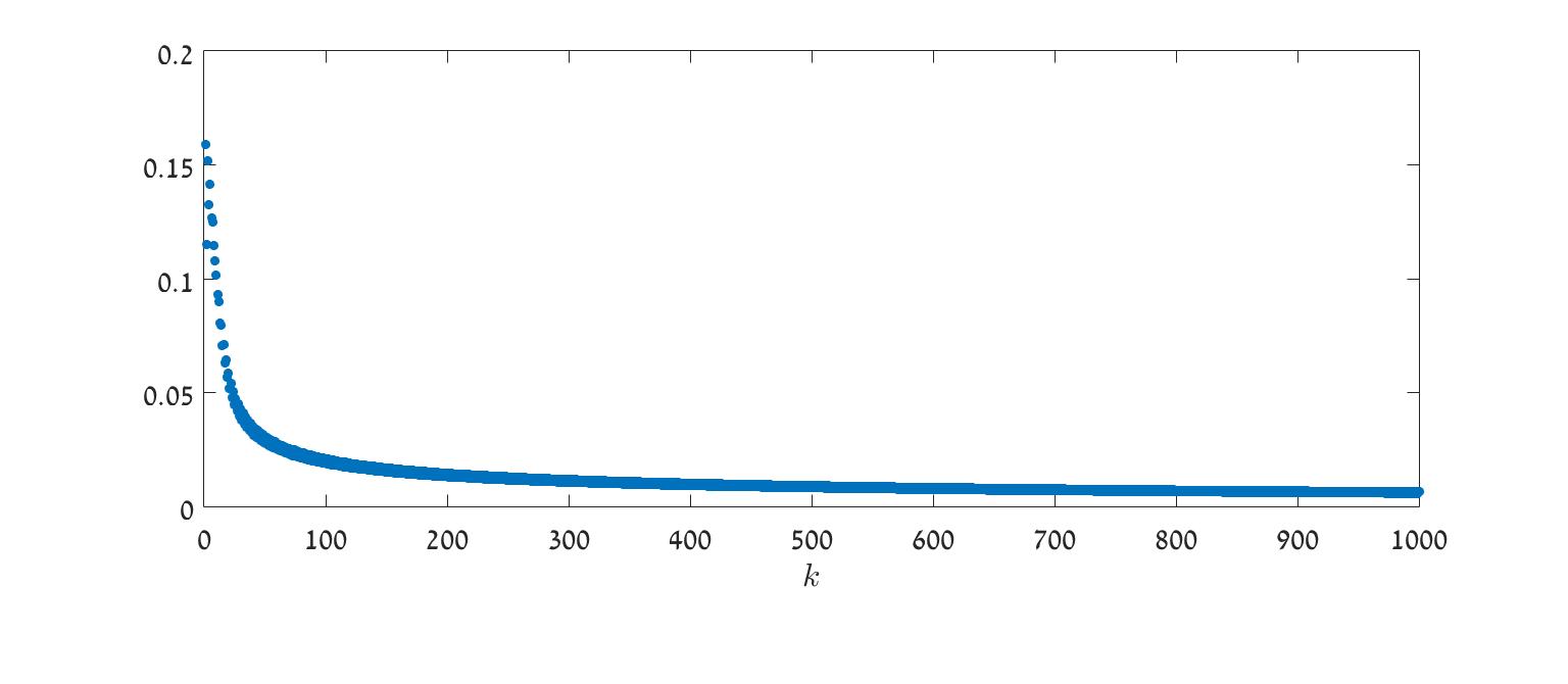
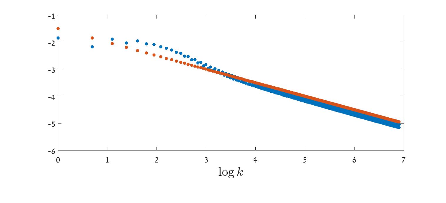
Figure 3: A plot of Erk(π2,12,[1:1])\text{Er}_{k}\left(\frac{\pi}{2},\frac{1}{2},[1:1]\right) as a function of k𝑘k (top), and (bottom) a plot of logErk(π2,12,[1:1])\log\text{Er}_{k}\left(\frac{\pi}{2},\frac{1}{2},[1:1]\right) (in blue) and −1.5−0.5​log⁡(k)1.50.5𝑘-1.5-0.5\log(k) (in red) as functions of log⁡(k)𝑘\log(k). The slope of −0.50.5-0.5 is in accordance with the fact that the sub-leading term in the estimate provided by Theorem 1.6 is (in this case) of order k−0.5superscript𝑘0.5k^{-0.5}.

3 The microsupport of partial Bergman kernels

3.1 Definition and basic properties

The notion of microsupport of an admissible sequence of holomorphic sections is specified in [4], as follows. Let (sk)k∈ℕsubscriptsubscript𝑠𝑘𝑘ℕ(s_{k})_{k\in\mathbb{N}} denote a sequence such that sk∈ℋksubscript𝑠𝑘subscriptℋ𝑘s_{k}\in\mathcal{H}_{k}. We say that (sk)k∈ℕsubscriptsubscript𝑠𝑘𝑘ℕ(s_{k})_{k\in\mathbb{N}} is admissible if there exists N>0𝑁0N>0 such that ‖sk‖=𝒪​(kN)normsubscript𝑠𝑘𝒪superscript𝑘𝑁\|s_{k}\|=\mathcal{O}(k^{N}). An admissible sequence (sk)k∈ℕsubscriptsubscript𝑠𝑘𝑘ℕ(s_{k})_{k\in\mathbb{N}} is called negligible at z0∈Msubscript𝑧0𝑀z_{0}\in M if there exists a neighborhood V𝑉V of z0subscript𝑧0z_{0} such that supz∈V|sk​(z)|z=𝒪​(k−∞)subscriptsupremum𝑧𝑉subscriptsubscript𝑠𝑘𝑧𝑧𝒪superscript𝑘\sup_{z\in V}|s_{k}(z)|_{z}=\mathcal{O}(k^{-\infty}), where |⋅|z|\cdot|_{z} is the norm on Lz⊗ksubscriptsuperscript𝐿tensor-productabsent𝑘𝑧L^{\otimes k}_{z} induced by the Hermitian product.

Definition 3.1.

The microsupport of an admissible sequence (sk)k∈ℕsubscriptsubscript𝑠𝑘𝑘ℕ(s_{k})_{k\in\mathbb{N}} is the set MS⁡(sk)⊂MMSsubscript𝑠𝑘𝑀\operatorname{MS}(s_{k})\subset M specified by

MS⁡(sk)=M∖{z∈M|(sk)k∈ℕ​ is negligible at ​z}.MSsubscript𝑠𝑘𝑀conditional-set𝑧𝑀subscriptsubscript𝑠𝑘𝑘ℕ is negligible at 𝑧\operatorname{MS}(s_{k})=M\setminus\{z\in M\ |\ (s_{k})_{k\in\mathbb{N}}\text{ is negligible at }z\}.

The notion of microsupport is also applicable to sequences (Tk)k∈ℕsubscriptsubscript𝑇𝑘𝑘ℕ(T_{k})_{k\in\mathbb{N}} with Tk∈End⁡(ℋk)subscript𝑇𝑘Endsubscriptℋ𝑘T_{k}\in\operatorname{End}(\mathcal{H}_{k}). To this end, equip M×M𝑀𝑀M\times M with the symplectic form π1∗​ω−π2∗​ωsuperscriptsubscript𝜋1𝜔superscriptsubscript𝜋2𝜔\pi_{1}^{*}\omega-\pi_{2}^{*}\omega, where π1,π2subscript𝜋1subscript𝜋2\pi_{1},\pi_{2} are the natural projections on the left and right factors. Then MS⁡(Tk)⊂M×MMSsubscript𝑇𝑘𝑀𝑀\operatorname{MS}(T_{k})\subset M\times M is defined to be the microsupport of the sequence of Schwartz kernels of Tksubscript𝑇𝑘T_{k}, which are holomorphic sections of L⊗k⊠(L∗)⊗k→M×M→⊠superscript𝐿tensor-productabsent𝑘superscriptsuperscript𝐿tensor-productabsent𝑘𝑀𝑀L^{\otimes k}\boxtimes(L^{*})^{\otimes k}\to M\times M.

Example 3.2.

([4]) Assume that Tk=Πk​ℳGk​Πksubscript𝑇𝑘subscriptΠ𝑘subscriptℳsubscript𝐺𝑘subscriptΠ𝑘T_{k}=\Pi_{k}\mathcal{M}_{G_{k}}\Pi_{k}, where Gk∈C∞​(M)subscript𝐺𝑘superscript𝐶𝑀G_{k}\in C^{\infty}(M) admits the expansion Gk=∑l=0∞gl​k−lsubscript𝐺𝑘superscriptsubscript𝑙0subscript𝑔𝑙superscript𝑘𝑙G_{k}=\sum_{l=0}^{\infty}g_{l}k^{-l} in the C∞superscript𝐶C^{\infty} topology. Then MS⁡(Tk)⊂ΔMMSsubscript𝑇𝑘subscriptΔ𝑀\operatorname{MS}(T_{k})\subset\Delta_{M}, where ΔM⊂M×MsubscriptΔ𝑀𝑀𝑀\Delta_{M}\subset M\times M is the diagonal. Viewed as a subset of M𝑀M,

MS⁡(Tk)=∪l≥0supp⁡(gl)¯.MSsubscript𝑇𝑘¯subscript𝑙0suppsubscript𝑔𝑙\operatorname{MS}(T_{k})=\overline{\cup_{l\geq 0}\operatorname{supp}(g_{l})}. (4)

3.2 Proof of Theorem 1.2

The operator F^ksubscript^𝐹𝑘\hat{F}_{k} admits the representation ([25], [16], Proposition 8.1.3)

F^k=Πk​ℳF−12​k​Δ​F​Πk,subscript^𝐹𝑘subscriptΠ𝑘subscriptℳ𝐹12𝑘Δ𝐹subscriptΠ𝑘\hat{F}_{k}=\Pi_{k}\mathcal{M}_{F-\frac{1}{2k}\Delta F}\Pi_{k}, (5)

where ΔΔ\Delta is the Laplacian defined by the Kähler metric of M𝑀M.

Lemma 3.3.

Let ε>0𝜀0\varepsilon>0. Let ψε:ℝ→[0,1]:subscript𝜓𝜀→ℝ01\psi_{\varepsilon}:\mathbb{R}\to[0,1] be a smooth function such that ψε​(t)=0subscript𝜓𝜀𝑡0\psi_{\varepsilon}(t)=0 for all t≤E−ε𝑡𝐸𝜀t\leq E-\varepsilon, ψε​(t)=1subscript𝜓𝜀𝑡1\psi_{\varepsilon}(t)=1 for all t≥E𝑡𝐸t\geq E. Write Ψ^k,ε=ψε​(Fk^)subscript^Ψ𝑘𝜀subscript𝜓𝜀^subscript𝐹𝑘\hat{\Psi}_{k,\varepsilon}=\psi_{\varepsilon}\big{(}\hat{F_{k}}\big{)}. Then MS⁡(Ψ^k,ε)⊂{F≥E−ε}MSsubscript^Ψ𝑘𝜀𝐹𝐸𝜀\operatorname{MS}(\hat{\Psi}_{k,\varepsilon})\subset\{F\geq E-\varepsilon\}.

Proof.

There exists ([4], Proposition 12) Ψk,ε∈C∞​(M)subscriptΨ𝑘𝜀superscript𝐶𝑀\Psi_{k,\varepsilon}\in C^{\infty}(M), admitting an expansion

Ψk,ε=∑l=0∞k−l​ψl,εsubscriptΨ𝑘𝜀superscriptsubscript𝑙0superscript𝑘𝑙subscript𝜓𝑙𝜀\Psi_{k,\varepsilon}=\sum_{l=0}^{\infty}k^{-l}\psi_{l,\varepsilon}

in the C∞superscript𝐶C^{\infty} topology, such that ψε​(F^k)=Πk​ℳΨk,ε​Πk+𝒪​(k−∞)subscript𝜓𝜀subscript^𝐹𝑘subscriptΠ𝑘subscriptℳsubscriptΨ𝑘𝜀subscriptΠ𝑘𝒪superscript𝑘\psi_{\varepsilon}(\hat{F}_{k})=\Pi_{k}\mathcal{M}_{\Psi_{k,\varepsilon}}\Pi_{k}+\mathcal{O}(k^{-\infty}). If F​(z)<E−ε𝐹𝑧𝐸𝜀F(z)<E-\varepsilon, then ψεsubscript𝜓𝜀\psi_{\varepsilon} vanishes in a neighborhood of F​(z)𝐹𝑧F(z), hence (using [4], p27) there exists a neighborhood V𝑉V of z𝑧z such that ψl,ε|V≡0evaluated-atsubscript𝜓𝑙𝜀𝑉0\psi_{l,\varepsilon}\big{|}_{V}\equiv 0 for all l≥0𝑙0l\geq 0. Thus, in light of (4), z∉MS⁡(ψε​(F^k))𝑧MSsubscript𝜓𝜀subscript^𝐹𝑘z\not\in\operatorname{MS}\big{(}\psi_{\varepsilon}(\hat{F}_{k})\big{)}. ∎

The first item of Theorem 1.2 now readily follows.

Corollary 3.4.

The microsupport of 𝟙[E,∞)​(F^k)subscript1𝐸subscript^𝐹𝑘\mathbbm{1}_{[E,\infty)}(\hat{F}_{k}) satisfies

MS⁡(𝟙[E,∞)​(F^k))⊂{F≥E}×{F≥E}.MSsubscript1𝐸subscript^𝐹𝑘𝐹𝐸𝐹𝐸\operatorname{MS}(\mathbbm{1}_{[E,\infty)}(\hat{F}_{k}))\subset\{F\geq E\}\times\{F\geq E\}.

The same holds for 𝟙(E,∞)​(F^k)subscript1𝐸subscript^𝐹𝑘\mathbbm{1}_{(E,\infty)}(\hat{F}_{k}).

Proof.

We prove for Ak=𝟙[E,∞)​(F^k)subscript𝐴𝑘subscript1𝐸subscript^𝐹𝑘A_{k}=\mathbbm{1}_{[E,\infty)}(\hat{F}_{k}), but the proof for 𝟙(E,∞)​(F^k)subscript1𝐸subscript^𝐹𝑘\mathbbm{1}_{(E,\infty)}(\hat{F}_{k}) is identical. Let ψεsubscript𝜓𝜀\psi_{\varepsilon} be as in Lemma 3.3, and write Ψ^k,ε=ψε​(F^k)subscript^Ψ𝑘𝜀subscript𝜓𝜀subscript^𝐹𝑘\hat{\Psi}_{k,\varepsilon}=\psi_{\varepsilon}(\hat{F}_{k}). Then

Ak=Ψ^k,ε​Ak=Ak​Ψ^k,ε,subscript𝐴𝑘subscript^Ψ𝑘𝜀subscript𝐴𝑘subscript𝐴𝑘subscript^Ψ𝑘𝜀A_{k}=\hat{\Psi}_{k,\varepsilon}A_{k}=A_{k}\hat{\Psi}_{k,\varepsilon},

hence (using [4], p24)

MS⁡(Ak)=MS⁡(Ψ^k,ε​Ak)MSsubscript𝐴𝑘MSsubscript^Ψ𝑘𝜀subscript𝐴𝑘\displaystyle\operatorname{MS}(A_{k})=\operatorname{MS}(\hat{\Psi}_{k,\varepsilon}A_{k})
⊂{(z1,z3)|∃z2∈M​such that ​(z1,z2)∈MS⁡(Ψ^k,ε)​ and ​(z2,z3)∈MS⁡(Ak)}absentconditional-setsubscript𝑧1subscript𝑧3subscript𝑧2𝑀such that subscript𝑧1subscript𝑧2MSsubscript^Ψ𝑘𝜀 and subscript𝑧2subscript𝑧3MSsubscript𝐴𝑘\displaystyle\subset\{(z_{1},z_{3})\ |\ \exists z_{2}\in M\ \text{such that }(z_{1},z_{2})\in\operatorname{MS}(\hat{\Psi}_{k,\varepsilon})\text{ and }(z_{2},z_{3})\in\operatorname{MS}(A_{k})\}
⊂MS⁡(Ψ^k,ε)×M,absentMSsubscript^Ψ𝑘𝜀𝑀\displaystyle\subset\operatorname{MS}(\hat{\Psi}_{k,\varepsilon})\times M,

where by a slight abuse of notation, in the second line MS⁡(Ψ^k,ε)MSsubscript^Ψ𝑘𝜀\operatorname{MS}(\hat{\Psi}_{k,\varepsilon}) is viewed as a subset of M×M𝑀𝑀M\times M, and in the third line it is viewed as a subset of M𝑀M. Repeating this argument,

MS⁡(Ak)=MS⁡(Ak​Ψ^k,ε)⊂M×MS⁡(Ψ^k,ε),MSsubscript𝐴𝑘MSsubscript𝐴𝑘subscript^Ψ𝑘𝜀𝑀MSsubscript^Ψ𝑘𝜀\operatorname{MS}(A_{k})=\operatorname{MS}(A_{k}\hat{\Psi}_{k,\varepsilon})\subset M\times\operatorname{MS}(\hat{\Psi}_{k,\varepsilon}),

therefore (noting Lemma 3.3)

MS⁡(Ak)⊂(MS⁡(Ψ^k,ε)×M)∩(M×MS⁡(Ψ^k,ε))MSsubscript𝐴𝑘MSsubscript^Ψ𝑘𝜀𝑀𝑀MSsubscript^Ψ𝑘𝜀\displaystyle\operatorname{MS}(A_{k})\subset\left(\operatorname{MS}(\hat{\Psi}_{k,\varepsilon})\times M\right)\cap\left(M\times\operatorname{MS}(\hat{\Psi}_{k,\varepsilon})\right)
=MS⁡(Ψ^k,ε)×MS⁡(Ψ^k,ε)⊂{F≥E−ε}×{F≥E−ε}.absentMSsubscript^Ψ𝑘𝜀MSsubscript^Ψ𝑘𝜀𝐹𝐸𝜀𝐹𝐸𝜀\displaystyle=\operatorname{MS}(\hat{\Psi}_{k,\varepsilon})\times\operatorname{MS}(\hat{\Psi}_{k,\varepsilon})\subset\{F\geq E-\varepsilon\}\times\{F\geq E-\varepsilon\}.

Since ε>0𝜀0\varepsilon>0 is arbitrary, we obtain the required. ∎

The second item of Theorem 1.2 immediately follows from Corollary 3.4.

Corollary 3.5.

Replacing F𝐹F with G=−F𝐺𝐹G=-F and E𝐸E with −E𝐸-E, if G​(z)<−E𝐺𝑧𝐸G(z)<-E or G​(w)<−E𝐺𝑤𝐸G(w)<-E then there exists a neighborhood 𝒩⊂M×M𝒩𝑀𝑀\mathcal{N}\subset M\times M of (z,w)𝑧𝑤(z,w) such that

sup𝒩|𝟙(−E,∞)​(G^k)|=𝒪​(k−∞),subscriptsupremum𝒩subscript1𝐸subscript^𝐺𝑘𝒪superscript𝑘\sup_{\mathcal{N}}\left|\mathbbm{1}_{(-E,\infty)}(\hat{G}_{k})\right|=\mathcal{O}(k^{-\infty}),

where

𝟙(−E,∞)​(G^k)=Πk−𝟙(−∞,−E]​(G^k)=Πk−𝟙[E,∞)​(F^k),subscript1𝐸subscript^𝐺𝑘subscriptΠ𝑘subscript1𝐸subscript^𝐺𝑘subscriptΠ𝑘subscript1𝐸subscript^𝐹𝑘\displaystyle\mathbbm{1}_{(-E,\infty)}(\hat{G}_{k})=\Pi_{k}-\mathbbm{1}_{(-\infty,-E]}(\hat{G}_{k})=\Pi_{k}-\mathbbm{1}_{[E,\infty)}(\hat{F}_{k}),

that is, sup𝒩|Πk−𝟙[E,∞)​(F^k)|=𝒪​(k−∞)subscriptsupremum𝒩subscriptΠ𝑘subscript1𝐸subscript^𝐹𝑘𝒪superscript𝑘\sup_{\mathcal{N}}\left|\Pi_{k}-\mathbbm{1}_{[E,\infty)}(\hat{F}_{k})\right|=\mathcal{O}(k^{-\infty}).

Finally,

Lemma 3.6.

Corollary 3.4 implies Corollary 1.5.

Proof.

We keep the notations used in the formulation of Corollary 1.5, and also write

Πk,1=𝟙[E1,∞)​(F^k),Πk,2=𝟙[E2,∞)​(G^k).formulae-sequencesubscriptΠ𝑘1subscript1subscript𝐸1subscript^𝐹𝑘subscriptΠ𝑘2subscript1subscript𝐸2subscript^𝐺𝑘\Pi_{k,1}=\mathbbm{1}_{[E_{1},\infty)}(\hat{F}_{k}),\ \Pi_{k,2}=\mathbbm{1}_{[E_{2},\infty)}(\hat{G}_{k}).

Then using Corollary 3.4,

MS⁡(Πk,1​Πk,2)MSsubscriptΠ𝑘1subscriptΠ𝑘2\displaystyle\operatorname{MS}\left(\Pi_{k,1}\Pi_{k,2}\right)
⊂{(z1,z3)|∃z2∈M​ such that ​(z1,z2)∈MS⁡(Πk,1)​ and ​(z2,z3)∈MS⁡(Πk,2)}absentconditional-setsubscript𝑧1subscript𝑧3subscript𝑧2𝑀 such that subscript𝑧1subscript𝑧2MSsubscriptΠ𝑘1 and subscript𝑧2subscript𝑧3MSsubscriptΠ𝑘2\displaystyle\subset\{(z_{1},z_{3})\ |\ \exists z_{2}\in M\text{ such that }(z_{1},z_{2})\in\operatorname{MS}(\Pi_{k,1})\text{ and }(z_{2},z_{3})\in\operatorname{MS}\left(\Pi_{k,2}\right)\}
⊂{(z1,z3)|∃z2∈M​ such that ​z2∈{F≥E1}∩{G≥E2}}=∅.absentconditional-setsubscript𝑧1subscript𝑧3subscript𝑧2𝑀 such that subscript𝑧2𝐹subscript𝐸1𝐺subscript𝐸2\displaystyle\subset\{(z_{1},z_{3})\ |\ \exists z_{2}\in M\text{ such that }z_{2}\in\{F\geq E_{1}\}\cap\{G\geq E_{2}\}\}=\emptyset.

Thus Πk,1​Πk,2subscriptΠ𝑘1subscriptΠ𝑘2\Pi_{k,1}\Pi_{k,2} is a negligible sequence, which implies ([4], Remark 5) that ‖Πk,1​Πk,2‖op=𝒪​(k−∞)subscriptnormsubscriptΠ𝑘1subscriptΠ𝑘2op𝒪superscript𝑘\|\Pi_{k,1}\Pi_{k,2}\|_{\operatorname{op}}=\mathcal{O}(k^{-\infty}).∎

The proof of the first part of the first item of Theorem 1.7 is essentially identical to that of Theorem 1.2. Namely,

Lemma 3.7.

Let λksubscript𝜆𝑘\lambda_{k} be a sequence of eigenvalues of F^ksubscript^𝐹𝑘\hat{F}_{k} with |λk−E|=𝒪​(k−1)subscript𝜆𝑘𝐸𝒪superscript𝑘1|\lambda_{k}-E|=\mathcal{O}(k^{-1}), where E∈F​(M)𝐸𝐹𝑀E\in F(M). Let Πk,λk,FsubscriptΠ𝑘subscript𝜆𝑘𝐹\Pi_{k,\lambda_{k},F} be the orthogonal projection onto the eigenspace associated with λksubscript𝜆𝑘\lambda_{k}. Then MS⁡(Πk,λk,F)⊂{F=E}×{F=E}MSsubscriptΠ𝑘subscript𝜆𝑘𝐹𝐹𝐸𝐹𝐸\operatorname{MS}(\Pi_{k,\lambda_{k},F})\subset\{F=E\}\times\{F=E\}.

Proof.

Given ε>0𝜀0\varepsilon>0 we consider a smooth function ψε:ℝ→[0,1]:subscript𝜓𝜀→ℝ01\psi_{\varepsilon}:\mathbb{R}\to[0,1] such that ψε​(t)=1subscript𝜓𝜀𝑡1\psi_{\varepsilon}(t)=1 whenever |t−E|<ε2𝑡𝐸𝜀2|t-E|<\frac{\varepsilon}{2} and ψε​(t)=0subscript𝜓𝜀𝑡0\psi_{\varepsilon}(t)=0 whenever |t−E|≥ε𝑡𝐸𝜀|t-E|\geq\varepsilon. Write Ψ^k,ε=ψε​(F^k)subscript^Ψ𝑘𝜀subscript𝜓𝜀subscript^𝐹𝑘\hat{\Psi}_{k,\varepsilon}=\psi_{\varepsilon}(\hat{F}_{k}), and note that exactly as in Lemma 3.3,

MS⁡(Ψ^k,ε)⊂{|F−E|≤ε}×{|F−E|≤ε}.MSsubscript^Ψ𝑘𝜀𝐹𝐸𝜀𝐹𝐸𝜀\operatorname{MS}(\hat{\Psi}_{k,\varepsilon})\subset\{|F-E|\leq\varepsilon\}\times\{|F-E|\leq\varepsilon\}.

For every sufficiently large k𝑘k, it holds that Ψ^k,ε​Πk,λk,F=Πk,λk,F​Ψ^k,ε=Πk,λk,Fsubscript^Ψ𝑘𝜀subscriptΠ𝑘subscript𝜆𝑘𝐹subscriptΠ𝑘subscript𝜆𝑘𝐹subscript^Ψ𝑘𝜀subscriptΠ𝑘subscript𝜆𝑘𝐹\hat{\Psi}_{k,\varepsilon}\Pi_{k,\lambda_{k},F}=\Pi_{k,\lambda_{k},F}\hat{\Psi}_{k,\varepsilon}=\Pi_{k,\lambda_{k},F}. Thus, exactly as in Corollary 3.4, we obtain that

MS⁡(Πk,λk,F)⊂MS⁡(Ψ^k,ε)×MS⁡(ψε​(F^k))⊂{|F−E|≤ε}×{|F−E|≤ε}.MSsubscriptΠ𝑘subscript𝜆𝑘𝐹MSsubscript^Ψ𝑘𝜀MSsubscript𝜓𝜀subscript^𝐹𝑘𝐹𝐸𝜀𝐹𝐸𝜀\operatorname{MS}(\Pi_{k,\lambda_{k},F})\subset\operatorname{MS}(\hat{\Psi}_{k,\varepsilon})\times\operatorname{MS}(\psi_{\varepsilon}(\hat{F}_{k}))\subset\{|F-E|\leq\varepsilon\}\times\{|F-E|\leq\varepsilon\}.

Since ε𝜀\varepsilon is arbitrary, MS⁡(Πk,λk)⊂{F=E}×{F=E}MSsubscriptΠ𝑘subscript𝜆𝑘𝐹𝐸𝐹𝐸\operatorname{MS}(\Pi_{k,\lambda_{k}})\subset\{F=E\}\times\{F=E\}. ∎

4 Fourier theory and partial Bergman kernels

4.1 The Cauchy-Szegö projection on the circle

Let ℝ/2​π​ℤ=S1⊂ℂℝ2𝜋ℤsuperscript𝑆1ℂ\mathbb{R}/2\pi\mathbb{Z}=S^{1}\subset\mathbb{C} denote the unit circle. Let g^​(p)=⟨g,ep⟩L2​(S1)^𝑔𝑝subscript𝑔subscript𝑒𝑝superscript𝐿2superscript𝑆1\hat{g}(p)=\langle g,e_{p}\rangle_{L^{2}(S^{1})} denote the p𝑝p-th Fourier coefficient of g∈L1​(S1)𝑔superscript𝐿1superscript𝑆1g\in L^{1}(S^{1}), where p∈ℤ𝑝ℤp\in\mathbb{Z} and ep​(t)=ei​p​tsubscript𝑒𝑝𝑡superscript𝑒𝑖𝑝𝑡e_{p}(t)=e^{ipt}. The Cauchy-Szegö projection ΠS1:L2​(S1)→H2​(S1):subscriptΠsuperscript𝑆1→superscript𝐿2superscript𝑆1superscript𝐻2superscript𝑆1\Pi_{S^{1}}:L^{2}(S^{1})\to H^{2}(S^{1}) is the orthogonal projection on the Hardy space

H2​(S1)={g∈L2​(S1)|g^​(p)=0​∀p<0},superscript𝐻2superscript𝑆1conditional-set𝑔superscript𝐿2superscript𝑆1^𝑔𝑝0for-all𝑝0H^{2}(S^{1})=\left\{g\in L^{2}(S^{1})\ |\ \hat{g}(p)=0\ \forall p<0\right\},

and it admits the formula

ΠS1​(g)​(t)=limr→1−12​π​∫−ππg​(t−s)1−r​ei​s​𝑑s.subscriptΠsuperscript𝑆1𝑔𝑡subscript→𝑟superscript112𝜋superscriptsubscript𝜋𝜋𝑔𝑡𝑠1𝑟superscript𝑒𝑖𝑠differential-d𝑠\Pi_{S^{1}}(g)(t)=\lim_{r\to 1^{-}}\frac{1}{2\pi}\int_{-\pi}^{\pi}\frac{g(t-s)}{1-re^{is}}ds.

The periodic Hilbert transform ℋS1:L2​(S1)→L2​(S1):subscriptℋsuperscript𝑆1→superscript𝐿2superscript𝑆1superscript𝐿2superscript𝑆1\mathcal{H}_{S^{1}}:L^{2}(S^{1})\to L^{2}(S^{1}) is specified by ℋS1​(ep)=−i​sgn⁡(p)​epsubscriptℋsuperscript𝑆1subscript𝑒𝑝𝑖sgn𝑝subscript𝑒𝑝\mathcal{H}_{S^{1}}(e_{p})=-i\operatorname{sgn}(p)e_{p}, or equivalently

ℋS1​(g)​(t)=limε→0+12​π​∫ε≤|t−s|≤πg​(s)​cot⁡(t−s2)​𝑑s.subscriptℋsuperscript𝑆1𝑔𝑡subscript→𝜀superscript012𝜋subscript𝜀𝑡𝑠𝜋𝑔𝑠𝑡𝑠2differential-d𝑠\mathcal{H}_{S^{1}}(g)(t)=\lim_{\varepsilon\to 0^{+}}\frac{1}{2\pi}\int_{\varepsilon\leq|t-s|\leq\pi}g(s)\cot\left(\frac{t-s}{2}\right)ds.
Corollary 4.1.

The Cauchy-Szegö projection acts by ep​(t)↦𝟙[0,∞)​(p)​ep​(t)maps-tosubscript𝑒𝑝𝑡subscript10𝑝subscript𝑒𝑝𝑡e_{p}(t)\mapsto\mathbbm{1}_{[0,\infty)}(p)e_{p}(t), hence it can be expressed in terms of the periodic Hilbert transform, as follows:

ΠS1​(g)=12​(i​ℋS1​(g)+g+g^​(0)).subscriptΠsuperscript𝑆1𝑔12𝑖subscriptℋsuperscript𝑆1𝑔𝑔^𝑔0\Pi_{S^{1}}(g)=\frac{1}{2}\left(i\mathcal{H}_{S^{1}}(g)+g+\hat{g}(0)\right).

4.2 Spectral projections and unitary representations of S1superscript𝑆1S^{1}

Let ℋℋ\mathcal{H} denote a finite dimensional complex Hilbert space, and write dimℋ=ddimensionℋ𝑑\dim\mathcal{H}=d. Let A∈End⁡(ℋ)𝐴EndℋA\in\operatorname{End}(\mathcal{H}) be a Hermitian operator. Denote

UA​(t)=ei​t​A,subscript𝑈𝐴𝑡superscript𝑒𝑖𝑡𝐴U_{A}(t)=e^{itA},

and assume that t↦UA​(t)maps-to𝑡subscript𝑈𝐴𝑡t\mapsto U_{A}(t) is 2​π2𝜋2\pi-periodic.

Let v1,…,vdsubscript𝑣1…subscript𝑣𝑑v_{1},...,v_{d} be an orthonormal eigenbasis of A𝐴A such that A​vm=pm​vm𝐴subscript𝑣𝑚subscript𝑝𝑚subscript𝑣𝑚Av_{m}=p_{m}v_{m}, with p1≤p2≤…≤pdsubscript𝑝1subscript𝑝2…subscript𝑝𝑑p_{1}\leq p_{2}\leq...\leq p_{d}. Then pm∈ℤsubscript𝑝𝑚ℤp_{m}\in\mathbb{Z}, and we can write

A=∑m=1dpm​vm⊗vm∗,UA​(t)=∑m=1dei​t​pm​vm⊗vm∗,formulae-sequence𝐴superscriptsubscript𝑚1𝑑tensor-productsubscript𝑝𝑚subscript𝑣𝑚superscriptsubscript𝑣𝑚subscript𝑈𝐴𝑡superscriptsubscript𝑚1𝑑tensor-productsuperscript𝑒𝑖𝑡subscript𝑝𝑚subscript𝑣𝑚superscriptsubscript𝑣𝑚A=\sum_{m=1}^{d}p_{m}v_{m}\otimes v_{m}^{*},\ U_{A}(t)=\sum_{m=1}^{d}e^{itp_{m}}v_{m}\otimes v_{m}^{*},

where vm∗superscriptsubscript𝑣𝑚v_{m}^{*} is the dual vector of vmsubscript𝑣𝑚v_{m}.

Corollary 4.2.

The spectral projection ΠA=𝟙[0,∞)​(A)subscriptΠ𝐴subscript10𝐴\Pi_{A}=\mathbbm{1}_{[0,\infty)}(A) can be written in the following form:

ΠA=(ΠS1​(UA))​(0)=limr→1−12​π​∫−ππUA​(s)1−r​ei​s​𝑑s.subscriptΠ𝐴subscriptΠsuperscript𝑆1subscript𝑈𝐴0subscript→𝑟superscript112𝜋superscriptsubscript𝜋𝜋subscript𝑈𝐴𝑠1𝑟superscript𝑒𝑖𝑠differential-d𝑠\Pi_{A}=\left(\Pi_{S^{1}}(U_{A})\right)(0)=\lim_{r\to 1^{-}}\frac{1}{2\pi}\int_{-\pi}^{\pi}\frac{U_{A}(s)}{1-re^{is}}ds.

In terms of the Hilbert transform,

ΠA=12​(i​ℋS1​(UA)​(0)+Idℋ+U^A​(0)),subscriptΠ𝐴12𝑖subscriptℋsuperscript𝑆1subscript𝑈𝐴0subscriptIdℋsubscript^𝑈𝐴0\Pi_{A}=\frac{1}{2}\left(i\mathcal{H}_{S^{1}}(U_{A})(0)+\operatorname{Id}_{\mathcal{H}}+\widehat{U}_{A}(0)\right), (6)

where

U^A​(0)=12​π​∫−ππUA​(t)​𝑑tsubscript^𝑈𝐴012𝜋superscriptsubscript𝜋𝜋subscript𝑈𝐴𝑡differential-d𝑡\widehat{U}_{A}(0)=\frac{1}{2\pi}\int_{-\pi}^{\pi}U_{A}(t)dt

and

ℋS1​(UA)​(0)=12​π​∫0π(UA​(−t)−UA​(t))​cot⁡(t2)​𝑑t.subscriptℋsuperscript𝑆1subscript𝑈𝐴012𝜋superscriptsubscript0𝜋subscript𝑈𝐴𝑡subscript𝑈𝐴𝑡𝑡2differential-d𝑡\mathcal{H}_{S^{1}}(U_{A})(0)=\frac{1}{2\pi}\int_{0}^{\pi}\left(U_{A}(-t)-U_{A}(t)\right)\cot\left(\frac{t}{2}\right)dt.

More generally, given p,p0∈ℤ𝑝subscript𝑝0ℤp,p_{0}\in\mathbb{Z} and g∈L2​(S1)𝑔superscript𝐿2superscript𝑆1g\in L^{2}(S^{1}), recall that

e−p0​g^​(p)=⟨e−p0​g,ep⟩L2​(S1)=⟨g,ep+p0⟩L2​(S1)=g^​(p+p0).^subscript𝑒subscript𝑝0𝑔𝑝subscriptsubscript𝑒subscript𝑝0𝑔subscript𝑒𝑝superscript𝐿2superscript𝑆1subscript𝑔subscript𝑒𝑝subscript𝑝0superscript𝐿2superscript𝑆1^𝑔𝑝subscript𝑝0\widehat{e_{-p_{0}}g}(p)=\langle e_{-p_{0}}g,e_{p}\rangle_{L^{2}(S^{1})}=\langle g,e_{p+p_{0}}\rangle_{L^{2}(S^{1})}=\hat{g}(p+p_{0}).

This relation allows us to extend formula (6) to ΠA,E=𝟙[E,∞)​(A)subscriptΠ𝐴𝐸subscript1𝐸𝐴\Pi_{A,E}=\mathbbm{1}_{[E,\infty)}(A), E∈ℝ𝐸ℝE\in\mathbb{R}.

Corollary 4.3.

Let E∈ℝ𝐸ℝE\in\mathbb{R}. Denote UA,E=e−⌈E⌉​UAsubscript𝑈𝐴𝐸subscript𝑒𝐸subscript𝑈𝐴U_{A,E}=e_{-\lceil E\rceil}U_{A}. Then

ΠA,E=(ΠS1​(UA,E))​(0)=12​(i​ℋS1​(UA,E)​(0)+Idℋ+U^A,E​(0)),subscriptΠ𝐴𝐸subscriptΠsuperscript𝑆1subscript𝑈𝐴𝐸012𝑖subscriptℋsuperscript𝑆1subscript𝑈𝐴𝐸0subscriptIdℋsubscript^𝑈𝐴𝐸0\Pi_{A,E}=\left(\Pi_{S^{1}}(U_{A,E})\right)(0)=\frac{1}{2}\left(i\mathcal{H}_{S^{1}}(U_{A,E})(0)+\operatorname{Id}_{\mathcal{H}}+\widehat{U}_{A,E}(0)\right), (7)

where

U^A,E​(0)=12​π​∫−ππUA,E​(t)​𝑑t=12​π​∫−ππUA​(t)​e−i​⌈E⌉​t​𝑑tsubscript^𝑈𝐴𝐸012𝜋superscriptsubscript𝜋𝜋subscript𝑈𝐴𝐸𝑡differential-d𝑡12𝜋superscriptsubscript𝜋𝜋subscript𝑈𝐴𝑡superscript𝑒𝑖𝐸𝑡differential-d𝑡\widehat{U}_{A,E}(0)=\frac{1}{2\pi}\int_{-\pi}^{\pi}U_{A,E}(t)dt=\frac{1}{2\pi}\int_{-\pi}^{\pi}U_{A}(t)e^{-i\lceil E\rceil t}dt

and

ℋS1​(UA,E)​(0)=12​π​∫0π(UA​(−t)​ei​⌈E⌉​t−UA​(t)​e−i​⌈E⌉​t)​cot⁡(t2)​𝑑t.subscriptℋsuperscript𝑆1subscript𝑈𝐴𝐸012𝜋superscriptsubscript0𝜋subscript𝑈𝐴𝑡superscript𝑒𝑖𝐸𝑡subscript𝑈𝐴𝑡superscript𝑒𝑖𝐸𝑡𝑡2differential-d𝑡\mathcal{H}_{S^{1}}(U_{A,E})(0)=\frac{1}{2\pi}\int_{0}^{\pi}\left(U_{A}(-t)e^{i\lceil E\rceil t}-U_{A}(t)e^{-i\lceil E\rceil t}\right)\cot\left(\frac{t}{2}\right)dt.

4.3 Proof of Theorems 1.6, 1.7

The proof of Theorem 1.6 relies on formula (7), which is also applicable to the Schwartz kernels of the operators involved. Thus, we obtain a representation of Πk,E​(z,w)subscriptΠ𝑘𝐸𝑧𝑤\Pi_{k,E}(z,w) in terms of the Bergman kernel and the Schwartz kernel of the quantum propagator defined by H^ksubscript^𝐻𝑘\hat{H}_{k}. The well-known asymptotic properties of the Bergman kernel, with the help of the stationary phase lemma, produce the desired estimate. Notably, we can assume without loss of generality that the circle action is effective (Lemma 4.4), and then the third term in (7) is the equivariant Bergman projection associated with the eigenvalue ⌈k​E⌉k𝑘𝐸𝑘\frac{\lceil kE\rceil}{k} of H^ksubscript^𝐻𝑘\hat{H}_{k}. Accordingly, the proof of Theorem 1.6 relies on the second item of Theorem 1.7. The latter is established by similar arguments, namely, the stationary phase lemma is used together with the integral representation of equivariant Bergman kernels as ”Fourier coefficients” of the full Bergman kernel.

Recall that there exists N≥1𝑁1N\geq 1 and an open dense subset MN⊂Msubscript𝑀𝑁𝑀M_{N}\subset M such that the stabilizer group of every z∈MN𝑧subscript𝑀𝑁z\in M_{N} is the subgroup SN1⊂S1subscriptsuperscript𝑆1𝑁superscript𝑆1S^{1}_{N}\subset S^{1} of order N𝑁N. We assume throughout that N=1𝑁1N=1 (i.e., that the circle action is effective); this is justified by the following lemma.

Lemma 4.4.

It suffices to prove Theorems 1.6, 1.7 in the case N=1𝑁1N=1.

Proof.

Assume that N>1𝑁1N>1. If t∈SN1𝑡subscriptsuperscript𝑆1𝑁t\in S^{1}_{N}, then φt|MN=Idevaluated-atsubscript𝜑𝑡subscript𝑀𝑁Id\varphi_{t}|_{M_{N}}=\operatorname{Id}, hence by continuity φt=Idsubscript𝜑𝑡Id\varphi_{t}=\operatorname{Id}. It follows that t↦φN,t=φtNmaps-to𝑡subscript𝜑𝑁𝑡subscript𝜑𝑡𝑁t\mapsto\varphi_{N,t}=\varphi_{\frac{t}{N}}, t∈ℝ/2​π​ℤ𝑡ℝ2𝜋ℤt\in\mathbb{R}/2\pi\mathbb{Z}, is an effective holomorphic circle action, generated by the Hamiltonian HN=1N​Hsubscript𝐻𝑁1𝑁𝐻H_{N}=\frac{1}{N}H. Writing H^N,k=1N​H^ksubscript^𝐻𝑁𝑘1𝑁subscript^𝐻𝑘\hat{H}_{N,k}=\frac{1}{N}\hat{H}_{k},

Πk,E=𝟙[E,∞)​(H^k)=𝟙[EN,∞)​(H^N,k).subscriptΠ𝑘𝐸subscript1𝐸subscript^𝐻𝑘subscript1𝐸𝑁subscript^𝐻𝑁𝑘\Pi_{k,E}=\mathbbm{1}_{[E,\infty)}(\hat{H}_{k})=\mathbbm{1}_{[\frac{E}{N},\infty)}\left(\hat{H}_{N,k}\right).

Thus, the case N>1𝑁1N>1 is reduced to the case N=1𝑁1N=1. Similarly,

Πk,λkeq=𝟙{λk}​(H^k)=𝟙{λkN}​(H^N,k).subscriptsuperscriptΠeq𝑘subscript𝜆𝑘subscript1subscript𝜆𝑘subscript^𝐻𝑘subscript1subscript𝜆𝑘𝑁subscript^𝐻𝑁𝑘\Pi^{\operatorname{eq}}_{k,\lambda_{k}}=\mathbbm{1}_{\{\lambda_{k}\}}(\hat{H}_{k})=\mathbbm{1}_{\{\frac{\lambda_{k}}{N}\}}(\hat{H}_{N,k}).

∎

Recall that E∈H​(M)𝐸𝐻𝑀E\in H(M) is a regular value of H𝐻H, and assume that z∈H−1​(E)𝑧superscript𝐻1𝐸z\in H^{-1}(E). Denote Vk​(t)=ei​k​t​H^ksubscript𝑉𝑘𝑡superscript𝑒𝑖𝑘𝑡subscript^𝐻𝑘V_{k}(t)=e^{ikt\hat{H}_{k}}, and consider the map

Vk​(z,w):S1→Lz⊗k⊗(Lw∗)⊗k:subscript𝑉𝑘𝑧𝑤→superscript𝑆1tensor-productsuperscriptsubscript𝐿𝑧tensor-productabsent𝑘superscriptsuperscriptsubscript𝐿𝑤tensor-productabsent𝑘V_{k}(z,w):S^{1}\to L_{z}^{\otimes k}\otimes(L_{w}^{*})^{\otimes k}

specified by t↦Vk​(t)​(z,w)maps-to𝑡subscript𝑉𝑘𝑡𝑧𝑤t\mapsto V_{k}(t)(z,w), where the latter is the Schwartz kernel of Vk​(t)subscript𝑉𝑘𝑡V_{k}(t). Denote Ek=⌈k​E⌉ksubscript𝐸𝑘𝑘𝐸𝑘E_{k}=\frac{\lceil kE\rceil}{k} and Vk,Ek​(t)​(z,w)=e−i​k​Ek​t​Vk​(t)​(z,w)subscript𝑉𝑘subscript𝐸𝑘𝑡𝑧𝑤superscript𝑒𝑖𝑘subscript𝐸𝑘𝑡subscript𝑉𝑘𝑡𝑧𝑤V_{k,E_{k}}(t)(z,w)=e^{-ikE_{k}t}V_{k}(t)(z,w). According to (7),

Πk,E​(z,w)=12​(i​ℋS1​(Vk,Ek​(z,w))​(0)+Πk​(z,w)+Vk,Ek​(z,w)^​(0)),subscriptΠ𝑘𝐸𝑧𝑤12𝑖subscriptℋsuperscript𝑆1subscript𝑉𝑘subscript𝐸𝑘𝑧𝑤0subscriptΠ𝑘𝑧𝑤^subscript𝑉𝑘subscript𝐸𝑘𝑧𝑤0\Pi_{k,E}(z,w)=\frac{1}{2}\left(i\mathcal{H}_{S^{1}}\left(V_{k,E_{k}}(z,w)\right)(0)+\Pi_{k}(z,w)+\widehat{V_{k,E_{k}}(z,w)}(0)\right), (8)

where

Vk,Ek​(z,w)^​(0)=12​π​∫02​πVk,Ek​(t)​(z,w)​𝑑t=Πk,Ekeq​(z,w)^subscript𝑉𝑘subscript𝐸𝑘𝑧𝑤012𝜋superscriptsubscript02𝜋subscript𝑉𝑘subscript𝐸𝑘𝑡𝑧𝑤differential-d𝑡subscriptsuperscriptΠeq𝑘subscript𝐸𝑘𝑧𝑤\widehat{V_{k,E_{k}}(z,w)}(0)=\frac{1}{2\pi}\int_{0}^{2\pi}V_{k,E_{k}}(t)(z,w)dt=\Pi^{\operatorname{eq}}_{k,E_{k}}(z,w)

is the equivariant Bergman kernel associated with the eigenvalue Eksubscript𝐸𝑘E_{k} of H^ksubscript^𝐻𝑘\hat{H}_{k}. The Schwartz kernel of Vk,Ek​(t)subscript𝑉𝑘subscript𝐸𝑘𝑡V_{k,E_{k}}(t) admits the following useful formula.

Lemma 4.5.

The Schwartz kernel of Vk,Ek​(t)subscript𝑉𝑘subscript𝐸𝑘𝑡V_{k,E_{k}}(t) is specified by

Vk,Ek​(t)​(z,w)=ck,Ek​(z,t)​𝒯k,t​(Πk​(φt​(z),w)),subscript𝑉𝑘subscript𝐸𝑘𝑡𝑧𝑤subscript𝑐𝑘subscript𝐸𝑘𝑧𝑡subscript𝒯𝑘𝑡subscriptΠ𝑘subscript𝜑𝑡𝑧𝑤V_{k,E_{k}}(t)(z,w)=c_{k,E_{k}}(z,t)\mathcal{T}_{k,t}\left(\Pi_{k}(\varphi_{t}(z),w)\right),

where 𝒯k,t:Lφt​(z)⊗k⊗(L∗)w⊗k→Lz⊗k⊗(L∗)w⊗k:subscript𝒯𝑘𝑡→tensor-productsubscriptsuperscript𝐿tensor-productabsent𝑘subscript𝜑𝑡𝑧subscriptsuperscriptsuperscript𝐿tensor-productabsent𝑘𝑤tensor-productsubscriptsuperscript𝐿tensor-productabsent𝑘𝑧subscriptsuperscriptsuperscript𝐿tensor-productabsent𝑘𝑤\mathcal{T}_{k,t}:L^{\otimes k}_{\varphi_{t}(z)}\otimes(L^{*})^{\otimes k}_{w}\to L^{\otimes k}_{z}\otimes(L^{*})^{\otimes k}_{w} is the parallel transport along the curve t′↦(φt−t′​(z),w)maps-tosuperscript𝑡′subscript𝜑𝑡superscript𝑡′𝑧𝑤t^{\prime}\mapsto\left(\varphi_{t-t^{\prime}}(z),w\right), t′∈[0,t]superscript𝑡′0𝑡t^{\prime}\in[0,t], and ck,Ek​(z,t)=ei​k​(H​(z)−Ek)​t=ei​k​(E−Ek)​tsubscript𝑐𝑘subscript𝐸𝑘𝑧𝑡superscript𝑒𝑖𝑘𝐻𝑧subscript𝐸𝑘𝑡superscript𝑒𝑖𝑘𝐸subscript𝐸𝑘𝑡c_{k,E_{k}}(z,t)=e^{ik(H(z)-E_{k})t}=e^{ik(E-E_{k})t}.

Proof.

As shown in [16], Proposition 8.2.1, the action of Vk​(t)subscript𝑉𝑘𝑡V_{k}(t) is specified by

Vk​(t)​s​(z)=ei​k​t​H​(z)​τk,t​s​(φt​(z)),s∈ℋk,formulae-sequencesubscript𝑉𝑘𝑡𝑠𝑧superscript𝑒𝑖𝑘𝑡𝐻𝑧subscript𝜏𝑘𝑡𝑠subscript𝜑𝑡𝑧𝑠subscriptℋ𝑘V_{k}(t)s(z)=e^{iktH(z)}\tau_{k,t}s(\varphi_{t}(z)),\ s\in\mathcal{H}_{k},

where τk,t:Lφt​(z)⊗k→Lz⊗k:subscript𝜏𝑘𝑡→subscriptsuperscript𝐿tensor-productabsent𝑘subscript𝜑𝑡𝑧subscriptsuperscript𝐿tensor-productabsent𝑘𝑧\tau_{k,t}:L^{\otimes k}_{\varphi_{t}(z)}\to L^{\otimes k}_{z} is the parallel transport along the curve t′↦φt−t′​(z)maps-tosuperscript𝑡′subscript𝜑𝑡superscript𝑡′𝑧t^{\prime}\mapsto\varphi_{t-t^{\prime}}(z), t′∈[0,t]superscript𝑡′0𝑡t^{\prime}\in[0,t]. Thus, considering any orthonormal basis s1,…,sdksubscript𝑠1…subscript𝑠subscript𝑑𝑘s_{1},...,s_{d_{k}} of ℋksubscriptℋ𝑘\mathcal{H}_{k}, we find that the Schwartz kernel of Vk​(t)subscript𝑉𝑘𝑡V_{k}(t) is given by

Vk​(t)​(z,w)subscript𝑉𝑘𝑡𝑧𝑤\displaystyle V_{k}(t)(z,w) =∑m=1dk(Vk​(t)​sm)​(z)⊗sm∗​(w)absentsuperscriptsubscript𝑚1subscript𝑑𝑘tensor-productsubscript𝑉𝑘𝑡subscript𝑠𝑚𝑧superscriptsubscript𝑠𝑚𝑤\displaystyle=\sum_{m=1}^{d_{k}}\left(V_{k}(t)s_{m}\right)(z)\otimes s_{m}^{*}(w)
=ei​k​t​H​(z)​∑m=1dk(τk,t​sm)​(φt​(z))⊗sm∗​(w)absentsuperscript𝑒𝑖𝑘𝑡𝐻𝑧superscriptsubscript𝑚1subscript𝑑𝑘tensor-productsubscript𝜏𝑘𝑡subscript𝑠𝑚subscript𝜑𝑡𝑧superscriptsubscript𝑠𝑚𝑤\displaystyle=e^{iktH(z)}\sum_{m=1}^{d_{k}}\left(\tau_{k,t}s_{m}\right)(\varphi_{t}(z))\otimes s_{m}^{*}(w)
=ei​k​t​H​(z)​(τk,t⊗Id)​(∑m=1dksm​(φt​(z))⊗sm∗​(w))absentsuperscript𝑒𝑖𝑘𝑡𝐻𝑧tensor-productsubscript𝜏𝑘𝑡Idsuperscriptsubscript𝑚1subscript𝑑𝑘tensor-productsubscript𝑠𝑚subscript𝜑𝑡𝑧superscriptsubscript𝑠𝑚𝑤\displaystyle=e^{iktH(z)}\left(\tau_{k,t}\otimes\operatorname{Id}\right)\left(\sum_{m=1}^{d_{k}}s_{m}(\varphi_{t}(z))\otimes s_{m}^{*}(w)\right)
=ei​k​t​H​(z)​𝒯k,t​(Πk​(φt​(z),w)).absentsuperscript𝑒𝑖𝑘𝑡𝐻𝑧subscript𝒯𝑘𝑡subscriptΠ𝑘subscript𝜑𝑡𝑧𝑤\displaystyle=e^{iktH(z)}\mathcal{T}_{k,t}\left(\Pi_{k}(\varphi_{t}(z),w)\right).

Multiplying both sides by e−i​k​Ek​tsuperscript𝑒𝑖𝑘subscript𝐸𝑘𝑡e^{-ikE_{k}t}, we obtain the required. ∎

The microsupport MS⁡(Πk)MSsubscriptΠ𝑘\operatorname{MS}(\Pi_{k}) of ΠksubscriptΠ𝑘\Pi_{k} equals the diagonal ΔM⊂M×MsubscriptΔ𝑀𝑀𝑀\Delta_{M}\subset M\times M. In particular, this implies (see [4], Proposition 8, or [19], Theorem 1) that for every ε>0𝜀0\varepsilon>0 and N>0𝑁0N>0 there exists Cε,N>0subscript𝐶𝜀𝑁0C_{\varepsilon,N}>0 such that for every z,w∈M𝑧𝑤𝑀z,w\in M, if dist⁡(z,w)≥εdist𝑧𝑤𝜀\operatorname{dist}(z,w)\geq\varepsilon then

|Πk​(z,w)|<Cε,N​k−N,subscriptΠ𝑘𝑧𝑤subscript𝐶𝜀𝑁superscript𝑘𝑁\lvert\Pi_{k}(z,w)\rvert<C_{\varepsilon,N}k^{-N}, (9)

and that for every vector field Y𝑌Y on M×M𝑀𝑀M\times M there exists CY,ε,Nsubscript𝐶𝑌𝜀𝑁C_{Y,\varepsilon,N} such that for every z,w∈M𝑧𝑤𝑀z,w\in M, if dist⁡(z,w)≥εdist𝑧𝑤𝜀\operatorname{dist}(z,w)\geq\varepsilon then

|(∇~k)Y​Πk​(z,w)|<CY,ε,N​k−N.subscriptsubscript~∇𝑘𝑌subscriptΠ𝑘𝑧𝑤subscript𝐶𝑌𝜀𝑁superscript𝑘𝑁\lvert(\tilde{\nabla}_{k})_{Y}\Pi_{k}(z,w)\rvert<C_{Y,\varepsilon,N}k^{-N}. (10)

Here, ∇~ksubscript~∇𝑘\tilde{\nabla}_{k} is the connection on L⊗k⊠(L∗)⊗k⊠superscript𝐿tensor-productabsent𝑘superscriptsuperscript𝐿tensor-productabsent𝑘L^{\otimes k}\boxtimes(L^{*})^{\otimes k} induced by ∇∇\nabla. The first part of Theorem 1.6 readily follows from these estimates.

Lemma 4.6.

If z∈M𝑧𝑀z\in M and w∈M∖𝒪z𝑤𝑀subscript𝒪𝑧w\in M\setminus\mathcal{O}_{z}, then (z,w)∉MS⁡(Πk,E)𝑧𝑤MSsubscriptΠ𝑘𝐸(z,w)\not\in\operatorname{MS}(\Pi_{k,E}).

Proof.

Let 𝒩0⊂M×Msubscript𝒩0𝑀𝑀\mathcal{N}_{0}\subset M\times M denote a neighborhood of (z,w)𝑧𝑤(z,w) such that for every (z′,w′)∈𝒩0superscript𝑧′superscript𝑤′subscript𝒩0(z^{\prime},w^{\prime})\in\mathcal{N}_{0} and t∈[−π,π]𝑡𝜋𝜋t\in[-\pi,\pi],

dist⁡(φt​(z′),w′)>ε2distsubscript𝜑𝑡superscript𝑧′superscript𝑤′𝜀2\operatorname{dist}(\varphi_{t}(z^{\prime}),w^{\prime})>\frac{\varepsilon}{2}

for some ε>0𝜀0\varepsilon>0. We wish to prove that

sup𝒩0|Πk,E|=𝒪​(k−∞),subscriptsupremumsubscript𝒩0subscriptΠ𝑘𝐸𝒪superscript𝑘\sup_{\mathcal{N}_{0}}\lvert\Pi_{k,E}\rvert=\mathcal{O}(k^{-\infty}),

which would mean (by definition) that (z,w)∉MS⁡(Πk,E)𝑧𝑤MSsubscriptΠ𝑘𝐸(z,w)\not\in\operatorname{MS}(\Pi_{k,E}). Let

𝒩={(φt​(z′),w′)|(z′,w′)∈𝒩0,t∈[−π,π]}.𝒩conditional-setsubscript𝜑𝑡superscript𝑧′superscript𝑤′formulae-sequencesuperscript𝑧′superscript𝑤′subscript𝒩0𝑡𝜋𝜋\mathcal{N}=\{(\varphi_{t}(z^{\prime}),w^{\prime})\ |\ (z^{\prime},w^{\prime})\in\mathcal{N}_{0},\ t\in[-\pi,\pi]\}.

Looking at the representation (8) in light of (9), we immediately note that the second term satisfies

sup𝒩0|Πk|=𝒪​(k−∞).subscriptsupremumsubscript𝒩0subscriptΠ𝑘𝒪superscript𝑘\sup_{\mathcal{N}_{0}}|\Pi_{k}|=\mathcal{O}(k^{-\infty}).

Similarly, estimate (9) implies that the term Vk,Ek​(z′,w′)^​(0)=Πk,Ekeq​(z′,w′)^subscript𝑉𝑘subscript𝐸𝑘superscript𝑧′superscript𝑤′0subscriptsuperscriptΠeq𝑘subscript𝐸𝑘superscript𝑧′superscript𝑤′\widehat{V_{k,E_{k}}(z^{\prime},w^{\prime})}(0)=\Pi^{\operatorname{eq}}_{k,E_{k}}(z^{\prime},w^{\prime}), which is the equivariant Bergman kernel associated with the eigenvalue Eksubscript𝐸𝑘E_{k}, satisfies

sup(z′,w′)∈𝒩0|Πk,Ekeq​(z′,w′)|≤sup𝒩012​π​∫−ππ|Πk​(φt​(z′),w′)|​𝑑t=𝒪​(k−∞).subscriptsupremumsuperscript𝑧′superscript𝑤′subscript𝒩0subscriptsuperscriptΠeq𝑘subscript𝐸𝑘superscript𝑧′superscript𝑤′subscriptsupremumsubscript𝒩012𝜋superscriptsubscript𝜋𝜋subscriptΠ𝑘subscript𝜑𝑡superscript𝑧′superscript𝑤′differential-d𝑡𝒪superscript𝑘\sup_{(z^{\prime},w^{\prime})\in\mathcal{N}_{0}}\left|\Pi^{\operatorname{eq}}_{k,E_{k}}(z^{\prime},w^{\prime})\right|\leq\sup_{\mathcal{N}_{0}}\frac{1}{2\pi}\int_{-\pi}^{\pi}\left|\Pi_{k}\left(\varphi_{t}(z^{\prime}),w^{\prime}\right)\right|dt=\mathcal{O}(k^{-\infty}). (11)

Finally, consider the first term in (8). Let Vk,Ek′​(u)​(z′,w′)=dd​t​(Vk​(z′,w′))​(u)subscriptsuperscript𝑉′𝑘subscript𝐸𝑘𝑢superscript𝑧′superscript𝑤′𝑑𝑑𝑡subscript𝑉𝑘superscript𝑧′superscript𝑤′𝑢V^{\prime}_{k,E_{k}}(u)(z^{\prime},w^{\prime})=\frac{d}{dt}\big{(}V_{k}(z^{\prime},w^{\prime})\big{)}(u). Note that Vk,Ek​(0)​(z′,w′)=Πk​(z′,w′)subscript𝑉𝑘subscript𝐸𝑘0superscript𝑧′superscript𝑤′subscriptΠ𝑘superscript𝑧′superscript𝑤′V_{k,E_{k}}(0)(z^{\prime},w^{\prime})=\Pi_{k}(z^{\prime},w^{\prime}). If t∈(0,π)𝑡0𝜋t\in(0,\pi), then by the mean-value theorem,

|Vk,Ek​(t)​(z′,w′)−Πk​(z′,w′)|≤t​supu∈[0,t]|Vk,Ek′​(u)​(z′,w′)|,subscript𝑉𝑘subscript𝐸𝑘𝑡superscript𝑧′superscript𝑤′subscriptΠ𝑘superscript𝑧′superscript𝑤′𝑡subscriptsupremum𝑢0𝑡superscriptsubscript𝑉𝑘subscript𝐸𝑘′𝑢superscript𝑧′superscript𝑤′|V_{k,E_{k}}(t)(z^{\prime},w^{\prime})-\Pi_{k}(z^{\prime},w^{\prime})|\leq t\sup_{u\in[0,t]}\left|V_{k,E_{k}}^{\prime}(u)(z^{\prime},w^{\prime})\right|,

where (in light of Lemma 4.5)

Vk,Ek′​(u)​(z′,w′)=ck,Ek​(u)​𝒯k,u​(i​k​(E−Ek)​Πk​(φu​(z′),w′)+(∇~k)YH​(Πk)​(φu​(z′),w′)),subscriptsuperscript𝑉′𝑘subscript𝐸𝑘𝑢superscript𝑧′superscript𝑤′subscript𝑐𝑘subscript𝐸𝑘𝑢subscript𝒯𝑘𝑢𝑖𝑘𝐸subscript𝐸𝑘subscriptΠ𝑘subscript𝜑𝑢superscript𝑧′superscript𝑤′subscriptsubscript~∇𝑘subscript𝑌𝐻subscriptΠ𝑘subscript𝜑𝑢superscript𝑧′superscript𝑤′V^{\prime}_{k,E_{k}}(u)(z^{\prime},w^{\prime})=\\ c_{k,E_{k}}(u)\mathcal{T}_{k,u}\left(ik(E-E_{k})\Pi_{k}(\varphi_{u}(z^{\prime}),w^{\prime})+(\tilde{\nabla}_{k})_{Y_{H}}(\Pi_{k})(\varphi_{u}(z^{\prime}),w^{\prime})\right),

with YH=(XH,0)subscript𝑌𝐻subscript𝑋𝐻0Y_{H}=(X_{H},0).

Applying (9) and (10), we see that

|Vk,Ek′​(u)​(z′,w′)|subscriptsuperscript𝑉′𝑘subscript𝐸𝑘𝑢superscript𝑧′superscript𝑤′\displaystyle\left|V^{\prime}_{k,E_{k}}(u)(z^{\prime},w^{\prime})\right| ≤k​|E−Ek|​|Πk​(φu​(z′),w′)|+|(∇~k)YH​Πk​(φu​(z′),w′)|absent𝑘𝐸subscript𝐸𝑘subscriptΠ𝑘subscript𝜑𝑢superscript𝑧′superscript𝑤′subscriptsubscript~∇𝑘subscript𝑌𝐻subscriptΠ𝑘subscript𝜑𝑢superscript𝑧′superscript𝑤′\displaystyle\leq k|E-E_{k}||\Pi_{k}(\varphi_{u}(z^{\prime}),w^{\prime})|+|(\tilde{\nabla}_{k})_{Y_{H}}\Pi_{k}(\varphi_{u}(z^{\prime}),w^{\prime})| (12)
≤sup𝒩|Πk|+sup𝒩|(∇~k)YH​Πk|=𝒪​(k−∞).absentsubscriptsupremum𝒩subscriptΠ𝑘subscriptsupremum𝒩subscriptsubscript~∇𝑘subscript𝑌𝐻subscriptΠ𝑘𝒪superscript𝑘\displaystyle\leq\sup_{\mathcal{N}}|\Pi_{k}|+\sup_{\mathcal{N}}|(\tilde{\nabla}_{k})_{Y_{H}}\Pi_{k}|=\mathcal{O}(k^{-\infty}).

Thus,

sup𝒩0×(0,π)1t​|Vk,Ek​(t)​(z′,w′)−Πk​(z′,w′)|=𝒪​(k−∞),subscriptsupremumsubscript𝒩00𝜋1𝑡subscript𝑉𝑘subscript𝐸𝑘𝑡superscript𝑧′superscript𝑤′subscriptΠ𝑘superscript𝑧′superscript𝑤′𝒪superscript𝑘\sup_{\mathcal{N}_{0}\times(0,\pi)}\frac{1}{t}\left|V_{k,E_{k}}(t)(z^{\prime},w^{\prime})-\Pi_{k}(z^{\prime},w^{\prime})\right|=\mathcal{O}(k^{-\infty}),

which implies (since if t≈0𝑡0t\approx 0, then cot⁡(t2)≈2t𝑡22𝑡\cot\left(\frac{t}{2}\right)\approx\frac{2}{t}) that

sup𝒩0|ℋS1​(Vk,Ek​(z′,w′))​(0)|=𝒪​(k−∞).subscriptsupremumsubscript𝒩0subscriptℋsuperscript𝑆1subscript𝑉𝑘subscript𝐸𝑘superscript𝑧′superscript𝑤′0𝒪superscript𝑘\sup_{\mathcal{N}_{0}}\left|\mathcal{H}_{S^{1}}(V_{k,E_{k}}(z^{\prime},w^{\prime}))(0)\right|=\mathcal{O}(k^{-\infty}).

∎

We proceed with the proof of the second item of Theorem 1.6, relying on formula (8). Fix a,b∈ℝ𝑎𝑏ℝa,b\in\mathbb{R}. The behaviour of the third term in (8) is specified in Theorem 1.7, hence in what follows we focus on ℋS1​(Vk,Ek​(zak,0,zbk,t0))​(0)subscriptℋsuperscript𝑆1subscript𝑉𝑘subscript𝐸𝑘subscript𝑧subscript𝑎𝑘0subscript𝑧subscript𝑏𝑘subscript𝑡00\mathcal{H}_{S^{1}}\left(V_{k,E_{k}}(z_{a_{k},0},z_{b_{k},t_{0}})\right)(0), where we denote ak=aksubscript𝑎𝑘𝑎𝑘a_{k}=\frac{a}{\sqrt{k}}, bk=bksubscript𝑏𝑘𝑏𝑘b_{k}=\frac{b}{\sqrt{k}}, and for any α∈ℝ𝛼ℝ\alpha\in\mathbb{R}, t∈S1𝑡superscript𝑆1t\in S^{1},

zα=ψα​(z0),zα,t=φt​(zα).formulae-sequencesubscript𝑧𝛼subscript𝜓𝛼subscript𝑧0subscript𝑧𝛼𝑡subscript𝜑𝑡subscript𝑧𝛼z_{\alpha}=\psi_{\alpha}(z_{0}),\ z_{\alpha,t}=\varphi_{t}(z_{\alpha}).
Lemma 4.7.

Fix z0∈H−1​(E)∩M1subscript𝑧0superscript𝐻1𝐸subscript𝑀1z_{0}\in H^{-1}(E)\cap M_{1}. Let ℐ⊂S1∖{0}ℐsuperscript𝑆10\mathcal{I}\subset S^{1}\setminus\{0\} be a closed interval. Then for every fixed δ>0𝛿0\delta>0 small enough, if t0∈ℐsubscript𝑡0ℐt_{0}\in\mathcal{I} then

ℋS1​(Vk,Ek​(zak,zbk,t0))​(0)=subscriptℋsuperscript𝑆1subscript𝑉𝑘subscript𝐸𝑘subscript𝑧subscript𝑎𝑘subscript𝑧subscript𝑏𝑘subscript𝑡00absent\displaystyle\mathcal{H}_{S^{1}}(V_{k,E_{k}}(z_{a_{k}},z_{b_{k},t_{0}}))(0)=
−12​π​∫t0−δt0+δVk,Ek​(t)​(zak,zbk,t0)​cot⁡(t2)​𝑑t+rk​(a,b,t0).12𝜋superscriptsubscriptsubscript𝑡0𝛿subscript𝑡0𝛿subscript𝑉𝑘subscript𝐸𝑘𝑡subscript𝑧subscript𝑎𝑘subscript𝑧subscript𝑏𝑘subscript𝑡0𝑡2differential-d𝑡subscript𝑟𝑘𝑎𝑏subscript𝑡0\displaystyle-\frac{1}{2\pi}\int_{t_{0}-\delta}^{t_{0}+\delta}V_{k,E_{k}}(t)(z_{a_{k}},z_{b_{k},t_{0}})\cot\left(\frac{t}{2}\right)dt+r_{k}(a,b,t_{0}).

Here, rk​(a,b,t0)=𝒪​(k−∞)subscript𝑟𝑘𝑎𝑏subscript𝑡0𝒪superscript𝑘r_{k}(a,b,t_{0})=\mathcal{O}(k^{-\infty}) uniformly, in the following sense: for every bounded set B⊂ℝ𝐵ℝB\subset\mathbb{R} and N>0𝑁0N>0, there exists cB,N>0subscript𝑐𝐵𝑁0c_{B,N}>0 such that |rk​(a,b,t0)|≤cB,N​k−Nsubscript𝑟𝑘𝑎𝑏subscript𝑡0subscript𝑐𝐵𝑁superscript𝑘𝑁|r_{k}(a,b,t_{0})|\leq c_{B,N}k^{-N} for every a,b∈B𝑎𝑏𝐵a,b\in B, t0∈ℐsubscript𝑡0ℐt_{0}\in\mathcal{I}.

Proof.

Assume that ℐ=[t′,t′′]⊂(0,2​π)ℐsuperscript𝑡′superscript𝑡′′02𝜋\mathcal{I}=[t^{\prime},t^{\prime\prime}]\subset(0,2\pi). Let δ>0𝛿0\delta>0 be small enough so that

([0,δ]∪[2​π−δ,2​π])∩[t′−δ,t′′+δ]=∅.0𝛿2𝜋𝛿2𝜋superscript𝑡′𝛿superscript𝑡′′𝛿\left([0,\delta]\cup[2\pi-\delta,2\pi]\right)\cap[t^{\prime}-\delta,t^{\prime\prime}+\delta]=\emptyset.

There exists ε>0𝜀0\varepsilon>0 such that for every t∈[0,2​π]𝑡02𝜋t\in[0,2\pi] and t0∈ℐsubscript𝑡0ℐt_{0}\in\mathcal{I}, if |t−t0|≥δ𝑡subscript𝑡0𝛿|t-t_{0}|\geq\delta then dist⁡(z0,t,z0,t0)>εdistsubscript𝑧0𝑡subscript𝑧0subscript𝑡0𝜀\operatorname{dist}(z_{0,t},z_{0,t_{0}})>\varepsilon. Let B⊂ℝ𝐵ℝB\subset\mathbb{R} be bounded. There exists k0∈ℕsubscript𝑘0ℕk_{0}\in\mathbb{N} such that for every k≥k0𝑘subscript𝑘0k\geq k_{0}, for every a,b∈B𝑎𝑏𝐵a,b\in B and for every t∈[0,2​π]𝑡02𝜋t\in[0,2\pi], t0∈ℐsubscript𝑡0ℐt_{0}\in\mathcal{I} such that |t−t0|≥δ𝑡subscript𝑡0𝛿|t-t_{0}|\geq\delta, it holds that

dist⁡(zak,t,zbk,t0)>ε2.distsubscript𝑧subscript𝑎𝑘𝑡subscript𝑧subscript𝑏𝑘subscript𝑡0𝜀2\operatorname{dist}(z_{a_{k},t},z_{b_{k},t_{0}})>\frac{\varepsilon}{2}. (13)

Thus, the mean-value theorem together with a suitable version of estimate (12) imply that

sup(0,δ]|(Vk,Ek​(t)​(zak,zbk,t0)−Vk,Ek​(−t)​(zak,zbk,t0))​cot⁡(t2)|=𝒪​(k−∞),subscriptsupremum0𝛿subscript𝑉𝑘subscript𝐸𝑘𝑡subscript𝑧subscript𝑎𝑘subscript𝑧subscript𝑏𝑘subscript𝑡0subscript𝑉𝑘subscript𝐸𝑘𝑡subscript𝑧subscript𝑎𝑘subscript𝑧subscript𝑏𝑘subscript𝑡0𝑡2𝒪superscript𝑘\sup_{(0,\delta]}\left|\left(V_{k,E_{k}}(t)(z_{a_{k}},z_{b_{k},t_{0}})-V_{k,E_{k}}(-t)(z_{a_{k}},z_{b_{k},t_{0}})\right)\cot\left(\frac{t}{2}\right)\right|=\mathcal{O}(k^{-\infty}),

and (in light of (13), (10)) the estimate is uniform for a,b∈B𝑎𝑏𝐵a,b\in B and t0∈ℐsubscript𝑡0ℐt_{0}\in\mathcal{I}. Thus,

∫0π(Vk,Ek​(t)​(zak,zbk,t0)−Vk,Ek​(−t)​(zak,zbk,t0))​cot⁡(t2)​𝑑t=∫δπ(Vk,Ek​(t)​(zak,zbk,t0)−Vk,Ek​(−t)​(zak,zbk,t0))​cot⁡(t2)​𝑑t+𝒪​(k−∞)=∫δ2​π−δVk,Ek​(t)​(zak,zbk,t0)​cot⁡(t2)​𝑑t+𝒪​(k−∞),superscriptsubscript0𝜋subscript𝑉𝑘subscript𝐸𝑘𝑡subscript𝑧subscript𝑎𝑘subscript𝑧subscript𝑏𝑘subscript𝑡0subscript𝑉𝑘subscript𝐸𝑘𝑡subscript𝑧subscript𝑎𝑘subscript𝑧subscript𝑏𝑘subscript𝑡0𝑡2differential-d𝑡superscriptsubscript𝛿𝜋subscript𝑉𝑘subscript𝐸𝑘𝑡subscript𝑧subscript𝑎𝑘subscript𝑧subscript𝑏𝑘subscript𝑡0subscript𝑉𝑘subscript𝐸𝑘𝑡subscript𝑧subscript𝑎𝑘subscript𝑧subscript𝑏𝑘subscript𝑡0𝑡2differential-d𝑡𝒪superscript𝑘superscriptsubscript𝛿2𝜋𝛿subscript𝑉𝑘subscript𝐸𝑘𝑡subscript𝑧subscript𝑎𝑘subscript𝑧subscript𝑏𝑘subscript𝑡0𝑡2differential-d𝑡𝒪superscript𝑘\int_{0}^{\pi}\left(V_{k,E_{k}}(t)(z_{a_{k}},z_{b_{k},t_{0}})-V_{k,E_{k}}(-t)(z_{a_{k}},z_{b_{k},t_{0}})\right)\cot\left(\frac{t}{2}\right)dt=\\ \int_{\delta}^{\pi}\left(V_{k,E_{k}}(t)(z_{a_{k}},z_{b_{k},t_{0}})-V_{k,E_{k}}(-t)(z_{a_{k}},z_{b_{k},t_{0}})\right)\cot\left(\frac{t}{2}\right)dt+\mathcal{O}(k^{-\infty})\\ =\int_{\delta}^{2\pi-\delta}V_{k,E_{k}}(t)(z_{a_{k}},z_{b_{k},t_{0}})\cot\left(\frac{t}{2}\right)dt+\mathcal{O}(k^{-\infty}),

where (in light of (13), (9)) the remainder estimate is uniform for a,b∈B𝑎𝑏𝐵a,b\in B and t0∈ℐsubscript𝑡0ℐt_{0}\in\mathcal{I}. Finally,

∫δt0−δVk,Ek​(t)​(zak,zbk,t0)​cot⁡(t2)​𝑑t=𝒪​(k−∞),superscriptsubscript𝛿subscript𝑡0𝛿subscript𝑉𝑘subscript𝐸𝑘𝑡subscript𝑧subscript𝑎𝑘subscript𝑧subscript𝑏𝑘subscript𝑡0𝑡2differential-d𝑡𝒪superscript𝑘\int_{\delta}^{t_{0}-\delta}V_{k,E_{k}}(t)(z_{a_{k}},z_{b_{k},t_{0}})\cot\left(\frac{t}{2}\right)dt=\mathcal{O}(k^{-\infty}),

and again, by (13), (9), the estimate is uniform for a,b∈B𝑎𝑏𝐵a,b\in B, t0∈ℐsubscript𝑡0ℐt_{0}\in\mathcal{I}. Similarly for the integration over [t0+δ,2​π−δ]subscript𝑡0𝛿2𝜋𝛿[t_{0}+\delta,2\pi-\delta]. ∎

Corollary 4.8.

Let Sk​(z,w)=σ​(z)⊗k⊗(σinv∗​(w))⊗ksubscript𝑆𝑘𝑧𝑤tensor-product𝜎superscript𝑧tensor-productabsent𝑘superscriptsubscriptsuperscript𝜎inv𝑤tensor-productabsent𝑘S_{k}(z,w)=\sigma(z)^{\otimes k}\otimes(\sigma^{*}_{\operatorname{inv}}(w))^{\otimes k}, where σ=sinv|sinv|𝜎subscript𝑠invsubscript𝑠inv\sigma=\frac{s_{\operatorname{inv}}}{|s_{\operatorname{inv}}|}, with sinvsubscript𝑠invs_{\operatorname{inv}} a local non-vanishing invariant section of L𝐿L in a neighborhood of 𝒪z0subscript𝒪subscript𝑧0\mathcal{O}_{z_{0}}. Note that ‖XH‖normsubscript𝑋𝐻\|X_{H}\| is constant in 𝒪z0subscript𝒪subscript𝑧0\mathcal{O}_{z_{0}}. In light of the previous lemma and (17), we conclude that

−(2​πk)n​ℋS1​(Vk,Ek​(zak,zbk,t0))​(0)=superscript2𝜋𝑘𝑛subscriptℋsuperscript𝑆1subscript𝑉𝑘subscript𝐸𝑘subscript𝑧subscript𝑎𝑘subscript𝑧subscript𝑏𝑘subscript𝑡00absent\displaystyle-\left(\frac{2\pi}{k}\right)^{n}\mathcal{H}_{S^{1}}(V_{k,E_{k}}(z_{a_{k}},z_{b_{k},t_{0}}))(0)=
(e−(a2+b2)2​‖XH​(z0)‖2​e−i​k​Ek​t0​cot⁡(t02)‖XH​(z0)‖​π​k+Ck​(a,b,t0))​Sk​(zak,zbk,t0).superscript𝑒superscript𝑎2superscript𝑏22superscriptnormsubscript𝑋𝐻subscript𝑧02superscript𝑒𝑖𝑘subscript𝐸𝑘subscript𝑡0subscript𝑡02normsubscript𝑋𝐻subscript𝑧0𝜋𝑘subscript𝐶𝑘𝑎𝑏subscript𝑡0subscript𝑆𝑘subscript𝑧subscript𝑎𝑘subscript𝑧subscript𝑏𝑘subscript𝑡0\displaystyle\left(e^{-\frac{(a^{2}+b^{2})}{2}\|X_{H}(z_{0})\|^{2}}e^{-ikE_{k}t_{0}}\frac{\cot\left(\frac{t_{0}}{2}\right)}{\|X_{H}(z_{0})\|\sqrt{\pi k}}+C_{k}(a,b,t_{0})\right)S_{k}(z_{a_{k}},z_{b_{k},t_{0}}).

Here, Ck​(a,b,t0)=Ckv​(a,b,t0)2​πsubscript𝐶𝑘𝑎𝑏subscript𝑡0subscriptsuperscript𝐶𝑣𝑘𝑎𝑏subscript𝑡02𝜋C_{k}(a,b,t_{0})=\frac{C^{v}_{k}(a,b,t_{0})}{2\pi}, where Ckv​(a,b,t)superscriptsubscript𝐶𝑘𝑣𝑎𝑏𝑡C_{k}^{v}(a,b,t) is as specified in Corollary 5.2, with v​(t)=cot⁡(t2)𝑣𝑡𝑡2v(t)=\cot\left(\frac{t}{2}\right).

In order to complete the proof of Theorem 1.6, it remains to establish the off-diagonal estimate for the equivariant Bergman kernel Πk,EksubscriptΠ𝑘subscript𝐸𝑘\Pi_{k,E_{k}}, as formulated in Theorem 1.7. Hence, we now turn to address the proof of the latter. Assume that λksubscript𝜆𝑘\lambda_{k} is an eigenvalue of H^ksubscript^𝐻𝑘\hat{H}_{k} such that |λk−E|=𝒪​(k−1)subscript𝜆𝑘𝐸𝒪superscript𝑘1\lvert\lambda_{k}-E\rvert=\mathcal{O}(k^{-1}). Let

Πk,λkeq=12​π​∫02​πVk​(t)​e−i​k​λk​t​𝑑tsubscriptsuperscriptΠeq𝑘subscript𝜆𝑘12𝜋superscriptsubscript02𝜋subscript𝑉𝑘𝑡superscript𝑒𝑖𝑘subscript𝜆𝑘𝑡differential-d𝑡\Pi^{\operatorname{eq}}_{k,\lambda_{k}}=\frac{1}{2\pi}\int_{0}^{2\pi}V_{k}(t)e^{-ik\lambda_{k}t}dt

denote the orthogonal projection on the eigenspace associated with λksubscript𝜆𝑘\lambda_{k}.

Corollary 4.9.

Estimate (11) in the proof of Lemma 4.6 is also valid for Πk,λkeqsubscriptsuperscriptΠeq𝑘subscript𝜆𝑘\Pi^{\operatorname{eq}}_{k,\lambda_{k}}. Namely, if z∈M𝑧𝑀z\in M and w∈M∖𝒪z𝑤𝑀subscript𝒪𝑧w\in M\setminus\mathcal{O}_{z}, then (z,w)∉MS⁡(Πk,λkeq)𝑧𝑤MSsubscriptsuperscriptΠeq𝑘subscript𝜆𝑘(z,w)\not\in\operatorname{MS}(\Pi^{\operatorname{eq}}_{k,\lambda_{k}}). Together with Lemma 3.7, we obtain the first item of Theorem 1.7.

Corollary 4.10.

Let z0∈H−1​(E)∩M1subscript𝑧0superscript𝐻1𝐸subscript𝑀1z_{0}\in H^{-1}(E)\cap M_{1} and ℐ⊂S1ℐsuperscript𝑆1\mathcal{I}\subset S^{1} be a closed interval. The same argument as in the proof of Lemma 4.7 implies that for every fixed δ>0𝛿0\delta>0 small enough, if t0∈ℐsubscript𝑡0ℐt_{0}\in\mathcal{I} then

Πk,λkeq​(zak,zbk,t0)=∫t0−δt0+δVk​(t)​(zak,zbk,t0)​e−i​k​λk​t​𝑑t+rkeq​(a,b,t0).subscriptsuperscriptΠeq𝑘subscript𝜆𝑘subscript𝑧subscript𝑎𝑘subscript𝑧subscript𝑏𝑘subscript𝑡0superscriptsubscriptsubscript𝑡0𝛿subscript𝑡0𝛿subscript𝑉𝑘𝑡subscript𝑧subscript𝑎𝑘subscript𝑧subscript𝑏𝑘subscript𝑡0superscript𝑒𝑖𝑘subscript𝜆𝑘𝑡differential-d𝑡subscriptsuperscript𝑟eq𝑘𝑎𝑏subscript𝑡0\Pi^{\operatorname{eq}}_{k,\lambda_{k}}(z_{a_{k}},z_{b_{k},t_{0}})=\int_{t_{0}-\delta}^{t_{0}+\delta}V_{k}(t)(z_{a_{k}},z_{b_{k},t_{0}})e^{-ik\lambda_{k}t}dt+r^{\operatorname{eq}}_{k}(a,b,t_{0}).

Here, rkeq​(a,b,t0)=𝒪​(k−∞)subscriptsuperscript𝑟eq𝑘𝑎𝑏subscript𝑡0𝒪superscript𝑘r^{\operatorname{eq}}_{k}(a,b,t_{0})=\mathcal{O}(k^{-\infty}) uniformly, as before: for every B⊂ℝ𝐵ℝB\subset\mathbb{R} bounded and N>0𝑁0N>0, there exists cB,N>0subscript𝑐𝐵𝑁0c_{B,N}>0 such that |rkeq​(a,b,t0)|≤cB,N​k−Nsubscriptsuperscript𝑟eq𝑘𝑎𝑏subscript𝑡0subscript𝑐𝐵𝑁superscript𝑘𝑁|r^{\operatorname{eq}}_{k}(a,b,t_{0})|\leq c_{B,N}k^{-N} for every a,b∈B𝑎𝑏𝐵a,b\in B, t0∈ℐsubscript𝑡0ℐt_{0}\in\mathcal{I}.

Thus, by (17),

(2​πk)n​Πk,λkeq​(zak,zbk,t0)=superscript2𝜋𝑘𝑛subscriptsuperscriptΠeq𝑘subscript𝜆𝑘subscript𝑧subscript𝑎𝑘subscript𝑧subscript𝑏𝑘subscript𝑡0absent\displaystyle\left(\frac{2\pi}{k}\right)^{n}\Pi^{\operatorname{eq}}_{k,\lambda_{k}}(z_{a_{k}},z_{b_{k},t_{0}})=
(e−(a2+b2)2​‖XH​(z0)‖2​e−i​k​λk​t0​1‖XH​(z0)‖​π​k+Ckeq​(a,b,t0))​Sk​(zak,zbk,t0),superscript𝑒superscript𝑎2superscript𝑏22superscriptnormsubscript𝑋𝐻subscript𝑧02superscript𝑒𝑖𝑘subscript𝜆𝑘subscript𝑡01normsubscript𝑋𝐻subscript𝑧0𝜋𝑘subscriptsuperscript𝐶eq𝑘𝑎𝑏subscript𝑡0subscript𝑆𝑘subscript𝑧subscript𝑎𝑘subscript𝑧subscript𝑏𝑘subscript𝑡0\displaystyle\left(e^{-\frac{(a^{2}+b^{2})}{2}\|X_{H}(z_{0})\|^{2}}e^{-ik\lambda_{k}t_{0}}\frac{1}{\|X_{H}(z_{0})\|\sqrt{\pi k}}+C^{\operatorname{eq}}_{k}(a,b,t_{0})\right)S_{k}(z_{a_{k}},z_{b_{k},t_{0}}),

where Ckeq​(a,b,t0)=Ckv​(a,b,t0)2​πsuperscriptsubscript𝐶𝑘eq𝑎𝑏subscript𝑡0subscriptsuperscript𝐶𝑣𝑘𝑎𝑏subscript𝑡02𝜋C_{k}^{\operatorname{eq}}(a,b,t_{0})=\frac{C^{v}_{k}(a,b,t_{0})}{2\pi}, with Ckv​(a,b,t)superscriptsubscript𝐶𝑘𝑣𝑎𝑏𝑡C_{k}^{v}(a,b,t) as specified in Corollary 5.2, for v=1𝑣1v=1 (also, Sk​(z,w)subscript𝑆𝑘𝑧𝑤S_{k}(z,w) is as specified in Corollary 4.8).

5 Estimates of integrals involving the Bergman kernel

We begin by noting that ΠksubscriptΠ𝑘\Pi_{k} admits the representation ([4], [16], Theorem 7.2.1, [14], Theorem 4.11)

Πk​(z,w)=(k2​π)n​u​(z,w,k)​ℰ⊗k​(z,w)+Rk​(z,w),subscriptΠ𝑘𝑧𝑤superscript𝑘2𝜋𝑛𝑢𝑧𝑤𝑘superscriptℰtensor-productabsent𝑘𝑧𝑤subscript𝑅𝑘𝑧𝑤\Pi_{k}(z,w)=\left(\frac{k}{2\pi}\right)^{n}u(z,w,k)\mathcal{E}^{\otimes k}(z,w)+R_{k}(z,w), (14)

where ℰ∈C∞​(M×M,L⊠L∗)ℰsuperscript𝐶𝑀𝑀⊠𝐿superscript𝐿\mathcal{E}\in C^{\infty}(M\times M,L\boxtimes L^{*}), u​(⋅,⋅,k)∈C∞​(M×M)𝑢⋅⋅𝑘superscript𝐶𝑀𝑀u(\cdot,\cdot,k)\in C^{\infty}(M\times M) is real valued, and Rksubscript𝑅𝑘R_{k} have the following properties.

  • •

    The section ℰℰ\mathcal{E} satisfies |ℰ​(z,w)|<1ℰ𝑧𝑤1|\mathcal{E}(z,w)|<1 for z≠w𝑧𝑤z\neq w, and555Here, we use the Hermitian metric to make the identification Lz⊗Lz∗≃ℂsimilar-to-or-equalstensor-productsubscript𝐿𝑧subscriptsuperscript𝐿𝑧ℂL_{z}\otimes L^{*}_{z}\simeq\mathbb{C}. ℰ​(z,z)=1ℰ𝑧𝑧1\mathcal{E}(z,z)=1.

  • •

    The function u​(⋅,⋅,k)𝑢⋅⋅𝑘u(\cdot,\cdot,k) is real-valued, and u​(⋅,⋅,k)∼∑l=0∞k−l​ul​(⋅,⋅)similar-to𝑢⋅⋅𝑘superscriptsubscript𝑙0superscript𝑘𝑙subscript𝑢𝑙⋅⋅u(\cdot,\cdot,k)\sim\sum_{l=0}^{\infty}k^{-l}u_{l}(\cdot,\cdot) in the C∞superscript𝐶C^{\infty}-topology666This means that for every N≥0𝑁0N\geq 0, the function u​(⋅,⋅,k)−∑l=0Nk−l​ul​(⋅,⋅)𝑢⋅⋅𝑘superscriptsubscript𝑙0𝑁superscript𝑘𝑙subscript𝑢𝑙⋅⋅u(\cdot,\cdot,k)-\sum_{l=0}^{N}k^{-l}u_{l}(\cdot,\cdot) and all its derivatives are uniformly 𝒪​(k−(N+1))𝒪superscript𝑘𝑁1\mathcal{O}(k^{-(N+1)})., with u0​(z,z)≡1subscript𝑢0𝑧𝑧1u_{0}(z,z)\equiv 1.

  • •

    Rk=𝒪​(k−∞)subscript𝑅𝑘𝒪superscript𝑘R_{k}=\mathcal{O}(k^{-\infty}) uniformly in (z,w)𝑧𝑤(z,w).

Recall that {φt}t∈[0,2​π]subscriptsubscript𝜑𝑡𝑡02𝜋\{\varphi_{t}\}_{t\in[0,2\pi]} and {ψa}a∈ℝsubscriptsubscript𝜓𝑎𝑎ℝ\{\psi_{a}\}_{a\in\mathbb{R}} denote the Hamiltonian flow and gradient flow associated with H𝐻H. The two flows commute, and define a ℂ∗superscriptℂ\mathbb{C}^{*}-action on M𝑀M (the gradient flow also consists of biholomorphisms). As before, given z0∈Msubscript𝑧0𝑀z_{0}\in M, if α∈ℝ𝛼ℝ\alpha\in\mathbb{R} and t∈S1𝑡superscript𝑆1t\in S^{1}, then we denote

zα=ψα​(z0),zα,t=φt​(zα).formulae-sequencesubscript𝑧𝛼subscript𝜓𝛼subscript𝑧0subscript𝑧𝛼𝑡subscript𝜑𝑡subscript𝑧𝛼z_{\alpha}=\psi_{\alpha}(z_{0}),\ z_{\alpha,t}=\varphi_{t}(z_{\alpha}).
Lemma 5.1.

Fix z0∈Msubscript𝑧0𝑀z_{0}\in M. Let sinvsubscript𝑠invs_{\operatorname{inv}} be a a local invariant holomorphic section of L𝐿L in a neighborhood of 𝒪z0subscript𝒪subscript𝑧0\mathcal{O}_{z_{0}}. Let S​(z,w)=σ​(z)⊗σ∗​(w)𝑆𝑧𝑤tensor-product𝜎𝑧superscript𝜎𝑤S(z,w)=\sigma(z)\otimes\sigma^{*}(w), where σ=sinv|sinv|𝜎subscript𝑠invsubscript𝑠inv\sigma=\frac{s_{\operatorname{inv}}}{\lvert s_{\operatorname{inv}}\rvert}. For δ>0𝛿0\delta>0 small enough, define

gz0:(−δ,δ)×(−δ,δ)×(−δ,δ)×S1→ℂ:subscript𝑔subscript𝑧0→𝛿𝛿𝛿𝛿𝛿𝛿superscript𝑆1ℂg_{z_{0}}:(-\delta,\delta)\times(-\delta,\delta)\times(-\delta,\delta)\times S^{1}\to\mathbb{C}

by

ℰ​(za,t+t′,zb,t′)=ei​gz0​(t,a,b,t′)​S​(za,t+t′,zb,t′).ℰsubscript𝑧𝑎𝑡superscript𝑡′subscript𝑧𝑏superscript𝑡′superscript𝑒𝑖subscript𝑔subscript𝑧0𝑡𝑎𝑏superscript𝑡′𝑆subscript𝑧𝑎𝑡superscript𝑡′subscript𝑧𝑏superscript𝑡′\mathcal{E}(z_{a,t+t^{\prime}},z_{b,t^{\prime}})=e^{ig_{z_{0}}(t,a,b,t^{\prime})}S(z_{a,t+t^{\prime}},z_{b,t^{\prime}}). (15)

Let t0∈S1subscript𝑡0superscript𝑆1t_{0}\in S^{1}. Then

gz0​(0,t0)=0,subscript𝑔subscript𝑧00subscript𝑡00\displaystyle g_{z_{0}}(0,t_{0})=0,
∂tgz0​(0,t0)=H​(z0),∂agz0​(0,t0)=∂bgz0​(0,t0)=0,formulae-sequencesubscript𝑡subscript𝑔subscript𝑧00subscript𝑡0𝐻subscript𝑧0subscript𝑎subscript𝑔subscript𝑧00subscript𝑡0subscript𝑏subscript𝑔subscript𝑧00subscript𝑡00\displaystyle\partial_{t}g_{z_{0}}(0,t_{0})=H(z_{0}),\partial_{a}g_{z_{0}}(0,t_{0})=\partial_{b}g_{z_{0}}(0,t_{0})=0,
∂t2gz0​(0,t0)=∂a2gz0​(0,t0)=∂b2gz0​(0,t0)=−∂a∂bgz0​(0,t0)=i2​‖XH‖2,superscriptsubscript𝑡2subscript𝑔subscript𝑧00subscript𝑡0superscriptsubscript𝑎2subscript𝑔subscript𝑧00subscript𝑡0superscriptsubscript𝑏2subscript𝑔subscript𝑧00subscript𝑡0subscript𝑎subscript𝑏subscript𝑔subscript𝑧00subscript𝑡0𝑖2superscriptnormsubscript𝑋𝐻2\displaystyle\partial_{t}^{2}g_{z_{0}}(0,t_{0})=\partial_{a}^{2}g_{z_{0}}(0,t_{0})=\partial_{b}^{2}g_{z_{0}}(0,t_{0})=-\partial_{a}\partial_{b}g_{z_{0}}(0,t_{0})=\frac{i}{2}\|X_{H}\|^{2},
∂a∂tgz0​(0,t0)=∂b∂tgz0​(0,t0)=12​‖XH‖2.subscript𝑎subscript𝑡subscript𝑔subscript𝑧00subscript𝑡0subscript𝑏subscript𝑡subscript𝑔subscript𝑧00subscript𝑡012superscriptnormsubscript𝑋𝐻2\displaystyle\partial_{a}\partial_{t}g_{z_{0}}(0,t_{0})=\partial_{b}\partial_{t}g_{z_{0}}(0,t_{0})=\frac{1}{2}\|X_{H}\|^{2}.
Proof.

First, ℰ​(φt0​(z0),φt0​(z0))=S​(φt0​(z0),φt0​(z0))ℰsubscript𝜑subscript𝑡0subscript𝑧0subscript𝜑subscript𝑡0subscript𝑧0𝑆subscript𝜑subscript𝑡0subscript𝑧0subscript𝜑subscript𝑡0subscript𝑧0\mathcal{E}(\varphi_{t_{0}}(z_{0}),\varphi_{t_{0}}(z_{0}))=S(\varphi_{t_{0}}(z_{0}),\varphi_{t_{0}}(z_{0})), hence gz0​(0,t0)=0subscript𝑔subscript𝑧00subscript𝑡00g_{z_{0}}(0,t_{0})=0.

Let ∇~~∇\tilde{\nabla} denote the connection on L⊠L∗→M×M→⊠𝐿superscript𝐿𝑀𝑀L\boxtimes L^{*}\to M\times M induced from ∇∇\nabla. Then

∇~(XH,0)​ℰ​(za,t+t0,zb,t0)=i​∂tgz0​(t,a,b,t0)​ℰ​(za,t+t0,zb,t0)+ei​gz0​(t,a,b,t0)​∇~(XH,0)​S​(za,t+t0,zb,t0)=i​(∂tgz0​(t,a,b,t0)−H​(za))​ℰ​(za,t+t0,zb,t0),subscript~∇subscript𝑋𝐻0ℰsubscript𝑧𝑎𝑡subscript𝑡0subscript𝑧𝑏subscript𝑡0𝑖subscript𝑡subscript𝑔subscript𝑧0𝑡𝑎𝑏subscript𝑡0ℰsubscript𝑧𝑎𝑡subscript𝑡0subscript𝑧𝑏subscript𝑡0superscript𝑒𝑖subscript𝑔subscript𝑧0𝑡𝑎𝑏subscript𝑡0subscript~∇subscript𝑋𝐻0𝑆subscript𝑧𝑎𝑡subscript𝑡0subscript𝑧𝑏subscript𝑡0𝑖subscript𝑡subscript𝑔subscript𝑧0𝑡𝑎𝑏subscript𝑡0𝐻subscript𝑧𝑎ℰsubscript𝑧𝑎𝑡subscript𝑡0subscript𝑧𝑏subscript𝑡0\tilde{\nabla}_{(X_{H},0)}\mathcal{E}(z_{a,t+t_{0}},z_{b,t_{0}})=\\ i\partial_{t}g_{z_{0}}(t,a,b,t_{0})\mathcal{E}(z_{a,t+t_{0}},z_{b,t_{0}})\\ +e^{ig_{z_{0}}(t,a,b,t_{0})}\tilde{\nabla}_{(X_{H},0)}S(z_{a,t+t_{0}},z_{b,t_{0}})\\ =i\left(\partial_{t}g_{z_{0}}(t,a,b,t_{0})-H(z_{a})\right)\mathcal{E}(z_{a,t+t_{0}},z_{b,t_{0}}),

where we used the invariance of sinvsubscript𝑠invs_{\operatorname{inv}}, and the fact that φt0subscript𝜑subscript𝑡0\varphi_{t_{0}} preserves level sets of H𝐻H.

Let αℰsubscript𝛼ℰ\alpha_{\mathcal{E}} be the 1-form defined in a neighborhood of the diagonal ΔM⊂M×MsubscriptΔ𝑀𝑀𝑀\Delta_{M}\subset M\times M by the equation

∇~​ℰ=−i​αℰ⊗ℰ.~∇ℰtensor-product𝑖subscript𝛼ℰℰ\tilde{\nabla}\mathcal{E}=-i\alpha_{\mathcal{E}}\otimes\mathcal{E}. (16)

Then

i​(∂tgz0​(t,a,b,t0)−H​(za))=−i​αℰ​(XH,0)​(za,t+t0,zb,t0),𝑖subscript𝑡subscript𝑔subscript𝑧0𝑡𝑎𝑏subscript𝑡0𝐻subscript𝑧𝑎𝑖subscript𝛼ℰsubscript𝑋𝐻0subscript𝑧𝑎𝑡subscript𝑡0subscript𝑧𝑏subscript𝑡0i\left(\partial_{t}g_{z_{0}}(t,a,b,t_{0})-H(z_{a})\right)=-i\alpha_{\mathcal{E}}(X_{H},0)(z_{a,t+t_{0}},z_{b,t_{0}}),

that is,

∂tgz0​(t,a,b,t0)=H​(za)−αℰ​(XH,0)​(za,t+t0,zb,t0).subscript𝑡subscript𝑔subscript𝑧0𝑡𝑎𝑏subscript𝑡0𝐻subscript𝑧𝑎subscript𝛼ℰsubscript𝑋𝐻0subscript𝑧𝑎𝑡subscript𝑡0subscript𝑧𝑏subscript𝑡0\partial_{t}g_{z_{0}}(t,a,b,t_{0})=H(z_{a})-\alpha_{\mathcal{E}}(X_{H},0)(z_{a,t+t_{0}},z_{b,t_{0}}).

However, αℰsubscript𝛼ℰ\alpha_{\mathcal{E}} vanishes on ΔMsubscriptΔ𝑀\Delta_{M} ([16], Lemma 7.1.3), hence ∂tgz0​(0,t0)=H​(z0)subscript𝑡subscript𝑔subscript𝑧00subscript𝑡0𝐻subscript𝑧0\partial_{t}g_{z_{0}}(0,t_{0})=H(z_{0}). Similarly (noting that ∇grad⁡Hσ=0subscript∇grad𝐻𝜎0\nabla_{\operatorname{grad}H}\sigma=0),

∂agz0​(t,a,b,t0)=−αℰ​(grad⁡H,0)​(za,t+t0,zb,t0),subscript𝑎subscript𝑔subscript𝑧0𝑡𝑎𝑏subscript𝑡0subscript𝛼ℰgrad𝐻0subscript𝑧𝑎𝑡subscript𝑡0subscript𝑧𝑏subscript𝑡0\displaystyle\partial_{a}g_{z_{0}}(t,a,b,t_{0})=-\alpha_{\mathcal{E}}(\operatorname{grad}H,0)(z_{a,t+t_{0}},z_{b,t_{0}}),
∂bgz0​(t,a,b,t0)=−αℰ​(0,grad⁡H)​(za,t+t0,zb,t0),subscript𝑏subscript𝑔subscript𝑧0𝑡𝑎𝑏subscript𝑡0subscript𝛼ℰ0grad𝐻subscript𝑧𝑎𝑡subscript𝑡0subscript𝑧𝑏subscript𝑡0\displaystyle\partial_{b}g_{z_{0}}(t,a,b,t_{0})=-\alpha_{\mathcal{E}}(0,\operatorname{grad}H)(z_{a,t+t_{0}},z_{b,t_{0}}),

and since αℰsubscript𝛼ℰ\alpha_{\mathcal{E}} vanishes on ΔMsubscriptΔ𝑀\Delta_{M}, we obtain ∂agz0​(0,t0)=∂bgz0​(0,t0)=0subscript𝑎subscript𝑔subscript𝑧00subscript𝑡0subscript𝑏subscript𝑔subscript𝑧00subscript𝑡00\partial_{a}g_{z_{0}}(0,t_{0})=\partial_{b}g_{z_{0}}(0,t_{0})=0.

Next, we note that

∂t2gz0=−ℒ(XH,0)​αℰ​(XH,0),∂a2gz0=−ℒ(grad⁡H,0)​αℰ​(grad⁡H,0),formulae-sequencesuperscriptsubscript𝑡2subscript𝑔subscript𝑧0subscriptℒsubscript𝑋𝐻0subscript𝛼ℰsubscript𝑋𝐻0superscriptsubscript𝑎2subscript𝑔subscript𝑧0subscriptℒgrad𝐻0subscript𝛼ℰgrad𝐻0\displaystyle\partial_{t}^{2}g_{z_{0}}=-\mathcal{L}_{(X_{H},0)}\alpha_{\mathcal{E}}(X_{H},0),\ \partial_{a}^{2}g_{z_{0}}=-\mathcal{L}_{(\operatorname{grad}H,0)}\alpha_{\mathcal{E}}(\operatorname{grad}H,0),
∂b2gz0=−ℒ(0,grad⁡H)​αℰ​(0,grad⁡H),∂a∂bgz0=−ℒ(grad⁡H,0)​αℰ​(0,grad⁡H),formulae-sequencesuperscriptsubscript𝑏2subscript𝑔subscript𝑧0subscriptℒ0grad𝐻subscript𝛼ℰ0grad𝐻subscript𝑎subscript𝑏subscript𝑔subscript𝑧0subscriptℒgrad𝐻0subscript𝛼ℰ0grad𝐻\displaystyle\partial_{b}^{2}g_{z_{0}}=-\mathcal{L}_{(0,\operatorname{grad}H)}\alpha_{\mathcal{E}}(0,\operatorname{grad}H),\partial_{a}\partial_{b}g_{z_{0}}=-\mathcal{L}_{(\operatorname{grad}H,0)}\alpha_{\mathcal{E}}(0,\operatorname{grad}H),
∂t∂agz0=−ℒ(XH,0)​αℰ​(grad⁡H,0),∂t∂bgz0=−ℒ(XH,0)​αℰ​(0,grad⁡H).formulae-sequencesubscript𝑡subscript𝑎subscript𝑔subscript𝑧0subscriptℒsubscript𝑋𝐻0subscript𝛼ℰgrad𝐻0subscript𝑡subscript𝑏subscript𝑔subscript𝑧0subscriptℒsubscript𝑋𝐻0subscript𝛼ℰ0grad𝐻\displaystyle\partial_{t}\partial_{a}g_{z_{0}}=-\mathcal{L}_{(X_{H},0)}\alpha_{\mathcal{E}}(\operatorname{grad}H,0),\ \partial_{t}\partial_{b}g_{z_{0}}=-\mathcal{L}_{(X_{H},0)}\alpha_{\mathcal{E}}(0,\operatorname{grad}H).

Now, as shown in [16], Lemma 7.1.3, there exists a smooth section Bℰsubscript𝐵ℰB_{\mathcal{E}} of the bundle T∗​(M×M)⊗T∗​(M×M)⊗ℂ→ΔM→tensor-producttensor-productsuperscript𝑇𝑀𝑀superscript𝑇𝑀𝑀ℂsubscriptΔ𝑀T^{*}(M\times M)\otimes T^{*}(M\times M)\otimes\mathbb{C}\to\Delta_{M} such that for vector fields X,Y𝑋𝑌X,Y on M×M𝑀𝑀M\times M,

ℒX​(αℰ​(Y))=Bℰ​(Y,Y)=ω~​(q​(YH),YH)subscriptℒ𝑋subscript𝛼ℰ𝑌subscript𝐵ℰ𝑌𝑌~𝜔𝑞subscript𝑌𝐻subscript𝑌𝐻\mathcal{L}_{X}(\alpha_{\mathcal{E}}(Y))=B_{\mathcal{E}}(Y,Y)=\tilde{\omega}(q(Y_{H}),Y_{H})

on ΔMsubscriptΔ𝑀\Delta_{M}. Here, q𝑞q is the projection from T(w,w)​(M×M)⊗ℂtensor-productsubscript𝑇𝑤𝑤𝑀𝑀ℂT_{(w,w)}(M\times M)\otimes\mathbb{C} onto T(w,w)0,1​(M×M)superscriptsubscript𝑇𝑤𝑤01𝑀𝑀T_{(w,w)}^{0,1}(M\times M) with kernel T(w,w)​ΔM⊗ℂtensor-productsubscript𝑇𝑤𝑤subscriptΔ𝑀ℂT_{(w,w)}\Delta_{M}\otimes\mathbb{C}, and ω~=π1∗​ω−π2∗​ω~𝜔superscriptsubscript𝜋1𝜔superscriptsubscript𝜋2𝜔\tilde{\omega}=\pi_{1}^{*}\omega-\pi_{2}^{*}\omega is the Kähler form on M×M𝑀𝑀M\times M. We can compute q​(X,0)𝑞𝑋0q(X,0) and q​(0,X)𝑞0𝑋q(0,X) explicitly, and obtain

q​(X,0)=12​(X+i​j​X,−X+i​j​X),q​(0,X)=12​(−X+i​j​X,X+i​j​X)formulae-sequence𝑞𝑋012𝑋𝑖𝑗𝑋𝑋𝑖𝑗𝑋𝑞0𝑋12𝑋𝑖𝑗𝑋𝑋𝑖𝑗𝑋q(X,0)=\frac{1}{2}\left(X+ijX,-X+ijX\right),\ q(0,X)=\frac{1}{2}\left(-X+ijX,X+ijX\right)

where j𝑗j is the complex structure on M𝑀M. Thus, a straightforward computation produces

∂t2gz0​(0,t0)=−ω~​(q​(XH,0),(XH,0))=−12​ω​(i​j​XH,XH)=i2​‖XH‖2,subscriptsuperscript2𝑡subscript𝑔subscript𝑧00subscript𝑡0~𝜔𝑞subscript𝑋𝐻0subscript𝑋𝐻012𝜔𝑖𝑗subscript𝑋𝐻subscript𝑋𝐻𝑖2superscriptnormsubscript𝑋𝐻2\displaystyle\partial^{2}_{t}g_{z_{0}}(0,t_{0})=-\tilde{\omega}(q(X_{H},0),(X_{H},0))=-\frac{1}{2}\omega(ijX_{H},X_{H})=\frac{i}{2}\|X_{H}\|^{2},

and noting that grad⁡H=−j​XHgrad𝐻𝑗subscript𝑋𝐻\operatorname{grad}H=-jX_{H},

∂t∂agz0​(0,t0)=−ω~​(q​(XH,0),(grad⁡H,0))=−12​ω​(XH,−j​XH)=12​‖XH‖.subscript𝑡subscript𝑎subscript𝑔subscript𝑧00subscript𝑡0~𝜔𝑞subscript𝑋𝐻0grad𝐻012𝜔subscript𝑋𝐻𝑗subscript𝑋𝐻12normsubscript𝑋𝐻\partial_{t}\partial_{a}g_{z_{0}}(0,t_{0})=-\tilde{\omega}(q(X_{H},0),(\operatorname{grad}H,0))=-\frac{1}{2}\omega(X_{H},-jX_{H})=\frac{1}{2}\|X_{H}\|.

The rest of the cases are computed in the same way. ∎

Using Lemma 5.1, we can apply the stationary phase approximation in order to estimate integrals (along S1superscript𝑆1S^{1}-trajectories) which involve the Bergman kernel. In light of Lemma 4.4, we assume that N=1𝑁1N=1 (i.e., there exists an open dense M1⊂Msubscript𝑀1𝑀M_{1}\subset M such that the stabilizer group of every z∈M1𝑧subscript𝑀1z\in M_{1} is trivial).

Corollary 5.2.

Let λksubscript𝜆𝑘\lambda_{k} be an eigenvalue of H^ksubscript^𝐻𝑘\hat{H}_{k} such that |λk−E|=𝒪​(k−1)subscript𝜆𝑘𝐸𝒪superscript𝑘1|\lambda_{k}-E|=\mathcal{O}(k^{-1}), where E∈H​(M)𝐸𝐻𝑀E\in H(M) is a regular value. Fix z0∈H−1​(E)∩M1subscript𝑧0superscript𝐻1𝐸subscript𝑀1z_{0}\in H^{-1}(E)\cap M_{1}. Let ℐ⊂S1ℐsuperscript𝑆1\mathcal{I}\subset S^{1} be a closed interval. Let v𝑣v be a smooth function, compactly supported in a neighborhood of ℐℐ\mathcal{I}, such that v|ℐ≠0evaluated-at𝑣ℐ0v|_{\mathcal{I}}\neq 0. Fix a,b∈ℝ𝑎𝑏ℝa,b\in\mathbb{R}. For δ>0𝛿0\delta>0 small enough and t0∈ℐsubscript𝑡0ℐt_{0}\in\mathcal{I}, denote

Ik,δv,λk​(α,β,t0)=(2​πk)n​∫t0−δt0+δv​(t)​Vk,λk​(t)​(zα,zβ,t0)​𝑑t,superscriptsubscript𝐼𝑘𝛿𝑣subscript𝜆𝑘𝛼𝛽subscript𝑡0superscript2𝜋𝑘𝑛superscriptsubscriptsubscript𝑡0𝛿subscript𝑡0𝛿𝑣𝑡subscript𝑉𝑘subscript𝜆𝑘𝑡subscript𝑧𝛼subscript𝑧𝛽subscript𝑡0differential-d𝑡I_{k,\delta}^{v,\lambda_{k}}(\alpha,\beta,t_{0})=\left(\frac{2\pi}{k}\right)^{n}\int_{t_{0}-\delta}^{t_{0}+\delta}v(t)V_{k,\lambda_{k}}(t)(z_{\alpha},z_{\beta,t_{0}})dt,

where Vk,λk​(t)=e−i​k​λk​t​Vk​(t)subscript𝑉𝑘subscript𝜆𝑘𝑡superscript𝑒𝑖𝑘subscript𝜆𝑘𝑡subscript𝑉𝑘𝑡V_{k,\lambda_{k}}(t)=e^{-ik\lambda_{k}t}V_{k}(t). Write ak=aksubscript𝑎𝑘𝑎𝑘a_{k}=\frac{a}{\sqrt{k}}, bk=bksubscript𝑏𝑘𝑏𝑘b_{k}=\frac{b}{\sqrt{k}}. Then

Ik,δv,λk​(ak,bk,t0)=𝒦kv,λk​(a,b,t0)​Sk​(zak,zbk,t0),subscriptsuperscript𝐼𝑣subscript𝜆𝑘𝑘𝛿subscript𝑎𝑘subscript𝑏𝑘subscript𝑡0subscriptsuperscript𝒦𝑣subscript𝜆𝑘𝑘𝑎𝑏subscript𝑡0subscript𝑆𝑘subscript𝑧subscript𝑎𝑘subscript𝑧subscript𝑏𝑘subscript𝑡0\begin{gathered}I^{v,\lambda_{k}}_{k,\delta}\left(a_{k},b_{k},t_{0}\right)=\mathcal{K}^{v,\lambda_{k}}_{k}(a,b,t_{0})S_{k}(z_{a_{k}},z_{b_{k},t_{0}}),\end{gathered} (17)

with Sksubscript𝑆𝑘S_{k} as specified in Theorem 1.6, and

𝒦kv,λk​(a,b,t0)=e−(a2+b2)​‖XH​(z0)‖22​e−i​k​λk​t0​2​v​(t0)‖XH​(z0)‖​πk+Ckv​(a,b,t0).subscriptsuperscript𝒦𝑣subscript𝜆𝑘𝑘𝑎𝑏subscript𝑡0superscript𝑒superscript𝑎2superscript𝑏2superscriptnormsubscript𝑋𝐻subscript𝑧022superscript𝑒𝑖𝑘subscript𝜆𝑘subscript𝑡02𝑣subscript𝑡0normsubscript𝑋𝐻subscript𝑧0𝜋𝑘superscriptsubscript𝐶𝑘𝑣𝑎𝑏subscript𝑡0\begin{gathered}\mathcal{K}^{v,\lambda_{k}}_{k}(a,b,t_{0})=\\ e^{-\frac{(a^{2}+b^{2})\|X_{H}(z_{0})\|^{2}}{2}}e^{-ik\lambda_{k}t_{0}}\frac{2v(t_{0})}{\|X_{H}(z_{0})\|}\sqrt{\frac{\pi}{k}}+C_{k}^{v}(a,b,t_{0}).\end{gathered}

Here,

Ckv​(a,b,t)=Ck,1v​(a,b,t)k+Ck,2v​(a,b,t)k32,subscriptsuperscript𝐶𝑣𝑘𝑎𝑏𝑡subscriptsuperscript𝐶𝑣𝑘1𝑎𝑏𝑡𝑘subscriptsuperscript𝐶𝑣𝑘2𝑎𝑏𝑡superscript𝑘32C^{v}_{k}(a,b,t)=\frac{C^{v}_{k,1}(a,b,t)}{k}+\frac{C^{v}_{k,2}(a,b,t)}{k^{\frac{3}{2}}},

where Ck,1v​(a,b,t)subscriptsuperscript𝐶𝑣𝑘1𝑎𝑏𝑡C^{v}_{k,1}(a,b,t), Ck,2v​(a,b,t)subscriptsuperscript𝐶𝑣𝑘2𝑎𝑏𝑡C^{v}_{k,2}(a,b,t) satisfy that for any bounded set B⊂ℝ𝐵ℝB\subset\mathbb{R} there exist cB,1v,cB,2v>0subscriptsuperscript𝑐𝑣𝐵1subscriptsuperscript𝑐𝑣𝐵20c^{v}_{B,1},c^{v}_{B,2}>0 such that

|Ck,1v​(a,b,t)|≤(|a|+|b|)​cB,1v,|Ck,2v​(a,b,t)|≤cB,2vformulae-sequencesubscriptsuperscript𝐶𝑣𝑘1𝑎𝑏𝑡𝑎𝑏subscriptsuperscript𝑐𝑣𝐵1subscriptsuperscript𝐶𝑣𝑘2𝑎𝑏𝑡subscriptsuperscript𝑐𝑣𝐵2|C^{v}_{k,1}(a,b,t)|\leq(|a|+|b|)c^{v}_{B,1},\ |C^{v}_{k,2}(a,b,t)|\leq c^{v}_{B,2}

for all a,b∈B𝑎𝑏𝐵a,b\in B and t∈ℐ𝑡ℐt\in\mathcal{I}.

Proof.

According to Lemma 4.5,

Vk,λk​(t)​(zα,zβ,t0)=ck,λk​(zα,t)​𝒯k,t​Πk​(zα,t,zβ,t0),subscript𝑉𝑘subscript𝜆𝑘𝑡subscript𝑧𝛼subscript𝑧𝛽subscript𝑡0subscript𝑐𝑘subscript𝜆𝑘subscript𝑧𝛼𝑡subscript𝒯𝑘𝑡subscriptΠ𝑘subscript𝑧𝛼𝑡subscript𝑧𝛽subscript𝑡0V_{k,\lambda_{k}}(t)(z_{\alpha},z_{\beta,t_{0}})=c_{k,\lambda_{k}}(z_{\alpha},t)\mathcal{T}_{k,t}\Pi_{k}(z_{\alpha,t},z_{\beta,t_{0}}),

where ck,λk​(z,t)=ei​k​(H​(z)−λk)​tsubscript𝑐𝑘subscript𝜆𝑘𝑧𝑡superscript𝑒𝑖𝑘𝐻𝑧subscript𝜆𝑘𝑡c_{k,\lambda_{k}}(z,t)=e^{ik(H(z)-\lambda_{k})t}. Then using (14),

𝒯k,t​Πk​(zα,t,zβ,t0)=subscript𝒯𝑘𝑡subscriptΠ𝑘subscript𝑧𝛼𝑡subscript𝑧𝛽subscript𝑡0absent\displaystyle\mathcal{T}_{k,t}\Pi_{k}(z_{\alpha,t},z_{\beta,t_{0}})=
(k2​π)n​u​(zα,t,zβ,t0,k)​𝒯k,t​(ℰ⊗k​(zα,t,zβ,t0)).superscript𝑘2𝜋𝑛𝑢subscript𝑧𝛼𝑡subscript𝑧𝛽subscript𝑡0𝑘subscript𝒯𝑘𝑡superscriptℰtensor-productabsent𝑘subscript𝑧𝛼𝑡subscript𝑧𝛽subscript𝑡0\displaystyle\left(\frac{k}{2\pi}\right)^{n}u(z_{\alpha,t},z_{\beta,t_{0}},k)\mathcal{T}_{k,t}\left(\mathcal{E}^{\otimes k}(z_{\alpha,t},z_{\beta,t_{0}})\right).

The invariance of sinvsubscript𝑠invs_{\operatorname{inv}} implies that 𝒯k,t​Sk​(φt​(z),w)=e−i​k​H​(z)​t​Sk​(z,w)subscript𝒯𝑘𝑡subscript𝑆𝑘subscript𝜑𝑡𝑧𝑤superscript𝑒𝑖𝑘𝐻𝑧𝑡subscript𝑆𝑘𝑧𝑤\mathcal{T}_{k,t}S_{k}(\varphi_{t}(z),w)=e^{-ikH(z)t}S_{k}(z,w). Thus, in the notations of Lemma 5.1,

𝒯k,t​(ℰ⊗k​(zα,t,zβ,t0))=ei​k​(gz0​(t−t0,α,β,t0)−H​(zα)​t)​Sk​(zα,zβ,t0).subscript𝒯𝑘𝑡superscriptℰtensor-productabsent𝑘subscript𝑧𝛼𝑡subscript𝑧𝛽subscript𝑡0superscript𝑒𝑖𝑘subscript𝑔subscript𝑧0𝑡subscript𝑡0𝛼𝛽subscript𝑡0𝐻subscript𝑧𝛼𝑡subscript𝑆𝑘subscript𝑧𝛼subscript𝑧𝛽subscript𝑡0\mathcal{T}_{k,t}\left(\mathcal{E}^{\otimes k}(z_{\alpha,t},z_{\beta,t_{0}})\right)=e^{ik(g_{z_{0}}(t-t_{0},\alpha,\beta,t_{0})-H(z_{\alpha})t)}S_{k}(z_{\alpha},z_{\beta,t_{0}}).

Hence,

Ik,δv,λk​(ak,bk,t0)=(∫t0−δt0+δv~k​(t,ak,bk,t0)​ei​k​gz0​(t−t0,ak,bk,t0)​𝑑t)​Sk​(zak,zbk,t0),subscriptsuperscript𝐼𝑣subscript𝜆𝑘𝑘𝛿subscript𝑎𝑘subscript𝑏𝑘subscript𝑡0superscriptsubscriptsubscript𝑡0𝛿subscript𝑡0𝛿subscript~𝑣𝑘𝑡subscript𝑎𝑘subscript𝑏𝑘subscript𝑡0superscript𝑒𝑖𝑘subscript𝑔subscript𝑧0𝑡subscript𝑡0subscript𝑎𝑘subscript𝑏𝑘subscript𝑡0differential-d𝑡subscript𝑆𝑘subscript𝑧subscript𝑎𝑘subscript𝑧subscript𝑏𝑘subscript𝑡0I^{v,\lambda_{k}}_{k,\delta}(a_{k},b_{k},t_{0})=\left(\int_{t_{0}-\delta}^{t_{0}+\delta}\tilde{v}_{k}(t,a_{k},b_{k},t_{0})e^{ikg_{z_{0}}(t-t_{0},a_{k},b_{k},t_{0})}dt\right)S_{k}(z_{a_{k}},z_{b_{k},t_{0}}),

with

v~k​(t,α,β,t0)=v​(t)​e−i​k​λk​t​u​(zα,t,zβ,t0,k).subscript~𝑣𝑘𝑡𝛼𝛽subscript𝑡0𝑣𝑡superscript𝑒𝑖𝑘subscript𝜆𝑘𝑡𝑢subscript𝑧𝛼𝑡subscript𝑧𝛽subscript𝑡0𝑘\tilde{v}_{k}(t,\alpha,\beta,t_{0})=v(t)e^{-ik\lambda_{k}t}u(z_{\alpha,t},z_{\beta,t_{0}},k).

Next, applying a change of variables,

∫t0−δt0+δv~k​(t,ak,bk,t0)​ei​k​gz0​(t−t0,ak,bk,t0)​𝑑tsuperscriptsubscriptsubscript𝑡0𝛿subscript𝑡0𝛿subscript~𝑣𝑘𝑡subscript𝑎𝑘subscript𝑏𝑘subscript𝑡0superscript𝑒𝑖𝑘subscript𝑔subscript𝑧0𝑡subscript𝑡0subscript𝑎𝑘subscript𝑏𝑘subscript𝑡0differential-d𝑡\displaystyle\int_{t_{0}-\delta}^{t_{0}+\delta}\tilde{v}_{k}(t,a_{k},b_{k},t_{0})e^{ikg_{z_{0}}(t-t_{0},a_{k},b_{k},t_{0})}dt
=e−i​k​λk​t0​∫−δδvk​(t,ak,bk,t0)​ei​k​fz0​(t,ak,bk,t0)​𝑑t,absentsuperscript𝑒𝑖𝑘subscript𝜆𝑘subscript𝑡0superscriptsubscript𝛿𝛿subscript𝑣𝑘𝑡subscript𝑎𝑘subscript𝑏𝑘subscript𝑡0superscript𝑒𝑖𝑘subscript𝑓subscript𝑧0𝑡subscript𝑎𝑘subscript𝑏𝑘subscript𝑡0differential-d𝑡\displaystyle=e^{-ik\lambda_{k}t_{0}}\int_{-\delta}^{\delta}v_{k}(t,a_{k},b_{k},t_{0})e^{ikf_{z_{0}}(t,a_{k},b_{k},t_{0})}dt,

where (noting that H​(z0)=E𝐻subscript𝑧0𝐸H(z_{0})=E)

vk​(t,α,β,t0)=v​(t+t0)​ei​k​(E−λk)​t​u​(zα,t+t0,zβ,t0,k),subscript𝑣𝑘𝑡𝛼𝛽subscript𝑡0𝑣𝑡subscript𝑡0superscript𝑒𝑖𝑘𝐸subscript𝜆𝑘𝑡𝑢subscript𝑧𝛼𝑡subscript𝑡0subscript𝑧𝛽subscript𝑡0𝑘\displaystyle v_{k}(t,\alpha,\beta,t_{0})=v(t+t_{0})e^{ik(E-\lambda_{k})t}u(z_{\alpha,t+t_{0}},z_{\beta,t_{0}},k),
fz0​(t,α,β,t′)=gz0​(t,α,β,t′)−E​t.subscript𝑓subscript𝑧0𝑡𝛼𝛽superscript𝑡′subscript𝑔subscript𝑧0𝑡𝛼𝛽superscript𝑡′𝐸𝑡\displaystyle f_{z_{0}}(t,\alpha,\beta,t^{\prime})=g_{z_{0}}(t,\alpha,\beta,t^{\prime})-Et.

Now, ∂tfz0​(0,t0)=0subscript𝑡subscript𝑓subscript𝑧00subscript𝑡00\partial_{t}f_{z_{0}}(0,t_{0})=0 and ∂t2fz0​(0,t0)≠0superscriptsubscript𝑡2subscript𝑓subscript𝑧00subscript𝑡00\partial_{t}^{2}f_{z_{0}}(0,t_{0})\neq 0 by Lemma 5.1, and we can assume without loss of generality that t=0𝑡0t=0 is the unique such point in (−δ,δ)𝛿𝛿(-\delta,\delta). Also, the derivatives of vksubscript𝑣𝑘v_{k} are bounded as k→∞→𝑘k\to\infty (since |E−λk|=𝒪​(k−1)𝐸subscript𝜆𝑘𝒪superscript𝑘1|E-\lambda_{k}|=\mathcal{O}(k^{-1})). Hence, we can apply the stationary phase lemma for a complex valued phase ([13], Theorem 7.7.12), and obtain

∫−δδvk​(t,ak,bk,t0)​ei​k​fz0​(t,ak,bk,t0)​𝑑tsuperscriptsubscript𝛿𝛿subscript𝑣𝑘𝑡subscript𝑎𝑘subscript𝑏𝑘subscript𝑡0superscript𝑒𝑖𝑘subscript𝑓subscript𝑧0𝑡subscript𝑎𝑘subscript𝑏𝑘subscript𝑡0differential-d𝑡\displaystyle\int_{-\delta}^{\delta}v_{k}(t,a_{k},b_{k},t_{0})e^{ikf_{z_{0}}(t,a_{k},b_{k},t_{0})}dt
=(2​π​ik​(∂t2fz0)0​(ak,bk,t0))12​ei​k​fz00​(ak,bk,t0)​vk0​(ak,bk,t0)+𝒪​(k−32).absentsuperscript2𝜋𝑖𝑘superscriptsuperscriptsubscript𝑡2subscript𝑓subscript𝑧00subscript𝑎𝑘subscript𝑏𝑘subscript𝑡012superscript𝑒𝑖𝑘superscriptsubscript𝑓subscript𝑧00subscript𝑎𝑘subscript𝑏𝑘subscript𝑡0superscriptsubscript𝑣𝑘0subscript𝑎𝑘subscript𝑏𝑘subscript𝑡0𝒪superscript𝑘32\displaystyle=\left(\frac{2\pi i}{k\left(\partial_{t}^{2}f_{z_{0}}\right)^{0}(a_{k},b_{k},t_{0})}\right)^{\frac{1}{2}}e^{ikf_{z_{0}}^{0}(a_{k},b_{k},t_{0})}v_{k}^{0}(a_{k},b_{k},t_{0})+\mathcal{O}(k^{-\frac{3}{2}}).

Here, for a function F​(t,a,b,t′)𝐹𝑡𝑎𝑏superscript𝑡′F(t,a,b,t^{\prime}), the notation F0​(a,b,t′)superscript𝐹0𝑎𝑏superscript𝑡′F^{0}(a,b,t^{\prime}) stands for a function of a,b,t′𝑎𝑏superscript𝑡′a,b,t^{\prime} only which belongs to the same residue class as F𝐹F modulo the ideal generated by ∂tFsubscript𝑡𝐹\partial_{t}F (i.e., F−F0=G​∂tF𝐹superscript𝐹0𝐺subscript𝑡𝐹F-F^{0}=G\partial_{t}F for some function G𝐺G). Also, the square root is defined such that its real part is non-negative. Finally, the 𝒪​(k−32)𝒪superscript𝑘32\mathcal{O}(k^{-\frac{3}{2}}) estimate is uniform for a,b𝑎𝑏a,b in bounded sets and t0∈ℐsubscript𝑡0ℐt_{0}\in\mathcal{I}.

The derivatives of vk0superscriptsubscript𝑣𝑘0v_{k}^{0} are bounded as k→∞→𝑘k\to\infty, hence (using Taylor’s theorem)

vk0​(ak,bk,t0)superscriptsubscript𝑣𝑘0subscript𝑎𝑘subscript𝑏𝑘subscript𝑡0\displaystyle v_{k}^{0}(a_{k},b_{k},t_{0}) =vk0​(0,t0)+c0​(k,a,b,t0)kabsentsuperscriptsubscript𝑣𝑘00subscript𝑡0subscript𝑐0𝑘𝑎𝑏subscript𝑡0𝑘\displaystyle=v_{k}^{0}(0,t_{0})+\frac{c_{0}(k,a,b,t_{0})}{\sqrt{k}}
=vk​(0,t0)+c0​(k,a,b,t0)kabsentsubscript𝑣𝑘0subscript𝑡0subscript𝑐0𝑘𝑎𝑏subscript𝑡0𝑘\displaystyle=v_{k}(0,t_{0})+\frac{c_{0}(k,a,b,t_{0})}{\sqrt{k}}
=v​(t0)+c0​(k,a,b,t0)k+𝒪​(k−1)absent𝑣subscript𝑡0subscript𝑐0𝑘𝑎𝑏subscript𝑡0𝑘𝒪superscript𝑘1\displaystyle=v(t_{0})+\frac{c_{0}(k,a,b,t_{0})}{\sqrt{k}}+\mathcal{O}(k^{-1})

for some c0​(k,a,b,t0)subscript𝑐0𝑘𝑎𝑏subscript𝑡0c_{0}(k,a,b,t_{0}) satisfying that for every bounded set B⊂ℝ𝐵ℝB\subset\mathbb{R} there exists c0,B>0subscript𝑐0𝐵0c_{0,B}>0 such that |c0​(k,a,b,t0)|≤(|a|+|b|)​c0,Bsubscript𝑐0𝑘𝑎𝑏subscript𝑡0𝑎𝑏subscript𝑐0𝐵|c_{0}(k,a,b,t_{0})|\leq(|a|+|b|)c_{0,B} for all a,b∈B𝑎𝑏𝐵a,b\in B, t0∈ℐsubscript𝑡0ℐt_{0}\in\mathcal{I}. Also, the 𝒪​(k−1)𝒪superscript𝑘1\mathcal{O}(k^{-1}) estimate is uniform for a,b∈B𝑎𝑏𝐵a,b\in B and t0∈ℐsubscript𝑡0ℐt_{0}\in\mathcal{I}.

Similarly,

(2​π​ik​(∂t2fz0)0​(ak,bk,t0))12=(2​π​ik​(∂t2fz0)0​(0,t0))12+c1​(k,a,b,t0)ksuperscript2𝜋𝑖𝑘superscriptsuperscriptsubscript𝑡2subscript𝑓subscript𝑧00subscript𝑎𝑘subscript𝑏𝑘subscript𝑡012superscript2𝜋𝑖𝑘superscriptsuperscriptsubscript𝑡2subscript𝑓subscript𝑧000subscript𝑡012subscript𝑐1𝑘𝑎𝑏subscript𝑡0𝑘\displaystyle\left(\frac{2\pi i}{k\left(\partial_{t}^{2}f_{z_{0}}\right)^{0}(a_{k},b_{k},t_{0})}\right)^{\frac{1}{2}}=\left(\frac{2\pi i}{k\left(\partial_{t}^{2}f_{z_{0}}\right)^{0}(0,t_{0})}\right)^{\frac{1}{2}}+\frac{c_{1}(k,a,b,t_{0})}{k}
=2‖XH‖​πk+c1​(k,a,b,t0)k.absent2normsubscript𝑋𝐻𝜋𝑘subscript𝑐1𝑘𝑎𝑏subscript𝑡0𝑘\displaystyle=\frac{2}{\|X_{H}\|}\sqrt{\frac{\pi}{k}}+\frac{c_{1}(k,a,b,t_{0})}{k}.

Again, c1​(k,a,b,t0)subscript𝑐1𝑘𝑎𝑏subscript𝑡0c_{1}(k,a,b,t_{0}) satisfies that for every bounded set B⊂ℝ𝐵ℝB\subset\mathbb{R} there exists c1,B>0subscript𝑐1𝐵0c_{1,B}>0 such that |c1​(k,a,b,t0)|≤(|a|+|b|)​c1,Bsubscript𝑐1𝑘𝑎𝑏subscript𝑡0𝑎𝑏subscript𝑐1𝐵|c_{1}(k,a,b,t_{0})|\leq(|a|+|b|)c_{1,B} for all a,b∈B𝑎𝑏𝐵a,b\in B, t0∈ℐsubscript𝑡0ℐt_{0}\in\mathcal{I}.

Finally, we may choose (see [13], 7.7.16, and the succeeding paragraph)

fz00​(a,b,t′)=fz0​(0,a,b,t′)−q​(0,a,b,t′)​T​(a,b,t′)2,subscriptsuperscript𝑓0subscript𝑧0𝑎𝑏superscript𝑡′subscript𝑓subscript𝑧00𝑎𝑏superscript𝑡′𝑞0𝑎𝑏superscript𝑡′𝑇superscript𝑎𝑏superscript𝑡′2f^{0}_{z_{0}}(a,b,t^{\prime})=f_{z_{0}}(0,a,b,t^{\prime})-q(0,a,b,t^{\prime})T(a,b,t^{\prime})^{2},

where T𝑇T such that T​(0,t0)=0𝑇0subscript𝑡00T(0,t_{0})=0 for every t0∈ℐsubscript𝑡0ℐt_{0}\in\mathcal{I}, and q𝑞q is some smooth function. It follows that

fz00​(0,t0)=fz0​(0,t0)=0,subscriptsuperscript𝑓0subscript𝑧00subscript𝑡0subscript𝑓subscript𝑧00subscript𝑡00\displaystyle f^{0}_{z_{0}}(0,t_{0})=f_{z_{0}}(0,t_{0})=0,
∂afz00​(0,t0)=∂afz0​(0,t0)=0=∂bfz0​(0,t0)=∂bfz00​(0,t0).subscript𝑎subscriptsuperscript𝑓0subscript𝑧00subscript𝑡0subscript𝑎subscript𝑓subscript𝑧00subscript𝑡00subscript𝑏subscript𝑓subscript𝑧00subscript𝑡0subscript𝑏subscriptsuperscript𝑓0subscript𝑧00subscript𝑡0\displaystyle\partial_{a}f^{0}_{z_{0}}(0,t_{0})=\partial_{a}f_{z_{0}}(0,t_{0})=0=\partial_{b}f_{z_{0}}(0,t_{0})=\partial_{b}f^{0}_{z_{0}}(0,t_{0}).

Also,

∂a2fz00​(0,t0)=∂a2fz0​(0,t0)−2​q​(0,t0)​(∂aT​(0,t0))2,superscriptsubscript𝑎2subscriptsuperscript𝑓0subscript𝑧00subscript𝑡0superscriptsubscript𝑎2subscript𝑓subscript𝑧00subscript𝑡02𝑞0subscript𝑡0superscriptsubscript𝑎𝑇0subscript𝑡02\displaystyle\partial_{a}^{2}f^{0}_{z_{0}}(0,t_{0})=\partial_{a}^{2}f_{z_{0}}(0,t_{0})-2q(0,t_{0})(\partial_{a}T(0,t_{0}))^{2},
∂a∂bfz00​(0,t0)=∂a∂bfz0​(0,t0)−2​q​(0,t0)​∂bT​(0,t0)​∂aT​(0,t0),subscript𝑎subscript𝑏subscriptsuperscript𝑓0subscript𝑧00subscript𝑡0subscript𝑎subscript𝑏subscript𝑓subscript𝑧00subscript𝑡02𝑞0subscript𝑡0subscript𝑏𝑇0subscript𝑡0subscript𝑎𝑇0subscript𝑡0\displaystyle\partial_{a}\partial_{b}f^{0}_{z_{0}}(0,t_{0})=\partial_{a}\partial_{b}f_{z_{0}}(0,t_{0})-2q(0,t_{0})\partial_{b}T(0,t_{0})\partial_{a}T(0,t_{0}),
∂b2fz00​(0,t0)=∂b2fz0​(0,t0)−2​q​(0,t0)​(∂bT​(0,t0))2,superscriptsubscript𝑏2subscriptsuperscript𝑓0subscript𝑧00subscript𝑡0superscriptsubscript𝑏2subscript𝑓subscript𝑧00subscript𝑡02𝑞0subscript𝑡0superscriptsubscript𝑏𝑇0subscript𝑡02\displaystyle\partial_{b}^{2}f^{0}_{z_{0}}(0,t_{0})=\partial_{b}^{2}f_{z_{0}}(0,t_{0})-2q(0,t_{0})(\partial_{b}T(0,t_{0}))^{2},

with

2​q​(0,t0)=∂t2fz0​(0,t0),2𝑞0subscript𝑡0superscriptsubscript𝑡2subscript𝑓subscript𝑧00subscript𝑡0\displaystyle 2q(0,t_{0})=\partial_{t}^{2}f_{z_{0}}(0,t_{0}),
∂aT​(0,t0)=−∂a∂tfz0​(0,t0)∂t2fz0​(0,t0),∂bT​(0,t0)=−∂b∂tfz0​(0,t0)∂t2fz0​(0,t0).formulae-sequencesubscript𝑎𝑇0subscript𝑡0subscript𝑎subscript𝑡subscript𝑓subscript𝑧00subscript𝑡0superscriptsubscript𝑡2subscript𝑓subscript𝑧00subscript𝑡0subscript𝑏𝑇0subscript𝑡0subscript𝑏subscript𝑡subscript𝑓subscript𝑧00subscript𝑡0superscriptsubscript𝑡2subscript𝑓subscript𝑧00subscript𝑡0\displaystyle\partial_{a}T(0,t_{0})=-\frac{\partial_{a}\partial_{t}f_{z_{0}}(0,t_{0})}{\partial_{t}^{2}f_{z_{0}}(0,t_{0})},\ \partial_{b}T(0,t_{0})=-\frac{\partial_{b}\partial_{t}f_{z_{0}}(0,t_{0})}{\partial_{t}^{2}f_{z_{0}}(0,t_{0})}.

Thus, noting Lemma 5.1, a straightforward computation produces

fz00​(ak,bk,t0)subscriptsuperscript𝑓0subscript𝑧0subscript𝑎𝑘subscript𝑏𝑘subscript𝑡0\displaystyle f^{0}_{z_{0}}(a_{k},b_{k},t_{0}) =fz00​(0,t0)+ak​∂afz00​(0,t0)+bk​∂bfz00​(0,t0)absentsubscriptsuperscript𝑓0subscript𝑧00subscript𝑡0subscript𝑎𝑘subscript𝑎subscriptsuperscript𝑓0subscript𝑧00subscript𝑡0subscript𝑏𝑘subscript𝑏subscriptsuperscript𝑓0subscript𝑧00subscript𝑡0\displaystyle=f^{0}_{z_{0}}(0,t_{0})+a_{k}\partial_{a}f^{0}_{z_{0}}(0,t_{0})+b_{k}\partial_{b}f^{0}_{z_{0}}(0,t_{0})
+ak22​∂a2fz00​(0,t0)+ak​bk​∂a∂bfz00​(0,t0)superscriptsubscript𝑎𝑘22superscriptsubscript𝑎2subscriptsuperscript𝑓0subscript𝑧00subscript𝑡0subscript𝑎𝑘subscript𝑏𝑘subscript𝑎subscript𝑏subscriptsuperscript𝑓0subscript𝑧00subscript𝑡0\displaystyle+\frac{a_{k}^{2}}{2}\partial_{a}^{2}f^{0}_{z_{0}}(0,t_{0})+a_{k}b_{k}\partial_{a}\partial_{b}f^{0}_{z_{0}}(0,t_{0})
+bk22​∂b2fz00​(0,t0)+c2​(k,a,b,t0)k32superscriptsubscript𝑏𝑘22superscriptsubscript𝑏2subscriptsuperscript𝑓0subscript𝑧00subscript𝑡0subscript𝑐2𝑘𝑎𝑏subscript𝑡0superscript𝑘32\displaystyle+\frac{b_{k}^{2}}{2}\partial_{b}^{2}f^{0}_{z_{0}}(0,t_{0})+\frac{c_{2}(k,a,b,t_{0})}{k^{\frac{3}{2}}}
=i2​k​(a2+b2)​‖XH‖2+c2​(k,a,b,t0)k32.absent𝑖2𝑘superscript𝑎2superscript𝑏2superscriptnormsubscript𝑋𝐻2subscript𝑐2𝑘𝑎𝑏subscript𝑡0superscript𝑘32\displaystyle=\frac{i}{2k}(a^{2}+b^{2})\|X_{H}\|^{2}+\frac{c_{2}(k,a,b,t_{0})}{k^{\frac{3}{2}}}.

As before, c2​(k,a,b,t0)subscript𝑐2𝑘𝑎𝑏subscript𝑡0c_{2}(k,a,b,t_{0}) satisfies that for every bounded set B⊂ℝ𝐵ℝB\subset\mathbb{R} there exists c2,B>0subscript𝑐2𝐵0c_{2,B}>0 such that |c2​(k,a,b,t0)|≤(|a|+|b|)​c2,Bsubscript𝑐2𝑘𝑎𝑏subscript𝑡0𝑎𝑏subscript𝑐2𝐵|c_{2}(k,a,b,t_{0})|\leq(|a|+|b|)c_{2,B} for all a,b∈B𝑎𝑏𝐵a,b\in B, t0∈ℐsubscript𝑡0ℐt_{0}\in\mathcal{I}. Putting everything together, we obtain the required. ∎

6 Concluding remarks

The spectral projections addressed in Theorem 1.6 (the main result of this work) are analogues of so-called Melrose-Uhlmann projections [11], which are defined in the framework of pseudodifferential quantization. Melrose-Uhlmann projections on S1superscript𝑆1S^{1}-symmetric manifolds are closely related to the quantization of symplectic cuts ([17, 11]). More generally, they are instances of operators whose Schwartz kernels are distributions of Melrose-Uhlmann type ([20]); these are distributions associated with (suitable) pairs of intersecting Lagrangian submanifolds, and they admit a symbol calculus. It would be interesting to study whether an analogous theory exists in the framework of geometric quantization.

Finally, we note that our study of partial Bergman kernels has two obvious shortcomings. First, the main result (Theorem 1.6) only addresses the case of Hamiltonians generating holomorphic circle actions; we except that more robust methods would make it possible to establish a version of Theorem 1.6 which is valid in greater generality (cf. [28]). Second, the results presented in this work are all local; it would be desirable to obtain a uniform description of partial Bergman kernels (it is not obvious that such a description exists), as has been done for Schwartz kernels of Toeplitz operators and of quantum propagators ([5, 6]).

Acknowledgements

This research has been supported by the DFG funded project SFB/TRR 191 (Project-ID 281071066-TRR 191) ”Symplectic Structures in Geometry, Algebra and Dynamics”, and the ANR-DFG project QuaSiDy (Project-ID ANR-21-CE40-0016) ”Quantization, Singularities, and Holomorphic Dynamics” . I wish to express my sincere gratitude to the ANR and to the DFG.

I wish to thank X. Ma and G. Marinescu for many helpful discussions and for their valuable comments on an earlier version of this work. I also wish to thank L. Charles, C.-Y. Hsiao, N. Savale and A. Uribe for interesting and useful discussions on the topics addressed in this work.

References

  • [1] R. Berman, Bergman kernels and equilibrium measures for line bundles over projective manifolds, Am. J. Math. 131, 1485-1524 (2009)
  • [2] R. Berman, B. Berndtsson, J. Sjöstrand, A direct approach to Bergman kernel asymptotics for positive line bundles, Ark. Mat. 46 (2), 197-217 (2008)
  • [3] D. Catlin, The Bergman kernel and a theorem of Tian, in: Analysis and Geometry in Several Complex Variables (Katata, 1997), Trends Math., Boston : Birkhäuser Boston, 1-23, 1999.
  • [4] L. Charles, Berezin-Toeplitz Operators, a Semi-Classical Approach, Commun. Math. Phys. 239, 1-28 (2003)
  • [5] L. Charles, Quasimodes and Bohr-Sommerfeld conditions for the Toeplitz operators. Comm. Partial Differential Equations 28, 1527-1566 (2003)
  • [6] L. Charles, Y. Le Floch, Quantum propagation for Berezin-Toeplitz operators, arXiv:2009.05279 (2020)
  • [7] D. Coman, G. Marinescu, On the first order asymptotics of partial Bergman kernels, Ann. Fac. Sci. Toulouse Math. 26(6), 1193-1210 (2017)
  • [8] X. Dai, K. Liu, X. Ma, On the asymptotic expansion of Bergman kernel, J. Diff. Geom. 72 (1), 1-41 (2006)
  • [9] S. Finski, Semiclassical Ohsawa-Takegoshi extension theorem and asymptotics of the orthogonal Bergman kernel, arXiv:2109.06851
  • [10] S. Finski, The asymptotics of the optimal holomorphic extensions of holomorphic jets along submanifolds, arXiv:2207.02761
  • [11] V. Guillemin, E. Lerman, Melrose-Uhlmann projectors, the metaplectic representation and symplectic cuts, J. Diff. Geom 61, 365-396 (2002)
  • [12] V. Guillemin, S. Sternberg, Geometric quantization and multiplicities of group representations, Invent. Math. 67, no. 3, 515538 (1982)
  • [13] L. Hörmander, The Analysis of Linear Partial Differential Operators I: Distribution Theory and Fourier Analysis, Classics in Mathematics, Springer Berlin Heidelberg, 2003.
  • [14] C.-Y. Hsiao, G. Marinescu, Asymptotics of spectral function of lower energy forms and Bergman kernel of semi-positive and big line bundles, Commun. Anal. Geom. 22, 1-108 (2014)
  • [15] F. W. King, Hilbert Transforms, volume 125 of Encyclopedia of Mathematics and its Applications, Cambridge University Press, 2009.
  • [16] Y. Le Floch, A Brief Introduction to Berezin-Toeplitz Operators on Compact Kähler Manifolds, CRM Short Courses, Springer International Publishing, 2014.
  • [17] E. Lerman, Symplectic cuts, Math. Res. Lett. 2, 247-258 (1995)
  • [18] X. Ma, G. Marinescu, Holomorphic Morse inequalities and Bergman kernels, Progress in Mathematics, vol. 254, Birkhäuser Boston Inc, Boston, 2007.
  • [19] X. Ma, G. Marinescu, Exponential estimate for the asymptotics of Bergman kernels, Math. Ann. 362, no. 3-4, 1327-1347 (2015)
  • [20] R.B. Melrose, G. Uhlmann, Lagrangian intersections and the Cauchy problem, Comm. Pure Appl. Math. 32, 483-519 (1979)
  • [21] F. Pokorny, M. Singer, Toric partial density functions and stability of toric varieties, Math. Ann. 358 (3-4), 879-923 (2014)
  • [22] J. Ross, M. Singer, Asymptotics of partial density functions for divisors, J. Geom. Anal. 27(3), 1803-1854 (2017)
  • [23] O. Shabtai, Commutators of spectral projections of spin operators, J. Lie Theory 31(3), 599-624 (2020)
  • [24] O. Shabtai, On polynomials in spectral projections of spin operators, Lett. Math. Phys 111, 119 (2021)
  • [25] G.M. Tuynman, Quantization: Towards a comparison between methods. J. Math. Phys. 28(12), 2829-2840 (1987)
  • [26] S. Zelditch, Szëgo kernels and a theorem of Tian, Int. Math. Res. Not 6, 317-331 (1998)
  • [27] S. Zelditch, P. Zhou, Interface asymptotics of partial Bergman kernels on S1superscript𝑆1S^{1}-symmetric Kähler manifolds, J. Symplectic Geom 17 (3), 793-856 (2019)
  • [28] S. Zeditch, P. Zhou, Central limit theorem for spectral partial Bergman kernels. Geom. Topol. 23(4), 1961-2004 (2019)

Ood Shabtai

Université Paris Cité
CNRS, IMJ-PRG, Bâtiment Sophie Germain, UFR de Mathématiques Case 7012, 75205 Paris CEDEX 13
France
E-mail address: shabtai@imj-prg.fr

AND

Université de Lille
Laboratoire de Mathématiques Paul Painlevé
CNRS U.M.R. 8524
59655 Villeneuve d’Ascq CEDEX
France