跳到论文正文
W Papers独立论文阅读器 arXiv:2401.12197 论文正文 计算阅读时间 · 0%
引用这篇论文根据当前论文元数据生成,正式投稿前建议核对。


Empirical martingale projections via the adapted Wasserstein distance

Jose Blanchet, Johannes Wiesel, Erica Zhang, and Zhenyuan Zhang Department of Management Science and Engineering, Stanford University. Email: jose.blanchet@stanford.eduDepartment of Mathematics, Carnegie Mellon University. Email: wiesel@cmu.eduDepartment of Management Science and Engineering, Stanford University. Email: yz4232@stanford.eduDepartment of Mathematics, Stanford University. Email: zzy@stanford.edu
Abstract

Given a collection of multidimensional pairs {(Xi,Yi):1⩽i⩽n}fragments{(X𝑖,Y𝑖):1in}\{(X_{i},Y_{i}):1\leqslant i\leqslant n\}, we study the problem of projecting the associated suitably smoothed empirical measure onto the space of martingale couplings (i.e. distributions satisfying 𝔼[Y|X]=XfragmentsE[Y|X]X\mathbb{E}[Y|X]=X) using the adapted Wasserstein distance. We call the resulting distance the smoothed empirical martingale projection distance (SE-MPD), for which we obtain an explicit characterization. We also show that the space of martingale couplings remains invariant under the smoothing operation. We study the asymptotic limit of the SE-MPD, which converges at a parametric rate as the sample size increases if the pairs are either i.i.d. or satisfy appropriate mixing assumptions. Additional finite-sample results are also investigated. Using these results, we introduce a novel consistent martingale coupling hypothesis test, which we apply to test the existence of arbitrage opportunities in recently introduced neural network-based generative models for asset pricing calibration.

1 Introduction

Consider a collection {(Xi,Yi):1⩽i⩽n}fragments{(X𝑖,Y𝑖):1in}\{(X_{i},Y_{i}):1\leqslant i\leqslant n\} of random pairs with values in ℝd×ℝd,d⩾1fragmentsR𝑑R𝑑,d1\mathbb{R}^{d}\times\mathbb{R}^{d},\,d\geqslant 1. We denote the associated empirical measure of this sample by ℙnfragmentsP𝑛\mathbb{P}_{n}. The fundamental goal of this paper is to study the following question:

How far is ℙnfragmentsP𝑛\mathbb{P}_{n} from the set of laws ℚ∼law(X,Y)fragmentsQsuperscriptsimilar-tolaw(X,Y)\mathbb{Q}\buildrel\mathrm{law}\over{\sim}(X,Y) that satisfy the martingale condition 𝔼[Y|X]=XfragmentsE[Y|X]X\mathbb{E}[Y|X]=X?

It is natural to formulate this question as a projection problem. In order to do this we first need to overcome a series of modeling challenges, which we describe in the paragraphs below. Once these are addressed, we give a precise formulation of the projection problem and study it rigorously, including an asymptotic analysis as n𝑛n increases. Both the modeling and the technical methodology constitute the first portion of the main contributions of this paper. The second portion is driven by applications to statistical learning. In fact, the above question is of fundamental importance from an applied standpoint, because it forms the basis of a new consistent statistical test for martingale pairs. We apply this test in order to verify the no-arbitrage condition in asset pricing models and to test the Markov property.

The first modeling issue that arises is the choice of a projection distance. A natural choice to measure the distance between two distributions is the Wasserstein distance, which in our context is given by

𝒲γ(ℙ,ℚ)γ=inf𝔼[∥X−X′∥2γ+∥Y−Y′∥2γ].fragmentsW𝛾(P,Q)𝛾infimumE[∥XX′∥2𝛾∥YY′∥2𝛾].\displaystyle\mathcal{W}_{\gamma}(\mathbb{P},\mathbb{Q})^{\gamma}=\inf\,\mathbb{E}[\|X-X^{\prime}\|_{2}^{\gamma}+\|Y-Y^{\prime}\|_{2}^{\gamma}]. (1)

Here γ⩾1fragmentsγ1\gamma\geqslant 1, ℙ,ℚfragmentsP,Q\mathbb{P},\mathbb{Q} are two probability measures on ℝd×ℝdfragmentsR𝑑R𝑑\mathbb{R}^{d}\times\mathbb{R}^{d}, ∥⋅∥2fragments∥⋅∥2\|\cdot\|_{2} is the Euclidean norm on ℝdfragmentsR𝑑\mathbb{R}^{d} and the infimum is taken over joint distributions of (X,X′,Y,Y′)fragments(X,X′,Y,Y′)(X,X^{\prime},Y,Y^{\prime}) with (X,Y)∼lawℙfragments(X,Y)superscriptsimilar-tolawP(X,Y)\buildrel\mathrm{law}\over{\sim}\mathbb{P} and (X′,Y′)∼lawℚ.fragments(X′,Y′)superscriptsimilar-tolawQ.(X^{\prime},Y^{\prime})\buildrel\mathrm{law}\over{\sim}\mathbb{Q}. The Wasserstein distance has gained popularity in recent years because of its versatility in a wide range of machine learning tasks; we refer to the monograph [peyre2019computational] and the references therein for an overview. Such versatility may be aided by the fact that the Wasserstein distance embeds ℝd×ℝdfragmentsR𝑑R𝑑\mathbb{R}^{d}\times\mathbb{R}^{d} and metrizes the weak convergence topology, see e.g. [villani2009optimal]. In order to focus the discussion of our contributions in the introduction on the main conceptual challenges, we implicitly assume that γ=1fragmentsγ1\gamma=1 and do not delve into the integrability assumptions imposed. We will be precise about these important considerations in the statement of our results and the discussion section at the end of this paper.

A key problem that arises when considering the Wasserstein distance is that the conditional expectation is not a continuous function in the weak topology. That is the case even in the setting of simple examples going back to [veraguas2020fundamental], see Section 4.1. For instance, if X=0fragmentsX0X=0 and ℙ(Y=1)=ℙ(Y=−1)=1/2fragmentsP(Y1)P(Y1)12\mathbb{P}(Y=1)=\mathbb{P}(Y=-1)=1/2, then (X,Y)fragments(X,Y)(X,Y) forms a martingale pair under ℙℙ\mathbb{P} since 𝔼[Y|X]=X=0fragmentsE[Y|X]X0\mathbb{E}[Y|X]=X=0 under ℙℙ\mathbb{P}. However, if ℚ(X=ε,Y=1)=ℚ(X=−ε,Y=−1)=1/2fragmentsQ(Xε,Y1)Q(Xε,Y1)12\mathbb{Q}(X=\varepsilon,Y=1)=\mathbb{Q}(X=-\varepsilon,Y=-1)=1/2, then |𝔼[Y|X]|=1fragments|E[Y|X]|1|\mathbb{E}[Y|X]|=1 under ℚℚ\mathbb{Q} even though the Wasserstein distance between ℚℚ\mathbb{Q} and ℙℙ\mathbb{P} is less than ε𝜀\varepsilon. In particular, it is possible to approximate models that describe martingale pairs by a sequence of probability measures for which the martingale property fails to hold by a strictly positive gap uniformly along the sequence. For this reason, we consider an enhancement to the Wasserstein distance which addresses these types of issues.

This enhancement is called the adapted Wasserstein distance 𝒜𝒲γfragmentsAW𝛾\mathcal{AW}_{\gamma} and has been studied precisely to deal with situations of this type. Instead of considering all joint distributions of (X,X′,Y,Y′)fragments(X,X′,Y,Y′)(X,X^{\prime},Y,Y^{\prime}) preserving the marginal laws ℙ,ℚfragmentsP,Q\mathbb{P},\mathbb{Q} in (1), 𝒜𝒲γfragmentsAW𝛾\mathcal{AW}_{\gamma} only considers those, for which additionally the probability distribution Law(Y,Y′|X,X)fragmentsLaw(Y,Y′|X,X)\text{Law}(Y,Y^{\prime}|X,X) on ℝd×ℝdfragmentsR𝑑R𝑑\mathbb{R}^{d}\times\mathbb{R}^{d} has marginals Law(Y|X)fragmentsLaw(Y|X)\text{Law}(Y|X) and Law(Y′|X′)fragmentsLaw(Y′|X′)\text{Law}(Y^{\prime}|X^{\prime}); joint distributions of this type are called adapted or bi-causal (see Definition 1 below). We refer to [backhoff2020adapted] for a well-written introduction and summary of contributions to the theory of adapted distances, with historical references and comparisons; an incomplete list is given by [aldous1981weak, hoover1984adapted, ruschendorf1985wasserstein, hellwig1996sequential, bion2019wasserstein, lassalle2013causal] and [pflug2010version, pflug2012distance, backhoff2020adapted, acciaio2020causal, backhoff2020all, veraguas2020fundamental]. In particular, under the adapted Wasserstein distance, martingale pairs can only be approximated by probability measures that are close to martingale couplings themselves. As a consequence, the discontinuity issue brought up earlier cannot occur. In fact, the adapted Wasserstein distance induces the coarsest topology that addresses this discontinuity, see [backhoff2020all]. This motivates considering the projection distance to the space of martingale pairs using the adapted distance. However, computing this distance is a highly non-trivial task because the bi-causal constraints mentioned above are defined in terms of infinitely many conditional distribution constraints, and the space of martingale pairs is also defined in terms of infinitely many constraints. One of the main contributions of this work is to provide a closed-form expression for this projection distance in great generality.

The next modeling issue that we consider is the fact that the empirical measure ℙnfragmentsP𝑛\mathbb{P}_{n} will typically appear far from being a martingale pair, simply because it encodes an empirical sample – note that Y𝑌Y given X𝑋X under ℙnfragmentsP𝑛\mathbb{P}_{n} is almost surely deterministic if the samples are drawn i.i.d. from a continuous distribution ℙ0fragmentsP0\mathbb{P}_{0}. This issue, as we shall show, is resolved by introducing a smoothing technique. In particular, we consider the law of (X+ξ,Y+ξ)fragments(Xξ,Yξ)(X+\xi,Y+\xi), where ξ𝜉\xi has a suitable density and is independent of (X,Y)fragments(X,Y)(X,Y). We identify a family of densities for ξ𝜉\xi that does not change the nature of the problem. Precisely, we show a result of independent interest: if the characteristic function (i.e. the Fourier transform) of ξ𝜉\xi has no zeros in ℝdfragmentsR𝑑\mathbb{R}^{d} (e.g. if ξ𝜉\xi is standard Gaussian) and all random variables involved have finite variance, then (X,Y)fragments(X,Y)(X,Y) forms a martingale pair if and only if (X+ξ,Y+ξ)fragments(Xξ,Yξ)(X+\xi,Y+\xi) forms a martingale pair. Therefore, by projecting a smoothed version of ℙnfragmentsP𝑛\mathbb{P}_{n} using 𝒜𝒲γfragmentsAW𝛾\mathcal{AW}_{\gamma}, we do not fundamentally change the nature of the estimation task.

Once these modeling issues have been addressed, we turn to the study of a precise mathematical formulation of our problem based on the smoothed empirical martingale projection distance (SE-MPD): we minimize the adapted Wasserstein distance between the smoothed empirical measure and any martingale pair. We then answer the following technical questions:

  • •

    What is the rate of convergence of the SE-MPD if the pairs {(Xi,Yi):1⩽i⩽n}fragments{(X𝑖,Y𝑖):1in}\{(X_{i},Y_{i}):1\leqslant i\leqslant n\} are i.i.d. samples from a distribution ℙ0fragmentsP0\mathbb{P}_{0} or satisfy some mixing conditions? Does it converge at a parametric rate?

  • •

    Can we compute the asymptotic statistics?

  • •

    Can we use this projection approach to develop a hypothesis test for martingale pairs? How can we study the power of this projection test?

In this paper, we provide affirmative answers to all of these questions under suitable integrability conditions. In particular, in Theorem 5 (and Theorem 4 for the mixing case), we show that the SE-MPD converges at the parametric rate O(n−1/2)fragmentsO(nfragments12)O(n^{-1/2}). Moreover, we characterize the asymptotic limit distribution in terms of the integral of a powered norm of an ℝdfragmentsR𝑑\mathbb{R}^{d}-valued Gaussian random field.

As expected in results that involve kernel smoothing, the asymptotic distribution of the SE-MPD depends on the choice of the kernel’s bandwidth σ𝜎\sigma. As we noticed earlier, the empirical distribution ℙnfragmentsP𝑛\mathbb{P}_{n} is far from being a martingale pair if σ=0fragmentsσ0\sigma=0, so it is interesting to ponder the role of the bandwidth parameter. In this paper, we give at least one insight into this issue and consider the asymptotic distribution of the SE-MPD for the case σ→∞fragmentsσ→\sigma\to\infty. Intuitively, one would expect that the distribution should degenerate to zero, as the smoothing procedure adds a “big (constant) martingale” (ξ,ξ)fragments(ξ,ξ)(\xi,\xi) to the pair (X,Y)fragments(X,Y)(X,Y). Somewhat surprisingly, we show that this is not the case if ℙ0(X=Y)<1fragmentsP0(XY)1\mathbb{P}_{0}(X=Y)<1. In other words, the smoothing effect does not seem to artificially hide that ℙnfragmentsP𝑛\mathbb{P}_{n} appears to be within O(n−1/2)fragmentsO(nfragments12)O(n^{-1/2}) distance from the space of martingale pairs. On the contrary, it turns out that the SE-MPD offers a natural way to characterize the non-martingality of a law ℙ0fragmentsP0\mathbb{P}_{0}. If ξ𝜉\xi is Gaussian for example, we can characterize the martingale property in terms of polynomial test functions; that is, 𝔼[(𝔼[Y|X]−X)m(X)]=0fragmentsE[(E[Y|X]X)m(X)]0\mathbb{E}[(\mathbb{E}[Y|X]-X)m(X)]=0 for all polynomials m𝑚m. If this expectation does not vanish for k𝑘k but it vanishes for j<kfragmentsjkj<k, this informs the specific choice n1/(2(k+1))≪σ≪n1/(2k)fragmentsnfragments1(2(k1))much-less-thanσmuch-less-thannfragments1(2k)n^{1/(2(k+1))}\ll\sigma\ll n^{1/(2k)} of the bandwidth parameter, for which the SE-MPD blows up as n𝑛n increases. Conversely, if only ℙnfragmentsP𝑛\mathbb{P}_{n} is observed, this phenomenon suggests a natural way for choosing σ𝜎\sigma in order to maximize the power of the test: we select the bandwidth that maximizes the SE-MPD, see Section 2.3.1. A more nuanced question, of course, involves the role of σ𝜎\sigma and even the choice of the smoothing kernel for a fixed sample size n𝑛n. While these are interesting questions and we discuss initial results in this direction in Section 3.2, we leave a complete investigation on these issues for future research.

Our asymptotic statistics of the SE-MPD can be used for non-parametric hypothesis testing of the martingale pair property. This property is related to (although different from) martingale testing, where one often considers a sequence of martingales. We refer to Section 2.3 for a more detailed discussion of this issue. For now let us simply note, that there are various methodologies and approaches to test the martingale property in different settings. For instance, [phillips2014testing] developed a consistent martingale test for a one-dimensional martingale difference sequence. The test in [phillips2014testing] could be applied to test martingale pairs, but it is not consistent in multiple dimensions (namely, it may be possible to not reject a false null hypothesis of martingale pairs as sample size increases). The work of [chang2022testing] also developed a martingale difference test for high dimensional martingales which could be applied to martingale pairs as well, but it is also not a consistent test. On the contrary, the test that we propose is consistent for martingale pairs under assumptions complementary to [phillips2014testing] and [chang2022testing]. These assumptions are motivated by applications described in our empirical Section 5 in connection with, for example, policy evaluation in reinforcement learning, testing the Markov property, and testing the no-arbitrage hypothesis in generative models for financial markets. In Section 5 we also perform a power analysis of our proposed test and carry out extensive numerical experiments to confirm our findings empirically.

We conclude this section with a short literature review. Convergence rates for 𝒲(ℙn,ℙ0)fragmentsW(P𝑛,P0)\mathcal{W}(\mathbb{P}_{n},\mathbb{P}_{0}) under various assumptions on the sample have been extensively studied in the last years, see e.g. [fournier2015rate, weed2019sharp] and the references therein. The bottom line is that the Wasserstein distance exhibits the curse of dimensionality, i.e. typically 𝒲γ(ℙn,ℙ0)γ≈n−1/dfragmentsW𝛾(P𝑛,P0)𝛾nfragments1d\mathcal{W}_{\gamma}(\mathbb{P}_{n},\mathbb{P}_{0})^{\gamma}\approx n^{-1/d} for high dimensions. Similar results were established in [backhoff2022estimating, acciaio2022convergence, glanzer2018] for the adapted Wasserstein distance. In consequence, a direct bound for the empirical MPD using results of [backhoff2022estimating, acciaio2022convergence, glanzer2018] could be obtained. This approach would use the triangle inequality and the fact that the bounds are relatively insensitive to ℙ0fragmentsP0\mathbb{P}_{0} under suitable regularity. Further, this would only yield rates of order O(n−1/(2d))fragmentsO(nfragments1(2d))O(n^{-1/(2d)})—showing that our O(n−1/2)fragmentsO(nfragments12)O(n^{-1/2})-rates are a big improvement of currently known, directly applicable, techniques.

The idea of projecting the empirical measure ℙnfragmentsP𝑛\mathbb{P}_{n} onto a linear manifold using Wasserstein geometry has been explored in various settings in the literature. In our case, the manifold is defined by the martingale constraint, which in particular consists of infinitely many linear constraints. The work of [tameling2019empirical] considers the case in which ℙ0fragmentsP0\mathbb{P}_{0} is countably supported and the linear manifold has finitely many constraints. Independently, motivated by problems in distributionally robust optimization and optimal regularization in a class of machine learning estimators (such as square root Lasso among others), [blanchet2019robust] investigates generally supported ℙ0fragmentsP0\mathbb{P}_{0} (under suitable moment constraints) and finitely many linear constraints. The paper [si2021testing] considers the use of optimal transport projections in the Wasserstein geometry for testing algorithmic fairness; this is an interesting application setting that may benefit from the analysis that we provide in this paper.

We emphasize that in all of these settings, the linear manifold onto which one projects is defined by finitely many constraints and involves the Wasserstein distance directly. In contrast, our projection problem involves a continuum of constraints both due to the martingale property and the bi-causal restrictions implied in the definition of the adapted Wasserstein distance. The only exception to the finitely many constraints setting is the work of [si2020quantifying], which studies a class of infinitely many linear constraints (again in the standard Wasserstein setting without causal constraints). However, this reference assumes that the support of the underlying distributions is compact, and it does not obtain the exact asymptotic distribution of the projection statistics.

Lastly let us mention that 𝒜𝒲γfragmentsAW𝛾\mathcal{AW}_{\gamma}-projections onto the set of martingale measures with fixed marginals are by now classical tools for the so-called martingale optimal transport (MOT) problems, i.e. optimal transport problems with a martingale constraint and marginal constraints, see [beiglbock2013model, galichon2014stochastic, beiglbock2016problem]. In particular, the series of works [backhoff2022stability, wiesel2023continuity, beiglbock2022approximation, beiglbock2023stability, jourdain2023extension] uses 𝒜𝒲γfragmentsAW𝛾\mathcal{AW}_{\gamma}-projection arguments to show stability of the MOT problem for d=1fragmentsd1d=1. Probably most related to our closed-form expression for the MPD is [wiesel2023continuity, Proposition 2.4], which gives a similar result for 𝒜𝒲1fragmentsAW1\mathcal{AW}_{1}-projections onto the space of martingales with fixed marginals. However, next to the additional marginal constraints in the MOT problem (which we do not impose in our work), the scope of these papers differs from ours: they solely offer probabilistic arguments; no statistics are investigated.

1.1 Outline

The rest of the paper is organized as follows. After defining various notations that we will use throughout the paper, we proceed give an overview of our main contributions in Section 2. They consist of three parts:

  • •

    Section 2.1, in which we introduce the projection distance to the space of martingale pairs and compute this projection distance in closed form;

  • •

    Section 2.2, in which we present our results on asymptotic statistics of the martingale projection under i.i.d. assumptions (and fixed dimensions) as well as suitable mixing conditions.

  • •

    Section 2.3, in which we discuss the application to the hypothesis testing problem for martingale pairs (we also refer to these as martingale couplings) and present a brief study on the impact of σ𝜎\sigma for the power of our martingale hypothesis test.

In Section 3, we discuss a few interesting questions arising from our main results and present preliminary results to stimulate appetite for future research. In Section 4, we walk through the detailed technical developments of the theoretical results presented in Sections 2 and 3. Finally, in Section 5, we provide various experimental studies with respect to the power analysis of the martingale pair test as well as its applications. In the appendices, we discuss further applications, as well as deferred plots and algorithms.

1.2 Notation

Let ℙ0fragmentsP0\mathbb{P}_{0} be the distribution from which the data is drawn, and let ℙℙ\mathbb{P} denote a generic probability measure. We denote the probability density and the probability measure of a smoothing random variable ξ𝜉\xi (introduced below) by fξfragmentsf𝜉f_{\xi} and ℙξfragmentsP𝜉\mathbb{P}_{\xi} respectively. Later in this paper, we will often make the specific choices (4) and (5).

We write for δxfragmentsδ𝑥\delta_{x} the Dirac measure at x𝑥x; X∼lawℙfragmentsXsuperscriptsimilar-tolawPX\buildrel\mathrm{law}\over{\sim}\mathbb{P} if the random variable X𝑋X has distribution ℙℙ\mathbb{P}; X=lawYfragmentsXsuperscriptlawYX\buildrel\mathrm{law}\over{=}Y if X,YfragmentsX,YX,Y have the same distribution; ⇒dd⇒\overset{\mathrm{d}}{\Rightarrow} for weak convergence. We also introduce the notation ℙ⊗ℚfragmentsPtensor-productQ\mathbb{P}\otimes\mathbb{Q} for the independent/product coupling of two probability measures ℙℙ\mathbb{P} and ℚℚ\mathbb{Q}. The norm ∥⋅∥2fragments∥⋅∥2\left\lVert\cdot\right\rVert_{2} denotes the Euclidean norm in ℝdfragmentsR𝑑\mathbb{R}^{d}, which should not be confused with ∥X∥p=𝔼[∥X∥2p]1/pfragments∥X∥𝑝E[∥X∥2𝑝]fragments1p\left\lVert X\right\rVert_{p}=\mathbb{E}[\|X\|_{2}^{p}]^{1/p} for a random variable (or measurable function) X𝑋X and p>0fragmentsp0p>0. We write ⟨⋅,⋅⟩fragments⟨⋅,⋅⟩\langle\cdot,\cdot\rangle for the scalar product on ℝd×ℝdfragmentsR𝑑R𝑑\mathbb{R}^{d}\times\mathbb{R}^{d}.

Throughout we fix a (standard) probability space (Ω,ℱ,μ)fragments(Ω,F,μ)(\Omega,\mathcal{F},\mu), on which all random variables are defined. If not specified otherwise, we take the expectation 𝔼[⋅]fragmentsE[⋅]\mathbb{E}[\cdot] with respect to μ𝜇\mu. For an Euclidean space 𝒳𝒳\mathcal{X} we denote by 𝒫(𝒳)fragmentsP(X)\mathcal{P}(\mathcal{X}) the set of probability measures on 𝒳𝒳\mathcal{X}.

2 Main contributions

As described in the Introduction, our main contributions are the derivation of an appropriate projection distance between any distribution for the pair (X,Y)fragments(X,Y)(X,Y) and the space of martingale pairs, its asymptotic statistics, and the investigation of a consistent hypothesis test for the martingale pair property. We discuss the main results and provide a detailed technical development later in Section 4.

2.1 The empirical martingale projection distance

In this subsection, we study the martingale projection distance (MPD) (see Definition 3 below) and derive a closed-form expression for it. We then define the smoothed empirical MPD (SE-MPD), which will be used in our martingale pair test.

2.1.1 Introducing the martingale projection distance

Given ℙ,ℚ∈𝒫(ℝd×ℝd)fragmentsP,QP(R𝑑R𝑑)\mathbb{P},\mathbb{Q}\in\mathcal{P}(\mathbb{R}^{d}\times\mathbb{R}^{d}) and γ⩾1fragmentsγ1\gamma\geqslant 1, we define 𝒲γfragmentsW𝛾\mathcal{W}_{\gamma} via

𝒲γ(ℙ,ℚ)γ:=inf{𝔼[∥Y−Y′∥2γ+∥X−X′∥2γ]:fragmentsW𝛾(P,Q)𝛾assigninfimum{E[∥YY′∥2𝛾∥XX′∥2𝛾]:\displaystyle\mathcal{W}_{\gamma}(\mathbb{P},\mathbb{Q})^{\gamma}:=\inf\big{\{}\mathbb{E}\big{[}\left\lVert Y-Y^{\prime}\right\rVert_{2}^{\gamma}+\left\lVert X-X^{\prime}\right\rVert_{2}^{\gamma}\big{]}:\leavevmode\nobreak\ π∈𝒫((ℝd)4),(X,Y,X′,Y′)∼lawπ,fragmentsπP((R𝑑)4),(X,Y,X′,Y′)superscriptsimilar-tolawπ,\displaystyle\pi\in\mathcal{P}((\mathbb{R}^{d})^{4}),(X,Y,X^{\prime},Y^{\prime})\buildrel\mathrm{law}\over{\sim}\pi,
(X,Y)∼lawℙ,(X′,Y′)∼lawℚ}.fragments(X,Y)superscriptsimilar-tolawP,(X′,Y′)superscriptsimilar-tolawQ}.\displaystyle(X,Y)\buildrel\mathrm{law}\over{\sim}\mathbb{P},(X^{\prime},Y^{\prime})\buildrel\mathrm{law}\over{\sim}\mathbb{Q}\big{\}}.

As briefly discussed in the Introduction, this distance is not well suited to distinguish martingale laws from non-martingale laws (see Example 2 below). While the processes are adapted to their natural filtration, the couplings π𝜋\pi in the definition of 𝒲γfragmentsW𝛾\mathcal{W}_{\gamma} need not be. This motivates the following definition:

Definition 1 (see e.g. Lemma 2.2 of [bartl2021wasserstein]).

The probability measure π∼(X,Y,X′,Y′)fragmentsπsimilar-to(X,Y,X′,Y′)\pi\sim(X,Y,X^{\prime},Y^{\prime}) is a bi-causal coupling of the probability measures ℙℙ\mathbb{P} and ℚℚ\mathbb{Q} if

  • •

    π𝜋\pi is a coupling of ℙℙ\mathbb{P} and ℚℚ\mathbb{Q}, i.e. (X,Y)∼lawℙfragments(X,Y)superscriptsimilar-tolawP(X,Y)\buildrel\mathrm{law}\over{\sim}\mathbb{P}, (X′,Y′)∼lawℚ,fragments(X′,Y′)superscriptsimilar-tolawQ,(X^{\prime},Y^{\prime})\buildrel\mathrm{law}\over{\sim}\mathbb{Q},

  • •

    Law(Y|X,X′)=Law(Y|X)fragmentsLaw(Y|X,X′)Law(Y|X)\text{Law}(Y|X,X^{\prime})=\text{Law}(Y|X)  (causality from ℙℙ\mathbb{P} to ℚℚ\mathbb{Q}),

  • •

    Law(Y′|X,X′)=Law(Y′|X′)fragmentsLaw(Y′|X,X′)Law(Y′|X′)\text{Law}(Y^{\prime}|X,X^{\prime})=\text{Law}(Y^{\prime}|X^{\prime}) (causality from ℚℚ\mathbb{Q} to ℙℙ\mathbb{P}).

Definition 2.

For two probability measures ℙ,ℚfragmentsP,Q\mathbb{P},\mathbb{Q} on ℝd×ℝdfragmentsR𝑑R𝑑\mathbb{R}^{d}\times\mathbb{R}^{d}, we define the adapted, nested or bi-causal Wasserstein distance111These terms are used interchangeably in the literature. 𝒜𝒲γfragmentsAW𝛾\mathcal{AW}_{\gamma} as

𝒜𝒲γ(ℙ,ℚ)γ:=inf{𝔼[∥Y−Y′∥2γ+∥X−X′∥2γ]:π∈𝒫((ℝd)4),(X,Y,X′,Y′)∼lawπ,π is a bi-causal coupling of ℙ and ℚ}.fragments𝒜𝒲𝛾(ℙ,ℚ)𝛾assigninfimum{𝔼[∥𝑌𝑌′∥2𝛾∥𝑋𝑋′∥2𝛾]:𝜋𝒫((ℝ𝑑)4),(𝑋,𝑌,𝑋′,𝑌′)superscriptsimilar-tolaw𝜋,𝜋 is a bi-causal coupling of ℙ and ℚ}.\displaystyle\begin{split}\mathcal{AW}_{\gamma}(\mathbb{P},\mathbb{Q})^{\gamma}:=\inf\big{\{}\mathbb{E}\big{[}\left\lVert Y-Y^{\prime}\right\rVert_{2}^{\gamma}+&\left\lVert X-X^{\prime}\right\rVert_{2}^{\gamma}\big{]}:\leavevmode\nobreak\ \pi\in\mathcal{P}((\mathbb{R}^{d})^{4}),(X,Y,X^{\prime},Y^{\prime})\buildrel\mathrm{law}\over{\sim}\pi,\\ &\pi\text{ is a bi-causal coupling of $\mathbb{P}$ and $\mathbb{Q}$}\big{\}}.\end{split}

We will see in Example 3 below that applying the adapted Wasserstein distance 𝒜𝒲γfragmentsAW𝛾\mathcal{A}\mathcal{W}_{\gamma} solves the problem mentioned in the introduction, that the conditional expectation is not a continuous function in the weak topology. We can now define the central object of this paper.

Definition 3.

Given a probability measure ℙℙ\mathbb{P} and γ⩾1fragmentsγ1\gamma\geqslant 1, we define the martingale projection distance of ℙℙ\mathbb{P} with exponent γ𝛾\gamma as

MPD(ℙ,γ):=inf{𝒜𝒲γ(ℙ,ℚ)γ:𝔼[Y|X]=X for (X,Y)∼lawℚ}.fragmentsMPD(P,γ)assigninfimum{AW𝛾(P,Q)𝛾:E[Y|X]X for (X,Y)superscriptsimilar-tolawQ}.\displaystyle\mathrm{MPD}(\mathbb{P},\gamma):=\inf\{\mathcal{AW}_{\gamma}(\mathbb{P},\mathbb{Q})^{\gamma}:\mathbb{E}[Y|X]=X\text{ for }(X,Y)\buildrel\mathrm{law}\over{\sim}\mathbb{Q}\}. (2)

In particular, we find the following explicit characterization of the MPD:

Theorem 1 (Computing the martingale projection distance).

Let (X,Y)∼lawℙfragments(X,Y)superscriptsimilar-tolawP(X,Y)\buildrel\mathrm{law}\over{\sim}\mathbb{P} and suppose that (X,Y)∈Lγfragments(X,Y)L𝛾(X,Y)\in L^{\gamma}, i.e., 𝔼[∥(X,Y)∥γ2]<∞fragmentsE[∥(X,Y)∥𝛾2]\mathbb{E}[\|(X,Y)\|^{\gamma}_{2}]<\infty. Then

MPD(ℙ,γ)=21−γ𝔼[∥X−𝔼[Y|X]∥2γ].fragmentsMPD(P,γ)2fragments1γE[∥XE[Y|X]∥2𝛾].\displaystyle\mathrm{MPD}(\mathbb{P},\gamma)=2^{1-\gamma}\mathbb{E}\left[\left\lVert X-\mathbb{E}[Y|X]\right\rVert_{2}^{\gamma}\right]. (3)

We refer to Example 4 for an explicit calculation of the MPD using Theorem 1, which also emphasizes that the causality constraint is essential.

2.1.2 The smoothed empirical martingale projection distance (SE-MPD)

Consider a sequence of samples {(Xi,Yi):i∈ℕ}fragments{(X𝑖,Y𝑖):iN}\{(X_{i},Y_{i}):i\in\mathbb{N}\}. Having found a general closed-form expression for MPD(ℙ,γ)fragmentsMPD(P,γ)\mathrm{MPD}(\mathbb{P},\gamma) in Theorem 1 for a general ℙ∈𝒫(ℝd×ℝd)fragmentsPP(R𝑑R𝑑)\mathbb{P}\in\mathcal{P}(\mathbb{R}^{d}\times\mathbb{R}^{d}), it is natural to look for a martingale pair test from the plugin estimator MPD(ℙn,γ)fragmentsMPD(P𝑛,γ)\mathrm{MPD}({\mathbb{P}}_{n},\gamma), where

ℙn:=1n∑i=1nδ(Xi,Yi)fragmentsP𝑛assign1𝑛fragmentsi1𝑛δfragments(X𝑖,Y𝑖){\mathbb{P}}_{n}:=\frac{1}{n}\sum_{i=1}^{n}\delta_{(X_{i},Y_{i})}

is the empirical measure associated to {(Xi,Yi):1⩽i⩽n}fragments{(X𝑖,Y𝑖):1in}\{(X_{i},Y_{i}):1\leqslant i\leqslant n\} . However, if the samples are drawn i.i.d. samples from an atomless distribution ℙ0fragmentsP0\mathbb{P}_{0} with 𝔼ℙ0[∥(X,Y)∥2γ]<∞fragmentsEfragmentsP0[∥(X,Y)∥2𝛾]\mathbb{E}_{\mathbb{P}_{0}}[\left\lVert(X,Y)\right\rVert_{2}^{\gamma}]<\infty, then we obtain from the strong law of large numbers, that μ𝜇\mu-a.s.

limn→∞MPD(ℙn,γ)=limn→∞21−γn∑i=1n∥Xi−Yi∥2γ=21−γ𝔼ℙ0[∥X−Y∥2γ],fragmentsfragmentsn→MPD(P𝑛,γ)fragmentsn→fragments2fragments1γ𝑛fragmentsi1𝑛∥X𝑖Y𝑖∥2𝛾2fragments1γEfragmentsP0[∥XY∥2𝛾],\displaystyle\lim_{n\to\infty}\mathrm{MPD}({\mathbb{P}}_{n},\gamma)=\lim_{n\to\infty}\frac{2^{1-\gamma}}{n}\sum_{i=1}^{n}\left\lVert X_{i}-Y_{i}\right\rVert_{2}^{\gamma}=2^{1-\gamma}\mathbb{E}_{\mathbb{P}_{0}}[\left\lVert X-Y\right\rVert_{2}^{\gamma}],

which is strictly greater than zero in general, even if ℙ0fragmentsP0\mathbb{P}_{0} is a martingale law. In particular, MPD(ℙn,γ)fragmentsMPD(P𝑛,γ)\mathrm{MPD}({\mathbb{P}}_{n},\gamma) is not a consistent estimator of MPD(ℙ0,γ)fragmentsMPD(P0,γ)\mathrm{MPD}(\mathbb{P}_{0},\gamma). To overcome this difficulty, we apply the following smoothing technique.

Definition 4.

Fix a law ℙξfragmentsP𝜉\mathbb{P}_{\xi} of the random variable ξ𝜉\xi. For any ℙ∈𝒫(ℝd×ℝd)fragmentsPP(R𝑑R𝑑)\mathbb{P}\in\mathcal{P}(\mathbb{R}^{d}\times\mathbb{R}^{d}), we define the smoothed law ℙ∗ξfragmentsPfragmentsξ\mathbb{P}^{*\xi} as

ℙ∗ξ:=Law((X+ξ,Y+ξ)),(X,Y,ξ)∼lawℙ⊗ℙξ.fragmentsPfragmentsξassignLaw((Xξ,Yξ)),(X,Y,ξ)superscriptsimilar-tolawPtensor-productP𝜉.\displaystyle\mathbb{P}^{*\xi}:=\text{Law}((X+\xi,Y+\xi)),\qquad(X,Y,\xi)\buildrel\mathrm{law}\over{\sim}\mathbb{P}\otimes\mathbb{P}_{\xi}.

We define the smoothed MPD as

MPD∗ξ(ℙ,γ):=inf{𝒜𝒲γ(ℙ∗ξ,ℚ)γ:𝔼[Y|X]=X for (X,Y)∼lawℚ}.fragmentsMPDfragmentsξ(P,γ)assigninfimum{AW𝛾(Pfragmentsξ,Q)𝛾:E[Y|X]X for (X,Y)superscriptsimilar-tolawQ}.\displaystyle\mathrm{MPD}^{*\xi}(\mathbb{P},\gamma):=\inf\{\mathcal{AW}_{\gamma}(\mathbb{P}^{*\xi},\mathbb{Q})^{\gamma}:\mathbb{E}[Y|X]=X\text{ for }(X,Y)\buildrel\mathrm{law}\over{\sim}\mathbb{Q}\}.

In other words, the smoothed MPD is the MPD (2) applied to the smoothed law ℙ∗ξ.fragmentsPfragmentsξ.\mathbb{P}^{*\xi}. At this point it might not be obvious to the reader, how the martingale property of (X,Y)∼lawℙfragments(X,Y)superscriptsimilar-tolawP(X,Y)\buildrel\mathrm{law}\over{\sim}\mathbb{P} is affected by the smoothing via ℙξfragmentsP𝜉\mathbb{P}_{\xi} as stated in Definition 4. In other words: for which ℙξfragmentsP𝜉\mathbb{P}_{\xi} do we have

MPD∗ξ(ℙ,γ)=0⟺MPD(ℙ,γ)=0?fragmentsMPDfragmentsξ(P,γ)0⟺MPD(P,γ)0?\displaystyle\mathrm{MPD}^{*\xi}(\mathbb{P},\gamma)=0\quad\Longleftrightarrow\quad\mathrm{MPD}(\mathbb{P},\gamma)=0?

This motivates the following definition:

Definition 5.

We say that the law ℙξfragmentsP𝜉\mathbb{P}_{\xi} is martingality-preserving if the following holds: for any law ℙℙ\mathbb{P} on ℝd×ℝdfragmentsR𝑑R𝑑\mathbb{R}^{d}\times\mathbb{R}^{d} and (X,Y,ξ)∼lawℙ⊗ℙξfragments(X,Y,ξ)superscriptsimilar-tolawPtensor-productP𝜉(X,Y,\xi)\buildrel\mathrm{law}\over{\sim}\mathbb{P}\otimes\mathbb{P}_{\xi},

(X,Y)isamartingale⟺(X+ξ,Y+ξ)isamartingale.fragments(X,Y)isamartingale⟺(Xξ,Yξ)isamartingale.\displaystyle(X,Y)\mathrm{\ is\ a\ martingale}\quad\Longleftrightarrow\quad(X+\xi,Y+\xi)\mathrm{\ is\ a\ martingale.}

It turns out that not every law ℙξfragmentsP𝜉\mathbb{P}_{\xi} is martingality-preserving (see Example 5). Nevertheless, under mild assumptions on ℙξfragmentsP𝜉\mathbb{P}_{\xi}, the martingale property is actually invariant under smoothing.

Proposition 1.

Assume

(X,Y,ξ)∼lawℙ⊗ℙξ,fragments(X,Y,ξ)superscriptsimilar-tolawPtensor-productP𝜉,(X,Y,\xi)\buildrel\mathrm{law}\over{\sim}\mathbb{P}\otimes\mathbb{P}_{\xi},

𝔼[∥(X,Y)∥2]<∞fragmentsE[∥(X,Y)∥2]\mathbb{E}[\|(X,Y)\|_{2}]<\infty, and 𝔼[∥ξ∥2]<∞fragmentsE[∥ξ∥2]\mathbb{E}[\left\lVert\xi\right\rVert_{2}]<\infty. Assume furthermore that ℙξfragmentsP𝜉\mathbb{P}_{\xi} has a density fξfragmentsf𝜉f_{\xi} and that the characteristic function t↦𝔼[ei⟨t,ξ⟩]fragmentstmaps-toE[efragmentsi⟨t,ξ⟩]t\mapsto\mathbb{E}[e^{i\langle t,\xi\rangle}] has no real zero. Then ℙξfragmentsP𝜉\mathbb{P}_{\xi} is martingality-preserving.

There are many smoothing measures ℙξfragmentsP𝜉\mathbb{P}_{\xi} that satisfy the assumptions of Proposition 1. For instance:

Example 1.

The assumptions of Proposition 1 are satisfied for the density

fξ,ρ(x)=Cρ(∥x∥2+1)−ρ,fragmentsffragmentsξ,ρ(x)C𝜌(∥x∥21)fragmentsρ,\displaystyle f_{\xi,\rho}(x)=C_{\rho}(\|x\|_{2}+1)^{-\rho}, (4)

where ρ>d+1fragmentsρd1\rho>d+1 and Cρ=∫(∥x∥2+1)−ρdxfragmentsC𝜌(∥x∥21)fragmentsρdxC_{\rho}=\int(\|x\|_{2}+1)^{-\rho}\,\mathrm{d}x.

We refer to Section 4.1 for more examples of martingality-preserving laws, such as infinitely divisible distributions (Example 6) and the Student’s t𝑡t distribution (Example 7). For the rest of the paper, we will mostly work with (4) for simplicity. We expect that a similar analysis works for the Student’s t𝑡t-distribution as well since it exhibits a similar tail behavior.

Recall that our aim is to find an estimator of MPD(ℙ0,γ)fragmentsMPD(P0,γ)\mathrm{MPD}(\mathbb{P}_{0},\gamma) given i.i.d. samples {(Xn,Yn)}n∈ℕfragments{(X𝑛,Y𝑛)}fragmentsnN\{(X_{n},Y_{n})\}_{n\in\mathbb{N}} drawn from a probability measure ℙ0fragmentsP0\mathbb{P}_{0}. While the plugin estimator MPD(ℙn,γ)fragmentsMPD(P𝑛,γ)\mathrm{MPD}({\mathbb{P}}_{n},\gamma) was unsuitable, we instead consider the following:

Definition 6.

We call MPD∗ξ(ℙn,γ)fragmentsMPDfragmentsξ(P𝑛,γ)\mathrm{MPD}^{*\xi}({\mathbb{P}}_{n},\gamma) the smoothed empirical martingale projection distance (SESE\mathrm{SE}-MPDMPD\mathrm{MPD}) of ℙnfragmentsP𝑛\mathbb{P}_{n} with exponent γ𝛾\gamma and smoothing kernel ξ𝜉\xi.

In other words, instead of considering the raw empirical measure ℙnfragmentsP𝑛{\mathbb{P}}_{n}, we take its smoothed counterpart ℙn∗ξfragmentsP𝑛fragmentsξ{\mathbb{P}}_{n}^{*\xi}, which is obtained by a convolution of the density ℙξfragmentsP𝜉\mathbb{P}_{\xi} with the sum of Dirac measures. This is a classical procedure in statistics. In fact, a similar idea was used in [glanzer2018] to construct an empirical measure that converges to ℙ0fragmentsP0\mathbb{P}_{0} in 𝒜𝒲γfragmentsAW𝛾\mathcal{AW}_{\gamma}. Furthermore, Proposition 1 states that there is no information about the martingale property lost when using the SE-MPD for estimation of MPD(ℙ,γ)fragmentsMPD(P,γ)\mathrm{MPD}(\mathbb{P},\gamma). We emphasize that ℙξfragmentsP𝜉\mathbb{P}_{\xi} is chosen by the statistician.

We will show in the following that MPD∗ξ(ℙn,γ)fragmentsMPDfragmentsξ(P𝑛,γ)\mathrm{MPD}^{*\xi}({\mathbb{P}}_{n},\gamma) is a consistent estimator of MPD(ℙ0,γ)fragmentsMPD(P0,γ)\mathrm{MPD}(\mathbb{P}_{0},\gamma). In fact, under mild assumptions, MPD∗ξ(ℙn,γ)fragmentsMPDfragmentsξ(P𝑛,γ)\mathrm{MPD}^{*\xi}({\mathbb{P}}_{n},\gamma) has a parametric rate. To the best of our knowledge, this is the first martingale pair test statistic, that breaks the curse of dimensionality.

2.2 Asymptotic distribution of the SE-MPD

We suppose throughout this section that ℙ0fragmentsP0\mathbb{P}_{0} is a martingale measure. Our main findings can be summarized as follows:

Under suitable conditions on ℙ0fragmentsP0\mathbb{P}_{0} with regard to integrability and weak dependence, nMPD∗ξ(ℙn,γ)fragments𝑛MPDfragmentsξ(P𝑛,γ)\sqrt{n}\mathrm{MPD}^{*\xi}({\mathbb{P}}_{n},\gamma) converges weakly to some explicit nontrivial random variable.

We now summarize the main results that provide rigorous support for this message.

  • •

    The simplest result of such form is Proposition 4 below, where a wide family of smoothing kernels are allowed. However, it is restricted to the i.i.d. case with γ=1fragmentsγ1\gamma=1, and the moment conditions are not optimal. The proof employs classical results on empirical processes.

  • •

    The more interesting Theorem 2 allows for a general choice of γ⩾1fragmentsγ1\gamma\geqslant 1 and less stringent moment assumptions in the i.i.d. case. On the other hand, we will restrict to a special family of smoothing kernels that are heavy-tailed. Our proof builds on finite-sample estimates of empirical processes.

  • •

    When the data are not i.i.d. but sufficiently mixing, Theorem 4 provides the desired convergence given sufficiently many moments in the case γ=1fragmentsγ1\gamma=1, with the same class of smoothing kernels as in Theorem 2.

2.2.1 The i.i.d. case

Our main result of this subsection is the following:

Theorem 2.

Let γ⩾1fragmentsγ1\gamma\geqslant 1 and for ρ>γ+dfragmentsργd\rho>\gamma+d, consider the density fξfragmentsf𝜉f_{\xi} from (4). There exists C(ρ,d,γ)>0fragmentsC(ρ,d,γ)0C(\rho,d,\gamma)>0 such that if the ℝd×ℝdfragmentsR𝑑R𝑑\mathbb{R}^{d}\times\mathbb{R}^{d}-valued martingale coupling (X,Y)∈LC(ρ,d,γ)fragments(X,Y)LfragmentsC(ρ,d,γ)(X,Y)\in L^{C(\rho,d,\gamma)}, then fξfragmentsf𝜉f_{\xi} is a martingality-preserving law and we have the convergence in distribution

nγ/2MPD∗ξ(ℙn,γ)⇒d21−γ∫ℝd∥Gx∥2γ𝔼[fξ(x−X)]γ−1dx,n→∞,fragmentsnfragmentsγ2MPDfragmentsξ(P𝑛,γ)d⇒2fragments1γfragmentsR𝑑fragments∥G𝑥∥2𝛾fragmentsE[f𝜉(xX)]fragmentsγ1dx,n→,\displaystyle n^{\gamma/2}\mathrm{MPD}^{*\xi}({\mathbb{P}}_{n},\gamma)\overset{\mathrm{d}}{\Rightarrow}2^{1-\gamma}\int_{\mathbb{R}^{d}}\frac{\left\lVert G_{x}\right\rVert_{2}^{\gamma}}{\mathbb{E}[f_{\xi}(x-X)]^{\gamma-1}}\,\mathrm{d}x,\qquad n\to\infty,

where {Gx}fragments{G𝑥}\{G_{x}\} is a centered ℝdfragmentsR𝑑\mathbb{R}^{d}-valued Gaussian random field with covariance

𝔼[GxGy⊤]=𝔼[(Y−X)fξ(x−X)fξ(y−X)(Y−X)⊤],x,y∈ℝd.fragmentsE[G𝑥G𝑦top]E[(YX)f𝜉(xX)f𝜉(yX)(YX)top],x,yR𝑑.\displaystyle\mathbb{E}[G_{x}G_{y}^{\top}]=\mathbb{E}[(Y-X)f_{\xi}(x-X)f_{\xi}(y-X)(Y-X)^{\top}],\leavevmode\nobreak\ x,y\in\mathbb{R}^{d}.

In particular, the sequence {nγ/2MPD∗ξ(ℙn,γ)}n∈ℕfragments{nfragmentsγ2MPDfragmentsξ(P𝑛,γ)}fragmentsnN\{n^{\gamma/2}\mathrm{MPD}^{*\xi}({\mathbb{P}}_{n},\gamma)\}_{n\in\mathbb{N}} is tight.

Theorem 2 is a simplified version of its general version, Theorem 5, which can be found in Section 4. Theorem 2 focuses on the densities from (4), while a standard scaling argument shows that densities of the form

fξ,σ(x)=fξ,ρ,σ(x)=σ−dCρ(∥x∥2σ+1)−ρfragmentsffragmentsξ,σ(x)ffragmentsξ,ρ,σ(x)σfragmentsdC𝜌(fragments∥x∥2𝜎1)fragmentsρ\displaystyle f_{\xi,\sigma}(x)=f_{\xi,\rho,\sigma}(x)=\sigma^{-d}C_{\rho}\left(\frac{\left\lVert x\right\rVert_{2}}{\sigma}+1\right)^{-\rho} (5)

also work. That is, fξ,ρ,σfragmentsffragmentsξ,ρ,σf_{\xi,\rho,\sigma} is the density of σξfragmentsσξ\sigma\xi, where ξ𝜉\xi has density fξ,ρfragmentsffragmentsξ,ρf_{\xi,\rho}. In particular, fξ,ρ,1=fξ,ρfragmentsffragmentsξ,ρ,1ffragmentsξ,ρf_{\xi,\rho,1}=f_{\xi,\rho}.

A natural question is how the limit distribution of the rescaled MPD shown above depends on fξfragmentsf𝜉f_{\xi} and σ𝜎\sigma. This question is in general quite hard to answer, and we focus on the most fundamental yet important case γ=1fragmentsγ1\gamma=1, where (X,Y)∈L2(d+1)+δfragments(X,Y)Lfragments2(d1)δ(X,Y)\in L^{2(d+1)+\delta} for some δ>0fragmentsδ0\delta>0 (we refer to Section 2.3 for discussions on the choice of σ𝜎\sigma and Section 3.2 for the case of general fξfragmentsf𝜉f_{\xi}). In the following, we fix ρ>d+1fragmentsρd1\rho>d+1. Recall (5), which implies that

fξ,σ(x)≍{σ−d for ∥x∥2⩽σ,σρ−dfξ(x) for ∥x∥2>σ,fragmentsffragmentsξ,σ(x)asymptotically-equalscasesfragmentsσfragmentsdfragments for ∥x∥2σ,fragmentsσfragmentsρdf𝜉(x)fragments for ∥x∥2σ,\displaystyle f_{\xi,\sigma}(x)\asymp\begin{cases}\sigma^{-d}&\text{ for }\left\lVert x\right\rVert_{2}\leqslant\sigma,\\ \sigma^{\rho-d}f_{\xi}(x)&\text{ for }\left\lVert x\right\rVert_{2}>\sigma,\end{cases} (6)

where the constants may depend on the dimension d𝑑d. Taking γ=1fragmentsγ1\gamma=1, Theorem 2 yields that

nMPD∗ξ(ℙn,1)⇒d∫∥Gx∥2dx.fragments𝑛MPDfragmentsξ(P𝑛,1)d⇒∥G𝑥∥2dx.\displaystyle\sqrt{n}\,\mathrm{MPD}^{*\xi}({\mathbb{P}}_{n},1)\overset{\mathrm{d}}{\Rightarrow}\int\left\lVert G_{x}\right\rVert_{2}\,\mathrm{d}x. (7)

where {Gx}fragments{G𝑥}\{G_{x}\} is a centered Gaussian process (depending on σ𝜎\sigma) with covariance

𝔼[GxGy⊤]=𝔼[(Y−X)fξ,σ(x−X)fξ,σ(y−X)(Y−X)⊤],x,y∈ℝd.fragmentsE[G𝑥G𝑦top]E[(YX)ffragmentsξ,σ(xX)ffragmentsξ,σ(yX)(YX)top],x,yR𝑑.\displaystyle\mathbb{E}[G_{x}G_{y}^{\top}]=\mathbb{E}[(Y-X)f_{\xi,\sigma}(x-X)f_{\xi,\sigma}(y-X)(Y-X)^{\top}],\leavevmode\nobreak\ x,y\in\mathbb{R}^{d}. (8)
Theorem 3 (Expectation of the limit distribution).

Suppose that the martingale coupling (X,Y)fragments(X,Y)(X,Y) is non-degenerate, i.e., ℙ0(X=Y)<1fragmentsP0(XY)1\mathbb{P}_{0}(X=Y)<1. Then

𝔼[∫∥Gx∥2dx]≍1 as σ→∞.fragmentsE[∥G𝑥∥2dx]asymptotically-equals1 as σ→.\mathbb{E}\left[\int\left\lVert G_{x}\right\rVert_{2}\,\mathrm{d}x\right]\asymp 1\text{ as }\sigma\to\infty.
Remark 1.

So far in our analysis, fξfragmentsf𝜉f_{\xi} lies in a fixed parametric class (5) with quite heavy tails. However, for γ=1fragmentsγ1\gamma=1, restrictions in choosing fξfragmentsf𝜉f_{\xi} can be relaxed. For example, we will see in Section 3.2 that taking fξfragmentsf𝜉f_{\xi} the Gaussian density still works, provided that the pair (X,Y)fragments(X,Y)(X,Y) is sufficiently integrable.

2.2.2 Stationary α𝛼\alpha-mixing sequences: asymptotic distribution for γ=1fragmentsγ1\gamma=1

For two σ𝜎\sigma-algebras 𝒜,ℬfragmentsA,B\mathcal{A},\mathcal{B}, we define their α𝛼\alpha-mixing coefficient

α(𝒜,ℬ):=supA∈𝒜,B∈ℬ|ℙ(A∩B)−ℙ(A)ℙ(B)|.fragmentsα(A,B)assignsupremumfragmentsAA,BB|P(AB)P(A)P(B)|.\alpha(\mathcal{A},\mathcal{B}):=\sup_{A\in\mathcal{A},B\in\mathcal{B}}|\mathbb{P}(A\cap B)-\mathbb{P}(A)\mathbb{P}(B)|.

Given a stationary sequence {Xi}i∈ℕfragments{X𝑖}fragmentsiN\{X_{i}\}_{i\in\mathbb{N}}, we say it is α𝛼\alpha-mixing with coefficients {αn}n∈ℕfragments{α𝑛}fragmentsnN\{\alpha_{n}\}_{n\in\mathbb{N}} if supi∈ℕα(σ(X1,…,Xi),σ(Xi+n,…))⩽αnfragmentssupremumfragmentsiNα(σ(X1,…,X𝑖),σ(Xfragmentsin,…))α𝑛\sup_{i\in\mathbb{N}}\alpha(\sigma(X_{1},\dots,X_{i}),\sigma(X_{i+n},\dots))\leqslant\alpha_{n} for any n∈ℕfragmentsnNn\in\mathbb{N}; see [rio2017asymptotic]. For λ>2fragmentsλ2\lambda>2 we define the quantity

Aα,λ:=∫01α−1(u)u−2/λdu∈ℝ∪{∞},fragmentsAfragmentsα,λassignfragments01αfragments1(u)ufragments2λduR{},A_{\alpha,\lambda}:=\sqrt{\int_{0}^{1}\alpha^{-1}(u)u^{-2/\lambda}\mathrm{d}u}\in\mathbb{R}\cup\{\infty\},

where α−1(u)=sup{n∈ℕ:αn⩾u}fragmentsαfragments1(u)supremum{nN:α𝑛u}\alpha^{-1}(u)=\sup\{n\in\mathbb{N}:\alpha_{n}\geqslant u\}. For example, we have Aα,λ<∞fragmentsAfragmentsα,λA_{\alpha,\lambda}<\infty if there exists κ>1fragmentsκ1\kappa>1 such that κ−1+2λ−1<1fragmentsκfragments12λfragments11\kappa^{-1}+2\lambda^{-1}<1 and αn=O(n−κ)fragmentsα𝑛O(nfragmentsκ)\alpha_{n}=O(n^{-\kappa}).

We consider the most fundamental case γ=1fragmentsγ1\gamma=1 and recall the martingality-preserving density fξ,ρ,σ(x)fragmentsffragmentsξ,ρ,σ(x)f_{\xi,\rho,\sigma}(x) from (5), where now ρ>2d2fragmentsρ2d2\rho>2d^{2}. We expect that a similar parametric analysis can be done beyond γ=1fragmentsγ1\gamma=1. Nevertheless, as in the i.i.d. setting, γ=1fragmentsγ1\gamma=1 yields the largest class of feasible martingale couplings (X,Y)fragments(X,Y)(X,Y) (i.e., the moment condition being weakest; see Remark 4). For simplicity of our presentation, we do not pursue this direction in detail.

Theorem 4 (The limit distribution for the α𝛼\alpha-mixing case).

Let λ>2fragmentsλ2\lambda>2 be such that {(Xi,Yi)}i∈ℕfragments{(X𝑖,Y𝑖)}fragmentsiN\{(X_{i},Y_{i})\}_{i\in\mathbb{N}} forms a stationary α𝛼\alpha-mixing sequence with coefficients {αn}n∈ℕfragments{α𝑛}fragmentsnN\{\alpha_{n}\}_{n\in\mathbb{N}} satisfying Aα,λ<∞fragmentsAfragmentsα,λA_{\alpha,\lambda}<\infty and ρ>2d2fragmentsρ2d2\rho>2d^{2}. Suppose also that all moments of (X,Y)fragments(X,Y)(X,Y) exist. Consider a smoothing kernel ξ𝜉\xi with density given by (4). Then we have the convergence in distribution

nMPD∗ξ(ℙn,1)⇒d∫∥Gx∥2dx,n→∞,fragments𝑛MPDfragmentsξ(P𝑛,1)d⇒∥G𝑥∥2dx,n→,\displaystyle\sqrt{n}\,\mathrm{MPD}^{*\xi}({\mathbb{P}}_{n},1)\overset{\mathrm{d}}{\Rightarrow}\int{\left\lVert G_{x}\right\rVert_{2}}\,\mathrm{d}x,\qquad n\to\infty,

where {Gx}fragments{G𝑥}\{G_{x}\} is a centered Gaussian process with covariance given by (13). In particular, the sequence {nMPD∗ξ(ℙn,1)}n∈ℕfragments{𝑛MPDfragmentsξ(P𝑛,1)}fragmentsnN\{\sqrt{n}\,\mathrm{MPD}^{*\xi}({\mathbb{P}}_{n},1)\}_{n\in\mathbb{N}} is tight.

Remark 2.

The current form of Theorem 4 is stated for clarity but not generality: an optimal moment condition can be derived from Lemma 13 in Section 4.1 by solving the system of inequalities (46).

2.3 Martingale pair hypothesis test

As a direct application of our results, we introduce a novel martingale pair statistical test. Testing the martingale pair hypothesis is related to (but different from) testing if a sequence forms a martingale. If a sequence forms a martingale, then one can easily check by the tower property that consecutive pairs of random variables along the sequence form a martingale pair. In addition, a relatively simple extension from the martingale pair test to the martingale test is to project the couplings to the space 𝔼[Y|X]=AXfragmentsE[Y|X]AX\mathbb{E}[Y|X]=AX, where A𝐴A is a known matrix. In particular, we can test the hypothesis that 𝔼[Xm+k+1|Xm+1,…,Xm+k]=Xm+1fragmentsE[Xfragmentsmk1|Xfragmentsm1,…,Xfragmentsmk]Xfragmentsm1\mathbb{E}[X_{m+k+1}|X_{m+1},\dots,X_{m+k}]=X_{m+1} consistently. So, in principle, our test could be used to test the martingale hypothesis. However, the type of assumptions that we impose (e.g. i.i.d. or stationarity) is better suited for applications such as testing the Markov property, certifying the no-arbitrage condition in generative finance models, or testing the efficiency of reinforcement learning policies. We will study these types of applications in detail in our experimental section.

One may also consider the performance of well-known martingale hypothesis tests in the context of testing the martingale pair hypothesis. For example, a well-known test has been developed by [phillips2014testing] for one-dimensional sequences. However, this test is inconsistent in ℝdfragmentsR𝑑\mathbb{R}^{d}. For example, take i.i.d. standard Gaussian random variables ξ1,ξ2fragmentsξ1,ξ2\xi_{1},\xi_{2} and consider X=(ξ1,ξ2)fragmentsX(ξ1,ξ2)X=(\xi_{1},\xi_{2}) and Y=(ξ1+ξ2,ξ1−ξ2)fragmentsY(ξ1ξ2,ξ1ξ2)Y=(\xi_{1}+\xi_{2},\xi_{1}-\xi_{2}). We use XjfragmentsX𝑗X^{j} for j=1,2fragmentsj1,2j=1,2 to denote the j𝑗j-th entry of the vector X𝑋X (similarly for YjfragmentsY𝑗Y^{j}). It follows that for a fixed j𝑗j, the pair (Xj,Yj)fragments(X𝑗,Y𝑗)(X^{j},Y^{j}) forms a martingale pair. However, (X,Y)fragments(X,Y)(X,Y) is not a martingale in dimension d=2fragmentsd2d=2. In other words, the martingale property in separate dimensions does not guarantee joint martingality. Our martingale pair test solves this inconsistency issue. It is, however, important to note that in contrast to [phillips2014testing], we impose a mixing assumption on the sequence itself, and not on the martingale differences. While the approach that we present can be adapted in the context of martingale differences, the assumptions are motivated by the applications mentioned earlier and discussed in Section 5.2.

The SE-MPD can be directly used to test the null hypothesis that (X,Y)fragments(X,Y)(X,Y) is a martingale pair under ℙ0fragmentsP0\mathbb{P}_{0}, when {Xi:1⩽i⩽n}fragments{X𝑖:1in}\{X_{i}:1\leqslant i\leqslant n\} is i.i.d. or satisfies stationarity and mixing conditions; for this, we simply consider (Xi,Yi)fragments(X𝑖,Y𝑖)(X_{i},Y_{i}) with Yi=Xi+1fragmentsY𝑖Xfragmentsi1Y_{i}=X_{i+1}. In Section 5.2, we discuss applications that motivate the assumptions that we impose in our results. These include testing the Markov property and the quality of reinforcement learning policies trained in a simulated environment, among others.

2.3.1 Implementation and test properties

In this section, we provide a concrete guide for the implementation of the test and study a range of test properties including Type I error coverage, consistency, and some power-related results.

To instantiate the use of our results for martingale pair testing, under the assumptions leading to Theorem 4, we propose the following three-step procedure for a test with an asymptotically 95% type I error:

  • •

    Step 1: Compute n1/2MPD∗ξ(ℙn,1)fragmentsnfragments12MPDfragmentsξ(P𝑛,1)n^{1/2}\mathrm{MPD}^{*\xi}({\mathbb{P}}_{n},1) as a function of σ𝜎\sigma and select σ⩾1fragmentsσ1\sigma\geqslant 1 in order to maximize MPD∗ξ(ℙn,1)fragmentsMPDfragmentsξ(P𝑛,1)\mathrm{MPD}^{*\xi}({\mathbb{P}}_{n},1).

  • •

    Step 2: Compute the 95% quantile of the generalized chi-squared distribution ∫∥Gx∥2dxfragments∥G𝑥∥2dx\int{\left\lVert G_{x}\right\rVert_{2}}\,\mathrm{d}x; this can be computed via Monte Carlo simulation.

  • •

    Step 3: Reject the hypothesis if n1/2MPD∗ξ(ℙn,1)fragmentsnfragments12MPDfragmentsξ(P𝑛,1)n^{1/2}\mathrm{MPD}^{*\xi}({\mathbb{P}}_{n},1) is larger than the quantile computed in Step 2.

It is easy to see that under the null hypothesis, assuming that σnfragmentsσ𝑛\sigma_{n} chosen as indicated in Step 1 remains bounded in a compact set, then the test’s type I error (i.e. incorrectly rejecting that the data generating distribution satisfies the martingale pair hypothesis) is controlled asymptotically at the desired level of accuracy based on the quantile of the limiting distribution ∫∥Gx∥2dxfragments∥G𝑥∥2dx\int{\left\lVert G_{x}\right\rVert_{2}}\,\mathrm{d}x. This follows from the uniform continuity on compact sets of the distribution of ∫∥Gx∥2dxfragments∥G𝑥∥2dx\int{\left\lVert G_{x}\right\rVert_{2}}\,\mathrm{d}x as a function of σ𝜎\sigma.

Corollary 1.

Under the assumptions of Theorem 5, if 𝔼[Y|X]≠XfragmentsE[Y|X]X\mathbb{E}[Y|X]\neq X, we have MPD∗ξ(ℙn,1)→MPD∗ξ(ℙ0,1)>0fragmentsMPDfragmentsξ(P𝑛,1)→MPDfragmentsξ(P0,1)0\mathrm{MPD}^{*\xi}(\mathbb{P}_{n},1)\rightarrow\mathrm{MPD}^{*\xi}(\mathbb{P}_{0},1)>0. In particular, the probability of rejecting the hypothesis converges to 1.

In Step 1 of our description above, we propose selecting σ𝜎\sigma by maximizing the SE-MPD as a function of σ𝜎\sigma. We will study the behavior of such σ=σnfragmentsσσ𝑛\sigma=\sigma_{n} depending on how similar a non-martingale pair generating process is from a martingale (e.g. in terms of satisfying, for instance, 𝔼[(Y−X)Xj]=0fragmentsE[(YX)X𝑗]0\mathbb{E}[(Y-X)X^{j}]=0 for j=0,1,…,k−1fragmentsj0,1,…,k1j=0,1,\dots,k-1 but 𝔼[(Y−X)Xk]≠0fragmentsE[(YX)X𝑘]0\mathbb{E}[(Y-X)X^{k}]\neq 0). To study this behavior, we start with the following observation. If (X,Y)∈L2pfragments(X,Y)Lfragments2p(X,Y)\in L^{2p}, then by Markov’s inequality

∑n∈ℕnℙ(|Xi|>σn)≪∑n∈ℕnσn−2p<∞fragmentsfragmentsnNnP(|X𝑖|σ𝑛)much-less-thanfragmentsnNnσ𝑛fragments2p\sum_{n\in\mathbb{N}}n\mathbb{P}(|X_{i}|>\sigma_{n})\ll\sum_{n\in\mathbb{N}}n\sigma_{n}^{-2p}<\infty

holds. For σn=n1p+δfragmentsσ𝑛nfragments1𝑝δ\sigma_{n}=n^{\frac{1}{p}+\delta} this implies X1,…,Xn∈[−σn,σn]fragmentsX1,…,X𝑛[σ𝑛,σ𝑛]X_{1},\dots,X_{n}\in[-\sigma_{n},\sigma_{n}] eventually almost surely by the Borel-Cantelli lemma.

Therefore, for n𝑛n large, we may assume that |Xi/σn|⩽1fragments|X𝑖σ𝑛|1|X_{i}/\sigma_{n}|\leqslant 1 for each i𝑖i. By Taylor’s Theorem, for k∈ℕfragmentskNk\in\mathbb{N}, we may write

fξ(u−Xiσn)=∑j=0kfξ(j)(u)j!(−Xiσn)j+Ok(|Xiσn|k+1supu−1⩽t⩽u+1|fξ(k+1)(t)|).fragmentsf𝜉(ufragmentsX𝑖fragmentsσ𝑛)fragmentsj0𝑘fragmentsf𝜉fragments(j)(u)fragmentsj(fragmentsX𝑖fragmentsσ𝑛)𝑗O𝑘(|fragmentsX𝑖fragmentsσ𝑛|fragmentsk1supremumfragmentsu1tu1|f𝜉fragments(k1)(t)|).\displaystyle f_{\xi}(u-\frac{X_{i}}{\sigma_{n}})=\sum_{j=0}^{k}\frac{f_{\xi}^{(j)}(u)}{j!}(-\frac{X_{i}}{\sigma_{n}})^{j}+O_{k}\Big{(}|\frac{X_{i}}{\sigma_{n}}|^{k+1}\sup_{u-1\leqslant t\leqslant u+1}|f_{\xi}^{(k+1)}(t)|\Big{)}. (9)

Suppose that σn=ω(n)fragmentsσ𝑛ω(𝑛)\sigma_{n}=\omega(\sqrt{n}). Then we have

nMPD∗ξσn(ℙn,1)fragments𝑛MPDfragmentsξfragmentsσ𝑛(P𝑛,1)\displaystyle\hskip 14.22636pt\sqrt{n}\,\mathrm{MPD}^{*\xi}_{\sigma_{n}}(\mathbb{P}_{n},1)
=∫|1n∑i=1n(Yi−Xi)fξ(u)|du+O(∫1σnn∑i=1n|(Yi−Xi)Xi|supu−1⩽t⩽u+1|fξ′(t)|du)fragments|1𝑛fragmentsi1𝑛(Y𝑖X𝑖)f𝜉(u)|duO(1fragmentsσ𝑛𝑛fragmentsi1𝑛|(Y𝑖X𝑖)X𝑖|supremumfragmentsu1tu1|f𝜉′(t)|du)\displaystyle=\int|\frac{1}{\sqrt{n}}\sum_{i=1}^{n}(Y_{i}-X_{i})f_{\xi}(u)|\mathrm{d}u+O\left(\int\frac{1}{\sigma_{n}\sqrt{n}}\sum_{i=1}^{n}|(Y_{i}-X_{i})X_{i}|\sup_{u-1\leqslant t\leqslant u+1}|f_{\xi}^{\prime}(t)|\mathrm{d}u\right)
=|1n∑i=1n(Yi−Xi)|∫|fξ(u)|du+o(1).fragments|1𝑛fragmentsi1𝑛(Y𝑖X𝑖)||f𝜉(u)|duo(1).\displaystyle=|\frac{1}{\sqrt{n}}\sum_{i=1}^{n}(Y_{i}-X_{i})|\int|f_{\xi}(u)|\mathrm{d}u+o(1).

This means the convergence holds if (X,Y)∈L4+δfragments(X,Y)Lfragments4δ(X,Y)\in L^{4+\delta} and 𝔼[X]=𝔼[Y]fragmentsE[X]E[Y]\mathbb{E}[X]=\mathbb{E}[Y]. If 𝔼[X]≠𝔼[Y]fragmentsE[X]E[Y]\mathbb{E}[X]\neq\mathbb{E}[Y], the last expression above converges to ∞\infty.

More generally, one can show the following: suppose that (X,Y)∈L4k+4+δ,𝔼[(Y−X)Xj]=0fragments(X,Y)Lfragments4k4δ,E[(YX)X𝑗]0(X,Y)\in L^{4k+4+\delta},\leavevmode\nobreak\ \mathbb{E}[(Y-X)X^{j}]=0 for j=0,1,…,k−1fragmentsj0,1,…,k1j=0,1,\dots,k-1 but 𝔼[(Y−X)Xk]≠0fragmentsE[(YX)X𝑘]0\mathbb{E}[(Y-X)X^{k}]\neq 0, and that n1/(2(k+1))≪σn≪n1/(2k)fragmentsnfragments1(2(k1))much-less-thanσ𝑛much-less-thannfragments1(2k)n^{1/(2(k+1))}\ll\sigma_{n}\ll n^{1/(2k)}. Then the term corresponding to k𝑘k in the sum of (9) dominates and converges to ∞\infty for n→∞fragmentsn→n\to\infty, while the rest terms are of constant order. So, the maximizer of σ𝜎\sigma in Step 1 corresponds to the choice of σnfragmentsσ𝑛\sigma_{n}.

In summary, we argue that σ=O(1)fragmentsσO(1)\sigma=O(1) leads to an asymptotically exact type I error specified by the test (this is the point of choosing the quantile as indicated in Step 2). On the other hand, the hard instances of alternatives (i.e. data consistent with processes that are very similar to martingales) lead to a selection according to Step 1 that is also close to σn=O(1)fragmentsσ𝑛O(1)\sigma_{n}=O(1), as discussed in the previous paragraph. In fact, if ℙ0fragmentsP0\mathbb{P}_{0} is not a martingale law, then we can select k𝑘k arbitrarily large by a density argument.

For easy instances (i.e. small values of k𝑘k), the statistic obtained in Step 1 according to our rule will correspond to a large number, and Theorem 3 implies that the quantile in Step 2 will remain bounded even if σnfragmentsσ𝑛\sigma_{n} is large. So, based on this intuition, we believe that our selection criterion for σ𝜎\sigma is sensible. The statistical properties of this test (e.g. asymptotic efficiency) are interesting and will be studied in future work.

3 Setting the stage for future research

The goal of this section is to stimulate the appetite and set the stage for future research questions of importance strongly connected with our main contributions. We divide this section into two subsections. First, we study finite-sample rates for the MPD, which are obviously interesting in their own right, but in particular may be helpful in further studying the martingale pair test that we introduce. We will conclude that an investigation of finite-sample rates should involve the choice of the smoothing kernel. Thus, the second subsection revisits our statistical analysis in the context of general smoothing kernels that may not be of the form (5).

3.1 Finite-sample rates for γ=1fragmentsγ1\gamma=1

In addition to large-sample asymptotic statistics, finite-sample asymptotics can also be developed. In this section, we provide preliminary results on the finite-sample asymptotics for the SE-MPD when γ=1fragmentsγ1\gamma=1.

Assume that ℙ0fragmentsP0\mathbb{P}_{0} is the law of a martingale pair. We apply classical tools from empirical process theory to derive an upper bound of 𝔼[MPD∗ξ(ℙn,1)]fragmentsE[MPDfragmentsξ(P𝑛,1)]\mathbb{E}[\mathrm{MPD}^{*\xi}(\mathbb{P}_{n},1)] in Proposition 2 below. More concretely we show that 𝔼[MPD∗ξ(ℙn,1)]=O(n−1/2)fragmentsE[MPDfragmentsξ(P𝑛,1)]O(nfragments12)\mathbb{E}[\mathrm{MPD}^{*\xi}(\mathbb{P}_{n},1)]=O(n^{-1/2}), i.e. the SE-MPD exhibits a parametric convergence rate.

Recall the density given by (5). We make this choice mainly for technical reasons: as will become clear from the proof (see Section 3.1), it is of paramount importance that ℙξfragmentsP𝜉\mathbb{P}_{\xi} exhibits heavier tails than ℙ0fragmentsP0\mathbb{P}_{0}. The main result in this subsection is the following:

Proposition 2.

Suppose that ρ>γ+dfragmentsργd\rho>\gamma+d and (X,Y)∈L2pfragments(X,Y)Lfragments2p(X,Y)\in L^{2p} for some p>d+1fragmentspd1p>d+1. Then there exists a universal constant L>0fragmentsL0L>0 such that

𝔼[MPD∗ξ(ℙn,1)]fragmentsE[MPDfragmentsξ(P𝑛,1)]\displaystyle\hskip 14.22636pt\mathbb{E}[\mathrm{MPD}^{*\xi}(\mathbb{P}_{n},1)]
⩽Ln−1/2∑j=1d∥Xj−Yj∥2pCρ[d3/2ρ(𝔼[∥X∥22p]1/(2q)2p−1σ−pp−1−d+2ρ+1σ−1ρ+1−d)fragmentsLnfragments12fragmentsj1𝑑∥X𝑗Y𝑗∥fragments2pC𝜌[dfragments32ρ(E[∥X∥2fragments2p]fragments1(2q)2fragmentsp1fragmentsσfragmentspfragmentsp1d2fragmentsρ1fragmentsσfragments1fragmentsρ1d)\displaystyle\leqslant Ln^{-1/2}\sum_{j=1}^{d}\left\lVert X^{j}-Y^{j}\right\rVert_{2p}C_{\rho}\Bigg{[}{d^{3/2}\rho}\left(\mathbb{E}[\left\lVert X\right\rVert_{2}^{2p}]^{1/(2q)}2^{p-1}\frac{\sigma^{-p}}{p-1-d}+2^{\rho+1}\frac{\sigma^{-1}}{\rho+1-d}\right)
+d(𝔼[∥X∥22p]1/(2q)2p−1σ−(p−1)p−1−d+2ρ1ρ−d)+(dρσ−(d+1)+σ−d)(σd+1)].fragmentsd(E[∥X∥2fragments2p]fragments1(2q)2fragmentsp1fragmentsσfragments(p1)fragmentsp1d2𝜌1fragmentsρd)(𝑑ρσfragments(d1)σfragmentsd)(σ𝑑1)].\displaystyle\hskip 28.45274pt+d\left(\mathbb{E}[\left\lVert X\right\rVert_{2}^{2p}]^{1/(2q)}2^{p-1}\frac{\sigma^{-(p-1)}}{p-1-d}+2^{\rho}\frac{1}{\rho-d}\right)+(\sqrt{d}\rho\sigma^{-(d+1)}+\sigma^{-d})(\sigma^{d}+1)\Bigg{]}. (10)

We remark that a finite-sample guarantee in the form of Proposition 2 is also achievable for the mixing case using the explicit bound (44) below in Lemma 13.

The upper bound (10) is far from being tight in general, and there is certainly room for improvement. To this end, we believe that improving the smoothing measure ℙξfragmentsP𝜉\mathbb{P}_{\xi} is likely to be an important task. In our paper, we work with smoothing function fξ,ρ(x)=Cρ(∥x∥2+1)−ρfragmentsffragmentsξ,ρ(x)C𝜌(∥x∥21)fragmentsρf_{\xi,\rho}(x)=C_{\rho}(\|x\|_{2}+1)^{-\rho}. In the section below, we extend our analysis to a general fξfragmentsf𝜉f_{\xi} to pave the way for future research.

3.2 Towards a general selection of smoothing kernel

Let us define

far(x,y):=(1∨∥a∥2r)(y−x)fξ(a−x)fragmentsf𝑎𝑟(x,y)assign(1∥a∥2𝑟)(yx)f𝜉(ax)f_{a}^{r}(x,y):=(1\vee\|a\|_{2}^{r})(y-x)f_{\xi}(a-x)

for some r>dfragmentsrdr>d and set

ℱrj:={(far)j:a∈ℝd},j=1,…,d.fragmentsF𝑟𝑗assign{(f𝑎𝑟)𝑗:aR𝑑},j1,…,d.\mathcal{F}^{r}_{j}:=\{(f_{a}^{r})_{j}:a\in\mathbb{R}^{d}\},\qquad j=1,\dots,d.

We also set

∥∇kx,yfξ(x)∥∞:=maxi1,…,ik∈{1,…,d}|∇kxi1…xikfξ(x)|fragments∥∇𝑘fragmentsx,yf𝜉(x)∥assignfragmentsi1,…,i𝑘{1,…,d}|∇𝑘fragmentsxfragmentsi1…xfragmentsi𝑘f𝜉(x)|\|\nabla^{k}_{x,y}f_{\xi}(x)\|_{\infty}:=\max_{i_{1},\dots,i_{k}\in\{1,\dots,d\}}|\nabla^{k}_{x_{i_{1}}\dots x_{i_{k}}}f_{\xi}(x)|

for k∈ℕ0fragmentskN0k\in\mathbb{N}_{0} and β:=⌈2d/(2−δ)⌉fragmentsβassign⌈2d(2δ)⌉\beta:=\lceil 2d/(2-\delta)\rceil for δ∈(0,1)fragmentsδ(0,1)\delta\in(0,1).

Throughout this subsection, we make the following standing assumption:

Assumption 1.

The following are satisfied for some δ∈(0,1)fragmentsδ(0,1)\delta\in(0,1):

  • •

    There exists D=D(δ,d)fragmentsDD(δ,d)D=D(\delta,d) such that

    (1∨∥x∥2r)max0⩽k⩽β∥∇x,ykfξ(x)∥∞⩽Dfragments(1∥x∥2𝑟)fragments0kβ∥∇fragmentsx,y𝑘f𝜉(x)∥D\displaystyle(1\vee\|x\|_{2}^{r})\max_{0\leqslant k\leqslant\beta}\|\nabla_{x,y}^{k}f_{\xi}(x)\|_{\infty}\leqslant D (11)

    holds for all x∈ℝdfragmentsxR𝑑x\in\mathbb{R}^{d}.

  • •

    (X,Y)∈Lsfragments(X,Y)L𝑠(X,Y)\in L^{s} for some s>4(2d+1+r)fragmentss4(2d1r)s>4(2d+1+r).

Our main result for this subsection is the following:

Proposition 3.

Under Assumption 1 there exists a constant C=C(β,δ,d,r,D)fragmentsCC(β,δ,d,r,D)C=C(\beta,\delta,d,r,D) such that

n𝔼[MPD∗ξ(ℙn,1)]⩽C∫0C(1+𝔼[∥(X,Y)∥22(r+1)])(1ε)1−δ/2dε.fragments𝑛E[MPDfragmentsξ(P𝑛,1)]C0fragmentsC(1E[∥(X,Y)∥2fragments2(r1)])(1𝜀)fragments1δ2dε.\displaystyle\sqrt{n}\,\mathbb{E}[\mathrm{MPD}^{*\xi}(\mathbb{P}_{n},1)]\leqslant C\int_{0}^{C\big{(}1+\mathbb{E}\big{[}\|(X,Y)\|_{2}^{2(r+1)}\big{]}\big{)}}\Big{(}\frac{1}{\varepsilon}\Big{)}^{1-\delta/2}\,\mathrm{d}\varepsilon.
Remark 3.

In order to give a unified presentation of results in this subsection, we have refrained from optimizing the moment condition on (X,Y)fragments(X,Y)(X,Y) in Assumption 1. In fact, as

4(2d+1+r)>2(1+3d)>2(d+1),fragments4(2d1r)2(13d)2(d1),4(2d+1+r)>2(1+3d)>2(d+1),

this moment condition is more stringent than the moment condition we impose in Theorem 5 below for the case γ=1fragmentsγ1\gamma=1; see also Remark 4. However, the choice of fξfragmentsf𝜉f_{\xi} in Theorem 5 below is in a fixed parametric class with quite heavy tails, while Proposition 4 offers much greater flexibility in choosing fξfragmentsf𝜉f_{\xi}, e.g. one could choose fξfragmentsf𝜉f_{\xi} to be the normal density or other kernels frequently used in density estimation.

Once again, the finite-sample bound we developed in Proposition 3 is likely not optimal. Our discussion on the case of the general fξfragmentsf𝜉f_{\xi} offers a starting point for future research on this topic. Deriving neat finite-sample bounds that are also of practical use is left for further investigation. Already, the approach leading to Proposition 3 can be used directly to establish a particular case of Theorem 5 directly. We record this result as the next proposition.

Proposition 4.

Under Assumption 1, it holds that

n𝔼[MPD∗ξ(ℙn,1)]⇒d∫∥Gx∥2dx,fragments𝑛E[MPDfragmentsξ(P𝑛,1)]d⇒∥G𝑥∥2dx,\displaystyle\sqrt{n}\,\mathbb{E}[\mathrm{MPD}^{*\xi}(\mathbb{P}_{n},1)]\overset{\mathrm{d}}{\Rightarrow}\int\left\lVert G_{x}\right\rVert_{2}\,\mathrm{d}x, (12)

where {Gx}fragments{G𝑥}\{G_{x}\} is a centered ℝdfragmentsR𝑑\mathbb{R}^{d}-valued Gaussian random field with covariance

𝔼[GxGy⊤]=𝔼[(Y−X)fξ(x−X)fξ(y−X)(Y−X)⊤],x,y∈ℝd.fragmentsE[G𝑥G𝑦top]E[(YX)f𝜉(xX)f𝜉(yX)(YX)top],x,yR𝑑.\displaystyle\mathbb{E}[G_{x}G_{y}^{\top}]=\mathbb{E}[(Y-X)f_{\xi}(x-X)f_{\xi}(y-X)(Y-X)^{\top}],\leavevmode\nobreak\ x,y\in\mathbb{R}^{d}. (13)

4 Methodological development and technical proofs

In this section, we offer a rigorous step-by-step presentation of the methodological developments leading up to the main results in the previous two sections. We first introduce some necessary notations.

We let C>0fragmentsC0C>0 denote a large constant depending only on certain parameters, e.g., (X,Y)fragments(X,Y)(X,Y) and fξfragmentsf𝜉f_{\xi}. The number L>0fragmentsL0L>0 will denote a large absolute constant that does not depend on anything else. The numbers L,CfragmentsL,CL,C may not be the same on each occurrence. We write A≍BfragmentsAasymptotically-equalsBA\asymp B if A/C⩽B⩽CAfragmentsACBCAA/C\leqslant B\leqslant CA. For a class ℱℱ\mathcal{F} of real-valued functions and a norm ∥⋅∥fragments∥⋅∥\left\lVert\cdot\right\rVert on a space containing ℱℱ\mathcal{F}, we define the bracketing number N(ε,∥⋅∥,ℱ)fragmentsN(ε,∥⋅∥,F)N(\varepsilon,\left\lVert\cdot\right\rVert,\mathcal{F}) as the smallest number of ε𝜀\varepsilon-brackets needed to cover ℱℱ\mathcal{F}, where for f,gfragmentsf,gf,g the bracket [f,g]fragments[f,g][f,g] is the set {h∈ℱ:f⩽h⩽g}fragments{hF:fhg}\{h\in\mathcal{F}:f\leqslant h\leqslant g\}, and [f,g]fragments[f,g][f,g] is called an ε𝜀\varepsilon-bracket if ∥f−g∥<εfragments∥fg∥ε\left\lVert f-g\right\rVert<\varepsilon. For an event E𝐸E, 𝟙Efragments1𝐸\mathds{1}_{E} denotes the indicator random variable of E𝐸E. We will assume throughout that (p,q)fragments(p,q)(p,q) forms a conjugate pair, i.e., p−1+q−1=1fragmentspfragments1qfragments11p^{-1}+q^{-1}=1. For a finite set A𝐴A, we denote its cardinality by |A|fragments|A||A|. For x∈ℝfragmentsxRx\in\mathbb{R}, we denote the floor of x𝑥x by ⌊x⌋fragments⌊x⌋\lfloor x\rfloor.

4.1 The SE-MPD revisited

In this subsection, we walk through the theoretical developments from Section 2.1. We start with an example where the classical Wasserstein distance fails to distinguish martingale laws from non-martingale laws. This is a variation of the example discussed in the Introduction. We will elaborate on this modification to illustrate why causality is important.

Example 2.

Consider the random variables (X,Y,Xε,Yε)fragments(X,Y,X𝜀,Y𝜀)(X,Y,X^{\varepsilon},Y^{\varepsilon}) defined on (Ω,ℱ,μ)fragments(Ω,F,μ)(\Omega,\mathcal{F},\mu):

μ(X=1,Y=2)fragmentsμ(X1,Y2)\displaystyle\mu(X=1,Y=2) =12=μ(X=1,Y=0),fragments12μ(X1,Y0),\displaystyle=\frac{1}{2}=\mu(X=1,Y=0),
μ(Xε=1+ε,Yε=2)fragmentsμ(X𝜀1ε,Y𝜀2)\displaystyle\mu(X^{\varepsilon}=1+\varepsilon,Y^{\varepsilon}=2) =12=μ(Xε=1−ε,Yε=0).fragments12μ(X𝜀1ε,Y𝜀0).\displaystyle=\frac{1}{2}=\mu(X^{\varepsilon}=1-\varepsilon,Y^{\varepsilon}=0).

Clearly (X,Y)fragments(X,Y)(X,Y) is martingale in its natural filtration, while (Xε,Yε)fragments(X𝜀,Y𝜀)(X^{\varepsilon},Y^{\varepsilon}) is not; however their laws are close in 𝒲γfragmentsW𝛾\mathcal{W}_{\gamma}: in fact it is easy to check that 𝒲γ(ℙ,ℙε)⩽εfragmentsW𝛾(P,P𝜀)ε\mathcal{W}_{\gamma}(\mathbb{P},\mathbb{P}^{\varepsilon})\leqslant\varepsilon for (X,Y)∼lawℙfragments(X,Y)superscriptsimilar-tolawP(X,Y)\buildrel\mathrm{law}\over{\sim}\mathbb{P}, (Xε,Yε)∼lawℙεfragments(X𝜀,Y𝜀)superscriptsimilar-tolawP𝜀(X^{\varepsilon},Y^{\varepsilon})\buildrel\mathrm{law}\over{\sim}\mathbb{P}^{\varepsilon}.

What goes wrong in the above example? While the processes are adapted to their natural filtration, the couplings π𝜋\pi in the definition of 𝒲γfragmentsW𝛾\mathcal{W}_{\gamma} need not be. This motivates the concept of bi-causal coupling (see Definition 1) and what we define as the adapted, nested or bi-causal Wasserstein Distance 𝒜𝒲γfragmentsAW𝛾\mathcal{A}\mathcal{W}_{\gamma} (see Definition 2).

Example 3 (Example 2 with causality constraint).

Consider again the random variables (X,Y,Xε,Yε)fragments(X,Y,X𝜀,Y𝜀)(X,Y,X^{\varepsilon},Y^{\varepsilon}) defined in Example 2. From Definition 1 one can check that any causal coupling π𝜋\pi from ℙℙ\mathbb{P} to ℙεfragmentsP𝜀\mathbb{P}^{\varepsilon} needs to satisfy Law(Y|Xε)=Law(Y).fragmentsLaw(Y|X𝜀)Law(Y).\text{Law}(Y|X^{\varepsilon})=\text{Law}(Y). Thus

𝒜𝒲γ(ℙ,ℙε)γfragmentsAW𝛾(P,P𝜀)𝛾\displaystyle\mathcal{AW}_{\gamma}(\mathbb{P},\mathbb{P}^{\varepsilon})^{\gamma} ⩾inf{𝔼[𝔼[∥Y−Yε∥2γ|Xε]+εγ]:Law(Y|Xε)=Law(Y)}fragmentsinfimum{E[E[∥YY𝜀∥2𝛾|X𝜀]ε𝛾]:Law(Y|X𝜀)Law(Y)}\displaystyle\geqslant\inf\Big{\{}\mathbb{E}\big{[}\mathbb{E}[\left\lVert Y-Y^{\varepsilon}\right\rVert_{2}^{\gamma}|X^{\varepsilon}]+\varepsilon^{\gamma}\big{]}:\text{Law}(Y|X^{\varepsilon})=\text{Law}(Y)\Big{\}}
=12(1+1)+εγ=1+εγ>1fragments12(11)ε𝛾1ε𝛾1\displaystyle=\frac{1}{2}\big{(}1+1\big{)}+\varepsilon^{\gamma}=1+\varepsilon^{\gamma}>1

for all ε>0fragmentsε0\varepsilon>0.

Using Definition 2, we introduce the central object of our paper: the martingale projection distance (see Definition 3). In particular, the following relationship holds for MPD:

Lemma 1.

For γ⩾1fragmentsγ1\gamma\geqslant 1, we have

MPD(ℙ,γ)=0⟺ℙ is a martingale measure.fragmentsMPD(P,γ)0⟺P is a martingale measure.\displaystyle\mathrm{MPD}(\mathbb{P},\gamma)=0\quad\Longleftrightarrow\quad\mathbb{P}\text{ is a martingale measure}. (14)
Proof of Lemma 1.

Clearly, the identity coupling is adapted, so MPD(ℙ0,γ)=0fragmentsMPD(P0,γ)0\mathrm{MPD}(\mathbb{P}_{0},\gamma)=0 if ℙ0fragmentsP0\mathbb{P}_{0} is a martingale measure. On the other hand, assume that MPD(ℙ0,γ)=0fragmentsMPD(P0,γ)0\mathrm{MPD}(\mathbb{P}_{0},\gamma)=0, i.e. there exists a sequence (ℚn)n∈ℕfragments(Q𝑛)fragmentsnN(\mathbb{Q}_{n})_{n\in\mathbb{N}} of martingale couplings such that limn→∞𝒜𝒲γ(ℙ0,ℚn)=0fragmentsfragmentsn→AW𝛾(P0,Q𝑛)0\lim_{n\to\infty}\mathcal{AW}_{\gamma}(\mathbb{P}_{0},\mathbb{Q}_{n})=0. As the set of martingale measures is closed in 𝒜𝒲γfragmentsAW𝛾\mathcal{AW}_{\gamma}, we conclude that ℙ0fragmentsP0\mathbb{P}_{0} is a martingale measure too. ∎

Let us define the asymmetric causal Wasserstein distance 𝒞𝒲γ(ℚ,ℙ)fragmentsCW𝛾(Q,P)\mathcal{CW}_{\gamma}(\mathbb{Q},\mathbb{P}) as

𝒞𝒲γ(ℚ,ℙ)γ:=inf{𝔼[∥Y−Y′∥2γ+∥X−X′∥2γ]:fragmentsCW𝛾(Q,P)𝛾assigninfimum{E[∥YY′∥2𝛾∥XX′∥2𝛾]:\displaystyle\mathcal{CW}_{\gamma}(\mathbb{Q},\mathbb{P})^{\gamma}:=\inf\big{\{}\mathbb{E}\big{[}\left\lVert Y-Y^{\prime}\right\rVert_{2}^{\gamma}+\left\lVert X-X^{\prime}\right\rVert_{2}^{\gamma}\big{]}:\leavevmode\nobreak\ π∈𝒫((ℝd)4),(X,Y,X′,Y′)∼lawπ,fragmentsπP((R𝑑)4),(X,Y,X′,Y′)superscriptsimilar-tolawπ,\displaystyle\pi\in\mathcal{P}((\mathbb{R}^{d})^{4}),\,(X,Y,X^{\prime},Y^{\prime})\buildrel\mathrm{law}\over{\sim}\pi,
π is a causal coupling from ℚ to ℙ}.fragmentsπ is a causal coupling from ℚ to ℙ}.\displaystyle\pi\text{ is a causal coupling from $\mathbb{Q}$ to $\mathbb{P}$}\big{\}}.

The MPD does not change, if one replaces 𝒜𝒲γ(ℙ,ℚ)fragmentsAW𝛾(P,Q)\mathcal{AW}_{\gamma}(\mathbb{P},\mathbb{Q}) by the asymmetric causal Wasserstein distance 𝒞𝒲γ(ℚ,ℙ)fragmentsCW𝛾(Q,P)\mathcal{CW}_{\gamma}(\mathbb{Q},\mathbb{P}). This is stated in the next proposition:

Proposition 5.

It holds that

MPD(ℙ,γ)=inf{𝒞𝒲γ(ℚ,ℙ)γ:𝔼[Y|X]=X for (X,Y)∼lawℚ}.fragmentsMPD(P,γ)infimum{CW𝛾(Q,P)𝛾:E[Y|X]X for (X,Y)superscriptsimilar-tolawQ}.\displaystyle\mathrm{MPD}(\mathbb{P},\gamma)=\inf\{\mathcal{CW}_{\gamma}(\mathbb{Q},\mathbb{P})^{\gamma}:\mathbb{E}[Y|X]=X\text{ for }(X,Y)\buildrel\mathrm{law}\over{\sim}\mathbb{Q}\}.

On the other hand, the causality constraint is essential, as the following example shows:

Example 4 (Causality is essential).

Consider again (X,Y,Xε,Yε)fragments(X,Y,X𝜀,Y𝜀)(X,Y,X^{\varepsilon},Y^{\varepsilon}) and ℙεfragmentsP𝜀\mathbb{P}^{\varepsilon} as defined in Example 2. By Theorem 1 we have

MPD(ℙε,γ)=12𝔼[∥Xε−𝔼[Yε|Xε]∥22]=12|1−ε|2fragmentsMPD(P𝜀,γ)12E[∥X𝜀E[Y𝜀|X𝜀]∥22]12|1ε|2\mathrm{MPD}(\mathbb{P}_{\varepsilon},\gamma)=\frac{1}{2}\mathbb{E}[\|X^{\varepsilon}-\mathbb{E}[Y^{\varepsilon}|X^{\varepsilon}]\|^{2}_{2}]=\frac{1}{2}|1-\varepsilon|^{2}

and so in particular

limε→0MPD(ℙε,γ)=limε→012|1−ε|2=12.fragmentsfragmentsε→0MPD(P𝜀,γ)fragmentsε→012|1ε|212.\lim_{\varepsilon\rightarrow 0}\mathrm{MPD}(\mathbb{P}_{\varepsilon},\gamma)=\lim_{\varepsilon\rightarrow 0}\frac{1}{2}|1-\varepsilon|^{2}=\frac{1}{2}.

This is no longer true if we replace the causal martingale constraint 𝔼[Y′|X,X′]=X′fragmentsE[Y′|X,X′]X′\mathbb{E}[Y^{\prime}|X,X^{\prime}]=X^{\prime} by the weaker martingale condition 𝔼[Y′|X′]=X′fragmentsE[Y′|X′]X′\mathbb{E}[Y^{\prime}|X^{\prime}]=X^{\prime}:

limε→0inf{fragmentsfragmentsε→0infimum{\displaystyle\lim_{\varepsilon\to 0}\inf\big{\{} 𝔼[∥Y−Y′∥22+∥X−X′∥22]:π∈𝒫((ℝd)4),(X,Y,X′,Y′)∼lawπ,𝔼[Y′|X′]=X′fragmentsE[∥YY′∥22∥XX′∥22]:πP((R𝑑)4),(X,Y,X′,Y′)superscriptsimilar-tolawπ,E[Y′|X′]X′\displaystyle\mathbb{E}\big{[}\|Y-Y^{\prime}\|_{2}^{2}+\|X-X^{\prime}\|_{2}^{2}\big{]}:\leavevmode\nobreak\ \pi\in\mathcal{P}((\mathbb{R}^{d})^{4}),(X,Y,X^{\prime},Y^{\prime})\buildrel\mathrm{law}\over{\sim}\pi,\,\mathbb{E}[Y^{\prime}|X^{\prime}]=X^{\prime}
π(A×B×ℝ×ℝ)=ℙε(A×B) for all Borel sets A,B⊆ℝd}⩽lim supε→0ε2=0.fragmentsπ(ABRR)P𝜀(AB) for all Borel sets A,BR𝑑}limit-supremumfragmentsε→0ε20.\displaystyle\pi(A\times B\times\mathbb{R}\times\mathbb{R})=\mathbb{P}_{\varepsilon}(A\times B)\text{ for all Borel sets }A,B\subseteq\mathbb{R}^{d}\big{\}}\leqslant\limsup_{\varepsilon\to 0}\varepsilon^{2}=0.

Indeed this follows by the choice X′=0fragmentsX′0X^{\prime}=0 and Y′=YεfragmentsY′Y𝜀Y^{\prime}=Y^{\varepsilon} in the above infimum. In particular, we have

MPD(ℙ,γ)>inf{𝒞𝒲γ(ℙ,ℚ)γ:𝔼[Y|X]=X for (X,Y)∼lawℚ}fragmentsMPD(P,γ)infimum{CW𝛾(P,Q)𝛾:E[Y|X]X for (X,Y)superscriptsimilar-tolawQ}\displaystyle\mathrm{MPD}(\mathbb{P},\gamma)>\inf\{\mathcal{CW}_{\gamma}(\mathbb{P},\mathbb{Q})^{\gamma}:\mathbb{E}[Y|X]=X\text{ for }(X,Y)\buildrel\mathrm{law}\over{\sim}\mathbb{Q}\}

in general.

In fact, the causality constraint in the definition of MPD only plays a role through the conditional expectation, as the following corollary states:

Corollary 2.

We have

MPD(ℙ,γ)=inf{fragmentsMPD(P,γ)infimum{\displaystyle\mathrm{MPD}(\mathbb{P},\gamma)=\inf\big{\{} 𝔼[∥Y−Y′∥2γ+∥X−X′∥2γ]:π∈𝒫((ℝd)4),(X,Y,X′,Y′)∼lawπ,fragmentsE[∥YY′∥2𝛾∥XX′∥2𝛾]:πP((R𝑑)4),(X,Y,X′,Y′)superscriptsimilar-tolawπ,\displaystyle\mathbb{E}\big{[}\|Y-Y^{\prime}\|_{2}^{\gamma}+\|X-X^{\prime}\|_{2}^{\gamma}\big{]}:\leavevmode\nobreak\ \pi\in\mathcal{P}((\mathbb{R}^{d})^{4}),(X,Y,X^{\prime},Y^{\prime})\buildrel\mathrm{law}\over{\sim}\pi,
π(A×B×ℝd×ℝd)=ℙ(A×B)forallBorelsetsA,B⊆ℝd,fragmentsπ(ABR𝑑R𝑑)P(AB)forallBorelsetsA,BR𝑑,\displaystyle\pi(A\times B\times\mathbb{R}^{d}\times\mathbb{R}^{d})=\mathbb{P}(A\times B)\mathrm{\ for\ all\ Borel\ sets\ }A,B\subseteq\mathbb{R}^{d},
𝔼[Y′|X′,X]=𝔼[Y′|X′]=X′}.fragmentsE[Y′|X′,X]E[Y′|X′]X′}.\displaystyle\mathbb{E}[Y^{\prime}|X^{\prime},X]=\mathbb{E}[Y^{\prime}|X^{\prime}]=X^{\prime}\big{\}}.

To delineate the theoretical development of Proposition 5 and Corollary 2, from which Theorem 1 follows, we state and prove a series of results.

Proof of Proposition 5 and Corollary 2.

Let us define

MPD~(ℙ,γ):=inf{fragments~MPD(P,γ)assigninfimum{\displaystyle\widetilde{\mathrm{MPD}}(\mathbb{P},\gamma):=\inf\big{\{} 𝔼[∥Y−Y′∥2γ+∥X−X′∥2γ]:π∈𝒫((ℝd)4),(X,Y,X′,Y′)∼lawπ,fragmentsE[∥YY′∥2𝛾∥XX′∥2𝛾]:πP((R𝑑)4),(X,Y,X′,Y′)superscriptsimilar-tolawπ,\displaystyle\mathbb{E}\big{[}\|Y-Y^{\prime}\|_{2}^{\gamma}+\|X-X^{\prime}\|_{2}^{\gamma}\big{]}:\leavevmode\nobreak\ \pi\in\mathcal{P}((\mathbb{R}^{d})^{4}),(X,Y,X^{\prime},Y^{\prime})\buildrel\mathrm{law}\over{\sim}\pi,
π(A×B×ℝd×ℝd)=ℙ(A×B) for all Borel sets A,B⊆ℝd,fragmentsπ(ABR𝑑R𝑑)P(AB) for all Borel sets A,BR𝑑,\displaystyle\pi(A\times B\times\mathbb{R}^{d}\times\mathbb{R}^{d})=\mathbb{P}(A\times B)\text{ for all Borel sets }A,B\subseteq\mathbb{R}^{d},
𝔼[Y′|X′,X]=𝔼[Y′|X′]=X′}.fragmentsE[Y′|X′,X]E[Y′|X′]X′}.\displaystyle\mathbb{E}[Y^{\prime}|X^{\prime},X]=\mathbb{E}[Y^{\prime}|X^{\prime}]=X^{\prime}\big{\}}.

By definition we have

MPD~(ℙ,γ)⩽inf{𝒞𝒲γ(ℙ,ℚ)γ:𝔼[Y|X]=X for (X,Y)∼lawℚ}⩽MPD(ℙ,γ).fragments~MPD(P,γ)infimum{CW𝛾(P,Q)𝛾:E[Y|X]X for (X,Y)superscriptsimilar-tolawQ}MPD(P,γ).\displaystyle\widetilde{\mathrm{MPD}}(\mathbb{P},\gamma)\leqslant\inf\{\mathcal{CW}_{\gamma}(\mathbb{P},\mathbb{Q})^{\gamma}:\mathbb{E}[Y|X]=X\text{ for }(X,Y)\buildrel\mathrm{law}\over{\sim}\mathbb{Q}\}\leqslant\mathrm{MPD}(\mathbb{P},\gamma). (15)

In consequence, to prove Proposition 5 and Corollary 2 we only need to show that MPD~(ℙ,γ)=MPD(ℙ,γ)fragments~MPD(P,γ)MPD(P,γ)\widetilde{\mathrm{MPD}}(\mathbb{P},\gamma)=\mathrm{MPD}(\mathbb{P},\gamma). For this, we first show the following:

Lemma 2.

We have

MPD~(ℙ,γ)=21−γ𝔼[∥X−𝔼[Y|X]∥2γ].fragments~MPD(P,γ)2fragments1γE[∥XE[Y|X]∥2𝛾].\displaystyle\widetilde{\mathrm{MPD}}(\mathbb{P},\gamma)=2^{1-\gamma}\mathbb{E}\left[\left\lVert X-\mathbb{E}[Y|X]\right\rVert_{2}^{\gamma}\right]. (16)
Proof.

We first show the ⩽\leqslant-inequality in (16). For this we define

X′=X+12(𝔼[Y|X]−X),Y′=Y+12(X−𝔼[Y|X]).fragmentsX′X12(E[Y|X]X),Y′Y12(XE[Y|X]).\displaystyle X^{\prime}=X+\frac{1}{2}(\mathbb{E}[Y|X]-X),\quad Y^{\prime}=Y+\frac{1}{2}(X-\mathbb{E}[Y|X]). (17)

We note that X′fragmentsX′X^{\prime} is σ(X)fragmentsσ(X)\sigma(X)-measurable, and Y′fragmentsY′Y^{\prime} is σ(X,Y)fragmentsσ(X,Y)\sigma(X,Y)-measurable. Thus σ(X,X′)=σ(X)fragmentsσ(X,X′)σ(X)\sigma(X,X^{\prime})=\sigma(X) and we compute

𝔼[Y′|X′,X]=𝔼[Y′|X]=12(𝔼[Y|X]+X)=X′.fragmentsE[Y′|X′,X]E[Y′|X]12(E[Y|X]X)X′.\displaystyle\mathbb{E}[Y^{\prime}|X^{\prime},X]=\mathbb{E}[Y^{\prime}|X]=\frac{1}{2}(\mathbb{E}[Y|X]+X)=X^{\prime}. (18)

Furthermore by construction

X′−X=12(𝔼[Y|X]−X)=Y−Y′fragmentsX′X12(E[Y|X]X)YY′\displaystyle X^{\prime}-X=\frac{1}{2}(\mathbb{E}[Y|X]-X)=Y-Y^{\prime}

and thus

𝔼[∥Y−Y′∥2γ+∥X−X′∥2γ]=21−γ𝔼[∥X−𝔼[Y|X]∥2γ].fragmentsE[∥YY′∥2𝛾∥XX′∥2𝛾]2fragments1γE[∥XE[Y|X]∥2𝛾].\displaystyle\mathbb{E}\big{[}\|Y-Y^{\prime}\|_{2}^{\gamma}+\|X-X^{\prime}\|_{2}^{\gamma}\big{]}=2^{1-\gamma}\mathbb{E}\left[\left\lVert X-\mathbb{E}[Y|X]\right\rVert_{2}^{\gamma}\right]. (19)

Using the tower property we also compute

𝔼[Y′|X′]=𝔼[𝔼[Y′|X,X′]|X′]=(18)𝔼[X′|X′]=X′,fragmentsE[Y′|X′]E[E[Y′|X,X′]|X′]superscriptfragments(18)E[X′|X′]X′,\displaystyle\mathbb{E}[Y^{\prime}|X^{\prime}]=\mathbb{E}[\mathbb{E}[Y^{\prime}|X,X^{\prime}]|X^{\prime}]\stackrel{{\scriptstyle\eqref{eq:n1}}}{{=}}\mathbb{E}[X^{\prime}|X^{\prime}]=X^{\prime},

so the martingale property holds.

Therefore, it suffices to prove

MPD~(ℙ,γ)⩾21−γ𝔼[∥X−𝔼[Y|X]∥2γ].fragments~MPD(P,γ)2fragments1γE[∥XE[Y|X]∥2𝛾].\widetilde{\mathrm{MPD}}(\mathbb{P},\gamma)\geqslant 2^{1-\gamma}\mathbb{E}\left[\left\lVert X-\mathbb{E}[Y|X]\right\rVert_{2}^{\gamma}\right].

Consider a coupling π𝜋\pi where (X,Y)∼lawℙfragments(X,Y)superscriptsimilar-tolawP(X,Y)\buildrel\mathrm{law}\over{\sim}\mathbb{P} and 𝔼[Y′|X′,X]=X′fragmentsE[Y′|X′,X]X′\mathbb{E}[Y^{\prime}|X^{\prime},X]=X^{\prime}. First, using the elementary inequality (aγ+bγ)⩾21−γ(a+b)γfragments(a𝛾b𝛾)2fragments1γ(ab)𝛾(a^{\gamma}+b^{\gamma})\geqslant 2^{1-\gamma}(a+b)^{\gamma} for a,b⩾0fragmentsa,b0a,b\geqslant 0 and then applying Jensen’s inequality we obtain

𝔼[∥Y−Y′∥2γ+∥X−X′∥2γ]fragmentsE[∥YY′∥2𝛾∥XX′∥2𝛾]\displaystyle\mathbb{E}\big{[}\|Y-Y^{\prime}\|_{2}^{\gamma}+\|X-X^{\prime}\|_{2}^{\gamma}\big{]} =𝔼[𝔼[∥Y−Y′∥2γ+∥X−X′∥2γ|X]]fragmentsE[E[∥YY′∥2𝛾∥XX′∥2𝛾|X]]\displaystyle=\mathbb{E}\big{[}\mathbb{E}\big{[}\|Y-Y^{\prime}\|_{2}^{\gamma}+\|X-X^{\prime}\|_{2}^{\gamma}|X\big{]}\big{]}
⩾21−γ𝔼[𝔼[(∥Y−Y′∥2+∥X−X′∥2)γ|X]]fragments2fragments1γE[E[(∥YY′∥2∥XX′∥2)𝛾|X]]\displaystyle\geqslant 2^{1-\gamma}\mathbb{E}\big{[}\mathbb{E}\big{[}(\|Y-Y^{\prime}\|_{2}+\|X-X^{\prime}\|_{2})^{\gamma}|X\big{]}\big{]}
⩾21−γ𝔼[𝔼[∥Y−Y′∥2+∥X−X′∥2|X]γ].fragments2fragments1γE[E[∥YY′∥2∥XX′∥2|X]𝛾].\displaystyle\geqslant 2^{1-\gamma}\mathbb{E}\big{[}\mathbb{E}\big{[}\|Y-Y^{\prime}\|_{2}+\|X-X^{\prime}\|_{2}|X\big{]}^{\gamma}\big{]}.

Note that by assumption we have 𝔼[Y′|X′,X]=𝔼[Y′|X′]=X′fragmentsE[Y′|X′,X]E[Y′|X′]X′\mathbb{E}[Y^{\prime}|X^{\prime},X]=\mathbb{E}[Y^{\prime}|X^{\prime}]=X^{\prime}. By repeated use of Jensen’s inequality, the inner conditional expectation can be bounded by

𝔼[∥Y−Y′∥2+∥X−X′∥2|X]fragmentsE[∥YY′∥2∥XX′∥2|X]\displaystyle\mathbb{E}[\left\lVert Y-Y^{\prime}\right\rVert_{2}+\left\lVert X-X^{\prime}\right\rVert_{2}|X] ⩾𝔼[∥X−X′+Y′−Y∥2|X]fragmentsE[∥XX′Y′Y∥2|X]\displaystyle\geqslant\mathbb{E}[\|X-X^{\prime}+Y^{\prime}-Y\|_{2}|X]
=𝔼[𝔼[∥X−X′+Y′−Y∥2|X′,X]|X]fragmentsE[E[∥XX′Y′Y∥2|X′,X]|X]\displaystyle=\mathbb{E}[\mathbb{E}[\|X-X^{\prime}+Y^{\prime}-Y\|_{2}|X^{\prime},X]|X]
⩾𝔼[∥𝔼[X−X′+Y′−Y|X,X′]∥2|X]fragmentsE[∥E[XX′Y′Y|X,X′]∥2|X]\displaystyle\geqslant\mathbb{E}\left[\left\lVert\mathbb{E}[X-X^{\prime}+Y^{\prime}-Y|X,X^{\prime}]\right\rVert_{2}|X\right]
=𝔼[∥X−𝔼[Y|X,X′]∥2|X]fragmentsE[∥XE[Y|X,X′]∥2|X]\displaystyle=\mathbb{E}\left[\left\lVert X-\mathbb{E}[Y|X,X^{\prime}]\right\rVert_{2}|X\right]
⩾∥𝔼[X−𝔼[Y|X,X′]|X]∥2fragments∥E[XE[Y|X,X′]|X]∥2\displaystyle\geqslant\left\lVert\mathbb{E}\left[X-\mathbb{E}[Y|X,X^{\prime}]|X\right]\right\rVert_{2}
=∥X−𝔼[Y|X]∥2.fragments∥XE[Y|X]∥2.\displaystyle=\left\lVert X-\mathbb{E}[Y|X]\right\rVert_{2}.

Combining the two estimates above yields

MPD~(ℙ,γ)⩾21−γ𝔼[𝔼[∥Y−Y′∥2+∥X−X′∥2|X]γ]⩾21−γ𝔼[∥X−𝔼[Y|X]∥2γ],fragments~MPD(P,γ)2fragments1γE[E[∥YY′∥2∥XX′∥2|X]𝛾]2fragments1γE[∥XE[Y|X]∥2𝛾],\widetilde{\mathrm{MPD}}(\mathbb{P},\gamma)\geqslant 2^{1-\gamma}\mathbb{E}\big{[}\mathbb{E}\big{[}\|Y-Y^{\prime}\|_{2}+\|X-X^{\prime}\|_{2}|X\big{]}^{\gamma}\big{]}\geqslant 2^{1-\gamma}\mathbb{E}\big{[}\|X-\mathbb{E}[Y|X]\|_{2}^{\gamma}\big{]},

as required. ∎

Lemma 3.

We have

MPD~(ℙ,γ)=MPD(ℙ,γ).fragments~MPD(P,γ)MPD(P,γ).\displaystyle\widetilde{\mathrm{MPD}}(\mathbb{P},\gamma)=\mathrm{MPD}(\mathbb{P},\gamma).
Proof.

We recall from (15) that

MPD~(ℙ,γ)⩽MPD(ℙ,γ).fragments~MPD(P,γ)MPD(P,γ).\displaystyle\widetilde{\mathrm{MPD}}(\mathbb{P},\gamma)\leqslant\mathrm{MPD}(\mathbb{P},\gamma).

It thus suffices to show the reverse inequality. We will do this by constructing a sequence of bi-causal couplings (πδ)fragments(π𝛿)(\pi^{\delta}), which achieve (16)fragments(16)\eqref{eq:n5} for δ↓0fragmentsδ↓0\delta\downarrow 0: we construct (Xδ,Yδ)fragments(X𝛿,Y𝛿)(X^{\delta},Y^{\delta}) according to Lemma 4 below and set πδ∼law(X,Y,Xδ,Yδ)fragmentsπ𝛿superscriptsimilar-tolaw(X,Y,X𝛿,Y𝛿)\pi^{\delta}\buildrel\mathrm{law}\over{\sim}(X,Y,X^{\delta},Y^{\delta}). It is now easy to show that πδfragmentsπ𝛿\pi^{\delta} achieves (3) for δ↓0fragmentsδ↓0\delta\downarrow 0: we simply write

𝔼[∥Y−Yδ∥2γ+∥X−Xδ∥2γ]fragmentsE[∥YY𝛿∥2𝛾∥XX𝛿∥2𝛾]\displaystyle\mathbb{E}\big{[}\|Y-Y^{\delta}\|_{2}^{\gamma}+\|X-X^{\delta}\|_{2}^{\gamma}\big{]} =𝔼[∥Y−Y′+(Y′−Yδ)∥2γ+∥X−X′+(X′−Xδ)∥2γ].fragmentsE[∥YY′(Y′Y𝛿)∥2𝛾∥XX′(X′X𝛿)∥2𝛾].\displaystyle=\mathbb{E}\big{[}\|Y-Y^{\prime}+(Y^{\prime}-Y^{\delta})\|_{2}^{\gamma}+\|X-X^{\prime}+(X^{\prime}-X^{\delta})\|_{2}^{\gamma}\big{]}.

Taking δ↓0fragmentsδ↓0\delta\downarrow 0, the ⩽\leqslant-inequality in (3) then follows from (19) and ∥Yδ−Y′∥2=∥Xδ−X′∥2⩽dδfragments∥Y𝛿Y′∥2∥X𝛿X′∥2dδ\|Y^{\delta}-Y^{\prime}\|_{2}=\|X^{\delta}-X^{\prime}\|_{2}\leqslant d\delta. It remains to note that π𝜋\pi is bi-causal, as σ(X,Xδ)=σ(X)=σ(Xδ)fragmentsσ(X,X𝛿)σ(X)σ(X𝛿)\sigma(X,X^{\delta})=\sigma(X)=\sigma(X^{\delta}). This concludes the proof. ∎

We have used the following lemma, which is a slight extension of Lemma 3.1 in [bartl2023sensitivity]:

Lemma 4.

Let (X,Y,X′,Y′)fragments(X,Y,X′,Y′)(X,Y,X^{\prime},Y^{\prime}) be as in (17). For each δ>0fragmentsδ0\delta>0 there exist random variables Xδ,YδfragmentsX𝛿,Y𝛿X^{\delta},Y^{\delta} such that the following hold:

  • •

    XδfragmentsX𝛿X^{\delta} is σ(X)fragmentsσ(X)\sigma(X)-measurable and YδfragmentsY𝛿Y^{\delta} is σ(X,Y)fragmentsσ(X,Y)\sigma(X,Y)-measurable,

  • •

    X𝑋X is σ(Xδ)fragmentsσ(X𝛿)\sigma\left(X^{\delta}\right)-measurable,

  • •

    ∥Yδ−Y′∥2=∥Xδ−X′∥2⩽dδfragments∥Y𝛿Y′∥2∥X𝛿X′∥2dδ\|Y^{\delta}-Y^{\prime}\|_{2}=\|X^{\delta}-X^{\prime}\|_{2}\leqslant d\delta,

  • •

    𝔼[Yδ|X,Xδ]=𝔼[Yδ|Xδ]=Xδ.fragmentsE[Y𝛿|X,X𝛿]E[Y𝛿|X𝛿]X𝛿.\mathbb{E}[Y^{\delta}|X,X^{\delta}]=\mathbb{E}[Y^{\delta}|X^{\delta}]=X^{\delta}.

Proof.

For δ>0fragmentsδ0\delta>0 we consider the Borel mappings

ψδ:ℝd→(0,δ)d andfragmentsψ𝛿:R𝑑→(0,δ)𝑑 and\displaystyle\psi_{\delta}:\mathbb{R}^{d}\rightarrow(0,\delta)^{d}\text{ and }
ϕδ:ℝd→δℤd:={δk:k∈ℤd},fragmentsϕ𝛿:R𝑑→δZ𝑑assign{δk:kZ𝑑},\displaystyle\phi_{\delta}:\mathbb{R}^{d}\rightarrow\delta\mathbb{Z}^{d}:=\{\delta k:k\in\mathbb{Z}^{d}\},

where ψδfragmentsψ𝛿\psi_{\delta} is a (Borel-)isomorphism and

ϕδ(x):=argmin{∥x−z∥2:z∈δℤd,z⩽x}.fragmentsϕ𝛿(x)assignargmin{∥xz∥2:zδZ𝑑,zx}.\phi_{\delta}(x):=\text{argmin}\{\|x-z\|_{2}:z\in\delta\mathbb{Z}^{d},z\leqslant x\}.

We set

XδfragmentsX𝛿\displaystyle X^{\delta} :=ϕδ(X′)+ψδ(X),fragmentsassignϕ𝛿(X′)ψ𝛿(X),\displaystyle:=\phi_{\delta}\left(X^{\prime}\right)+\psi_{\delta}\left(X\right),
YδfragmentsY𝛿\displaystyle Y^{\delta} :=Y′+(Xδ−X′).fragmentsassignY′(X𝛿X′).\displaystyle:=Y^{\prime}+(X^{\delta}-X^{\prime}).

By definition, XδfragmentsX𝛿X^{\delta} is σ(X)=σ(X,X′)fragmentsσ(X)σ(X,X′)\sigma(X)=\sigma(X,X^{\prime})-measurable, X𝑋X is σ(Xδ)fragmentsσ(X𝛿)\sigma\left(X^{\delta}\right)-measurable, YδfragmentsY𝛿Y^{\delta} is σ(X,Y)=σ(X,Xδ,Y′)fragmentsσ(X,Y)σ(X,X𝛿,Y′)\sigma(X,Y)=\sigma(X,X^{\delta},Y^{\prime})-measurable, and

∥Yδ−Y′∥2=∥Xδ−X′∥2⩽dδ.fragments∥Y𝛿Y′∥2∥X𝛿X′∥2dδ.\|Y^{\delta}-Y^{\prime}\|_{2}=\|X^{\delta}-X^{\prime}\|_{2}\leqslant d\delta.

The martingale property follows from

𝔼[Yδ|X,Xδ]=𝔼[Yδ|X]fragmentsE[Y𝛿|X,X𝛿]E[Y𝛿|X]\displaystyle\mathbb{E}[Y^{\delta}|X,X^{\delta}]=\mathbb{E}[Y^{\delta}|X] =𝔼[Y′+(Xδ−X′)|X]=(18)X′+(Xδ−X′)=Xδ,fragmentsE[Y′(X𝛿X′)|X]superscriptfragments(18)X′(X𝛿X′)X𝛿,\displaystyle=\mathbb{E}[Y^{\prime}+(X^{\delta}-X^{\prime})|X]\stackrel{{\scriptstyle\eqref{eq:n1}}}{{=}}X^{\prime}+(X^{\delta}-X^{\prime})=X^{\delta},

recalling that σ(X)=σ(Xδ)⊇σ(X′).fragmentsσ(X)σ(X𝛿)superset-of-or-equalsσ(X′).\sigma(X)=\sigma(X^{\delta})\supseteq\sigma(X^{\prime}). This concludes the proof. ∎

Combining Lemmas 2 and 3 yields Proposition 5 and Corollary 2. Theorem 1 also follows immediately. ∎

While we have derived the closed-form formula for MPD in Theorem 1, note that if (X,Y)fragments(X,Y)(X,Y) have a continuous distribution under ℙ0fragmentsP0\mathbb{P}_{0}, 𝔼n[Y|X]=YfragmentsE𝑛[Y|X]Y\mathbb{E}_{n}[Y|X]=Y generally does not converge to X𝑋X as the sample size increases, as we argued at the beginning of Section 2.1.2. To overcome this, we have applied a smoothing technique and introduced the SE-MPD (see Definition 4) in Section 2.1.2. We have motivated this by Proposition 1, which states that under mild conditions, ℙ0fragmentsP0\mathbb{P}_{0} is martingality-preserving (see Definition 5). However, this is not always true, as shown by the following example:

Example 5.

We provide a counterexample where (X+ξ,Y+ξ)fragments(Xξ,Yξ)(X+\xi,Y+\xi) is a martingale but (X,Y)fragments(X,Y)(X,Y) is not, and (X,Y,ξ)∼lawℙ⊗ℙξfragments(X,Y,ξ)superscriptsimilar-tolawPtensor-productP𝜉(X,Y,\xi)\buildrel\mathrm{law}\over{\sim}\mathbb{P}\otimes\mathbb{P}_{\xi} with X,Y,ξfragmentsX,Y,ξX,Y,\xi real-valued and absolutely continuous. For f∈L1(ℝ)fragmentsfL1(R)f\in L^{1}(\mathbb{R}) we denote by ℱffragmentsFf\mathcal{F}f its Fourier transform. Recall two facts from Fourier analysis:

  • •

    If f∈L1(ℝ)fragmentsfL1(R)f\in L^{1}(\mathbb{R}) is nonnegative and ℱf⩾0fragmentsFf0\mathcal{F}f\geqslant 0, then ℱf∈L1(ℝ)fragmentsFfL1(R)\mathcal{F}f\in L^{1}(\mathbb{R}). This is Corollary 8.7 of [chandrasekharan2012classical].

  • •

    Fourier inversion: if f,ℱf∈L1(ℝ)fragmentsf,FfL1(R)f,\mathcal{F}f\in L^{1}(\mathbb{R}), then ℱℱf(x)=f(−x)fragmentsFFf(x)f(x)\mathcal{F}\mathcal{F}f(x)=f(-x).

Together with [tuck2006positivity], it follows from the above facts that there exists a function fξfragmentsf𝜉f_{\xi} such that fξ⩾0fragmentsf𝜉0f_{\xi}\geqslant 0, ∫fξ=1fragmentsf𝜉1\int f_{\xi}=1, and that ℱfξ(x)=0fragmentsFf𝜉(x)0\mathcal{F}f_{\xi}(x)=0 for |x|⩾1fragments|x|1|x|\geqslant 1. For example, let fξ=ℱΦfragmentsf𝜉FΦf_{\xi}=\mathcal{F}\Phi where Φ(x)=max(1−|x|,0)fragmentsΦ(x)(1|x|,0)\Phi(x)=\max(1-|x|,0). Similarly, using Fourier inversion, we may construct a function ψ𝜓\psi that is O(|x|−3)fragmentsO(|x|fragments3)O(|x|^{-3}) at |x|→∞fragments|x|→|x|\to\infty and such that ℱψ(x)=0fragmentsFψ(x)0\mathcal{F}\psi(x)=0 for |x|⩽1fragments|x|1|x|\leqslant 1. For example, this can be done by taking ψ=ℱΨfragmentsψFΨ\psi=\mathcal{F}\Psi where ΨΨ\Psi vanishes on [−1,1]fragments[1,1][-1,1] and satisfies Ψ′,Ψ′′,Ψ′′′∈L1(ℝ)fragmentsΨ′,Ψfragments′′,Ψfragments′′′L1(R)\Psi^{\prime},\Psi^{\prime\prime},\Psi^{\prime\prime\prime}\in L^{1}(\mathbb{R}). In particular, there exists a probability density fXfragmentsf𝑋f_{X} of an integrable random variable on ℝℝ\mathbb{R} such that h:=ψ/fX∈L∞(ℝ)fragmentshassignψf𝑋L(R)h:=\psi/f_{X}\in L^{\infty}(\mathbb{R}). Now suppose that X𝑋X and ξ𝜉\xi have marginal densities given by fXfragmentsf𝑋f_{X} and fξfragmentsf𝜉f_{\xi} constructed above, and consider any coupling (X,Y)fragments(X,Y)(X,Y) satisfying that 𝔼[Y|X]=X+h(X)fragmentsE[Y|X]Xh(X)\mathbb{E}[Y|X]=X+h(X). Since hℎh is bounded and not identically zero, (X,Y)fragments(X,Y)(X,Y) is integrable and is not a martingale. We check that (X+ξ,Y+ξ)fragments(Xξ,Yξ)(X+\xi,Y+\xi) is a martingale. It follows from our construction that for each x∈ℝfragmentsxRx\in\mathbb{R} (for convenience we work with regular conditional probabilities),

𝔼[Y+ξ∣X+ξ=x]fragmentsE[Yξ∣Xξx]\displaystyle\mathbb{E}[Y+\xi\mid X+\xi=x] =∫fξ(u)fX(x−u)∫fξ(v)fX(x−v)dv(u+𝔼[Y|X=x−u])dufragmentsfragmentsf𝜉(u)f𝑋(xu)fragmentsf𝜉(v)f𝑋(xv)dv(uE[Y|Xxu])du\displaystyle=\int\frac{f_{\xi}(u)f_{X}(x-u)}{\int f_{\xi}(v)f_{X}(x-v)\mathrm{d}v}(u+\mathbb{E}[Y|X=x-u])\mathrm{d}u
=∫fξ(u)fX(x−u)(x+h(x−u))du∫fξ(v)fX(x−v)dvfragmentsfragmentsf𝜉(u)f𝑋(xu)(xh(xu))dufragmentsf𝜉(v)f𝑋(xv)dv\displaystyle=\frac{\int f_{\xi}(u)f_{X}(x-u)(x+h(x-u))\mathrm{d}u}{\int f_{\xi}(v)f_{X}(x-v)\mathrm{d}v}
=x+∫fξ(x−u)ψ(u)du∫fξ(v)fX(x−v)dv.fragmentsxfragmentsf𝜉(xu)ψ(u)dufragmentsf𝜉(v)f𝑋(xv)dv.\displaystyle=x+\frac{\int f_{\xi}(x-u)\psi(u)\mathrm{d}u}{\int f_{\xi}(v)f_{X}(x-v)\mathrm{d}v}.

Note that the Fourier transform of the numerator ∫fξ(x−u)ψ(u)dufragmentsf𝜉(xu)ψ(u)du\int f_{\xi}(x-u)\psi(u)\mathrm{d}u is equal to ℱfξℱψfragmentsFf𝜉Fψ\mathcal{F}f_{\xi}\mathcal{F}\psi, which is identically zero by our construction. Hence, 𝔼[Y+ξ∣X+ξ=x]=xfragmentsE[Yξ∣Xξx]x\mathbb{E}[Y+\xi\mid X+\xi=x]=x for all x∈ℝfragmentsxRx\in\mathbb{R}, proving that (X+ξ,Y+ξ)fragments(Xξ,Yξ)(X+\xi,Y+\xi) is a martingale.

To characterize laws that are martingality-preserving, we presented Proposition 1. We now give a detailed proof of this result.

Proof of Proposition 1.

We first note that the martingale condition

𝔼[(Y+ξ)−(X+ξ)|X+ξ]=0fragmentsE[(Yξ)(Xξ)|Xξ]0\mathbb{E}[(Y+\xi)-(X+\xi)|X+\xi]=0

can be rewritten as

𝔼[(Y−X)|X+ξ]=0.fragmentsE[(YX)|Xξ]0.\mathbb{E}[(Y-X)|X+\xi]=0.

Now we define the functions m,n:ℝd→ℝfragmentsm,n:R𝑑→Rm,n:\mathbb{R}^{d}\to\mathbb{R} via m(a):=𝔼[(Y−X)𝟙{X⩽a−ξ}]fragmentsm(a)assignE[(YX)1fragments{Xaξ}]m(a):=\mathbb{E}[(Y-X)\mathds{1}_{\{X\leqslant a-\xi\}}] and n(a):=𝔼[(Y−X)𝟙{X⩽a}]fragmentsn(a)assignE[(YX)1fragments{Xa}]n(a):=\mathbb{E}[(Y-X)\mathds{1}_{\{X\leqslant a\}}] for a∈ℝdfragmentsaR𝑑a\in\mathbb{R}^{d}, where ⩽\leqslant denotes the lexicographical order in ℝdfragmentsR𝑑\mathbb{R}^{d}. Using a monotone class argument, it then suffices to prove that m(a)=0fragmentsm(a)0m(a)=0 for all a∈ℝdfragmentsaR𝑑a\in\mathbb{R}^{d} if and only if n(a)=0fragmentsn(a)0n(a)=0 for all a∈ℝdfragmentsaR𝑑a\in\mathbb{R}^{d}. It follows from the triangle inequality that m,nfragmentsm,nm,n are uniformly bounded. Furthermore, using a change of variable,

m(a)=∫ℝdn(a−x)fξ(x)dx=(−1)d∫ℝdn(x)fξ(a−x)dx.fragmentsm(a)fragmentsR𝑑n(ax)f𝜉(x)dx(1)𝑑fragmentsR𝑑n(x)f𝜉(ax)dx.m(a)=\int_{\mathbb{R}^{d}}n(a-x)f_{\xi}(x)\mathrm{d}x=(-1)^{d}\int_{\mathbb{R}^{d}}n(x)f_{\xi}(a-x)\mathrm{d}x.

In particular, it follows immediately that n(a)=0fragmentsn(a)0n(a)=0 for all a∈ℝdfragmentsaR𝑑a\in\mathbb{R}^{d} implies m(a)=0fragmentsm(a)0m(a)=0 for all a∈ℝdfragmentsaR𝑑a\in\mathbb{R}^{d}. To see the converse we argue as follows: since the Fourier transform of f𝑓f has no real zeros, we can apply Wiener’s Tauberian theorem (see [wiener1988fourier, Theorem 8]) to conclude that the linear span of the set of translates {f(a−⋅):a∈ℝd}fragments{f(a⋅):aR𝑑}\{f(a-\cdot):a\in\mathbb{R}^{d}\} is dense in L1(ℝd)fragmentsL1(R𝑑)L^{1}(\mathbb{R}^{d}). In particular, m(a)=0fragmentsm(a)0m(a)=0 for all a∈ℝdfragmentsaR𝑑a\in\mathbb{R}^{d} only if n(x)=0fragmentsn(x)0n(x)=0 for a.e. x∈ℝdfragmentsxR𝑑x\in\mathbb{R}^{d}. Since m𝑚m is right-continuous we thus have n(a)=0fragmentsn(a)0n(a)=0 for all a∈ℝdfragmentsaR𝑑a\in\mathbb{R}^{d}. This concludes the proof. ∎

An example of a martingality-preserving smoothing law that we use for this work is given by (4). To confirm that it is indeed martingality-preserving, we note that by [joarder1996characterization, Theorem 2.2] we have

∫ℝdfξ(x)ei⟨t,x⟩dx=∫0∞F0,1(d2,(r∥t∥2)24)H(dr),fragmentsfragmentsR𝑑f𝜉(x)efragmentsi⟨t,x⟩dx0Ffragments0,1(𝑑2,fragments(r∥t∥2)24)H(dr),\displaystyle\int_{\mathbb{R}^{d}}f_{\xi}(x)e^{i\langle t,x\rangle}\mathrm{d}x=\int_{0}^{\infty}F_{0,1}\Big{(}\frac{d}{2},\frac{(r\|t\|_{2})^{2}}{4}\Big{)}\,H(\mathrm{d}r),

where H𝐻H is the cdf of ∥ξ∥2fragments∥ξ∥2\|\xi\|_{2} and F0,1fragmentsFfragments0,1F_{0,1} is the generalized hypergeometric function. As (r∥⋅∥2)2⩾0fragments(r∥⋅∥2)20(r\|\cdot\|_{2})^{2}\geqslant 0 we have

F0,1(d2,(r∥t∥2)24)⩾1>0.fragmentsFfragments0,1(𝑑2,fragments(r∥t∥2)24)10.F_{0,1}\Big{(}\frac{d}{2},\frac{(r\|t\|_{2})^{2}}{4}\Big{)}\geqslant 1>0.

Therefore, laws with a density of the form (4) are martingality-preserving. A standard scaling argument also yields that the densities of the form (5) also qualify.

In addition to (4), there are other smoothing measures that are martingality-preserving. We now give a few examples of measures ℙξfragmentsP𝜉\mathbb{P}_{\xi}, which satisfy the assumptions of Proposition 1.

Example 6.

Assume that fξfragmentsf𝜉f_{\xi} is of the form

fξ(x1,…,xd)=∏j=1dfj(xj)fragmentsf𝜉(x1,…,x𝑑)productfragmentsj1𝑑f𝑗(x𝑗)\displaystyle f_{\xi}(x_{1},\dots,x_{d})=\prod_{j=1}^{d}f_{j}(x_{j}) (20)

for some probability density functions fj, 1⩽j⩽dfragmentsf𝑗,1jdf_{j},\leavevmode\nobreak\ 1\leqslant j\leqslant d that satisfy ∫|x|fj(x)dx<∞fragments|x|f𝑗(x)dx\int|x|f_{j}(x)\mathrm{d}x<\infty and either one of the following conditions holds:

  1. (i)

    fjfragmentsf𝑗f_{j} is symmetric and strictly convex on (0,∞)fragments(0,)(0,\infty);

  2. (ii)

    fjfragmentsf𝑗f_{j} is the density of an infinitely divisible distribution.

Then the assumptions of Proposition 1 are satisfied. To see this, note that by (20) we have

∫ℝdfξ(x)ei⟨t,x⟩dx=∏j=1d∫ℝfj(xj)eitjxjdxj.fragmentsfragmentsR𝑑f𝜉(x)efragmentsi⟨t,x⟩dxproductfragmentsj1𝑑ℝf𝑗(x𝑗)efragmentsit𝑗x𝑗dx𝑗.\int_{\mathbb{R}^{d}}f_{\xi}(x)e^{i\langle t,x\rangle}\mathrm{d}x=\prod_{j=1}^{d}\int_{\mathbb{R}}f_{j}(x_{j})e^{it_{j}x_{j}}\mathrm{d}x_{j}.

Therefore, it suffices to show that the Fourier transform of each ψjfragmentsψ𝑗\psi_{j} has no real zeros. Now (i) follows from [tuck2006positivity], while (ii) is a consequence of [sato1999levy, Lemma 7.5].

Example 7.

We recall that a (centered) multivariate Student’s t𝑡t-distribution with a degree of freedom ν>0fragmentsν0\nu>0 and scaling matrix ΣΣ\Sigma (that is symmetric positive definite) has pdf given by

C(Σ)(1+⟨xΣ−1,x⟩ν)−(ν+d)/2,fragmentsC(Σ)(1fragments⟨xΣfragments1,x⟩𝜈)fragments(νd)2,C(\Sigma)\Big{(}1+\frac{\langle x\Sigma^{-1},x\rangle}{\nu}\Big{)}^{-(\nu+d)/2},

where C(Σ)fragmentsC(Σ)C(\Sigma) is an appropriate normalizing constant. The multivariate Student’s t𝑡t-distribution is known to be infinitely divisible ([grigelionis2013student]), and hence the assumptions of Proposition 1 are satisfied. That is, multivariate Student’s t𝑡t-distributions are martingality-preserving.

4.2 Finite-sample rates for γ=1fragmentsγ1\gamma=1 revisited

In this section, we prove Proposition 2. The arguments here are also fundamental towards proving Theorem 2. To start, we use the following discrepancy bound to control the fluctuation of empirical processes:

Lemma 5 (Corollary 14.1.2 of [talagrand2022upper]).

There exists a universal constant L>0fragmentsL0L>0 such that the following holds: consider a measure space (Ω,ν)fragments(Ω,ν)(\Omega,\nu) and an i.i.d. sequence {Zn}n∈ℕfragments{Z𝑛}fragmentsnN\{Z_{n}\}_{n\in\mathbb{N}} sampled from ν𝜈\nu. Let ℱ⊆L2(ν)fragmentsFL2(ν)\mathcal{F}\subseteq L^{2}(\nu) with 0∈ℱfragments0F0\in\mathcal{F}. For A⊆ℱfragmentsAFA\subseteq\mathcal{F} define the function hAfragmentsh𝐴h_{A} via

hA(ω):=supf,f′∈A|f(ω)−f′(ω)|.fragmentsh𝐴(ω)assignsupremumfragmentsf,f′A|f(ω)f′(ω)|.h_{A}(\omega):=\sup_{f,f^{\prime}\in A}|f(\omega)-f^{\prime}(\omega)|.

Then

𝔼[supf∈ℱ|∑i=1n(f(Zi)−𝔼[f(Z)])|]⩽Lninfsupf∈ℱ∑l⩾02l/2∥hAl(f)∥2,fragmentsE[supremumfragmentsfF|fragmentsi1𝑛(f(Z𝑖)E[f(Z)])|]L𝑛infimumsupremumfragmentsfFfragmentsl02fragmentsl2∥hfragmentsA𝑙(f)∥2,\mathbb{E}\left[\sup_{f\in\mathcal{F}}\left|\sum_{i=1}^{n}(f(Z_{i})-\mathbb{E}[f(Z)])\right|\right]\leqslant L\sqrt{n}\inf\sup_{f\in\mathcal{F}}\sum_{l\geqslant 0}2^{l/2}\left\lVert h_{A_{l}(f)}\right\rVert_{2},

where Z∼lawνfragmentsZsuperscriptsimilar-tolawνZ\buildrel\mathrm{law}\over{\sim}\nu and the infimum is taken among all sequences of refining partitions {𝒜l}fragments{A𝑙}\{\mathcal{A}_{l}\} of ℱℱ\mathcal{F} such that |𝒜0|=1,|𝒜l|⩽Nl:=22lfragments|A0|1,|A𝑙|N𝑙assign2fragments2𝑙|\mathcal{A}_{0}|=1,\leavevmode\nobreak\ |\mathcal{A}_{l}|\leqslant N_{l}:=2^{2^{l}}, and 𝒜l(f)fragmentsA𝑙(f)\mathcal{A}_{l}(f) is the set in the partition 𝒜lfragmentsA𝑙\mathcal{A}_{l} that contains f𝑓f.

We make a few conventions to shorten notation. For k∈ℤ∖{0}fragmentskZ{0}k\in\mathbb{Z}\setminus\{0\}, define the interval IkfragmentsI𝑘I_{k} to be [k−1,k]fragments[k1,k][k-1,k] if k<0fragmentsk0k<0 and [k,k+1]fragments[k,k1][k,k+1] if k>0fragmentsk0k>0. For k=(k1,…,kd)∈ℤdfragmentsk(k1,…,k𝑑)Z𝑑k=(k^{1},\dots,k^{d})\in\mathbb{Z}^{d} we define the multi-interval

Ik=Ik1×Ik2×…Ikd.fragmentsI𝑘Ifragmentsk1Ifragmentsk2…Ifragmentsk𝑑.\displaystyle I_{k}=I_{k^{1}}\times I_{k^{2}}\times\dots I_{k^{d}}. (21)

Next we define the class of functions ℱk={fa}a∈Ik∪{0}fragmentsF𝑘{f𝑎}fragmentsaI𝑘{0}\mathcal{F}_{k}=\{f_{a}\}_{a\in I_{k}}\cup\{0\}, where

fa(x,y):=(y−x)fξ(a−x),x,y∈ℝd.fragmentsf𝑎(x,y)assign(yx)f𝜉(ax),x,yR𝑑.\displaystyle f_{a}(x,y):=(y-x)f_{\xi}(a-x),\qquad x,y\in\mathbb{R}^{d}. (22)

Denote by fjafragmentsf𝑗𝑎f^{j}_{a} the j𝑗j-th coordinate of fafragmentsf𝑎f_{a}. We also define

ξn(x):=1n∑i=1n(Yi−Xi)fξ(x−Xi),x∈ℝd.fragmentsξ𝑛(x)assign1𝑛fragmentsi1𝑛(Y𝑖X𝑖)f𝜉(xX𝑖),xR𝑑.\displaystyle\xi_{n}(x):=\frac{1}{n}\sum_{i=1}^{n}(Y_{i}-X_{i})f_{\xi}\left(x-X_{i}\right),\qquad x\in\mathbb{R}^{d}. (23)

Furthermore we write

pn(x):=1n∑i=1nfξ(x−Xi).fragmentsp𝑛(x)assign1𝑛fragmentsi1𝑛f𝜉(xX𝑖).p_{n}(x):=\frac{1}{n}\sum_{i=1}^{n}f_{\xi}(x-X_{i}).

Combining Theorem 1 and Lemma 7 leads to the following representation of the MPD:

MPD∗ξ(ℙn,γ)fragmentsMPDfragmentsξ(P𝑛,γ)\displaystyle\mathrm{MPD}^{*\xi}(\mathbb{P}_{n},\gamma) =21−γ𝔼n[∥X−𝔼n[Y|X]∥2γ]fragments2fragments1γE𝑛[∥XE𝑛[Y|X]∥2𝛾]\displaystyle=2^{1-\gamma}\mathbb{E}_{n}\left[\left\lVert X-\mathbb{E}_{n}[Y|X]\right\rVert_{2}^{\gamma}\right]
=21−γ𝔼n[∥∑i=1n(Yi−Xi)fξ(X−Xi)∑i=1nfξ(X−Xi)∥2γ]fragments2fragments1γE𝑛[∥fragmentsfragmentsi1𝑛(Y𝑖X𝑖)f𝜉(XX𝑖)fragmentsfragmentsi1𝑛f𝜉(XX𝑖)∥2𝛾]\displaystyle=2^{1-\gamma}\mathbb{E}_{n}\left[\left\|\frac{\sum_{i=1}^{n}(Y_{i}-X_{i})f_{\xi}(X-X_{i})}{\sum_{i=1}^{n}f_{\xi}(X-X_{i})}\right\|_{2}^{\gamma}\right]
=21−γ∫pn(x)∥ξn(x)pn(x)∥2γdxfragments2fragments1γp𝑛(x)∥fragmentsξ𝑛(x)fragmentsp𝑛(x)∥2𝛾dx\displaystyle=2^{1-\gamma}\int p_{n}(x)\left\|\frac{\xi_{n}(x)}{p_{n}(x)}\right\|_{2}^{\gamma}\mathrm{d}x
=21−γ∫∥ξn(x)∥2γpn(x)γ−1dx.fragments2fragments1γfragments∥ξ𝑛(x)∥2𝛾fragmentsp𝑛(x)fragmentsγ1dx.\displaystyle=2^{1-\gamma}\int\frac{\|\xi_{n}(x)\|_{2}^{\gamma}}{p_{n}(x)^{\gamma-1}}\,\mathrm{d}x. (24)

Note that since (X,Y)∼lawℙfragments(X,Y)superscriptsimilar-tolawP(X,Y)\buildrel\mathrm{law}\over{\sim}\mathbb{P} is a martingale we have

ξn(x)→𝔼[(Y−X)fξ(x−X)]=0∈ℝdμ-a.s.fragmentsξ𝑛(x)→E[(YX)f𝜉(xX)]0R𝑑μ-a.s.\displaystyle\xi_{n}(x)\to\mathbb{E}\left[(Y-X)f_{\xi}\left(x-X\right)\right]=0\in\mathbb{R}^{d}\qquad\mu\text{-a.s.} (25)

for each x∈ℝfragmentsxRx\in\mathbb{R} by the strong law of large numbers.

In view of (24) it is natural to investigate upper bounds for 𝔼[∥ξn(x)∥2]fragmentsE[∥ξ𝑛(x)∥2]\mathbb{E}[\left\lVert\xi_{n}(x)\right\rVert_{2}] in order to determine finite-sample rates of 𝔼[MPD∗ξ(ℙn,1)]fragmentsE[MPDfragmentsξ(P𝑛,1)]\mathbb{E}[\mathrm{MPD}^{*\xi}(\mathbb{P}_{n},1)]. This is the goal of the following lemma, which also plays a crucial role when proving Theorem 5.

Lemma 6.

Assume (X,Y)∈L2pfragments(X,Y)Lfragments2p(X,Y)\in L^{2p} for some p>1fragmentsp1p>1 and recall the density (5) of ξ𝜉\xi. Then we have for all ∥k∥2⩾σfragments∥k∥2σ\left\lVert k\right\rVert_{2}\geqslant\sigma,

𝔼[supx∈Ik∥ξn(x)∥2]fragmentsE[supremumfragmentsxI𝑘∥ξ𝑛(x)∥2]\displaystyle\mathbb{E}\big{[}\sup_{x\in I_{k}}\|\xi_{n}(x)\|_{2}\big{]} ⩽Ln−1/2dCρσd+1((dρ+σ)𝔼[∥X∥22p]1/(2q)(∥k∥22)−(p−1)fragmentsLnfragments12fragmentsdC𝜌fragmentsσfragmentsd1((𝑑ρσ)E[∥X∥2fragments2p]fragments1(2q)(fragments∥k∥22)fragments(p1)\displaystyle\leqslant Ln^{-1/2}\frac{dC_{\rho}}{\sigma^{d+1}}\Bigg{(}(\sqrt{d}\rho+\sigma)\mathbb{E}[\left\lVert X\right\rVert_{2}^{2p}]^{1/(2q)}(\frac{\left\lVert k\right\rVert_{2}}{2})^{-(p-1)}
+(dρ+∥k∥2)(∥k∥22σ)−ρ−1)∑j=1d∥Xj−Yj∥2p.fragments(𝑑ρ∥k∥2)(fragments∥k∥2fragments2σ)fragmentsρ1)fragmentsj1𝑑∥X𝑗Y𝑗∥fragments2p.\displaystyle\hskip 85.35826pt+(\sqrt{d}\rho+\left\lVert k\right\rVert_{2})(\frac{\left\lVert k\right\rVert_{2}}{2\sigma})^{-\rho-1}\Bigg{)}\sum_{j=1}^{d}\left\lVert X^{j}-Y^{j}\right\rVert_{2p}.

In particular, for all (X,Y)∈L2pfragments(X,Y)Lfragments2p(X,Y)\in L^{2p} and ∥k∥2⩾σfragments∥k∥2σ\left\lVert k\right\rVert_{2}\geqslant\sigma there exists C>0fragmentsC0C>0 independent of k𝑘k and n𝑛n such that

𝔼[supx∈Ik∥ξn(x)∥2]⩽Cn−1/2(∥k∥21−p+∥k∥2−ρ).fragmentsE[supremumfragmentsxI𝑘∥ξ𝑛(x)∥2]Cnfragments12(∥k∥2fragments1p∥k∥2fragmentsρ).\mathbb{E}\big{[}\sup_{x\in I_{k}}\|\xi_{n}(x)\|_{2}\big{]}\leqslant Cn^{-1/2}(\|k\|_{2}^{1-p}+\|k\|_{2}^{-\rho}).
Proof.

Let us fix k∈ℤdfragmentskZ𝑑k\in\mathbb{Z}^{d}, ∥k∥2>5fragments∥k∥25\|k\|_{2}>5. We aim to bound 𝔼[supx∈Ik∥ξn(x)∥2]fragmentsE[supremumfragmentsxI𝑘∥ξ𝑛(x)∥2]\mathbb{E}\left[\sup_{x\in I_{k}}\|\xi_{n}(x)\|_{2}\right] using Lemma 5. Writing ξn(x)=(ξ1n(x),…,ξdn(x))fragmentsξ𝑛(x)(ξ1𝑛(x),…,ξ𝑑𝑛(x))\xi_{n}(x)=(\xi^{1}_{n}(x),\dots,\xi^{d}_{n}(x)) we have

∥ξn(x)∥2⩽∑j=1d|ξnj(x)|fragments∥ξ𝑛(x)∥2fragmentsj1𝑑|ξ𝑛𝑗(x)|\displaystyle\|\xi_{n}(x)\|_{2}\leqslant\sum_{j=1}^{d}|\xi_{n}^{j}(x)| (26)

by the triangle inequality. It is thus sufficient to fix j∈{1,…,d}fragmentsj{1,…,d}j\in\{1,\dots,d\} and bound

𝔼[supx∈Ik|ξnj(x)|]=1n𝔼[supa∈Ik|∑i=1nfaj(Xi,Yi)|]=1n𝔼[supfa∈ℱk|∑i=1nfaj(Xi,Yi)|],fragmentsE[supremumfragmentsxI𝑘|ξ𝑛𝑗(x)|]1𝑛E[supremumfragmentsaI𝑘|fragmentsi1𝑛f𝑎𝑗(X𝑖,Y𝑖)|]1𝑛E[supremumfragmentsf𝑎F𝑘|fragmentsi1𝑛f𝑎𝑗(X𝑖,Y𝑖)|],\mathbb{E}\big{[}\sup_{x\in I_{k}}|\xi_{n}^{j}(x)|\big{]}=\frac{1}{n}\mathbb{E}\big{[}\sup_{a\in I_{k}}|\sum_{i=1}^{n}f_{a}^{j}(X_{i},Y_{i})|\big{]}=\frac{1}{n}\mathbb{E}\big{[}\sup_{f_{a}\in\mathcal{F}_{k}}|\sum_{i=1}^{n}f_{a}^{j}(X_{i},Y_{i})|\big{]},

where we recall the class of functions ℱkfragmentsF𝑘\mathcal{F}_{k} defined in (22) above.

To this end we take Ω=ℝd×ℝdfragmentsΩR𝑑R𝑑\Omega=\mathbb{R}^{d}\times\mathbb{R}^{d} and let ν𝜈\nu be the conditional distribution of (X,Y)fragments(X,Y)(X,Y) given (X1,X2,…,Xn,Yn)fragments(X1,X2,…,X𝑛,Y𝑛)(X_{1},X_{2},\dots,X_{n},Y_{n}) in Lemma 5. In order to apply Lemma 5 we first have to construct the partitions 𝒜l,l⩾0fragmentsA𝑙,l0\mathcal{A}_{l},\,l\geqslant 0 of ℱkfragmentsF𝑘\mathcal{F}_{k}. We proceed as follows: set 𝒜0:={ℱk}fragmentsA0assign{F𝑘}\mathcal{A}_{0}:=\{\mathcal{F}_{k}\}. For l⩾1fragmentsl1l\geqslant 1, we divide the box IkfragmentsI𝑘I_{k} uniformly in the d𝑑d directions into max(1,(⌊Nl1/d⌋−1)d)fragments(1,(⌊N𝑙fragments1d⌋1)𝑑)\max(1,(\lfloor N_{l}^{1/d}\rfloor-1)^{d}) many smaller boxes Ik,sfragmentsIfragmentsk,sI_{k,s} indexed by s∈ℕd:1⩽sj<max(2,⌊Nl1/d⌋)fragmentssN𝑑:1s𝑗(2,⌊N𝑙fragments1d⌋)s\in\mathbb{N}^{d}:1\leqslant s^{j}<\max(2,\lfloor N_{l}^{1/d}\rfloor) for 1⩽j⩽dfragments1jd1\leqslant j\leqslant d, where we also recall Nl=22lfragmentsN𝑙2fragments2𝑙N_{l}=2^{2^{l}}. Define

𝒜l:={{0}}∪(⋃s∈ℕd:1⩽s<max(2,⌊Nl1/d⌋){{fa}a∈Ik,s}).fragmentsA𝑙assign{{0}}(fragmentssN𝑑:1s(2,⌊N𝑙fragments1d⌋){{f𝑎}fragmentsaIfragmentsk,s}).\mathcal{A}_{l}:=\{\{0\}\}\cup\Bigg{(}\bigcup_{s\in\mathbb{N}^{d}:1\leqslant s<\max(2,\lfloor N_{l}^{1/d}\rfloor)}\left\{\{f_{a}\}_{a\in I_{k,s}}\right\}\Bigg{)}.

It follows that |𝒜l|⩽Nlfragments|A𝑙|N𝑙|\mathcal{A}_{l}|\leqslant N_{l} for l⩾0fragmentsl0l\geqslant 0. For d𝑑d-dimensional vectors A,B∈ℝdfragmentsA,BR𝑑A,B\in\mathbb{R}^{d} with A<BfragmentsABA<B we identify {fa}a∈[A,B]fragments{f𝑎}fragmentsa[A,B]\{f_{a}\}_{a\in[A,B]} with [A,B]:=[A1,B1]×[A2,B2]×…[Ad,Bd]fragments[A,B]assign[A1,B1][A2,B2]…[A𝑑,B𝑑][A,B]:=[A_{1},B_{1}]\times[A_{2},B_{2}]\times\dots[A_{d},B_{d}] in the following. Recall (5), from which we compute

∥∇fξ,ρ,σ(x)∥2=ρσ−(d+1)Cρ(∥xσ∥2+1)−(ρ+1).fragments∥∇ffragmentsξ,ρ,σ(x)∥2ρσfragments(d1)C𝜌(∥𝑥𝜎∥21)fragments(ρ1).\displaystyle\left\lVert\nabla f_{\xi,\rho,\sigma}(x)\right\rVert_{2}=\rho\sigma^{-(d+1)}C_{\rho}\left(\left\lVert\frac{x}{\sigma}\right\rVert_{2}+1\right)^{-(\rho+1)}. (27)

Consider A,B∈IkfragmentsA,BI𝑘A,B\in I_{k}. For a∈[A,B]fragmentsa[A,B]a\in[A,B] and ∥x∥2⩽∥k∥2/2fragments∥x∥2∥k∥22\left\lVert x\right\rVert_{2}\leqslant\left\lVert k\right\rVert_{2}/2, we have ∥a−x∥2⩾∥a∥2−∥x∥2⩾∥k∥2/2fragments∥ax∥2∥a∥2∥x∥2∥k∥22\left\lVert a-x\right\rVert_{2}\geqslant\left\lVert a\right\rVert_{2}-\left\lVert x\right\rVert_{2}\geqslant\left\lVert k\right\rVert_{2}/2. By the mean-value theorem, using that fξfragmentsf𝜉f_{\xi} is radially symmetric, we have

supA⩽a⩽b⩽B|faj(x,y)−fbj(x,y)|=|xj−yj|supA⩽a<b⩽B|fξ(a−x)−fξ(b−x)|⩽{∥A−B∥2|xj−yj|∥∇fξ(k/2)∥2 if ∥x∥2⩽∥k∥2/2,∥A−B∥2|xj−yj|supx∈ℝd∥∇fξ(x)∥2 otherwise,⩽{∥A−B∥2|xj−yj|ρσ−(d+1)Cρ(∥k2σ∥2+1)−(ρ+1) if ∥x∥2⩽∥k∥2/2,∥A−B∥2ρσ−(d+1)Cρ|xj−yj| otherwise,=:∥A−B∥2h~jk(x,y).fragmentssupremumfragmentsAabB|𝑓𝑎𝑗(𝑥,𝑦)𝑓𝑏𝑗(𝑥,𝑦)||𝑥𝑗𝑦𝑗|supremumfragmentsAabB|𝑓𝜉(𝑎𝑥)𝑓𝜉(𝑏𝑥)|casesfragments∥AB∥2|x𝑗y𝑗|∥∇f𝜉(k2)∥2fragments if ∥x∥2∥k∥22,fragments∥AB∥2|x𝑗y𝑗|supremumfragmentsxR𝑑∥∇f𝜉(x)∥2 otherwise,casesfragments∥AB∥2|x𝑗y𝑗|ρσfragments(d1)C𝜌(∥𝑘fragments2σ∥21)fragments(ρ1)fragments if ∥x∥2∥k∥22,fragments∥AB∥2ρσfragments(d1)C𝜌|x𝑗y𝑗| otherwise,:∥𝐴𝐵∥2~ℎ𝑗𝑘(𝑥,𝑦).\displaystyle\begin{split}&\hskip 14.22636pt\sup_{A\leqslant a\leqslant b\leqslant B}|f_{a}^{j}(x,y)-f_{b}^{j}(x,y)|\\ &=|x^{j}-y^{j}|\sup_{A\leqslant a<b\leqslant B}|f_{\xi}(a-x)-f_{\xi}(b-x)|\\ &\leqslant\begin{cases}\|A-B\|_{2}|x^{j}-y^{j}|\|\nabla f_{\xi}(k/2)\|_{2}&\text{ if }\|x\|_{2}\leqslant\left\lVert k\right\rVert_{2}/2,\\ \|A-B\|_{2}|x^{j}-y^{j}|\sup_{{x\in\mathbb{R}^{d}}}\left\lVert\nabla f_{\xi}(x)\right\rVert_{2}&\text{ otherwise,}\end{cases}\\ &\leqslant\begin{cases}\|A-B\|_{2}|x^{j}-y^{j}|\rho\sigma^{-(d+1)}C_{\rho}\left(\left\lVert\frac{k}{2\sigma}\right\rVert_{2}+1\right)^{-(\rho+1)}&\text{ if }\|x\|_{2}\leqslant\left\lVert k\right\rVert_{2}/2,\\ \|A-B\|_{2}\rho\sigma^{-(d+1)}C_{\rho}|x^{j}-y^{j}|&\text{ otherwise,}\end{cases}\\ &=:\|A-B\|_{2}\tilde{h}^{j}_{k}(x,y).\end{split} (28)

In addition,

supa∈Ik|fja(x,y)|=|xj−yj|supa∈Ik|fξ(a−x)|⩽{|xj−yj|∥fξ(k/2)∥2 if ∥x∥2⩽∥k∥2/2,Cρσ−d|xj−yj| otherwise,=:g~kj(x,y).fragmentssupremumfragmentsaI𝑘|𝑓𝑗𝑎(𝑥,𝑦)||𝑥𝑗𝑦𝑗|supremumfragmentsaI𝑘|𝑓𝜉(𝑎𝑥)|casesfragments|x𝑗y𝑗|∥f𝜉(k2)∥2fragments if ∥x∥2∥k∥22,fragmentsC𝜌σfragmentsd|x𝑗y𝑗| otherwise,:~𝑔𝑘𝑗(𝑥,𝑦).\displaystyle\begin{split}\sup_{a\in I_{k}}|f^{j}_{a}(x,y)|&=|x^{j}-y^{j}|\sup_{a\in I_{k}}|f_{\xi}(a-x)|\\ &\leqslant\begin{cases}|x^{j}-y^{j}|\|f_{\xi}(k/2)\|_{2}&\text{ if }\|x\|_{2}\leqslant\|k\|_{2}/2,\\ C_{\rho}\sigma^{-d}|x^{j}-y^{j}|&\text{ otherwise,}\end{cases}\\ &=:\tilde{g}_{k}^{j}(x,y).\end{split} (29)

Following Lemma 5 we write hAj:=supf,g∈A|fj−gj|fragmentsh𝐴𝑗assignsupremumfragmentsf,gA|f𝑗g𝑗|h_{A}^{j}:=\sup_{f,g\in A}|f^{j}-g^{j}|. Therefore, for A=kfragmentsAkA=k and B=k+1fragmentsBk1B=k+1, and recalling that ℱk={fa}a∈Ik∪{0}fragmentsF𝑘{f𝑎}fragmentsaI𝑘{0}\mathcal{F}_{k}=\{f_{a}\}_{a\in I_{k}}\cup\{0\}, we obtain

∥hℱkj∥2fragments∥hfragmentsF𝑘𝑗∥2\displaystyle\|h_{\mathcal{F}_{k}}^{j}\|_{2} =∥supa,b∈Ik|faj(X,Y)−fbj(X,Y)|∨(supa∈Ik|fja(X,Y)|)∥2⩽2∥g~kj(X,Y)∥2.fragments∥supremumfragmentsa,bI𝑘|f𝑎𝑗(X,Y)f𝑏𝑗(X,Y)|(supremumfragmentsaI𝑘|f𝑗𝑎(X,Y)|)∥22∥~𝑔𝑘𝑗(X,Y)∥2.\displaystyle=\big{\|}\sup_{a,b\in I_{k}}|f_{a}^{j}(X,Y)-f_{b}^{j}(X,Y)|\vee(\sup_{a\in I_{k}}|f^{j}_{a}(X,Y)|)\big{\|}_{2}\leqslant 2\|\tilde{g}_{k}^{j}(X,Y)\|_{2}.

As {0}∈𝒜lfragments{0}A𝑙\{0\}\in\mathcal{A}_{l} for all l⩾1fragmentsl1l\geqslant 1, we thus have for f=0fragmentsf0f=0,

∑l⩾02l/2∥hjAl(f)∥2=∑l⩾02l/2∥hjAl(0)∥2=∥hjℱk∥2⩽2∥g~kj(X,Y)∥2.fragmentsfragmentsl02fragmentsl2∥h𝑗fragmentsA𝑙(f)∥2fragmentsl02fragmentsl2∥h𝑗fragmentsA𝑙(0)∥2∥h𝑗fragmentsF𝑘∥22∥~𝑔𝑘𝑗(X,Y)∥2.\sum_{l\geqslant 0}2^{l/2}\|h^{j}_{A_{l}(f)}\|_{2}=\sum_{l\geqslant 0}2^{l/2}\|h^{j}_{A_{l}(0)}\|_{2}=\|h^{j}_{\mathcal{F}_{k}}\|_{2}\leqslant 2\|\tilde{g}_{k}^{j}(X,Y)\|_{2}.

For f≠0fragmentsf0f\neq 0 we again use (28), this time with adjusted bounds A⩽BfragmentsABA\leqslant B such that B−A=(max(1,⌊Nl1/d⌋−1))−1⋅𝟏fragmentsBA((1,⌊N𝑙fragments1d⌋1))fragments1⋅1B-A=(\max(1,\lfloor N_{l}^{1/d}\rfloor-1))^{-1}\cdot\bf{1}, to obtain

∑l⩾02l/2∥hjAl(f)∥2⩽∑l⩾02l/2(max(1,⌊Nl1/d⌋−1))−1∥h~kj(X,Y)∥2.fragmentsfragmentsl02fragmentsl2∥h𝑗fragmentsA𝑙(f)∥2fragmentsl02fragmentsl2((1,⌊N𝑙fragments1d⌋1))fragments1∥~ℎ𝑘𝑗(X,Y)∥2.\sum_{l\geqslant 0}2^{l/2}\|h^{j}_{A_{l}(f)}\|_{2}\leqslant\sum_{l\geqslant 0}2^{l/2}(\max(1,\lfloor N_{l}^{1/d}\rfloor-1))^{-1}\|\tilde{h}_{k}^{j}(X,Y)\|_{2}.

Note that

∑l⩾02l/2(max(1,⌊Nl1/d⌋−1))−1fragmentsfragmentsl02fragmentsl2((1,⌊N𝑙fragments1d⌋1))fragments1\displaystyle\sum_{l\geqslant 0}2^{l/2}(\max(1,\lfloor N_{l}^{1/d}\rfloor-1))^{-1} ⩽∑l⩽log2d2l/2+L∑l>log2d2l/2−2l/dfragmentsfragmentsl2d2fragmentsl2Lfragmentsl2d2fragmentsl22𝑙d\displaystyle\leqslant\sum_{l\leqslant\log_{2}d}2^{l/2}+L\sum_{l>\log_{2}d}2^{l/2-2^{l}/d}
⩽L2(log2d)/2+L∑l⩾02(l+log2d)/2−2lfragmentsL2fragments(2d)2Lfragmentsl02fragments(l2d)22𝑙\displaystyle\leqslant L2^{(\log_{2}d)/2}+L\sum_{l\geqslant 0}2^{(l+\log_{2}d)/2-2^{l}}
⩽Ld+Ld∑l⩾02l/2−2l⩽Ld.fragmentsL𝑑L𝑑fragmentsl02fragmentsl22𝑙L𝑑.\displaystyle\leqslant L\sqrt{d}+L\sqrt{d}\sum_{l\geqslant 0}2^{l/2-2^{l}}\leqslant L\sqrt{d}.

This yields

∑l⩾02l/2∥hAl(f)∥2⩽Ld∥h~kj(X,Y)∥2.fragmentsfragmentsl02fragmentsl2∥hfragmentsA𝑙(f)∥2L𝑑∥~ℎ𝑘𝑗(X,Y)∥2.\sum_{l\geqslant 0}2^{l/2}\|h_{A_{l}(f)}\|_{2}\leqslant L\sqrt{d}\|\tilde{h}_{k}^{j}(X,Y)\|_{2}.

It now follows from (25) and Lemma 5 that for ∥k∥2>σfragments∥k∥2σ\|k\|_{2}>\sigma,

𝔼[supx∈Ik|ξnj(x)|]fragmentsE[supremumfragmentsxI𝑘|ξ𝑛𝑗(x)|]\displaystyle\mathbb{E}\big{[}\sup_{x\in I_{k}}|\xi_{n}^{j}(x)|\big{]} =1n𝔼[supf∈ℱk|∑i=1n(fj(Xi,Yi)−𝔼[fj(X,Y)])|]fragments1𝑛E[supremumfragmentsfF𝑘|fragmentsi1𝑛(f𝑗(X𝑖,Y𝑖)E[f𝑗(X,Y)])|]\displaystyle=\frac{1}{n}\mathbb{E}\left[\sup_{f\in\mathcal{F}_{k}}\Big{|}\sum_{i=1}^{n}(f^{j}(X_{i},Y_{i})-\mathbb{E}[f^{j}(X,Y)])\Big{|}\right]
⩽Ln−1/2(d∥h~kj(X,Y)∥2+∥g~kj(X,Y)∥2).fragmentsLnfragments12(𝑑∥~ℎ𝑘𝑗(X,Y)∥2∥~𝑔𝑘𝑗(X,Y)∥2).\displaystyle\leqslant Ln^{-1/2}\left(\sqrt{d}\|\tilde{h}_{k}^{j}(X,Y)\|_{2}+\|\tilde{g}_{k}^{j}(X,Y)\|_{2}\right). (30)

Combining with (26) yields that for ∥k∥2>σfragments∥k∥2σ\|k\|_{2}>\sigma,

𝔼[supx∈Ik∥ξn(x)∥2]⩽Ln−1/2∑j=1d(d∥h~kj(X,Y)∥2+∥g~kj(X,Y)∥2).fragmentsE[supremumfragmentsxI𝑘∥ξ𝑛(x)∥2]Lnfragments12fragmentsj1𝑑(𝑑∥~ℎ𝑘𝑗(X,Y)∥2∥~𝑔𝑘𝑗(X,Y)∥2).\displaystyle\mathbb{E}\big{[}\sup_{x\in I_{k}}\|\xi_{n}(x)\|_{2}\big{]}\leqslant Ln^{-1/2}\sum_{j=1}^{d}\left(\sqrt{d}\|\tilde{h}_{k}^{j}(X,Y)\|_{2}+\|\tilde{g}_{k}^{j}(X,Y)\|_{2}\right). (31)

It then remains to bound ∥h~kj(X,Y)∥2fragments∥~ℎ𝑘𝑗(X,Y)∥2\|\tilde{h}_{k}^{j}(X,Y)\|_{2} and ∥g~kj(X,Y)∥2fragments∥~𝑔𝑘𝑗(X,Y)∥2\|\tilde{g}_{k}^{j}(X,Y)\|_{2}.

Denote by q𝑞q the conjugate of p>1fragmentsp1p>1, so that p/q=p−1fragmentspqp1p/q=p-1. Recalling the definition of g~kjfragments~𝑔𝑘𝑗\tilde{g}_{k}^{j} given in (29), an application of Markov’s inequality leads to

𝔼[g~jk(X,Y)2q|Xj−Yj|2q]1/(2q)fragmentsE[fragments~𝑔𝑗𝑘(X,Y)fragments2qfragments|X𝑗Y𝑗|fragments2q]fragments1(2q)\displaystyle\mathbb{E}\left[\frac{\tilde{g}^{j}_{k}(X,Y)^{2q}}{|X^{j}-Y^{j}|^{2q}}\right]^{1/(2q)} ⩽(ℙ0(∥X∥2⩾∥k∥2/2)(Cρσd)2q+|fξ,ρ,σ(k/2)|2q)1/(2q)fragments(P0(∥X∥2∥k∥22)(fragmentsC𝜌fragmentsσ𝑑)fragments2q|ffragmentsξ,ρ,σ(k2)|fragments2q)fragments1(2q)\displaystyle\leqslant\left(\mathbb{P}_{0}(\left\lVert X\right\rVert_{2}\geqslant\left\lVert k\right\rVert_{2}/2)(\frac{C_{\rho}}{\sigma^{d}})^{2q}+|f_{\xi,\rho,\sigma}(k/2)|^{2q}\right)^{1/(2q)}
⩽(Cρσd)𝔼[∥X∥22p]1/(2q)(∥k∥22)−p/q+|fξ,ρ,σ(k/2)|fragments(fragmentsC𝜌fragmentsσ𝑑)E[∥X∥2fragments2p]fragments1(2q)(fragments∥k∥22)fragmentspq|ffragmentsξ,ρ,σ(k2)|\displaystyle\leqslant(\frac{C_{\rho}}{\sigma^{d}})\mathbb{E}[\left\lVert X\right\rVert_{2}^{2p}]^{1/(2q)}(\frac{\left\lVert k\right\rVert_{2}}{2})^{-p/q}+|f_{\xi,\rho,\sigma}(k/2)|
⩽Cρσd(𝔼[∥X∥22p]1/(2q)(∥k∥22)−(p−1)+(∥k∥22σ)−ρ).fragmentsfragmentsC𝜌fragmentsσ𝑑(E[∥X∥2fragments2p]fragments1(2q)(fragments∥k∥22)fragments(p1)(fragments∥k∥2fragments2σ)fragmentsρ).\displaystyle\leqslant\frac{C_{\rho}}{\sigma^{d}}\left(\mathbb{E}[\left\lVert X\right\rVert_{2}^{2p}]^{1/(2q)}(\frac{\left\lVert k\right\rVert_{2}}{2})^{-(p-1)}+(\frac{\left\lVert k\right\rVert_{2}}{2\sigma})^{-\rho}\right).

By Hölder’s inequality for 1/2=1/(2p)+1/(2q)fragments121(2p)1(2q)1/2=1/(2p)+1/(2q) and since ∥X∥2∈L2pfragments∥X∥2Lfragments2p\left\lVert X\right\rVert_{2}\in L^{2p} we thus conclude from the above that

𝔼[g~kj(X,Y)2]1/2fragmentsE[~𝑔𝑘𝑗(X,Y)2]fragments12\displaystyle\mathbb{E}[\tilde{g}_{k}^{j}(X,Y)^{2}]^{1/2} ⩽∥Xj−Yj∥2p𝔼[g~jk(X,Y)2q|Xj−Yj|2q]1/(2q)fragments∥X𝑗Y𝑗∥fragments2pE[fragments~𝑔𝑗𝑘(X,Y)fragments2qfragments|X𝑗Y𝑗|fragments2q]fragments1(2q)\displaystyle\leqslant\left\lVert X^{j}-Y^{j}\right\rVert_{2p}\mathbb{E}\left[\frac{\tilde{g}^{j}_{k}(X,Y)^{2q}}{|X^{j}-Y^{j}|^{2q}}\right]^{1/(2q)}
⩽∥Xj−Yj∥2pCρσd(𝔼[∥X∥22p]1/(2q)(∥k∥22)−(p−1)+(∥k∥22σ)−ρ).fragments∥X𝑗Y𝑗∥fragments2pfragmentsC𝜌fragmentsσ𝑑(E[∥X∥2fragments2p]fragments1(2q)(fragments∥k∥22)fragments(p1)(fragments∥k∥2fragments2σ)fragmentsρ).\displaystyle\leqslant\left\lVert X^{j}-Y^{j}\right\rVert_{2p}\frac{C_{\rho}}{\sigma^{d}}\left(\mathbb{E}[\left\lVert X\right\rVert_{2}^{2p}]^{1/(2q)}(\frac{\left\lVert k\right\rVert_{2}}{2})^{-(p-1)}+(\frac{\left\lVert k\right\rVert_{2}}{2\sigma})^{-\rho}\right). (32)

Similarly,

𝔼[h~kj(X,Y)2]1/2⩽∥Xj−Yj∥2pρCρσd+1(𝔼[∥X∥22p]1/(2q)(∥k∥22)−(p−1)+(∥k∥22σ)−ρ−1).fragmentsE[~ℎ𝑘𝑗(X,Y)2]fragments12∥X𝑗Y𝑗∥fragments2pfragmentsρC𝜌fragmentsσfragmentsd1(E[∥X∥2fragments2p]fragments1(2q)(fragments∥k∥22)fragments(p1)(fragments∥k∥2fragments2σ)fragmentsρ1).\mathbb{E}[\tilde{h}_{k}^{j}(X,Y)^{2}]^{1/2}\leqslant\left\lVert X^{j}-Y^{j}\right\rVert_{2p}\frac{\rho C_{\rho}}{\sigma^{d+1}}\left(\mathbb{E}[\left\lVert X\right\rVert_{2}^{2p}]^{1/(2q)}(\frac{\left\lVert k\right\rVert_{2}}{2})^{-(p-1)}+(\frac{\left\lVert k\right\rVert_{2}}{2\sigma})^{-\rho-1}\right).

Inserting the above estimates into (31) leads to

𝔼[supx∈Ik∥ξn(x)∥2]fragmentsE[supremumfragmentsxI𝑘∥ξ𝑛(x)∥2]\displaystyle\mathbb{E}\big{[}\sup_{x\in I_{k}}\|\xi_{n}(x)\|_{2}\big{]} ⩽Ln−1/2∑j=1d∥Xj−Yj∥2pfragmentsLnfragments12fragmentsj1𝑑∥X𝑗Y𝑗∥fragments2p\displaystyle\leqslant Ln^{-1/2}\sum_{j=1}^{d}\left\lVert X^{j}-Y^{j}\right\rVert_{2p}
×(dρCρσd+1(𝔼[∥X∥22p]1/(2q)(∥k∥22)−(p−1)+(∥k∥22σ)−ρ−1)fragments(fragments𝑑ρC𝜌fragmentsσfragmentsd1(E[∥X∥2fragments2p]fragments1(2q)(fragments∥k∥22)fragments(p1)(fragments∥k∥2fragments2σ)fragmentsρ1)\displaystyle\hskip 14.22636pt\times\Bigg{(}\frac{\sqrt{d}\rho C_{\rho}}{\sigma^{d+1}}\left(\mathbb{E}[\left\lVert X\right\rVert_{2}^{2p}]^{1/(2q)}(\frac{\left\lVert k\right\rVert_{2}}{2})^{-(p-1)}+(\frac{\left\lVert k\right\rVert_{2}}{2\sigma})^{-\rho-1}\right)
+Cρσd(𝔼[∥X∥22p]1/(2q)(∥k∥22)−(p−1)+(∥k∥22σ)−ρ)).fragmentsfragmentsC𝜌fragmentsσ𝑑(E[∥X∥2fragments2p]fragments1(2q)(fragments∥k∥22)fragments(p1)(fragments∥k∥2fragments2σ)fragmentsρ)).\displaystyle\hskip 56.9055pt+\frac{C_{\rho}}{\sigma^{d}}\left(\mathbb{E}[\left\lVert X\right\rVert_{2}^{2p}]^{1/(2q)}(\frac{\left\lVert k\right\rVert_{2}}{2})^{-(p-1)}+(\frac{\left\lVert k\right\rVert_{2}}{2\sigma})^{-\rho}\right)\Bigg{)}.

Rearranging the terms completes the proof. ∎

Proof of Proposition 2.

Combining Lemma 6 and (24) directly completes the proof. ∎

4.3 Asymptotic distribution of the SE-MPD revisited

In Section 2.2, we state the asymptotic distribution of the SE-MPD for both the i.i.d. case and the stationary α𝛼\alpha-mixing case. For the i.i.d. case, our main result was stated in Theorem 2, which we rephrase with further details below.

Theorem 5.

Let γ⩾1fragmentsγ1\gamma\geqslant 1 and for ρ>γ+dfragmentsργd\rho>\gamma+d, consider the density fξfragmentsf𝜉f_{\xi} from (4). Suppose that there exists δ~>0fragments~𝛿0\tilde{\delta}>0 such that the ℝd×ℝdfragmentsR𝑑R𝑑\mathbb{R}^{d}\times\mathbb{R}^{d}-valued martingale coupling (X,Y)∈Lm+δ~fragments(X,Y)Lfragmentsm~𝛿(X,Y)\in L^{m+\tilde{\delta}} and one of the following holds:

  1. (i)

    m=2(γ+d+ρ(γ−1))fragmentsm2(γdρ(γ1))m=2(\gamma+d+\rho(\gamma-1)),

  2. (ii)

    m=2(d+1+ρ−ρ−1γ)fragmentsm2(d1ρfragmentsρ1𝛾)m=2(d+1+\rho-\frac{\rho-1}{\gamma}), and ρ>γd+1fragmentsργd1\rho>\gamma d+1.

Then fξfragmentsf𝜉f_{\xi} is a martingality-preserving law and we have the convergence in distribution

nγ/2MPD∗ξ(ℙn,γ)⇒d21−γ∫ℝd∥Gx∥2γ𝔼[fξ(x−X)]γ−1dx,n→∞,fragmentsnfragmentsγ2MPDfragmentsξ(P𝑛,γ)d⇒2fragments1γfragmentsR𝑑fragments∥G𝑥∥2𝛾fragmentsE[f𝜉(xX)]fragmentsγ1dx,n→,\displaystyle n^{\gamma/2}\mathrm{MPD}^{*\xi}({\mathbb{P}}_{n},\gamma)\overset{\mathrm{d}}{\Rightarrow}2^{1-\gamma}\int_{\mathbb{R}^{d}}\frac{\left\lVert G_{x}\right\rVert_{2}^{\gamma}}{\mathbb{E}[f_{\xi}(x-X)]^{\gamma-1}}\,\mathrm{d}x,\qquad n\to\infty, (33)

where {Gx}fragments{G𝑥}\{G_{x}\} is a centered ℝdfragmentsR𝑑\mathbb{R}^{d}-valued Gaussian random field with covariance

𝔼[GxGy⊤]=𝔼[(Y−X)fξ(x−X)fξ(y−X)(Y−X)⊤],x,y∈ℝd.fragmentsE[G𝑥G𝑦top]E[(YX)f𝜉(xX)f𝜉(yX)(YX)top],x,yR𝑑.\displaystyle\mathbb{E}[G_{x}G_{y}^{\top}]=\mathbb{E}[(Y-X)f_{\xi}(x-X)f_{\xi}(y-X)(Y-X)^{\top}],\leavevmode\nobreak\ x,y\in\mathbb{R}^{d}. (34)

In particular, the sequence {nγ/2MPD∗ξ(ℙn,γ)}n∈ℕfragments{nfragmentsγ2MPDfragmentsξ(P𝑛,γ)}fragmentsnN\{n^{\gamma/2}\mathrm{MPD}^{*\xi}({\mathbb{P}}_{n},\gamma)\}_{n\in\mathbb{N}} is tight.

Remark 4.

As a consequence of Theorem 5, the following holds:

  1. (i)

    If (X,Y)∈L2min(γd+2,γ+d+(γ−1)max(d,2))+δ~fragments(X,Y)Lfragments2(γd2,γd(γ1)(d,2))~𝛿(X,Y)\in L^{2\min(\gamma d+2,\gamma+d+(\gamma-1)\max(d,2))+\tilde{\delta}} (in particular, ∈L2(γd+min(γ,2))fragmentsLfragments2(γd(γ,2))\in L^{2(\gamma d+\min(\gamma,2))} if d⩾2fragmentsd2d\geqslant 2) for some δ~>0fragments~𝛿0\tilde{\delta}>0, then there exists ρ𝜌\rho such that (33) holds.

  2. (ii)

    If (X,Y)∈L2(d+1)+δ~fragments(X,Y)Lfragments2(d1)~𝛿(X,Y)\in L^{2(d+1)+\tilde{\delta}} for some δ~>0fragments~𝛿0\tilde{\delta}>0, then (33) holds for γ=1fragmentsγ1\gamma=1 and any ρ>γ+dfragmentsργd\rho>\gamma+d.

  3. (iii)

    If all moments of (X,Y)fragments(X,Y)(X,Y) exist, then (33) holds for any γ⩾1fragmentsγ1\gamma\geqslant 1 and ρ>γ+dfragmentsργd\rho>\gamma+d.

Let us also point out the positive dependence on γ𝛾\gamma of the number of moments of (X,Y)fragments(X,Y)(X,Y). In particular, if γ=1fragmentsγ1\gamma=1, then the moment condition does not depend on ρ𝜌\rho (as it suffices to consider case (i)). In other words, the class (X,Y)fragments(X,Y)(X,Y) of “permissible” martingale couplings shrinks in size as γ𝛾\gamma increases, and γ=1fragmentsγ1\gamma=1 is the optimal choice. For this reason, the case γ=1fragmentsγ1\gamma=1 is the most widely applicable (and turns out the most technically tractable as well), hence deserves a thorough study.

Before providing the proof of Theorem 5, we offer a convenient expression for the smoothed MPD. We will write 𝔼nfragmentsE𝑛\mathbb{E}_{n} for the expectation of (X,Y)∼lawℙn∗ξfragments(X,Y)superscriptsimilar-tolawP𝑛fragmentsξ(X,Y)\buildrel\mathrm{law}\over{\sim}\mathbb{P}_{n}^{*\xi}. Theorem 1 implies that

MPD∗ξ(ℙn,γ)=21−γ𝔼n[∥X−𝔼n[Y|X]∥2γ].fragmentsMPDfragmentsξ(P𝑛,γ)2fragments1γE𝑛[∥XE𝑛[Y|X]∥2𝛾].\mathrm{MPD}^{*\xi}(\mathbb{P}_{n},\gamma)=2^{1-\gamma}\mathbb{E}_{n}[\left\lVert X-\mathbb{E}_{n}[Y|X]\right\rVert_{2}^{\gamma}].

The inner expectation can be computed more explicitly, as the next lemma shows:

Lemma 7.

Suppose that (X,Y)∼lawℙn∗ξfragments(X,Y)superscriptsimilar-tolawP𝑛fragmentsξ(X,Y)\buildrel\mathrm{law}\over{\sim}{\mathbb{P}}_{n}^{*\xi}. Then we have

𝔼n[Y−X|X]fragmentsE𝑛[YX|X]\displaystyle\mathbb{E}_{n}[Y-X|X] =∑i=1n(Yi−Xi)fξ(X−Xi)∑i=1nfξ(X−Xi),fragmentsfragmentsfragmentsi1𝑛(Y𝑖X𝑖)f𝜉(XX𝑖)fragmentsfragmentsi1𝑛f𝜉(XX𝑖),\displaystyle=\frac{\sum_{i=1}^{n}(Y_{i}-X_{i})f_{\xi}(X-X_{i})}{\sum_{i=1}^{n}f_{\xi}(X-X_{i})},

where we recall that fξfragmentsf𝜉f_{\xi} is the density of ℙξfragmentsP𝜉\mathbb{P}_{\xi}.

Proof.

We will prove the claim by checking that for each Borel set A𝐴A,

𝔼n[(Y−X)𝟙{X∈A}]=𝔼n[∑i=1n(Yi−Xi)fξ(X−Xi)∑i=1nfξ(X−Xi)𝟙{X∈A}].fragmentsE𝑛[(YX)1fragments{XA}]E𝑛[fragmentsfragmentsi1𝑛(Y𝑖X𝑖)f𝜉(XX𝑖)fragmentsfragmentsi1𝑛f𝜉(XX𝑖)1fragments{XA}].\displaystyle\mathbb{E}_{n}[(Y-X)\mathds{1}_{\{X\in A\}}]=\mathbb{E}_{n}\bigg{[}\frac{\sum_{i=1}^{n}(Y_{i}-X_{i})f_{\xi}(X-X_{i})}{\sum_{i=1}^{n}f_{\xi}(X-X_{i})}\mathds{1}_{\{X\in A\}}\bigg{]}.

To check this, we first recall that ℙn=1/n∑i=1nδ(Xi,Yi)fragmentsP𝑛1nfragmentsi1𝑛δfragments(X𝑖,Y𝑖){\mathbb{P}}_{n}=1/n\sum_{i=1}^{n}\delta_{(X_{i},Y_{i})} is the empirical measure of the observations, and that ξ𝜉\xi has density fξfragmentsf𝜉f_{\xi}. Furthermore, assume for notational simplicity that the observations X1,…,XnfragmentsX1,…,X𝑛X_{1},\dots,X_{n} are pairwise distinct. By the law of total probability we have for any Borel sets A,B⊆ℝdfragmentsA,BR𝑑A,B\subseteq\mathbb{R}^{d} and (X,Y,ξ)∼lawℙn⊗ℙξfragments(X,Y,ξ)superscriptsimilar-tolawP𝑛tensor-productP𝜉(X,Y,\xi)\buildrel\mathrm{law}\over{\sim}\mathbb{P}_{n}\otimes\mathbb{P}_{\xi}

ℙ∗ξn(A×B)fragmentsPfragmentsξ𝑛(AB)\displaystyle\hskip 14.22636pt\mathbb{P}^{*\xi}_{n}\left(A\times B\right)
=μ(X+ξ∈A,Y+ξ∈B)fragmentsμ(XξA,YξB)\displaystyle=\mu\left(X+\xi\in A,Y+\xi\in B\right)
=∑i=1nμ(X+ξ∈A,Y+ξ∈B∣(X,Y)=(Xi,Yi))μ((X,Y)=(Xi,Yi))fragmentsfragmentsi1𝑛μ(XξA,YξB∣(X,Y)(X𝑖,Y𝑖))μ((X,Y)(X𝑖,Y𝑖))\displaystyle=\sum_{i=1}^{n}\mu\left(X+\xi\in A,Y+\xi\in B\mid(X,Y)=(X_{i},Y_{i})\right)\mu\left((X,Y)=(X_{i},Y_{i})\right)
=1n∑i=1nμ(ξ∈A−Xi,ξ∈B−Yi),fragments1𝑛fragmentsi1𝑛μ(ξAX𝑖,ξBY𝑖),\displaystyle=\frac{1}{n}\sum_{i=1}^{n}\mu\left(\xi\in A-X_{i},\xi\in B-Y_{i}\right),

where the last equality follows from independence of (X,Y)fragments(X,Y)(X,Y) and ξ𝜉\xi. Following the same arguments,

𝔼n[(Y−X)𝟙{X∈A}]fragmentsE𝑛[(YX)1fragments{XA}]\displaystyle\mathbb{E}_{n}[(Y-X)\mathds{1}_{\{X\in A\}}] =1n∑i=1n𝔼[(Y+ξ−(X+ξ))𝟙{X+ξ∈A}|(X,Y)=(Xi,Yi)]fragments1𝑛fragmentsi1𝑛E[(Yξ(Xξ))1fragments{XξA}|(X,Y)(X𝑖,Y𝑖)]\displaystyle=\frac{1}{n}\sum_{i=1}^{n}\mathbb{E}[(Y+\xi-(X+\xi))\mathds{1}_{\{X+\xi\in A\}}|(X,Y)=(X_{i},Y_{i})]
=1n∑i=1n∫A(Yi−Xi)fξ(x−Xi)dx.fragments1𝑛fragmentsi1𝑛𝐴(Y𝑖X𝑖)f𝜉(xX𝑖)dx.\displaystyle=\frac{1}{n}\sum_{i=1}^{n}\int_{A}(Y_{i}-X_{i})f_{\xi}(x-X_{i})\,\mathrm{d}x.

On the other hand,

ℙn(A)=1n∑j=1nμ(ξ∈A−Xj)=1n∑j=1n∫Afξ(x−Xj)dx,fragmentsP𝑛(A)1𝑛fragmentsj1𝑛μ(ξAX𝑗)1𝑛fragmentsj1𝑛𝐴f𝜉(xX𝑗)dx,\displaystyle\mathbb{P}_{n}\left(A\right)=\frac{1}{n}\sum_{j=1}^{n}\mu\left(\xi\in A-X_{j}\right)=\frac{1}{n}\sum_{j=1}^{n}\int_{A}f_{\xi}(x-X_{j})\,\mathrm{d}x,

and thus

𝔼n[𝔼n[Y−X|X]𝟙{X∈A}]fragmentsE𝑛[E𝑛[YX|X]1fragments{XA}]\displaystyle\mathbb{E}_{n}\Big{[}\mathbb{E}_{n}[Y-X|X]\mathds{1}_{\{X\in A\}}\Big{]} =1n∑j=1n∫A∑i=1n(Yi−Xi)fξ(x−Xi)∑i=1nfξ(x−Xi)fξ(x−Xj)dxfragments1𝑛fragmentsj1𝑛𝐴fragmentsfragmentsi1𝑛(Y𝑖X𝑖)f𝜉(xX𝑖)fragmentsfragmentsi1𝑛f𝜉(xX𝑖)f𝜉(xX𝑗)dx\displaystyle=\frac{1}{n}\sum_{j=1}^{n}\int_{A}\frac{\sum_{i=1}^{n}(Y_{i}-X_{i})f_{\xi}(x-X_{i})}{\sum_{i=1}^{n}f_{\xi}(x-X_{i})}f_{\xi}(x-X_{j})\,\mathrm{d}x
=1n∑i=1n∫A(Yi−Xi)fξ(x−Xi)dx.fragments1𝑛fragmentsi1𝑛𝐴(Y𝑖X𝑖)f𝜉(xX𝑖)dx.\displaystyle=\frac{1}{n}\sum_{i=1}^{n}\int_{A}(Y_{i}-X_{i})f_{\xi}(x-X_{i})\,\mathrm{d}x.

This proves the claim. ∎

Using Lemma 7 we can provide the proof of Theorem 5.

Proof of Theorem 5.

As ρ>d+1fragmentsρd1\rho>d+1, Example 1 immediately implies that fξfragmentsf𝜉f_{\xi} is martingality-preserving. Recall (24). We fix ε>0fragmentsε0\varepsilon>0 and y∈ℝfragmentsyRy\in\mathbb{R}. We first observe that

limK→∞∫[−K,K]d∥Gx∥2γ𝔼[fξ(x−X)]γ−1dx=∫∥Gx∥2γ𝔼[fξ(x−X)]γ−1dxfragmentsfragmentsK→fragments[K,K]𝑑fragments∥G𝑥∥2𝛾fragmentsE[f𝜉(xX)]fragmentsγ1dxfragments∥G𝑥∥2𝛾fragmentsE[f𝜉(xX)]fragmentsγ1dx\lim_{K\to\infty}\int_{[-K,K]^{d}}\frac{\left\lVert G_{x}\right\rVert_{2}^{\gamma}}{\mathbb{E}[f_{\xi}(x-X)]^{\gamma-1}}\,\mathrm{d}x=\int\frac{\left\lVert G_{x}\right\rVert_{2}^{\gamma}}{\mathbb{E}[f_{\xi}(x-X)]^{\gamma-1}}\,\mathrm{d}x

in L1fragmentsL1L^{1}, and thus also in distribution. Next, Lemma 9 below implies

∫ℝd∖[−K,K]d∥1n∑i=1n(Yi−Xi)fξ(x−Xi)∥2γ(1n∑i=1nfξ(x−Xi))γ−1dx⇒d0fragmentsfragmentsR𝑑[K,K]𝑑fragments∥1𝑛fragmentsi1𝑛(Y𝑖X𝑖)f𝜉(xX𝑖)∥2𝛾fragments(1𝑛fragmentsi1𝑛f𝜉(xX𝑖))fragmentsγ1dxd⇒0\displaystyle\int_{\mathbb{R}^{d}\setminus[-K,K]^{d}}\frac{\left\lVert\frac{1}{\sqrt{n}}\sum_{i=1}^{n}(Y_{i}-X_{i})f_{\xi}\left(x-X_{i}\right)\right\rVert_{2}^{\gamma}}{(\frac{1}{n}\sum_{i=1}^{n}f_{\xi}\left(x-X_{i}\right))^{\gamma-1}}\,\mathrm{d}x\overset{\mathrm{d}}{\Rightarrow}0

for n→∞.fragmentsn→.n\to\infty. The claim now follows from the above together with Lemma 8 below by taking limits n→∞fragmentsn→n\to\infty and then K→∞.fragmentsK→.K\to\infty. ∎

We have used the following lemmas:

Lemma 8.

Suppose that (X,Y)∈L1fragments(X,Y)L1(X,Y)\in L^{1}. For each K>0fragmentsK0K>0,

∫[−K,K]d∥1n∑i=1n(Yi−Xi)fξ(x−Xi)∥2γ(1n∑i=1nfξ(x−Xi))γ−1dx⇒d∫[−K,K]d∥Gx∥2γ𝔼[fξ(x−X)]γ−1dx.fragmentsfragments[K,K]𝑑fragments∥1𝑛fragmentsi1𝑛(Y𝑖X𝑖)f𝜉(xX𝑖)∥2𝛾fragments(1𝑛fragmentsi1𝑛f𝜉(xX𝑖))fragmentsγ1dxd⇒fragments[K,K]𝑑fragments∥G𝑥∥2𝛾fragmentsE[f𝜉(xX)]fragmentsγ1dx.\int_{[{-K},K]^{d}}\frac{\left\lVert\frac{1}{\sqrt{n}}\sum_{i=1}^{n}(Y_{i}-X_{i})f_{\xi}\left(x-X_{i}\right)\right\rVert_{2}^{\gamma}}{(\frac{1}{n}\sum_{i=1}^{n}f_{\xi}\left(x-X_{i}\right))^{\gamma-1}}\,\mathrm{d}x\overset{\mathrm{d}}{\Rightarrow}\int_{[{-K},K]^{d}}\frac{\left\lVert G_{x}\right\rVert_{2}^{\gamma}}{\mathbb{E}[f_{\xi}(x-X)]^{\gamma-1}}\,\mathrm{d}x.
Proof.

Recall fa(x,y)=(y−x)fξ(a−x).fragmentsf𝑎(x,y)(yx)f𝜉(ax).f_{a}(x,y)=(y-x)f_{\xi}(a-x). As [−K,K]dfragments[K,K]𝑑[-K,K]^{d} is bounded, it follows from [van2000asymptotic, Example 19.7], that {fa}a∈[−K,K]dfragments{f𝑎}fragmentsa[K,K]𝑑\{f_{a}\}_{a\in[-K,K]^{d}} is Donsker. By the continuous mapping theorem,

{∥1n∑i=1n(Yi−Xi)fξ(x−Xi)∥2γ}x∈[−K,K]d⇒d{∥Gx∥2γ}x∈[−K,K]dfragments{∥1𝑛fragmentsi1𝑛(Y𝑖X𝑖)f𝜉(xX𝑖)∥2𝛾}fragmentsx[K,K]𝑑d⇒{∥G𝑥∥2𝛾}fragmentsx[K,K]𝑑\Big{\{}\big{\|}\frac{1}{\sqrt{n}}\sum_{i=1}^{n}(Y_{i}-X_{i})f_{\xi}\left(x-X_{i}\right)\big{\|}_{2}^{\gamma}\Big{\}}_{x\in[-K,K]^{d}}\overset{\mathrm{d}}{\Rightarrow}\left\{\left\lVert G_{x}\right\rVert_{2}^{\gamma}\right\}_{x\in[-K,K]^{d}}

weakly in L∞([−K,K]d)fragmentsL([K,K]𝑑)L^{\infty}([-K,K]^{d}). On the other hand, define ga(x):=fξ(a−x),x∈ℝdfragmentsg𝑎(x)assignf𝜉(ax),xR𝑑g_{a}(x):=f_{\xi}(a-x),\leavevmode\nobreak\ x\in\mathbb{R}^{d}. Recall from (27) that fξfragmentsf𝜉f_{\xi} is Lipschitz, so again [van2000asymptotic, Example 19.7] implies that the bracketing number N[](ε,{ga}a∈[−K,K]d,L1(μ))fragmentsNfragments[](ε,{g𝑎}fragmentsa[K,K]𝑑,L1(μ))N_{[\,]}(\varepsilon,\{g_{a}\}_{a\in[-K,K]^{d}},L^{1}(\mu)) is finite for every ε>0.fragmentsε0.\varepsilon>0. Hence the class {ga}a∈[−K,K]dfragments{g𝑎}fragmentsa[K,K]𝑑\{g_{a}\}_{a\in[-K,K]^{d}} is Glivenko-Cantelli by [van2000asymptotic, Theorem 19.4]. Furthermore, the set {𝔼[fξ(x−X)]γ−1:x∈[−K,K]d}fragments{E[f𝜉(xX)]fragmentsγ1:x[K,K]𝑑}\{\mathbb{E}[f_{\xi}(x-X)]^{\gamma-1}:{x\in[-K,K]^{d}}\} is bounded away from zero. Combining these results and using Slutsky’s theorem, this leads to

∥1n∑i=1n(Yi−Xi)fξ(x−Xi)∥2γ(1n∑i=1nfξ(x−Xi))γ−1⇒d∥Gx∥2γ𝔼[fξ(x−X)]γ−1fragmentsfragments∥1𝑛fragmentsi1𝑛(Y𝑖X𝑖)f𝜉(xX𝑖)∥2𝛾fragments(1𝑛fragmentsi1𝑛f𝜉(xX𝑖))fragmentsγ1d⇒fragments∥G𝑥∥2𝛾fragmentsE[f𝜉(xX)]fragmentsγ1\frac{\|\frac{1}{\sqrt{n}}\sum_{i=1}^{n}(Y_{i}-X_{i})f_{\xi}\left(x-X_{i}\right)\|_{2}^{\gamma}}{(\frac{1}{n}\sum_{i=1}^{n}f_{\xi}\left(x-X_{i}\right))^{\gamma-1}}\overset{\mathrm{d}}{\Rightarrow}\frac{\left\lVert G_{x}\right\rVert_{2}^{\gamma}}{\mathbb{E}[f_{\xi}(x-X)]^{\gamma-1}}

weakly in L∞([−K,K]d)fragmentsL([K,K]𝑑)L^{\infty}([-K,K]^{d}). Applying the continuous mapping theorem yields the desired convergence in distribution. ∎

Lemma 9.

In the setting of Theorem 5, for any ε,η>0fragmentsε,η0\varepsilon,\eta>0 there exists K0>0fragmentsK00K_{0}>0 such that for any K>K0fragmentsKK0K>K_{0},

lim supn→∞μ(∫ℝd∖[−K,K]d∥1n∑i=1n(Yi−Xi)fξ(x−Xi)∥2γ(1n∑i=1nfξ(x−Xi))γ−1dx>η)<ε.fragmentslimit-supremumfragmentsn→μ(fragmentsR𝑑[K,K]𝑑fragments∥1𝑛fragmentsi1𝑛(Y𝑖X𝑖)f𝜉(xX𝑖)∥2𝛾fragments(1𝑛fragmentsi1𝑛f𝜉(xX𝑖))fragmentsγ1dxη)ε.\limsup_{n\to\infty}\mu\Big{(}\int_{\mathbb{R}^{d}\setminus[-K,K]^{d}}\frac{\|\frac{1}{\sqrt{n}}\sum_{i=1}^{n}(Y_{i}-X_{i})f_{\xi}\left(x-X_{i}\right)\|_{2}^{\gamma}}{(\frac{1}{n}\sum_{i=1}^{n}f_{\xi}\left(x-X_{i}\right))^{\gamma-1}}\,\mathrm{d}x>\eta\Big{)}<\varepsilon.

We now detail the proof of Lemma 9, which requires a few preliminary results. We introduce the quantities

Sξ=Sξ(k):=supx∈Ik∥(Y−X)fξ(x−X)∥2fragmentsS𝜉S𝜉(k)assignsupremumfragmentsxI𝑘∥(YX)f𝜉(xX)∥2S_{\xi}=S_{\xi}(k):=\sup_{x\in I_{k}}\left\lVert(Y-X)f_{\xi}(x-X)\right\rVert_{2}

and

Mξ,p=Mξ,p(k):=∥supx∈Ik(Y−X)fξ(x−X)∥p,p⩾1.fragmentsMfragmentsξ,pMfragmentsξ,p(k)assign∥supremumfragmentsxI𝑘(YX)f𝜉(xX)∥𝑝,p1.M_{\xi,p}=M_{\xi,p}(k):=\big{\|}\sup_{x\in I_{k}}(Y-X)f_{\xi}(x-X)\big{\|}_{p},\leavevmode\nobreak\ p\geqslant 1.

Note that Sξ⩽Mξ,2fragmentsS𝜉Mfragmentsξ,2S_{\xi}\leqslant M_{\xi,2}.

Lemma 10 ([lederer2014new, Theorem 3.1]).

Suppose that Mξ,p<∞fragmentsMfragmentsξ,pM_{\xi,p}<\infty for some p⩾2fragmentsp2p\geqslant 2. It holds for ∥k∥2>5fragments∥k∥25\left\lVert k\right\rVert_{2}>5 that

∥(supx∈Ik|ξn(x)|−2𝔼[supx∈Ik|ξn(x)|])+∥p/2⩽55pnMξ,p(k)+3pnSξ(k).fragments∥(supremumfragmentsxI𝑘|ξ𝑛(x)|2E[supremumfragmentsxI𝑘|ξ𝑛(x)|])∥fragmentsp2fragments55𝑝𝑛Mfragmentsξ,p(k)fragments3𝑝𝑛S𝜉(k).\big{\|}\big{(}\sup_{x\in I_{k}}|\xi_{n}(x)|-2\mathbb{E}\big{[}\sup_{x\in I_{k}}|\xi_{n}(x)|\big{]}\big{)}_{+}\big{\|}_{p/2}\leqslant\frac{55\sqrt{p}}{\sqrt{n}}M_{\xi,p}(k)+\frac{3\sqrt{p}}{\sqrt{n}}S_{\xi}(k).
Lemma 11.

Let {Zn}n∈ℕfragments{Z𝑛}fragmentsnN\{Z_{n}\}_{n\in\mathbb{N}} be a sequence of i.i.d. random variables with Zn∼lawBer(p)fragmentsZ𝑛superscriptsimilar-tolawBer(p)Z_{n}\buildrel\mathrm{law}\over{\sim}\mathrm{Ber}(p). Then

limp→1μ(∑i=1nZi>n2 for all n∈ℕ)=1.fragmentsfragmentsp→1μ(fragmentsi1𝑛Z𝑖𝑛2 for all nN)1.\lim_{p\to 1}\mu\big{(}\sum_{i=1}^{n}Z_{i}>\frac{n}{2}\text{ for all }n\in\mathbb{N}\big{)}=1.
Proof.

Let us introduce the events

A𝐴\displaystyle A :={|{i∈{1,…,n}:Zi=1}|>n/2 for all n},fragmentsassign{|{i{1,…,n}:Z𝑖1}|n2 for all n},\displaystyle:=\{|\{i\in\{1,\dots,n\}:Z_{i}=1\}|>n/2\text{ for all }n\},
AnfragmentsA𝑛\displaystyle A_{n} :={|{i∈{1,…,n}:Zi=1}|>n/2}.fragmentsassign{|{i{1,…,n}:Z𝑖1}|n2}.\displaystyle:=\{|\{i\in\{1,\dots,n\}:Z_{i}=1\}|>n/2\}.

A union bound yields

μ(Ac)fragmentsμ(A𝑐)\displaystyle\mu(A^{c}) ⩽μ(⋃n=1(1−p)−1/2Anc)+μ(⋃n=(1−p)−1/2∞Anc)fragmentsμ(fragmentsn1fragments(1p)fragments12A𝑛𝑐)μ(fragmentsn(1p)fragments12A𝑛𝑐)\displaystyle\leqslant\mu\bigg{(}\bigcup_{n=1}^{(1-p)^{-1/2}}A_{n}^{c}\bigg{)}+\mu\big{(}\bigcup_{n=(1-p)^{-1/2}}^{\infty}A_{n}^{c}\big{)}
⩽μ(Zn=0 for some 1⩽n⩽(1−p)−1/2)+∑n=⌊(1−p)−1/2⌋∞μ(∑i=1nZi⩽n2)fragmentsμ(Z𝑛0 for some 1n(1p)fragments12)fragmentsn⌊(1p)fragments12⌋μ(fragmentsi1𝑛Z𝑖𝑛2)\displaystyle\leqslant\mu(Z_{n}=0\text{ for some }1\leqslant n\leqslant(1-p)^{-1/2})+\sum_{n=\lfloor(1-p)^{-1/2}\rfloor}^{\infty}\mu\big{(}\sum_{i=1}^{n}Z_{i}\leqslant\frac{n}{2}\big{)}
⩽1−p+∑n=⌊(1−p)−1/2⌋∞μ(Bin(n,p)⩽n2).fragmentsfragments1pfragmentsn⌊(1p)fragments12⌋μ(Bin(n,p)𝑛2).\displaystyle\leqslant\sqrt{1-p}+\sum_{n=\lfloor(1-p)^{-1/2}\rfloor}^{\infty}\mu\big{(}\mathrm{Bin}(n,p)\leqslant\frac{n}{2}\big{)}.

As we are interested in the limit p→1fragmentsp→1p\to 1 we can assume without loss of generality that p>3/4fragmentsp34p>3/4. Let us also recall Hoeffding’s inequality, which states that for all t>0fragmentst0t>0 we have

μ(np−Bin(n,p)⩾t)⩽exp(−2t2n).fragmentsμ(npBin(n,p)t)(fragments2t2𝑛).\mu(np-\mathrm{Bin}(n,p)\geqslant t)\leqslant\exp\big{(}-\frac{2t^{2}}{n}\big{)}.

We thus obtain for t=n(p−1/2)fragmentstn(p12)t=n(p-1/2),

μ(Bin(n,p)⩽n2)⩽μ(np−Bin(n,p)⩾n(p−12))⩽exp(−2n(p−12)2).fragmentsμ(Bin(n,p)𝑛2)μ(npBin(n,p)n(p12))(2n(p12)2).\mu\big{(}\mathrm{Bin}(n,p)\leqslant\frac{n}{2}\big{)}\leqslant\mu\big{(}np-\mathrm{Bin}(n,p)\geqslant n(p-\frac{1}{2})\big{)}\leqslant\exp\big{(}-2n(p-\frac{1}{2})^{2}\big{)}.

Combining the above and using the geometric sum formula leads to

μ(Ac)fragmentsμ(A𝑐)\displaystyle\mu(A^{c}) ⩽1−p+∑n=⌊(1−p)−1/2⌋∞exp(−2n(p−12)2)fragmentsfragments1pfragmentsn⌊(1p)fragments12⌋(2n(p12)2)\displaystyle\leqslant\sqrt{1-p}+\sum_{n=\lfloor(1-p)^{-1/2}\rfloor}^{\infty}\exp\big{(}-2n(p-\frac{1}{2})^{2}\big{)}
=1−p+exp(−2⌊(1−p)−1/2⌋(p−12)2)∑n=0∞exp(−2n(p−12)2)fragmentsfragments1p(2⌊(1p)fragments12⌋(p12)2)fragmentsn0(2n(p12)2)\displaystyle=\sqrt{1-p}+\exp\big{(}-2\lfloor(1-p)^{-1/2}\rfloor(p-\frac{1}{2})^{2}\big{)}\sum_{n=0}^{\infty}\exp\big{(}-2n(p-\frac{1}{2})^{2}\big{)}
⩽1−p+exp(−⌊(1−p)−1/2⌋8)∑n=0∞e−n/8.fragmentsfragments1p(fragments⌊(1p)fragments12⌋8)fragmentsn0efragmentsn8.\displaystyle\leqslant\sqrt{1-p}+\exp\big{(}-\frac{\lfloor(1-p)^{-1/2}\rfloor}{8}\big{)}\sum_{n=0}^{\infty}e^{-n/8}.

As p→1fragmentsp→1p\to 1, the right-hand side tends to 00. This shows μ(A)→1fragmentsμ(A)→1\mu(A)\to 1 as p→1fragmentsp→1p\to 1. ∎

Lemma 12.

We have

Mξ,2γγ⩽C(∥k∥2γ−(m+δ~)/2+∥k∥2−γρ).fragmentsMfragmentsξ,2γ𝛾C(∥k∥2fragmentsγ(m~𝛿)2∥k∥2fragmentsγρ).M_{\xi,2\gamma}^{\gamma}\leqslant C(\|k\|_{2}^{\gamma-(m+\tilde{\delta})/2}+\|k\|_{2}^{-\gamma\rho}).
Proof.

Recall from (29) in the proof of Proposition 2 that

Mξ,2γγ=𝔼[supa∈Ik|fa(X,Y)|2γ]1/2⩽∥g~k(X,Y)∥2γγ.fragmentsMfragmentsξ,2γ𝛾E[supremumfragmentsaI𝑘|f𝑎(X,Y)|fragments2γ]fragments12∥~𝑔𝑘(X,Y)∥fragments2γ𝛾.M_{\xi,2\gamma}^{\gamma}=\mathbb{E}\big{[}\sup_{a\in I_{k}}|f_{a}(X,Y)|^{2\gamma}\big{]}^{1/2}\leqslant\left\lVert\tilde{g}_{k}(X,Y)\right\rVert_{2\gamma}^{\gamma}.

We use a similar argument as in Lemma 6 below to bound the right-hand side using Hölder’s and Markov’s inequalities. Assume that (X,Y)∈L2γpfragments(X,Y)Lfragments2γp(X,Y)\in L^{2\gamma p}, where p=(m+δ~)/(2γ)>1fragmentsp(m~𝛿)(2γ)1p=(m+\tilde{\delta})/(2\gamma)>1. Using our definition (29),

𝔼[g~kj(X,Y)2γ]fragmentsE[~𝑔𝑘𝑗(X,Y)fragments2γ]\displaystyle\mathbb{E}[\tilde{g}_{k}^{j}(X,Y)^{2\gamma}] ⩽C(𝔼[|Yj−Xj|2γ𝟙{∥X∥2⩾∥k∥2/2}]+∥k∥2−2ργ𝔼[|Yj−Xj|2γ])fragmentsC(E[|Y𝑗X𝑗|fragments2γ1fragments{∥X∥2∥k∥22}]∥k∥2fragments2ργE[|Y𝑗X𝑗|fragments2γ])\displaystyle\leqslant C(\mathbb{E}[|Y^{j}-X^{j}|^{2\gamma}\mathds{1}_{\{\left\lVert X\right\rVert_{2}\geqslant\left\lVert k\right\rVert_{2}/2\}}]+\left\lVert k\right\rVert_{2}^{-2\rho\gamma}\mathbb{E}[|Y^{j}-X^{j}|^{2\gamma}])
⩽C(μ(∥X∥2⩾∥k∥22)1/q+∥k∥2−2ργ)fragmentsC(μ(∥X∥2fragments∥k∥22)fragments1q∥k∥2fragments2ργ)\displaystyle\leqslant C\big{(}\mu(\left\lVert X\right\rVert_{2}\geqslant\frac{\left\lVert k\right\rVert_{2}}{2})^{1/q}+\left\lVert k\right\rVert_{2}^{-2\rho\gamma}\big{)}
⩽C(∥k∥2−2γ(p−1)+∥k∥2−2ργ).fragmentsC(∥k∥2fragments2γ(p1)∥k∥2fragments2ργ).\displaystyle\leqslant C(\left\lVert k\right\rVert_{2}^{-2\gamma(p-1)}+\left\lVert k\right\rVert_{2}^{-2\rho\gamma}).

The claim thus follows. ∎

Proof of Lemma 9.

Recall our notation (21). We first bound 𝔼[supx∈Ik∥ξn(x)∥2γ]fragmentsE[supremumfragmentsxI𝑘∥ξ𝑛(x)∥2𝛾]\mathbb{E}\left[\sup_{x\in I_{k}}\|\xi_{n}(x)\|_{2}^{\gamma}\right], where γ>1fragmentsγ1\gamma>1. By Jensen’s inequality, Sξ⩽Mξ,2⩽Mξ,2γfragmentsS𝜉Mfragmentsξ,2Mfragmentsξ,2γS_{\xi}\leqslant M_{\xi,2}\leqslant M_{\xi,2\gamma}. Using the triangle inequality and Lemmas 6 and 10, we obtain

∥supx∈Ik∥ξn(x)∥2∥γfragments∥supremumfragmentsxI𝑘∥ξ𝑛(x)∥2∥𝛾\displaystyle\big{\|}\sup_{x\in I_{k}}\|\xi_{n}(x)\|_{2}\big{\|}_{\gamma} ⩽2𝔼[supx∈Ik∥ξn(x)∥2]+∥(supx∈Ik∥ξn(x)∥2−2𝔼[supx∈Ik∥ξn(x)∥2])+∥γfragments2E[supremumfragmentsxI𝑘∥ξ𝑛(x)∥2]∥(supremumfragmentsxI𝑘∥ξ𝑛(x)∥22E[supremumfragmentsxI𝑘∥ξ𝑛(x)∥2])∥𝛾\displaystyle\leqslant 2\mathbb{E}\big{[}\sup_{x\in I_{k}}\|\xi_{n}(x)\|_{2}\big{]}+\big{\|}\big{(}\sup_{x\in I_{k}}\|\xi_{n}(x)\|_{2}-2\mathbb{E}[\sup_{x\in I_{k}}\|\xi_{n}(x)\|_{2}]\big{)}_{+}\big{\|}_{\gamma}
⩽Cn(∥k∥21−(m+δ~)/2+∥k∥2−ρ)+CnMξ,2γ.fragments𝐶𝑛(∥k∥2fragments1(m~𝛿)2∥k∥2fragmentsρ)𝐶𝑛Mfragmentsξ,2γ.\displaystyle\leqslant\frac{C}{\sqrt{n}}(\|k\|_{2}^{1-(m+\tilde{\delta})/2}+\|k\|_{2}^{-\rho})+\frac{C}{\sqrt{n}}M_{\xi,2\gamma}.

Lemma 12 states that

𝔼[supx∈Ik∥ξn(x)∥2γ]fragmentsE[supremumfragmentsxI𝑘∥ξ𝑛(x)∥2𝛾]\displaystyle\mathbb{E}\big{[}\sup_{x\in I_{k}}\|\xi_{n}(x)\|_{2}^{\gamma}\big{]} ⩽Cn−γ/2(∥k∥2γ−(m+δ~)/2+∥k∥2−γρ).fragmentsCnfragmentsγ2(∥k∥2fragmentsγ(m~𝛿)2∥k∥2fragmentsγρ).\displaystyle\leqslant Cn^{-\gamma/2}(\|k\|_{2}^{\gamma-(m+\tilde{\delta})/2}+\|k\|_{2}^{-\gamma\rho}). (35)

We now bound from below the quantity

pn(x)γ−1=(1n∑i=1nfξ(x−Xi))γ−1.fragmentsp𝑛(x)fragmentsγ1(1𝑛fragmentsi1𝑛f𝜉(xX𝑖))fragmentsγ1.p_{n}(x)^{\gamma-1}=\Big{(}\frac{1}{n}\sum_{i=1}^{n}f_{\xi}(x-X_{i})\Big{)}^{\gamma-1}.

We consider the event

AkfragmentsA𝑘\displaystyle A_{k} :=⋂n=1∞An,k:=⋂n=1∞{|{i∈{1,…,n}:∥Xi∥2⩽∥k∥2/2}|>n2},∥k∥2>5.fragmentsassignfragmentsn1Afragmentsn,kassignfragmentsn1{|{i{1,…,n}:∥X𝑖∥2∥k∥22}|𝑛2},∥k∥25.\displaystyle:=\bigcap_{n=1}^{\infty}A_{n,k}:=\bigcap_{n=1}^{\infty}\left\{|\{i\in\{1,\dots,n\}:\|X_{i}\|_{2}\leqslant\|k\|_{2}/2\}|>\frac{n}{2}\right\},\qquad\|k\|_{2}>5.

For ∥x∥2>5/2fragments∥x∥252\|x\|_{2}>5/2 we have (1+∥x∥2)−ρ⩾∥x∥2−ρ/Cfragments(1∥x∥2)fragmentsρ∥x∥2fragmentsρC(1+\|x\|_{2})^{-\rho}\geqslant\|x\|_{2}^{-\rho}/C. As

∥x−Xi∥2⩾∥x∥2−∥Xi∥2,fragments∥xX𝑖∥2∥x∥2∥X𝑖∥2,\|x-X_{i}\|_{2}\geqslant\|x\|_{2}-\|X_{i}\|_{2},

the inequality

infx∈Ik1n∑i=1nfξ(x−Xi)⩾1C(1+∥k∥2/2)−ρ⩾∥k∥2−ρCfragmentsinfimumfragmentsxI𝑘1𝑛fragmentsi1𝑛f𝜉(xX𝑖)1𝐶(1∥k∥22)fragmentsρfragments∥k∥2fragmentsρ𝐶\displaystyle\inf_{x\in I_{k}}\frac{1}{n}\sum_{i=1}^{n}f_{\xi}(x-X_{i})\geqslant\frac{1}{C}(1+\|k\|_{2}/2)^{-\rho}\geqslant\frac{\|k\|_{2}^{-\rho}}{C} (36)

holds on the event AkfragmentsA𝑘A_{k} for any n∈ℕfragmentsnNn\in\mathbb{N}. In addition, since pk:=μ(∥X∥2⩽k)→1fragmentsp𝑘assignμ(∥X∥2k)→1p_{k}:=\mu(\|X\|_{2}\leqslant k)\to 1 as k→∞fragmentsk→k\to\infty and {Xn}fragments{X𝑛}\{X_{n}\} are independent, Lemma 11 yields μ(Ak)→1fragmentsμ(A𝑘)→1\mu(A_{k})\to 1 as ∥k∥2→∞fragments∥k∥2→\left\lVert k\right\rVert_{2}\to\infty.

For ε>0fragmentsε0\varepsilon>0, pick K1fragmentsK1K_{1} large such that for all k⩾K1fragmentskK1k\geqslant K_{1}, μ[Akc]<ε/2fragmentsμ[A𝑘𝑐]ε2\mu[A_{k}^{c}]<\varepsilon/2. We now distinguish the two cases stated in the theorem:

Case I: take m=2(γ+d+ρ(γ−1))fragmentsm2(γdρ(γ1))m=2(\gamma+d+\rho(\gamma-1)), where ρ>d+γfragmentsρdγ\rho>d+\gamma.222Let us recall that the lower bound for ρ𝜌\rho is needed from Theorem 1. Next, for K>5fragmentsK5K>5 we have by using (36) and (35),

𝔼[𝟙AK1∫ℝd∖[−K,K]d∥ξn(x)∥2γpn(x)γ−1dx]fragmentsE[1fragmentsAfragmentsK1fragmentsR𝑑[K,K]𝑑fragments∥ξ𝑛(x)∥2𝛾fragmentsp𝑛(x)fragmentsγ1dx]\displaystyle\mathbb{E}\left[\mathds{1}_{A_{K_{1}}}\int_{\mathbb{R}^{d}\setminus[-K,K]^{d}}\frac{\left\lVert\xi_{n}(x)\right\rVert_{2}^{\gamma}}{p_{n}(x)^{\gamma-1}}\mathrm{d}x\right] ⩽C∑∥k∥2⩾K𝔼[supx∈Ik∥ξn(x)∥2γ]∥k∥2−ρ(γ−1)fragmentsCfragments∥k∥2KfragmentsE[supremumfragmentsxI𝑘∥ξ𝑛(x)∥2𝛾]fragments∥k∥2fragmentsρ(γ1)\displaystyle\leqslant C\sum_{\left\lVert k\right\rVert_{2}\geqslant K}\frac{\mathbb{E}[\sup_{x\in I_{k}}\left\lVert\xi_{n}(x)\right\rVert_{2}^{\gamma}]}{\left\lVert k\right\rVert_{2}^{-\rho(\gamma-1)}}
⩽Cn−γ/2∑∥k∥2⩾K∥k∥2γ−(m+δ~)/2+∥k∥2−γρ∥k∥2−ρ(γ−1)fragmentsCnfragmentsγ2fragments∥k∥2Kfragments∥k∥2fragmentsγ(m~𝛿)2∥k∥2fragmentsγρfragments∥k∥2fragmentsρ(γ1)\displaystyle\leqslant Cn^{-\gamma/2}\sum_{\left\lVert k\right\rVert_{2}\geqslant K}\frac{\left\lVert k\right\rVert_{2}^{\gamma-(m+\tilde{\delta})/2}+\left\lVert k\right\rVert_{2}^{-\gamma\rho}}{\left\lVert k\right\rVert_{2}^{-\rho(\gamma-1)}}
⩽Cn−γ/2(Kγ−(m+δ~)/2+d+ρ(γ−1)+Kd−ρ),fragmentsCnfragmentsγ2(Kfragmentsγ(m~𝛿)2dρ(γ1)Kfragmentsdρ),\displaystyle\leqslant Cn^{-\gamma/2}(K^{\gamma-(m+\tilde{\delta})/2+d+\rho(\gamma-1)}+K^{d-\rho}),

which converges to 00 as K→∞fragmentsK→K\to\infty for fixed n𝑛n. By Markov’s inequality, there exists K2>K1fragmentsK2K1K_{2}>K_{1} such that for all K⩾K2fragmentsKK2K\geqslant K_{2},

μ({∫ℝd∖[−K,K]d∥1n∑i=1n(Yi−Xi)fξ(x−Xi)∥2γ(1n∑i=1nfξ(x−Xi))γ−1dx>η}∩AK1)<ε2.fragmentsμ({fragmentsR𝑑[K,K]𝑑fragments∥1𝑛fragmentsi1𝑛(Y𝑖X𝑖)f𝜉(xX𝑖)∥2𝛾fragments(1𝑛fragmentsi1𝑛f𝜉(xX𝑖))fragmentsγ1dxη}AfragmentsK1)𝜀2.\mu\Bigg{(}\Bigg{\{}\int_{\mathbb{R}^{d}\setminus[-K,K]^{d}}\frac{\|\frac{1}{\sqrt{n}}\sum_{i=1}^{n}(Y_{i}-X_{i})f_{\xi}\left(x-X_{i}\right)\|_{2}^{\gamma}}{(\frac{1}{n}\sum_{i=1}^{n}f_{\xi}\left(x-X_{i}\right))^{\gamma-1}}\,\mathrm{d}x>\eta\Bigg{\}}\cap A_{K_{1}}\Bigg{)}<\frac{\varepsilon}{2}.

The desired statement is then immediate.

Case II: take m=2(d+1+ρ−(ρ−1)/γ)fragmentsm2(d1ρ(ρ1)γ)m=2(d+1+\rho-(\rho-1)/\gamma). Recall that (X,Y)∈Lm+δ~fragments(X,Y)Lfragmentsm~𝛿(X,Y)\in L^{m+\tilde{\delta}} and ρ>γd+1fragmentsργd1\rho>\gamma d+1. Define the random variables

ζn,k:=supx∈Ik∥nξn(x)∥2=supx∈Ik∥1n∑i=1n(Yi−Xi)fξ(x−Xi)∥2,k∈ℤd,n∈ℕ.fragmentsζfragmentsn,kassignsupremumfragmentsxI𝑘∥𝑛ξ𝑛(x)∥2supremumfragmentsxI𝑘∥1𝑛fragmentsi1𝑛(Y𝑖X𝑖)f𝜉(xX𝑖)∥2,kZ𝑑,nN.\zeta_{n,k}:=\sup_{x\in I_{k}}\left\lVert\sqrt{n}\xi_{n}(x)\right\rVert_{2}=\sup_{x\in I_{k}}\big{\|}\frac{1}{\sqrt{n}}\sum_{i=1}^{n}(Y_{i}-X_{i})f_{\xi}\left(x-X_{i}\right)\big{\|}_{2},\leavevmode\nobreak\ k\in\mathbb{Z}^{d},\leavevmode\nobreak\ n\in\mathbb{N}.

It follows from Markov’s inequality and Lemma 6 below that

μ(ζn,k⩾x)⩽Cx−1(∥k∥2−2ρ+∥k∥22−(m+δ~))1/2.fragmentsμ(ζfragmentsn,kx)Cxfragments1(∥k∥2fragments2ρ∥k∥2fragments2(m~𝛿))fragments12.\displaystyle\mu(\zeta_{n,k}\geqslant x)\leqslant Cx^{-1}\left(\left\lVert k\right\rVert_{2}^{-2\rho}+\left\lVert k\right\rVert_{2}^{2-(m+\tilde{\delta})}\right)^{1/2}. (37)

Therefore, by the union bound and (36), there exists δ>0fragmentsδ0\delta>0 small enough such that for any ε>0fragmentsε0\varepsilon>0, for n𝑛n large we have

μ(∫ℝd∖[−K,K]d∥ξn(x)∥2γpn(x)γ−1dx>ηn−γ/2)fragmentsμ(fragmentsR𝑑[K,K]𝑑fragments∥ξ𝑛(x)∥2𝛾fragmentsp𝑛(x)fragmentsγ1dxηnfragmentsγ2)\displaystyle\mu\left(\int_{\mathbb{R}^{d}\setminus[-K,K]^{d}}\frac{\left\lVert\xi_{n}(x)\right\rVert_{2}^{\gamma}}{p_{n}(x)^{\gamma-1}}\,\mathrm{d}x>\eta n^{-\gamma/2}\right) ⩽μ(∑∥k∥2⩾Ksupx∈Ik∥ξn(x)∥2γinfx∈Ikpn(x)γ−1>ηn−γ/2)fragmentsμ(fragments∥k∥2KfragmentssupremumfragmentsxI𝑘∥ξ𝑛(x)∥2𝛾fragmentsinfimumfragmentsxI𝑘p𝑛(x)fragmentsγ1ηnfragmentsγ2)\displaystyle\leqslant\mu\left(\sum_{\left\lVert k\right\rVert_{2}\geqslant K}\frac{\sup_{x\in I_{k}}\left\lVert\xi_{n}(x)\right\rVert_{2}^{\gamma}}{\inf_{x\in I_{k}}p_{n}(x)^{\gamma-1}}>\eta n^{-\gamma/2}\right)
⩽∑∥k∥2⩾Kμ(ζn,kγ∥k∥2−ρ(γ−1)>η∥k∥2−1−δC)+εfragmentsfragments∥k∥2Kμ(fragmentsζfragmentsn,k𝛾fragments∥k∥2fragmentsρ(γ1)fragmentsη∥k∥2fragments1δ𝐶)ε\displaystyle\leqslant\sum_{\left\lVert k\right\rVert_{2}\geqslant K}\mu\left(\frac{\zeta_{n,k}^{\gamma}}{\left\lVert k\right\rVert_{2}^{-\rho(\gamma-1)}}>\frac{\eta\left\lVert k\right\rVert_{2}^{-1-\delta}}{C}\right)+\varepsilon
⩽C∑∥k∥2⩾K(∥k∥2−2ρ+∥k∥22−(m+δ~))1/2(η∥k∥2−(ρ(γ−1)+1+δ))1/γ+ε.fragmentsCfragments∥k∥2Kfragments(∥k∥2fragments2ρ∥k∥2fragments2(m~𝛿))fragments12fragments(η∥k∥2fragments(ρ(γ1)1δ))fragments1γε.\displaystyle\leqslant C\sum_{\left\lVert k\right\rVert_{2}\geqslant K}\frac{(\left\lVert k\right\rVert_{2}^{-2\rho}+\left\lVert k\right\rVert_{2}^{2-(m+\tilde{\delta})})^{1/2}}{(\eta\left\lVert k\right\rVert_{2}^{-(\rho(\gamma-1)+1+\delta)})^{1/\gamma}}+\varepsilon.

Since m=2(d+1+ρ−ρ−1γ)fragmentsm2(d1ρfragmentsρ1𝛾)m=2(d+1+\rho-\frac{\rho-1}{\gamma}) and ρ>γd+1fragmentsργd1\rho>\gamma d+1, we have for δ>0fragmentsδ0\delta>0 small enough that

∑∥k∥2⩾Kfragmentsfragments∥k∥2K\displaystyle\sum_{\left\lVert k\right\rVert_{2}\geqslant K} (∥k∥2−2ρ+∥k∥22−(m+δ~))1/2(η∥k∥2−(ρ(γ−1)+1+δ))1/γfragments(∥k∥2fragments2ρ∥k∥2fragments2(m~𝛿))fragments12fragments(η∥k∥2fragments(ρ(γ1)1δ))fragments1γ\displaystyle\frac{(\left\lVert k\right\rVert_{2}^{-2\rho}+\left\lVert k\right\rVert_{2}^{2-(m+\tilde{\delta})})^{1/2}}{(\eta\left\lVert k\right\rVert_{2}^{-(\rho(\gamma-1)+1+\delta)})^{1/\gamma}}
⩽Cη−1/γ(Kd−(ρ−1−δ)/γ+Kd+1−(m+δ~)/2+(ρ(γ−1)+1+δ)/γ)→0fragmentsCηfragments1γ(Kfragmentsd(ρ1δ)γKfragmentsd1(m~𝛿)2(ρ(γ1)1δ)γ)→0\displaystyle\leqslant{C{{\eta}^{-1/\gamma}}(K^{d-({\rho-1-\delta})/{\gamma}}+K^{d+1-(m+\tilde{\delta})/2+(\rho(\gamma-1)+1+\delta)/\gamma})}\to 0

as K→∞fragmentsK→K\to\infty. Thus the claim follows. ∎

In fact, the expectation of the limit distribution in Theorem 5 exerts asymptotic behavior as σ𝜎\sigma approaches infinity. This observation is stated in Theorem 3.

Proof of Theorem 3.

Observe first that by Fubini’s theorem and standard properties for the normal distribution,

𝔼[∫∥Gx∥2dx]fragmentsE[∥G𝑥∥2dx]\displaystyle\mathbb{E}\left[\int\left\lVert G_{x}\right\rVert_{2}\,\mathrm{d}x\right] =∫𝔼[∥Gx∥2]dx=∫𝔼[∑j=1dλjZj2]dx,fragmentsE[∥G𝑥∥2]dxE[fragmentsfragmentsj1𝑑λ𝑗Z𝑗2]dx,\displaystyle=\int\mathbb{E}[\left\lVert G_{x}\right\rVert_{2}]\mathrm{d}x=\int\mathbb{E}\left[\sqrt{\sum_{j=1}^{d}\lambda_{j}Z_{j}^{2}}\right]\mathrm{d}x, (38)

where λ1(x)⩾λ2(x)⩾⋯⩾λd(x)fragmentsλ1(x)λ2(x)⋯λ𝑑(x)\lambda_{1}(x)\geqslant\lambda_{2}(x)\geqslant\dots\geqslant\lambda_{d}(x) are the (non-negative) eigenvalues of the covariance matrix 𝔼[GxGx⊤]fragmentsE[G𝑥G𝑥top]\mathbb{E}[G_{x}G_{x}^{\top}], and Z1,…,ZdfragmentsZ1,…,Z𝑑Z_{1},\dots,Z_{d} are i.i.d. standard Gaussian. Let us recall two facts from linear algebra that give upper and lower bounds on the largest eigenvalue:

  1. (a)

    Since Tr(𝔼[GxGx⊤])=∑j=0dλj(x)fragmentsTr(E[G𝑥G𝑥top])fragmentsj0𝑑λ𝑗(x)\mathrm{Tr}(\mathbb{E}[G_{x}G_{x}^{\top}])=\sum_{j=0}^{d}\lambda_{j}(x),

    λ1(x)⩾1dTr(𝔼[GxGx⊤])=1d∑1⩽j⩽d𝔼[(Gx)j2]=1d𝔼[∑i=1d(Yi−Xi)2fξ,σ(x−X)2].fragmentsλ1(x)1𝑑Tr(E[G𝑥G𝑥top])1𝑑fragments1jdE[(G𝑥)𝑗2]1𝑑E[fragmentsi1𝑑(Y𝑖X𝑖)2ffragmentsξ,σ(xX)2].\displaystyle\lambda_{1}(x)\geqslant\frac{1}{d}\mathrm{Tr}(\mathbb{E}[G_{x}G_{x}^{\top}])=\frac{1}{d}\sum_{1\leqslant j\leqslant d}\mathbb{E}[(G_{x})_{j}^{2}]=\frac{1}{d}\mathbb{E}\left[\sum_{i=1}^{d}\big{(}Y_{i}-X_{i}\big{)}^{2}f_{\xi,\sigma}(x-X)^{2}\right]. (39)
  2. (b)

    By the Gershgorin circle theorem (Theorem 6.1.1 of [horn2012matrix]),

    λ1(x)⩽max1⩽i⩽d∑1⩽j⩽d|𝔼[(Gx)i(Gx)j]|⩽𝔼[(∑i=1d|Yi−Xi|)2fξ,σ(x−X)2].fragmentsλ1(x)fragments1idfragments1jd|E[(G𝑥)𝑖(G𝑥)𝑗]|E[(fragmentsi1𝑑|Y𝑖X𝑖|)2ffragmentsξ,σ(xX)2].\displaystyle\lambda_{1}(x)\leqslant\max_{1\leqslant i\leqslant d}\sum_{1\leqslant j\leqslant d}|\mathbb{E}[(G_{x})_{i}(G_{x})_{j}]|\leqslant\mathbb{E}\left[\Big{(}\sum_{i=1}^{d}|Y_{i}-X_{i}|\Big{)}^{2}f_{\xi,\sigma}(x-X)^{2}\right]. (40)

We first prove the lower bound, where it follows from (38) and (39) that

𝔼[∫∥Gx∥2dx]⩾∫𝔼[λ1(x)|Z1|]dx⩾1C∫𝔼[∑i=1d(Yi−Xi)2fξ,σ(x−X)2]dx.fragmentsE[∥G𝑥∥2dx]E[fragmentsλ1(x)|Z1|]dx1𝐶fragmentsE[fragmentsi1𝑑(Y𝑖X𝑖)2ffragmentsξ,σ(xX)2]dx.\mathbb{E}\left[\int\left\lVert G_{x}\right\rVert_{2}\,\mathrm{d}x\right]\geqslant\int\mathbb{E}[\sqrt{\lambda_{1}(x)}|Z_{1}|]\mathrm{d}x\geqslant\frac{1}{C}\int\sqrt{\mathbb{E}\left[\sum_{i=1}^{d}\big{(}Y_{i}-X_{i}\big{)}^{2}f_{\xi,\sigma}(x-X)^{2}\right]}\mathrm{d}x.

Note that there exists C>0fragmentsC0C>0 such that fξ(x/σ)⩾C(∥x∥2/σ)−ρfragmentsf𝜉(xσ)C(∥x∥2σ)fragmentsρf_{\xi}(x/\sigma)\geqslant C(\|x\|_{2}/\sigma)^{-\rho} and (x−X)−2ρ𝟙{−σ<X<σ}⩾σ−2ρ/Cfragments(xX)fragments2ρ1fragments{σXσ}σfragments2ρC(x-X)^{-2\rho}\mathds{1}_{\{-\sigma<X<\sigma\}}\geqslant\sigma^{-2\rho}/C for all x∈(2σ,3σ)fragmentsx(2σ,3σ)x\in(2\sigma,3\sigma). By (6) we then have for σ⩾1fragmentsσ1\sigma\geqslant 1 and ∥x∥2∈(2σ,3σ)fragments∥x∥2(2σ,3σ)\left\lVert x\right\rVert_{2}\in(2\sigma,3\sigma),

𝔼[∑i=1d(Yi−Xi)2fξ,σ(x−X)2]fragmentsE[fragmentsi1𝑑(Y𝑖X𝑖)2ffragmentsξ,σ(xX)2]\displaystyle\mathbb{E}\left[\sum_{i=1}^{d}\big{(}Y_{i}-X_{i}\big{)}^{2}f_{\xi,\sigma}(x-X)^{2}\right] ⩾𝔼[∑i=1d(Yi−Xi)2fξ,σ(x−X)2𝟙{−σ<∥X∥2<σ}]fragmentsE[fragmentsi1𝑑(Y𝑖X𝑖)2ffragmentsξ,σ(xX)21fragments{σ∥X∥2σ}]\displaystyle\geqslant\mathbb{E}\left[\sum_{i=1}^{d}\big{(}Y_{i}-X_{i}\big{)}^{2}f_{\xi,\sigma}(x-X)^{2}\mathds{1}_{\{-\sigma<\left\lVert X\right\rVert_{2}<\sigma\}}\right]
⩾σ2(ρ−d)C𝔼[∑i=1d(Yi−Xi)2∥x−X∥2−2ρ𝟙{−σ<∥X∥2<σ}]fragmentsfragmentsσfragments2(ρd)𝐶E[fragmentsi1𝑑(Y𝑖X𝑖)2∥xX∥2fragments2ρ1fragments{σ∥X∥2σ}]\displaystyle\geqslant\frac{\sigma^{2(\rho-d)}}{C}\mathbb{E}\left[\sum_{i=1}^{d}\big{(}Y_{i}-X_{i}\big{)}^{2}\left\lVert x-X\right\rVert_{2}^{-2\rho}\mathds{1}_{\{-\sigma<\left\lVert X\right\rVert_{2}<\sigma\}}\right]
⩾σ−2dC𝔼[∑i=1d(Yi−Xi)2𝟙{−σ<∥X∥2<σ}]⩾σ−2dC,fragmentsfragmentsσfragments2d𝐶E[fragmentsi1𝑑(Y𝑖X𝑖)21fragments{σ∥X∥2σ}]fragmentsσfragments2d𝐶,\displaystyle\geqslant\frac{\sigma^{-2d}}{C}\mathbb{E}\left[\sum_{i=1}^{d}\big{(}Y_{i}-X_{i}\big{)}^{2}\mathds{1}_{\{-\sigma<\left\lVert X\right\rVert_{2}<\sigma\}}\right]\geqslant\frac{\sigma^{-2d}}{C},

where the last step follows from our assumption that ∑i=1d(Yi−Xi)2fragmentsfragmentsi1𝑑(Y𝑖X𝑖)2\sum_{i=1}^{d}(Y_{i}-X_{i})^{2} is not a constant zero. Therefore,

𝔼[∫∥Gx∥2dx]fragmentsE[∥G𝑥∥2dx]\displaystyle\mathbb{E}\left[\int\left\lVert G_{x}\right\rVert_{2}\,\mathrm{d}x\right] ⩾1C∫2σ⩽∥x∥2⩽3σ𝔼[∑i=1d(Yi−Xi)2fξ,σ(x−X)2]dxfragments1𝐶fragments2σ∥x∥23σfragmentsE[fragmentsi1𝑑(Y𝑖X𝑖)2ffragmentsξ,σ(xX)2]dx\displaystyle\geqslant\frac{1}{C}\int_{2\sigma\leqslant\left\lVert x\right\rVert_{2}\leqslant 3\sigma}\sqrt{\mathbb{E}\left[\sum_{i=1}^{d}\big{(}Y_{i}-X_{i}\big{)}^{2}f_{\xi,\sigma}(x-X)^{2}\right]}\mathrm{d}x
⩾σdσ−2dC⩾1C.fragmentsσ𝑑fragmentsσfragments2d𝐶1𝐶.\displaystyle\geqslant\sigma^{d}\sqrt{\frac{\sigma^{-2d}}{C}}\geqslant\frac{1}{C}.

For the upper bound, note that by (38) and (40),

𝔼[∫∥Gx∥2dx]⩽∫𝔼[λ1(x)∥Z∥2]dx⩽C∫𝔼[(∑i=1d|Yi−Xi|)2fξ,σ(x−X)2]dx.fragmentsE[∥G𝑥∥2dx]E[fragmentsλ1(x)∥Z∥2]dxCfragmentsE[(fragmentsi1𝑑|Y𝑖X𝑖|)2ffragmentsξ,σ(xX)2]dx.\mathbb{E}\left[\int\left\lVert G_{x}\right\rVert_{2}\,\mathrm{d}x\right]\leqslant\int\mathbb{E}[\sqrt{\lambda_{1}(x)}\left\lVert Z\right\rVert_{2}]\mathrm{d}x\leqslant C\int\sqrt{\mathbb{E}\left[\Big{(}\sum_{i=1}^{d}|Y_{i}-X_{i}|\Big{)}^{2}f_{\xi,\sigma}(x-X)^{2}\right]}\mathrm{d}x.

By (6),

𝔼[(∑i=1d|Yi−Xi|)2fξ,σ(x−fragmentsE[(fragmentsi1𝑑|Y𝑖X𝑖|)2ffragmentsξ,σ(x\displaystyle\mathbb{E}\bigg{[}\Big{(}\sum_{i=1}^{d}|Y_{i}-X_{i}|\Big{)}^{2}f_{\xi,\sigma}(x- X)2]⩽Cσ−2d𝔼[(∑i=1d|Yi−Xi|)2𝟙{∥x−X∥2<σ}]fragmentsX)2]Cσfragments2dE[(fragmentsi1𝑑|Y𝑖X𝑖|)21fragments{∥xX∥2σ}]\displaystyle X)^{2}\bigg{]}\leqslant C\sigma^{-2d}\mathbb{E}\left[\Big{(}\sum_{i=1}^{d}|Y_{i}-X_{i}|\Big{)}^{2}\mathds{1}_{\{\left\lVert x-X\right\rVert_{2}<\sigma\}}\right]
+σ2(ρ−d)𝔼[(∑i=1d|Yi−Xi|)2fξ(x−X)2𝟙{∥x−X∥2>σ}].fragmentsσfragments2(ρd)E[(fragmentsi1𝑑|Y𝑖X𝑖|)2f𝜉(xX)21fragments{∥xX∥2σ}].\displaystyle+\sigma^{2(\rho-d)}\mathbb{E}\left[\Big{(}\sum_{i=1}^{d}|Y_{i}-X_{i}|\Big{)}^{2}f_{\xi}(x-X)^{2}\mathds{1}_{\{\left\lVert x-X\right\rVert_{2}>\sigma\}}\right]. (41)

First, if ∥x∥2<2σfragments∥x∥22σ\|x\|_{2}<2\sigma,

σ−2d𝔼[(∑i=1d|Yi−Xi|)2𝟙{∥x−X∥2<σ}]fragmentsσfragments2dE[(fragmentsi1𝑑|Y𝑖X𝑖|)21fragments{∥xX∥2σ}]\displaystyle\hskip 14.22636pt\sigma^{-2d}\mathbb{E}\bigg{[}\Big{(}\sum_{i=1}^{d}|Y_{i}-X_{i}|\Big{)}^{2}\mathds{1}_{\{\left\lVert x-X\right\rVert_{2}<\sigma\}}\bigg{]}
+σ2(ρ−d)𝔼[(∑i=1d|Yi−Xi|)2fξ(x−X)2𝟙{∥x−X∥2>σ}]fragmentsσfragments2(ρd)E[(fragmentsi1𝑑|Y𝑖X𝑖|)2f𝜉(xX)21fragments{∥xX∥2σ}]\displaystyle\hskip 85.35826pt+\sigma^{2(\rho-d)}\mathbb{E}\bigg{[}\Big{(}\sum_{i=1}^{d}|Y_{i}-X_{i}|\Big{)}^{2}f_{\xi}(x-X)^{2}\mathds{1}_{\{\left\lVert x-X\right\rVert_{2}>\sigma\}}\bigg{]}
⩽C(σ−2d𝔼[(∑i=1d|Yi−Xi|)2]+σ2(ρ−d)𝔼[(∑i=1d|Yi−Xi|)2∥x−X∥2−2ρ𝟙{∥x−X∥2>σ}])fragmentsC(σfragments2dE[(fragmentsi1𝑑|Y𝑖X𝑖|)2]σfragments2(ρd)E[(fragmentsi1𝑑|Y𝑖X𝑖|)2∥xX∥2fragments2ρ1fragments{∥xX∥2σ}])\displaystyle\leqslant C\bigg{(}\sigma^{-2d}\mathbb{E}\bigg{[}\Big{(}\sum_{i=1}^{d}|Y_{i}-X_{i}|\Big{)}^{2}\bigg{]}+\sigma^{2(\rho-d)}\mathbb{E}\bigg{[}\Big{(}\sum_{i=1}^{d}|Y_{i}-X_{i}|\Big{)}^{2}\left\lVert x-X\right\rVert_{2}^{-2\rho}\mathds{1}_{\{\left\lVert x-X\right\rVert_{2}>\sigma\}}\bigg{]}\bigg{)}
⩽Cσ−2d.fragmentsCσfragments2d.\displaystyle\leqslant C\sigma^{-2d}.

This gives

∫{∥x∥2<2σ}𝔼[(∑i=1d|Yi−Xi|)2fξ,σ(x−X)2]dx⩽C∫{∥x∥2<2σ}dxσ−d⩽C.fragmentsfragments{∥x∥22σ}fragmentsE[(fragmentsi1𝑑|Y𝑖X𝑖|)2ffragmentsξ,σ(xX)2]dxCfragments{∥x∥22σ}dxσfragmentsdC.\displaystyle\int_{\{\left\lVert x\right\rVert_{2}<2\sigma\}}\sqrt{\mathbb{E}\left[\Big{(}\sum_{i=1}^{d}|Y_{i}-X_{i}|\Big{)}^{2}f_{\xi,\sigma}(x-X)^{2}\right]}\mathrm{d}x\leqslant C\int_{\{\left\lVert x\right\rVert_{2}<2\sigma\}}\,\mathrm{d}x\sigma^{-d}\leqslant C. (42)

Second, consider ∥x∥2>2σfragments∥x∥22σ\left\lVert x\right\rVert_{2}>2\sigma. Suppose that (X,Y)∈L2pfragments(X,Y)Lfragments2p(X,Y)\in L^{2p} and p−1+q−1=1fragmentspfragments1qfragments11p^{-1}+q^{-1}=1, where we may assume p>2fragmentsp2p>2. By Hölder’s inequality,

𝔼[(∑i=1d|Yi−Xi|)2𝟙{∥x−X∥2<σ}]fragmentsE[(fragmentsi1𝑑|Y𝑖X𝑖|)21fragments{∥xX∥2σ}]\displaystyle\mathbb{E}\left[\Big{(}\sum_{i=1}^{d}|Y_{i}-X_{i}|\Big{)}^{2}\mathds{1}_{\{\left\lVert x-X\right\rVert_{2}<\sigma\}}\right] ⩽𝔼[(∑i=1d|Yi−Xi|)2p]1/pℙ0(∥X∥2>∥x∥2−σ)1/qfragmentsE[(fragmentsi1𝑑|Y𝑖X𝑖|)fragments2p]fragments1pP0(∥X∥2∥x∥2σ)fragments1q\displaystyle\leqslant\mathbb{E}\left[\Big{(}\sum_{i=1}^{d}|Y_{i}-X_{i}|\Big{)}^{2p}\right]^{1/p}\mathbb{P}_{0}(\left\lVert X\right\rVert_{2}>\left\lVert x\right\rVert_{2}-\sigma)^{1/q}
⩽C(∥x∥2−σ)−2p/q⩽C∥x∥2−2p/q,fragmentsC(∥x∥2σ)fragments2pqC∥x∥2fragments2pq,\displaystyle\leqslant C(\left\lVert x\right\rVert_{2}-\sigma)^{-2p/q}\leqslant C\left\lVert x\right\rVert_{2}^{-2p/q},

where we used that ∥X∥2∈L2pfragments∥X∥2Lfragments2p\left\lVert X\right\rVert_{2}\in L^{2p} and ∑|Yi−Xi|∈L2pfragments|Y𝑖X𝑖|Lfragments2p\sum|Y_{i}-X_{i}|\in L^{2p}. Again by Hölder’s inequality,

𝔼[(∑i=1d|Yi−Xi|)2fξ(x−X)2𝟙{∥x−X∥2>σ}]qfragmentsE[(fragmentsi1𝑑|Y𝑖X𝑖|)2f𝜉(xX)21fragments{∥xX∥2σ}]𝑞\displaystyle\mathbb{E}\left[\Big{(}\sum_{i=1}^{d}|Y_{i}-X_{i}|\Big{)}^{2}f_{\xi}(x-X)^{2}\mathds{1}_{\{\left\lVert x-X\right\rVert_{2}>\sigma\}}\right]^{q} ⩽C𝔼[fξ(x−X)2q𝟙{∥x−X∥2>σ}]fragmentsCE[f𝜉(xX)fragments2q1fragments{∥xX∥2σ}]\displaystyle\leqslant C\mathbb{E}[f_{\xi}(x-X)^{2q}\mathds{1}_{\{\left\lVert x-X\right\rVert_{2}>\sigma\}}]
⩽C𝔼[∥x−X∥2−2qρ𝟙{∥x−X∥2>σ}].fragmentsCE[∥xX∥2fragments2qρ1fragments{∥xX∥2σ}].\displaystyle\leqslant C\mathbb{E}[\left\lVert x-X\right\rVert_{2}^{-2q\rho}\mathds{1}_{\{\left\lVert x-X\right\rVert_{2}>\sigma\}}].

In addition,

𝔼[∥x−X∥2−2qρ𝟙{∥x−X∥2>σ}]fragmentsE[∥xX∥2fragments2qρ1fragments{∥xX∥2σ}]\displaystyle\mathbb{E}[\left\lVert x-X\right\rVert_{2}^{-2q\rho}\mathds{1}_{\{\left\lVert x-X\right\rVert_{2}>\sigma\}}] =∫0σ−2qρℙ0(∥x−X∥2−2qρ⩾y)dyfragments0fragmentsσfragments2qρP0(∥xX∥2fragments2qρy)dy\displaystyle=\int_{0}^{\sigma^{-2q\rho}}\mathbb{P}_{0}(\left\lVert x-X\right\rVert_{2}^{-2q\rho}\geqslant y)\,\mathrm{d}y
=∫0σ−2qρℙ0(∥X−x∥2⩽y−1/(2qρ))dyfragments0fragmentsσfragments2qρP0(∥Xx∥2yfragments1(2qρ))dy\displaystyle=\int_{0}^{\sigma^{-2q\rho}}\mathbb{P}_{0}(\left\lVert X-x\right\rVert_{2}\leqslant y^{-1/(2q\rho)})\,\mathrm{d}y
⩽∫2∥x∥2−2qρσ−2qρℙ0(∥X∥2⩾∥x∥2−y−1/(2qρ))dy+2∥x∥2−2qρfragmentsfragments2∥x∥2fragments2qρfragmentsσfragments2qρP0(∥X∥2∥x∥2yfragments1(2qρ))dy2∥x∥2fragments2qρ\displaystyle\leqslant\int_{2\left\lVert x\right\rVert_{2}^{-2q\rho}}^{\sigma^{-2q\rho}}\mathbb{P}_{0}(\left\lVert X\right\rVert_{2}\geqslant\left\lVert x\right\rVert_{2}-y^{-1/(2q\rho)})\,\mathrm{d}y+{2\left\lVert x\right\rVert_{2}^{-2q\rho}}
⩽C(∥x∥2−2pσ−2qρ+∥x∥2−2qρ).fragmentsC(∥x∥2fragments2pσfragments2qρ∥x∥2fragments2qρ).\displaystyle\leqslant C(\left\lVert x\right\rVert_{2}^{-2p}\sigma^{-2q\rho}+\left\lVert x\right\rVert_{2}^{-2q\rho}).

We conclude using (41) that

𝔼[(∑i=1d|Yi−Xi|)2fξ,σ(x−X)2]⩽C(σ−2d∥x∥−2p/q+σ2(ρ−d)∥x∥−2ρ).fragmentsE[(fragmentsi1𝑑|Y𝑖X𝑖|)2ffragmentsξ,σ(xX)2]C(σfragments2d∥x∥fragments2pqσfragments2(ρd)∥x∥fragments2ρ).\mathbb{E}\left[\Big{(}\sum_{i=1}^{d}|Y_{i}-X_{i}|\Big{)}^{2}f_{\xi,\sigma}(x-X)^{2}\right]\leqslant C(\sigma^{-2d}\left\lVert x\right\rVert^{-2p/q}+\sigma^{2(\rho-d)}\left\lVert x\right\rVert^{-2\rho}).

Recall we assumed q<2<pfragmentsq2pq<2<p. This then yields

∫{∥x∥2>2σ}𝔼[(∑i=1d|Yi−Xi|)2fξ,σ(x−X)2]dx⩽C∫{∥x∥2>2σ}(σ−d∥x∥2−p/q+σρ−d∥x∥2−ρ)dx⩽C(σ−p/q+1)⩽C.fragmentsfragments{∥x∥22σ}fragmentsE[(fragmentsi1𝑑|Y𝑖X𝑖|)2ffragmentsξ,σ(xX)2]d𝑥𝐶fragments{∥x∥22σ}(𝜎fragmentsd∥𝑥∥2fragmentspq𝜎fragmentsρd∥𝑥∥2fragmentsρ)d𝑥𝐶(𝜎fragmentspq1)𝐶.\displaystyle\begin{split}&\hskip 14.22636pt\int_{\{\left\lVert x\right\rVert_{2}>2\sigma\}}\sqrt{\mathbb{E}\left[\Big{(}\sum_{i=1}^{d}|Y_{i}-X_{i}|\Big{)}^{2}f_{\xi,\sigma}(x-X)^{2}\right]}\mathrm{d}x\\ &\leqslant C\int_{\{\left\lVert x\right\rVert_{2}>2\sigma\}}(\sigma^{-d}\left\lVert x\right\rVert_{2}^{-p/q}+\sigma^{\rho-d}\left\lVert x\right\rVert_{2}^{-\rho})\,\mathrm{d}x\leqslant C(\sigma^{-p/q}+1)\leqslant C.\end{split} (43)

Combining (42) and (43) gives the upper bound

∫𝔼[∑j=1dλjZj2]dx⩽C,fragmentsE[fragmentsfragmentsj1𝑑λ𝑗Z𝑗2]dxC,\int\mathbb{E}\left[\sqrt{\sum_{j=1}^{d}\lambda_{j}Z_{j}^{2}}\right]\mathrm{d}x\leqslant{C},

and hence finishing the proof by (38). ∎

A comparable limit distribution result also exists for stationary α𝛼\alpha-mixing sequences. In our proof of Theorem 4, we follow a similar path as the proof of Theorem 5, starting from an empirical bound. And similar to our proof for finite-sample rates in Section 4.2, we start by considering (21) and (23). For k∈ℝdfragmentskR𝑑k\in\mathbb{R}^{d}, we let ℱk={fa}a∈Ik∪{0}fragmentsF𝑘{f𝑎}fragmentsaI𝑘{0}\mathcal{F}_{k}=\{f_{a}\}_{a\in I_{k}}\cup\{0\} and ℱkj={faj}a∈Ik∪{0}fragmentsF𝑘𝑗{f𝑎𝑗}fragmentsaI𝑘{0}\mathcal{F}_{k}^{j}=\{f_{a}^{j}\}_{a\in I_{k}}\cup\{0\}, where fa(x,y)=(y−x)fξ(a−x),x,y∈ℝdfragmentsf𝑎(x,y)(yx)f𝜉(ax),x,yR𝑑f_{a}(x,y)=(y-x)f_{\xi}(a-x),\leavevmode\nobreak\ x,y\in\mathbb{R}^{d} and fajfragmentsf𝑎𝑗f_{a}^{j} denotes the j𝑗j-th component of fafragmentsf𝑎f_{a} for 1⩽j⩽dfragments1jd1\leqslant j\leqslant d. The following lemma parallels Lemma 6 in Section 4.2.

Lemma 13.

Suppose that for parameters λ>2fragmentsλ2\lambda>2, p>1fragmentsp1p>1, r∈(1,pλ−1)fragmentsr(1,pλ1)r\in(1,p\lambda-1), and s∈[2,∞)∩((dr−2)/(r−1),∞)fragmentss[2,)((dr2)(r1),)s\in[2,\infty)\cap((dr-2)/(r-1),\infty), it holds that {(Xi,Yi)}i∈ℕfragments{(X𝑖,Y𝑖)}fragmentsiN\{(X_{i},Y_{i})\}_{i\in\mathbb{N}} forms a stationary α𝛼\alpha-mixing sequence in LpλfragmentsLfragmentspλL^{p\lambda} with mixing coefficients {αn}n∈ℕfragments{α𝑛}fragmentsnN\{\alpha_{n}\}_{n\in\mathbb{N}} satisfying Aα,λ<∞fragmentsAfragmentsα,λA_{\alpha,\lambda}<\infty. Then for some constant C(s,r)fragmentsC(s,r)C(s,r) depending on s,rfragmentss,rs,r only and C(s)fragmentsC(s)C(s) depending on s𝑠s only, we have for each k∈ℤdfragmentskZ𝑑k\in\mathbb{Z}^{d} such that ∥k∥2⩾σfragments∥k∥2σ\left\lVert k\right\rVert_{2}\geqslant\sigma,

𝔼[supx∈Ik∥ξn(x)∥2]⩽d(LC1(k)+C(s)C2(k)1/s+(1−2d/s−1)−1C3(k)1/dC2(k)(1/d−1/s)/2fragmentsE[supremumfragmentsxI𝑘∥ξ𝑛(x)∥2]d(LC1(k)C(s)C2(k)fragments1s(12fragmentsds1)fragments1C3(k)fragments1dC2(k)fragments(1d1s)2\displaystyle\mathbb{E}\left[\sup_{x\in I_{k}}\left\lVert\xi_{n}(x)\right\rVert_{2}\right]\leqslant d\Big{(}LC_{1}(k)+C(s)C_{2}(k)^{1/s}+(1-2^{d/s-1})^{-1}C_{3}(k)^{1/d}C_{2}(k)^{(1/d-1/s)/2}
+C(s,r)C4(k)1/(1+β)),fragmentsC(s,r)C4(k)fragments1(1β)),\displaystyle\hskip 284.52756pt+C(s,r)C_{4}(k)^{1/(1+\beta)}\Big{)}, (44)

where the quantities Cj(k), 1⩽j⩽4fragmentsC𝑗(k),1j4C_{j}(k),\,1\leqslant j\leqslant 4 are explicitly defined in (49), (51), (4.3), and (55) below respectively. In particular, there exists C>0fragmentsC0C>0 independent of k𝑘k and n𝑛n such that for each ∥k∥2⩾σfragments∥k∥2σ\left\lVert k\right\rVert_{2}\geqslant\sigma,

𝔼[supx∈Ik∥ξn(x)∥2]⩽C∥k∥2−min(c1,c2,c3),fragmentsE[supremumfragmentsxI𝑘∥ξ𝑛(x)∥2]C∥k∥2fragments(c1,c2,c3),\displaystyle\mathbb{E}\left[\sup_{x\in I_{k}}\left\lVert\xi_{n}(x)\right\rVert_{2}\right]\leqslant C\left\lVert k\right\rVert_{2}^{-\min(c_{1},c_{2},c_{3})}, (45)

where:

  • •

    c1:=min(ρ(r+1),(pλ−r−1))fragmentsc1assign(ρ(r1),(pλr1))c_{1}:=\min(\rho(r+1),(p\lambda-r-1)) is the negative exponent of ∥k∥2fragments∥k∥2\left\lVert k\right\rVert_{2} for the term C1(k)fragmentsC1(k)C_{1}(k); see (49);

  • •

    c2:=min(ρ/s,(p−1)/s)fragmentsc2assign(ρs,(p1)s)c_{2}:=\min(\rho/s,(p-1)/s) is the negative exponent for C2(k)fragmentsC2(k)C_{2}(k); see (51);

  • •

    c3:=(min(ρ+1,p−1)+(12d−v2s)min(ρ,p−1))/(1+β)fragmentsc3assign((ρ1,p1)(1fragments2d𝑣fragments2s)(ρ,p1))(1β)c_{3}:=(\min(\rho+1,p-1)+(\frac{1}{2d}-\frac{v}{2s})\min(\rho,p-1))/(1+\beta) is the negative exponent for C4(k)1/(1+β)fragmentsC4(k)fragments1(1β)C_{4}(k)^{1/(1+\beta)}; see (55);333The remaining term C3(k)1/dC2(k)(1/d−1/s)/2fragmentsC3(k)fragments1dC2(k)fragments(1d1s)2C_{3}(k)^{1/d}C_{2}(k)^{(1/d-1/s)/2} carries a larger negative exponent in ∥k∥2fragments∥k∥2\left\lVert k\right\rVert_{2} than the term C4(k)1/(1+β)fragmentsC4(k)fragments1(1β)C_{4}(k)^{1/(1+\beta)}.

  • •

    β:=−(1/r−1)(1−2/s)∈[0,1)fragmentsβassign(1r1)(12s)[0,1)\beta:=-(1/r-1)(1-2/s)\in[0,1);

  • •

    v:=(1−1r(1−2s))−1∈[1,∞)fragmentsvassign(11𝑟(12𝑠))fragments1[1,)v:=(1-\frac{1}{r}(1-\frac{2}{s}))^{-1}\in[1,\infty).

Remark 5.

For each fixed d𝑑d and λ𝜆\lambda, it is possible to solve (at least numerically) for the feasible pairs of

(p,ρ,r,s)s.t.min(c1,c2,c3)>d.fragments(p,ρ,r,s)s.t.(c1,c2,c3)d.\displaystyle(p,\rho,r,s)\leavevmode\nobreak\ \leavevmode\nobreak\ \leavevmode\nobreak\ \leavevmode\nobreak\ \leavevmode\nobreak\ \mathrm{s.t.}\leavevmode\nobreak\ \leavevmode\nobreak\ \leavevmode\nobreak\ \leavevmode\nobreak\ \leavevmode\nobreak\ \min(c_{1},c_{2},c_{3})>d. (46)

It is also elementary to check that for each ρ>2d2fragmentsρ2d2\rho>2d^{2}, with the choices p=2d2+2,r=2,s=2dfragmentsp2d22,r2,s2dp=2d^{2}+2,\leavevmode\nobreak\ r=2,\leavevmode\nobreak\ s=2d, (p,ρ,r,s)fragments(p,ρ,r,s)(p,\rho,r,s) forms a feasible pair. In other words, in the setting of Theorem 4, we may replace (45) by

𝔼[supx∈Ik∥ξn(x)∥2]⩽C∥k∥2−(d+δ)fragmentsE[supremumfragmentsxI𝑘∥ξ𝑛(x)∥2]C∥k∥2fragments(dδ)\displaystyle\mathbb{E}\left[\sup_{x\in I_{k}}\left\lVert\xi_{n}(x)\right\rVert_{2}\right]\leqslant C\left\lVert k\right\rVert_{2}^{-(d+\delta)} (47)

for some δ>0fragmentsδ0\delta>0.

To establish Lemma 13, the following empirical bound serves as the analogue of Lemma 5 for α𝛼\alpha-mixing sequences. This arises from a more general result proven along the way in [hariz2005uniform, Theorem 2 and Corollary 1], which applies to the special case of α𝛼\alpha-mixing sequences; see also [rio2017asymptotic] for relevant literature.

Lemma 14 ([hariz2005uniform, rio2017asymptotic]).

Let {Xi}i∈ℕfragments{X𝑖}fragmentsiN\{X_{i}\}_{i\in\mathbb{N}} be a stationary α𝛼\alpha-mixing sequence, and ℱℱ\mathcal{F} be a class of real-valued functions. For f∈ℱfragmentsfFf\in\mathcal{F}, define the norm

∥f∥2,X:=∫01α−1(u)Qf(u)2du,fragments∥f∥fragments2,Xassignfragments01αfragments1(u)Q𝑓(u)2du,\left\lVert f\right\rVert_{2,X}:=\sqrt{\int_{0}^{1}\alpha^{-1}(u)Q_{f}(u)^{2}\mathrm{d}u},

where QffragmentsQ𝑓Q_{f} is the quantile of |f(X1)|fragments|f(X1)||f(X_{1})|. Suppose that F:=supf∈ℱ|f|∈Lr+1fragmentsFassignsupremumfragmentsfF|f|Lfragmentsr1F:=\sup_{f\in\mathcal{F}}|f|\in L^{r+1} for some r>1fragmentsr1r>1 and

∫01N(x,∥⋅∥2,X,ℱ)v/sdx<∞,fragments01N(x,∥⋅∥fragments2,X,F)fragmentsvsdx,\int_{0}^{1}N(x,\left\lVert\cdot\right\rVert_{2,X},\mathcal{F})^{v/s}\mathrm{d}x<\infty,

where s⩾2fragmentss2s\geqslant 2 and v=(1−1r(1−2s))−1fragmentsv(11𝑟(12𝑠))fragments1v=(1-\frac{1}{r}(1-\frac{2}{s}))^{-1}. Then for all δ>0fragmentsδ0\delta>0,

𝔼[supf,g∈ℱ,∥f−g∥2,X<δ|1n∑i=1n(f(Xi)−g(Xi))|]fragmentsE[supremumfragmentsf,gF,∥fg∥fragments2,Xδ|1𝑛fragmentsi1𝑛(f(X𝑖)g(X𝑖))|]\displaystyle\mathbb{E}\left[\sup_{f,g\in\mathcal{F},\,\left\lVert f-g\right\rVert_{2,X}<\delta}\left|\frac{1}{\sqrt{n}}\sum_{i=1}^{n}(f(X_{i})-g(X_{i}))\right|\right]
⩽C(s,r)ε(δ)11+β+C(s)δ1/s+C(s)∑ℓ=q0+1q+1N(2−ℓ,∥⋅∥2,X,ℱ)1/s2−ℓ+Ln𝔼[F𝟙F>n1/(2r)],fragments𝐶(𝑠,𝑟)𝜀(𝛿)1fragments1β𝐶(𝑠)𝛿fragments1s𝐶(𝑠)fragmentsℓq01fragmentsq1𝑁(2fragmentsℓ,∥⋅∥fragments2,X,ℱ)fragments1s2fragmentsℓ𝐿𝑛𝔼[𝐹1fragmentsFnfragments1(2r)],\displaystyle\begin{split}&\leqslant C(s,r)\varepsilon(\delta)^{\frac{1}{1+\beta}}+C(s)\delta^{1/s}+C(s)\sum_{\ell=q_{0}+1}^{q+1}N(2^{-\ell},\left\lVert\cdot\right\rVert_{2,X},\mathcal{F})^{1/s}2^{-\ell}\\ &\hskip 85.35826pt+L\sqrt{n}\,\mathbb{E}[F\mathds{1}_{F>n^{1/(2r)}}],\end{split} (48)

where we have used the following definitions:

  • •

    q0=q0(δ)fragmentsq0q0(δ)q_{0}=q_{0}(\delta) is the largest integer with N(2−q0,∥⋅∥2,X,ℱ)⩽1/δfragmentsN(2fragmentsq0,∥⋅∥fragments2,X,F)1𝛿N(2^{-q_{0}},\left\lVert\cdot\right\rVert_{2,X},\mathcal{F})\leqslant 1/\sqrt{\delta};

  • •

    ε(δ)=∫02−q0N(x,∥⋅∥2,X,ℱ)v/sdxfragmentsε(δ)0fragments2fragmentsq0N(x,∥⋅∥fragments2,X,F)fragmentsvsdx\varepsilon(\delta)=\int_{0}^{2^{-q_{0}}}{N(x,\left\lVert\cdot\right\rVert_{2,X},\mathcal{F})}^{v/s}\mathrm{d}x;

  • •

    q=⌊log(nε(δ)1/(1+β))/(2log2)⌋+1fragmentsq⌊(nε(δ)fragments1(1β))(22)⌋1q=\lfloor\log(n\varepsilon(\delta)^{1/(1+\beta)})/(2\log 2)\rfloor+1;

  • •

    β=−(1/r−1)(1−2/s)fragmentsβ(1r1)(12s)\beta=-(1/r-1)(1-2/s).

We also record a preliminary estimate for the last term in (48), proving that it has power decay in k𝑘k and is O(1)fragmentsO(1)O(1) in n𝑛n. Eventually, we will show the same for the right-hand side of (48).

Lemma 15.

In the above setting, suppose that ℱ=ℱkjfragmentsFF𝑘𝑗\mathcal{F}=\mathcal{F}_{k}^{j} and (X,Y)∈Lpλfragments(X,Y)Lfragmentspλ(X,Y)\in L^{p\lambda}, then for 1<r<pλ−1fragments1rpλ11<r<p\lambda-1, there exists C>0fragmentsC0C>0 independent of n,kfragmentsn,kn,k such that supf∈ℱkj|f|∈Lr+1fragmentssupremumfragmentsfF𝑘𝑗|f|Lfragmentsr1\sup_{f\in\mathcal{F}_{k}^{j}}|f|\in L^{r+1} and

n𝔼[F𝟙F>n1/(2r)]⩽C1(k)⩽C(∥k∥2−ρ(r+1)+∥k∥2−(pλ−r−1)),fragments𝑛E[F1fragmentsFnfragments1(2r)]C1(k)C(∥k∥2fragmentsρ(r1)∥k∥2fragments(pλr1)),\sqrt{n}\,\mathbb{E}[F\mathds{1}_{F>n^{1/(2r)}}]\leqslant C_{1}(k)\leqslant C\left(\left\lVert k\right\rVert_{2}^{-\rho(r+1)}+\left\lVert k\right\rVert_{2}^{-(p\lambda-r-1)}\right),

where F=Fkj=supf∈ℱkj|f|fragmentsFF𝑘𝑗supremumfragmentsfF𝑘𝑗|f|F=F_{k}^{j}=\sup_{f\in\mathcal{F}_{k}^{j}}|f| and C1(k)fragmentsC1(k)C_{1}(k) is defined in (49) below.

Proof.

We first estimate 𝔼[|F|r+1]fragmentsE[|F|fragmentsr1]\mathbb{E}[|F|^{r+1}]. Recall from (29) that |F(x,y)|⩽g~kj(x,y)fragments|F(x,y)|~𝑔𝑘𝑗(x,y)|F(x,y)|\leqslant\tilde{g}_{k}^{j}(x,y) and hence using Hölder’s and Markov’s inequalities with q′=pλ/(r+1)fragmentsq′pλ(r1)q^{\prime}=p\lambda/(r+1) and p′fragmentsp′p^{\prime} being conjugates (similarly as the derivation of (32)),

𝔼[|F|r+1]fragmentsE[|F|fragmentsr1]\displaystyle\hskip 14.22636pt\mathbb{E}[|F|^{r+1}]
⩽𝔼[(g~kj(X,Y)|Xj−Yj|)(r+1)p′]1/p′𝔼[|Xj−Yj|(r+1)q′]1/q′fragmentsE[(fragments~𝑔𝑘𝑗(X,Y)fragments|X𝑗Y𝑗|)fragments(r1)p′]fragments1p′E[|X𝑗Y𝑗|fragments(r1)q′]fragments1q′\displaystyle\leqslant\mathbb{E}\left[\Big{(}\frac{\tilde{g}_{k}^{j}(X,Y)}{|X^{j}-Y^{j}|}\Big{)}^{(r+1)p^{\prime}}\right]^{1/p^{\prime}}\mathbb{E}[|X^{j}-Y^{j}|^{(r+1)q^{\prime}}]^{1/q^{\prime}}
⩽(|fξ(k/2)|(r+1)p′+(Cρσ−d)(r+1)p′𝔼[∥X∥2λp](∥k∥2/2)−λp)1/p′𝔼[|Xj−Yj|pλ]1/q′fragments(|f𝜉(k2)|fragments(r1)p′(C𝜌σfragmentsd)fragments(r1)p′E[∥X∥2fragmentsλp](∥k∥22)fragmentsλp)fragments1p′E[|X𝑗Y𝑗|fragmentspλ]fragments1q′\displaystyle\leqslant\left(|f_{\xi}(k/2)|^{(r+1)p^{\prime}}+(C_{\rho}\sigma^{-d})^{(r+1)p^{\prime}}\mathbb{E}[\left\lVert X\right\rVert_{2}^{\lambda p}](\left\lVert k\right\rVert_{2}/2)^{-\lambda p}\right)^{1/p^{\prime}}\mathbb{E}[|X^{j}-Y^{j}|^{p\lambda}]^{1/q^{\prime}}
⩽((∥k∥2σ+1)−ρ(r+1)+𝔼[∥X∥2λp]1/p′(∥k∥22)−(pλ−r−1))(Cρσ−d)r+1𝔼[|Xj−Yj|pλ]1/q′fragments((fragments∥k∥fragments2σ1)fragmentsρ(r1)E[∥X∥2fragmentsλp]fragments1p′(fragments∥k∥22)fragments(pλr1))(C𝜌σfragmentsd)fragmentsr1E[|X𝑗Y𝑗|fragmentspλ]fragments1q′\displaystyle\leqslant\left((\frac{\left\lVert k\right\rVert}{2\sigma}+1)^{-\rho(r+1)}+\mathbb{E}[\left\lVert X\right\rVert_{2}^{\lambda p}]^{1/p^{\prime}}(\frac{\left\lVert k\right\rVert_{2}}{2})^{-(p\lambda-r-1)}\right)(C_{\rho}\sigma^{-d})^{r+1}\mathbb{E}[|X^{j}-Y^{j}|^{p\lambda}]^{1/q^{\prime}}
=:C1(k).fragments:C1(k).\displaystyle=:C_{1}(k). (49)

In particular, this shows F∈Lr+1fragmentsFLfragmentsr1F\in L^{r+1}. Now, using again Hölder’s and Markov’s inequalities,

n𝔼[F𝟙F>n1/(2r)]fragments𝑛E[F1fragmentsFnfragments1(2r)]\displaystyle\sqrt{n}\,\mathbb{E}[F\mathds{1}_{F>n^{1/(2r)}}] ⩽n∥F∥r+1ℙ(F>n1/(2r))r/(r+1)fragments𝑛∥F∥fragmentsr1P(Fnfragments1(2r))fragmentsr(r1)\displaystyle\leqslant\sqrt{n}\left\lVert F\right\rVert_{r+1}\mathbb{P}(F>n^{1/(2r)})^{r/(r+1)}
⩽n∥F∥r+1n−1/2𝔼[|F|r+1]r/(r+1)fragments𝑛∥F∥fragmentsr1nfragments12E[|F|fragmentsr1]fragmentsr(r1)\displaystyle\leqslant\sqrt{n}\left\lVert F\right\rVert_{r+1}n^{-1/2}\mathbb{E}[|F|^{r+1}]^{r/(r+1)}
⩽𝔼[|F|r+1]⩽C1(k).fragmentsE[|F|fragmentsr1]C1(k).\displaystyle\leqslant\mathbb{E}[|F|^{r+1}]\leqslant C_{1}(k).

It follows from definition that

C1(k)⩽C(∥k∥2−ρ(r+1)+∥k∥2−(pλ−r−1)).fragmentsC1(k)C(∥k∥2fragmentsρ(r1)∥k∥2fragments(pλr1)).C_{1}(k)\leqslant C\left(\left\lVert k\right\rVert_{2}^{-\rho(r+1)}+\left\lVert k\right\rVert_{2}^{-(p\lambda-r-1)}\right).

The proof is then complete. ∎

Proof of Lemma 13.

First, by mean-value theorem, for any a,b∈ℝdfragmentsa,bR𝑑a,b\in\mathbb{R}^{d} and 1⩽j⩽dfragments1jd1\leqslant j\leqslant d we have

|faj(x,y)−fbj(x,y)|⩽C5|xj−yj|∥a−b∥2supt∈[a,b](∥t−x∥2σ+1)−(ρ+1),fragments|f𝑎𝑗(x,y)f𝑏𝑗(x,y)|C5|x𝑗y𝑗|∥ab∥2supremumfragmentst[a,b](fragments∥tx∥2𝜎1)fragments(ρ1),|f_{a}^{j}(x,y)-f_{b}^{j}(x,y)|\leqslant C_{5}|x^{j}-y^{j}|\left\lVert a-b\right\rVert_{2}\sup_{t\in[a,b]}\left(\frac{\left\lVert t-x\right\rVert_{2}}{\sigma}+1\right)^{-(\rho+1)},

where C5=ρCρσ−(d+1)fragmentsC5ρC𝜌σfragments(d1)C_{5}=\rho C_{\rho}\sigma^{-(d+1)}. By Markov’s and Hölder’s inequalities, with (p,q)fragments(p,q)(p,q) denoting a conjugate pair, for ∥k∥2>10fragments∥k∥210\left\lVert k\right\rVert_{2}>10, a,b∈Ikfragmentsa,bI𝑘a,b\in I_{k}, and λ>0fragmentsλ0\lambda>0,

ℙ[|faj(X,Y)−fbj(X,Y)|>s]fragmentsP[|f𝑎𝑗(X,Y)f𝑏𝑗(X,Y)|s]\displaystyle\hskip 14.22636pt\mathbb{P}[|f_{a}^{j}(X,Y)-f_{b}^{j}(X,Y)|>s]
⩽ℙ[C5∥a−b∥2|Xj−Yj|supt∈Ik(∥t−X∥2+1)−(ρ+1)>s]fragmentsP[C5∥ab∥2|X𝑗Y𝑗|supremumfragmentstI𝑘(∥tX∥21)fragments(ρ1)s]\displaystyle\leqslant\mathbb{P}\left[C_{5}\left\lVert a-b\right\rVert_{2}|X^{j}-Y^{j}|\sup_{t\in I_{k}}(\left\lVert t-X\right\rVert_{2}+1)^{-(\rho+1)}>s\right]
⩽C5λ∥a−b∥2λs−λ𝔼[|Xj−Yj|λsupt∈Ik(∥t−X∥2σ+1)−(ρ+1)λ]fragmentsC5𝜆∥ab∥2𝜆sfragmentsλE[|X𝑗Y𝑗|𝜆supremumfragmentstI𝑘(fragments∥tX∥2𝜎1)fragments(ρ1)λ]\displaystyle\leqslant C_{5}^{\lambda}\left\lVert a-b\right\rVert_{2}^{\lambda}s^{-\lambda}\mathbb{E}\left[|X^{j}-Y^{j}|^{\lambda}\sup_{t\in I_{k}}\left(\frac{\left\lVert t-X\right\rVert_{2}}{\sigma}+1\right)^{-(\rho+1)\lambda}\right]
⩽C5λ∥a−b∥2λs−λ𝔼[|Xj−Yj|pλ]1/p𝔼[supt∈Ik(∥t−X∥2σ+1)−(ρ+1)qλ]1/qfragmentsC5𝜆∥ab∥2𝜆sfragmentsλE[|X𝑗Y𝑗|fragmentspλ]fragments1pE[supremumfragmentstI𝑘(fragments∥tX∥2𝜎1)fragments(ρ1)qλ]fragments1q\displaystyle\leqslant C_{5}^{\lambda}\left\lVert a-b\right\rVert_{2}^{\lambda}s^{-\lambda}\mathbb{E}[|X^{j}-Y^{j}|^{p\lambda}]^{1/p}\mathbb{E}\left[\sup_{t\in I_{k}}\left(\frac{\left\lVert t-X\right\rVert_{2}}{\sigma}+1\right)^{-(\rho+1)q\lambda}\right]^{1/q}
⩽C5λ∥a−b∥2λs−λ∥Xj−Yj∥pλλ((∥k∥22σ)−(ρ+1)λ+𝔼[∥X∥2pλ]1/q(∥k∥22)−pλ/q),fragmentsC5𝜆∥ab∥2𝜆sfragmentsλ∥X𝑗Y𝑗∥fragmentspλ𝜆((fragments∥k∥2fragments2σ)fragments(ρ1)λE[∥X∥2fragmentspλ]fragments1q(fragments∥k∥22)fragmentspλq),\displaystyle\leqslant C_{5}^{\lambda}\left\lVert a-b\right\rVert_{2}^{\lambda}s^{-\lambda}\left\lVert X^{j}-Y^{j}\right\rVert_{p\lambda}^{\lambda}\left((\frac{\left\lVert k\right\rVert_{2}}{2\sigma})^{-(\rho+1)\lambda}+\mathbb{E}[\left\lVert X\right\rVert_{2}^{p\lambda}]^{1/q}(\frac{\left\lVert k\right\rVert_{2}}{2})^{-p\lambda/q}\right),

where the last step follows in a similar way as the derivation of (32), given that (X,Y)∈Lpλfragments(X,Y)Lfragmentspλ(X,Y)\in L^{p\lambda}. Recall that QffragmentsQ𝑓Q_{f} is the quantile of |f(X1)|fragments|f(X1)||f(X_{1})|. As a consequence, for a,b∈Ikfragmentsa,bI𝑘a,b\in I_{k},

Qfaj−fbj(u)fragmentsQfragmentsf𝑎𝑗f𝑏𝑗(u)\displaystyle\hskip 14.22636ptQ_{f_{a}^{j}-f_{b}^{j}}(u)
⩽C5∥a−b∥2∥Xj−Yj∥pλu−1/λ((∥k∥22σ)−(ρ+1)λ+𝔼[∥X∥2pλ]1/q(∥k∥22)−pλ/q)1/λ.fragmentsC5∥ab∥2∥X𝑗Y𝑗∥fragmentspλufragments1λ((fragments∥k∥2fragments2σ)fragments(ρ1)λE[∥X∥2fragmentspλ]fragments1q(fragments∥k∥22)fragmentspλq)fragments1λ.\displaystyle\leqslant C_{5}\left\lVert a-b\right\rVert_{2}\left\lVert X^{j}-Y^{j}\right\rVert_{p\lambda}u^{-1/\lambda}\left((\frac{\left\lVert k\right\rVert_{2}}{2\sigma})^{-(\rho+1)\lambda}+\mathbb{E}[\left\lVert X\right\rVert_{2}^{p\lambda}]^{1/q}(\frac{\left\lVert k\right\rVert_{2}}{2})^{-p\lambda/q}\right)^{1/\lambda}.

In particular, for A,B∈IkfragmentsA,BI𝑘A,B\in I_{k} with A<BfragmentsABA<B,

supa,b∈[A,B]Qfaj−fbj(u)fragmentssupremumfragmentsa,b[A,B]Qfragmentsf𝑎𝑗f𝑏𝑗(u)\displaystyle\sup_{a,b\in[A,B]}Q_{f_{a}^{j}-f_{b}^{j}}(u)
⩽C5∥A−B∥2∥Xj−Yj∥pλu−1/λ((∥k∥22σ)−(ρ+1)λ+𝔼[∥X∥2pλ]1/q(∥k∥22)−pλ/q)1/λ.fragmentsC5∥AB∥2∥X𝑗Y𝑗∥fragmentspλufragments1λ((fragments∥k∥2fragments2σ)fragments(ρ1)λE[∥X∥2fragmentspλ]fragments1q(fragments∥k∥22)fragmentspλq)fragments1λ.\displaystyle\hskip 14.22636pt\leqslant C_{5}\left\lVert A-B\right\rVert_{2}\left\lVert X^{j}-Y^{j}\right\rVert_{p\lambda}u^{-1/\lambda}\left((\frac{\left\lVert k\right\rVert_{2}}{2\sigma})^{-(\rho+1)\lambda}+\mathbb{E}[\left\lVert X\right\rVert_{2}^{p\lambda}]^{1/q}(\frac{\left\lVert k\right\rVert_{2}}{2})^{-p\lambda/q}\right)^{1/\lambda}. (50)

Moreover, for a∈IkfragmentsaI𝑘a\in I_{k},

ℙ[|faj(X,Y)|>s]fragmentsP[|f𝑎𝑗(X,Y)|s]\displaystyle\hskip 14.22636pt\mathbb{P}[|f_{a}^{j}(X,Y)|>s]
⩽ℙ[Cρρ−d|Xj−Yj|supt∈Ik(∥t−X∥2σ+1)−ρ>s]fragmentsP[C𝜌ρfragmentsd|X𝑗Y𝑗|supremumfragmentstI𝑘(fragments∥tX∥2𝜎1)fragmentsρs]\displaystyle\leqslant\mathbb{P}\left[C_{\rho}\rho^{-d}|X^{j}-Y^{j}|\sup_{t\in I_{k}}\left(\frac{\left\lVert t-X\right\rVert_{2}}{\sigma}+1\right)^{-\rho}>s\right]
⩽s−λ𝔼[(Cρρ−d)λ|Xj−Yj|λsupt∈Ik(∥t−X∥2σ+1)−ρλ]fragmentssfragmentsλE[(C𝜌ρfragmentsd)𝜆|X𝑗Y𝑗|𝜆supremumfragmentstI𝑘(fragments∥tX∥2𝜎1)fragmentsρλ]\displaystyle\leqslant s^{-\lambda}\mathbb{E}\left[(C_{\rho}\rho^{-d})^{\lambda}|X^{j}-Y^{j}|^{\lambda}\sup_{t\in I_{k}}\left(\frac{\left\lVert t-X\right\rVert_{2}}{\sigma}+1\right)^{-\rho\lambda}\right]
⩽(Cρρ−d)λ𝔼[|Xj−Yj|pλ]1/ps−λ𝔼[supt∈Ik(∥t−X∥2σ+1)−ρqλ]1/qfragments(C𝜌ρfragmentsd)𝜆E[|X𝑗Y𝑗|fragmentspλ]fragments1psfragmentsλE[supremumfragmentstI𝑘(fragments∥tX∥2𝜎1)fragmentsρqλ]fragments1q\displaystyle\leqslant(C_{\rho}\rho^{-d})^{\lambda}\mathbb{E}[|X^{j}-Y^{j}|^{p\lambda}]^{1/p}s^{-\lambda}\mathbb{E}\left[\sup_{t\in I_{k}}\left(\frac{\left\lVert t-X\right\rVert_{2}}{\sigma}+1\right)^{-\rho q\lambda}\right]^{1/q}
⩽(Cρρ−d)λ𝔼[|Xj−Yj|pλ]1/ps−λ((∥k∥22σ)−ρλ+𝔼[∥X∥2pλ]1/q(∥k∥22)−pλ/q).fragments(C𝜌ρfragmentsd)𝜆E[|X𝑗Y𝑗|fragmentspλ]fragments1psfragmentsλ((fragments∥k∥2fragments2σ)fragmentsρλE[∥X∥2fragmentspλ]fragments1q(fragments∥k∥22)fragmentspλq).\displaystyle\leqslant(C_{\rho}\rho^{-d})^{\lambda}\mathbb{E}[|X^{j}-Y^{j}|^{p\lambda}]^{1/p}s^{-\lambda}\left((\frac{\left\lVert k\right\rVert_{2}}{2\sigma})^{-\rho\lambda}+\mathbb{E}[\left\lVert X\right\rVert_{2}^{p\lambda}]^{1/q}(\frac{\left\lVert k\right\rVert_{2}}{2})^{-p\lambda/q}\right).

This implies (recalling that ℱk={fa}a∈Ik∪{0}fragmentsF𝑘{f𝑎}fragmentsaI𝑘{0}\mathcal{F}_{k}=\{f_{a}\}_{a\in I_{k}}\cup\{0\})

supf,g∈ℱkQfj−gj(u)fragmentssupremumfragmentsf,gF𝑘Qfragmentsf𝑗g𝑗(u)\displaystyle\hskip 14.22636pt\sup_{f,g\in\mathcal{F}_{k}}Q_{f^{j}-g^{j}}(u)
⩽LCρρ−d∥Xj−Yj∥pλ((∥k∥22σ)−ρλ+𝔼[∥X∥2pλ]1/q(∥k∥22)−pλ/q)1/λu−1/λ.fragmentsLC𝜌ρfragmentsd∥X𝑗Y𝑗∥fragmentspλ((fragments∥k∥2fragments2σ)fragmentsρλE[∥X∥2fragmentspλ]fragments1q(fragments∥k∥22)fragmentspλq)fragments1λufragments1λ.\displaystyle\leqslant LC_{\rho}\rho^{-d}\left\lVert X^{j}-Y^{j}\right\rVert_{p\lambda}\left((\frac{\left\lVert k\right\rVert_{2}}{2\sigma})^{-\rho\lambda}+\mathbb{E}[\left\lVert X\right\rVert_{2}^{p\lambda}]^{1/q}(\frac{\left\lVert k\right\rVert_{2}}{2})^{-p\lambda/q}\right)^{1/\lambda}u^{-1/\lambda}.

Since Aα,λ<∞fragmentsAfragmentsα,λA_{\alpha,\lambda}<\infty, we have by definition,

δkjfragmentsδ𝑘𝑗\displaystyle\delta_{k}^{j} :=supf,g∈ℱk∥fj−gj∥2,Xfragmentsassignsupremumfragmentsf,gF𝑘∥f𝑗g𝑗∥fragments2,X\displaystyle:=\sup_{f,g\in\mathcal{F}_{k}}\left\lVert f^{j}-g^{j}\right\rVert_{2,X}
⩽LCρρ−d∥Xj−Yj∥pλ((∥k∥22σ)−ρλ+𝔼[∥X∥2pλ]1/q(∥k∥22)−pλ/q)1/λAα,λ=C2(k).fragmentsLC𝜌ρfragmentsd∥X𝑗Y𝑗∥fragmentspλ((fragments∥k∥2fragments2σ)fragmentsρλE[∥X∥2fragmentspλ]fragments1q(fragments∥k∥22)fragmentspλq)fragments1λAfragmentsα,λC2(k).\displaystyle\leqslant LC_{\rho}\rho^{-d}\left\lVert X^{j}-Y^{j}\right\rVert_{p\lambda}\left((\frac{\left\lVert k\right\rVert_{2}}{2\sigma})^{-\rho\lambda}+\mathbb{E}[\left\lVert X\right\rVert_{2}^{p\lambda}]^{1/q}(\frac{\left\lVert k\right\rVert_{2}}{2})^{-p\lambda/q}\right)^{1/\lambda}A_{\alpha,\lambda}=C_{2}(k). (51)

In addition, (4.3) implies that for A,B∈IkfragmentsA,BI𝑘A,B\in I_{k} with A<BfragmentsABA<B,

supa,b∈[A,B]∥faj−fbj∥2,Xfragmentssupremumfragmentsa,b[A,B]∥f𝑎𝑗f𝑏𝑗∥fragments2,X\displaystyle\sup_{a,b\in[A,B]}\left\lVert f_{a}^{j}-f_{b}^{j}\right\rVert_{2,X}
⩽C5∥A−B∥2∥Xj−Yj∥pλAα,λ((∥k∥22σ)−(ρ+1)λ+𝔼[∥X∥2pλ]1/q(∥k∥22)−pλ/q)1/λ.fragmentsC5∥AB∥2∥X𝑗Y𝑗∥fragmentspλAfragmentsα,λ((fragments∥k∥2fragments2σ)fragments(ρ1)λE[∥X∥2fragmentspλ]fragments1q(fragments∥k∥22)fragmentspλq)fragments1λ.\displaystyle\leqslant C_{5}\left\lVert A-B\right\rVert_{2}\left\lVert X^{j}-Y^{j}\right\rVert_{p\lambda}A_{\alpha,\lambda}\left((\frac{\left\lVert k\right\rVert_{2}}{2\sigma})^{-(\rho+1)\lambda}+\mathbb{E}[\left\lVert X\right\rVert_{2}^{p\lambda}]^{1/q}(\frac{\left\lVert k\right\rVert_{2}}{2})^{-p\lambda/q}\right)^{1/\lambda}.

Therefore,

N(x,∥⋅∥2,X,ℱk)fragmentsN(x,∥⋅∥fragments2,X,F𝑘)\displaystyle N(x,\left\lVert\cdot\right\rVert_{2,X},\mathcal{F}_{k})
⩽L(x−1dC5∥Xj−Yj∥pλAα,λ((∥k∥22σ)−(ρ+1)λ+𝔼[∥X∥2pλ]1/q(∥k∥22)−pλ/q)1/λ)dfragmentsL(xfragments1𝑑C5∥X𝑗Y𝑗∥fragmentspλAfragmentsα,λ((fragments∥k∥2fragments2σ)fragments(ρ1)λE[∥X∥2fragmentspλ]fragments1q(fragments∥k∥22)fragmentspλq)fragments1λ)𝑑\displaystyle\leqslant L\left(x^{-1}\sqrt{d}C_{5}\left\lVert X^{j}-Y^{j}\right\rVert_{p\lambda}A_{\alpha,\lambda}\left((\frac{\left\lVert k\right\rVert_{2}}{2\sigma})^{-(\rho+1)\lambda}+\mathbb{E}[\left\lVert X\right\rVert_{2}^{p\lambda}]^{1/q}(\frac{\left\lVert k\right\rVert_{2}}{2})^{-p\lambda/q}\right)^{1/\lambda}\right)^{d}
=:x−dC3(k).fragments:xfragmentsdC3(k).\displaystyle=:x^{-d}C_{3}(k). (52)

In particular, ∫01N(x,∥⋅∥2,X,ℱk)v/sdx<∞fragments01N(x,∥⋅∥fragments2,X,F𝑘)fragmentsvsdx\int_{0}^{1}N(x,\left\lVert\cdot\right\rVert_{2,X},\mathcal{F}_{k})^{v/s}\,\mathrm{d}x<\infty for s>dvfragmentssdvs>dv.

Next we compute q0fragmentsq0q_{0}(δkj)fragments(δ𝑘𝑗)(\delta_{k}^{j}) and ε(δkj)fragmentsε(δ𝑘𝑗)\varepsilon(\delta_{k}^{j}). First, by definition of q0fragmentsq0q_{0}(δkj)fragments(δ𝑘𝑗)(\delta_{k}^{j}), N(2−q0,∥⋅∥2,X,ℱk)⩽(δkj)−1/2⩽N(2−q0−1,∥⋅∥2,X,ℱk)fragmentsN(2fragmentsq0,∥⋅∥fragments2,X,F𝑘)(δ𝑘𝑗)fragments12N(2fragmentsq01,∥⋅∥fragments2,X,F𝑘)N(2^{-q_{0}},\left\lVert\cdot\right\rVert_{2,X},\mathcal{F}_{k})\leqslant(\delta_{k}^{j})^{-1/2}\leqslant N(2^{-q_{0}-1},\left\lVert\cdot\right\rVert_{2,X},\mathcal{F}_{k}). Using (4.3), we have

(δkj)−1/2⩽N(2−q0−1,∥⋅∥2,X,ℱk)⩽2d(q0+1)C3(k).fragments(δ𝑘𝑗)fragments12N(2fragmentsq01,∥⋅∥fragments2,X,F𝑘)2fragmentsd(q01)C3(k).(\delta_{k}^{j})^{-1/2}\leqslant{N(2^{-q_{0}-1},\left\lVert\cdot\right\rVert_{2,X},\mathcal{F}_{k})}\leqslant 2^{d(q_{0}+1)}C_{3}(k).

This in turn yields

2q0+1⩾(C3(k)(δkj)1/2)−1/dfragments2fragmentsq01(C3(k)(δ𝑘𝑗)fragments12)fragments1d\displaystyle 2^{q_{0}+1}\geqslant(C_{3}(k)(\delta_{k}^{j})^{1/2})^{-1/d} (53)

and thus

2−q0⩽C3(k)1/d(δkj)1/(2d).fragments2fragmentsq0C3(k)fragments1d(δ𝑘𝑗)fragments1(2d).2^{-q_{0}}\leqslant C_{3}(k)^{1/d}(\delta_{k}^{j})^{1/(2d)}.

Using (51), (4.3), and (53), we obtain

ε(δkj)fragmentsε(δ𝑘𝑗)\displaystyle\varepsilon(\delta_{k}^{j}) =∫02−q0N(x,∥⋅∥2,X,ℱk)v/sdxfragments0fragments2fragmentsq0N(x,∥⋅∥fragments2,X,F𝑘)fragmentsvsdx\displaystyle=\int_{0}^{2^{-q_{0}}}N(x,\left\lVert\cdot\right\rVert_{2,X},\mathcal{F}_{k})^{v/s}\,\mathrm{d}x (54)
⩽(4.3)∫02−q0(x−dC3(k)))v/sdxfragmentssuperscriptfragments(4.3)0fragments2fragmentsq0(xfragmentsdC3(k)))fragmentsvsdx\displaystyle\stackrel{{\scriptstyle\eqref{eq:Nk}}}{{\leqslant}}\int_{0}^{2^{-q_{0}}}(x^{-d}C_{3}(k)))^{v/s}\mathrm{d}x
=C3(k)v/s(1−dvs)−12−q0(1−(dv)/s)fragmentsC3(k)fragmentsvs(1fragmentsdv𝑠)fragments12fragmentsq0(1(dv)s)\displaystyle=C_{3}(k)^{v/s}(1-\frac{dv}{s})^{-1}2^{-q_{0}(1-(dv)/s)}
⩽(53)(1−dvs)−1C3(k)1/d(δkj)12d(1−dvs)fragmentssuperscriptfragments(53)(1fragmentsdv𝑠)fragments1C3(k)fragments1d(δ𝑘𝑗)fragments1fragments2d(1fragmentsdv𝑠)\displaystyle\stackrel{{\scriptstyle\eqref{eq:q_0}}}{{\leqslant}}(1-\frac{dv}{s})^{-1}C_{3}(k)^{1/d}(\delta_{k}^{j})^{\frac{1}{2d}(1-\frac{dv}{s})}
⩽(51)(1−dvs)−1C3(k)1/dC2(k)12d−v2s=:C4(k).fragmentssuperscriptfragments(51)(1fragmentsdv𝑠)fragments1C3(k)fragments1dC2(k)fragments1fragments2d𝑣fragments2s:C4(k).\displaystyle\stackrel{{\scriptstyle\eqref{eq:deltajk}}}{{\leqslant}}(1-\frac{dv}{s})^{-1}C_{3}(k)^{1/d}C_{2}(k)^{\frac{1}{2d}-\frac{v}{2s}}=:C_{4}(k). (55)

In addition, we compute using (4.3) and (53) that

∑ℓ=q0+1q+1N(2−ℓ,∥⋅∥2,X,ℱ)1/s2−ℓfragmentsfragmentsℓq01fragmentsq1N(2fragmentsℓ,∥⋅∥fragments2,X,F)fragments1s2fragmentsℓ\displaystyle\sum_{\ell=q_{0}+1}^{q+1}N(2^{-\ell},\left\lVert\cdot\right\rVert_{2,X},\mathcal{F})^{1/s}2^{-\ell} ⩽(4.3)∑ℓ=q0+1q+1C3(k)1/s2−ℓ+ℓd/sfragmentssuperscriptfragments(4.3)fragmentsℓq01fragmentsq1C3(k)fragments1s2fragmentsℓℓds\displaystyle\stackrel{{\scriptstyle\eqref{eq:Nk}}}{{\leqslant}}\sum_{\ell=q_{0}+1}^{q+1}C_{3}(k)^{1/s}2^{-\ell+\ell d/s}
⩽(53)(1−2d/s−1)−1C3(k)1/s(C3(k)(δkj)1/2)1/d−1/sfragmentssuperscriptfragments(53)(12fragmentsds1)fragments1C3(k)fragments1s(C3(k)(δ𝑘𝑗)fragments12)fragments1d1s\displaystyle\stackrel{{\scriptstyle\eqref{eq:q_0}}}{{\leqslant}}(1-2^{d/s-1})^{-1}C_{3}(k)^{1/s}(C_{3}(k)(\delta_{k}^{j})^{1/2})^{1/d-1/s}
⩽(51)(1−2d/s−1)−1C3(k)1/dC2(k)(1/d−1/s)/2.fragmentssuperscriptfragments(51)(12fragmentsds1)fragments1C3(k)fragments1dC2(k)fragments(1d1s)2.\displaystyle\stackrel{{\scriptstyle\eqref{eq:deltajk}}}{{\leqslant}}(1-2^{d/s-1})^{-1}C_{3}(k)^{1/d}C_{2}(k)^{(1/d-1/s)/2}. (56)

Combining (51), (55), (56), Lemma 15, and choosing δ=δkjfragmentsδδ𝑘𝑗\delta=\delta_{k}^{j} in Lemma 14 yields

𝔼[supf,g∈ℱk|1n∑i=1n(fj(Xi,Yi)−gj(Xi,Yi))|]fragmentsE[supremumfragmentsf,gF𝑘|1𝑛fragmentsi1𝑛(f𝑗(X𝑖,Y𝑖)g𝑗(X𝑖,Y𝑖))|]\displaystyle\hskip 14.22636pt\mathbb{E}\left[\sup_{f,g\in\mathcal{F}_{k}}\left|\frac{1}{\sqrt{n}}\sum_{i=1}^{n}(f^{j}(X_{i},Y_{i})-g^{j}(X_{i},Y_{i}))\right|\right]
⩽C(s,r)C4(k)1/(1+β)+C(s)C2(k)1/s+(1−2d/s−1)−1C3(k)1/dC2(k)(1/d−1/s)/2+LC1(k),fragmentsC(s,r)C4(k)fragments1(1β)C(s)C2(k)fragments1s(12fragmentsds1)fragments1C3(k)fragments1dC2(k)fragments(1d1s)2LC1(k),\displaystyle\leqslant C(s,r)C_{4}(k)^{1/(1+\beta)}+C(s)C_{2}(k)^{1/s}+(1-2^{d/s-1})^{-1}C_{3}(k)^{1/d}C_{2}(k)^{(1/d-1/s)/2}+LC_{1}(k),

The proof of (44) is then complete by noting that

𝔼[supx∈Ik|ξnj(x)|]fragmentsE[supremumfragmentsxI𝑘|ξ𝑛𝑗(x)|]\displaystyle\mathbb{E}\left[\sup_{x\in I_{k}}|\xi_{n}^{j}(x)|\right] =𝔼[supf∈ℱk|1n∑i=1n(fj(Xi,Yi)−𝔼[fj(Xi,Yi)])|]fragmentsE[supremumfragmentsfF𝑘|1𝑛fragmentsi1𝑛(f𝑗(X𝑖,Y𝑖)E[f𝑗(X𝑖,Y𝑖)])|]\displaystyle=\mathbb{E}\left[\sup_{f\in\mathcal{F}_{k}}\left|\frac{1}{\sqrt{n}}\sum_{i=1}^{n}(f^{j}(X_{i},Y_{i})-\mathbb{E}[f^{j}(X_{i},Y_{i})])\right|\right]
⩽𝔼[supf,g∈ℱk|1n∑i=1n(fj(Xi,Yi)−gj(Xi,Yi))|],fragmentsE[supremumfragmentsf,gF𝑘|1𝑛fragmentsi1𝑛(f𝑗(X𝑖,Y𝑖)g𝑗(X𝑖,Y𝑖))|],\displaystyle\leqslant\mathbb{E}\left[\sup_{f,g\in\mathcal{F}_{k}}\left|\frac{1}{\sqrt{n}}\sum_{i=1}^{n}(f^{j}(X_{i},Y_{i})-g^{j}(X_{i},Y_{i}))\right|\right],

which follows since 0∈ℱkfragments0F𝑘0\in\mathcal{F}_{k}. That (45) is straightforward to verify by choosing the smallest (negative) powers of ∥k∥2fragments∥k∥2\left\lVert k\right\rVert_{2} in (44), and noting that p/q=p−1fragmentspqp1p/q=p-1.∎

Proof of Theorem 4.

The proof mimics that of the case (i) of Theorem 5, so we only give a sketch here. Note first that Lemma 8 generalizes to the α𝛼\alpha-mixing case using the main result of [doukhan1995invariance], given our assumption Aα,λ<∞fragmentsAfragmentsα,λA_{\alpha,\lambda}<\infty. On the other hand, the analogue of Lemma 9 (with γ=1fragmentsγ1\gamma=1) follows by replacing Lemma 6 by (45) of Lemma 13 along with (47) of Remark 5. Therefore, Theorem 4 then follows from the analogues of Lemmas 8 and 9 just as in Section 2.2. ∎

4.4 Generalized smoothing kernel revisited

We will revisit the proof of our main results for both the finite-sample case and the asymptotic case for the general fξfragmentsf𝜉f_{\xi}. We begin with a walk through the methodological development of Proposition 3 for the finite-sample case. We start with the following lemma:

Lemma 16.

Under Assumption 1 there exists C=C(β,δ,d,r,D)fragmentsCC(β,δ,d,r,D)C=C(\beta,\delta,d,r,D) such that

logN[](ε,ℱrj,L2(μ))⩽C(1ε)2−δ.fragmentsNfragments[](ε,F𝑟𝑗,L2(μ))C(1𝜀)fragments2δ.\log N_{[\,]}(\varepsilon,\mathcal{F}^{r}_{j},L_{2}(\mu))\leqslant C\Big{(}\frac{1}{\varepsilon}\Big{)}^{2-\delta}.
Proof.

We want to apply Corollary 2.7.4 of [van1996] with α=2d/(2−δ)fragmentsα2d(2δ)\alpha=2d/(2-\delta) for δ∈(0,1)fragmentsδ(0,1)\delta\in(0,1), V=2−δ⩾(2d)/βfragmentsV2δ(2d)βV=2-\delta\geqslant(2d)/\beta.

We first calculate derivatives: note that for i1,j=1,…,dfragmentsi1,j1,…,di_{1},j=1,\dots,d

∇yi1far(x,y)jfragments∇fragmentsyfragmentsi1f𝑎𝑟(x,y)𝑗\displaystyle\nabla_{y_{i_{1}}}f_{a}^{r}(x,y)_{j} =(1∨∥a∥2r)fξ(a−x)𝟙{i1=j};fragments(1∥a∥2𝑟)f𝜉(ax)1fragments{i1j};\displaystyle=(1\vee\|a\|_{2}^{r})f_{\xi}(a-x)\mathds{1}_{\{i_{1}=j\}};
∇xi1far(x,y)jfragments∇fragmentsxfragmentsi1f𝑎𝑟(x,y)𝑗\displaystyle\nabla_{x_{i_{1}}}f_{a}^{r}(x,y)_{j} =−(1∨∥a∥2r)[fξ(a−x)𝟙{i1=j}+(yj−xj)∇xi1fξ(a−x)].fragments(1∥a∥2𝑟)[f𝜉(ax)1fragments{i1j}(y𝑗x𝑗)∇fragmentsxfragmentsi1f𝜉(ax)].\displaystyle=-(1\vee\|a\|_{2}^{r})[f_{\xi}(a-x)\mathds{1}_{\{i_{1}=j\}}+(y_{j}-x_{j})\nabla_{x_{i_{1}}}f_{\xi}(a-x)].

In particular, since all the other derivatives are identically zero, we only need to consider

∇xi2…xik+1k∇yi1far(x,y)j=(1∨∥a∥2r)(−1)k∇xi2…xik+1kfξ(a−x)𝟙{i1=j};∇xi1…xik+1k+1far(x,y)j=(−1)k+1(1∨∥a∥2r)(∇xi2…xik+1kfξ(a−x)𝟙{i1=j}+(yj−xj)∇xi1…xik+1k+1fξ(a−x)+∑il=j∇xi1…xil−1xil+1xik+1fξ(a−x))fragments∇fragmentsxfragmentsi2…xfragmentsifragmentsk1𝑘∇fragmentsyfragmentsi1𝑓𝑎𝑟(𝑥,𝑦)𝑗(1∥𝑎∥2𝑟)(1)𝑘∇fragmentsxfragmentsi2…xfragmentsifragmentsk1𝑘𝑓𝜉(𝑎𝑥)1fragments{i1j};∇fragmentsxfragmentsi1…xfragmentsifragmentsk1fragmentsk1𝑓𝑎𝑟(𝑥,𝑦)𝑗(1)fragmentsk1(1∥𝑎∥2𝑟)(∇fragmentsxfragmentsi2…xfragmentsifragmentsk1𝑘𝑓𝜉(𝑎𝑥)1fragments{i1j}(𝑦𝑗𝑥𝑗)∇fragmentsxfragmentsi1…xfragmentsifragmentsk1fragmentsk1𝑓𝜉(𝑎𝑥)fragmentsi𝑙j∇fragmentsxfragmentsi1…xfragmentsifragmentsl1xfragmentsifragmentsl1xfragmentsifragmentsk1𝑓𝜉(𝑎𝑥))\displaystyle\begin{split}\nabla_{x_{i_{2}}\dots x_{i_{k+1}}}^{k}\nabla_{y_{i_{1}}}f_{a}^{r}(x,y)_{j}&=(1\vee\|a\|_{2}^{r})(-1)^{k}\nabla_{x_{i_{2}}\dots x_{i_{k+1}}}^{k}f_{\xi}(a-x)\mathds{1}_{\{i_{1}=j\}};\\ \nabla_{x_{i_{1}}\dots x_{i_{k+1}}}^{k+1}f_{a}^{r}(x,y)_{j}&=(-1)^{k+1}(1\vee\|a\|_{2}^{r})\Big{(}\nabla_{x_{i_{2}}\dots x_{i_{k+1}}}^{k}f_{\xi}(a-x)\mathds{1}_{\{i_{1}=j\}}\\ &+(y_{j}-x_{j})\nabla_{x_{i_{1}}\dots x_{i_{k+1}}}^{k+1}f_{\xi}(a-x)\\ &+\sum_{i_{l}=j}\nabla_{x_{i_{1}}\dots x_{i_{l-1}}x_{i_{l+1}}x_{i_{k+1}}}f_{\xi}(a-x)\Big{)}\end{split} (57)

for k⩾0fragmentsk0k\geqslant 0, i1,…,ik+1,j∈{1,…,d}fragmentsi1,…,ifragmentsk1,j{1,…,d}i_{1},\dots,i_{k+1},j\in\{1,\dots,d\}. Next, as ∥a∥2r⩽2r−1(∥a−x∥2r+∥x∥2r)fragments∥a∥2𝑟2fragmentsr1(∥ax∥2𝑟∥x∥2𝑟)\|a\|_{2}^{r}\leqslant 2^{r-1}(\|a-x\|_{2}^{r}+\|x\|_{2}^{r}) we conclude that

(1∨∥a∥2r)⩽2r−1(1∨∥a−x∥2r+1∨∥x∥2r).fragments(1∥a∥2𝑟)2fragmentsr1(1∥ax∥2𝑟1∥x∥2𝑟).\displaystyle(1\vee\|a\|_{2}^{r})\leqslant 2^{r-1}(1\vee\|a-x\|_{2}^{r}+1\vee\|x\|_{2}^{r}).

Using the above we obtain for j=1,…,dfragmentsj1,…,dj=1,\dots,d,

|far(x,y)j|fragments|f𝑎𝑟(x,y)𝑗|\displaystyle|f_{a}^{r}(x,y)_{j}| ⩽(1∨∥a∥2r)|yj−xj||fξ(a−x)|fragments(1∥a∥2𝑟)|y𝑗x𝑗||f𝜉(ax)|\displaystyle\leqslant(1\vee\|a\|_{2}^{r})|y_{j}-x_{j}||f_{\xi}(a-x)|
⩽2r−1(1∨∥a−x∥2r+1∨∥x∥2r)|yj−xj||fξ(a−x)|.fragments2fragmentsr1(1∥ax∥2𝑟1∥x∥2𝑟)|y𝑗x𝑗||f𝜉(ax)|.\displaystyle\leqslant 2^{r-1}(1\vee\|a-x\|_{2}^{r}+1\vee\|x\|_{2}^{r})|y_{j}-x_{j}||f_{\xi}(a-x)|.

Recall that by Assumption 1 we have

∥a−x∥2r|fξ(a−x)|∨|fξ(a−x)|⩽Cfragments∥ax∥2𝑟|f𝜉(ax)||f𝜉(ax)|C\displaystyle\|a-x\|_{2}^{r}|f_{\xi}(a-x)|\vee|f_{\xi}(a-x)|\leqslant C

for all x,a∈ℝdfragmentsx,aR𝑑x,a\in\mathbb{R}^{d}. Thus

2r−1(1∨∥a−x∥2r+1∨∥x∥2r)|yj−xj||fξ(a−x)|fragments2fragmentsr1(1∥ax∥2𝑟1∥x∥2𝑟)|y𝑗x𝑗||f𝜉(ax)|\displaystyle 2^{r-1}(1\vee\|a-x\|_{2}^{r}+1\vee\|x\|_{2}^{r})|y_{j}-x_{j}||f_{\xi}(a-x)| ⩽C(1+∥x∥2r)|yj−xj|.fragmentsC(1∥x∥2𝑟)|y𝑗x𝑗|.\displaystyle\leqslant C(1+\|x\|_{2}^{r})|y_{j}-x_{j}|.

In conclusion,

|far(x,y)j|⩽C(1+∥(x,y)∥2r+1).fragments|f𝑎𝑟(x,y)𝑗|C(1∥(x,y)∥2fragmentsr1).\displaystyle|f_{a}^{r}(x,y)_{j}|\leqslant C(1+\|(x,y)\|_{2}^{r+1}).

Using (57) and similar arguments we obtain

∥∇kx,yfar(x,y)j∥∞⩽C(1∨∥a−x∥2r+1∨∥x∥2r)max1⩽l⩽k∥∇lx,yfξ(a−x)∥∞(1+|yj−xj|)⩽C(1+∥x∥2r)(1+|yj−xj|)⩽C(1+∥(x,y)∥2r+1)fragments∥∇𝑘fragmentsx,y𝑓𝑎𝑟(𝑥,𝑦)𝑗∥𝐶(1∥𝑎𝑥∥2𝑟1∥𝑥∥2𝑟)fragments1lk∥∇𝑙fragmentsx,y𝑓𝜉(𝑎𝑥)∥(1|𝑦𝑗𝑥𝑗|)𝐶(1∥𝑥∥2𝑟)(1|𝑦𝑗𝑥𝑗|)𝐶(1∥(𝑥,𝑦)∥2fragmentsr1)\displaystyle\begin{split}\|\nabla^{k}_{x,y}f_{a}^{r}(x,y)_{j}\|_{\infty}&\leqslant C(1\vee\|a-x\|_{2}^{r}+1\vee\|x\|_{2}^{r})\max_{1\leqslant l\leqslant k}\|\nabla^{l}_{x,y}f_{\xi}(a-x)\|_{\infty}(1+|y_{j}-x_{j}|)\\ &\leqslant C(1+\|x\|_{2}^{r})(1+|y_{j}-x_{j}|)\\ &\leqslant C(1+\|(x,y)\|_{2}^{r+1})\end{split} (58)

for all k⩾1fragmentsk1k\geqslant 1 and j∈{1,…,d}.fragmentsj{1,…,d}.j\in\{1,\dots,d\}.

We now compute the bracketing number. Consider a partition ℝd×ℝd=∪j=1∞IjfragmentsR𝑑R𝑑fragmentsj1I𝑗\mathbb{R}^{d}\times\mathbb{R}^{d}=\cup_{j=1}^{\infty}I_{j} into cubes of side length one. Let KmfragmentsK𝑚K_{m} be the collection of j⩾1fragmentsj1j\geqslant 1 such that IjfragmentsI𝑗I_{j} is in the annulus {x∈ℝd×ℝd:m−1⩽∥x∥∞⩽m}fragments{xR𝑑R𝑑:m1∥x∥m}\{x\in\mathbb{R}^{d}\times\mathbb{R}^{d}:\ m-1\leqslant\|x\|_{\infty}\leqslant m\}. Then

|Km|=(2m)2d−(2(m−1))2d⩽4d(2m)2d−1.fragments|K𝑚|(2m)fragments2d(2(m1))fragments2d4d(2m)fragments2d1.|K_{m}|=(2m)^{2d}-(2(m-1))^{2d}\leqslant 4d(2m)^{2d-1}.

Next, if j∈KmfragmentsjK𝑚j\in K_{m}, then by (58) all derivatives above are bounded by Sj:=C(1+m1+r)fragmentsS𝑗assignC(1mfragments1r)S_{j}:=C(1+m^{1+r}). Furthermore, if j∈KmfragmentsjK𝑚j\in K_{m}, then by Markov’s inequality for m>1fragmentsm1m>1

μ(Ij)⩽μ(∥(X,Y)∥∞⩾m−1)⩽𝔼[∥(X,Y)∥∞s](m−1)s.fragmentsμ(I𝑗)μ(∥(X,Y)∥m1)fragmentsE[∥(X,Y)∥𝑠]fragments(m1)𝑠.\displaystyle\mu(I_{j})\leqslant\mu(\,\|(X,Y)\|_{\infty}\geqslant m-1)\leqslant\frac{\mathbb{E}[\|(X,Y)\|_{\infty}^{s}]}{(m-1)^{s}}.

Recall that by Corollary 2.7.4 of [van1996] we have

logN[](ε,ℱrj,L2(μ))fragmentsNfragments[](ε,F𝑟𝑗,L2(μ))\displaystyle\hskip 14.22636pt\log N_{[\,]}(\varepsilon,\mathcal{F}^{r}_{j},L_{2}(\mu))
⩽C(α,V)(1ε)V(∑j=1∞Sj2VV+2μ(Ij)VV+2)V+22fragmentsC(α,V)(1𝜀)𝑉(fragmentsj1S𝑗fragments2VfragmentsV2μ(I𝑗)𝑉fragmentsV2)fragmentsV22\displaystyle\leqslant C(\alpha,V)\Big{(}\frac{1}{\varepsilon}\Big{)}^{V}\Big{(}\sum_{j=1}^{\infty}S_{j}^{\frac{2V}{V+2}}\mu(I_{j})^{\frac{V}{V+2}}\Big{)}^{\frac{V+2}{2}}
⩽C(α,δ,d)(1ε)2−δ(1+∑m=2∞(2m)2d−1(1+m1+r)4−2δ4−δ(𝔼[∥(X,Y)∥∞s](m−1)s)2−δ4−δ)4−δ2.fragmentsC(α,δ,d)(1𝜀)fragments2δ(1fragmentsm2(2m)fragments2d1(1mfragments1r)fragments42δfragments4δ(fragmentsE[∥(X,Y)∥𝑠]fragments(m1)𝑠)fragments2δfragments4δ)fragments4δ2.\displaystyle\leqslant C(\alpha,\delta,d)\Big{(}\frac{1}{\varepsilon}\Big{)}^{2-\delta}\Big{(}1+\sum_{m=2}^{\infty}(2m)^{2d-1}(1+m^{1+r})^{\frac{4-2\delta}{4-\delta}}\Big{(}\frac{\mathbb{E}[\|(X,Y)\|_{\infty}^{s}]}{(m-1)^{s}}\Big{)}^{\frac{2-\delta}{4-\delta}}\Big{)}^{\frac{4-\delta}{2}}.

Noting that (4−2δ)/(4−δ)⩽1fragments(42δ)(4δ)1(4-2\delta)/(4-\delta)\leqslant 1 and (2−δ)/(4−δ)⩾1/2−δ/4fragments(2δ)(4δ)12δ4(2-\delta)/(4-\delta)\geqslant 1/2-\delta/4, we conclude that the above is bounded by

C(α,δ,d)(1ε)2−δ(1+∑j=1∞m2d−1+1+r−s(1/2−δ/4))4−δ2.fragmentsC(α,δ,d)(1𝜀)fragments2δ(1fragmentsj1mfragments2d11rs(12δ4))fragments4δ2.\displaystyle C(\alpha,\delta,d)\Big{(}\frac{1}{\varepsilon}\Big{)}^{2-\delta}\Big{(}1+\sum_{j=1}^{\infty}m^{2d-1+1+r-s(1/2-\delta/4)}\Big{)}^{\frac{4-\delta}{2}}.

It thus suffices to check when

∑j=1∞m2d−1+1+r−s(1/2−δ/4)<∞;fragmentsfragmentsj1mfragments2d11rs(12δ4);\displaystyle\sum_{j=1}^{\infty}m^{2d-1+1+r-s(1/2-\delta/4)}<\infty;

this is the case if

s>1+2d+r1/2−δ/4>4(1+2d+r).fragmentssfragments12drfragments12δ44(12dr).s>\frac{1+2d+r}{1/2-\delta/4}>4(1+2d+r).

This concludes the proof in view of Assumption 1. ∎

Corollary 3.

For any n∈ℕfragmentsnNn\in\mathbb{N},

n𝔼[supf∈ℱjr|𝔼ℙn[f]−𝔼ℙ0[f]|]fragments𝑛E[supremumfragmentsfF𝑗𝑟|EfragmentsP𝑛[f]EfragmentsP0[f]|]\displaystyle\sqrt{n}\,\mathbb{E}\Big{[}\sup_{f\in\mathcal{F}_{j}^{r}}|\mathbb{E}_{\mathbb{P}_{n}}[f]-\mathbb{E}_{\mathbb{P}_{0}}[f]|\Big{]} ⩽C∫0C(1+𝔼[∥(X,Y)∥22(r+1)])logN[](ε,ℱrj,L2(μ))dεfragmentsC0fragmentsC(1E[∥(X,Y)∥2fragments2(r1)])fragmentsNfragments[](ε,F𝑟𝑗,L2(μ))dε\displaystyle\leqslant C\int_{0}^{C\big{(}1+\mathbb{E}\big{[}\|(X,Y)\|_{2}^{2(r+1)}\big{]}\big{)}}\sqrt{\log N_{[\,]}(\varepsilon,\mathcal{F}^{r}_{j},L_{2}(\mu))}\,\mathrm{d}\varepsilon
⩽C∫0C(1+𝔼[∥(X,Y)∥22(r+1)])(1ε)1−δ/2dε,fragmentsC0fragmentsC(1E[∥(X,Y)∥2fragments2(r1)])(1𝜀)fragments1δ2dε,\displaystyle\leqslant C\int_{0}^{C\big{(}1+\mathbb{E}\big{[}\|(X,Y)\|_{2}^{2(r+1)}\big{]}\big{)}}\Big{(}\frac{1}{\varepsilon}\Big{)}^{1-\delta/2}\,\mathrm{d}\varepsilon,

where C=C(β,δ,d,r,D).fragmentsCC(β,δ,d,r,D).C=C(\beta,\delta,d,r,D).

Proof.

This follows from combining Lemma 16 and Corollary 19.35 of [van1996], noting in particular that by (58),

supf∈ℱjr|f(X,Y)|2⩽C(1+∥(X,Y)∥2r+1)2fragmentssupremumfragmentsfF𝑗𝑟|f(X,Y)|2C(1∥(X,Y)∥2fragmentsr1)2\displaystyle\sup_{f\in\mathcal{F}_{j}^{r}}|f(X,Y)|^{2}\leqslant C(1+\|(X,Y)\|_{2}^{r+1})^{2}

and thus

𝔼[supf∈ℱjr|f(X,Y)|2]⩽C𝔼[(1+∥(X,Y)∥2r+1)2]⩽C(1+𝔼[∥(X,Y)∥22(r+1)])<∞fragmentsE[supremumfragmentsfF𝑗𝑟|f(X,Y)|2]CE[(1∥(X,Y)∥2fragmentsr1)2]C(1E[∥(X,Y)∥2fragments2(r1)])\displaystyle\mathbb{E}\Big{[}\sup_{f\in\mathcal{F}_{j}^{r}}|f(X,Y)|^{2}\Big{]}\leqslant C\mathbb{E}\Big{[}(1+\|(X,Y)\|_{2}^{r+1})^{2}\Big{]}\leqslant C\Big{(}1+\mathbb{E}\Big{[}\|(X,Y)\|_{2}^{2(r+1)}\Big{]}\Big{)}<\infty

as 2(r+1)<s.fragments2(r1)s.2(r+1)<s. ∎

We are now in a position for the proof of Proposition 3.

Proof of Proposition 3.

Recall from (24) that

n𝔼n[∥X−𝔼n[Y|X]∥2]=∫ℝd∥1n∑i=1n(Yi−Xi)fξ(x−Xi)∥2dx.fragments𝑛E𝑛[∥XE𝑛[Y|X]∥2]fragmentsR𝑑∥1𝑛fragmentsi1𝑛(Y𝑖X𝑖)f𝜉(xX𝑖)∥2dx.\displaystyle\sqrt{n}\,\mathbb{E}_{n}\left[\|X-\mathbb{E}_{n}[Y|X]\|_{2}\right]=\int_{\mathbb{R}^{d}}\big{\|}\frac{1}{\sqrt{n}}\sum_{i=1}^{n}(Y_{i}-X_{i})f_{\xi}\left(x-X_{i}\right)\big{\|}_{2}\,\mathrm{d}x.

Using Tonelli’s theorem and Corollary 3 we conclude

n𝔼[𝔼n[∥X−𝔼n[Y|X]∥2]]fragments𝑛E[E𝑛[∥XE𝑛[Y|X]∥2]]\displaystyle\hskip 14.22636pt\sqrt{n}\,\mathbb{E}\big{[}\mathbb{E}_{n}\left[\|X-\mathbb{E}_{n}[Y|X]\|_{2}\right]\big{]}
=𝔼[∫ℝd∥1n∑i=1n(Yi−Xi)fξ(x−Xi)(1∨∥x∥2r)∥2(1∨∥x∥2r)−1dx]fragmentsE[fragmentsR𝑑∥1𝑛fragmentsi1𝑛(Y𝑖X𝑖)f𝜉(xX𝑖)(1∥x∥2𝑟)∥2(1∥x∥2𝑟)fragments1dx]\displaystyle=\mathbb{E}\left[\int_{\mathbb{R}^{d}}\big{\|}\frac{1}{\sqrt{n}}\sum_{i=1}^{n}(Y_{i}-X_{i})f_{\xi}\left(x-X_{i}\right)(1\vee\|x\|_{2}^{r})\big{\|}_{2}(1\vee\|x\|_{2}^{r})^{-1}\,\mathrm{d}x\right]
=∫ℝd𝔼[∥1n∑i=1n(Yi−Xi)fξ(x−Xi)(1∨∥x∥2r)∥2](1∨∥x∥2r)−1dxfragmentsfragmentsR𝑑E[∥1𝑛fragmentsi1𝑛(Y𝑖X𝑖)f𝜉(xX𝑖)(1∥x∥2𝑟)∥2](1∥x∥2𝑟)fragments1dx\displaystyle=\int_{\mathbb{R}^{d}}\mathbb{E}\Big{[}\big{\|}\frac{1}{\sqrt{n}}\sum_{i=1}^{n}(Y_{i}-X_{i})f_{\xi}\left(x-X_{i}\right)(1\vee\|x\|_{2}^{r})\big{\|}_{2}\Big{]}(1\vee\|x\|_{2}^{r})^{-1}\,\mathrm{d}x
⩽Lsup1⩽j⩽d𝔼[nsupf∈ℱjr|𝔼ℙn[f]−𝔼ℙ0[f]|]∫ℝd(1∨∥x∥2r)−1dxfragmentsLsupremumfragments1jdE[𝑛supremumfragmentsfF𝑗𝑟|EfragmentsP𝑛[f]EfragmentsP0[f]|]fragmentsR𝑑(1∥x∥2𝑟)fragments1dx\displaystyle\leqslant L\sup_{1\leqslant j\leqslant d}\mathbb{E}\Big{[}\sqrt{n}\sup_{f\in\mathcal{F}_{j}^{r}}|\mathbb{E}_{\mathbb{P}_{n}}[f]-\mathbb{E}_{\mathbb{P}_{0}}[f]|\Big{]}\int_{\mathbb{R}^{d}}(1\vee\|x\|_{2}^{r})^{-1}\,\mathrm{d}x
⩽C∫0C(1+𝔼[∥(X,Y)∥22(r+1)])(1ε)1−δ/2dε.fragmentsC0fragmentsC(1E[∥(X,Y)∥2fragments2(r1)])(1𝜀)fragments1δ2dε.\displaystyle\leqslant C\int_{0}^{C\big{(}1+\mathbb{E}\big{[}\|(X,Y)\|_{2}^{2(r+1)}\big{]}\big{)}}\Big{(}\frac{1}{\varepsilon}\Big{)}^{1-\delta/2}\,\mathrm{d}\varepsilon.

This completes the proof. ∎

We now walk through the proof of our main asymptotic result, Proposition 4, for general fξfragmentsf𝜉f_{\xi}. We will first prove a lemma that follows from a classical Donsker theorem.

Lemma 17.

Under Assumption 1, the class ℱrjfragmentsF𝑟𝑗\mathcal{F}^{r}_{j} is Donsker for j∈{1,…,d}fragmentsj{1,…,d}j\in\{1,\dots,d\}.

Proof.

We apply Example 2.10.25 of [van2000asymptotic]. We use the same notation as in the proof of Lemma 16. We need to check that for β>d/2fragmentsβd2\beta>d/2 we have

∑j=1∞Sjμ(Ij)1/2<∞,fragmentsfragmentsj1S𝑗μ(I𝑗)fragments12,\sum_{j=1}^{\infty}S_{j}\mu(I_{j})^{1/2}<\infty,

where we recall that Sj=C(1+m1+r)fragmentsS𝑗C(1mfragments1r)S_{j}=C(1+m^{1+r}) and

μ(Ij)⩽μ(∥(X,Y)∥∞⩾m−1)⩽𝔼[∥(X,Y)∥∞s](m−1)s.fragmentsμ(I𝑗)μ(∥(X,Y)∥m1)fragmentsE[∥(X,Y)∥𝑠]fragments(m1)𝑠.\displaystyle\mu(I_{j})\leqslant\mu(\|(X,Y)\|_{\infty}\geqslant m-1)\leqslant\frac{\mathbb{E}[\|(X,Y)\|_{\infty}^{s}]}{(m-1)^{s}}.

Arguing as in the proof of Lemma 16 we need to have

∑j=1∞m2d−1+1+r−s/2<∞;fragmentsfragmentsj1mfragments2d11rs2;\displaystyle\sum_{j=1}^{\infty}m^{2d-1+1+r-s/2}<\infty;

this is satisfied for s>2(2d+1+r)fragmentss2(2d1r)s>2(2d+1+r). The claim follows. ∎

We are now ready to prove Proposition 4.

Proof of Proposition 4.

Recall that

n𝔼n[∥X−𝔼n[Y|X]∥2]=∫ℝd∥1n∑i=1n(Yi−Xi)fξ(x−Xi)∥2dx.fragments𝑛E𝑛[∥XE𝑛[Y|X]∥2]fragmentsR𝑑∥1𝑛fragmentsi1𝑛(Y𝑖X𝑖)f𝜉(xX𝑖)∥2dx.\displaystyle\sqrt{n}\,\mathbb{E}_{n}\left[\|X-\mathbb{E}_{n}[Y|X]\|_{2}\right]=\int_{\mathbb{R}^{d}}\|\frac{1}{\sqrt{n}}\sum_{i=1}^{n}(Y_{i}-X_{i})f_{\xi}\left(x-X_{i}\right)\|_{2}\,\mathrm{d}x.

Define the functional I:Cb(ℝd)→ℝfragmentsI:C𝑏(R𝑑)→RI:C_{b}(\mathbb{R}^{d})\to\mathbb{R} via

I(g)=∫ℝdg(x)(1∨∥x∥2r)−1dx.fragmentsI(g)fragmentsR𝑑g(x)(1∥x∥2𝑟)fragments1dx.\displaystyle I(g)=\int_{\mathbb{R}^{d}}g(x)(1\vee\|x\|_{2}^{r})^{-1}\,\mathrm{d}x.

Taking two bounded continuous functions f,gfragmentsf,gf,g we have

|I(f)−I(g)|⩽∥f−g∥∞∫ℝd(1∨∥x∥2r)−1dx⩽L∥f−g∥∞fragments|I(f)I(g)|∥fg∥fragmentsR𝑑(1∥x∥2𝑟)fragments1dxL∥fg∥\displaystyle|I(f)-I(g)|\leqslant\|f-g\|_{\infty}\int_{\mathbb{R}^{d}}(1\vee\|x\|_{2}^{r})^{-1}\mathrm{d}x\leqslant L\|f-g\|_{\infty}

by Hölder’s inequality; in conclusion, I𝐼I is continuous in ℓ∞fragmentsℓ\ell_{\infty}-norm. Writing

n𝔼n[|X−𝔼n[Y|X]|]=∫ℝd∥1n∑i=1n(Yi−Xi)fξ(x−Xi)(1∨∥x∥2r)∥2(1∨∥x∥2r)−1dx,fragments𝑛E𝑛[|XE𝑛[Y|X]|]fragmentsR𝑑∥1𝑛fragmentsi1𝑛(Y𝑖X𝑖)f𝜉(xX𝑖)(1∥x∥2𝑟)∥2(1∥x∥2𝑟)fragments1dx,\displaystyle\sqrt{n}\,\mathbb{E}_{n}\left[|X-\mathbb{E}_{n}[Y|X]|\right]=\int_{\mathbb{R}^{d}}\big{\|}\frac{1}{\sqrt{n}}\sum_{i=1}^{n}(Y_{i}-X_{i})f_{\xi}\left(x-X_{i}\right)(1\vee\|x\|_{2}^{r})\big{\|}_{2}(1\vee\|x\|_{2}^{r})^{-1}\,\mathrm{d}x,

the claim follows from the continuous mapping theorem and the fact that ℱrjfragmentsF𝑟𝑗\mathcal{F}^{r}_{j} is Donsker, see Lemma 17. This concludes the proof. ∎

5 Experiments and Applications

In this section, we study the power of our test based on simulated data and discuss a few applications. This analysis is classical in the context of non-parametric tests.

5.1 Power analysis

Given a significance level α𝛼\alpha, we begin by examining the asymptotic critical values cαfragmentsc𝛼c_{\alpha} with γ=1fragmentsγ1\gamma=1 for dimensions d=1,2fragmentsd1,2d=1,2.

5.1.1 Asymptotic distribution

In this section, we simulate the distribution of ∫ℝd∥Gx∥2dxfragmentsfragmentsR𝑑∥G𝑥∥2dx\int_{\mathbb{R}^{d}}\left\lVert G_{x}\right\rVert_{2}\,\mathrm{d}x in (7) for (X,Y)∈ℝd×ℝdfragments(X,Y)R𝑑R𝑑(X,Y)\in\mathbb{R}^{d}\times\mathbb{R}^{d} defined via

X∼𝒩(0,Id),Z∼𝒩(0,Id),Y=X+Z,fragmentsXsimilar-toN(0,I𝑑),Zsimilar-toN(0,I𝑑),YXZ,X\sim\mathcal{N}(0,I_{d}),\ \ Z\sim\mathcal{N}(0,I_{d}),\ \ Y=X+Z,

where IdfragmentsI𝑑I_{d} denotes the d×dfragmentsddd\times d identity matrix. We refer to the Appendix B for the deferred pseudo-codes.

Figures 1 and 2 show the histograms of ∫ℝd∥Gx∥2dxfragmentsfragmentsR𝑑∥G𝑥∥2dx\int_{\mathbb{R}^{d}}\|G_{x}\|_{2}\mathrm{d}x, where we have taken 100 observations from the martingale coupling (X,Y)fragments(X,Y)(X,Y) and a replication size of 100010001000 over the grid of [−50,50]dfragments[50,50]𝑑[-50,50]^{d} for d=1,2fragmentsd1,2d=1,2 respectively. For all histograms, we choose ρ=5fragmentsρ5\rho=5 and σ=1fragmentsσ1\sigma=1.

Refer to caption
Refer to caption
Figure 1: Asymptotic distribution for d=1fragmentsd1d=1
Refer to caption
Refer to caption
Figure 2: Asymptotic distribution for d=2fragmentsd2d=2

Given different significance levels, we obtain the asymptotic critical values of test statistics:

Sig. Level Dimension 1 Dimension 2
0.99 1.84 1.604
0.95 1.485 1.964
0.90 1.717 2.199
0.10 4.102 4.419
0.05 4.705 4.840
0.01 5.740 5.835
Table 1: Critical Values for Different Significance Levels

5.1.2 Simulation evidence

Given two observed sequences of random variables X,YfragmentsX,YX,Y, let H0fragmentsH0H_{0} be the hypothesis that (X,Y)fragments(X,Y)(X,Y) forms a martingale coupling, i.e. 𝔼[Y|X]=XfragmentsE[Y|X]X\mathbb{E}[Y|X]=X. We draw n=100fragmentsn100n=100 samples from each of the distributions and conduct N=100fragmentsN100N=100 replications to obtain the asymptotic size of the test. To see if our test is consistent, we consider the following test cases with α=0.05fragmentsα0.05\alpha=0.05. Recall that the Hermite polynomial of order k𝑘k is defined as Hk(x)=(−1)kex2/2dk/dxk(e−x2/2)fragmentsH𝑘(x)(1)𝑘efragmentsx22d𝑘dx𝑘(efragmentsx22)H_{k}(x)=(-1)^{k}e^{x^{2}/2}\mathrm{d}^{k}/\mathrm{d}x^{k}(e^{-x^{2}/2}).

  • •

    Random Walk (NULL1): X∼𝒩(0,1)fragmentsXsimilar-toN(0,1)X\sim\mathcal{N}(0,1), Z∼𝒩(0,1),Y=X+ZfragmentsZsimilar-toN(0,1),YXZZ\sim\mathcal{N}(0,1),Y=X+Z.

  • •

    Hermite Polynomials (ALT1): X∼𝒩(0,1)fragmentsXsimilar-toN(0,1)X\sim\mathcal{N}(0,1), Y=X+Hk(X)/k!fragmentsYXH𝑘(X)fragmentskY=X+H_{k}(X)/\sqrt{k!}, where k=1fragmentsk1k=1.

  • •

    Hermite Polynomials (NULL2): X∼𝒩(0,1)fragmentsXsimilar-toN(0,1)X\sim\mathcal{N}(0,1), Y=X+Hk(X)/k!fragmentsYXH𝑘(X)fragmentskY=X+H_{k}(X)/\sqrt{k!}, where k=20fragmentsk20k=20.

Note that if Z𝑍Z is standard Gaussian then 𝔼[Hk(Z)Hℓ(Z)]=0fragmentsE[H𝑘(Z)Hℓ(Z)]0\mathbb{E}[H_{k}(Z)H_{\ell}(Z)]=0 when k≠ℓfragmentskℓk\neq\ell. If we let (X,Y)=(Z,Z+Hk(Z))fragments(X,Y)(Z,ZH𝑘(Z))(X,Y)=(Z,Z+H_{k}(Z)), then 𝔼[(Y−X)Xj]=0fragmentsE[(YX)X𝑗]0\mathbb{E}[(Y-X)X^{j}]=0 for all j=0,…,k−1fragmentsj0,…,k1j=0,\dots,k-1, and 𝔼[(Y−X)Xk]≠0fragmentsE[(YX)X𝑘]0\mathbb{E}[(Y-X)X^{k}]\neq 0. The normalized version is 𝔼[Y2]=𝔼[(Z+Hk(Z))2]=1+𝔼[Hk(Z)2]≍k!fragmentsE[Y2]E[(ZH𝑘(Z))2]1E[H𝑘(Z)2]asymptotically-equalsk\mathbb{E}[Y^{2}]=\mathbb{E}[(Z+H_{k}(Z))^{2}]=1+\mathbb{E}[H_{k}(Z)^{2}]\asymp k!, so we take Y=Z+Hk(Z)/k!fragmentsYZH𝑘(Z)fragmentskY=Z+H_{k}(Z)/\sqrt{k!} instead. The results are summarized in Table 1, where p𝑝p denotes the empirical rejection rate and T¯¯𝑇\bar{T} represents the mean of the test statistic.

α𝛼\alpha N𝑁N n𝑛n p𝑝p T¯¯𝑇\bar{T}
NULL1 0.050.050.05 100100100 100100100 0.000.000.00 1.6431.6431.643
ALT1 0.050.050.05 100100100 100100100 1.001.001.00 7.3187.3187.318
NULL2 0.050.050.05 100100100 100100100 0.010.010.01 1.8041.8041.804
Table 2: Simulation Results with ρ=5,σ=1fragmentsρ5,σ1\rho=5,\sigma=1

5.1.3 The impact of σ𝜎\sigma

The parameter σ𝜎\sigma plays an important role in our test. Varying values of σ𝜎\sigma can have the following effects:

  1. (1)

    martingales are smoothed to different degrees;

  2. (2)

    martingale projection error is reduced at different rates;

  3. (3)

    the associated critical values change.

To see the smoothing effect of σ𝜎\sigma, consider a simple example of a martingale coupling (B1,B2)fragments(B1,B2)(B_{1},B_{2}) where {Bt}t⩾0fragments{B𝑡}fragmentst0\{B_{t}\}_{t\geqslant 0} is a Brownian motion. Figure 3 illustrates the impact of σ=0.01fragmentsσ0.01\sigma=0.01, σ=0.1fragmentsσ0.1\sigma=0.1, and σ=1fragmentsσ1\sigma=1 in smoothing martingale with 100100100 samples.

Refer to caption
(a) σ=0.01fragmentsσ0.01\sigma=0.01
Refer to caption
(b) σ=0.1fragmentsσ0.1\sigma=0.1
Refer to caption
(c) σ=1fragmentsσ1\sigma=1
Figure 3: Effects of various σ𝜎\sigma in smoothing a martingale coupling

In regards to (2), in general, the larger the value of σ𝜎\sigma, the faster the rate at which the martingale projection error is reduced, as shown in Figure 4 below. Here, we consider the same simple example of martingale coupling (B1,B2)fragments(B1,B2)(B_{1},B_{2}) as in (1), and each graph plots 100 times the number of Monte-Carlo simulations we conduct (x𝑥x-axis) against the resulting martingale projection error (y𝑦y-axis) given different values of σ𝜎\sigma.

Refer to caption
(a) σ=0.1fragmentsσ0.1\sigma=0.1
Refer to caption
(b) σ=1fragmentsσ1\sigma=1
Refer to caption
(c) σ=2fragmentsσ2\sigma=2
Figure 4: Effects of σ𝜎\sigma in reducing projection error

For (3), as stated in Theorem 3, given a fixed significance level α𝛼\alpha, the mean of the Gaussian random field integral decreases to ≍1fragmentsasymptotically-equals1\asymp 1 if σ𝜎\sigma increases. Hence, the critical value is reduced. The augmented table below gives the simulated asymptotic critical values for d=1fragmentsd1d=1 and 100010001000 replications with ρ=5fragmentsρ5\rho=5 and σ=0.01,1,100fragmentsσ0.01,1,100\sigma=0.01,1,100 with Hermite couplings of varying degree k𝑘k.

α𝛼\alpha σ𝜎\sigma cαfragmentsc𝛼c_{\alpha} k𝑘k N𝑁N n𝑛n p𝑝p T¯¯𝑇\bar{T}
0.050.050.05 0.010.010.01 15.00615.00615.006 111 100100100 100100100 0.000.000.00 10.00010.00010.000
0.050.050.05 1.001.001.00 4.7054.7054.705 111 100100100 100100100 1.001.001.00 7.3187.3187.318
0.050.050.05 100.00100.00100.00 1.9801.9801.980 111 100100100 100100100 1.001.001.00 10.00010.00010.000
0.050.050.05 0.010.010.01 15.00615.00615.006 555 100100100 100100100 0.000.000.00 3.7813.7813.781
0.050.050.05 1.001.001.00 4.7054.7054.705 555 100100100 100100100 0.100.100.10 3.9103.9103.910
0.050.050.05 100.00100.00100.00 1.9801.9801.980 555 100100100 100100100 1.001.001.00 3.9823.9823.982
0.050.050.05 0.010.010.01 15.00615.00615.006 101010 100100100 100100100 0.000.000.00 2.7782.7782.778
0.050.050.05 1.001.001.00 4.7054.7054.705 101010 100100100 100100100 0.000.000.00 2.7332.7332.733
0.050.050.05 100.00100.00100.00 1.9801.9801.980 101010 100100100 100100100 0.980.980.98 2.6392.6392.639
0.050.050.05 0.010.010.01 15.00615.00615.006 151515 100100100 100100100 0.000.000.00 2.1062.1062.106
0.050.050.05 1.001.001.00 4.7054.7054.705 151515 100100100 100100100 0.000.000.00 2.1832.1832.183
0.050.050.05 100.00100.00100.00 1.9801.9801.980 151515 100100100 100100100 0.450.450.45 2.0782.0782.078
0.050.050.05 0.010.010.01 15.00615.00615.006 202020 100100100 100100100 0.000.000.00 1.8131.8131.813
0.050.050.05 1.001.001.00 4.7054.7054.705 202020 100100100 100100100 0.010.010.01 1.8041.8041.804
0.050.050.05 100.00100.00100.00 1.9801.9801.980 202020 100100100 100100100 0.080.080.08 1.7471.7471.747
Table 3: Simulation results for Hermite couplings with ρ=5fragmentsρ5\rho=5 and various σ𝜎\sigma

Immediately, we see that the choice of σ𝜎\sigma has a significant influence on the power of the test. In general, the smaller the σ𝜎\sigma, the more lenient the test is (that is, the more likely the test is to commit Type I error). On the contrary, the larger the σ𝜎\sigma, the stricter the test is, so the more likely the test is to commit Type II error. This trade-off is illustrated by Figure 5, which plots the empirical rejection rate computed for a total of 10,000fragments10,00010,000 trials against different values of sigma on non-martingale example ALT1 with k=5fragmentsk5k=5.

Refer to caption
(a) rejection rate vs σ𝜎\sigma
Refer to caption
(b) critical value vs σ𝜎\sigma
Figure 5: Effects of σ𝜎\sigma on the power of test

While the power of the test decreases slightly from σ=1fragmentsσ1\sigma=1 to σ=20fragmentsσ20\sigma=20, it increases consistently as σ𝜎\sigma increases from 202020, with the biggest improvement taking place at σ=60fragmentsσ60\sigma=60.

5.1.4 Power curves for d=1fragmentsd1d=1

In this section, we plot the power curve with respect to a series of perturbed martingale couplings. We use ρ=5fragmentsρ5\rho=5, σ=80fragmentsσ80\sigma=80 to conduct the tests.

  • •

    Model 1: Let X∼𝒩(0,1)fragmentsXsimilar-toN(0,1)X\sim\mathcal{N}(0,1), Z∼𝒩(0,1)fragmentsZsimilar-toN(0,1)Z\sim\mathcal{N}(0,1), Y=X+Z+εfragmentsYXZεY=X+Z+\varepsilon, where ε∈{−1,−0.75,−0.5,−0.25,0,0.25,0.5,0.75,1}fragmentsε{1,0.75,0.5,0.25,0,0.25,0.5,0.75,1}\varepsilon\in\{-1,-0.75,-0.5,-0.25,0,0.25,0.5,0.75,1\}.

  • •

    Model 2: X∼𝒩(0,1)fragmentsXsimilar-toN(0,1)X\sim\mathcal{N}(0,1), Y=X+Hk(X)/k!fragmentsYXH𝑘(X)fragmentskY=X+H_{k}(X)/\sqrt{k!}, where k=1,4,7,10,13,16,19,22,25fragmentsk1,4,7,10,13,16,19,22,25k=1,4,7,10,13,16,19,22,25.

Taking 1000 observations and using a replication size of 1000, we obtain the power curves for Model 1 in Figure 6 and Model 2 in Figure 7.

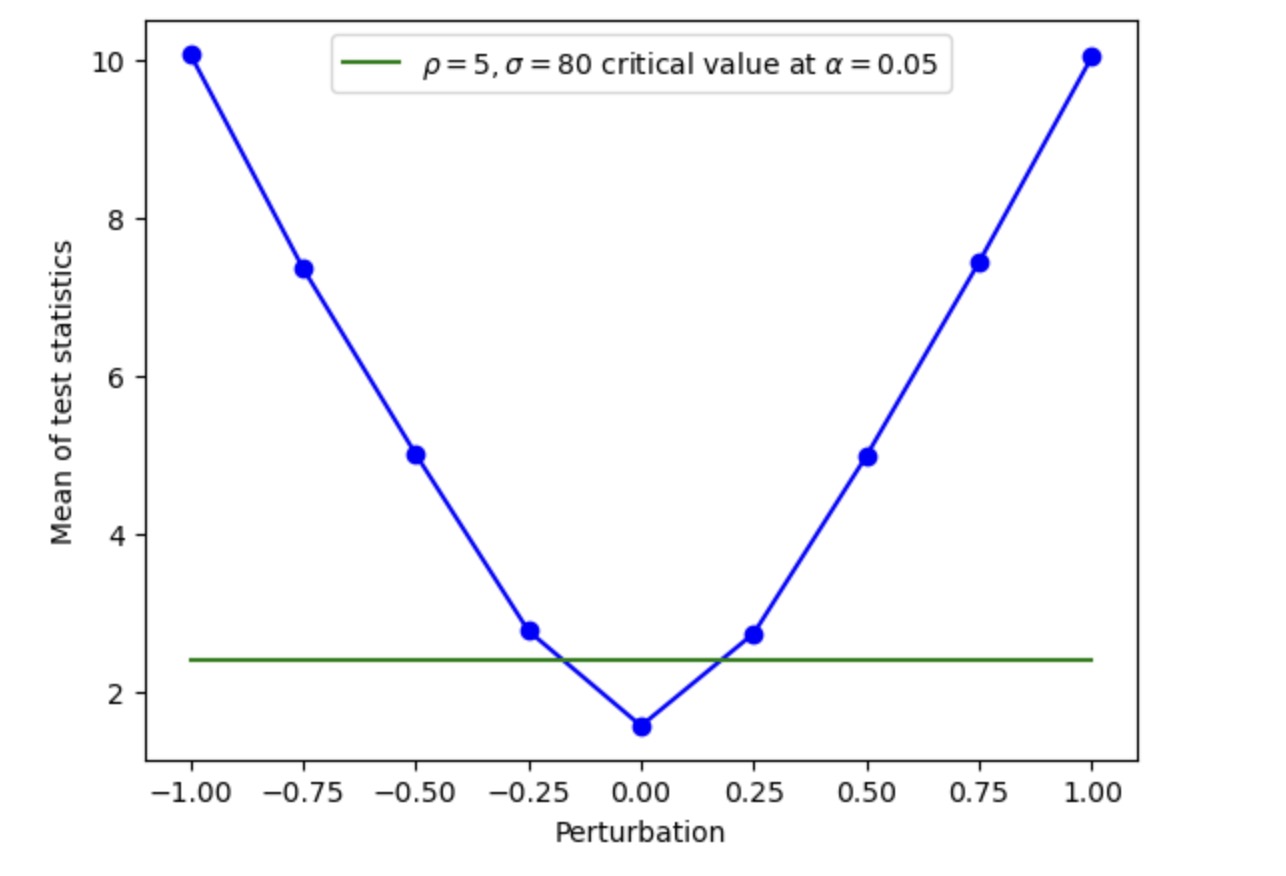
Refer to caption
(a) Rejection rate vs perturbation
Refer to caption
(b) Mean test statistics vs perturbation
Figure 6: Model 1
Refer to caption
(a) Rejection rate vs k𝑘k
Refer to caption
(b) Mean test statistics vs k𝑘k
Figure 7: Model 2

5.2 Applications

Our hypothesis test for martingality provides valuable information in a wide range of areas of interest. For instance, it is well-known that martingales form an important pillar in financial economics and econometrics. For example, no-arbitrage conditions are equivalent in great generality to requiring the existence of a suitable probability measure under which discounted price processes follow martingale dynamics. Our results, therefore, can be used (as we shall illustrate) to test the no-arbitrage hypothesis in generative AI models.

A classical problem in econometrics and statistics consists of testing if a real-valued data set follows a given continuous distribution. The Kolmogorov-Smirnov statistic is a non-parametric approach to testing this hypothesis. A natural generalization of this problem consists of testing if a positive recurrent and irreducible general state-space Markov chain with stationary distribution ϕitalic-ϕ\phi, {Wn:n⩾0}fragments{W𝑛:n0}\left\{W_{n}:n\geqslant 0\right\}, follows the transition kernel {K(x,⋅):x∈S}fragments{K(x,⋅):xS}\left\{K\left(x,\cdot\right):x\in S\right\}. This is true if and only if for all continuous and bounded functions u(⋅)fragmentsu(⋅)u\left(\cdot\right) we have (Xn,Yn)=(Wn,Wn+u(Wn+1)−(Ku)(Wn))fragments(X𝑛,Y𝑛)(W𝑛,W𝑛u(Wfragmentsn1)(Ku)(W𝑛))\left(X_{n},Y_{n}\right)=\left(W_{n},W_{n}+u\left(W_{n+1}\right)-\left(Ku\right)\left(W_{n}\right)\right) forms a martingale pair for almost every WnfragmentsW𝑛W_{n} with respect to ϕitalic-ϕ\phi. Therefore, this hypothesis can be tested by selecting a family of functions u1,…,udfragmentsu1,…,u𝑑u_{1},\dots,u_{d} and testing the martingale property for the pair of d𝑑d-dimensional vectors (Xn,Yn)∈ℝd×ℝdfragments(X𝑛,Y𝑛)R𝑑R𝑑\left(X_{n},Y_{n}\right)\in\mathbb{R}^{d}\times\mathbb{R}^{d}, where Xn(i)=WnfragmentsX𝑛(i)W𝑛X_{n}\left(i\right)=W_{n} and Yn(i)=Wn+ui(Wn+1)−(Kui)(Wn)fragmentsY𝑛(i)W𝑛u𝑖(Wfragmentsn1)(Ku𝑖)(W𝑛)Y_{n}\left(i\right)=W_{n}+u_{i}\left(W_{n+1}\right)-\left(Ku_{i}\right)\left(W_{n}\right).444The choice of uifragmentsu𝑖u_{i}’s may depend on K𝐾K. This is beyond the scope of our focus here.

The above two applications of our test will be respectively detailed in this section below and Appendix A. There are numerous other applications of martingale pair tests in the sphere of finance, econometrics, reinforcement learning, and non-parametric regression. We briefly discuss a few instances below.

In the context of model-based reinforcement learning, a simulation environment generated according to a suitable family of Markov kernels KθfragmentsK𝜃K_{\theta} (indexed by a parametric family of policies encoded by the parameter θ𝜃\theta) can be used to train an optimal control policy for the task at hand and an associated optimal value function v𝑣v, which solves a corresponding HJB equation. A suitable transformation of the value function v𝑣v (similar to that discussed in the previous paragraph for u𝑢u) can be obtained based on its associated HJB equation to define a pair (Xn,Yn)fragments(X𝑛,Y𝑛)(X_{n},Y_{n}) following a martingale sequence in the optimized simulation environment. If the simulated environment closely reflects the true environment, our results can be used to test if such a policy generates the desired performance (i.e. the predicted value v𝑣v) in a real environment by applying the policy and also transformation in the real environment, collecting the generated data in an experiment in the true environment, and testing the martingale hypothesis in the data collected by the use of the policy in the true environment.

Other applications include assessing the quality of a non-parametric regression function. Suppose that a non-parametric estimator of g(Z)=𝔼[Y|Z]fragmentsg(Z)E[Y|Z]g(Z)=\mathbb{E}[Y|Z] based on observations (Zi,Yi):i⩽nfragments(Z𝑖,Y𝑖):in{(Z_{i},Y_{i}):i\leqslant n} is produced. Now consider the problem of evaluating the quality of such a non-parametric estimator, say f0fragmentsf0f_{0}. We may consider defining X=f0(Z)fragmentsXf0(Z)X=f_{0}(Z) and then testing whether the corresponding empirical measure ℙnfragmentsP𝑛\mathbb{P}_{n} of pairs (Xi,Yi)=(f0(Zi),Yi)fragments(X𝑖,Y𝑖)(f0(Z𝑖),Y𝑖)(X_{i},Y_{i})=(f_{0}(Z_{i}),Y_{i}) is sufficiently close to the martingale space. Moreover, as we shall explain, the power analysis of the martingale projection test also provides insight into how the martingale property fails to be satisfied. This may suggest a way to improve regression estimation training.

5.2.1 Testing no-arbitrage in neural SDE-based European option calibration

One application of our results is a test for arbitrage opportunities in existing pricing models for financial derivatives. In the following, we first describe the set-up of the financial market considered and then outline our methodology.

The work of [gierjatowicz2020robust] develops a neural SDE-based European option calibration method. In their set-up, the true dynamics of X𝑋X under the risk-neutral measure ℚ=ℚ(θ)fragmentsQQ(θ)\mathbb{Q}=\mathbb{Q}(\theta) are given by

dXθt=b(t,Xθt,θ)dt+σ(t,Xθt,θ)dWtfragmentsdX𝜃𝑡b(t,X𝜃𝑡,θ)dtσ(t,X𝜃𝑡,θ)dW𝑡\displaystyle\mathrm{d}X^{\theta}_{t}=b(t,X^{\theta}_{t},\theta)\mathrm{d}t+\sigma(t,X^{\theta}_{t},\theta)\mathrm{d}W_{t} (59)

for functions b:ℝ+×ℝd×Θ→ℝdfragmentsb:RR𝑑Θ→R𝑑b:\mathbb{R}_{+}\times\mathbb{R}^{d}\times\Theta\rightarrow\mathbb{R}^{d} and σ:ℝ+×ℝd×Θ→ℝd×nfragmentsσ:RR𝑑Θ→Rfragmentsdn\sigma:\mathbb{R}_{+}\times\mathbb{R}^{d}\times\Theta\rightarrow\mathbb{R}^{d\times n}, where Θ⊆ℝpfragmentsΘR𝑝\Theta\subseteq\mathbb{R}^{p} for some p>0fragmentsp0p>0.

In order to calibrate asset prices consistently with the real-world measure ℙ(θ)fragmentsP(θ)\mathbb{P}(\theta), [gierjatowicz2020robust] introduces a feed-forward neural network trained on market data, given by ζ:[0,T]×ℝd×ℝp→ℝnfragmentsζ:[0,T]R𝑑R𝑝→R𝑛\zeta:[0,T]\times\mathbb{R}^{d}\times\mathbb{R}^{p}\rightarrow\mathbb{R}^{n}. Let dKfragmentsd𝐾d_{K} represent the discounted payoff of a call option with strike K𝐾K. The authors assume that the call prices at time zero

𝔭(dK):=𝔼ℚ(θ)[dK]=e−rT𝔼ℚ(θ)[(ST−K)+∣S0=1]fragmentsp(d𝐾)assignEfragmentsQ(θ)[d𝐾]efragmentsrTEfragmentsQ(θ)[(S𝑇K)∣S01]\displaystyle\mathfrak{p}(d_{K}):=\mathbb{E}^{\mathbb{Q}(\theta)}[d_{K}]=e^{-rT}\mathbb{E}^{\mathbb{Q}(\theta)}\left[\left(S_{T}-K\right)_{+}\mid S_{0}=1\right] (60)

are given, and they calibrate (59) to 𝔭(dK)fragmentsp(d𝐾)\mathfrak{p}(d_{K}) through finding θ∗fragmentsθ\theta^{*} such that

e−rT𝔼ℚ(θ∗)[(ST−K)+∣S0=1]≈𝔭(dK).fragmentsefragmentsrTEfragmentsQ(θ)[(S𝑇K)∣S01]p(d𝐾).\displaystyle e^{-rT}\mathbb{E}^{\mathbb{Q}(\theta^{*})}\left[\left(S_{T}-K\right)_{+}\mid S_{0}=1\right]\approx\mathfrak{p}(d_{K}).

Importantly, [gierjatowicz2020robust] only calibrates to call prices at time zero and does not take any other market data into account. In practice however, it is reasonable to assume that, next to the price process (St)t∈{0,…,T}fragments(S𝑡)fragmentst{0,…,T}(S_{t})_{t\in\{0,...,T\}}, one should also be able to observe the corresponding option prices

𝔭(dK,St)=e−rT𝔼ℚ(θ)[(ST−K)+∣St]fragmentsp(d𝐾,S𝑡)efragmentsrTEfragmentsQ(θ)[(S𝑇K)∣S𝑡]\displaystyle\mathfrak{p}(d_{K},S_{t})=e^{-rT}\mathbb{E}^{\mathbb{Q}(\theta)}\left[\left(S_{T}-K\right)_{+}\mid S_{t}\right] (61)

for t∈{0,…,T}fragmentst{0,…,T}t\in\{0,\dots,T\} instead. Armed with our martingale pair test, we will check if the calibration procedure of [gierjatowicz2020robust] is consistent with the additional prices given in (61). In other words, does

𝔭(dK,St)≈e−rT𝔼ℚ(θ∗)[(ST−K)+∣St]?fragmentsp(d𝐾,S𝑡)efragmentsrTEfragmentsQ(θ)[(S𝑇K)∣S𝑡]?\mathfrak{p}(d_{K},S_{t})\approx e^{-rT}\mathbb{E}^{\mathbb{Q}(\theta^{*})}\left[\left(S_{T}-K\right)_{+}\mid S_{t}\right]?

Our objective is to test if (𝔭(dK,St),e−rT(ST−K)+)fragments(p(d𝐾,S𝑡),efragmentsrT(S𝑇K))(\mathfrak{p}(d_{K},S_{t}),e^{-rT}\left(S_{T}-K\right)_{+}) is a martingale coupling under ℚ(θ∗)fragmentsQ(θ)\mathbb{Q}(\theta^{*}) (which is necessary for (61)) for vanilla options. Our task is composed of three steps:

  1. 1.

    Calibrate asset prices for each time-step following the algorithms of [gierjatowicz2020robust]. Obtain N𝑁N calibrated stock trajectories {St}t∈[0,…,T].fragments{S𝑡}fragmentst[0,…,T].\{S_{t}\}_{t\in[0,\dots,T]}.

  2. 2.

    Given a stock trajectory {St}t∈[0,…,T]fragments{S𝑡}fragmentst[0,…,T]\{S_{t}\}_{t\in[0,\dots,T]} from step one, use Monte Carlo simulation to obtain prices of vanilla options 𝔭(dK,St)fragmentsp(d𝐾,S𝑡)\mathfrak{p}(d_{K},S_{t}) at each t⩾0fragmentst0t\geqslant 0 using (61).

  3. 3.

    Apply the martingale pair test to check if (𝔭(dK,St),e−rT(ST−K)+)fragments(p(d𝐾,S𝑡),efragmentsrT(S𝑇K))(\mathfrak{p}(d_{K},S_{t}),e^{-rT}\left(S_{T}-K\right)_{+}) is a martingale coupling under ℚ(θ∗).fragmentsQ(θ).\mathbb{Q}(\theta^{*}).

The work of [gierjatowicz2020robust] used two market models for calibration: the local stochastic volatility model (LSV) and the local volatility model (LV). For step one, we alter the training algorithm of [gierjatowicz2020robust] for both LSV and LV models to return N=4000fragmentsN4000N=4000 calibrated stock trajectories {(St)t∈[0,…,T]i}i=1Nfragments{(S𝑡)fragmentst[0,…,T]𝑖}fragmentsi1𝑁\{(S_{t})_{t\in[0,\dots,T]}^{i}\}_{i=1}^{N} directly. The altered codes, along with the implementation codes can be found on GitHub. For step two, for each stock trajectory {St}t∈{0,…,T}fragments{S𝑡}fragmentst{0,…,T}\{S_{t}\}_{t\in\{0,...,T\}}, we use Monte Carlo simulation to generate n=1000fragmentsn1000n=1000 asset price paths using the true Heston model approximated via a tamed Euler scheme at each time point t∈{0,…,T}fragmentst{0,…,T}t\in\{0,...,T\}:

dStfragmentsdS𝑡\displaystyle\mathrm{d}S_{t} =rStdt+StVtdWt,X0=x0fragmentsrS𝑡dtS𝑡fragmentsV𝑡dW𝑡,X0x0\displaystyle=rS_{t}\mathrm{d}t+S_{t}\sqrt{V_{t}}\mathrm{d}W_{t},\ \ X_{0}=x_{0}
dVtfragmentsdV𝑡\displaystyle\mathrm{d}V_{t} =κ(μ−Vt)dt+ηVtdBt,V0=v0fragmentsκ(μV𝑡)dtηfragmentsV𝑡dB𝑡,V0v0\displaystyle=\kappa(\mu-V_{t})\mathrm{d}t+\eta\sqrt{V_{t}}\mathrm{d}B_{t},\ \ V_{0}=v_{0}
d⟨B,W⟩tfragmentsd⟨B,W⟩𝑡\displaystyle\mathrm{d}\langle B,W\rangle_{t} =ρdt.fragmentsρdt.\displaystyle=\rho\mathrm{d}t.

We use the same set of parameters as [gierjatowicz2020robust]: θ={x0=1,r=0.025,V0=0.04,κ=0.78,μ=0.11,η=0.68,ρ=0.044}fragmentsθ{x01,r0.025,V00.04,κ0.78,μ0.11,η0.68,ρ0.044}\theta=\{x_{0}=1,r=0.025,V_{0}=0.04,\kappa=0.78,\mu=0.11,\eta=0.68,\rho=0.044\}. We then calculate the associated discounted European option prices with each maturity T𝑇T and strike K𝐾K by

𝔭(dK,St):=e−rT𝔼ℚ(θ)[(ST−K)+|St]fragmentsp(d𝐾,S𝑡)assignefragmentsrTEfragmentsQ(θ)[(S𝑇K)|S𝑡]\displaystyle\mathfrak{p}(d_{K},S_{t}):=e^{-rT}\mathbb{E}^{\mathbb{Q}(\theta)}[(S_{T}-K)^{+}|S_{t}]

In addition, we also calculate the calibrated payoff using [gierjatowicz2020robust]’s formula in (60). The algorithm is in Appendix B.

For the final step, we conduct a martingale pair test of the coupling (𝔭(dK,St),e−rT(ST−K)+)fragments(p(d𝐾,S𝑡),efragmentsrT(S𝑇K))(\mathfrak{p}(d_{K},S_{t}),e^{-rT}\left(S_{T}-K\right)_{+}) fixing σ=1,ρ=5fragmentsσ1,ρ5\sigma=1,\rho=5 and a significance level of α=0.05fragmentsα0.05\alpha=0.05. We adapt the testing procedures outlined in Algorithm LABEL:algo:mtgl_pair_test. Codes for the martingale pair test can be found on our GitHub.

We find that, both for LV-model-based calibration and LSV-model-based calibration, (𝔭(dK,St),e−rT(ST−K)+)fragments(p(d𝐾,S𝑡),efragmentsrT(S𝑇K))(\mathfrak{p}(d_{K},S_{t}),e^{-rT}\left(S_{T}-K\right)_{+}) do not form martingales. For the LV model and the LSV model, the test statistics are 17.242 and 11.714 respectively, against an α=0.05fragmentsα0.05\alpha=0.05 critical value cα=fragmentsc𝛼c_{\alpha}= 4.705. In conclusion, [gierjatowicz2020robust]’s calibration method is shown to be inconsistent with the market data available.

We also observe that one of the [gierjatowicz2020robust]’s key contributions using hedging strategy as a control variate for the calibration model fails to work when we examine option prices as a function of the stock price observed at each time point. Instead, to avoid creating arbitrage opportunities in option prices (61), we propose the following neural SDE-based option calibration method: as before, the market data (input data) is represented by (discounted) payoffs {dKi}i=1Mfragments{dfragmentsK𝑖}fragmentsi1𝑀\{d_{K_{i}}\}_{i=1}^{M} of liquid derivatives and their corresponding market prices {𝔭(dKi)}i=1Mfragments{p(dfragmentsK𝑖)}fragmentsi1𝑀\{\mathfrak{p}(d_{K_{i}})\}_{i=1}^{M}. We then replace the loss function [gierjatowicz2020robust, equation (2.5)] by a martingale projection loss criterion:

θ∗∈arg minθ∈Θ∑j=1M∑i=1N∫((𝔭(dKj,Sθti)−dKj(Sti+τθ))fξ(x−dKj(Sti+τθ)))2dx.fragmentsθarg minfragmentsθΘfragmentsj1𝑀fragmentsi1𝑁((p(d𝐾𝑗,S𝜃fragmentst𝑖)d𝐾𝑗(Sfragmentst𝑖τ𝜃))f𝜉(xd𝐾𝑗(Sfragmentst𝑖τ𝜃)))2dx.\displaystyle\theta^{*}\in\text{arg min}_{\theta\in\Theta}\sum_{j=1}^{M}\sum_{i=1}^{N}\int\Big{(}(\mathfrak{p}({d_{K}}_{j},S^{\theta}_{t_{i}})-{d_{K}}_{j}(S_{t_{i}+\tau}^{\theta}))f_{\xi}(x-{d_{K}}_{j}(S_{t_{i}+\tau}^{\theta}))\Big{)}^{2}\,\mathrm{d}x.

The tentative new algorithm described by the pseudo-code can be found in Appendix B.

Appendix A Testing concurrence of a Markov chain with given transition kernel

We consider the problem of testing if an ergodic sequence follows a particular Markov chain dynamics. This problem is the analogue to the problem of testing if an i.i.d. sequence follows a particular distribution. In the one-dimensional i.i.d. setting, the Kolmogorov-Smirnov test provides a well-known approach.

Precisely, we are interested in testing if a ϕitalic-ϕ\phi-irreducible and positive recurrent Markov chain sequence {Wn:n⩾0}fragments{W𝑛:n0}\left\{W_{n}:n\geqslant 0\right\} taking values on a state-space S𝑆S (e.g. the support of ϕitalic-ϕ\phi, which may be assumed to be a maximal irreducible measure) follows a particular transition kernel, {K(x,⋅):x∈S}fragments{K(x,⋅):xS}\left\{K\left(x,\cdot\right):x\in S\right\}. This is true if and only if for all continuous and bounded functions u(⋅)fragmentsu(⋅)u\left(\cdot\right) we have that

(Xn,Yn)=(Wn,Wn+u(Wn+1)−(Ku)(Wn))fragments(X𝑛,Y𝑛)(W𝑛,W𝑛u(Wfragmentsn1)(Ku)(W𝑛))\left(X_{n},Y_{n}\right)=\left(W_{n},W_{n}+u\left(W_{n+1}\right)-\left(Ku\right)\left(W_{n}\right)\right)

forms a martingale pair for almost every WnfragmentsW𝑛W_{n} with respect to ϕitalic-ϕ\phi. Indeed, if the ergodic chain satisfies this condition we have that for all continuous and bounded functions u(⋅)fragmentsu(⋅)u\left(\cdot\right)

(Ku)(Wn)=E[u(Wn+1)|Wn]fragments(Ku)(W𝑛)E[u(Wfragmentsn1)|W𝑛]\left(Ku\right)\left(W_{n}\right)=E\left[u\left(W_{n+1}\right)|W_{n}\right]

almost everywhere with respect to the stationary measure which is a maximal irreducible measure (see Theorems 10.0.1 and 10.1.2 in [meyn2009]).

As an application of our results in this paper, we can select a family of continuous and bounded functions u1,…,udfragmentsu1,…,u𝑑u_{1},\dots,u_{d} so we can test the martingale property for the pair of d𝑑d-dimensional vectors (Xn,Yn)∈ℝd×ℝdfragments(X𝑛,Y𝑛)R𝑑R𝑑\left(X_{n},Y_{n}\right)\in\mathbb{R}^{d}\times\mathbb{R}^{d}, where

Xn(i)=Wn, Yn(i)=Wn+ui(Wn+1)−(Kui)(Wn).fragmentsX𝑛(i)W𝑛, Y𝑛(i)W𝑛u𝑖(Wfragmentsn1)(Ku𝑖)(W𝑛).X_{n}\left(i\right)=W_{n},\text{ }Y_{n}\left(i\right)=W_{n}+u_{i}\left(W_{n+1}\right)-\left(Ku_{i}\right)\left(W_{n}\right).

To put the discussion into context, we consider a simple Gaussian Markov process and an example inspired by the present value process of perpetual cash flow as described in Example 2.2 of [gjessing1997present].

Example 8 (Gaussian Markov Process).

Consider the simple case of an infinite state space Gaussian Markov Process as the following:

Xn+1=κXn+ξn+1,fragmentsXfragmentsn1κX𝑛ξfragmentsn1,X_{n+1}=\kappa X_{n}+\xi_{n+1},

where κ∈[0,1]fragmentsκ[0,1]\kappa\in[0,1], ξn+1∼𝒩(0,1)fragmentsξfragmentsn1similar-toN(0,1)\xi_{n+1}\sim\mathcal{N}(0,1) for each n∈ℕfragmentsnNn\in\mathbb{N}.

Choosing u1(x)=xfragmentsu1(x)xu_{1}(x)=x and u2(x)=x𝟙{x>0}fragmentsu2(x)x1fragments{x0}u_{2}(x)=x\mathds{1}_{\{x>0\}}, we generate {(Xn,Xn+1)}n=11000fragments{(X𝑛,Xfragmentsn1)}fragmentsn11000\{(X_{n},X_{n+1})\}_{n=1}^{1000} with κ=0.5fragmentsκ0.5\kappa=0.5. For a martingale pair test with parameters {ρ=5,σ=1,α=0.05}fragments{ρ5,σ1,α0.05}\{\rho=5,\sigma=1,\alpha=0.05\}, the loss of the series of couplings is 3.091e-23 against an asymptotic cutoff value of 4.840. Hence, the test correctly accepts the series {(Xn,Xn+1)}n=11000fragments{(X𝑛,Xfragmentsn1)}fragmentsn11000\{(X_{n},X_{n+1})\}_{n=1}^{1000} as a martingale with 95% confidence.

Example 9 (Adapted present value process of perpetual cash flow).

Consider the stochastic process

Zt=e−rt(Z0+∫s=0tersdPs)fragmentsZ𝑡efragmentsrt(Z0fragmentss0𝑡efragmentsrsdP𝑠)\displaystyle{Z}_{t}\ =e^{-rt}\Big{(}Z_{0}+\int_{s=0}^{t}e^{rs}\mathrm{d}{P_{s}}\Big{)} (62)

where t⩾0fragmentst0t\geqslant 0, r>0fragmentsr0r>0, Z0=0fragmentsZ00Z_{0}=0, and Pt=∑i=1NP,tSP,ifragmentsP𝑡fragmentsi1fragmentsNfragmentsP,tSfragmentsP,i{P}_{t}=\sum_{i=1}^{N_{P,t}}S_{P,i} is a non-negative compound Poisson process with NP,t∼Pois(λP)fragmentsNfragmentsP,tsimilar-toPois(λ𝑃)N_{P,t}\sim\text{Pois}(\lambda_{P}) and SP,i∼Γ(α,β)fragmentsSfragmentsP,isimilar-toΓ(α,β)S_{P,i}\sim\Gamma(\alpha,\beta). Choose r=1fragmentsr1r=1, λP=2fragmentsλ𝑃2\lambda_{P}=2 and (α,β)=(2,3)fragments(α,β)(2,3)(\alpha,\beta)=(2,3), where α𝛼\alpha denotes the location parameter and β𝛽\beta denotes the scale parameter.

To generate the Markov chain, we use the observation that

Zt+1=Zt+∫s=01er(s−t)dPt+s.fragmentsZfragmentst1Z𝑡fragmentss01efragmentsr(st)dPfragmentsts.\displaystyle Z_{t+1}=Z_{t}+\int_{s=0}^{1}e^{r(s-t)}\mathrm{d}P_{t+s}.

Choosing u1(x)=xfragmentsu1(x)xu_{1}(x)=x and u2(x)=x𝟙{x>0}fragmentsu2(x)x1fragments{x0}u_{2}(x)=x\mathds{1}_{\{x>0\}}, we generate {(Zt,Zt+1)}t=11000fragments{(Z𝑡,Zfragmentst1)}fragmentst11000\{(Z_{t},Z_{t+1})\}_{t=1}^{1000}. For a martingale pair test with parameters {ρ=5,σ=1,α=0.05}fragments{ρ5,σ1,α0.05}\{\rho=5,\sigma=1,\alpha=0.05\}, the loss of the series of couplings is 1.036 against an asymptotic cutoff value of 4.840. Hence, the test correctly accepts the series {(Zt,Zt+1)}t=11000fragments{(Z𝑡,Zfragmentst1)}fragmentst11000\{(Z_{t},Z_{t+1})\}_{t=1}^{1000} as a martingale with 95% confidence.

It is interesting to note that the modified version of stochastic process (62)

Zt=∫0te−rsdPsfragmentsZ𝑡0𝑡efragmentsrsdP𝑠\displaystyle Z_{t}=\int_{0}^{t}e^{-rs}\mathrm{d}P_{s}

has financial implications. In this case, Z∞fragmentsZ{Z}_{\infty} has the following density (see [gjessing1997present]):

fZ∞=α12(1+γ)γ12(1−γ)e−γz12(γ−1)Iγ−1(2αγz)eαz,fragmentsffragmentsZαfragments12(1γ)γfragments12(1γ)efragmentsγzfragments12(γ1)Ifragmentsγ1(2fragmentsαγz)efragmentsαz,\displaystyle f_{{Z}_{\infty}}=\alpha^{\frac{1}{2}(1+\gamma)}\gamma^{\frac{1}{2}(1-\gamma)}e^{-\gamma}z^{\frac{1}{2}(\gamma-1)}I_{\gamma-1}(2\sqrt{\alpha\gamma z})e^{\alpha z},

where γ=λP/rfragmentsγλ𝑃r\gamma={\lambda_{P}}/{r} and λPfragmentsλ𝑃\lambda_{P} denotes the intensity of NP,tfragmentsNfragmentsP,tN_{P,t}, and I𝐼I is the modified Bessel function of the first kind of order γ𝛾\gamma:

Iγ(x)=(x2)γ∑k=0∞1k!Γ(k+γ+1)(x2)2k.fragmentsI𝛾(x)(𝑥2)𝛾fragmentsk01fragmentskΓ(kγ1)(𝑥2)fragments2k.\displaystyle I_{\gamma}(x)=(\frac{x}{2})^{\gamma}\sum_{k=0}^{\infty}\frac{1}{k!\Gamma(k+\gamma+1)}(\frac{x}{2})^{2k}.

In an actuarial context, PtfragmentsP𝑡{P}_{t} is interpreted as the surplus generating process and Z∞fragmentsZ{Z}_{\infty} represents the present value of perpetual cash flow with respect to PtfragmentsP𝑡{P}_{t}.

Appendix B Deferred algorithms

Algorithm 1 Simulate Asymptotic Distribution given {ρ,σ}fragments{ρ,σ}\{\rho,\sigma\}

Input: total number of grid points n𝑛n per dimension d𝑑d, total number of simulations N𝑁N, domain of integration [xmin,xmax]dfragments[x,x]𝑑[x_{\min},x_{\max}]^{d}, samples of martingale couplings (X,Y)fragments(X,Y)(X,Y), martingale projection parameters {ρ,σ}fragments{ρ,σ}\{\rho,\sigma\}.
Initialization: initialize grid g={g1,…,gnd}fragmentsg{g1,…,gfragmentsn𝑑}g=\{g_{1},\dots,g_{n^{d}}\} based on domain of integration [xmin,xmax]dfragments[x,x]𝑑[x_{\min},x_{\max}]^{d} and number of grid points n𝑛n, smoothing kernel fσ,ξ,ρfragmentsffragmentsσ,ξ,ρf_{\sigma,\xi,\rho} as defined in (4).

Given samples (X,Y)fragments(X,Y)(X,Y), grid g𝑔g, and fσ,ξ,ρfragmentsffragmentsσ,ξ,ρf_{\sigma,\xi,\rho}:
for index i𝑖i 1:ndfragments1:n𝑑1:n^{d} do
     for index j𝑗j 1:ndfragments1:n𝑑1:n^{d} do
         Generate each entry (i,j)fragments(i,j)(i,j) of the covariance matrix Mn×nfragmentsMfragmentsnnM_{n\times n} of Gaussian random field {Gx}fragments{G𝑥}\{G_{x}\}:
𝔼[GgiGTgj]=𝔼[(Y−X)fσ,ξ,ρ(gi−X)fσ,ξ,ρ(gj−X)(Y−X)T].fragmentsE[Gfragmentsg𝑖G𝑇fragmentsg𝑗]E[(YX)ffragmentsσ,ξ,ρ(g𝑖X)ffragmentsσ,ξ,ρ(g𝑗X)(YX)𝑇].\mathbb{E}[G_{g_{i}}G^{T}_{g_{j}}]=\mathbb{E}[(Y-X)f_{\sigma,\xi,\rho}(g_{i}-X)f_{\sigma,\xi,\rho}(g_{j}-X)(Y-X)^{T}].
     end for
end for
for index i𝑖i 1:Nfragments1:N1:N do
     Compute a sample
Si=∫x∈g∥Gx∥2dx.fragmentsS𝑖fragmentsxg∥G𝑥∥2dx.S_{i}=\int_{x\in g}\|G_{x}\|_{2}\mathrm{d}x.
end for
return {Si}i=1Nfragments{S𝑖}fragmentsi1𝑁\{S_{i}\}_{i=1}^{N}.
Conversion to HTML had a Fatal error and exited abruptly. This document may be truncated or damaged.