supple
Learn What You Need
in Personalized Federated Learning
Abstract
Personalized federated learning aims to address data heterogeneity across local clients in federated learning. However, current methods blindly incorporate either full model parameters or predefined partial parameters in personalized federated learning. They fail to customize the collaboration manner according to each local client’s data characteristics, causing unpleasant aggregation results. To address this essential issue, we propose Learn2pFed, a novel algorithm-unrolling-based personalized federated learning framework, enabling each client to adaptively select which part of its local model parameters should participate in collaborative training. The key novelty of the proposed Learn2pFed is to optimize each local model parameter’s degree of participant in collaboration as learnable parameters via algorithm unrolling methods. This approach brings two benefits: 1) mathmatically determining the participation degree of local model parameters in the federated collaboration, and 2) obtaining more stable and improved solutions. Extensive experiments on various tasks, including regression, forecasting, and image classification, demonstrate that Learn2pFed significantly outperforms previous personalized federated learning methods.
Index Terms:
Personalized federated learning, algorithm unrolling, data heterogeneity.I Introduction
Federated learning (FL) is an emerging collaboration paradigm that was first introduced in [1]. In the classical FL framework, local clients receive an identical global model from the server and conduct independent local model training on their respective datasets. Subsequently, they send their individual models back to the server for further model aggregation, which is performed there. This iterative process between the server and local clients, as shown in Fig. 1(a), persists until achieving a satisfying global model. Since only an update to the current global model is uploaded in FL, instead of raw datasets, it can protect data privacy in some degree. Due to this characteristic, it is widely used in finance [2], healthcare [3], smart cities [4], video surveillance [5] and other fields. However, data heterogeneity [6, 7, 8] across local clients creates deviations between local models and the global model so that they cannot reach the consensus, which is also referred to as client drift [9]. Besides, there is a lack of solution personalization for practical applications in classical FL [10]. Hence, personalized federated learning [10, 11] has been widely explored to train improved local models within the FL framework, instead of relying solely on a global model.

Previous research in personalized federated learning aims to address data heterogeneity across local clients in federated learning by mainly two approaches: 1) personalizing the global model and 2) learning the personalized model. The first approach focuses on generalizing the global model and local adaptation. It involves training a single global model that is then applied in downstream tasks, in line with established FL techniques such as FedAvg [1] and FedProx [12], using techniques like finetuning (FT) and knowledge transfer [7] across all local model parameters as shown in Fig. 1(a). While effective, this approach may not fully capture the unique characteristics of individual clients’ data. The second approach, which our method belongs to, aims to provide personalized solutions within the federated learning framework. By modifying the learning process with full model parameters in FL, these model-based personalized FL methods are presented in a variety of ways, e.g., optimization on the well-designed objective functions [13, 14, 15], meta-learning [16], clustering [17, 18], generative networks [19], etc. Among them, some works [20, 21, 22, 23, 24] realize that personalization with full parameters may be unnecessary, and manually divide them into personal parameters and shared parameters, where only the former is updated locally, as illustrated in Fig. 1(b). However, these works do not examine to what degree these chosen partial parameters should be integrated into the federated learning process. The limited variability caused by binary selection hinders the creation of personalized models that could better adapt to local data.
Motivated by this, we aim to learn to determine which part of a local model should participate in federated learning and further to what degree, as illustrated in Fig. 1(c). To achieve this, our key idea is to consider each parameter’s degree of participant in collaboration as one learnable variable, and then optimizes those parameters in algorithm unrolling. Following this spirit, we propose a novel algorithm-unrolling-based personalized federated learning framework, Learn2pFed. Specifically, it unrolls the parameters, originally in the iterative algorithm that can indicate the degree of participant in collaboration, into layers of a deep network. Supervised by the sum of training losses collected from all local clients, Learn2pFed adaptively learns the characteristics of the local data and select appropriate partial parameters.
Different from the previous works enabling clients to adaptively share partial model parameters from a whole candidate set, including methods such as parameter prunning [25, 26], and subnet training [27, 28], we adaptively learn local parameters that are fixed in other methods in FL framework, e.g., the aggregated weights, by algorithm unrolling, which makes learning personalized models more challenging. To sum up, Learn2pFed has two distinct advantages: 1) it dynamically determines which parameters of the local model need to collaborate in FL and to what degree, thus adapting to the local data better and improving the performance of personalized FL; and 2) it leverages algorithm unrolling to make hyper-parameters learnable and significantly improves the model capability.
To evaluate Learn2pFed, we consider various personalized FL tasks including regression, forecasting and image classification on different datasets: synthetic polynomial data, power consumption data, Fashion-MNIST [29] and CIFAR-10 [30]. Learn2pFed outperforms the previous personalized FL methods in the above three tasks.
Our main contributions are three-fold:
-
1.
We introduce adaptive collaboration in personalized federated learning by enabling each client to select which part of its local model parameters should participate in personalized federated learning, addressing data heterogeneity and improving aggregation results.
-
2.
We propose a novel algorithm-unrolling-based framework Learn2pFed for personalized federated learning to optimize the degree of participant for each model parameter in collaboration, which turns the fixed hyper-parameters in the optimization into learnable parameters in our framework.
-
3.
We conduct extensive experiments in various tasks, and show that the performance is competitive with state-of-the-art methods.
This article is organized as the following. Section II reviews the related works. Section III presents several preliminaries about personalized FL. Section IV introduces our proposed Learn2pFed method, including algorithm design, federated implementation, theoretical analysis and extensive discussion. Section V shows the experimental results in three different tasks. And the conclusion goes to Section VI.
II Related Works
Personalized Federated Learning: Personalized federated learning [10] aims to deal with the data heterogeneity and provide personalized solutions. One popular strategy is performing model personalization from the globally shared FL model by finetuning [7], meta-learning (e.g., Per-FedAvg [16], pFedMe [13]), model interpolation (e.g., FedProx [12], SCAFFOLD [9]), transfer learning (e.g., FedMD [31], Co-MDA [32]), etc. Another strategy aims to learn personalized models that involves parameter pruning, sub-network selection and so on. Among them, FedPer [20] and FedRep [21] artificially determine the local model as base layers and personalized layers, and keep the latter private in local training to learn personalized representation. For different computation and communication capabilities, HeteroFL [27] adaptively allocating local models of different complexity levels based on the global model, and FedPM [28] learns a binary mask to find the optimal sparse random network within the original one. FedMP [25] performs model pruning, where the server adaptively determines the specific pruning ratio according to the capabilities of local clients. And PartialFed-Adaptive [26] learns the personalized loading strategy by reparameterization for each client so that the local model is a subset of the global model’s parameters. In contrast to these works, the proposed Learn2pFed is a novel framework closed to meta-learning and aims to better adapt to local data in personalized FL via learning the degree of participant in federated collaboration with algorithm unrolling.
Algorithm Unrolling: Algorithm unrolling [33] is a technique that unrolls one specific iterative optimization algorithm, e.g., the iterative shrinkage and thresholding algorithm (ISTA [34]), the alternating direction method of multipliers (ADMM [35]), into stacked layers of a deep network. Then, each forward propagation of the network is equivalent to performing several iterations of the iterative algorithm with fixed parameters. And the backward propagation of the deep model makes the fixed parameters learnable. In this way, unrolling enhances both the representation ability of the iterative algorithm and the generalization ability of the generic neural networks, thus reaching an attractive balance. For these advantages, it has been widely applied in various domains, including the context of sparse coding [36], compress sensing [37], image fusion [38] and signal denoising [39, 40, 41]. In our work, we leverage deep unrolling to determine the personal parameters in personalized federated learning, bridging the gap between iterative algorithms and the federated learning framework.
III Preliminary
The personalized FL framework consists of one parameter server and local clients, where the -th client holds the local data with generated from one of the unknown models. denotes the number of samples in the -th client and denotes the feature dimension. Let be the global model parameters, and be the -th local model parameters for , where we denote the set for any integer as .
Generally, the objective of personalized FL is formed as the local objectives given the optimized global model , composed of local empirical loss on the local training data in the -th client and the regularized term indicating the distance between the global model and local model. Mathematically, the optimization of personalized FL is typically formed as below.
| (1) | ||||
where and are two kinds of positive hyper-parameters in personalized FL, and denotes the abbreviation of . Specifically, regularizes the similarity between the global model and local models, with larger values of indicating stronger similarity. When , personalized FL degrades to the general FL; when , personalized FL degrades to the local independent learning.
While (1) provides the mathematical form commonly used in personalized federated learning methods, it has a limitation arisen from treating the entire local parameter model as a single entity, thus overlooking the unique characteristics of local data. This limitation may hamper the ability to adapt the model to individual data distributions and can result in worse performance in personalized federated learning. Therefore, it becomes crucial to address this limitation and develop a solution by learning the specific parameters of local models in collaboration.
In this regard, we propose Learn2pFed, a novel framework that entails redesigning the formulation of (1). We will delve into the details of the Learn2pFed framework in the next section.
IV Learn2pFed: Unrolling-based Personalized FL Framework
To determine which specific parameters of the local models should participate in the federated learning, this section introduces Learn2pFed, a novel deep unrolling framework for personalized federated learning from both aspects of mathematical optimization and federated implementation. We further provide its convergence analysis, and discuss its characteristics including privacy, computation burden, and communication cost.
IV-A Overall Optimization
Based on the original optimization problem (1), we introduce another crucial component, , alongside the aggregation weight variable . This addition allows us to achieve personalized regularization for each model parameter, further enhancing the adaptive federated aggregation.
Regularized variable : Instead of using a scalar in (1) to regularize all model parameters, we introduce a personalized diagonal matrix for the -th client for element-wise regularization. Each element is a positive value, indicating the degree of each model parameter that participates in the federated collaboration. This matrix enables customized regularization for different parameters within each client’s local model. Such fine-grained personalized regularization allows for adaptive control of the degree of participant in collaboration, improving model performance by tailoring the regularization to the specific characteristics of each client’s data.
Subsequently, the overall optimization of Learn2pFed is formulated as a bi-level optimization problem, which involves the learning objective and the constraint problem :
| (2) | ||||
where is the output of and denotes the local training loss in the -th client based on the specific tasks, such as Mean-Squared-Error (MSE) loss for regression or Cross-Entropy (CE) loss for classification. Intuitively, (2) aims to output the learned local model for personalized FL, while learning the adaptive collaboration pattern via learnable parameters with the supervised information in the form of the sum of local training losses. Unlike (1), (2) also includes the learning of , thus it can adaptively determine the specific part of local model parameters involved in the collaboration, allowing for a more flexible and effective personalized federated learning process.
To address the optimization problem presented in (2), we leverage algorithm unrolling. Specifically, our approach involves solving the objective of (2) using a single optimization algorithm, as discussed in Section IV-B. Subsequently, we unroll this algorithm into layers and train a deep network, as explained in Section IV-C.
IV-B Optimization Algorithm
This sub-section aims to solve the learning objective of (2) with fixed parameters . Since the global model and local models are coupled in in (2), the alternating direction method of multipliers (ADMM [35]) is a way to split the variables into local sides and the global side. Specifically, we introduce the auxiliary variable indicating the consensus constraint in the local. It brings two benefits: 1) it decouples the global and local model so that solving the local variables can be carried out in parallel in each client; 2) it allows for a more flexible expression of constraints making the problem easier to solve. Then, in (2) is reformulated as below.
| (3) | ||||
For faster convergence, we also provide its augmented Lagrangian as
| (4) | ||||
where are Lagrangian multipliers in the local and are positive hyper-parameters. That is, taking the regression problem as example where , the ADMM alternatively optimizes by solving the following sub-problems in the -th iteration.
| (6) | |||
| (8) | |||
| (10) | |||
| (12) |
Since it follows the standard ADMM, its convergence is guaranteed by [42, 43]. After performing multiple iterations, e.g., iterations, till convergence as described above, we obtain the local model .
However, determining plays a critical role in (6)-(12) since each has a distinct impact on the performance and convergence behavior. For example, the elements of control the similarity between local and global models for specific features. Tuning these elements influences the models’ behavior in capturing global patterns. Similarly, affects the convexity and underfitting of local models. Balancing is crucial to avoid overfitting or excessive similarity. But selecting suitable is challenging due to their interplay and sensitivity. Manual tuning is time-consuming and prone to biases. Moreover, directly optimizing them in the original problem is not feasible for the trivial solution. Therefore, how to determine is a big challenge, and we provide our method making them learnable in the next section.
IV-C Algorithm Unrolling
We introduce the proposed personalized FL framework Learn2pFed based on algorithm unrolling to adaptively determine the learnable parameters in the above section. The key idea is to view the parameters in (6)-(12) as trainable parameters in a deep network with the input and parameters as , where local data are privately stored in local clients. Specifically, we solve the optimization in (6)-(12) iteratively, and model one of iterations as a four-layer cell in , as illustrated in Fig. 2.

Mathematically, we provide the formulations of the intermediate outputs in the -th cell as follows.
| (13) | ||||
| (14) | ||||
| (15) | ||||
| (16) |
where means the identity matrix with the dimension , and the parameters are learnable. This is the main difference from the iterative algorithm in (6)-(12). In addition, we build up the ReLU [44] module to guarantee the diagonal element of is positive, which is given manually in the previous. In this way, the proposed Learn2pFed concatenates multiple four-layer modules as described above into the deep network. It is worth noting that the update sequence of the ADMM has little impact on its convergence, hence the decision to design the layers is for easier federated implementation.
In the training stage of Learn2pFed, we consider the following optimization problem:
| (17) |
where is the local training loss based on the output of the final layer. In contrast to in (2), introduced by the ADMM is also treated as the target variable in (17). Then, the parameters are updated iteratively through the standard gradient descent.
In conclusion, the proposed Learn2pFed framework performs the iterative algorithm in forward propagation, and trains the learnable parameters in the deep network supervised by the sum of local training losses, which carries high-level information from other clients. Learn2pFed enjoys the following benefits: 1) it adaptively learns during the training process which could not be learned from optimization aspect otherwise, enabling it to determine the degree of participation of each local model’s parameters in the collaboration. This adaptive learning capability allows the framework to dynamically adjust the collaboration strategy based on the specific characteristics of the data and the optimization problem at hand. 2) the integration of deep neural networks in Learn2pFed provides a powerful modeling capability. By leveraging the expressive power of deep networks, the framework can capture complex patterns in each local data, leading to improved performance as demonstrated in Section V.
IV-D Federated Implementation
We provide a detailed federated implementation of Learn2pFed. We initialize local learnable parameters , the local model, and its intermediate variables on the client sides, where . Additionally, we initialize global learnable parameters and the global model , with serving as a copy of on the server side. We then introduce the implementation on both client and server sides.
1) Client-Side Computation and Communication: In the client sides, Learn2pFed updates the intermediate variables by (13), (14), (15), respectively, in the -th cell of the deep network based on the learnable parameters . Note that when updating , since can be convex or non-convex, we need to discuss the solution separately, and take the two tasks that we will face in the experiments for example. In regression tasks, we perform (14) directly. However, in classification tasks, is non-linear. Then we reformulate the update of in (14) using the gradient descent as follows.
| (18) |
where we denote
based on (6). We find that the approximation accuracy of the solution in this layer does not affect the convergence of the network much in practice, so the learning rate can be artificially set.
As for the communication, each local client sends the vector and the local training loss to the server in each cell and the final cell of the network, respectively. Additionally, each client receives the global model and the sum of local training losses across clients broadcasted by the server in each cell and the final cell of the network, respectively. Finally, each client leverages the sum of losses to independently update their learnable parameters using the gradient descent method in the final cell of the network in the client sides.
2) Server-Side Computation and Communication: In the server side, Learn2pFed updates the intermediate variable by (12) in the -th cell of the deep network based on the learnable parameters . Since appears in both sides, we copy it as and update the only in the server side. In terms of communication, the server broadcasts the updated global model and the sum of local training losses back to all the clients in each cell ann the final cell of the network. At the same time, the learnable parameters are updated based on the sum of local training losses in the server side using the gradient descent method in the final cell of the network.
Then, the above computations and communications are repeated untill Learn2pFed converges. To sum up, we summarize the overall algorithm as below.
IV-E Theoretical analysis
This sub-section provides theoretical convergence analysis of Learn2pFed, including the required assumptions, lemmas and the derived theorem. Existing theoretical analyses of the convergence properties of federated learning (FL) algorithms often highlight the dependency of convergence bounds on hyper-parameters. In contrast, our approach features learnable parameters, making it challenging to provide a precise bound. As a result, our convergence analysis is divided into two components: one focuses on the convergence of forward optimization under given parameters, and the other delves into the convergence of stochastic optimization based on SGD [45]. Our basic idea is that the forward propagation of Learn2pFed converges to a stationary point given the learnable parameters, and simultaneously, the backward propagation of Learn2pFed probabilistically converges to a local minimum. Consequently, the entire network exhibits convergence.
First, we present the relationship between the primal variable and the dual variable in the forward propagation of Learn2pFed in the following lemma, and its detailed proof goes to the supplemental materials.
Lemma 1.
There exists the positive constant for , such that
Then, we present the following assumptions, which serve as the foundation for our main theorems to follow.
Assumption 1.
Suppose the hyper-parameters in the forward propagation satisfy the following conditions:
-
1.
The hyper-parameters for are large enough so that the -subproblem is strongly convex with modulus , which is a monotonic increasing function of .
-
2.
For any , the positive constant satisfies , where is the maximum value of the finite series for , so that by setting as the linear function.
Under Assumption 1, we can obtain the local convergence of the backward propagation of , which is fulfilled by SGD, with high probability to a minima of the objective function (cf. Theorem 3 and 5 in [46]). Then, we focus on the convergence of the forward propagation of under the fixed (simplified as ) in the following.
Theorem 1.
(Convergence of forward propagation.) Suppose Assumption 1 is satisfied, , }, and are denoted as the updates obtained at the -th forward iteration of Learn2pFed. We have the following:
Since the Lagrangian function value is decreasing and lower-bounded, Learn2pFed converges as .
The detailed proof goes to the supplemental materials. And the theorem indicates that the forward propagation of Learn2pFed follows the standard ADMM iterates and has a convergent subsequence. Besides, every limit point is a stationary point for the non-convex problem according to [42], which does not impose any assumptions on the iterates. To this end, we provide the convergence of the proposed algorithm.
IV-F Further Discussions
1) Privacy: Though FL framework avoids local data being exposed, the full model parameters may still leak the data privacy by various attack methods [47, 48]. However, these attacks primarily rely on the feature reconstruction of individual samples. In Learn2pFed, we adhere to the standard vertical Federated Learning (FL) framework, where the gradient is typically computed as the average over a subset of the training data. Moreover, we enhance security by transmitting the estimation of model parameters through a mixed combination of multiple local variables, thereby increasing the difficulty of these attacks.
2) Computation and Storage Burden: Our approach introduces auxiliary variables and dual variables in the forward propagation, thereby increasing computational and storage costs. While in However, when replacing only the linear layers of large networks, the model parameters count is significantly reduced, as demonstrated in our experimental results in Section V-D.
3) Communication Cost: The communication of Learn2pFed includes two streams: a) the linear combination of model parameters, whose cost is same as that of most FL methods, and b) the loss value of each client, which can be neglected since it only costs 1 unit. Besides, the proposed method is scalable because both the communication cost and computational load increases linearly with the number of clients.
V Experiments
In this section, we first conduct algorithm comparisons in a three-order polynomial regression task, and investigate the characteristics of Learn2pFed through ablation studies. Further, we apply it in both power consumption forecasting and image classification with the real-world data in various personalized FL settings and extend it to hundreds of clients, demonstrating superior performance compared to other baseline methods. All the experiments are implemented in PyTorch and simulated in NVIDIA GeForce RTX 3090 GPUs. Core codes are available in this link111https://github.com/kelenlv/Learn2pFed.
V-A Experimental Setup
Baselines. We compare our proposed Learn2pFed with representative baselines under multiple experimental settings. Local-Only indicates that each client trains an independent model using its local data without federated collaboration. FedAvg [1] and FedProx [12] are two general FL baselines, while FedAvg+FT and FedProx+FT are their fine-tuning versions. Other personalized FL baselines include FedPer [20], FedRep [21], Ditto [14], pFedMe [13], lp_proj [15], CFL [17], and KNN-per [18]. Note that cluster-based personalized FL methods like CFL and KNN-per are only used in our classification tasks.
Training Details. We consider communication rounds of FL and epochs for each round with the batch size of . We use Adam as the optimizer with a learning rate of . For regression and forecasting tasks, we build up Learn2pFed following Alg. 1 with , while using MLP and LSTM [49] as baseline models, respectively, for comparison. For image classification tasks, we use Learn2pFed as a plug-and-play model that replaces the last layer of the original CNN with a linear approximation; see more details in the supplemental materials.
| Methods | Type in FL | Averaged RMSE | ||
|---|---|---|---|---|
| Setting 1 | Setting 2 | Setting 3 | ||
| Local-Only | - | 0.0204 | 0.0149 | 0.0208 |
| FedAvg | Generalized | |||
| FedProx | Generalized | |||
| FedAvg + FT | Finetune | |||
| FedProx+ FT | Finetune | |||
| FedPer | Split layers | |||
| FedRep | Split layers | |||
| pFedMe | Optimization | |||
| Ditto | Optimization | |||
| lp_proj | Optimization | |||
| Learn2pFed | Optimization | 0.0002 0.0002 | 0.0003 0.0002 | 0.0003 0.0002 |
V-B Polynomial Regression Task
Dataset and Federated Settings. In this experiment, each client has a distinct ground-truth (gt) objective function , where is the polynomial coefficient vector. Different clients have different coefficient vectors, while they may share some coefficients. Here, we consider three different settings:
-
•
Setting 1: all clients share three coefficients, i.e., .
-
•
Setting 2: all clients share two coefficients, i.e., .
-
•
Setting 3: all clients share one coefficient, i.e., .
The remaining coefficients are set distinctly across clients. Note that since high-order coefficients can have a greater impact on the disturbance of the function, we prefer to keep the lower-order coefficients the same across clients to increase the task’s difficulty. Finally, we generate local data by adding Gaussian noise to the local gt function with a mean of 0 and a standard deviation of 0.1.
Results and Analysis. We perform the experiments for five independent trials with full 10-client participation, and report the averaged Root-Mean-Squared-Error (RMSE) results in Table I. We see that 1) the optimization-based methods, including Ditto [14] and lp_proj [15], perform better in terms of both accuracy and stability, as they exhibit smaller RMSEs and variances compared to other approaches. However, the performance of the methods varies depending on the complexity of the dataset. For example, in simpler Setting 1, Ditto and FedPer show better performance than other methods, while in the more complex Setting 3, only Ditto outperforms other methods. This suggests that the choice of the method depends on the characteristics of the dataset. 2) Notably, Learn2pFed consistently outperforms other methods in fitting the polynomial model across all experimental settings, indicating that Learn2pFed is effective in capturing the underlying patterns in the personalized data and is robust to variations in the input. More visualization results are shown in the supplemental materials.
Impact of Learnable Parameters. We aim to investigate which specific learnable parameters play a more important role in the proposed Learn2pFed by repeating the simulations for five times and show the results in Table II. It reveals that learning more learnable parameters increases the representation power of Learn2pFed and improves the performance. Further, learning in (12), which play a role like learning rates in forward propagation (13), is shown to be not helpful enough. However, learning the parameters (especially ) plays an important role in Learn2pFed since they are more concerned with the FL process.
| Learnable parameters | Averaged RMSE of Learn2pFed | |||||||
| Setting 1 | Setting 2 | Setting 3 | ||||||
| ✓ | ||||||||
| ✓ | ||||||||
| ✓ | ✓ | |||||||
| ✓ | ✓ | ✓ | ✓ | |||||
| ✓ | ||||||||
| ✓ | ||||||||
| ✓ | ||||||||
| ✓ | ||||||||
| ✓ | ✓ | ✓ | ✓ | ✓ | ||||
| ✓ | ✓ | ✓ | ✓ | ✓ | ||||
| ✓ | ✓ | ✓ | ✓ | ✓ | ✓ | |||
| Methods | Setting 1 | Setting 2 |
|---|---|---|
| Local-Only | 0.0998 0.0002 | |
| FedAvg | 0.3796 0.1535 | |
| FedProx | 0.3799 0.1533 | |
| FedPer | 0.0342 0.0177 | 0.1181 0.0737 |
| FedRep | 0.0341 0.0178 | 0.1182 0.0737 |
| pFedMe | 0.0522 0.0276 | 0.1226 0.0413 |
| Ditto | 0.0339 0.0151 | 0.1168 0.0754 |
| lp_proj | 0.0733 0.0550 | 0.1577 0.1200 |
| Learn2pFed | 0.0307 0.0001 | 0.0619 0.0001 |
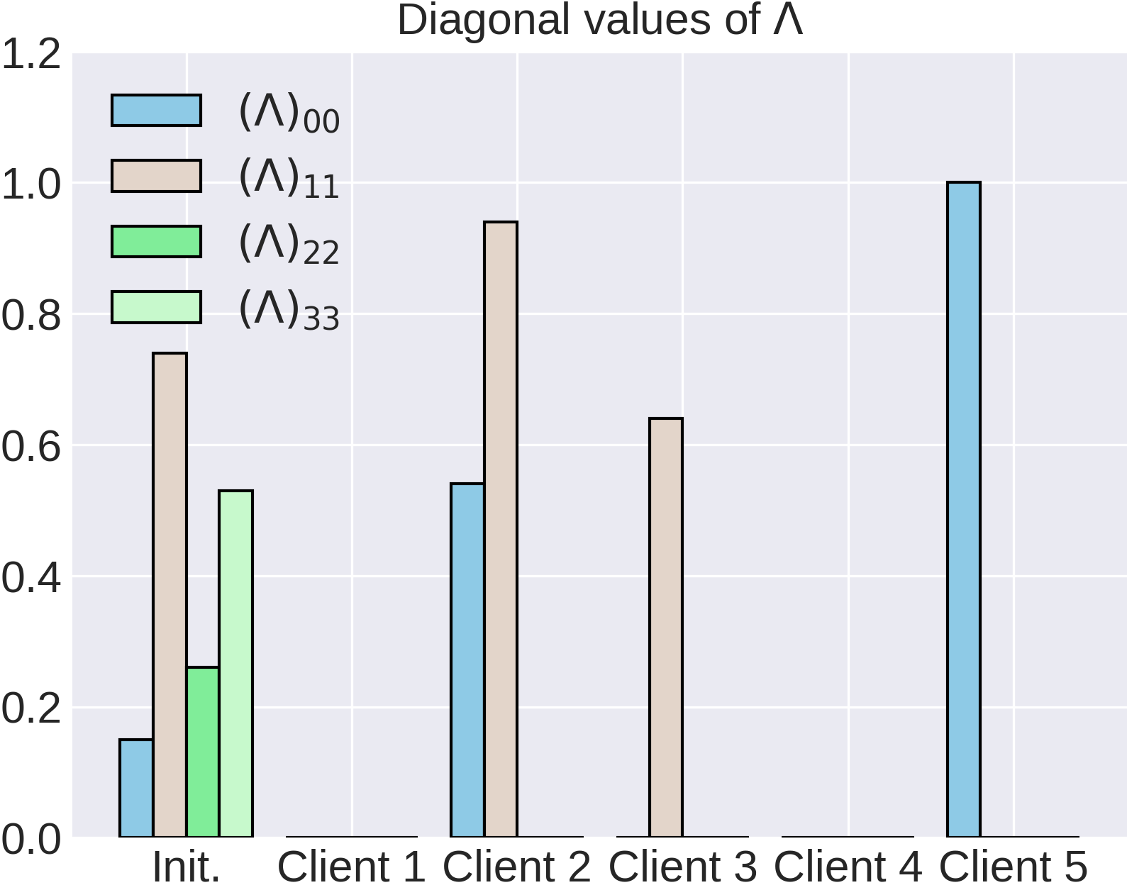
Impact of . We evaluate the impacts of learning by comparing the the performance of Learn2pFed achieved with and without learning in Setting 1 in Table I. We find that learning greatly improves performance. Specifically, the averaged RMSE is decreased from 0.0026 to 0.0002, a reduction. In addition, we analyze the learned in Fig 3. Notably, a 0 value of indicates the respective local parameters should adapt primarily to local data rather than actively participating in federated collaboration. From Fig 3, we see that the element of the matrix for all clients, which are consistent with our expectation since varies across clients in Setting 1 and thus should be learned locally. Besides, it also suggests that (in the ground-truth objective function) need to be learned locally since . Overall, these findings highlight the importance of learning in our Learn2pFed algorithm and demonstrate its ability to adapt to the characteristics of the underlying local data distribution.
Impact of the Number of Layers on Convergence. Fig. 7 in the supplemental materials shows the convergence of Learn2pFed in synthetic data w.r.t. three personalized settings mentioned above. It demonstrates that the deeper network, which unrolls more iterations of the ADMM, leads to faster convergence and more accurate solutions. Unless specified, we set for the subsequent experiments.
V-C Power Consumption Forecasting
Dataset and Federated Settings. We use the dataset Electricity Consuming Load [50] (ECL222https://archive.ics.uci.edu/ml/datasets/ElectricityLoadDiagrams20112014) for electical load forecasting, which includes power consumption records (Kwh) for over 300 clients from 2011 to 2014. After data pre-processing, there are 313 candidate clients, each with 105216 records. We perform experiments following two personalized FL settings: a) Setting 1 of full client participation scenario: we select clients that have the most distinct properties, which are distinguished by using t-SNE technique [51]. b) Setting 2 of partial client participation scenario: we randomly sample clients of over 300 clients to participate at each FL round. In both cases, we split the local data of each selected client into train and test subsets in a ratio of 9:1.
Results and Analysis. We conduct five independent trials and report the averaged RMSE results evaluated on the testing dataset in Table III. From the table, we see that different from the results in regression simulation task, optimization-based methods, including pFedMe [13] and lp_proj [15], fail to perform well in such real-world complicated datasets and require large tuning efforts. In contrast, Learn2pFed still outperforms the other approaches with lower RMSEs. Additionally, we provide visualizations of the prediction results for both participating and non-participating clients in the supplemental materials to verify the performance of the proposed Learn2pFed.
V-D Image Classification
Dataset and Federated Settings. We use two classical image classification datasets in FL, CIFAR-10 [30] and Fashion-MNIST (FMNIST) [29] in two personalized settings:
-
•
1) we consider full client participation with clients using the Dirichlet distribution [52] with argument , where a smaller indicates the greater heterogeneity among the clients.
-
•
2) we consider partial client participation in order to follow the convention in federated learning literature, e.g., in Ditto and FedRep. Specifically, we conduct experiments with 100 clients, and their data are generated according to the Dirichlet distribution with parameters . In each FL round, 10 clients are randomly selected for participation.
We further split the local data into training and testing sets at the ratio of 8:2 in both settings. In order to leverage the powerful representation capabilities of the deep neural network, we use the features extracted from the second-to-last layer of a CNN as the input of Learn2pFed. As a result, Learn2pFed aims to linearly estimate the last fully-connected layer. Then, we jointly train the CNN and Learn2pFed with only the latter involved in FL communication.
Results and Analysis. 1) Table IV shows that our proposed Learn2pFed consistently outperforms baselines across different datasets and different levels of data heterogeneity, indicating the effectiveness of learning to determine which parts of parameters for federated collaboration. Besides, Learn2pFed demonstrates enhanced performance in the presence of increased data heterogeneity. Further experimental results are provided in the supplemental materials. 2) We observe that the performances of some previous optimization-based personalized FL methods drop significantly from Table IV as the number of clients increases. The reason for this is about the intricate selection hyper-parameters, which in contrast, demonstrating the importance of dynamically determining the participation degree of local parameters in federated collaboration as our method does. 3) Fig. 4 shows the communication cost per-epoch (KB) and accuracy of several representative methods in CIFAR-10 with 10 clients and . Combined with results in Table IV, we see that our proposed Learn2pFed achieves the highest performance with minor communication cost, striking a great trade-off between communication cost and accuracy. This reveals another valuable property of our proposed Learn2pFed that it not only achieves pleasant accuracy, but also helps relieve communication cost. This reduction is attributed to Learn2pFed specifically replacing only the linear layers of the CNN model during federation, effectively minimizing communication overhead. Specifically, Learn2pFed achieves 93.45% reduction of communication cost, but outperforms FedAvg by 20% in accuracy.
| Settings | 10 clients | 100 clients | Comm. cost (KB) | |||||||
|---|---|---|---|---|---|---|---|---|---|---|
| Dataset | CIFAR-10 | FMNIST | CIFAR-10 | FMNIST | CIFAR-10 | FMNIST | ||||
| 0.1 | 0.5 | 0.1 | 0.5 | 0.1 | 0.5 | 0.1 | 0.5 | - | - | |
| Local-Only | 85.60 | 57.82 | 92.26 | 87.95 | 71.25 | 50.43 | 92.20 | 87.46 | 0 | 0 |
| FedAvg | 30.05 | 31.01 | 76.04 | 77.87 | 30.69 | 40.37 | 84.86 | 83.24 | 62.01 | 10.29 |
| FedProx | 41.68 | 52.54 | 80.42 | 86.19 | 52.56 | 48.22 | 90.84 | 87.13 | 62.01 | 10.29 |
| FedPer | 89.12 | 66.84 | 96.55 | 91.67 | 84.08 | 64.10 | 97.54 | 90.88 | 61.16 | 5.28 |
| FedRep | 86.56 | 62.39 | 96.03 | 88.72 | 84.81 | 60.27 | 96.60 | 90.11 | 61.16 | 5.28 |
| pFedMe | 90.31 | 65.19 | 97.48 | 92.86 | 83.11 | 51.07 | 98.15 | 88.56 | 62.01 | 10.29 |
| Ditto | 87.30 | 64.72 | 96.57 | 90.34 | 83.60 | 54.87 | 97.23 | 89.24 | 62.01 | 10.29 |
| CFL | 87.35 | 64.29 | 96.89 | 90.31 | 88.15 | 51.90 | 95.48 | 89.60 | 62.01 | 10.29 |
| kNN-Per | 88.47 | 64.28 | 97.64 | 90.09 | 74.69 | 61.74 | 92.13 | 88.82 | 62.01 | 10.29 |
| Learn2pFed | 90.71 | 71.02 | 98.06 | 94.09 | 89.45 | 71.64 | 98.97 | 91.99 | 4.06 | 4.06 |

Impact of layers where Learn2pFed starts in CIFAR-10. We conduct an ablation study on the selection of features extracted from the layer before the specific fc layers as inputs to Learn2pFed in CIFAR-10 (), i.e., where Learn2pFed starts. Table V shows the quantitative results. When Learn2pFed starts from the first fully-connected layer, the shared ratio increases significantly because the basic CNN’s parameter quantity primarily concentrates on the first fc layer. For this reason, our method may not always demonstrate a significant ability to reduce communication costs when starting at different layers. However, it does not impact much on the accuracy (see in Fig. 5).
| fully-connected layers | local | shared | ||
|---|---|---|---|---|
| first | second | third | parameters | ratio |
| [400,120] | [120,84] | [84,10] | (KB) | (%) |
| ✓ | 61.14 | 14.72 | ||
| ✓ | 50.99 | 17.65 | ||
| ✓ | 2.87 | 313.58 | ||

Discussions on Resource Usage. We present the memory and computation costs in CIFAR10 classification in Table VI, comparing them to those of FedAvg. Due to the replacement of the last few linear layers of the network with Learn2pFed in the classification task, we significantly cut memory usage by 88.82% (with feature extractor) and 93.13% (without feature extractor). Additionally, there is a 9.04% reduction in floating-point operations (FLOPs). That is, despite the reduction in resource usage, our performance has shown a notable improvement, demonstrating the effectiveness of our approach.
| Memory (KB) | FLOPs (M) | ||
|---|---|---|---|
| Feature Extractor | Linear layers | ||
| FedAvg | 2.87 | 59.13 | 0.6517 |
| Learn2pFed | 2.87 | 4.06 | 0.5928 |
VI Conclusion
We introduce Learn2pFed, a novel framework for personalized federated learning through algorithm unrolling. Our framework tackles the challenge of learning hyper-parameters that are typically unlearnable in the optimization process. By allowing the learnable parameters to determine the participation of local models in federated learning, we enhance adaptability of personalized FL methods. Extensive experiments on synthetic, time-series, and natural image datasets demonstrate the superior performance of Learn2pFed. Furthermore, as the unrolling-based framework, it holds potential for application in various scenarios in personalized FL approaches.
Learn2pFed focuses on dynamically determining the local parameters that should participate in the federated collaboration, but a limitation arises in its ability to explain the physical meaning of those parameters selected byLearn2pFed. We are intrigued by the potential insights it may offer for model compression or data selection and aim to explore this further in future work.
References
- [1] B. McMahan, E. Moore, D. Ramage, S. Hampson, and B. A. y Arcas, “Communication-efficient learning of deep networks from decentralized data,” in Artificial intelligence and statistics. PMLR, 2017, pp. 1273–1282.
- [2] G. Long, Y. Tan, J. Jiang, and C. Zhang, Federated Learning for Open Banking. Cham: Springer International Publishing, 2020, pp. 240–254.
- [3] D. C. Nguyen, Q.-V. Pham, P. N. Pathirana, M. Ding, A. Seneviratne, Z. Lin, O. Dobre, and W.-J. Hwang, “Federated learning for smart healthcare: A survey,” ACM Computing Surveys (CSUR), vol. 55, no. 3, pp. 1–37, 2022.
- [4] Z. Zheng, Y. Zhou, Y. Sun, Z. Wang, B. Liu, and K. Li, “Applications of federated learning in smart cities: recent advances, taxonomy, and open challenges,” Connection Science, vol. 34, no. 1, pp. 1–28, 2022.
- [5] L. Zhang, G. Gao, and H. Zhang, “Spatial-temporal federated learning for lifelong person re-identification on distributed edges,” IEEE Transactions on Circuits and Systems for Video Technology, pp. 1–1, 2023.
- [6] J. Wang, Q. Liu, H. Liang, G. Joshi, and H. V. Poor, “Tackling the objective inconsistency problem in heterogeneous federated optimization,” Advances in neural information processing systems, vol. 33, pp. 7611–7623, 2020.
- [7] P. Kairouz, H. B. McMahan, B. Avent, A. Bellet, M. Bennis, A. N. Bhagoji, K. Bonawitz, Z. Charles, G. Cormode, R. Cummings et al., “Advances and open problems in federated learning,” Foundations and Trends® in Machine Learning, vol. 14, no. 1–2, pp. 1–210, 2021.
- [8] S. AbdulRahman, H. Tout, H. Ould-Slimane, A. Mourad, C. Talhi, and M. Guizani, “A survey on federated learning: The journey from centralized to distributed on-site learning and beyond,” IEEE Internet of Things Journal, vol. 8, no. 7, pp. 5476–5497, 2020.
- [9] S. P. Karimireddy, S. Kale, M. Mohri, S. Reddi, S. Stich, and A. T. Suresh, “SCAFFOLD: Stochastic controlled averaging for federated learning,” in International conference on machine learning. PMLR, 2020, pp. 5132–5143.
- [10] A. Z. Tan, H. Yu, L. Cui, and Q. Yang, “Towards personalized federated learning,” IEEE Transactions on Neural Networks and Learning Systems, pp. 1–17, 2022.
- [11] V. Kulkarni, M. Kulkarni, and A. Pant, “Survey of personalization techniques for federated learning,” in 2020 Fourth World Conference on Smart Trends in Systems, Security and Sustainability (WorldS4). IEEE, 2020, pp. 794–797.
- [12] T. Li, A. K. Sahu, M. Zaheer, M. Sanjabi, A. Talwalkar, and V. Smith, “Federated optimization in heterogeneous networks,” Proceedings of Machine Learning and Systems, vol. 2, pp. 429–450, 2020.
- [13] C. T Dinh, N. Tran, and J. Nguyen, “Personalized federated learning with moreau envelopes,” Advances in Neural Information Processing Systems, vol. 33, pp. 21 394–21 405, 2020.
- [14] T. Li, S. Hu, A. Beirami, and V. Smith, “Ditto: Fair and robust federated learning through personalization,” in Proceedings of the 38th International Conference on Machine Learning, ser. Proceedings of Machine Learning Research, vol. 139. PMLR, 18–24 Jul 2021, pp. 6357–6368.
- [15] S. Lin, Y. Han, X. Li, and Z. Zhang, “Personalized federated learning towards communication efficiency, robustness and fairness,” Advances in Neural Information Processing Systems, 2022.
- [16] A. Fallah, A. Mokhtari, and A. Ozdaglar, “Personalized federated learning with theoretical guarantees: A model-agnostic meta-learning approach,” Advances in Neural Information Processing Systems, vol. 33, pp. 3557–3568, 2020.
- [17] F. Sattler, K.-R. Müller, and W. Samek, “Clustered federated learning: Model-agnostic distributed multitask optimization under privacy constraints,” IEEE transactions on neural networks and learning systems, vol. 32, no. 8, pp. 3710–3722, 2020.
- [18] O. Marfoq, G. Neglia, R. Vidal, and L. Kameni, “Personalized federated learning through local memorization,” in International Conference on Machine Learning. PMLR, 2022, pp. 15 070–15 092.
- [19] A. Shamsian, A. Navon, E. Fetaya, and G. Chechik, “Personalized federated learning using hypernetworks,” in Proceedings of the 38th International Conference on Machine Learning, ser. Proceedings of Machine Learning Research, vol. 139. PMLR, 18–24 Jul 2021, pp. 9489–9502.
- [20] M. G. Arivazhagan, V. Aggarwal, A. K. Singh, and S. Choudhary, “Federated learning with personalization layers,” arXiv preprint arXiv:1912.00818, 2019.
- [21] L. Collins, H. Hassani, A. Mokhtari, and S. Shakkottai, “Exploiting shared representations for personalized federated learning,” in Proceedings of the 38th International Conference on Machine Learning, ser. Proceedings of Machine Learning Research, vol. 139. PMLR, 18–24 Jul 2021, pp. 2089–2099.
- [22] K. Pillutla, K. Malik, A.-R. Mohamed, M. Rabbat, M. Sanjabi, and L. Xiao, “Federated learning with partial model personalization,” in Proceedings of the 39th International Conference on Machine Learning, ser. Proceedings of Machine Learning Research, vol. 162. PMLR, 17–23 Jul 2022, pp. 17 716–17 758.
- [23] K. Singhal, H. Sidahmed, Z. Garrett, S. Wu, J. Rush, and S. Prakash, “Federated reconstruction: Partially local federated learning,” Advances in Neural Information Processing Systems, vol. 34, pp. 11 220–11 232, 2021.
- [24] G. Sun, M. Mendieta, J. Luo, S. Wu, and C. Chen, “FedPerfix: Towards partial model personalization of vision transformers in federated learning,” in Proceedings of the IEEE/CVF International Conference on Computer Vision, 2023, pp. 4988–4998.
- [25] Z. Jiang, Y. Xu, H. Xu, Z. Wang, C. Qiao, and Y. Zhao, “FedMP: Federated learning through adaptive model pruning in heterogeneous edge computing,” in 2022 IEEE 38th International Conference on Data Engineering (ICDE). IEEE, 2022, pp. 767–779.
- [26] B. Sun, H. Huo, Y. Yang, and B. Bai, “PartialFed: Cross-domain personalized federated learning via partial initialization,” Advances in Neural Information Processing Systems, vol. 34, pp. 23 309–23 320, 2021.
- [27] E. Diao, J. Ding, and V. Tarokh, “HeteroFL: Computation and communication efficient federated learning for heterogeneous clients,” in International Conference on Learning Representations, 2021.
- [28] B. Isik, F. Pase, D. Gunduz, T. Weissman, and Z. Michele, “Sparse random networks for communication-efficient federated learning,” in The Eleventh International Conference on Learning Representations, 2023.
- [29] H. Xiao, K. Rasul, and R. Vollgraf, “Fashion-MNIST: a novel image dataset for benchmarking machine learning algorithms,” arXiv preprint arXiv:1708.07747, 2017.
- [30] A. Krizhevsky, G. Hinton et al., “Learning multiple layers of features from tiny images,” Technical report, 2009.
- [31] D. Li and J. Wang, “FedMD: Heterogenous federated learning via model distillation,” arXiv preprint arXiv:1910.03581, 2019.
- [32] X. Liu, W. Xi, W. Li, D. Xu, G. Bai, and J. Zhao, “Co-mda: Federated multisource domain adaptation on black-box models,” IEEE Transactions on Circuits and Systems for Video Technology, vol. 33, no. 12, pp. 7658–7670, 2023.
- [33] V. Monga, Y. Li, and Y. C. Eldar, “Algorithm unrolling: Interpretable, efficient deep learning for signal and image processing,” IEEE Signal Processing Magazine, vol. 38, no. 2, pp. 18–44, 2021.
- [34] A. Beck and M. Teboulle, “A fast iterative shrinkage-thresholding algorithm for linear inverse problems,” SIAM journal on imaging sciences, vol. 2, no. 1, pp. 183–202, 2009.
- [35] S. Boyd, N. Parikh, E. Chu, B. Peleato, and J. Eckstein, “Distributed optimization and statistical learning via the alternating direction method of multipliers,” Foundations and Trends® in Machine Learning, vol. 3, no. 1, pp. 1–122, 2011.
- [36] K. Gregor and Y. LeCun, “Learning fast approximations of sparse coding,” in Proceedings of the 27th international conference on international conference on machine learning, 2010, pp. 399–406.
- [37] Y. Yang, J. Sun, H. Li, and Z. Xu, “ADMM-CSNet: A deep learning approach for image compressive sensing,” IEEE transactions on pattern analysis and machine intelligence, vol. 42, no. 3, pp. 521–538, 2018.
- [38] Z. Zhao, S. Xu, J. Zhang, C. Liang, C. Zhang, and J. Liu, “Efficient and model-based infrared and visible image fusion via algorithm unrolling,” IEEE Transactions on Circuits and Systems for Video Technology, vol. 32, no. 3, pp. 1186–1196, 2022.
- [39] S. Chen, Y. C. Eldar, and L. Zhao, “Graph unrolling networks: Interpretable neural networks for graph signal denoising,” IEEE Transactions on Signal Processing, vol. 69, pp. 3699–3713, 2021.
- [40] H. Vu, G. Cheung, and Y. C. Eldar, “Unrolling of deep graph total variation for image denoising,” in ICASSP 2021 - 2021 IEEE International Conference on Acoustics, Speech and Signal Processing (ICASSP), 2021, pp. 2050–2054.
- [41] Y. Li, M. Tofighi, J. Geng, V. Monga, and Y. C. Eldar, “Efficient and interpretable deep blind image deblurring via algorithm unrolling,” IEEE Transactions on Computational Imaging, vol. 6, pp. 666–681, 2020.
- [42] M. Hong, Z.-Q. Luo, and M. Razaviyayn, “Convergence analysis of alternating direction method of multipliers for a family of nonconvex problems,” SIAM Journal on Optimization, vol. 26, no. 1, pp. 337–364, 2016.
- [43] M. Hong and Z.-Q. Luo, “On the linear convergence of the alternating direction method of multipliers,” Mathematical Programming, vol. 162, no. 1-2, pp. 165–199, 2017.
- [44] Y. LeCun, Y. Bengio, and G. Hinton, “Deep learning,” nature, vol. 521, no. 7553, pp. 436–444, 2015.
- [45] H. Robbins and S. Monro, “A stochastic approximation method,” The annals of mathematical statistics, pp. 400–407, 1951.
- [46] B. Fehrman, B. Gess, and A. Jentzen, “Convergence rates for the stochastic gradient descent method for non-convex objective functions,” The Journal of Machine Learning Research, vol. 21, no. 1, pp. 5354–5401, 2020.
- [47] M. Fredrikson, S. Jha, and T. Ristenpart, “Model inversion attacks that exploit confidence information and basic countermeasures,” in Proceedings of the 22nd ACM SIGSAC conference on computer and communications security, 2015, pp. 1322–1333.
- [48] R. Shokri, M. Stronati, C. Song, and V. Shmatikov, “Membership inference attacks against machine learning models,” in 2017 IEEE symposium on security and privacy (SP). IEEE, 2017, pp. 3–18.
- [49] Y. Yu, X. Si, C. Hu, and J. Zhang, “A review of recurrent neural networks: LSTM cells and network architectures,” Neural computation, vol. 31, no. 7, pp. 1235–1270, 2019.
- [50] G. Lai, W.-C. Chang, Y. Yang, and H. Liu, “Modeling long-and short-term temporal patterns with deep neural networks,” in The 41st International ACM SIGIR Conference on Research & Development in Information Retrieval, ser. SIGIR ’18. New York, NY, USA: Association for Computing Machinery, 2018, pp. 95–104.
- [51] L. Van der Maaten and G. Hinton, “Visualizing data using t-SNE.” Journal of machine learning research, vol. 9, no. 11, 2008.
- [52] M. Yurochkin, M. Agarwal, S. Ghosh, K. Greenewald, N. Hoang, and Y. Khazaeni, “Bayesian nonparametric federated learning of neural networks,” in International conference on machine learning. PMLR, 2019, pp. 7252–7261.
