Are the dynamics of wall turbulence in minimal channels and larger domain channels equivalent? A graph-theoretic approach

Ahmed Elnahhas¹ Emma Lenz² Parviz Moin¹ Adrián Lozano-Durán³ and H. Jane Bae² ¹ Center for Turbulence Research, Stanford University, Stanford CA, 94305 USA ² Graduate Aerospace Laboratories, California Institute of Technology, Pasadena CA, 91125 USA ³ Department of Aeronautics & Astronautics, Massachusetts Institute of Technology, Cambridge MA, 02139 USA ahmed97@stanford.edu

Abstract

This work proposes two algorithmic approaches to extract critical dynamical mechanisms in wall-bounded turbulence with minimum human bias. In both approaches, multiple types of coherent structures are spatiotemporally tracked, resulting in a complex multilayer network. Network motif analysis, i.e., extracting dominant non-random elemental patterns within these networks, is used to identify the most dominant dynamical mechanisms. Both approaches, combined with network motif analysis, are used to answer whether the main dynamical mechanisms of a minimal flow unit (MFU) and a larger unconstrained channel flow, labeled a full channel (FC), at $Re_{\tau}\approx 180$ , are equivalent. The first approach tracks traditional coherent structures defined as low- and high-speed streaks, ejections, and sweeps. It is found that the roll-streak pairing, consistent with the current understanding of self-sustaining processes, is the most significant and simplest dynamical mechanism in both flows. However, the MFU has a timescale for this mechanism that is approximately $2.83$ times slower than that of the FC. In the second approach, we use semi-Lagrangian wavepackets and define coherent structures from their energetic streak, roll, and small-scale phase space. This method also shows similar motifs for both the MFU and FC. It indicates that, on average, the most dominant phase-space motifs are similar between the two flows, with the significant events taking place approximately $2.21$ times slower in the MFU than in the FC. This value is more consistent with the implied timescale ratio of only the slow speed streaks taking part in the roll-streak pairing extracted using the first multi-type spatiotemporal approach, which is approximately $2.17$ slower in the MFU than the FC.

1 Introduction

It has long been hypothesized that wall-bounded turbulence can be decomposed into a set of coherent structures that coexist and interact [1]. This concept can be interpreted kinematically by synthesizing the turbulent flow field as a superposition of building block eddies; the attached eddy model (AEM) adopts this approach for high- $Re_{\tau}$ flows using a hierarchy of eddies scaling with distance from the wall [2, 3]. A more comprehensive model would account for the dynamics of the building block eddies, both in isolation as well as for their interactions. The most famous dynamic coherent structure model of wall-bounded turbulence is the roll-streak self-sustaining process (SSP) [4, 5, 6, 7, 8, 9, 10, 11, 12]. This SSP is primarily extracted from simulations of minimal flow units (MFU) at low $Re_{\tau}$ , which isolate a single scale of wall-bounded turbulence, as well as a single instance of the SSP at a time by enforcing severe periodicity [4, 5, 6, 12]. These MFU simulations have also been extended to larger scales by isolating structures in the logarithmic region of the flow where similar dynamical cycles were observed [7, 8, 9, 10, 11]. Taking the AEM, one can theorize that a “dynamic”-AEM can be constructed based on the findings from MFUs of the buffer and logarithmic regions of the flow by superposing SSPs at each scale of motion and neglecting strong interscale interactions. However, recent experimental observations of inner/outer modulation and large-scale streak aggregation suggest more to the story [13, 14, 15, 16]. Hence, a few questions immediately arise concerning the current understanding of wall-bounded turbulence: Are the dynamics extracted from MFUs relevant to wall-bounded turbulent flows in large unbounded domains at the same $Re_{\tau}$ ? Or do interactions between different instances of SSPs heavily influence each other, perhaps altering their timescales? Are other, possibly dominant, dynamic cycles suppressed in the artificially restricted domains of MFUs? Finally, what is the importance of interscale interactions of different-sized SSPs at larger $Re_{\tau}$ ? To understand the dynamical interactions amongst the same scales of motion and inter-scale, we need to find a systematic and algorithmic way to extract and study these dynamics. In this study, we propose such a framework and apply it first to study whether the dynamics of the MFU exist unaltered in large domain channel simulations, henceforth referred to as full channels (FC), at $Re_{\tau}=180$ , or not.

Recently, coherent structure identification and temporal tracking algorithms have been developed to understand the basic dynamical properties of select eddy definitions, such as momentum-carrying structures, velocity streaks, and energy-containing eddies [17, 18, 19, 20]. These algorithms are based on spatial and temporal clustering of grid points that satisfy certain thresholding and proximity criteria. The result is a directed graph where the nodes represent the coherent structures, and the edges represent temporal connections between the structures. Therefore, advanced graph processing tools can extract information about these coherent structures’ spatiotemporal properties. Extending the clustering and tracking algorithms to track several definitions of eddies simultaneously, along with the interconnections between eddy types, results in a higher dimensional graph, where the eddy type acts as the new dimension, called a multilayered network [21, 22]. We use network motifs and graphlet search algorithms [23, 24] to analyze and compare dynamically significant patterns extracted from the buffer layer MFU and large domain channel flows.

A network motif of a complex network is a pattern occurring at a significantly higher frequency than in a random network of the same size [23]. Network motifs have been identified in various biological networks, such as those responsible for gene expression and neuronal cell interactions [25]. They have also been identified in larger-scale ecological and engineering networks [23]. Since our directed multilayer network has time embedded in its construction, detecting motifs accounts for the most significant dynamical patterns between eddies of various types directly. Figure 1(a) illustrates the proposed approach. Each node in the network represents the full spatiotemporal history of a coherent structure, and the edges represent the interactions between two coherent structures at some point during their evolution. In the context of the current question, finding the most dominant interaction pattern compared to a set of random networks helps us isolate the key dynamical mechanism in both the FC and the MFU and compare their similarity. Applications of network analysis to fluid flow are only recent phenomena [18, 26, 27, 28, 29, 30, 31, 32, 33, 34], and applications to the study of the dynamics of coherent structures have not been attempted in fully developed wall-bounded turbulent flows. The results of this spatiotemporal approach are supplemented with motifs extracted from an energetic phase-space constructed using semi-Lagrangian wavepackets illustrated in figure 1(b).

The rest of the paper is organized as follows. Section 2 describes the datasets utilized to perform the analysis. In section 3, the multi-type coherent structure tracking and motif detection algorithms are described, and the results of their application to the MFU and the FC at $Re_{\tau}=180$ are discussed. In section 4, the semi-Lagrangian wavepackets and phase-space temporal motif analysis approach is explained, and the results of applying it to the same datasets are discussed. Finally, conclusions and future work are presented in section 5.

2 Simulation details

Let $u_{\tau}$ and $\nu$ denote the flow’s friction velocity and kinematic viscosity, respectively. The two flows analyzed are direct numerical simulations (DNS) of an MFU and an FC inside a channel of half-height $\delta$ . The friction Reynolds number for both flows is $Re_{\tau}\equiv\delta u_{\tau}/\nu\approx 180$ . In this flow, $x$ , $y$ , and $z$ are the streamwise, wall-normal, and spanwise directions, respectively, corresponding to their respective mean and fluctuating velocities $U$ and $u$ , $V$ and $v$ , and $W$ and $w$ . The domain of the MFU has a size of $\{0.564\pi\times 2\times 0.282\pi\}\delta$ , and that of the FC has a size of $\{8\pi\times 2\times 3\pi\}\delta$ . The resolution in inner units of both simulations are $\{\Delta x^{+},\Delta y^{+}_{min},\Delta y^{+}_{max},\Delta z^{+}\}=\{6.05,0.17,7.52,6.05\}$ , which is consistent with prior DNS simulations. Flow fields are stored every $\Delta t^{+}\approx 1$ for $T^{+}=2000$ and $T^{+}=25000$ inner time units for the FC and MFU, respectively. These correspond to approximately $11\delta/u_{\tau}$ and $135\delta/u_{\tau}$ , respectively.

3 Multi-type spatiotemporal coherent-structure tracking and motif detection

3.1 Multilayer network generation

The multi-type coherent-structure tracking algorithm is a three-step process, schematically illustrated in figure 1(a):

Step 1: In this work, the eddies considered are the low- and high-speed streaks and wall-normal streamwise momentum flux eddies, namely ejections and sweeps, interchangeably referred to as Q2 and Q4, respectively [17, 20]. At each time instant, each of these eddies is defined as the set of connected points in space, $\Omega$ , satisfying the following inequalities

\big{\{}(x,y,z):|uv|>\alpha_{uv}u^{\prime}(y)v^{\prime}(y)\quad\&\quad\begin{cases}\bigg{(}\frac{\int_{\Omega}u~{}dV_{\Omega}}{\int_{\Omega}dV_{\Omega}}<0\bigg{)}~{}\&~{}\bigg{(}\frac{\int_{\Omega}v~{}dV_{\Omega}}{\int_{\Omega}dV_{\Omega}}>0\bigg{)}\bigg{\}}\implies\mathrm{Ejections~{}(Q2)}\\[10.0pt] \bigg{(}\frac{\int_{\Omega}u~{}dV_{\Omega}}{\int_{\Omega}dV_{\Omega}}>0\bigg{)}~{}\&~{}\bigg{(}\frac{\int_{\Omega}v~{}dV_{\Omega}}{\int_{\Omega}dV_{\Omega}}<0\bigg{)}\bigg{\}}\implies\mathrm{Sweeps~{}(Q4)}\end{cases}\mathrm{,}

(1)

\big{\{}(x,y,z):\sqrt{u^{2}+w^{2}}>\alpha_{str}u^{\prime}(y)\quad\&\quad\begin{cases}u<0\big{\}}\implies\mathrm{Slow~{}Streak}\\ u>0\big{\}}\implies\mathrm{Fast~{}Streak}\end{cases}{,}

(2)

where $u^{\prime}(y)$ and $v^{\prime}(y)$ are the root-mean-squared streamwise and wall-normal velocity fluctuations extracted from the corresponding simulation, i.e., the MFU and the FC, $\alpha_{\{uv,str\}}$ are scaling coefficients for the thresholds, and $V_{\Omega}$ is the physical volume associated with the set of points, $\Omega$ . The clustering process is known to have a percolation crisis, and we use the values $\{\alpha_{\tau},\alpha_{str}\}=\{1.30,1.75\}$ , which maximize the number of clusters identified per timestep on average. Each region, $\Omega$ , is labeled as a coherent structure at some instant in its evolution. Once subdivided into these four sets, contiguous time snapshots construct their temporal evolution.

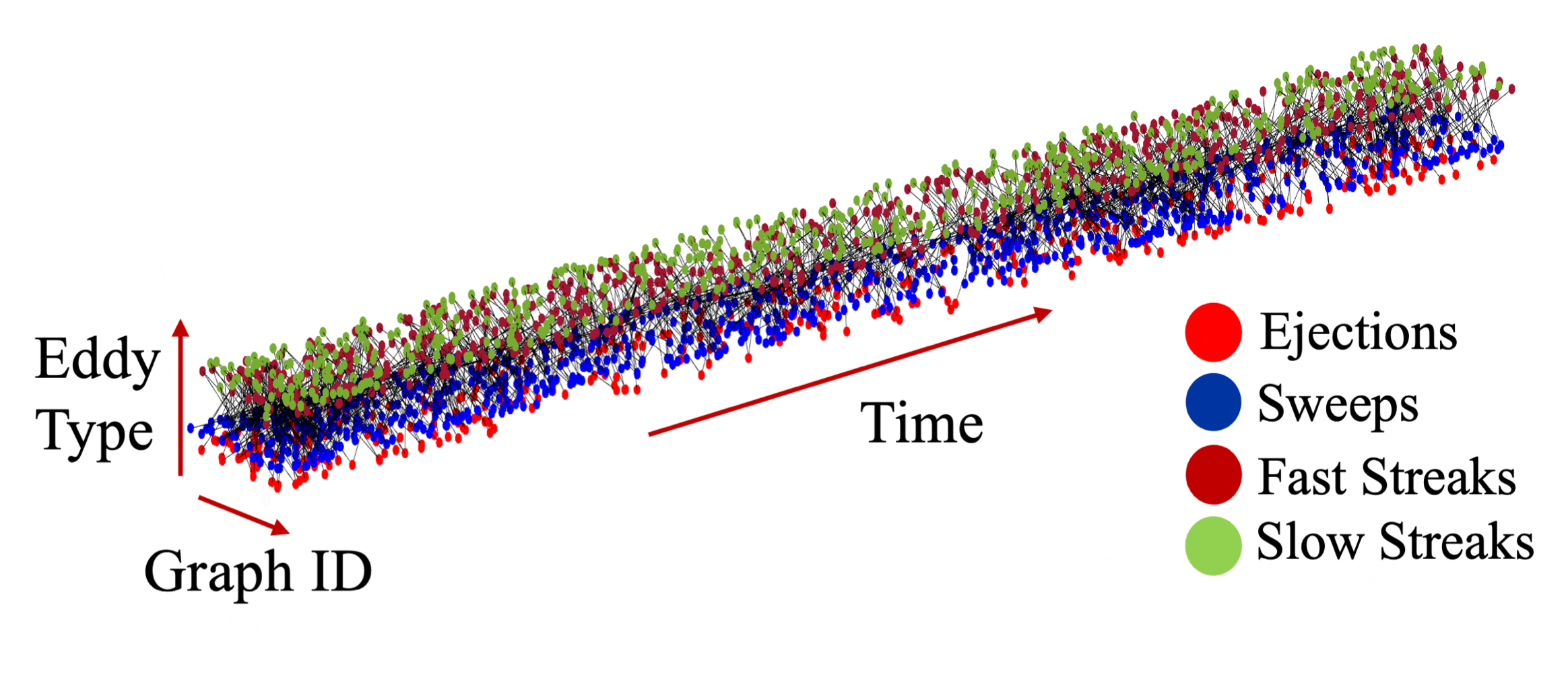
Step 2: The details of the structure tracking in time are described in [18]. In summary, object volumetric overlap between timesteps is used to construct a graph with edges representing connections in time and objects at different time steps representing nodes. While previously this was done for only a single type of object, this procedure is repeated $N^{2}$ times where $N$ is the number of eddy types. The graph is first clustered into branches, which are the links between objects that mutually experience the least relative change from one timestep to the next.

Step 3: The branches are then further partitioned to generate subgraphs or trees, which are collections of branches that interact in a “primary” way. We define a primary branch connection using the relative overlap metric from branch $i$ to $j$ of the same eddy type and vice versa, which is defined as follows

O_{i\rightarrow j}=\frac{\int V_{i}\cap V_{j}dt_{i}}{\int V_{i}dt_{i}}\quad\text{and}\quad O_{j\rightarrow i}=\frac{\int V_{j}\cap V_{i}dt_{j}}{\int V_{j}dt_{j}}\text{,}

(3)

where the integration is over the lifetime of the source branch and $V_{i}$ is the volume of a branch at a given time across its lifetime. The intersecting volume is computed at the same absolute time for both branches. The branch link $j$ to branch $i$ with the highest overlap metric is considered the primary branch in the positive or negative time directions. If two branches are each other’s primary links, they are clustered into a subgraph or tree. This process is applied recursively, and each resulting tree is subsequently referred to as a spatiotemporal eddy. An illustration of the partitioning when two branches do not point to each other as primary branch connections is represented with the crossed orange lines in figure 1(a).

During step 2 and step 3 of the process, the physical connections between eddies of different types are transferred from single-time connections at the end of step 1 to connections between branches and, finally, trees at the end of steps 2 and 3, respectively. This results in a large, complex, multilayered network that encodes spatiotemporal interactions between eddies of the same type and those between eddies of different types. These intertype connections are represented with green lines in the schematic illustration of figure 1(a).

After the three-step process, many of the spatiotemporal eddies are small structures existing in the center of the channel, which, if tracked, result in an overly large/complex multilayer network. To ease the subsequent analysis, we limit ourselves to interactions between attached eddies that live for a minimal amount of time, i.e., those who, at some point during their lifetime, had a minimal wall-normal height (on either wall) of $y^{+}_{min}<20$ [18, 20], and have lived for longer than $T^{+}_{life}=20$ . Furthermore, they must have interacted with another attached eddy during their lifetime. The volumes occupied by the ejections, sweeps, slow, and fast streaks that satisfy these criteria and subsets of them in both the MFU and the FC are presented in table 3.1. The applied criteria only restrict the minority of the attached eddies by volume, approximately $11.5-17.5\%$ , from participating in the subsequent motif analysis. Figure 2(a) showcases the result of the step 3 partitioning of branches into trees using the overlap metric for attached eddies, where the size of the trees in terms of branches is exponentially decaying, and no single tree contains more than $\mathcal{O}(10)$ branches. Given this partitioning, figure 2(b) shows a subset of the multilayer network that emerges due to all the interactions of attached spatiotemporal ejections, sweeps, and slow and fast streaks in the FC where each dot contains within it the entirety of the detailed spatiotemporal evolution of each of the spatiotemporal eddies.

[Uncaptioned image] — Table 1: The average percentage of the domain’s volume occupied by certain types of eddies that satisfy particular criteria in both the full channel and minimal flow unit. $\mathcal{A}:{y_{min}^{+}<20}$ . $\mathcal{T}:{T_{life}^{+}>20}$ . $\mathcal{I}:\text{Interaction with another $\mathcal{A}-$\text{valid eddy}}$ . $\mathcal{S}_{1}^{\{F,M\}}:\text{Involved in most significant roll-streak motif}$ . $\mathcal{F}_{2}^{M}:\text{Involved in similar motif only presented in MFU}$ . The two values for $\mathcal{S}_{1}^{M}$ and $\mathcal{F}_{2}^{M}$ eddies are averages performed over the entire temporal extent of the simulation and only over the times when constituent eddies in the motifs are alive, respectively.

\br Minimal Flow Unit			Full Channel
\mrFilter	Q2 & Q4	Streaks	Filter	Q2 & Q4	Streaks
\mr $\mathcal{A}$	5.12%	2.55%	$\mathcal{A}$	5.19%	2.43%
$\mathcal{A}~{}\&~{}\mathcal{T}$	4.90%	2.52%	$\mathcal{A}~{}\&~{}\mathcal{T}$	4.52%	2.15%
$\mathcal{A}~{}\&~{}\mathcal{T}~{}\&~{}\mathcal{I}$	4.43%	2.31%	$\mathcal{A}~{}\&~{}\mathcal{T}~{}\&~{}\mathcal{I}$	4.16%	2.10%
$\mathcal{A}~{}\&~{}\mathcal{T}~{}\&~{}\mathcal{I}~{}\&~{}\mathcal{S}^{M}_{1}$	1.09-3.87%	0.72-2.44%	$\mathcal{A}~{}\&~{}\mathcal{T}~{}\&~{}\mathcal{I}~{}\&~{}\mathcal{S}^{F}_{1}$	2.04%	1.01%
$\mathcal{A}~{}\&~{}\mathcal{T}~{}\&~{}\mathcal{I}~{}\&~{}\mathcal{F}^{M}_{2}$	2.56-4.14%	1.10-2.15%	—	—	—
\br

\mr	Significance Ordering							Frequency Ordering
\mrFC	$\mathcal{S}_{1}^{F}$	$\mathcal{S}_{2}^{F}$	$\mathcal{S}_{3}^{F}$	$\mathcal{S}_{4}^{F}$	$\mathcal{S}_{5}^{F}$	$\mathcal{S}_{6}^{F}$	$\mathcal{S}_{7}^{F}$	$\mathcal{F}_{1}^{F}$	$\mathcal{F}_{2}^{F}$	$\mathcal{F}_{3}^{F}$	$\mathcal{F}_{4}^{F}$	$\mathcal{F}_{5}^{F}$	$\mathcal{F}_{6}^{F}$
\mr $\widetilde{W}(s)$	4.71	3.76	3.50	3.47	3.13	3.04	2.56	0.13	0.13	0.13	0.13	0.13	0.13
$\mathcal{F}(s)$	0.26	0.19	0.16	0.14	0.15	0.09	0.09	7.28	7.10	6.10	4.95	3.53	3.36
\mr
\mrMFU	$\mathcal{S}_{1}^{M}$	$\mathcal{S}_{2}^{M}$	$\mathcal{S}_{3}^{M}$	$\mathcal{S}_{4}^{M}$	$\mathcal{S}_{5}^{M}$	$\mathcal{S}_{6}^{M}$	—	$\mathcal{F}_{1}^{M}$	$\mathcal{F}_{2}^{M}$	$\mathcal{F}_{3}^{M}$	$\mathcal{F}_{4}^{M}$	$\mathcal{F}_{5}^{M}$	$\mathcal{F}_{6}^{M}$
\mr $\widetilde{W}(s)$	1.54	1.30	0.83	0.79	0.73	0.38	—	0.37	0.05	0.37	0.37	0.37	0.37
$\mathcal{F}(s)$	0.72	0.47	0.34	0.35	0.14	0.10	—	15.20	8.86	8.67	3.83	3.49	3.25
\mr

\mr $\overline{T^{+}}_{life}$
\mrMotif Identifier	Minimal Flow Unit	Full Channel
\mr $\mathcal{S}_{1}^{F,M}$	601	212
\mr $\overline{u^{+}}_{adv}$
\mrEddy Type	Minimal Flow Unit	Full Channel
\mrEjections	4.50	14.07
Sweeps	11.01	14.30
Fast Streaks	9.28	11.86
Slow Streaks	6.00	13.00
\mr

\mrFC	Emergence(%)				Death(%)
\mrEddy Type	$1^{\mathrm{st}}$	$2^{\mathrm{nd}}$	$3^{\mathrm{rd}}$	$4^{\mathrm{th}}$	$1^{\mathrm{st}}$	$2^{\mathrm{nd}}$	$3^{\mathrm{rd}}$	$4^{\mathrm{th}}$
\mrEjections	14.2	20.7	24.5	40.6	35.1	27.2	21.8	15.9
Sweeps	28.8	25.3	21.6	24.3	32.8	23.2	21.9	22.1
Fast Streaks	37.6	26.1	22.1	14.2	11.4	20.1	28.8	39.7
Slow Streaks	19.4	31.8	27.9	20.9	20.7	29.5	27.5	22.3
\mrMFU	Emergence(%)				Death(%)
\mrEddy Type	$1^{\mathrm{st}}$	$2^{\mathrm{nd}}$	$3^{\mathrm{rd}}$	$4^{\mathrm{th}}$	$1^{\mathrm{st}}$	$2^{\mathrm{nd}}$	$3^{\mathrm{rd}}$	$4^{\mathrm{th}}$
\mrEjections	49.3	24.7	17.9	8.1	9.6	15.8	17.9	56.7
Sweeps	13.0	18.9	29.2	38.9	42.9	27.5	19.4	10.2
Fast Streaks	25.3	29.6	35.2	9.9	15.2	38.3	28.3	18.2
Slow Streaks	12.4	26.8	17.8	43.0	32.3	18.3	34.5	14.9
\mr

\br Minimal Flow Unit			Full Channel
\mr $s$	$\widetilde{W}(s)$	Occ.	$s$	$\widetilde{W}(s)$	Occ.
\mr $\mathbf{(0,0,1)\to(1,0,1)\to(1,0,0)}$	0.0466	79	${(0,1,1)\to(1,1,1)\to(1,1,0)}$	0.0178	910
${(0,1,0)\to(1,1,0)\to(1,0,0)}$	0.0432	283	$\mathbf{(0,0,0)\to(1,0,0)\to(1,1,0)}$	0.0167	282
$(0,0,0)\to(0,0,1)\to(1,0,1)$	0.0410	138	${(1,0,1)\to(1,1,1)\to(1,0,1)}$	0.0156	127
$(1,1,1)\to(1,1,0)\to(0,1,0)$	0.0305	89	$\mathbf{(0,0,1)\to(1,0,1)\to(1,0,0)}$	0.0153	106
$\mathbf{(0,0,0)\to(1,0,0)\to(1,1,0)}$	0.0296	261	$(0,0,1)\to(1,0,1)\to(1,1,1)$	0.0132	206
\br

Are the dynamics of wall turbulence in minimal channels and larger domain channels equivalent? A graph-theoretic approach

Abstract

1 Introduction

2 Simulation details

3 Multi-type spatiotemporal coherent-structure tracking and motif detection

3.1 Multilayer network generation

3.2 Motif detection

3.3 Results

4 Semi-Lagrangian wavepackets and phase-space temporal motifs

4.1 Defining the size of the semi-Lagrangian wavepackets

4.2 Production–dissipation trajectories and advection speed

4.3 Temporal motif of energy contained in streak, roll, and small scales

5 Conclusions

Acknowledgments

References

References

- [1] Robinson S K 1991 Coherent motions in the turbulent boundary layer Annu. Rev. Fluid Mech. 23 601–639
- [2] Townsend A A 1976 The Structure of Turbulent Shear Flow (Cambridge, UK: Cambridge University Press)
- [3] Marusic I and Monty J P 2019 Attached eddy model of wall turbulence Annu. Rev. Fluid Mech. 51 49–74
- [4] Jiménez J and Moin P 1991 The minimal flow unit in near-wall turbulence J. Fluid Mech. 225 213–240
- [5] Hamilton J M, Kim J and Waleffe F 1995 Regeneration mechanisms of near-wall turbulence structures J. Fluid Mech. 287 317–348
- [6] Jiménez J and Pinelli A 1999 The autonomous cycle of near-wall turbulence J. Fluid Mech. 389 335–359
- [7] Flores O and Jiménez J 2010 Hierarchy of minimal flow units in the logarithmic layer Phys. Fluids 22 71704
- [8] Hwang Y and Cossu C 2010 Self-sustained process at large scales in turbulent channel flow Phys. Rev. Letters 105 044505
- [9] Hwang Y and Cossu C 2011 Self-sustained processes in the logarithmic layer of turbulent channel flows Phys. Fluids 23 061702
- [10] Bae H J and Lozano-Durán A 2019 A minimal flow unit of the logarithmic layer in the absence of near-wall eddies and large scales Annu. Res. Briefs, Center for Turbulence Research, Stanford University, 247–256
- [11] Bae H J, Lozano-Durán A and McKeon B 2021 Nonlinear mechanism of the self-sustaining process in the buffer and logarithmic layer of wall-bounded flows J. Fluid Mech. 914 A3
- [12] Lozano-Durán A, Bae H J and Encinar M P 2020 Causality of energy-containing eddies in wall turbulence J. Fluid Mech. 882 A2
- [13] Hutchins N and Marusic I 2007 Evidence of very long meandering features in the logarithmic region of turbulent boundary layers J. Fluid Mech. 579 1–28
- [14] Hutchins N and Marusic I 2007 Large-scale influences in near-wall turbulence Phil. Trans. Royal Soc. A: Math. Phys. Eng. Sci. 365 647–664
- [15] Marusic I, Mathis R and Hutchins N 2010 Predictive model for wall-bounded turbulent flow Science 329 193–196
- [16] Zhou Z, Xu C X and Jiménez J 2022 Interaction between near-wall streaks and large-scale motions in turbulent channel flows J. Fluid Mech. 940 A23
- [17] Lozano-Durán A, Flores O and Jiménez J 2012 The three-dimensional structure of momentum transfer in turbulent channels J. Fluid Mech. 694 100–130
- [18] Lozano-Durán A and Jiménez J 2014 Time-resolved evolution of coherent structures in turbulent channels: characterization of eddies and cascades J. Fluid Mech. 759 432–471
- [19] Dong S, Huang Y, Yuan X and Lozano-Durán A 2020 The coherent structure of the kinetic energy transfer in shear turbulence J. Fluid Mech. 892 A22
- [20] Bae H J and Lee M 2021 Life cycle of streaks in the buffer layer of wall-bounded turbulence Phys. Rev. Fluids 6 064603
- [21] Boccaletti S, Bianconi G, Criado R, Del Genio C I, Gómez-Gardeñes J, Romance M, Sendiña-Nadal I, Wang Z and Zanin M 2014 The structure and dynamics of multilayer networks Phys. Reports 544 1–122
- [22] Kivelä M, Arenas A, Barthelemy M, Gleeson J P, Moreno Y, Porter A M and Estrada E 2014 Multilayer networks J. Comp. Networks 2 203–271
- [23] Milo R, Shen-Orr S, Itzkovitz S, Kashtan N, Chklovskii D and Alon U 2002 Network motifs: Simple building blocks of complex networks Science 298 824–827
- [24] Ribeiro P, Paredes P, Silve M E P, Aparicio D and Silva F 2021 A survey on subgraph counting ACM Comp. Surveys 54 A28
- [25] Alon U 2007 Network motifs: theory and experimental approaches Nature Rev. Gen. 8 450–461
- [26] Taira K, Nair A G and Brunton S L 2016 Network structure of two-dimensional decaying isotropic turbulence J. Fluid Mech. 795 R2
- [27] Schmid P J, García-Gutierrez A and Jiménez J 2018 Description and detection of burst events in turbulent flows J. Phys.: Conf. Ser. 1001, Third Madrid Summer School for Turbulence, 012015
- [28] Iacobello G, Scarsoglio S, Kuerten J G M and Ridolfi L 2019 Lagrangian network analysis of turbulent mixing J. Fluid Mech. 865 546–562
- [29] Krueger P S, Hahsler M, Olinick E V, Williams S H and Zharfa M 2019 Quantitative classification of vortical flows based on topological features using graph matching Proc. Royal Soc. A: Math. Phys. Eng. Sci. 475 A8
- [30] Fernex D, Noack B R and Semaan R 2021 Cluster-based network modeling: From snapshots to complex dynamical systems Science Adv. 7 5006–5022
- [31] Iacobello G, Ridolfi L and Scarsoglio S 2021 Large-to-small scale frequency modulation analysis in wall-bounded turbulence via visibility networks J. Fluid Mech. 918 A13
- [32] Li H, Fernex D, Semaan R, Tan J, Morzyński M and Noack B R 2021 Cluster-based network model J. Fluid Mech. 906 A21
- [33] Perrone D, Kuerten J G M, Ridolfi L and Scarsoglio S 2021 Network analysis of Reynolds number scaling in wall-bounded lagrangian mixing Phys. Rev. Fluids 6 124501
- [34] Taira K and Nair A G 2022 Network-based analysis of fluid flows: Progress and outlook Prog. Aero. Sci. 131 100823
- [35] Wernicke S and Rasche F FANMOD: a tool for fast network motif detection Bioinformatics. 22 1152–1153
- [36] Wernicke S Efficient detection of network motifs IEEE/ACM trans. comp. biology & bioinformatics 3 347–359
- [37] Ribeiro P and Silva F 2014 Discovering colored network motifs Complex Networks V: Proceedings of the 5th Workshop on Complex Networks 107–118
- [38] Jiménez J, Kawahara G, Simens M P, Nagata M and Shiba M 2005 Characterization of near-wall turbulence in terms of equilibrium and “bursting” solutions Phys. Fluids 17 015105
- [39] Benson A R, Gleich D F and Leskovec J 2016 Higher-order organization of complex networks Science, 353 163–166