Implied volatility (also) is path-dependent

Hervé Andrès Milliman R&D, Paris, France CERMICS, École des Ponts, INRIA, Marne-la-Vallée, France. Alexandre Boumezoued Milliman R&D, Paris, France Benjamin Jourdain CERMICS, École des Ponts, INRIA, Marne-la-Vallée, France.

Abstract

We propose a new model for the coherent forecasting of both the implied volatility surfaces and the underlying asset returns. In the spirit of Guyon and Lekeufack (2023) who are interested in the dependence of volatility indices (e.g. the VIX) on the paths of the associated equity indices (e.g. the S&P 500), we first study how implied volatility can be predicted using the past trajectory of the underlying asset price. Our empirical study reveals that a large part of the movements of the at-the-money-forward implied volatility for up to two years maturities can be explained using the past returns and their squares. Moreover, we show that up to four years of the past evolution of the underlying price should be used for the prediction and that this feedback effect gets weaker when the maturity increases. Building on this new stylized fact, we fit to historical data a parsimonious version of the SSVI parameterization (Gatheral and Jacquier, 2014) of the implied volatility surface relying on only four parameters and show that the two parameters ruling the at-the-money-forward implied volatility as a function of the maturity exhibit a path-dependent behavior with respect to the underlying asset price. Finally, we propose a model for the joint dynamics of the implied volatility surface and the underlying asset price. The latter is modelled using a variant of the path-dependent volatility model of Guyon and Lekeufack and the former is obtained by adding a feedback effect of the underlying asset price onto the two parameters ruling the at-the-money-forward implied volatility in the parsimonious SSVI parameterization and by specifying a hidden semi-Markov diffusion model for the residuals of these two parameters and the two other parameters. Thanks to this model, we are able to simulate highly realistic paths of implied volatility surfaces that are arbitrage-free.

Keywords: implied volatility modelling, SSVI, path-dependent volatility

1 Introduction

One of the many reasons of the success of the Black-Scholes model (Black and Scholes, 1973) is the existence of a one-to-one correspondence between the price $C(K,T)$ of an European call option with strike $K$ and maturity $T$ and the volatility $\sigma$ of the geometric Brownian motion modelling the dynamics of the underlying asset price $(S_{t})_{t\geq 0}$ provided that $(S_{0}-Ke^{-rT})^{+}<C(K,T)<S_{0}$ ( $r$ is the constant risk-free rate) which is guaranteed by absence of arbitrage opportunities. When this condition is satisfied, the unique parameter $\sigma$ satisfying $C_{BS}(K,T,\sigma)=C(K,T)$ , where $C_{BS}$ denotes the Black-Scholes call option price, is called the implied volatility of the call option. By the put-call parity, the implied volatility of the put option is equal to the one of the call option with same maturity and strike. Although the implied volatility does not add any new information with respect to the option price, it is commonly used to quote option prices on the markets mainly because it allows to easily compare the value of two options with different underlying assets while the option price heavily depends on the underlying asset price level, making the comparison more difficult. If the Black-Scholes model was an accurate description of financial markets, the implied volatility should be the same for all options on a given asset regardless of the maturity and the strike. The computation of the implied volatility from market option prices shows that the implied volatility actually depends on the maturity and the strike which invalidates the Black-Scholes model. The so-called implied volatility surface (IVS) $(K,T)\mapsto\sigma_{BS}(K,T)$ permits to fully describe the option prices on a given asset.

It is also well-known that the level and the shape of the IVS varies with time. To be able to jointly model the time evolution of the IVS and the underlying asset price is key for applications covering asset allocation, risk management and hedging. First, such a model allows to backtest or study the P&L distribution of an investment stragegy involving options and the underlying asset. One can think for example of the strategy consisting in buying a stock and a put of strike $K_{1}$ and selling a put of strike $K_{2}$ with $K_{2}<K_{1}$ but with same maturity (this is called a put spread). This strategy protects the investor against a drop in the underlying asset price down to the $K_{2}$ threshold in exchange to a lower premium in comparison to just buying a put of strike $K_{1}$ . By extension, the modelling of the IVS and the underlying asset price makes it possible to optimize an asset allocation strategy involving options. Another application relates to the design and the backtesting of hedging strategies for financial products (e.g. volatility swaps, options on the VIX, etc.) having a volatility risk which is measured by the Black-Scholes vega. To complete this non-exhaustive list, let us finally mention that an IVS-underlying model can also be useful in the insurance industry for:

1.

computing the equity volatility distribution over a one-year horizon to estimate the capital requirement within Solvency II internal models and
2.

assessing the time value of options and guarantees within insurance contracts and analyzing the underlying hedging strategies of long-term life insurance contracts embedding path-dependent options.

1.1 Literature review

Inspired by the market models of Heath et al. (1992) and Brace et al. (1997) for the interest rates term structure, Ledoit and Santa-Clara (1998) and Schönbucher (1999) independently proposed a modelling framework for the joint dynamics of the IVS and the underlying asset price where both are solutions of stochastic differential equations (SDEs) where the drift and volatility coefficients are only functions of the time, the maturity and the strike or moneyness. In particular, no-arbitrage conditions on the drift are derived to guarantee the absence of arbitrage opportunities under the risk-neutral probability. A similar approach is adopted by Brace et al. (2001). More empirical studies include the papers from Skiadopoulos et al. (2000) and Fengler et al. (2003). The former applies a principal component analysis (PCA) to historical implied volatilities grouped in three maturity buckets and identifies two factors explaining 78% of the smiles variation while the latter applies a common PCA and identifies three factors explaining more than 98% of the variations. To deal with the fact that the study of the dynamics of the IVS is a three-dimensional problem (time, maturity and strike), Cont and da Fonseca (2002) use a Karhunen-Loève decomposition instead of a PCA. They show that the dynamics of IVSs can be well summarized by three orthogonal factors which can be interpreted as the level, the orientation (i.e. a positive shock of this factor increases the volatilities of out-of-the-money calls while decreasing those of out-of-the-money puts) and the convexity of the surface. The associated principal components exhibit persistence (i.e. autocorrelation) and mean reversion close to the one of an $AR(1)$ process. Therefore, Cont and da Fonseca suggest to model each of the principal component as an Ornstein-Uhlenbeck process. Cont et al. (2002) extend this model by specifying the dynamics of the underlying asset price which shares noise terms with the dynamics of the IVS allowing in particular to account for the correlation between the underlying price and the volatility surface level. A second extension is provided by Cont and Vuletić (2023) which allows to limit the number of scenarios with static arbitrages by resampling from a given set of IVSs scenarios using smaller weights for scenarios with arbitrages. Another way to address this modelling problem in the litterature is to resort to parametric or semi-parametric factors models, see e.g. Hafner and Schmid (2005), Fengler et al. (2007) or François et al. (2023). More recently, machine learning techniques such as GANs or neural SDEs have also been used to generate realistic simulations of implied volatility surfaces, see e.g. Wiese et al. (2019), Cohen et al. (2021) and Choudhary et al. (2023).

In this paper, we develop a new joint model of the IVS and the underlying asset price. Instead of specifying the IVS as the solution of a given SDE or as a linear combination of several factors (whether parametric, semi-parametric or non-parametric), we propose to consider a parameterization of the IVS whose parameters evolution depends on the path of the underlying asset price. The chosen parameterization is the celebrated SSVI parameterization of Gatheral and Jacquier (2014) that is known to well reproduce observed IVSs and guarantees the absence of static arbitrage under mild conditions. This modelling paradigm consisting in making dynamic the parameters of a model fitting market data at some point in time is similar to the one of Carmona and Nadtochiy (2011) who developed a very general mathematical framework for designing consistent dynamic market models. In Carmona et al. (2017), the authors provide a practical implementation of this framework for IVSs allowing to simulate IVSs that are free of both static and dynamic arbitrage. Moreover, they use these simulations of IVSs to find the portfolio with smallest variance for a portfolio consisting of $n$ options of same maturity but different strikes. In the same vein, Bloch and Böök (2021) used a SVI model whose parameters are stochastic processes to model the dynamics of the entire IVS. A convolutional LSTM (Long Short-Term Memory) neural network is used to learn the joint dynamics of these parameters and the underlying forward price. There is one main difference between our approach and the ones of these papers and the literature in general. In our approach, we introduce an explicit modelling of the impact of the underlying asset price onto the level and the shape of the IVS in the spirit of Guyon and Lekeufack (2023) who focus on volatility indices and realized volatility (hence not on IVS). Indeed, in the above litterature, the dependence structure between the IVS and the underlying asset price is generally captured through simple assumptions such as a Gaussian copula, common noise terms or using the short-term implied volatility as a term in the underlying asset stochastic volatility dynamics. Moreover, we model the underlying price using the path-dependent volatility framework of Guyon and Lekeufack (2023) which exhibits high statistical consistency and captures multiple historical stylized facts (leverage effect, volatility clustering, weak and strong Zumbach effects). Before giving more details on our approach, we find useful to dedicate a section to Guyon and Lekeufack’s main results.

1.2 Guyon and Lekeufack’s path-dependent volatility model

Guyon and Lekeufack (2023) showed that the level of the volatility of major equity indices is essentially explained by the past variations of these equity indices, or in other words, they showed that volatility is mostly path-dependent. To be more specific, they consider two measures of the volatility: the value of an implied volatility index such as the VIX and an estimator of the realized volatility over one day using intraday observations of the equity index. We recall that an implied volatility index is a measure of the expected future variance of a given underlying index (for example the S&P 500 for the VIX) at a given horizon $T$ . Mathematically, the expected future variance writes $\mathbb{E}\left[\frac{1}{T}\int_{0}^{T}\sigma_{t}^{2}dt\right]$ where $\sigma$ is the instantaneous volatility of the underlying index and $\mathbb{E}$ here denotes the expectation under the risk-neutral probability. The expected future variance can be estimated from the prices of traded calls and puts on the underlying index using the Carr and Madan (2001) formula. We refer for example to the documentation of the VIX (CBOE, 2023) or the VSTOXX (STOXX, 2023) for more details. Note that Guyon and Lekeufack only use short-term implied volatility indices (the horizon $T$ is below 30 days) since they are interested in the modelling of the instantaneous volatility. Let us now introduce the model that they calibrate for both measures of volatility. Let $(S_{t})_{t\geq 0}$ be the price process of an equity index and $\text{Volatility}_{t}$ be one of the two above-mentioned measures of volatility. The Path-Dependent Volatility (PDV) model from the empirical study of Guyon and Lekeufack (2023) writes as follows:

\text{Volatility}_{t}=\beta_{0}+\beta_{1}R_{1,t}+\beta_{2}\Sigma_{t}.

(1.1)

The features $R_{1,t}$ and $\Sigma_{t}$ are defined on a time grid $(t_{i})_{i\in\mathbb{N}}$ as follows:

•

$R_{1,t}$ is a trend feature given by:

R_{1,t}=\sum_{t_{i}\leq t}K_{1}(t-t_{i})r_{t_{i}}

(1.2)

where $r_{t_{i}}=(S_{t_{i}}-S_{t_{i-1}})/S_{t_{i-1}}$ and $K_{1}:\mathbb{R}_{+}\rightarrow\mathbb{R}_{+}$ is a decreasing kernel weighting the past returns. This feature allows to capture the leverage effect, i.e. the fact that volatility tends to rise when prices fall.

•

$\Sigma_{t}$ is an activity or volatility feature given by:

\Sigma_{t}=\sqrt{\sum_{t_{i}\leq t}K_{2}(t-t_{i})r_{t_{i}}^{2}}

(1.3)

where $K_{2}$ is also a decreasing kernel. This feature allows to capture the volatility clustering phenomenon, i.e. the fact that periods of large volatility tend to be followed by periods of large volatility, and periods of small volatility tend to be followed by periods of small volatility.

In order to capture both the short and long memory of volatility, they propose a time-shifted power law (TSPL) for the two kernels $K_{1}$ and $K_{2}$ :

K_{j}(\tau)=\frac{Z_{\alpha_{j},\delta_{j}}}{(\tau+\delta_{j})^{\alpha}_{j}},\quad j=1,2,

(1.4)

with $Z_{\alpha_{j},\delta_{j}}$ the normalization constant such that $\sum_{t-C\leq t_{i}\leq t}K_{j}(t-t_{i})\Delta=1$ where $\Delta=1/252$ (business days frequency) and $C$ is an hyperparameter (called the cut-off lag later in the paper) controlling at which point the sums in $R_{1}$ and $\Sigma$ are truncated.

In order to measure to which extent the two features of the PDV model allow to explain the variations of the volatility, they use the $R^{2}$ score whose formula is recalled below:

R^{2}(y,\hat{y})=1-\frac{\sum_{i=1}^{n}(y_{i}-\hat{y}_{i})^{2}}{\sum_{i=1}^{n}(y_{i}-\bar{y}_{n})^{2}}

(1.5)

where $y=(y_{i})_{1\leq i\leq n}$ are the observed data, $\hat{y}=(\hat{y}_{i})_{1\leq i\leq n}$ are the predicted data and $\bar{y}_{n}=\frac{1}{n}\sum_{i=1}^{n}y_{i}$ . When they calibrate the PDV model on implied volatility indices data, they obtain $R^{2}$ scores over tested indices that are above 87% on the train set (January 1, 2000 to December 31, 2018) and above 80% on the test set (January 1, 2019 to May 15, 2022), which shows that the PDV model explains a large part of the variability observed in the volatility dynamics. In Figure 1, we reproduce two graphs from their paper that indicate quite clearly the linear relationship between the two features and the VIX. When calibrated on realized volatility data, the performance of the PDV model is reduced: the $R^{2}$ score is about 70% on the train set and 60% on the test set.

1.3 Contributions

The first contribution of the present paper is an empirical study of the dependence of implied volatility on the past movements of the underlying asset price for options on the S&P 500 and options on the Euro Stoxx 50. This empirical study is inspired by the one of Guyon and Lekeufack (2023) but there are several differences. First and foremost, we work on implied volatility instead of implied volatility indices: the former represents the price of an option and is determined by supply and demand while the latter represent measures of the expected future variance (see previous section) and are determined as linear combinations of prices of calls and puts covering the liquid strikes and the two time-to-maturities that are the closest to 30 days. Both are therefore close only if we consider implied volatilities of 1-month maturity options. Since we consider maturities up to 24 months, our study can be seen as an extension of the one of Guyon and Lekeufack (2023). Second, we analyze the influence of the cut-off lag of the kernel on the performance of the PDV model. Finally, we add a regularization term in the calibration of the model and study its impact. Our study also differs from the one of Bakshi et al. (2000) because they focus mostly on the frequency with which call (resp. put) prices move in the same direction (resp. opposite direction) as the underlying asset price but they do not try to exhibit a functional relationship between the two and they do not use the past path of the underlying asset price.

The second contribution is to propose a parsimonious version of the Surface Stochastic Volatility Inspired (SSVI) parameterization (Gatheral and Jacquier, 2014) of the IVS which relies only on four parameters and provides a reasonable replication of the market IVSs for a wide range of dates. This parsimonious SSVI parameterization is free of static arbitrage provided that a simple inequality constraint involving two parameters is satisfied. Moreover, it is consistent with the well-known power-law decay of the at-the-money-forward (denoted by ATM in the sequel for the sake of simplicity) skew (see e.g. Gatheral et al. (2023)). We also show that the two parameters governing the ATM implied volatility curve as a function of the maturity can be well explained by the past path of the underlying asset price.

Our final contribution is to introduce a new model for the joint dynamics of the underlying asset price and the implied volatility surface allowing to perform Monte Carlo simulations under the real-world probability. This model is obtained by specifying the time evolution of the four parameters of the parsimonious SSVI parameterization for the IVS and combining it with a variant of the PDV model of Guyon and Lekeufack (2023) for the underlying price. The dynamics of the two parameters governing the ATM implied volatility curve contains a functional dependence on the past path of the underlying price allowing to embed in the model the feedback effect that we observe on historical data. Moreover, the residuals of these two parameters along with the two others parameters of the parsimonious SSVI parameterization are modelled using a hidden semi-Markov process. Together with the model specification, we also provide a calibration methodology for all the parameters that are involved in the dynamics. Ultimately, we show through sample paths and quantile envelopes that the IVSs simulated with our model are highly realistic.

This paper is organized as follows: in Section 2, we start by the empirical study of the dependence of implied volatility on the past movements of the underlying asset price. Then, we present the SSVI parameterization and its parsimonious version as well as some calibration results in Section 3. Finally, Section 4 is dedicated to the introduction of our new path-dependent SSVI model for simulating implied volatility surfaces and the underlying asset price.

2 Empirical study of the joint dynamics of the implied volatility and its underlying index

2.1 Data sets

We consider two data sets from Refinitiv¹¹1www.lseg.com of daily implied volatility surfaces corresponding to options on the S&P 500 index and the Euro Stoxx 50 index respectively. These data sets start on March 8, 2012 and end on December 30, 2022. They contain the at-the-money-forward (denoted by ATM in the sequel for the sake of simplicity) implied volatilities for maturities ranging from 1 month to 24 months with a monthly timestep. For the same range of maturities, the data sets also contain the implied volatilities for Black-Scholes deltas in the following range: ±0.1, ±0.15, ±0.2, ±0.25, ±0.3, ±0.35, ±0.4, ±0.45 (positive deltas correspond to calls while negative deltas correspond to puts). As a remainder, the Black-Scholes delta corresponds to the sensitivity of the option price with respect to the price of the underlying asset. Its formula is recalled below:

\Delta^{BS}=\epsilon\mathcal{N}(\epsilon d_{1})\text{ with }d_{1}=\frac{\ln\frac{S_{0}}{K}+(r+\frac{\sigma^{2}}{2})T}{\sigma\sqrt{T}}

(2.1)

where $\mathcal{N}$ is the cumulative normal distribution function, $\epsilon=1$ for call options and $-1$ for put options, $K$ is the strike, $r$ the constant risk-free rate, $T$ the maturity and $\sigma$ the Black-Scholes implied volatility. In the sequel of this section, we only focus on the ATM implied volatilities but, in Sections 3 and 4, the away-from-the-money implied volatilities will also be used. Note that in practice, options with the above maturities can not be traded every day on the market. The mapping between the quotes of the options that are actually traded and the quotes in our database is at the discretion of the data provider. For example, on the Chicago Board Options Exchange where calls and puts on the S&P 500 are traded, the following options can be traded at day $t$ :

1.

Weekly expiry options: options expiring every business day between $t$ and $t+28$ business days. Note that before 2022, there was only Monday-, Wednesday- and Friday-expiring options.
2.

End-of-Month options: options expiring the last business day of the month for up to twelve months after $t$ .
3.

Monthly expiry options: options expiring the third Friday of the month for a given range of future months up to 5 years after $t$ .

A similar decomposition can be found for options written on the Euro Stoxx 50 on the Eurex but with differences in the expiry dates (for example, there are only Weekly expiry options that expire on Fridays).

Along with these two IVSs data sets, we also have daily time series of the S&P 500 and Euro Stoxx 50 indices. The S&P 500 time series starts on January 2, 1980 while the Euro Stoxx 50 time series starts on December 31, 1986 and both end on December 30, 2022. Note that since we will use at most 12 years of past returns to predict the implied volatility, the whole time series are not used in the following study.

To measure the out-of-sample performance of the tested model, we split the two data sets into a train set and a test set: the train set spans the period from March 8, 2012 to December 31, 2020 and the test set spans the period from January 1, 2021 to December 30, 2022 so that approximately 80% of the data is used for the train and 20% is used for the test. In addition, we will also consider a blocked cross-validation in Section 2.3.4. The 1-month ATM implied volatility along with the underlying asset price are represented in Figure 2 for both data sets.

2.2 Calibration methodology

The PDV model (1.1) with the TSPL kernel relies on 7 parameters, namely $(\alpha_{1},\delta_{1},\alpha_{2},\delta_{2})$ the parameters of the two TSPL kernels $K_{1}$ and $K_{2}$ (Equation (1.4)) and $(\beta_{0},\beta_{1},\beta_{2})$ , respectively the intercept, the sensitivity to the trend feature and the sensitivity to the volatility feature. These 7 parameters are calibrated specifically for each maturity using the following steps (which are identical to the ones implemented by Guyon and Lekeufack (2023) to which we refer for more details²²2See also the code provided with their paper: https://github.com/Jordylek/VolatilityIsMostlyPathDependent):

1.

We compute four exponentially weighted moving averages (EWMA) with respective spans of 10, 20, 120 and 250 days of the underlying index returns. Then, we run a ridge regression of the ATM implied volatility on the four EWMAs and we fit the TSPL kernel $K_{1}$ on the optimal linear combination of the exponential kernels which provides us with initial guesses for $\alpha_{1}$ , $\delta_{1}$ . The use of a ridge regression instead of a lasso regression is justified by the fact that we do not need to maximize the number of zeros (i.e. minimize the number of exponential kernels) in view of the subsequent fit of a TSPL kernel. By running a ridge regression of the ATM implied variance on four EWMAs of the underlying index squared returns and fitting the TSPL kernel $K_{2}$ , we obtain similarly initial guesses for $\alpha_{2}$ and $\beta_{2}$ .
2.

Initial guesses for $\beta_{0}$ , $\beta_{1}$ and $\beta_{2}$ are then obtained using a linear regression of the ATM implied volatility on the features $R_{1}$ and $\Sigma$ where $\alpha_{1}$ , $\delta_{1}$ , $\alpha_{2}$ and $\delta_{2}$ are fixed to the values estimated at step 1.

Starting from these initial guesses, the 7 parameters are jointly calibrated by solving the following minimization problem using the least_squares function with the trust-region reflective algorithm from the scipy Python package:

\begin{array}[]{rrrlll}\displaystyle\min_{(\alpha_{1},\delta_{1},\alpha_{2},\delta_{2},\beta_{0},\beta_{1},\beta_{2})\in\mathbb{R}^{7}}&\lx@intercol\hfil\displaystyle\sum_{t\in\mathcal{T}_{train}}(IV^{mkt}_{t}-\beta_{0}-\beta_{1}R_{1,t}-\beta_{2}\Sigma_{t})^{2}\hfil\lx@intercol\\ \text{s.t.}&\alpha_{j},\delta_{j}&\geq&0\text{ for }j\in\{1,2\}\\ &R_{1,t}&=&\displaystyle\sum_{t-C\leq t_{i}\leq t}\frac{Z_{\alpha_{1},\delta_{1}}}{(t-t_{i}+\delta_{1})^{\alpha_{1}}}r_{t_{i}}\\ &\Sigma_{t}&=&\sqrt{\displaystyle\sum_{t-C\leq t_{i}\leq t}\frac{Z_{\alpha_{2},\delta_{2}}}{(t-t_{i}+\delta_{2})^{\alpha_{2}}}r_{t_{i}}^{2}}\end{array}

(2.2)

where $\mathcal{T}_{train}$ is the set of dates in the train set, $IV^{mkt}_{t}$ is the market ATM implied volatility observed at time $t$ for some fixed maturity and $C$ is a cut-off lag.

2.3 Numerical results

2.3.1 Performance of the PDV model

We start by calibrating the PDV model (1.1) using the methodology described in Section 2.2. Note that the computation of the features $R_{1}$ and $\Sigma$ requires to truncate the sums at some point parameterized by $C$ . We use for the moment the previous 1,000 business days (i.e. $C=1000$ ), consistently with the choice of Guyon and Lekeufack (2023), but we will discuss later the influence of this hyperparameter. The performance of the model is measured using the $R^{2}$ score (the definition is recalled in Equation (1.5)) which allows to assess how much of the variance of the implied volatility is explained by the model. The results are presented in Figure 3. For the S&P 500, we obtain $R^{2}$ scores between 85% and 93% on the train set and between 62% and 77% on the test set. For the Euro Stoxx 50, we obtain $R^{2}$ scores between 85% and 90% on the train set, between 70% and 81% for the 15 first maturities on the test set and between 50% and 70% for the last maturities. These results indicate that a large part of the movements of the ATM implied volatility can be explained by the past movements of the underlying asset price. In this regard, they extend those of Guyon and Lekeufack (2023) to ATM implied volatility data. We also notice that the $R^{2}$ scores are overall decreasing with the option maturity: this is quite natural as we expect long-term options to be less sensitive to the variations of the underlying asset price than short-term options. This observation is also consistent with the results of Bakshi et al. (2000) who noticed that "the longer an option’s remaining life, the more likely its price goes in the opposite direction with the underlying asset" suggesting that there is more exogeneity in the evolution of the prices of long-term options than in those of short-term options.

The two following subsections deepen the analysis of Figure 3.

2.3.2 Comment on the gap between the scores on the train and the tess sets

We observe a gap of approximately 22% for the S&P 500 and 19% for the Euro Stoxx 50 between the $R^{2}$ scores on the train set and the test set. Such gaps are usually symptomatic of overfitted models. However, if we keep only one feature to reduce the complexity of the model, be it the trend feature $R_{1}$ or the volatility feature $\Sigma$ , the $R^{2}$ scores are lower (especially with the trend feature) and the gap between the train and the test sets widens as shown in Figure 4 for the S&P 500 (similar results are obtained for the Euro Stoxx 50). Another way to deal with overfitting is to add a regularization term in the objective function. Such technique is implemented in the following section but does not reduce the gap between the performance on the train and the test sets. Because of these two arguments, we estimate that the observed gap is not the result of an overfitted model but rather the result of the fact that the train set is small (only 8 years of data) and that the test set is of a peculiar nature. Indeed, the test set corresponds to the post-Covid-19 period which is characterized by a lot of uncertainty related to the Russia-Ukraine war, inflation, the rise of interest rates, etc. which may have affected the extent to which the volatility reacts to the underlying index movements. For the S&P 500, the difference between the evolution on the train set and the test set is very clear: apart from the crash of March 2020, the S&P 500 has experienced a constant increase with very little variations on the train set while the test set is characterized by a bull market followed by a bear market with high volatility. Note that the difference between the periods is however less clear for the Euro Stoxx 50. This claim is supported by Figure 5 representing the S&P 500 and the Euro Stoxx 50 1-month implied volatilities against the two features $R_{1}$ and $\Sigma$ on the test set. The shape of the cloud of data points (green dots) indicates a linear relationship with respect to the trend and volatility features which argues in favor of the validity of the PDV model. However, the majority of these data points are above the plane fitted on the train set (especially for the S&P 500 which is consistent with the larger gap between the $R^{2}$ score on the train and the test sets) which indicates that the implied volatility has reacted more strongly on the underlying index movements in the post-Covid-19 period. To quantify this observation, we compute the ratio $D$ of the signed distances and the absolute distances between the observed implied volatilities and the predicted implied volatilities:

D=\frac{\sum_{t=1}^{T}IV_{t}^{mkt}-\beta_{0}-\beta_{1}R_{1,t}-\beta_{2}\Sigma_{t}}{\sum_{t=1}^{T}\left|IV_{t}^{mkt}-\beta_{0}-\beta_{1}R_{1,t}-\beta_{2}\Sigma_{t}\right|}.

(2.3)

We obtain a ratio of 18.4% for the S&P 500 and 4.1% for the Euro Stoxx 50 on the test set which is consistent with the observation that more observed implied volatilities are above the predicted value than below.

2.3.3 Comparison with the scores of Guyon and Lekeufack (2023)

In Figure 3, we also represent (with green and red crosses) the $R^{2}$ scores obtained when calibrating the PDV model on the VIX and the VSTOXX (which are the volatility indices of the S&P 500 and the Euro Stoxx 50 respectively) using the same historical time period (from March 8, 2012 to December 30, 2022). They allow a consistent comparison between our scores and those of Guyon and Lekeufack (2023). Note that the scores are represented at the same abscissa as the scores obtained on the 1-month implied volatilities. This choice is motivated by the fact that both the VIX and the VSTOXX are measures of the 30-days expected variance of their respective underlying index. We observe that the $R^{2}$ scores on the test set for the volatility indices are:

1.

below the scores for the 1-month implied volatility and
2.

below the scores reported by Guyon and Lekeufack (2023) for the same indices (the difference being only the train and test periods: their train and test sets respectively span the periods from January 1, 2000 to December 31, 2018 and from January 1, 2019 to May 15, 2022 while our train and test sets respectively span the periods from March 8, 2012 to December 31, 2020 and from January 1, 2021 to December 30, 2022).

The first observation can be explained by the fact that the 1-month ATM options can be traded on the market while the VIX and the VSTOXX are calculated as a non-linear combination of prices of calls and puts covering the liquid strikes and the two time-to-maturities that are the closest to 30 days (see CBOE (2023) and STOXX (2023) for more details). Thus, the effect of the underlying asset movements is intuitively less direct on the VIX and the VSTOXX than on the 1-month implied volatility. The second observation can be understood in the light of the arguments that have been put forward to explain the gap between the $R^{2}$ scores on the train and the test sets.

2.3.4 Influence of the cut-off lag

We mentioned at the beginning of Section 2.3.1 that we truncated the sums in the expressions of $R_{1}$ and $\Sigma$ after the previous $C=1,000$ business days. In the following, we study the impact of the hyperparameter $C$ , which we call the cut-off lag. Remark that if the cut-off lag is too small, there is a risk to lose some information from the past, while if the cut-off lag is too big, there is a risk to capture some information that is actually not relevant to predict the implied volatility. First, let us point out that there is a priori no reason to use the same cut-off lag for $R_{1}$ and $\Sigma$ . Therefore, we consider two different cut-off lag hyperparameters $C_{R_{1}}$ and $C_{\Sigma}$ . In order to measure their influence on the performance of the model, we run a 10-fold cross-validation. Before describing this procedure in more details, we introduce a third hyperparameter $\lambda$ that allows to penalize large values of the kernels parameters $\alpha_{1}$ , $\delta_{1}$ , $\alpha_{2}$ and $\delta_{2}$ during the calibration. More specifically, we add a $L^{2}$ penalization term in the objective function so that Equation (2.2) becomes:

\begin{array}[]{rrcll}\displaystyle\min_{(\alpha_{1},\delta_{1},\alpha_{2},\delta_{2},\beta_{0},\beta_{1},\beta_{2})\in\mathbb{R}^{7}}&\lx@intercol\hfil\displaystyle\sum_{t\in\mathcal{T}_{train}}(IV^{mkt}_{t}-\beta_{0}-\beta_{1}R_{1,t}-\beta_{2}\Sigma_{t})^{2}+\lambda\left(\displaystyle\sum_{j=1}^{2}\alpha_{j}^{2}+\displaystyle\sum_{j=1}^{2}\delta_{j}^{2}\right)\hfil\lx@intercol\\ \text{s.t.}&\alpha_{j},\delta_{j}&\geq 0&\text{for }j\in\{1,2\}\\ \end{array}

(2.4)

where $R_{1,t}=\sum_{t-C_{R_{1}}\leq t_{i}\leq t}\frac{Z_{\alpha_{1},\delta_{1}}}{(t-t_{i}+\delta_{1})^{\alpha_{1}}}r_{t_{i}}$ and $\Sigma_{t}=\sqrt{\sum_{t-C_{\Sigma}\leq t_{i}\leq t}\frac{Z_{\alpha_{2},\delta_{2}}}{(t-t_{i}+\delta_{2})^{\alpha_{2}}}r_{t_{i}}^{2}}$ . The introduction of this penalization is motivated by the fact that we want to avoid overfitting as mentioned in Section 2.3.2. Note that this modified objective function is minimized using the minimize function with the L-BFGS-B algorithm from the scipy Python package. Let us now describe the 10-fold cross-validation. For each maturity, the train set is split into 10 adjacent folds of same size (222 days each) and for each triplet $(C_{R_{1}},C_{\Sigma},\lambda)\in\{5,10,25,50,100,250,500,1000,1500,2000,2500,3000\}^{2}\times\{10^{-6},10^{-5},\dots,10^{-1}\}$ and for all $i\in\{1,\dots,10\}$ , we calibrate on all folds except fold $i$ and we compute the $R^{2}$ score on the fold $i$ . This procedure corresponds to the so-called blocked cross-validation (see e.g. Cerqueira et al., 2020). Then, we average the $R^{2}$ scores over the 10 folds so that we obtain one score per triplet $(C_{R_{1}},C_{\Sigma},\lambda)$ . In Table 1, we present the triplet $(C_{R_{1}},C_{\Sigma},\lambda)$ leading to the best average $R^{2}$ score for each maturity.

Table 1: Hyperparameters allowing to achieve the highest average

R^{2}

scores on the test fold within the 10-fold cross-validation procedure.

	S&P 500			Euro Stoxx 50				S&P 500			Euro Stoxx 50
Maturity	$C_{R_{1}}$	$C_{\Sigma}$	$\lambda$	$C_{R_{1}}$	$C_{\Sigma}$	$\lambda$	Maturity	$C_{R_{1}}$	$C_{\Sigma}$	$\lambda$	$C_{R_{1}}$	$C_{\Sigma}$	$\lambda$
1M	50	500	$10^{-3}$	50	250	$10^{-3}$	13M	100	1000	$10^{-3}$	10	1000	$10^{-2}$
2M	50	2000	$10^{-3}$	50	250	$10^{-2}$	14M	100	1000	$10^{-3}$	10	1000	$10^{-2}$
3M	50	2000	$10^{-3}$	25	1000	$10^{-5}$	15M	100	1000	$10^{-3}$	10	1000	$10^{-2}$
4M	50	2500	$10^{-4}$	25	1000	$10^{-6}$	16M	100	1000	$10^{-3}$	500	2000	$10^{-1}$
5M	100	2500	$10^{-5}$	25	1000	$10^{-6}$	17M	100	1000	$10^{-2}$	500	2000	$10^{-1}$
6M	100	2500	$10^{-6}$	25	1000	$10^{-6}$	18M	100	1000	$10^{-2}$	500	2000	$10^{-1}$
7M	100	2500	$10^{-6}$	10	1000	$10^{-6}$	19M	100	1000	$10^{-2}$	500	2000	$10^{-1}$
8M	50	1000	$10^{-4}$	10	1000	$10^{-4}$	20M	100	1000	$10^{-2}$	500	2000	$10^{-1}$
9M	100	1000	$10^{-5}$	10	1000	$10^{-4}$	21M	100	1000	$10^{-2}$	500	2000	$10^{-1}$
10M	100	1000	$10^{-4}$	10	1000	$10^{-3}$	22M	100	1000	$10^{-3}$	500	2000	$10^{-1}$
11M	100	1000	$10^{-3}$	10	1000	$10^{-2}$	23M	2000	1000	$10^{-2}$	500	2000	$10^{-1}$
12M	100	1000	$10^{-3}$	10	1000	$10^{-4}$	24M	2000	1000	$10^{-2}$	500	2000	$10^{-1}$

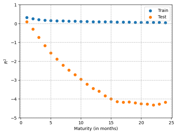
First, it is remarkable that the cut-off lags $C_{R_{1}}$ all are below 100 days except for the largest maturities. Second, the cut-off lags $C_{\Sigma}$ are above 1,000 days for all maturities except the first one for the S&P 500 and the first two for the Euro Stoxx 50. Looking at the average $R^{2}$ scores for all tested triplets, we observed that the fitting quality is very sensitive to the cut-off lag $C_{\Sigma}$ of the volatility feature while the two other hyperparameters $C_{R_{1}}$ and $\lambda$ have a smaller influence (especially $\lambda$ which can explain the wide range of values obtained for this hyperparameter in Table 1). Choosing a too small cut-off lag $C_{\Sigma}$ can lead to very low $R^{2}$ scores, especially for the largest maturities. For example, for $C_{\Sigma}=500$ , we obtain $R^{2}$ scores that are even below 0 for the Euro Stoxx 50, as illustrated in Figure 6. Actually any value $C_{\Sigma}$ strictly below 1000 in the grid $\{5,10,25,50,100,250,500,1000,1500,2000,2500,3000\}$ yields overall poor results such as those exhibited in Figure 6 and this regardless of the value of $C_{R_{1}}$ . This indicates that the squared returns up to 1,000 business days in the past are paramount to predict the implied volatility, particularly for the largest maturities.

In order to verify that this conclusion is not an artefact of a bad model calibration, we present in Figure 7 the correlation between the implied variance and the squared daily returns for all lags between 0 and 3,000 days both on the train and the test sets. Note that the estimated correlation $\rho$ is presented along with a 95% confidence interval derived from the transformation $z=\text{artanh}(\rho)$ introduced by Fisher (1915). Indeed, this transformation is approximately normally distributed when the samples come from a bivariate normal distribution. Although this is not the case here, we consider it as a reasonable proxy of the uncertainty around the correlation estimator. On the train set (blue curve), the graphs show a slow decrease of the correlation with the lag, with several spikes at some specific lags that become larger when the maturity increases. A first spike can be seen around 250 days, i.e. 1 year, especially for the Euro Stoxx 50. Then a smaller spike can be seen around 500 days, i.e. 2 years. A third spike appears around 750 days, i.e. 3 years, which is characterized by a slower decay than the previous spikes as it only fades around 1,250 days. This third spike is even higher than the previous spikes for large maturities. After these three spikes, we observe again smaller spikes around 1,750 days and 2,500 days and again a big spike around 2,750 days, that is a spike almost every year. These observations are consistent with the sensitivity of the model to the cut-off lag $C_{\Sigma}$ and the values obtained with the cross-validation that are presented in Table 1. Note that these observations have the advantage of not depending on any assumption. Thus, we can consider the long-range dependence of the implied volatility to the past squared returns as a stylized fact of our implied volatility data. An empirical study of a larger set of underlying assets could reveal whether this is a universal property of implied volatility data. To our knowledge, this stylized fact has never been reported in the literature. Let us however mention the work of Härdle and Mungo (2007) who calibrate a 3-factors model on implied volatility data and show a long-range dependence in the level and absolute returns of the factors loading series. A possible explanation of this phenomenon is that options on widespread equity indices and with relatively large maturities are presumably traded by long-term investors such as asset managers, pension funds, sovereign funds, etc. who have a low rebalancing frequency of their portfolios and consequently, who base their investment decisions on the previous years returns of the underlying asset rather than the previous days returns. On the other hand, options with shorter maturities are presumably less traded by long-term investors so that the movements of the implied volatility are more influenced by short-term investors such as hedge funds who base their investment decisions on recent data. This is in line with Figures 7(a) and 7(d) as well as with the smaller values of $C_{\Sigma}$ for the smallest maturities in Table 1. In Figure 8, we also present the correlations between the implied volatility and the daily returns for all lags between 0 and 3,000 days both on the train and the test sets. In this case, the correlations fades very quickly with the lag and we do not observe material spikes. This is consistent with the smaller values of $C_{R_{1}}$ in Table 1.

So far, we have only described the correlations on the train set but as already discussed extensively, the test set is quite different and the correlations on this set (in orange in Figures 7 and 8) are therefore also distinct from those calculated on the train set. In particular in Figure 7, we observe negative correlations with the 250 days lag which can be understood as a consequence of the fact that the implied volatility was decreasing in 2021 due to the leverage effect while one year earlier the squared returns were increasing with the Covid-19 crisis. Conversely, the implied volatility increased in 2022 again due to the leverage effect while one year earlier the squared returns were decreasing with the post-Covid-19 bull market. Given the particular profile of the correlation structure, it is natural to consider a variation of the PDV model that allows to capture the spikes. We have considered two variations of the PDV model allowing to capture the spike at the 3-years lag as it represents the larger spike. These two variations consist in adding a third feature which is the same as the volatility feature $\Sigma$ except that the kernel weights specifically one period in the past. The two kernels that we have considered are the following:

K_{2}^{\prime}(\tau)=(a\tau-\delta)^{+}\exp(-\lambda\tau)\text{ and }K_{2}^{\prime\prime}(\tau)=\exp\left(-\frac{(\tau-\mu)^{2}}{\sigma^{2}}\right)

(2.5)

where $a$ , $\delta$ , $\lambda$ , $\mu$ and $\sigma$ are non-negative parameters. The calibration of these alternative models only provides a small improvement of the $R^{2}$ scores on the train set and even a deterioration of the $R^{2}$ scores on the test set, likely due to the specificity of the test set mentioned earlier. As a consequence, these alternative models are disregarded in the sequel.

2.3.5 Study of the calibrated parameters

We conclude this empirical study by analyzing the calibrated parameters of the PDV model. In order to obtain comparable model parameters between maturities, we retain a single triplet $(C_{R_{1}},C_{\Sigma},\lambda)$ for all maturities. This triplet is selected as follows. For each maturity, we compute the average $R^{2}$ score over the 10 folds of each triplet and then, we average these scores over all maturities. Finally, for each triplet $(C_{R_{1}},C_{\Sigma},\lambda)$ , we average the obtained score with the one of the triplets $(C_{R_{1}}^{\prime},C_{\Sigma}^{\prime},\lambda^{\prime})$ such that $C^{\prime}_{\Sigma}=C_{\Sigma}$ and either $C_{R_{1}}^{\prime}$ is the closest value above or below $C_{R_{1}}$ in the grid $\{5,10,25,50,100,250,500,1000,\dots,2500,3000\}$ or $\lambda^{\prime}$ is the closest value above or below $\lambda$ in the grid $\{10^{-6},10^{-5},\dots,10^{-1}\}$ . For example, the score of the triplet $(50,500,10^{-3})$ is averaged with the one of the triplets $(25,500,10^{-3})$ , $(100,500,10^{-3})$ , $(50,500,10^{-4})$ and $(50,500,10^{-2})$ . The triplet that is chosen for all maturities is the one achieving the higher score through this procedure. This procedure aims at selecting a triplet whose performance is not too sensitive to a modification of $C_{R_{1}}$ or $\lambda$ and is introduced because we observed that if we consider only the average score over all maturities, the performance of the obtained triplet was very sensible to these two hyperparameters (unlike most triplets as underlined earlier) and was quite bad on the test set. This instability is probably due to the small size of the train set which is divided in 10 folds in the blocked cross-validation. With this procedure, we obtain $(C_{R_{1}},C_{\Sigma},\lambda)=(100,1000,10^{-4})$ for the S&P 500 and $(C_{R_{1}},C_{\Sigma},\lambda)=(10,1000,10^{-3})$ for the Euro Stoxx 50. In Figure 9, we show the $R^{2}$ scores obtained on the train and the test sets with these hyperparameters. We notice overall a small deterioration in comparison with Figure 3 where $(C_{R_{1}},C_{\Sigma},\lambda)=(1000,1000,0)$ . This deterioration can be attributed to the fact that the hyperparameters are optimized on the train set only which differs in several ways from the test set.

In Figures 10 and 11, we plot the evolution of the calibrated parameters associated to the $R^{2}$ scores presented in Figure 9 as a function of the maturity. Regarding the TSPL kernels parameters ( $\alpha_{1}$ , $\delta_{1}$ , $\alpha_{2}$ , $\delta_{2}$ ), we observe overall a decreasing trend except for $\delta_{2}$ for which there is no clear trend. This decreasing trend for $\alpha_{1}$ and $\alpha_{2}$ indicates that far away past returns explain more and more the ATM implied volatility movements as the maturity increases. Note that, for the largest maturities, we obtain values of $\alpha$ that become even lower than 1 (except for $\alpha_{1}$ for the S&P 500) which is the critical value below which the integral of the TSPL kernel diverges in continuous time. The decreasing behavior of $\delta_{1}$ indicates that, as $\alpha_{1}$ decreases, it still matters to keep a large weight for the more recent returns. Let us now end the study with the analysis of the parameters $\beta_{0}$ , $\beta_{1}$ and $\beta_{2}$ . First, we notice that we have $\beta_{1}<0$ and $\beta_{2}>0$ without imposing any constraint on these parameters. Therefore, a positive (resp. negative) trend in the underlying asset price tends to be followed by a decrease (resp. increase) of the implied volatility (which is consistent with the negative correlation observed by Cont and da Fonseca (2002)) while the increase (resp. decrease) of the underlying asset volatility (measured by the squared

returns) tends to be followed by an increase (resp. decrease) of the implied volatility. Moreover, the three parameters for the small maturities are of the same order of magnitude as to those calibrated by Guyon and Lekeufack (2023). Regarding the evolution of $\beta_{0}$ , we obtain an overall increase with the maturity which reflects the fact that, in average, the level of ATM implied volatility increases with the maturity. The parameter $\beta_{1}$ , which can be interpreted as the influence of the trend feature on the implied volatility, is getting closer to 0 with the maturity, implying that the implied volatility for long maturities becomes less reactive to the trend in the returns of the underlying asset price. Finally, the parameter $\beta_{2}$ , which can be interpreted as the influence of the volatility feature on the implied volatility, is mainly decreasing with the maturity, so it seems that the implied volatility for long maturities becomes less reactive to the volatility of the underlying index.

The empirical study conducted in this section allowed us to exhibit the dependence of the ATM implied volatility on the past path of the underlying asset price for two major financial indices. We showed that this dependence decreases with the maturity but remains material even for the largest maturities. Moreover, the feedback effect of the underlying price onto the ATM implied volatility has a very long memory: up to 4 years of the past evolution of the underlying price should be used to predict the ATM implied volatility for the largest maturities. At this stage, it is natural to ask whether these conclusions still hold for away-from-the-money implied volatilities. Instead of reproducing the empirical study for each maturity and strike (which would increase significantly the dimension of the study), we study the performance of the PDV model in explaining the evolution of the calibrated parameters of the SSVI parameterization of Gatheral and Jacquier (2014). The following section is dedicated to the presentation of this parameterization.

3 Calibration of market implied volatilities with the SSVI parameterization

The purpose of this section is to introduce the SSVI parameterization and to present some calibration results of this model on the implied volatility historical data that we considered in Section 2. We start by some remainders about static arbitrages as the ability to generate arbitrage-free implied volatility surfaces (IVSs) is one of our motivations for considering the SSVI parameterization.

3.1 Static arbitrages

An IVS is free from static arbitrage if there is no arbitrage opportunity by static trading of call and put options with prices given by inserting their implied volatility in the Black-Scholes formula. The formal definition of absence of static arbitrage is provided below.

Definition 3.1 (Absence of static arbitrage).

Let us denote $C_{BS}(K,T,\sigma)$ the Black-Scholes price of an European call option of strike $K$ and maturity $T$ when the constant volatility is $\sigma$ . An IVS $(K,T)\mapsto\sigma_{BS}(K,T)$ is free of static arbitrage if there exists a non-negative martingale, say $(S_{t})_{t\geq 0}$ , on some filtered probability space $(\Omega,\mathcal{F},\mathbb{P})$ such that $C(K,T):=C_{BS}(K,T,\sigma_{BS}(K,T))=\mathbb{E}[e^{-rT}(S_{T}-K)^{+}]$ for all $K,T\geq 0$ and where $r$ is the risk-free interest rate.

Roper (2010) provides sufficient conditions under which an IVS is free of static arbitrage.

Theorem 3.1 (Theorem 2.9. from Roper, 2010).

Consider the total implied variance defined by $w(k,T)=\sigma_{BS}^{2}(k,T)T$ where $\sigma_{BS}(k,T)$ is the Black-Scholes implied volatility associated to the log-strike³³3We recall that the log-strike $k$ of a vanilla option of strike $K$ and forward price $F=S_{0}e^{rT}$ is defined as $k=\log\left(\frac{K}{F}\right)$ $k$ and the maturity $T$ . If $w:\mathbb{R}\times\mathbb{R}_{+}\rightarrow\mathbb{R}_{+}$ satisfies the following conditions:

(i)

$w(\cdot,T)$ is of class $C^{2}$ for all $T\geq 0$ ,
(ii)

$w(k,T)>0$ for all $(k,T)\in\mathbb{R}\times\mathbb{R}_{+}^{*}$ ,

(iii)

for each $(k,T)\in\mathbb{R}\times\mathbb{R}_{+}^{*}$ ,

\left(1-\frac{k\partial_{k}w(k,T)}{2w(k,T)}\right)^{2}-\frac{\partial_{k}w(k,T)^{2}}{4}\left(\frac{1}{w(k,T)}+\frac{1}{4}\right)+\frac{\partial^{2}_{kk}w(k,T)}{2}\geq 0,

(3.1)

(iv)

$w(k,\cdot)$ is non-decreasing for each $k\in\mathbb{R}$ ,
(v)

$-k/\sqrt{w(k,T)}+\sqrt{w(k,T)}/2\underset{k\to+\infty}{\rightarrow}-\infty$ for all $T>0$ and,
(vi)

$w(k,0)=0$ for all $k\in\mathbb{R}$ ,

then the total implied variance surface $w$ is free of static arbitrage.

Remark 3.1.

An IVS is said to be free of butterfly arbitrage if conditions $(iii)$ and $(v)$ are satisfied and it is said to be free of calendar spread arbitrage if condition $(iv)$ is satisfied. To our knowledge, this terminology is due to Gatheral and Jacquier (2014).

3.2 The SSVI parameterization

Devised at Merill Lynch in 1999 and publicly disseminated by Gatheral (2004), the Stochastic Volatility Inspired (SVI) parameterization is a popular parameterization of the implied volatility smile. To be more precise, it is a parameterization of the total implied variance that we defined in Theorem 3.1. The standard formulation of the SVI parameterization is the so-called raw SVI parameterization and is presented below.

Definition 3.2 (Raw SVI).

For a given maturity $T>0$ , the raw SVI parameterization writes:

w(k,T)=a_{T}+b_{T}\left(\rho_{T}(k-m_{T})+\sqrt{(k-m_{T})^{2}+\sigma_{T}^{2}}\right)

(3.2)

where $a_{T}\in\mathbb{R}$ , $b_{T}\geq 0$ , $|\rho_{T}|<1$ , $m_{T}\in\mathbb{R}$ and $\sigma_{T}>0$ . Moreover, the parameters must satisfy $a_{T}+b_{T}\sigma_{T}\sqrt{1-\rho^{2}_{T}}\geq 0$ to ensure that the total implied variance remains positive for all $k\in\mathbb{R}$ .

The popularity of this parameterization is mainly due to its tractability and its ability to fit market implied volatilities quite well. Moreover, it features nice properties such as consistency with Lee’s moment formula (Lee, 2004) or the fact that it corresponds exactly to the large-maturity limit of the Heston implied volatility smile (Gatheral and Jacquier, 2011). In their paper, Gatheral and Jacquier (2014) proposed an extension of the SVI parameterization to address two issues of this parameterization. First, the SVI parameterization is not a parameterization of the full total implied variance surface but only of a slice $k\mapsto w(k,T)$ for a fixed maturity $T$ since the 5 parameters are all maturity-dependent. Second, at the time of the publication of their paper, it seemed impossible to find conditions on the SVI parameters that guarantee the absence of butterfly arbitrage (the problem has now been solved by Martini and Mingone, 2022). The extension of the SVI parameterization that they propose to address these issues is called the surface SVI (SSVI) and is defined below.

Definition 3.3.

Let $\varphi$ be a smooth function from $\mathbb{R}_{+}^{*}$ to $\mathbb{R}_{+}^{*}$ such that the limit $\lim_{T\to 0}\theta_{T}\varphi(\theta_{T})$ exists in $\mathbb{R}$ where $\theta_{T}:=\sigma_{BS}^{2}(0,T)T$ is the ATM total implied variance. The SSVI is the surface defined by:

w(k,T)=\frac{\theta_{T}}{2}\left(1+\rho\varphi(\theta_{T})k+\sqrt{(\varphi(\theta_{T})k+\rho)^{2}+(1-\rho^{2})}\right).

(3.3)

Remark 3.2.

By abuse of notation, we use the same notation $\sigma_{BS}$ for the implied volatility as a function of the strike or the implied volatily as a function of the log-strike.

While the SVI parameterization requires 5 parameters for each slice of the IVS, the SSVI relies on the function $\varphi$ and the parameter $\rho\in(-1,1)$ , that do not depend on the maturity, as well as one parameter $\theta_{T}$ for each maturity that depends on the maturity but could be considered as set prior to the calibration since the ATM total implied variance for the traded maturities can be directly observed on the market. Note that Hendriks and Martini (2017) propose to consider a maturity-dependent $\rho$ parameter in order to improve the calibration accuracy for very short maturities (typically below 1 month). Since our database does not contain short-term data, this extension of the SSVI is not investigated in this paper.

Remark 3.3.

For a fixed $T>0$ , the corresponding raw SVI parameterization is given by $(a_{T},b_{T},\rho_{T},m_{T},\sigma_{T})=\left(\frac{\theta_{T}}{2}(1-\rho^{2}),\frac{\theta_{T}\varphi(\theta_{T})}{2},\rho,-\frac{\rho}{\varphi(\theta_{T})},\frac{\sqrt{1-\rho^{2}}}{\varphi(\theta_{T})}\right)$ .

Gatheral and Jacquier provide sufficient conditions for the SSVI to be free of arbitrage. These conditions are presented in the following theorem.

Theorem 3.2 (Corollary 4.1 from Gatheral and Jacquier (2014)).

The SSVI is free of static arbitrage if the following conditions are satisfied:

(i)

$\partial_{T}\theta_{T}\geq 0$ for all $T>0$ ;
(ii)

$0\leq\partial_{\theta}(\theta\varphi(\theta))\leq\frac{1}{\rho^{2}}\left(1+\sqrt{1-\rho^{2}}\right)\varphi(\theta)$ for all $\theta>0$ ;
(iii)

$\theta\varphi(\theta)(1+|\rho|)<4$ for all $\theta>0$ ;
(iv)

$\theta\varphi(\theta)^{2}(1+|\rho|)\leq 4$ for all $\theta>0$ .

Remark 3.4.

The conditions (i) and (ii) actually are necessary and sufficient conditions for the absence of calendar spread arbitrage for the SSVI. The condition (iii) with a non-strict inequality is a necessary condition for the absence of butterfly arbitrage but condition (iv) is only a necessary condition if $\theta\varphi(\theta)(1+|\rho|)=4$ .

Remark 3.5.

The conditions (ii), (iii) and (iv) can be weakened as follows:

(ii)

$0\leq\partial_{\theta}(\theta\varphi(\theta))\rvert_{\theta=\theta_{T}}\leq\frac{1}{\rho^{2}}\left(1+\sqrt{1-\rho^{2}}\right)\varphi(\theta_{T})$ for all $T>0$ ;
(iii)

$\theta_{T}\varphi(\theta_{T})(1+|\rho|)<4$ for all $T>0$ ;
(iv)

$\theta_{T}\varphi(\theta_{T})^{2}(1+|\rho|)\leq 4$ for all $T>0$ .

Note that these conditions are not necessarily equivalent to the ones in Theorem 3.2 since $T\mapsto\theta_{T}$ is not necessarily a bijection from $\mathbb{R}_{+}^{*}$ to $\mathbb{R}_{+}^{*}$ .

A natural question at this stage is how to choose the function $\varphi$ in order to both achieve a good fit to market data and satisfy the above conditions. The authors propose three examples of parametric form for $\varphi$ :

•

the Heston-like parameterization $\varphi(\theta):=\frac{1}{\lambda\theta}\left(1-\frac{1-e^{-\lambda\theta}}{\lambda\theta}\right)$ with $\lambda>0$ ,
•

the power-law parameterization $\varphi(\theta):=\frac{\eta}{\theta^{\gamma}}$ with $\eta>0$ and $0<\gamma<1$ , and
•

the modified power-law parameterization $\varphi(\theta):=\frac{\eta}{\theta^{\gamma}(1+\theta)^{1-\gamma}}$ with $\eta>0$ and $0<\gamma<1$ .

For simplicity of reference to these parameterizations, we abbreviate the SSVI with the Heston-like parameterization to SSVI-HL, the SSVI with the power-law parameterization to SSVI-PL and the SSVI with the modified power-law parameterization to SSVI-MPL. The following propositions translate the sufficient conditions of Theorem 3.2 for these three parameterizations. Their proof can be found in Appendix A.

Proposition 3.1.

The SSVI-HL is free of static arbitrage if $\partial_{T}\theta_{T}\geq 0$ for all $T>0$ and $\lambda\geq(1+|\rho|)/4$ .

Proposition 3.2.

Assuming that $\partial_{T}\theta_{T}\geq 0$ , we have the following cases:

(i)

If $\gamma\in(0,1/2)$ , there exists $\theta_{1}^{*},\theta_{2}^{*}>0$ such that the SSVI-PL is free of static arbitrage if $\theta_{T}<\theta_{1}^{*}\wedge\theta_{2}^{*}$ for all $T>0$ .
(ii)

If $\gamma\in(1/2,1)$ , there exists $\theta_{1}^{*},\theta_{2}^{*}>0$ such that the SSVI-PL is free of static arbitrage if $\theta_{2}^{*}<\theta_{T}<\theta_{1}^{*}$ for all $T>0$ .
(iii)

If $\gamma=1/2$ and $\eta^{2}(1+|\rho|)\leq 4$ , there exists $\theta_{1}^{*}$ such that the SSVI-PL is free of static arbitrage if $\theta_{T}<\theta_{1}^{*}$ for all $T>0$ .

Proposition 3.3.

Assuming that $\partial_{T}\theta_{T}\geq 0$ , we have the following cases:

(i)

If $\gamma\in(0,1/2)$ and $\eta(1+|\rho|)\leq 4$ , there exists $\theta^{*}>0$ such that the SSVI-MPL is free of static arbitrage if, for all $T>0$ , $\theta_{T}\geq\theta^{*}$ .
(ii)

If $\gamma\in(1/2,1)$ , the SSVI-MPL is free of static arbitrage for $\eta(1+|\rho|)\leq 4$ and $(1-2\gamma)\varphi(1-2\gamma)^{2}(1+|\rho|)\leq 4$ .
(iii)

If $\gamma=1/2$ , the SSVI-MPL is free of static arbitrage for $\eta^{2}(1+|\rho|)\leq 4$ .

Remark 3.6.

Note that different sufficient conditions could be found for guaranteeing the absence of static arbitrage by restricting the maturity $T$ to some subset of $\mathbb{R}_{+}^{*}$ . Since it is not very satisfying to have an IVS parameterization that could be arbitrable for some maturities, we looked as much as possible for conditions that do not restrict the values of $T$ .

Remark 3.7.

For $\gamma=1/2$ , the SSVI-PL and the SSVI-MPL parameterizations induce a power-law decay of the ATM volatility skew for small maturities which is a well-known stylized fact of implied volatility surfaces (see e.g. Gatheral et al., 2023). Indeed, recalling that the ATM volatility skew is defined by $\partial_{k}\sigma_{BS}(0,T)$ , it is straightforward to show that $\partial_{k}\sigma_{BS}(0,T)=\frac{1}{2\sqrt{T}}\rho\sqrt{\theta_{T}}\varphi(\theta_{T})$ for the SSVI parameterization (no matter the choice for $\varphi$ ). Therefore, we have that $\partial_{k}\sigma_{BS}(0,T)=\frac{\rho\eta}{2\sqrt{T}}$ for the SSVI-PL and $\partial_{k}\sigma_{BS}(0,T)=\frac{\rho\eta}{2\sqrt{T}\sqrt{1+\theta_{T}}}=\frac{\rho\eta}{2\sqrt{T}}+o\left(\frac{1}{\sqrt{T}}\right)$ for the SSVI-MPL assuming that $\lim_{T\to 0}\theta_{T}=0$ which is a natural assumption: an ATM option with zero time to expiry has no value.

3.3 Calibration results and introduction of the parsimonious SSVI model

In this section, we show to which extent the SSVI parameterization allows to replicate the historical IVSs that we presented in Section 2.1. As already noted by Cont and Vuletić (2023), IVSs from data providers are not necessarily arbitrage-free because of interpolations of actual market quotes. Procedures such as the ones of Davis and Hobson (2007) or Cohen et al. (2020) allow to detect arbitrages in a finite set of prices of European call options given the forward prices. Our database does not contain short rates data or forward prices data so we cannot use these procedures. Since calendar spread arbitrages are equivalent to the total implied variance being non-decreasing in maturity, we remove the IVSs (we recall that our data sets contain one IVS per business day) such that there is at least one crossing between the linearly interpolated total implied variances of two adjacent maturities. IVSs with butterfly arbitrages (if any) are not removed as the condition in terms of total implied variance is much more complicated to verify (see condition (iii) of Theorem 3.1). In total, 6.4% (resp. 5.6%) of the IVSs are removed from the S&P 500 (resp. Euro Stoxx 50) data set.

We start by comparing the three parametric forms of the function $\varphi$ that we introduced in the previous section. For this purpose, we calibrate the SSVI for each day of our data sets without calendar spread arbitrages and for each parametric form of $\varphi$ by solving the following minimization problem using the minimize function with the SLSQP algorithm from the scipy Python package:

\begin{array}[]{rrrcllr}\displaystyle\min_{\Theta=((\theta_{T_{i}})_{i=1,\dots,M},\rho,\Pi_{\varphi})}&\lx@intercol\hfil\displaystyle\sum_{i=1}^{M}\sum_{k\in\mathcal{K}_{T_{i}}}\phi(k)\left(\sigma_{Mkt}(k,T_{i})-\sigma_{SSVI}(k,T_{i};\Theta)\right)^{2}\hfil\lx@intercol\\ \text{s.t.}&\theta_{T_{1}}&\geq&0&&\\ &\theta_{T_{i+1}}&\geq&\theta_{T_{i}}&\text{for }1\leq i\leq M-1&\\ &(\rho,\Pi_{\varphi})&\in&C_{\varphi}.&&\end{array}

(3.4)

We used the following notations:

•

$\Pi_{\varphi}$ is the vector of the parameters in $\varphi$ : only $\lambda$ for the SSVI-HL and $(\eta,\gamma)$ for the SSVI-PL and the SSVI-MPL.
•

$T_{1}<T_{2}<\dots<T_{M}$ is the set of maturities and $\mathcal{K}_{T}$ is the set of log-strikes for the maturity $T$ .
•

$\phi(k)$ is the standard normal density function evaluated in the log-strike $k$ . This weighting function allows to give more weight to the replication of the implied volatilities that are close to the money. Another choice based on the Black-Scholes vega has been considered but we did not notice any improvement.
•

$\sigma_{Mkt}$ is the market implied volatility.
•

$\sigma_{SSVI}(\cdot,\cdot;\Theta)$ is the SSVI implied volatility associated to the parameter vector $\Theta=((\theta_{T_{i}})_{i=1,\dots,M},\rho,\Pi_{\varphi})$ .

•

$C_{\varphi}$ is given by:

–

$C_{\varphi}=\{(\rho,\lambda)\in(-1,1)\times\mathbb{R}_{+}^{*}\mid\lambda\geq(1+|\rho|)/4\}$ for the SSVI-HL,
–

$C_{\varphi}=\{(\rho,\eta,\gamma)\in(-1,1)\times\mathbb{R}_{+}^{*}\times(0,1)\mid\eta^{2}(1+|\rho|)\leq 4\text{ if }\gamma=1/2\}$ for the SSVI-PL and,

–

C_{\varphi}=\left\{(\rho,\eta,\gamma)\in(-1,1)\times\mathbb{R}_{+}^{*}\times(0,1)\left|\begin{array}[]{ll}\eta(1+|\rho|)\leq 4&\text{ if }\gamma<1/2\\ \eta(1+|\rho|)\leq 4\text{ and }(1-2\gamma)\varphi(1-2\gamma)^{2}(1+|\rho|)\leq 4&\text{ if }\gamma>1/2\\ \eta^{2}(1+|\rho|)\leq 4&\text{ if }\gamma=1/2\end{array}\right.\right\}

for the SSVI-MPL.

Remark 3.8.

The constraints in the above minimization problem do not guarantee the absence of static arbitrage for the power-law and the modified power-law parameterizations as far as only the constraints involving $\rho$ , $\eta$ and $\gamma$ are included as well as the non-decreasing property of $T\mapsto\theta_{T}$ . The reason for this choice is the fact that there is no closed-form expression for $\theta^{*}$ , $\theta_{1}^{*}$ and $\theta_{2}^{*}$ so the addition of the constraints involving these terms would strongly complexify the numerical optimization. By the end of this section, the study will be restricted to the SSVI-MPL parameterization with $\gamma=1/2$ (for which there is no constraint involving $\theta^{*}$ , $\theta_{1}^{*}$ or $\theta_{2}^{*}$ ) so this choice is impact-free.

Remark 3.9.

We use in practice the change of variable $(\tilde{\theta}_{T})_{i=1,\dots,M}$ where $\tilde{\theta}_{T_{1}}=\theta_{T_{1}}$ and $\tilde{\theta}_{T_{i}}=\theta_{T_{i}}-\theta_{T_{i-1}}$ for $i\in\{2,\dots,M\}$ since it allows to transform the second inequality constraints in the minimization problem (3.4) in bounds constraints: $\tilde{\theta}_{T_{i}}\geq 0$ for $2\leq i\leq M$ .

The initial guess for each parameter is provided in Table 2. The average relative errors (without weighting) between the market implied volatilities and the SSVI implied volatilities for each day of our data sets are presented in Figure 12. It appears clearly that the Heston-like parameterization performs very poorly in comparison to the two others parameterizations. This results from the fact that, in the Heston-like parameterization, the function $\varphi$ is bounded from above by $1/2$ (see Appendix A.1) which constraints strongly the shape of the IVS. The power-law and the modified power-law parameterizations achieve essentially the same accuracy which is very stable over time. In particular, we do not observe a decrease of the fitting quality during the Covid-19 crisis. In Figure 13, we illustrate how the SSVI-MPL fits the S&P 500 (resp. the Euro Stoxx 50) total implied variances for a day where the calibrated average relative error is equal to 1.19% (resp. 1.18%) corresponding to the mean of the average relative errors across the whole S&P 500 (resp. Euro Stoxx 50) data set.

Table 2: Initial guesses provided to the optimization routine.

$(\theta_{T_{i}})_{i=1,\dots,M}$	$\rho$	$\lambda$	$\eta$	$\gamma$
$(\sigma_{Mkt}(0,T_{i})^{2}T_{i})_{i=1,\dots,M}$	-0.5	1	1	0.25

At this stage, let us recall that our final objective is to design a model to jointly simulate arbitrage-free IVSs and the price of the underlying asset by simulating the evolution of the SSVI parameters as a function of the path of the underlying asset price. However, the number of parameters involved is so large that a model for their joint evolution would be too complicated. Therefore, we need to make the SSVI model more parsimonious. We propose the two following simplifications:

1.

We consider only the modified power-law parameterization with $\gamma$ fixed to 1/2 because we observe that $\gamma$ is close to this value over the two data sets (more than 84% of the calibrated $\gamma$ ’s lie within the $[0.4,0.6]$ interval). Moreover, this choice has the advantage of guaranteeing that the full surface (without any restriction on the ATM total implied variance) is free of static arbitrage on the sole condition that $\eta^{2}(1+|\rho|)<4$ . Finally, according to Remark 3.7, setting $\gamma=1/2$ implies a power-law decay of the ATM volatility skew which is a known stylized fact.
2.

We assume that $\theta_{T}=aT^{p}$ where $a,p\geq 0$ reducing considerably the number of parameters while ensuring that the no-arbitrage constraint on the ATM total variance is always satisfied ( $\partial_{T}\theta_{T}\geq 0$ ). This parametric form is inspired by the calibrated vectors $(\theta_{T_{i}})_{i=1,\dots,M}$ that exhibit almost a linear behavior with the maturity $T$ . In Figure 14, we show how this parametric form fits the S&P 500 ATM total variances for several dates (the fit is similar for the Euro Stoxx 50 so it is not shown here). Note that the parameters $a$ and $p$ that have been used in this figure are those calibrated on the whole IVS so the quality of the fit is reduced in comparison to a calibration on the ATM volatilities only. Despite this, the fit is overall satisfying although the concave shapes of the ATM total variances in Figure 14(b) cannot be well reproduced.

The new model obtained after these simplifications is called thereafter the parsimonious SSVI model.

Definition 3.4 (Parsimonious SSVI).

The parsimonious SSVI is the parameterization of the total implied volatility surface defined by:

w(k,T)=\frac{\theta_{T}}{2}\left(1+\rho\varphi(\theta_{T})k+\sqrt{(\varphi(\theta_{T})k+\rho)^{2}+(1-\rho^{2})}\right).

(3.5)

where $\theta_{T}=aT^{p}$ and $\varphi(\theta)=\frac{\eta}{\sqrt{\theta(1+\theta)}}$ with $a,p\geq 0$ and $\eta>0$ .

In Figure 15, the average relative errors between the market implied volatilities and the SSVI implied volatilities for each day of our data sets obtained for the parsimonious SSVI model are compared to those obtained for the SSVI model with the modified power-law parameterization.

As expected, the calibration accuracy is reduced for the parsimonious SSVI. However, it remains overall quite close to the SSVI-MPL calibration in view of the reduction of the number of parameters: 4 parameters for the parsimonious SSVI versus 27 for the SSVI-MPL. The mean of the average relative errors across the whole S&P 500 (resp. Euro Stoxx 50) data set increases from 1.19% (resp. 1.18%) to 1.65% (resp. 1.60%). In Figure 16, we show the impact of each simplification on the calibration accuracy for the S&P 500 (it is similar for the Euro Stoxx 50). It appears very clearly that the parametric form for $\theta_{t}$ is the assumption leading to the largest deterioration of the fit to market implied volatilities, which is consistent with the fact that this assumption is the one limiting the most the number of degrees of freedom of the model.

4 Path-dependent SSVI model

The present section is dedicated to the introduction of a new model for the joint dynamics of an implied volatility surface and the underlying asset price. The calibration results exposed in Section 3.2 demonstrate the ability of a particular case of the SSVI parameterization - the parsimonious SSVI - to fit reasonably well historical implied volatility surfaces while guaranteeing the absence of static arbitrage with only 4 parameters. As a consequence, we propose to specify our model as a dynamic version of the parsimonious SSVI: each parameter of the parsimonious SSVI is considered as a stochastic process whose dynamics remains to be determined. One option to jointly model the evolution of the parsimonious SSVI parameters and the underlying asset would be to introduce a correlation between the random noises driving each process. However, in view of the empirical study conducted in Section 2 which indicates that there is a feedback effect of the past returns and the past squared returns of the underlying index price onto the level of the ATM implied volatility, we prefer another option. Instead of using a correlation, the idea is to explicitly model the response of each of the 4 parameters to the evolution of the underlying asset price. To this end, we measure to which extent the trend feature and the volatility feature of the path-dependent volatility (PDV) model presented in Section 1.2 allow to explain the variations of the 4 parameters of the parsimonious SSVI model. This study is presented in Section 4.1 below. Then, Section 4.2 introduces a variant of the PDV model of Guyon and Lekeufack and the dynamics of the parsimonious SSVI parameters. Finally, Section 4.3 and 4.4 detail the calibration and the simulation of the model.

4.1 Path-dependency of the parsimonious SSVI parameters

The calibration of the parsimonious SSVI in Section 3.3 provides the daily evolutions of the parameters $a$ , $p$ , $\rho$ and $\eta$ . Based on these daily evolutions, we can calibrate the PDV model (1.1) where we replace $Volatility_{t}$ in Equation (1.1) by each parameter of the parsimonious SSVI. Note that we consider the logarithm of $p$ instead of $p$ in the PDV model since we observed that this provides a better fit. The calibration methodology is the same as the one exposed in Section 2.2. Moreover, similarly to the study in Section 2.3, for each parameter of the parsimonious SSVI, we run a 10-fold blocked cross-validation on the train set to determine the optimal hyperparameters $C_{R_{1}}$ , $C_{\Sigma}$ and $\lambda$ in the grid $\{5,10,25,50,100,250,500,1000,1500,2000,2500\}^{2}\times\{10^{-6},10^{-5},\dots,10^{-1}\}$ . The $R^{2}$ scores obtained on the train and the test sets for each parameter and for each index are reported in Table 3. On the one hand, these results show that the time evolution of the parameter $a$ is well explained by the evolution of the underlying asset price both on the train and the test sets, which is line with the results obtained for the ATM implied volatility since $a$ captures the ATM total variance level (whose evolution is similar to the one of the ATM implied volatility and as such we expect the study conducted in Section 2.3 to be still valid for the ATM total variance). The same observation holds for $p$ . However the fact that the PDV model works well for $p$ was not anticipated as it allows to parameterize how the ATM total variance increases with the maturity and it is not homogenous to the ATM total variance level. Thus, we emphasize that this is a key finding. On the other hand, the $R^{2}$ scores for the parameters $\rho$ and $\eta$ are small on the train set and negative on the test set (except for $\rho$ on the Euro Stoxx 50). This indicates that the trend and the volatility features are not related to these two parameters. These observations come as no suprise: $\rho$ and $\eta$ parameterize respectively the orientation and the convexity of the implied volatility smile as illustrated in Figure 17. It is therefore less clear how the past variations of the underlying asset price could impact these parameters.

Remark 4.1.

Guyon and Lekeufack (2023) and Gazzani and Guyon (2023) considered a third feature given by $R_{1}^{2}\mathbb{1}_{\{R_{1}\geq 0\}}$ in the PDV model in order to achieve a satisfying joint SPX/VIX fit. Adding this feature to explain the variations of our 4 parameters does not improve the $R^{2}$ scores.

Table 3:

R^{2}

scores of the PDV model on the parameters of the parsimonious SSVI on the train and the test sets.

	S&P 500			Euro Stoxx 50
	$(C_{R_{1}},C_{\Sigma},\lambda)$	Train	Test	$(C_{R_{1}},C_{\Sigma},\lambda)$	Train	Test
$a$	(25,1000, $10^{-5}$ )	91.8%	51.1%	(10,1500, $10^{-3})$	85.7%	49.4%
$p$	(100,2000, $10^{-3}$ )	39.4%	48.5%	(250,50, $10^{-1}$ )	76.3%	75.3%
$\rho$	(100,5, $10^{-1}$ )	6.2%	-68.0%	(10,25, $10^{-3}$ )	35.9%	19.7%
$\eta$	(100,1500, $10^{-5}$ )	6.2%	-33.6%	(1000,1500, $10^{-3}$ )	58.0%	-899.5%

An idea to explain the variations of $\rho$ and $\eta$ is to consider skewness and kurtosis features. Indeed, Bouchaud and Potters (2003) showed a cumulant expansion formula for the Bachelier implied volatility allowing to explain the presence of the volatility smile and its shape using the skewness and the kurtosis of the underlying asset price distribution. Independently, Backus et al. (2004) showed a similar formula for the Black-Scholes implied volatility. This formula writes:

\sigma_{BS}(k,T)\simeq\sigma\left(1-\frac{\mu_{3}}{6}d-\frac{\mu_{4}}{24}(1-d^{2})\right)

(4.1)

where $\sigma$ , $\mu_{3}$ and $\mu_{4}$ are respectively the standard deviation, the skewness and the kurtosis of the log-return $\log\frac{S_{T}}{S_{0}}$ under the risk-neutral probability and $d=-k/\sigma+\sigma/2$ . Replacing $d$ by its expression in Equation (4.1) yields:

\sigma_{BS}(k,T)\simeq\sigma+\frac{k}{6}\mu_{3}-\frac{1}{12}\mu_{3}\sigma^{2}-\frac{1+k}{24}\mu_{4}\sigma+\frac{k^{2}}{24}\times\frac{\mu_{4}}{\sigma}+\frac{1}{96}\mu_{4}\sigma^{3}.

(4.2)

By analogy, we may consider the following regression model:

X_{t}=\beta_{0}+\beta_{1}\Sigma_{t}+\beta_{2}\mathcal{S}_{t}+\beta_{3}\mathcal{S}_{t}\Sigma_{t}^{2}+\beta_{4}\mathcal{K}_{t}\Sigma_{t}+\beta_{5}\frac{\mathcal{K}_{t}}{\Sigma_{t}}+\beta_{6}\mathcal{K}_{t}\Sigma_{t}^{3}

(4.3)

where $X_{t}$ is the value of either $\rho$ or $\eta$ at time $t$ , $\Sigma_{t}$ is the volatility feature (1.3) of the PDV model and $\mathcal{S}_{t}$ , $\mathcal{K}_{t}$ are respectively skewness and kurtosis features defined as:

	$\displaystyle\mathcal{S}_{t}$	$\displaystyle=\frac{\sum_{t_{i}\leq t}K_{3}(t-t_{i})r_{t_{i}}^{3}}{\Sigma_{t}^{3}},$		(4.4)
	$\displaystyle\mathcal{K}_{t}$	$\displaystyle=\frac{\sum_{t_{i}\leq t}K_{4}(t-t_{i})r_{t_{i}}^{4}}{\Sigma_{t}^{4}}.$		(4.4)

Note that the three kernels $K_{2}$ , $K_{3}$ and $K_{4}$ are assumed to be TSPL kernels. For the sake of simplicity, the cut-off lag is set to 1000 for all kernels and the penalization $\lambda$ is set to zero. The $R^{2}$ scores resulting from the calibration of this regression model are presented in Table 4. Note that we present both the scores obtained using the standard splitting of the data sets described in Section 2.1 and the average scores obtained using a 5-fold blocked cross-validation⁴⁴4We considered only 5 folds to limit the computational cost.. We remark that the scores are negative on the test set for all instances except for the parameter $\eta$ on the S&P 500 data set when using the standard splitting but it becomes negative with the 5-fold blocked cross-validation. To verify that these negative scores are not the consequence of an overfitted model, we tested the $2^{6}-1$ non-empty combinations of the 6 features in Equation (4.3) but we mostly obtained negative scores on the test set. For the instances where the score was positive on the test set, we ran a 5-fold blocked cross-validation which gave systematically negative scores on the test set. Therefore, we conclude that these 6 features are not relevant to predict the variations of the parameters $\rho$ and $\eta$ .

Table 4:

R^{2}

scores of the regression model (4.3) for

\rho

and

\eta

		S&P 500		Euro Stoxx 50
	5-fold blocked CV	Train	Test	Train	Test
$\rho$	No	43.6 %	-57554.5%	41.2%	-219.8%
$\rho$	Yes	46.6%	-22464.2%	44.1‘%	-104.3%
$\eta$	No	60.4%	75.7%	74.7%	-59.4%
$\eta$	Yes	64.4%	-3997.2%	83.5%	-169.5%

Beyond the interpretation of $\rho$ as a parameter that controls the orientation of the volatility smile, it is also possible to interpret it as the correlation between the two Brownian motions in the Heston model (the so-called "spot-vol" correlation) using the convergence of the Heston model towards the SVI parameterization (Gatheral and Jacquier, 2011). Because of this link, it is reasonable to study whether one can explain the variations of the parameter $\rho$ using the correlation between the underlying price and its volatility. As a measure of the volatility, we use the daily realized volatility estimates from Heber et al. (2009) spanning the period from January 1, 2000 to December 31, 2021. In the same spirit as the features of the PDV model, we introduce a correlation feature based on a TSPL kernel:

\Gamma_{t}=\frac{\sum_{t_{i}\leq t}K(t-t_{i})(r_{t_{i}}-\bar{r}_{t_{i}})(\sigma_{t_{i}}-\bar{\sigma}_{t_{i}})}{\sqrt{\sum_{t_{i}\leq t}K(t-t_{i})(r_{t_{i}}-\bar{r}_{t_{i}})^{2}\sum_{t_{i}\leq t}K(t-t_{i})(\sigma_{t_{i}}-\bar{\sigma}_{t_{i}})^{2}}}.

(4.5)

where $\bar{r}_{t_{i}}=\frac{1}{C+1}\sum_{k=0}^{C}r_{t_{i-k}}$ , $\sigma_{t}$ is the above-mentioned volatility and $\bar{\sigma}_{t_{i}}=\frac{1}{C+1}\sum_{k=0}^{C}\sigma_{t_{i-k}}$ . The calibration of the model $\rho_{t}=\beta_{0}+\beta_{1}\Gamma_{t}$ with a cut-off lag $C$ fixed to 1000 and a penalization $\lambda$ fixed to 0 again gives a very low $R^{2}$ score both on the train and test sets leading us to the conclusion that there does not seem to be any link in practice between the parameter $\rho$ in the SSVI and the correlation between the underlying price and its volatility.

4.2 Specification of the model for the underlying asset price and the IVS

Based on the analysis in the previous section, we provide in this section the dynamics of the four parameters in the parsimonious SSVI model. Since two of these parameters depend on the past path of the underlying asset price, we also need a model for the dynamics of the underlying asset price in order to be able to simulate IVSs over time. Because we want these simulations to be realistic, the model for the underlying asset price should also be as realistic as possible. We opt for the PDV model of Guyon and Lekeufack (more precisely, a variant of their model as we will see) as it allows to replicate almost all historical stylized facts of equity prices (leverage effect, volatility clustering, weak and strong Zumbach effects). The asset price $(S_{t})_{t\geq 0}$ is assumed to evolve as follows:

\left\{\begin{array}[]{rcl}\displaystyle\frac{dS_{t}}{S_{t}}&=&\sigma_{t}dW^{S}_{t}\\ \sigma_{t}&=&\left|\beta_{0}^{\sigma}+\beta_{1}^{\sigma}R^{\sigma}_{1,t}+\beta_{2}^{\sigma}\Sigma_{t}^{\sigma}+\varepsilon^{\sigma}_{t}\right|\\ R_{1,t}^{\sigma}&=&\displaystyle\int_{-\infty}^{t}\frac{Z_{\alpha_{1}^{\sigma},\delta_{1}^{\sigma}}}{(t-u+\delta_{1}^{\sigma})^{\alpha_{1}^{\sigma}}}\times\frac{dS_{u}}{S_{u}}\\ \Sigma_{t}^{\sigma}&=&\sqrt{\displaystyle\int_{-\infty}^{t}\frac{Z_{\alpha_{2}^{\sigma},\delta_{2}^{\sigma}}}{(t-u+\delta_{2}^{\sigma})^{\alpha_{2}^{\sigma}}}\times\left(\frac{dS_{u}}{S_{u}}\right)^{2}}\end{array}\right.

(4.6)

where $\sigma_{t}$ is the instantaneous or spot volatility, $(W^{S}_{t})_{t\geq 0}$ is a Brownian motion, $Z_{\alpha,\delta}=\left(\int_{-\infty}^{t}\frac{du}{(t-u+\delta)^{\alpha}}\right)^{-1}$ and $\varepsilon^{\sigma}_{t}$ is a residual allowing to account for the fact that the PDV model does not perfectly explain the variations of the spot volatility $\sigma_{t}$ . This specification is similar to the one proposed by Guyon and Lekeufack (2023) except that we do not approximate the TSPL kernels by linear combinations of exponential kernels. Guyon and Lekeufack make this approximation to recover a Markovian model that is very fast to simulate. We choose not to follow suit since we already achieve reasonable simulation times as we will show in the numerical experiments. Besides, Guyon and Lekeufack propose to consider multiplicative residuals instead of additive residuals, i.e. they specify the dynamics of the spot volatility as $\sigma_{t}=\kappa_{t}(\beta_{0}^{\sigma}+\beta_{1}^{\sigma}R^{\sigma}_{1,t}+\beta_{2}^{\sigma}\Sigma_{t}^{\sigma})$ where $(\kappa_{t})_{t\geq 0}$ is an Ornstein-Uhlenbeck process or an exponential Ornstein-Uhlenbeck process. The choice of the latter process has the advantage of guaranteeing the positivity of the spot volatility provided that $\beta_{0}^{\sigma}+\beta_{1}^{\sigma}R^{\sigma}_{1,t}+\beta_{2}^{\sigma}\Sigma_{t}^{\sigma}\geq 0$ which is always the case in the simulations for the estimated parameters as already underlined by Guyon and Lekeufack. Again, we propose not to follow suit since we observed that the volatility of the simulated underlying returns was too low in comparison to the historical volatility when using multiplicative residuals (see Figure 18(a)). The use of additive residuals helps to increase it although it is still slightly lower (see Figure 18(b)). To further improve the replication of the historical volatility, one could replace the increments of the Brownian motion $W^{S}$ with random variables having fatter tails. This modification of the model is however not investigated in this paper. The model that we retain for $\varepsilon^{\sigma}$ is provided in the next section.

Second, since both parameters $a$ and $p$ in the parsimonious SSVI model exhibit a path-dependent behavior with respect to the underlying asset price, we propose the following dynamics for these parameters:

\left\{\begin{array}[]{rcll}a_{t}&=&\kappa^{a}_{t}(\beta_{0}^{a}+\beta_{1}^{a}R_{1,t}^{a}+\beta_{2}^{a}\Sigma_{t}^{a})\\ p_{t}&=&\kappa^{p}_{t}\exp\left(\beta_{0}^{p}+\beta_{1}^{p}R_{1,t}^{p}+\beta_{2}^{p}\Sigma_{t}^{p}\right)\\ R_{1,t}^{i}&=&\displaystyle\int_{-\infty}^{t}\frac{Z_{\alpha_{1}^{i},\delta_{1}^{i}}}{(t-u+\delta_{1}^{i})^{\alpha_{1}^{i}}}\times\frac{dS_{u}}{S_{u}}&\text{for }i\in\{a,p\}\\ \Sigma_{t}^{i}&=&\sqrt{\displaystyle\int_{-\infty}^{t}\frac{Z_{\alpha_{2}^{i},\delta_{2}^{i}}}{(t-u+\delta_{2}^{i})^{\alpha_{2}^{i}}}\times\left(\frac{dS_{u}}{S_{u}}\right)^{2}}&\text{for }i\in\{a,p\}\end{array}\right.

(4.7)

where $\kappa^{a}$ and $\kappa^{p}$ are time-dependent multiplicative factors allowing to capture the variations in $a$ and $p$ that are not due to the past movements in the underlying asset price. Note that we consider different TSPL kernels parameters for $\sigma$ , $a$ and $p$ . Choosing to have common features $R_{1}$ and $\Sigma$ for $\sigma$ , $a$ and $p$ with parameter-specific $\beta$ ’s is also an option but it requires to simultaneously calibrate the PDV model on the three time series and it would probably reduce the $R^{2}$ scores in comparison to the ones obtained with a calibration of the PDV model for each of the three variables.

The four quantities whose dynamics have yet to be specified are the two multiplicative factors $\kappa^{a}$ and $\kappa^{p}$ as well the two parameters $\rho$ and $\eta$ of the parsimonious SSVI model. The historical evolution of these four quantities (see Figure 20 in the following section) reveals that there are some periods where the four parameters become simultaneously more volatile and take more extreme values. The most striking example of this is the period from May 2016 to July 2017 for the S&P 500. Although this period is difficult to associate to any major event on the financial markets, it is not an artifact of the parsimonious SSVI calibration (although the fitting error is larger on this period as one can see in Figure 15(a)). Indeed, the raw implied volatility data exhibit significant changes in the shape of the IVS during this period as illustrated in Figure 19. In order to capture this phenomenom within the modelling, we propose to consider a hidden semi-Markov model with two states. While the time spent in a given state is exponentially distributed in a true Markov model, a semi-Markov model allows one to choose the distribution of the sejourn time in each state, thus enabling to produce long sejourn times. Let us denote by $(I_{t})_{t\geq 0}$ a semi-Markov process with two states (1 and 2) and let us set $X_{t}=(\kappa^{a}_{t},\kappa^{p}_{t},\rho_{t},\eta_{t})$ . The random variable $I_{t}$ can be interpreted as the unobserved economic regime or state in which the process $X$ is at date $t$ . The dynamics of $(X_{t})_{t\geq 0}$ is specified as follows:

dX_{t}=\text{diag}(N_{I_{t}})(M_{I_{t}}-X_{t})dt+\text{diag}\left(\sqrt{f(X_{t})}\right)\Gamma_{I_{t}}dW_{t}^{X}

(4.8)

where for $i\in\{1,2\}$ ,

•

$N_{i}$ is a vector of size 4 representing the mean-reversion speed of $X$ in the regime $i$ ,
•

$M_{i}$ is a column vector of size 4 representing the mean-reversion level of $X$ in the regime $i$ ,
•

$\Gamma_{i}$ is a lower triangular matrix of size $(4,4)$ such that $\Gamma_{i}\Gamma_{i}^{T}$ is the covariance matrix of the Brownian terms driving $X$ in the regime $i$ ,

and,

•

$\text{diag}(Y)=\begin{pmatrix}Y^{1}&&0\\ &\ddots&\\ 0&&Y^{4}\end{pmatrix}$ for $Y=(Y^{1},Y^{2},Y^{3},Y^{4})\in\mathbb{R}^{4}$ ,
•

$\sqrt{f(X_{t})}=(\sqrt{\kappa_{t}^{a}},\sqrt{\kappa_{t}^{p}},\sqrt{(1-\rho_{t})(1+\rho_{t})},\sqrt{\eta_{t}})$ ,
•

$(W_{t}^{X})_{t\geq 0}$ is a 4-dimensional Brownian motion.

Note that conditionally on $\{I_{t}=i,\ \forall t\geq 0\}$ , $(\kappa_{t}^{a})_{t\geq 0}$ , $(\kappa_{t}^{p})_{t\geq 0}$ and $(\eta_{t})_{t\geq 0}$ are Cox-Ingersoll-Ross (CIR) processes while $(\rho_{t})_{t\geq 0}$ is a Jacobi process lying between -1 and 1. The choice of CIR processes for $\kappa^{a}$ and $\kappa^{p}$ is motivated by the fact that these two quantities should be positive to guarantee the positivity of $a$ and $p$ respectively which in turn ensures the no-arbitrage constraint $\partial_{T}\theta_{T}\geq 0$ . Similarly, $\eta$ should be positive for the modified power-law parameterization $\varphi(\theta)=\frac{\eta}{\theta^{\gamma}(1+\theta)^{1-\gamma}}$ to also be positive. Finally, $\rho$ should be in $(-1,1)$ by definition of the SSVI parameterization, hence the use of a Jacobi process.

4.3 Model calibration

This section details a calibration methodology for all the parameters involved in the path-dependent SSVI model whose dynamics has been specified in the previous section. Starting with the spot volatility $\sigma$ , the features $R_{1}^{\sigma}$ and $\Sigma^{\sigma}$ in Equation (4.6) are discretized and truncated as follows:

R_{1,t}=\sum_{t-C_{R_{1}}^{\sigma}\leq t_{i}\leq t}\frac{Z_{\alpha_{1}^{\sigma},\delta_{1}^{\sigma}}}{(t-t_{i}+\delta_{1}^{\sigma})^{\alpha_{1}^{\sigma}}}r_{t_{i}}\text{ and }\Sigma_{t}=\sqrt{\sum_{t-C_{\Sigma}^{\sigma}\leq t_{i}\leq t}\frac{Z_{\alpha_{2}^{\sigma},\delta_{2}^{\sigma}}}{(t-t_{i}+\delta_{2}^{\sigma})^{\alpha_{2}^{\sigma}}}r_{t_{i}}^{2}}.

(4.9)

where $r_{t_{i}}=\frac{S_{t_{i}}-S_{t_{i-1}}}{S_{t_{i-1}}}$ . The parameters $(\alpha_{1}^{\sigma},\delta_{1}^{\sigma},\alpha_{2}^{\sigma},\delta_{2}^{\sigma},\beta_{0}^{\sigma},\beta_{1}^{\sigma},\beta_{2}^{\sigma})$ are then estimated using the approach described in Section 2.2 (except that we use the full data set instead of splitting it into a train set and a test set). As a proxy of the spot volatility, we use the daily realized volatility estimates of Heber et al. (2009) since we consider that they represent the best proxy of instantaneous volatility that we have access to. Note that we use only the past returns until time $t$ to predict the realized volatility at time $t+\Delta$ where $\Delta=1$ day since the return at time $t$ depends on the volatility at time $t$ (this is also the approach implemented by Guyon and Lekeufack, 2023). The cut-off lags $C_{R_{1}}^{\sigma}$ and $C_{\Sigma}^{\sigma}$ and the penalization $\lambda^{\sigma}$ are estimated upstream using a 5-fold blocked cross-validation following the methodology described in Section 2.3.4. From this first calibration, we deduce the historical time series of $\varepsilon^{\sigma}$ as the differences between the "true" realized volatilities and the predicted realized volatilities. Since this historical time series present a very small autocorrelation and its empirical distribution exhibit a right fat tail, we model the residuals $\varepsilon^{\sigma}$ as i.i.d. non-central $t$ -distributed random variables with noncentrality parameter $c$ , number of degrees of freedom $k$ , location $\mu$ and scale $\gamma$ :

\varepsilon^{\sigma}_{t}\overset{d}{=}\mu+\gamma\frac{Y+c}{\sqrt{V/k}}

(4.10)

where $Y$ is a standard normal random variable and $V$ is an independent chi-square random variable with $k$ degrees of freedom. The four parameters $(\mu,\gamma,c,k)$ of the non-central $t$ -distribution are estimated using a numerical maximization of the log-likelihood.

The historical time series of the parameters $a$ , $p$ , $\rho$ and $\eta$ of the parsimonious SSVI model are obtained in Section 3.3. We again rely on the approach described in Section 2.2 to calibrate the $\alpha$ ’s, $\delta$ ’s and $\beta$ ’s in Equation (4.7). This actually corresponds to the calibration performed in Section 4.1 with the difference that we do not split the data set in train and test sets and we only consider only until December 31, 2021 as the realized volatility data set ends at this date and we want to be consistent across the calibrations on different data sets. We deduce the historical time series of $\kappa^{a}$ and $\kappa^{p}$ from this calibration. Let us denote by $(t_{k}:=k\Delta)_{k=0,\dots,n}$ the time grid on which the process $X=(\kappa^{a},\kappa^{p},\rho,\eta)$ is observed. Note that $\Delta=1/252$ (1 business day) in our case. The corresponding observations of $X$ are denoted by $x_{t_{0}},\dots,x_{t_{n}}$ . Endowed with the historical evolution of the vector $X$ , we calibrate the hidden semi-Markov model (4.8) using the EM algorithm described by Guédon (2003). To this end, we consider a semi-Markov chain where the sejourn time $d_{i}$ in the state $i\in\{1,2\}$ follows a Zipf distribution:

d_{i}(u):=\mathbb{P}(I_{t_{k+u+1}}\neq i,I_{t_{k+v}}=i\ \forall v\in\{2,\dots,u\}\mid I_{t_{k+1}}=i,I_{t_{k}}\neq i)=\frac{1}{H_{U,s_{i}}}\frac{1}{u^{s_{i}}}\quad u=1,\dots,U

(4.11)

where $H_{U,s}=\sum_{k=1}^{U}k^{-s}$ is the $U$ -th generalized harmonic number of order $s$ . Note that we consider a discrete semi-Markov chain for simplicity but its continuous equivalent (a truncated Pareto distribution) could be chosen instead if one wanted to be able to simulate the model for any discretization time step. The parameter $U$ is fixed to 5000 which seems to be a safe cut-off and the parameters $(s_{i})_{i=1,2}$ are included in the set of parameters estimated by the EM algorithm. We also include the initial distribution $\left(\xi_{i}:=\mathbb{P}(I_{t_{1}}=i\mid X_{t_{0}}=x_{t_{0}})\right)_{i=1,2}$ in the set of estimated parameters. In total, the following parameters are estimated by the EM algorithm: $(N_{i}^{j})_{\begin{subarray}{c}i=1,2\\ j=1,\dots,4\end{subarray}}$ , $(M_{i}^{j})_{\begin{subarray}{c}i=1,2\\ j=1,\dots,4\end{subarray}}$ , $(\Gamma_{i}^{j,k})_{\begin{subarray}{c}i=1,2\\ j,k=1,\dots,4\end{subarray}}$ , $(s_{i})_{i=1,2}$ and $(\xi_{i})_{i=1,2}$ . In order to find a good starting point for the EM algorithm, we start by estimating independently each component of $X$ with the EM algorithm so that the estimation of the model (4.8) can be decomposed in two steps:

1.

estimation of the parameters of each of the four components of $X$ and
2.

estimation of the complete model starting from the parameters estimated in the first step or their means over the four components.

The initialization of the EM algorithm for the component $j\in\{1,2,3,4\}$ of $X$ in the first step is described below:

•

Initialization of $(N_{i}^{j})_{i=1,2}$ , $(M_{i}^{j})_{i=1,2}$ and the CIR or Jacobi volatilities $\left(\gamma_{i}^{j}:=\sqrt{\sum_{k=1}^{4}(\Gamma_{i}^{j,k})^{2}}\right)_{i=1,2}$ : The $K$ -means clustering algorithm with $K=2$ is applied to the historical time series of $X^{j}$ to infer the state of each data point. Then, Wei et al. (2016)’s MLE estimator is used to estimate the parameters $(N_{i}^{j})_{i=1,2}$ , $(M_{i}^{j})_{i=1,2}$ and $(\gamma_{i}^{j})_{i=1,2}$ .
•

Initialization of $(s_{i})_{i=1,2}$ : We set $s_{1}=1.5$ and $s_{2}=2$ .
•

Initialization of $(\xi_{i})_{i=1,2}$ : We set $\xi_{i}=1$ if the state identified by the $K$ -means clustering algorithm at $t_{1}$ is 1 and 0 otherwise.

In the presentation of his EM algorithm for estimating hidden semi-Markov chains, Guédon (2003) considers a non-parametric observable process $X$ whose samples $X_{t_{0}},\dots,X_{t_{N}}$ are independent conditionally on the hidden semi-Markov chain $I$ . In our case, the distribution of $X$ is parametric and the samples are not independent conditionally on $I$ . This implies that the maximization step has to be adapted to our specific setting. For this purpose, we rely on the approach described by Janczura and Weron (2012) who discretize the dynamics of a constant elasticity of variance (CEV) model using the Euler-Maruyama scheme to get explicit formulas of the parameters estimators.

Once the parameters of each component of $X$ have been estimated, we initialize the EM algorithm for the complete model (4.8) as follows:

•

Initialization of $(N_{i}^{j})_{\begin{subarray}{c}i=1,2\\ j=1,\dots,4\end{subarray}}$ , $(M_{i}^{j})_{\begin{subarray}{c}i=1,2\\ j=1,\dots,4\end{subarray}}$ : We use the parameters calibrated in the first step.

•

Initialization of $(\Gamma_{i}^{j,k})_{\begin{subarray}{c}i=1,2\\ j,k=1,\dots,4\end{subarray}}$ : We average the 4 smoothed probabilities $\mathbb{P}(I_{t_{k}}=i\mid X_{t_{0}}=x_{t_{0}},\dots,X_{t_{n}}=x_{t_{n}})$ for $k\in\{1,\dots,n\}$ obtained in the first step which gives us an approximation of what is the most likely state for all dates. Denoting by $t_{0}^{i},\dots,t_{m}^{i}$ the dates where the most likely state is $i$ , we compute the residuals of each component $j$ for each regime $i$ as

\varepsilon_{t_{k+1}^{i}}^{i,j}:=\frac{X_{t_{k+1}^{i}}^{j}-X_{t_{k}^{i}}^{j}-N_{i}^{j}(M_{i}^{j}-X_{t_{k}^{i}}^{j})\Delta}{\gamma_{i}^{j}\sqrt{\Delta f(X_{t_{k}^{i}}^{j})}}.

(4.12)

Note that we only consider the pairs of dates $(t_{k}^{i},t_{k+1}^{i})$ that are consecutive, i.e. such that $t_{k+1}^{i}-t_{k}^{i}=\Delta$ in order to put aside the pairs of dates between which the most likely state is no longer $i$ . Finally, we set the initial value of the matrix $(\Gamma_{i}^{j,k})$ as the lower triangular matrix in the Cholesky decomposition of the matrix $(\hat{C}_{i}^{jk}\gamma_{i}^{j}\gamma_{i}^{k})_{j,k=1,\dots,4}$ where $\hat{C}_{i}^{jk}$ is the empirical correlation between $\varepsilon^{i,j}$ and $\varepsilon^{i,k}$ .

•

Initialization of $(s_{i})_{i=1,2}$ and $(\xi_{i})_{i=1,2}$ : We average the values obtained in the first step for each component.

In the multivariate case, it is no longer possible to get explicit formulas of the estimators of $(N_{i}^{j})_{\begin{subarray}{c}i=1,2\\ j=1,\dots,4\end{subarray}}$ , $(M_{i}^{j})_{\begin{subarray}{c}i=1,2\\ j=1,\dots,4\end{subarray}}$ and $(\Gamma_{i}^{j,k})_{\begin{subarray}{c}i=1,2\\ j,k=1,\dots,4\end{subarray}}$ in the maximization step of the EM algorithm. However, since $X_{t_{k}}$ given $X_{t_{k-1}}=x_{t_{k-1}}$ and $I_{t_{k}}=i$ has a multivariate normal distribution when discretizing the SDE (4.8) with the Euler-Maruyama scheme, we can compute the conditional density explicitly. Therefore, we rely on a numerical optimization procedure for the maximization step of the parameters of $X$ .

4.4 Numerical results

The aim of this section is to provide some evidence of the consistency of the proposed model with historical IVSs data.

In Figure 20, we start by showing the historical evolution of the parameters $\kappa^{a}$ , $\kappa^{p}$ , $\eta$ and $\rho$ that compose the hidden semi-Markov process $X$ as well as the most likely state (obtained using the smoothed probabilities $\mathbb{P}(I_{t_{k}}=i\mid X_{t_{0}}=x_{t_{0}},\dots,X_{t_{n}}=x_{t_{n}})$ ) for each date after the calibration. These graphs show that the periods of high volatility are correctly identified by the model.

Using the calibrated parameters, we first simulate trajectories of $X$ with a daily time step conditionally on the path of the S&P 500 index between August 26, 2004 and December 31, 2021 and the path of the Euro Stoxx 50 index between September 27, 2006 and December 31, 2021 (the period from March 8, 2012 to December 31, 2021 corresponds to the one being used for the calibration of the parsimonious SSVI parameters and the period before is the one required for computing the features $R_{1}$ and $\Sigma$ ). The sejourn times are simulated using the function rvs of the Python package scipy.stats.zipfian and they are assumed to be independent from all other random sources. The CIR processes $\kappa^{a}$ , $\kappa^{p}$ and $\eta$ are simulated using the explicit scheme $E(0)$ of Alfonsi (2005) and with a discretization time step given by $\Delta/100$ with $\Delta=1/252$ to ensure that the discretization error remains limited given that the estimated volatility and mean-reversion speed are large. Lastly, the Jacobi process is simulated using the full truncation Euler scheme of Lord et al. (2010) with the same discretization time step. In Figure 21, we compare the historical evolution in time of the ATM implied volatility curve as a function of the maturity (in the sequel, we refer to this curve as the IVS ATM term structure) to the one of a sample path of the path-dependent SSVI model. We observe that the historical and the simulated paths are visually very close in terms of the level, the amplitude of the variations, the regularity and the overall shape. Moreover, the spikes of the implied volatility due to a drop in the underlying asset price are well reproduced.

Then, we simulate the complete path-dependent SSVI model, i.e. the underlying asset price is also simulated according to Equations (4.6). This adds two random sources, namely $W^{S}$ and $\varepsilon^{\sigma}$ , which we correlate to $W^{X}$ as follows:

We compute the residuals associated to the dynamics of the underlying asset price as:

\varepsilon^{S}_{t}=\frac{\log\frac{S_{t}}{S_{t-\Delta}}+\frac{1}{2}\sigma_{t}^{2}\Delta}{\sigma_{t}\sqrt{\Delta}}

(4.13)

where $S_{t}$ and $\sigma_{t}$ denote here the historical values of the underlying asset price and the realized volatility respectively.

2.

We estimate the empirical correlations between $\varepsilon^{S}$ (resp. $\tilde{\varepsilon}^{\sigma}=\phi^{-1}\left(F_{(\mu,\gamma,c,k)}\left(\varepsilon^{\sigma}\right)\right)$ with $\phi^{-1}$ the inverse of the standard normal cumulative distribution function and $F_{(\mu,\gamma,c,k)}$ the cumulative distribution function of a non-central $t$ -distribution with parameters $(\mu,\gamma,c,k)$ ) and the components of the vector $(\varepsilon^{\kappa^{a}},\varepsilon^{\kappa^{p}},\varepsilon^{\rho},\varepsilon^{\eta})$ where the residuals $\varepsilon^{\kappa^{a}}$ , $\varepsilon^{\kappa^{p}}$ , $\varepsilon^{\rho}$ and $\varepsilon^{\eta}$ are calculated according to Equation (4.12). Note that we assume that the correlations between $\varepsilon^{S}$ (resp. $\tilde{\varepsilon}^{\sigma}$ ) and the residuals of $X$ do not depend on the state of the hidden semi-Markov chain.
3.

By combining these correlations estimates with the correlations between the components of $X$ estimated by the EM algorithm in the two states of the semi-Markov chain, we obtain the correlation matrix of the vector $(\varepsilon^{S},\tilde{\varepsilon}^{\sigma},\varepsilon^{\kappa^{a}},\varepsilon^{\kappa^{p}},\varepsilon^{\rho},\varepsilon^{\eta})$ in each state. Although the empirical correlation $\varepsilon^{S}$ and $\tilde{\varepsilon}^{\sigma}$ lies at -25% for the S&P 500 and -19% for the Euro Stoxx 50, we set it to zero to avoid the introduction of a decreasing trend in the underlying price paths. The obtained estimation of the correlation matrix in each state is positive definite both for the S&P 500 and the Euro Stoxx 50 allowing to use the Cholesky decomposition to correlate the random variables.

Since the model depends on the past evolution of the underlying asset price, we initialize our simulations using the evolution of the S&P 500 between August 26, 2004 and March 8, 2012 and the evolution of the Euro Stoxx 50 between September 27, 2006 and March 8, 2012. In Figure 22, we show the evolution of the ATM term structure of two IVS sample paths obtained through the procedure described above. Again, we obtain a very convincing evolution which shows that the dynamics of the underlying asset price is also realistic. Note that there is nothing in the model or in the simulation that guarantees that the no-arbitrage condition $\eta^{2}(1+\rho)\leq 4$ is satisfied. Nevertheless, over 1000 simulations over 11 years with a daily time step, we only have 0.27% (resp. 0.006%) of the pairs $(\rho_{t},\eta_{t})$ that do no satisfy this condition for the S&P 500 (resp. the Euro Stoxx 50). Besides, let us recall that it is only a sufficient condition for absence of static arbitrage in the SSVI parameterization. Therefore, the IVSs that do not satisfy it are not necessarily arbitrable. In order to guarantee the absence of arbitrage, one can set $\eta$ to $\sqrt{4/(1+|\rho|)}$ when the no-arbitrage condition is not satisfied in the simulation. In Figure 23, we provide the quantile envelopes of the ATM implied volatility for the maturities 1 month, 12 months and 24 months using this retreatment. These graphs demonstrate that the range of simulated values is reasonable in view of the historical path. The decreasing trend at the beginning of each graph results from the initialization of the simulations with the historical underlying price path. In terms of computational cost, running 1000 simulations over an horizon of 11 years with a daily time step (and a finer time step for $X$ as discussed earlier) takes approximately 15 minutes for 24 maturities and 11 strikes on a computer equipped with an Intel Core i7-11850H, 16 cores, 2.5GHz. Two-thirds of the time is needed to simulate the random variables and the last third to diffuse the processes. The model is implemented in the Python programming language.

5 Concluding remarks

Using historical time series of implied volatility surfaces for the S&P 500 and the Euro Stoxx 50, we have shown empirically that a large part of the variability of the at-the-money-forward (ATM) implied volatility for maturities ranging from 1 month to 24 months can be explained by two features, namely the weighted average of the underlying asset past returns and the weighted average of the past squared returns. As the maturity increases, the part of variability explained by these two features decreases but remains important. Suprisingly, up to four years of the past evolution of the underlying asset have an impact on the prediction of the implied volatility. Thus, our empirical study allows to extend the one of Guyon and Lekeufack (2023) who focused on implied volatility indices and realized volatility. In Section 3.2, we have then introduced a parsimonious version (see Definition 3.4) of the SSVI parameterization of Gatheral and Jacquier (2014) that depends on four parameters only ( $a$ , $p$ , $\rho$ and $\eta$ ) and that still achieves a reasonable fit to the implied volatility surfaces in our two data sets. This parsimonious version is essentially obtained by considering a parametric form of the ATM total variance thus avoiding to have one parameter per maturity. Moreover, it ensures the well-known power-law decay of the ATM volatility skew. In the last section, we demonstrate that the variations of the two parameters $a$ and $p$ ruling the ATM implied volatility in the parsimonious SSVI parameterization can also be widely explained by the two features that we mentioned earlier. Based on this observation, we introduce a new model for the joint dynamics of the underlying asset price and the full implied volatility surface (there is no restriction in the range of maturities and strikes that one wants to project) embedding the path-dependency of the implied volatility with respect to the underlying price. On the one hand, the underlying asset price is modelled using the path-dependent volatility model of Guyon and Lekeufack (2023) with additive residuals (i.e. the part of the variability that is not explained by the two features) modelled by i.i.d. random variables distributed according to a non-central $t$ -distribution. On the other hand, the residuals of the parameters $a$ and $p$ and the parameters $\rho$ and $\eta$ are modelled through a semi-Markov diffusion which allows to reproduce the periods of high volatility of these parameters that we observe historically. Extensive details on how to calibrate and simulate this new model are provided. Finally, we show the high consistency of the sample paths of this model with historical data and that there is a very small number of arbitrages which can be easily removed so that all simulated IVSs are arbitrage-free. The study of impact of this new model for applications in asset management, risk management and hedging is left for future research.

Acknowledgements

The authors are grateful to Julien Guyon for fruitful discussions.

References

Alfonsi (2005) A. Alfonsi. On the discretization schemes for the CIR (and Bessel squared) processes. Monte Carlo Methods Appl., 11(4):355–384, 2005. ISSN 0929-9629,1569-3961.
Backus et al. (2004) D. K. Backus, S. Foresi, and L. Wu. Accounting for biases in Black-Scholes. Available at SSRN 585623, 2004.
Bakshi et al. (2000) G. Bakshi, C. Cao, and Z. Chen. Do call prices and the underlying stock always move in the same direction? The Review of Financial Studies, 13(3):549–584, 2000.
Black and Scholes (1973) F. Black and M. Scholes. The pricing of options and corporate liabilities. J. Polit. Econ., 81(3):637–654, 1973.
Bloch and Böök (2021) D. A. Bloch and A. Böök. Deep learning based dynamic implied volatility surface. Available at SSRN 3952842, 2021.
Bouchaud and Potters (2003) J.-P. Bouchaud and M. Potters. Theory of financial risk and derivative pricing: from statistical physics to risk management. Cambridge university press, 2003.
Brace et al. (1997) A. Brace, D. Gatarek, and M. Musiela. The market model of interest rate dynamics. Math. Finance, 7(2):127–155, 1997.
Brace et al. (2001) A. Brace, B. Goldys, F. Klebaner, and R. Womersley. Market model of stochastic implied volatility with application to the bgm model. Preprint, available at the page http://www. maths. unsw. edu. au/statistics/files/preprint-2001-01. pdf, 2001.
Carmona and Nadtochiy (2011) R. Carmona and S. Nadtochiy. Tangent models as a mathematical framework for dynamic calibration. Int. J. Theor. Appl. Finance, 14(1):107–135, 2011.
Carmona et al. (2017) R. Carmona, Y. Ma, and S. Nadtochiy. Simulation of implied volatility surfaces via tangent Lévy models. SIAM J. Financial Math., 8(1):171–213, 2017.
Carr and Madan (2001) P. Carr and D. Madan. Towards a theory of volatility trading. In Option pricing, interest rates and risk management, Handb. Math. Finance, pages 458–476. Cambridge Univ. Press, Cambridge, 2001.
CBOE (2023) CBOE. Volatility index methodology: Cboe volatility index. https://cdn.cboe.com/api/global/us_indices/governance/Volatility_Index_Methodology_Cboe_Volatility_Index.pdf, 2023. Accessed on: 2023-07-21.
Cerqueira et al. (2020) V. Cerqueira, L. Torgo, and I. Mozetič. Evaluating time series forecasting models: An empirical study on performance estimation methods. Machine Learning, 109:1997–2028, 2020.
Choudhary et al. (2023) V. Choudhary, S. Jaimungal, and M. Bergeron. Funvol: A multi-asset implied volatility market simulator using functional principal components and neural sdes. arXiv preprint arXiv:2303.00859, 2023.
Cohen et al. (2020) S. N. Cohen, C. Reisinger, and S. Wang. Detecting and repairing arbitrage in traded option prices. Appl. Math. Finance, 27(5):345–373, 2020. ISSN 1350-486X,1466-4313.
Cohen et al. (2021) S. N. Cohen, C. Reisinger, and S. Wang. Arbitrage-free neural-sde market models. arXiv preprint arXiv:2105.11053, 2021.
Cont and da Fonseca (2002) R. Cont and J. da Fonseca. Dynamics of implied volatility surfaces. volume 2, pages 45–60. 2002. Special issue on volatility modelling.
Cont and Vuletić (2023) R. Cont and M. Vuletić. Simulation of arbitrage-free implied volatility surfaces. Applied Mathematical Finance, pages 1–28, 2023.
Cont et al. (2002) R. Cont, J. d. Fonseca, and V. Durrleman. Stochastic models of implied volatility surfaces. Economic Notes, 31(2):361–377, 2002.
Davis and Hobson (2007) M. H. A. Davis and D. G. Hobson. The range of traded option prices. Math. Finance, 17(1):1–14, 2007.
Fengler et al. (2003) M. R. Fengler, W. K. Härdle, and C. Villa. The dynamics of implied volatilities: A common principal components approach. Review of Derivatives Research, 6:179–202, 2003.
Fengler et al. (2007) M. R. Fengler, W. K. Härdle, and E. Mammen. A semiparametric factor model for implied volatility surface dynamics. Journal of Financial Econometrics, 5(2):189–218, 2007.
Fisher (1915) R. A. Fisher. Frequency distribution of the values of the correlation coefficient in samples from an indefinitely large population. Biometrika, 10(4):507–521, 1915.
François et al. (2023) P. François, R. Galarneau-Vincent, G. Gauthier, and F. Godin. Joint dynamics for the underlying asset and its implied volatility surface: a new methodology for option risk management. Available at SSRN 4319972, 2023.
Gatheral (2004) J. Gatheral. A parsimonious arbitrage-free implied volatility parameterization with application to the valuation of volatility derivatives. Presentation at Global Derivatives & Risk Management, Madrid, page 0, 2004.
Gatheral and Jacquier (2011) J. Gatheral and A. Jacquier. Convergence of Heston to SVI. Quant. Finance, 11(8):1129–1132, 2011.
Gatheral and Jacquier (2014) J. Gatheral and A. Jacquier. Arbitrage-free svi volatility surfaces. Quantitative Finance, 14(1):59–71, 2014.
Gatheral et al. (2023) J. Gatheral, T. Jaisson, and M. Rosenbaum. Volatility is rough. In Options—45 years since the publication of the Black-Scholes-Merton model, volume 6 of World Sci. Lect. Notes Finance, pages 127–172. World Sci. Publ., Hackensack, NJ, 2023.
Gazzani and Guyon (2023) G. Gazzani and J. Guyon. Pricing and calibration of path-dependent volatility models. Working paper, 2023.
Guédon (2003) Y. Guédon. Estimating hidden semi-Markov chains from discrete sequences. J. Comput. Graph. Statist., 12(3):604–639, 2003. ISSN 1061-8600,1537-2715.
Guyon and Lekeufack (2023) J. Guyon and J. Lekeufack. Volatility is (mostly) path-dependent. Quant. Finance, 23(9):1221–1258, 2023. ISSN 1469-7688,1469-7696.
Hafner and Schmid (2005) R. Hafner and B. Schmid. A factor-based stochastic implied volatility model. Technical report, 2005.
Härdle and Mungo (2007) W. K. Härdle and J. Mungo. Long memory persistence in the factor of implied volatility dynamics. Available at SSRN 2894358, 2007.
Heath et al. (1992) D. Heath, R. Jarrow, and A. Morton. Bond pricing and the term structure of interest rates: A new methodology for contingent claims valuation. Econometrica: Journal of the Econometric Society, pages 77–105, 1992.
Heber et al. (2009) G. Heber, A. Lunde, N. Shephard, and K. Sheppard. Oxford-man institute’s realized library. Version 0.1, Oxford&Man Institute, University of Oxford, 2009.
Hendriks and Martini (2017) S. Hendriks and C. Martini. The extended SSVI volatility surface. Available at SSRN 2971502, 2017.
Janczura and Weron (2012) J. Janczura and R. Weron. Efficient estimation of markov regime-switching models: An application to electricity spot prices. AStA Advances in Statistical Analysis, 96:385–407, 2012.
Ledoit and Santa-Clara (1998) O. Ledoit and P. Santa-Clara. Relative pricing of options with stochastic volatility. University of California-Los Angeles finance working paper, pages 9–98, 1998.
Lee (2004) R. W. Lee. The moment formula for implied volatility at extreme strikes. Math. Finance, 14(3):469–480, 2004.
Lord et al. (2010) R. Lord, R. Koekkoek, and D. Van Dijk. A comparison of biased simulation schemes for stochastic volatility models. Quant. Finance, 10(2):177–194, 2010. ISSN 1469-7688,1469-7696.
Martini and Mingone (2022) C. Martini and A. Mingone. No arbitrage SVI. SIAM J. Financial Math., 13(1):227–261, 2022.
Roper (2010) M. Roper. Arbitrage free implied volatility surfaces. preprint, 2010.
Schönbucher (1999) P. J. Schönbucher. A market model for stochastic implied volatility. R. Soc. Lond. Philos. Trans. Ser. A Math. Phys. Eng. Sci., 357(1758):2071–2092, 1999.
Skiadopoulos et al. (2000) G. Skiadopoulos, S. Hodges, and L. Clewlow. The dynamics of the S&P 500 implied volatility surface. Review of derivatives research, 3:263–282, 2000.
STOXX (2023) STOXX. Stoxx strategy index guide. https://www.stoxx.com/document/Indices/Common/Indexguide/stoxx_strategy_guide.pdf, 2023. Accessed on: 2023-07-21.
Wei et al. (2016) C. Wei, H. Shu, and Y. Liu. Gaussian estimation for discretely observed Cox-Ingersoll-Ross model. Int. J. Gen. Syst., 45(5):561–574, 2016. ISSN 0308-1079,1563-5104.
Wiese et al. (2019) M. Wiese, L. Bai, B. Wood, and H. Buehler. Deep hedging: learning to simulate equity option markets. arXiv preprint arXiv:1911.01700, 2019.

Appendix A Proofs of Propositions 3.1, 3.2 and 3.3

The three proofs rely on the following lemma.

Lemma A.1.

For all $\rho\in[-1,1]$ , we have:

f(\rho)=\frac{1}{\rho^{2}}\left(1+\sqrt{1-\rho^{2}}\right)\geq 1.

(A.1)

Proof.

Since $\sqrt{1-\rho^{2}}\geq 0$ , $f(\rho)\geq\frac{1}{\rho^{2}}$ . The result follows from the fact that we assume $|\rho|\leq 1$ . ∎

A.1 Proof of Proposition 3.1

Let us start by verifying condition (ii) of Theorem 3.2. We have $\partial_{\theta}\left(\theta\varphi(\theta)\right)=\frac{e^{-\lambda\theta}(e^{\lambda\theta}-\lambda\theta-1)}{\lambda^{2}\theta^{2}}\geq 0$ . Moreover, we can rewrite $\varphi$ as $\varphi(\theta)=\frac{\lambda\theta-1+e^{-\lambda\theta}}{\lambda^{2}\theta^{2}}$ . Since $\frac{1}{\rho^{2}}\left(1+\sqrt{1-\rho^{2}}\right)\geq 1$ according to Lemma A.1, it is enough to check that:

		$\displaystyle e^{-\lambda\theta}(e^{\lambda\theta}-\lambda\theta-1)\leq\lambda\theta-1+e^{-\lambda\theta}$		(A.2)
	$\displaystyle\Leftrightarrow$	$\displaystyle e^{-\lambda\theta}(2+\lambda\theta)+\lambda\theta-2\geq 0$		(A.2)

to satisfy condition (ii). Let us set $\psi(\theta)=e^{-\lambda\theta}(2+\lambda\theta)+\lambda\theta-2$ . We have $\psi^{\prime}(\theta)=-\lambda e^{-\lambda\theta}(1+\lambda\theta)+\lambda$ and $\psi^{\prime\prime}(\theta)=\lambda^{3}\theta e^{-\lambda\theta}$ . The second derivative of $\psi$ being non-negative on $\mathbb{R}_{+}$ , $\psi^{\prime}$ is non-decreasing on $\mathbb{R}_{+}$ and is bounded from below by $\lim_{\theta\to 0}\psi^{\prime}(\theta)=0$ . Therefore, $\psi$ is also non-decreasing on $\mathbb{R}_{+}$ and is bounded from below by $\lim_{\theta\to 0}\psi(\theta)=0$ . We deduce that condition (A.2) is satisfied. Hence, $0\leq\partial_{\theta}\left(\theta\varphi(\theta)\right)\leq\varphi(\theta)$ and condition (ii) is satisfied.

Let us now consider conditions (iii) and (iv). The function $\varphi$ is non-increasing on $\mathbb{R}_{+}$ since

\varphi^{\prime}(\theta)=\frac{2e^{-\frac{\lambda\theta}{2}}\cosh\frac{\lambda\theta}{2}}{\lambda^{2}\theta^{3}}\left(-\lambda\theta+2\tanh\frac{\lambda\theta}{2}\right)\leq 0

(A.3)

because $\tanh x\leq x$ on $\mathbb{R}_{+}$ . Thus, $\varphi$ is bounded from above by $\varphi(0)=1/2$ . Consequently, $\varphi(\theta)^{2}<\varphi(\theta)$ and we only need to verify condition (iii). Since $\partial_{\theta}\left(\theta\varphi(\theta)\right)\geq 0$ , the function $\theta\mapsto\theta\varphi(\theta)$ is non-decreasing and it is bounded from above by the limit $\lim_{\theta\to+\infty}\theta\varphi(\theta)=\frac{1}{\lambda}$ . We conclude that condition (iii) is satisfied provided that $\frac{1+|\rho|}{\lambda}\leq 4$ .

A.2 Proof of Proposition 3.2

We have $\partial_{\theta}(\theta\varphi(\theta))=(1-\gamma)\varphi(\theta)$ , thus $0<\partial_{\theta}(\theta\varphi(\theta))<\varphi(\theta)$ and condition (ii) of Theorem 3.2 is satisfied since $\frac{1}{\rho^{2}}\left(1+\sqrt{1-\rho^{2}}\right)\geq 1$ by Lemma A.1. Let us now consider conditions (iii) and (iv). We define $\psi_{1}(\theta)=\theta\varphi(\theta)(1+|\rho|)-4$ and $\psi_{2}(\theta)=\theta\varphi(\theta)^{2}(1+|\rho|)-4$ . The function $\psi_{1}$ is clearly increasing with $\psi_{1}(0)=-4$ and $\lim_{\theta\to+\infty}\psi_{1}(\theta)=+\infty$ so there exists $\theta_{1}^{*}>0$ such that $\psi_{1}(\theta_{1}^{*})=0$ . The monotony of the function $\psi_{2}$ depends on the value of $\gamma$ as $\psi_{2}^{\prime}(\theta)=(1+|\rho|)(1-2\gamma)\varphi(\theta)^{2}$ :

•

If $\gamma\in(0,1/2)$ , then $\psi_{2}$ is stricly increasing with $\psi_{2}(0)=-4$ and $\lim_{\theta\to+\infty}\psi_{2}(\theta)=+\infty$ so there exists $\theta_{2}^{*}>0$ such that $\psi_{2}(\theta_{2}^{*})=0$ .
•

If $\gamma\in(1/2,1)$ , then $\psi_{2}$ is stricly decreasing with $\lim_{\theta\to 0}\psi_{2}(\theta)=+\infty$ and $\lim_{\theta\to+\infty}\psi_{2}(\theta)=-4$ so there exists $\theta_{2}^{*}>0$ such that $\psi_{2}(\theta_{2}^{*})=0$ .
•

If $\gamma=1/2$ , then $\psi_{2}$ is constant and equal to $\eta^{2}(1+|\rho|)-4$ .

Proposition 3.2 follows by combining the conditions such that $\psi_{1}(\theta)<0$ and $\psi_{2}(\theta)\leq 0$ and by using Remark 3.5.

A.3 Proof of Proposition 3.3

We have $\partial_{\theta}(\theta\varphi(\theta))=\frac{1-\gamma}{1+\theta}\varphi(\theta)$ , thus $0<\partial_{\theta}(\theta\varphi(\theta))<\varphi(\theta)$ and condition (ii) of Theorem 3.2 is satisfied since $\frac{1}{\rho^{2}}\left(1+\sqrt{1-\rho^{2}}\right)\geq 1$ by Lemma A.1. This shows also that $\theta\mapsto\theta\varphi(\theta)$ is strictly increasing. Since $\lim_{\theta\to+\infty}\theta\varphi(\theta)=\eta$ , we deduce that condition (iii) is equivalent to $\eta(1+|\rho|)\leq 4$ . Finally, for condition (iv), we have:

\partial_{\theta}(\theta\varphi(\theta)^{2})=\frac{\eta^{2}}{\theta^{2\gamma}(1+\theta)^{3-2\gamma}}(1-\theta-2\gamma).

(A.4)

Therefore, we have the following cases:

•

If $\gamma\in(1/2,1)$ , then $\theta\mapsto\theta\varphi(\theta)^{2}$ is stricly decreasing on $\mathbb{R}_{+}$ with $\lim_{\theta\to 0}\theta\varphi(\theta)^{2}=+\infty$ and $\lim_{\theta\to+\infty}\theta\varphi(\theta)^{2}=0$ . Thus according to Remark 3.5, if $\eta(1+|\rho|)\leq 4$ then the SSVI is free of static arbitrage if $\theta_{T}\geq\theta^{*}$ for all $T>0$ where $\theta^{*}$ satisfies $\theta^{*}\varphi(\theta^{*})^{2}=4/(1+|\rho|)$ .
•

If $\gamma\in(0,1/2)$ , then $\theta\mapsto\theta\varphi(\theta)^{2}$ is stricly increasing on $(0,1-2\gamma)$ and then stricly decreasing on $(1-2\gamma,+\infty)$ , thus it is bounded from above by $(1-2\gamma)\varphi(1-2\gamma)^{2}$ . We deduce that the SSVI is free of static arbitrage for $\eta(1+|\rho|)\leq 4$ and $(1-2\gamma)\varphi(1-2\gamma)^{2}(1+|\rho|)\leq 4$ .
•

If $\gamma=1/2$ , then $\theta\mapsto\theta\varphi(\theta)^{2}$ is stricly decreasing on $\mathbb{R}_{+}$ and bounded from above by $\eta^{2}$ . We deduce that the SSVI is free of static arbitrage for $\eta(1+|\rho|)\leq 4$ and $\eta^{2}(1+|\rho|)\leq 4$ which is equivalent to $\eta^{2}(1+|\rho|)\leq 4$ since for $\eta<1$ , we have $\eta(1+|\rho|)\leq 4$ for all $\rho\in[-1,1]$ .