The BFSS matrix model can be used to compute flat space scattering amplitudes in M-theory [1, 2, 3, 4, 5, 6]. In this paper, we compute the simplest such amplitude, the three point amplitude, obtaining the expected Lorentz invariant answer. In fact, Lorentz invariance of the eleven dimensional bulk theory uniquely fixes the three point amplitude. However, this is insufficient from the perspective of the matrix model, because eleven dimensional Lorentz symmetry is not present in the matrix model at finite $N$.

In general, it is difficult to compute amplitudes from the matrix model, because the prescription involves a low energy computation that is strongly coupled. Furthermore, the ground state wavefunctions to be scattered are not known, except in particular limits [7, 8, 9, 10, 11, 12, 13]. Even though the three point amplitude is fixed by symmetry in M-theory, in the matrix model it corresponds to a highly non-trivial process where two strongly coupled clouds of D0 branes merge into a single cloud of D0 branes. This process seems to be inaccessible by the background field and worldline approximations previously applied at four point where the clouds of D0 branes are always well separated and their internal structure is largely irrelevant [14, 15, 16, 17, 18].

The crucial step in our calculation involves relating the three point amplitude in the matrix model to an index. The index is simply a number and therefore invariant under changes of the coupling. For this relation, it is crucial that the kinematics for which the on-shell three-point amplitude is non-vanishing preserve 1/4 of the supersymmetries. Notably, this configuration involves making one of the momenta imaginary.¹¹1One could also say that we are going to $(2,9)$ signature, but we prefer to view it as an analytic continuation from the usual signature in this paper. Relating the amplitude to the index involves two steps:

1. 1.

   Compactifying one of the transverse dimensions so that the Matrix model becomes a 1+1 gauge theory or matrix field theory [19, 20].

2. 2.

   Introducing transverse M2 branes that are localized along the light-cone direction and are separated along some of the transverse dimensions, including the (Euclidean) time direction. The three separated M2 branes can be viewed as sourcing the three gravitons being scattered. Introducing these M2 branes in the bulk theory amounts to imposing particular boundary conditions in the 1+1D matrix model.

Under T-duality, in the 1+1 matrix string description, these separated M2 branes become boundary conditions similar to those imposed by D1 branes ending on D3 branes. The bulk scattering configuration can therefore be identified with a three string network [21, 22, 23, 24, 25, 26, 27, 28] ending on three separated D3 branes, see figure 1. The number of states corresponding to this string network configuration was computed by Sen in [29, 30, 31]. We can view the problem in an “open string channel”, where it has an index interpretation, and also in a “closed string channel”, where it has an amplitude interpretation. The connection between the two is worked out in detail to reproduce that the amplitude depends on continuous parameters, as opposed to the index, which is just a number.

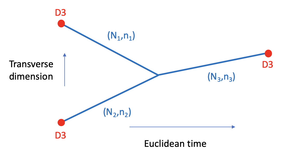
In the limit that $R_{9}/l_{p}\to 0$, the matrix model reduces to weakly coupled IIA string theory. It was argued that the matrix string gives rise to string perturbation theory in [32, 20], which reproduces the gravity three point function, see also [33, 34, 35]. In this paper, we argue that this is indeed the case for all values of the coupling, or all values of $R_{9}/l_{p}$, enabling us to access the eleven dimensional limit $R_{9}\to\infty$.

This paper is organized as follows. In section 2, we write the two and three point amplitudes as determined by supersymmetry and Lorentz invariance. We rewrite the amplitudes in a few different ways so as to take them to a form that is most natural for the matrix model computation. In section 3, we recall a few facts about the matrix model, introduce the setup for our computation, and compute the three point amplitude. Finally, we present some conclusions and discussion.

M-theory contains massless excitations that are in a short multiplet of the supersymmetry algebra. In fact, a massless particle preserves half of the supersymmetries, the ones that obey ${\not\!p}\epsilon=0$.

In order to describe the kinematic configuration of the three point amplitude, it is convenient to select four of the eleven dimensions and introduce the following coordinates

$$\begin{split}&ds^{2}=-2dx^{+}dx^{-}+2dzd\bar{z}~{},\\ &~{}~{}\textrm{where}~{}~{}~{}\sqrt{2}z=x^{9}+ix^{8},~{}~{}\sqrt{2}\bar{z}=x^{9}-ix^{8},~{}~{}\sqrt{2}x^{\pm}=x^{0}\pm x^{10}\ .\end{split}$$

(1)

We can now choose a configuration with momenta that are purely in the $p_{-}$ and $p_{z}$ directions, with $p_{+}=p_{\bar{z}}=0$ for all particles. This is possible only if the momenta in the direction $p_{8}$ are purely imaginary. For example, one possible configuration is

$$p^{i}_{\mu}=(p_{+},p_{-},p_{z},p_{\bar{z}})~{},~{}~{}~{}~{}p^{1}_{\mu}=(0,p^{1}_{-},q_{z},0)~{},~{}~{}~{}~{}p^{2}_{\mu}=(0,p^{2}_{-},-q_{z},0)~{},~{}~{}~{}~{}p^{3}_{\mu}=-(0,p^{1}_{-}+p^{2}_{-},0,0)$$

(2)

which clearly obeys momentum conservation. In addition, imposing ${{\not\!p}}^{i}\epsilon=0$ for the three particles $i=1,2,3$ implies that $\Gamma^{-}\epsilon=\Gamma^{z}\epsilon=0$, which are compatible conditions that select 1/4 of the 32 original supersymmetries.²²2This means that out of the 32 supersymmetric Ward identities [36] that we have for generic on-shell amplitudes only 24 linearly independent ones remain for the three point amplitude.

In order to write the scattering amplitudes, it is convenient to use an efficient description for the whole supermultiplet. Since any on-shell three point amplitude configuration can be related by Lorentz symmetry to one where the momenta are in four of the dimensions, as in (2), we will use four dimensional notation for the supersymmetries. This is the same notation that is used in describing ${\cal N}=8$ supergravity in four dimensions. In that case, it is convenient to use spinor helicity variables to write the momenta as $p_{\alpha\dot{\beta}}=\lambda_{\alpha}\bar{\lambda}_{\dot{\beta}}$. The supercharges obey an algebra of the form

$$\{Q_{\alpha},\bar{Q}_{\dot{\beta}}\}=\lambda_{\alpha}\bar{\lambda}_{\dot{\beta}}$$

(3)

and we can generate the whole multiplet by starting from the positive helicity graviton and writing [37, 38, 39, 40]

$$|\bar{\eta}\rangle=e^{b^{\dagger I}\bar{\eta}_{I}}|+\rangle~{},~{}~{}~{}~{}~{}{\rm with}~{}~{}~{}~{}~{}b^{\dagger I}\equiv\bar{w}^{\dot{\beta}}\bar{Q}_{\dot{\beta}}^{\,I}$$

(4)

where $\bar{w}$ and $w$ are spinors obeying³³3 Note that $[\bar{w},\bar{\lambda}]$ denotes a “square bracket” defined as in (4) and not a commutator.

$$[\bar{w},\bar{\lambda}]\equiv{\bar{w}}^{\dot{\beta}}\bar{\lambda}_{\dot{\beta}}=1~{},~{}~{}~{}~{}~{}~{}~{}~{}~{}\langle w,\lambda\rangle=w^{\alpha}\lambda_{\alpha}=1\ .$$

(5)

In (4) $I$ runs over eight values. This implies that $b^{\dagger I}$ in (4) and $b_{I}\equiv w^{\alpha}Q_{\alpha I}$ are canonically normalized fermion creation and annihilation operators obeying $\{b_{I},b^{\dagger I^{\prime}}\}=\delta_{I}^{I^{\prime}}$ thanks to (3) and (5).

Using this notation, the two point amplitude is

$${\cal A}_{2}=-2p_{-}(2\pi)^{10}\delta(p_{-}+p^{\prime}_{-})\delta^{9}(\vec{p}+\vec{p}^{\prime})\delta^{8}(\bar{\eta}_{I}+\bar{\eta^{\prime}}_{I})$$

(6)

(note that there is no $\delta(p_{+}+p_{+}^{\prime})$ term). This sets the normalization of the states.

For the three point amplitude, we will consider a configuration where all $\bar{\lambda}^{i}$ are proportional to each other⁴⁴4The other amplitude is similar up to exchanging the bar and unbarred quantities [41], and we will not discuss it any further in this paper.

$${\cal A}_{3}=\sqrt{16\pi G_{N,11}}\sqrt{2}(2\pi)^{11}\delta(\sum p_{-}^{i})\delta(\sum p_{+}^{i})\delta^{9}(\sum\vec{p}^{\,i})\delta^{16}(\lambda_{\alpha}^{i}\bar{\eta}_{I}^{i}){1\over\left(\langle 1,2\rangle\langle 2,3\rangle\langle 1,3\rangle\right)^{2}}$$

(7)

This form of the amplitude is completely determined by supersymmetry and Lorentz invariance. In particular, supersymmetry fixes the sixteen delta functions in (7). This is, of course, the amplitude in the gravity theory, but it is also the amplitude in the full M-theory because symmetries fully fix it up to an overall constant. Here we fixed the overall constant by computing it in gravity [42].

We first review the BFSS model and emphasize some aspects that will be important in later computations. The BFSS matrix model is defined by

$$S={1\over R_{-}}\int dt\textrm{Tr}\left[{1\over 2}\sum_{a=1}^{9}(D_{t}X^{a})^{2}+{1\over 4}{R_{-}^{2}\over(2\pi)^{2}l_{p}^{6}}\sum_{a,b=1}^{9}[X^{a},X^{b}]^{2}+{\rm fermions}\right]$$

(31)

where $t=x^{+}$, and $X^{a}$ are normalized so that they are matrix versions of the position coordinates, with dimensions of length. The matrices are $N\times N$ in the adjoint of the $U(N)$ gauge group [2, 44]. The fermions are in the 16 of SO(9). We also used that $G_{N,11}=16\pi^{7}l_{p}^{9}$.

The $U(1)$ part of the theory decouples and describes the center of mass degrees of freedom, which consist of nine positions and 16 Majorana fermions. These fermions are the Goldstone fermions of the 16 supercharges that are not preserved by a massless superparticle with null momentum. The physics of these nine variables and 16 fermions reproduces what we expect for a superparticle in light cone gauge. In particular, they give rise to the two point amplitude (28) and the “center of mass” part of the three point amplitude. We will discuss this in more detail below. The $SU(N)$ degrees of freedom are believed to give rise to a zero energy bound state at threshold [45] as well as a continuum. The continuum is related to configurations where the matrices develop large diagonal vacuum expectation values that break $U(N)\to\prod_{i=1}^{\ell}U(N_{i})$ which are then viewed as a scattering state of $\ell$ gravitons with null momentum $-p_{-}^{i}=N_{i}/R_{-}$. Each of these $U(N_{i})$ factors has a $U(1)_{i}$ part and an $SU(N_{i})$ part. When we define the asymptotic scattering states we focus on the zero energy bound state in the $SU(N_{i})$ parts. Then the $U(1)_{i}$ parts describe massless superparticles.

The 32 original supersymmetries are still realized in this theory: 16 of them linearly and 16 non-linearly. The latter are realized as shifts of the 16 Majorana fermions of the $U(1)$ part of the theory. The quantization of these sixteen fermions in each $U(1)$ fills out the $2^{8}$ states of a massless superparticle in eleven dimensions. We can use the same method as in (4) to label the asymptotic states in terms of Grassmann variables. This means that we can define a matrix model amplitude, in canonical normalization, in terms of scattering states ${\cal A}_{MM}^{c}$. The BFSS conjecture [2] states that the large $N$ limit of these amplitudes, keeping $-p^{i}_{-}=N_{i}/R_{-}$ fixed, precisely matches the M-theory amplitudes with $x^{-}$ non-compact.

The matrix model does not realize the full super-Poincare symmetry, but it does realize a subgroup of these symmetries. This subgroup is constraining enough to fix the full polarization dependence of the three point amplitude. To see this, first note that, for the three point amplitude, we can use rotation symmetry, momentum conservation and Galilean symmetry (which is a part of the original Lorentz group that commutes with $x^{-}$ translations) to transform to a momentum configuration that lies in just four of the eleven dimensions. This justifies our use of four dimensional notation. This is completely parallel to our discussion of the M-theory amplitude. The only new point is that we do not need to use the broken boosts that involve the $x^{-}$ coordinate, the boosts that would change $N_{i}$.

The next observation is that the algebra of the supercharges is not modified relative to the non-compact situation. In other words, the supercharge algebra acting on the external states is the same as in (3). All the various polarization states can be obtained by the action of the same operators discussed in (4) and (5). In the matrix model, the $b_{I}$ and $b^{\dagger I}$ are the fermionic creation and annihilation operators for each $U(1)_{i}$ factor [46]. Once we combine the various polarization states into a field as in (4), we can then view the supercharges as acting as

$$Q_{\alpha I}=\sum_{i}\lambda^{i}_{\alpha}\bar{\eta}_{I}^{i}~{},~{}~{}~{}~{}~{}~{}\bar{Q}_{\dot{\beta}}^{I}=\sum_{i}\bar{\lambda}^{i}_{\dot{\beta}}\partial_{\bar{\eta}^{i}_{I}}\ .$$

(32)

For three point kinematics, equation (32) gives us the action of only half of the $\bar{Q}$ supersymmetries. However, this is sufficient because the three point function is actually invariant under the other half. We now try to write the most general Grassman expression for the the three point function that will be invariant under (32):

$$\delta^{16}(\sum_{i}\lambda^{i}_{\alpha}\bar{\eta}_{I}^{i})\ .$$

(33)

In principle, equation (33) could be multiplied by an extra function of the $\bar{\eta}^{i}_{I}$. However, for the three point function, there is no function we can add that is non-zero on the support of the delta function (33) which is invariant under the $\bar{Q}$ supersymmetries in (33). Of course, (33) is invariant due to momentum conservation. This means that (33) is the only combination that is invariant under supersymmetry. This determines completely the polarization dependence of the three point amplitude. Let us emphasize that despite the fact that we are using four dimensional notation, equation (33) encodes all the polarization data in the full eleven dimensional theory. In other words, the $\bar{\eta}_{I}$ variables have spin in the other 7 dimensions.

The conclusion is that the only unknown part of the three point amplitude is a function of the $N_{i}$. These cannot be changed by any of the symmetries that are realized in the matrix model. In other words, the three point amplitude in the matrix model is (7), up to an overall multiplicative function of the $N_{i}$. We will show that this function is a constant independent of the $N_{i}$, which we expect to be one, but we did not check the overall numerical value.

References

- [1] B. de Wit, J. Hoppe, and H. Nicolai, “On the Quantum Mechanics of Supermembranes,” Nucl. Phys. B 305, 545 (1988)
- [2] Tom Banks, W. Fischler, S. H. Shenker, and Leonard Susskind, “M theory as a matrix model: A Conjecture,” Phys. Rev. D 55, 5112–5128 (1997), arXiv:hep-th/9610043
- [3] Leonard Susskind, “Another conjecture about M(atrix) theory,” (4 1997), arXiv:hep-th/9704080
- [4] Nathan Seiberg, “Why is the matrix model correct?.” Phys. Rev. Lett. 79, 3577–3580 (1997), arXiv:hep-th/9710009
- [5] Ashoke Sen, “D0-branes on T**n and matrix theory,” Adv. Theor. Math. Phys. 2, 51–59 (1998), arXiv:hep-th/9709220
- [6] Joseph Polchinski, “M theory and the light cone,” Prog. Theor. Phys. Suppl. 134, 158–170 (1999), arXiv:hep-th/9903165
- [7] Piljin Yi, “Witten index and threshold bound states of D-branes,” Nucl. Phys. B 505, 307–318 (1997), arXiv:hep-th/9704098
- [8] Savdeep Sethi and Mark Stern, “D-brane bound states redux,” Commun. Math. Phys. 194, 675–705 (1998), arXiv:hep-th/9705046
- [9] Gregory W. Moore, Nikita Nekrasov, and Samson Shatashvili, “D particle bound states and generalized instantons,” Commun. Math. Phys. 209, 77–95 (2000), arXiv:hep-th/9803265
- [10] Anatoly Konechny, “On asymptotic Hamiltonian for SU(N) matrix theory,” JHEP 10, 018 (1998), arXiv:hep-th/9805046
- [11] Massimo Porrati and Alexander Rozenberg, “Bound states at threshold in supersymmetric quantum mechanics,” Nucl. Phys. B 515, 184–202 (1998), arXiv:hep-th/9708119
- [12] Savdeep Sethi and Mark Stern, “Invariance theorems for supersymmetric Yang-Mills theories,” Adv. Theor. Math. Phys. 4, 487–501 (2000), arXiv:hep-th/0001189
- [13] Ying-Hsuan Lin and Xi Yin, “On the Ground State Wave Function of Matrix Theory,” JHEP 11, 027 (2015), arXiv:1402.0055 [hep-th]
- [14] Michael R. Douglas, Daniel N. Kabat, Philippe Pouliot, and Stephen H. Shenker, “D-branes and short distances in string theory,” Nucl. Phys. B 485, 85–127 (1997), arXiv:hep-th/9608024
- [15] Katrin Becker and Melanie Becker, “A Two loop test of M(atrix) theory,” Nucl. Phys. B 506, 48–60 (1997), arXiv:hep-th/9705091
- [16] Katrin Becker, Melanie Becker, Joseph Polchinski, and Arkady A. Tseytlin, “Higher order graviton scattering in M(atrix) theory,” Phys. Rev. D 56, R3174–R3178 (1997), arXiv:hep-th/9706072
- [17] Joseph Polchinski and Philippe Pouliot, “Membrane scattering with M momentum transfer,” Phys. Rev. D 56, 6601–6606 (1997), arXiv:hep-th/9704029
- [18] Jan C. Plefka, Marco Serone, and Andrew K. Waldron, “The Matrix theory S matrix,” Phys. Rev. Lett. 81, 2866–2869 (1998), arXiv:hep-th/9806081
- [19] Washington Taylor, “D-brane field theory on compact spaces,” Phys. Lett. B 394, 283–287 (1997), arXiv:hep-th/9611042
- [20] Robbert Dijkgraaf, Erik P. Verlinde, and Herman L. Verlinde, “Matrix string theory,” Nucl. Phys. B 500, 43–61 (1997), arXiv:hep-th/9703030
- [21] Oren Bergman, “Three pronged strings and 1/4 BPS states in N=4 superYang-Mills theory,” Nucl. Phys. B 525, 104–116 (1998), arXiv:hep-th/9712211
- [22] Oren Bergman and Barak Kol, “String webs and 1/4 BPS monopoles,” Nucl. Phys. B 536, 149–174 (1998), arXiv:hep-th/9804160
- [23] John H. Schwarz, “Lectures on superstring and M theory dualities: Given at ICTP Spring School and at TASI Summer School,” Nucl. Phys. B Proc. Suppl. 55, 1–32 (1997), arXiv:hep-th/9607201
- [24] Ofer Aharony and Amihay Hanany, “Branes, superpotentials and superconformal fixed points,” Nucl. Phys. B 504, 239–271 (1997), arXiv:hep-th/9704170
- [25] Ofer Aharony, Amihay Hanany, and Barak Kol, “Webs of (p,q) five-branes, five-dimensional field theories and grid diagrams,” JHEP 01, 002 (1998), arXiv:hep-th/9710116
- [26] Keshav Dasgupta and Sunil Mukhi, “BPS nature of three string junctions,” Phys. Lett. B 423, 261–264 (1998), arXiv:hep-th/9711094
- [27] Ashoke Sen, “String network,” JHEP 03, 005 (1998), arXiv:hep-th/9711130
- [28] Barak Kol, “Thermal monopoles,” JHEP 07, 026 (2000), arXiv:hep-th/9812021
- [29] Shamik Banerjee, Ashoke Sen, and Yogesh K. Srivastava, “Partition Functions of Torsion 1 Dyons in Heterotic String Theory on T**6,” JHEP 05, 098 (2008), arXiv:0802.1556 [hep-th]
- [30] Ashoke Sen, “Wall Crossing Formula for N=4 Dyons: A Macroscopic Derivation,” JHEP 07, 078 (2008), arXiv:0803.3857 [hep-th]
- [31] Ashoke Sen, “BPS Spectrum, Indices and Wall Crossing in N=4 Supersymmetric Yang-Mills Theories,” JHEP 06, 164 (2012), arXiv:1203.4889 [hep-th]
- [32] Lubos Motl, “Proposals on nonperturbative superstring interactions,” (1 1997), arXiv:hep-th/9701025
- [33] Steven B. Giddings, Feike Hacquebord, and Herman L. Verlinde, “High-energy scattering and D pair creation in matrix string theory,” Nucl. Phys. B 537, 260–296 (1999), arXiv:hep-th/9804121
- [34] G. Bonelli, L. Bonora, and F. Nesti, “String interactions from matrix string theory,” Nucl. Phys. B 538, 100–116 (1999), arXiv:hep-th/9807232
- [35] G. Bonelli, L. Bonora, F. Nesti, and Alessandro Tomasiello, “Matrix string theory and its moduli space,” Nucl. Phys. B 554, 103–135 (1999), arXiv:hep-th/9901093
- [36] Marcus T. Grisaru and H. N. Pendleton, “Some Properties of Scattering Amplitudes in Supersymmetric Theories,” Nucl. Phys. B 124, 81–92 (1977)
- [37] V. P. Nair, “A Current Algebra for Some Gauge Theory Amplitudes,” Phys. Lett. B 214, 215–218 (1988)
- [38] Edward Witten, “Perturbative gauge theory as a string theory in twistor space,” Commun. Math. Phys. 252, 189–258 (2004), arXiv:hep-th/0312171
- [39] Massimo Bianchi, Henriette Elvang, and Daniel Z. Freedman, “Generating Tree Amplitudes in N=4 SYM and N = 8 SG,” JHEP 09, 063 (2008), arXiv:0805.0757 [hep-th]
- [40] Nima Arkani-Hamed, Freddy Cachazo, and Jared Kaplan, “What is the Simplest Quantum Field Theory?.” JHEP 09, 016 (2010), arXiv:0808.1446 [hep-th]
- [41] Nima Arkani-Hamed and Jared Kaplan, “On Tree Amplitudes in Gauge Theory and Gravity,” JHEP 04, 076 (2008), arXiv:0801.2385 [hep-th]
- [42] Bryce S. DeWitt, “Quantum Theory of Gravity. 2. The Manifestly Covariant Theory,” Phys. Rev. 162, 1195–1239 (1967)
- [43] Yu-tin Huang, “Non-Chiral S-Matrix of N=4 Super Yang-Mills,” (4 2011), arXiv:1104.2021 [hep-th]
- [44] Washington Taylor, “Lectures on D-branes, gauge theory and M(atrices),” in 2nd Trieste Conference on Duality in String Theory (1997) pp. 192–271, arXiv:hep-th/9801182
- [45] Edward Witten, “Bound states of strings and p-branes,” Nucl. Phys. B 460, 335–350 (1996), arXiv:hep-th/9510135
- [46] Jan Plefka and Andrew Waldron, “On the quantum mechanics of M(atrix) theory,” Nucl. Phys. B 512, 460–484 (1998), arXiv:hep-th/9710104
- [47] W. Nahm, “A Simple Formalism for the BPS Monopole,” Phys. Lett. B 90, 413–414 (1980)
- [48] Duiliu-Emanuel Diaconescu, “D-branes, monopoles and Nahm equations,” Nucl. Phys. B 503, 220–238 (1997), arXiv:hep-th/9608163
- [49] Ignatios Antoniadis, E. Gava, K. S. Narain, and T. R. Taylor, “Topological amplitudes in string theory,” Nucl. Phys. B 413, 162–184 (1994), arXiv:hep-th/9307158
- [50] Luis F. Alday and Juan Maldacena, “Comments on gluon scattering amplitudes via AdS/CFT,” JHEP 11, 068 (2007), arXiv:0710.1060 [hep-th]
- [51] Steven Weinberg, “Infrared photons and gravitons,” Phys. Rev. 140, B516–B524 (1965)
- [52] Freddy Cachazo and Andrew Strominger, “Evidence for a New Soft Graviton Theorem,” (4 2014), arXiv:1404.4091 [hep-th]
- [53] Aidan Herderschee and Juan Maldacena, “Soft Theorems in Matrix Theory,” (12 2023), arXiv:2312.15111 [hep-th]
- [54] Tom Banks and Lubos Motl, “Heterotic strings from matrices,” JHEP 12, 004 (1997), arXiv:hep-th/9703218
- [55] Lubos Motl and Leonard Susskind, “Finite N heterotic matrix models and discrete light cone quantization,” (8 1997), arXiv:hep-th/9708083
- [56] Ruth Britto, Freddy Cachazo, Bo Feng, and Edward Witten, “Direct proof of tree-level recursion relation in Yang-Mills theory,” Phys. Rev. Lett. 94, 181602 (2005), arXiv:hep-th/0501052
- [57] Yuhma Asano, Goro Ishiki, and Shinji Shimasaki, “Emergent bubbling geometries in gauge theories with SU(2—4) symmetry,” JHEP 09, 137 (2014), arXiv:1406.1337 [hep-th]
- [58] Yuhma Asano, Goro Ishiki, Takashi Okada, and Shinji Shimasaki, “Exact results for perturbative partition functions of theories with SU(2—4) symmetry,” JHEP 02, 148 (2013), arXiv:1211.0364 [hep-th]
- [59] David Eliecer Berenstein, Juan Martin Maldacena, and Horatiu Stefan Nastase, “Strings in flat space and pp waves from N=4 superYang-Mills,” JHEP 04, 013 (2002), arXiv:hep-th/0202021