Slepian Beamforming: Broadband Beamforming using Streaming Least Squares

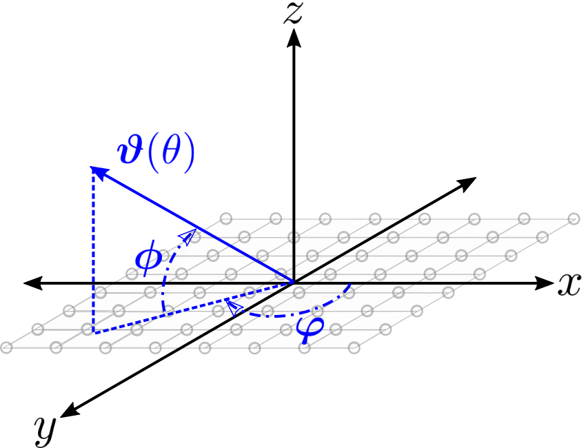
The array has $M$ elements with positions $\boldsymbol{p}_{1},\ldots,\boldsymbol{p}_{M}$ relative to the array origin. The framework we develop can be applied to arbitrary arrays in 3D, though of course the effectiveness of the methods we propose will depend on the configuration of the elements inside the aperture (something that is true for any array processing algorithm). Most of our numerical experiments are for uniform linear and uniform planar arrays with “$\lambda/2$” spacing, where $\lambda=c/f_{c}$ and $c$ is the speed of light.

Adjusting the time axis so that the array center observes $s_{\mathrm{mod}}(t)$, the modulated signal at element $m$ will be

$$y_{\mathrm{mod},m}(t)=s_{\mathrm{mod}}(t-\tau_{m}(\theta))~{}+~{}\text{corruption},\quad\text{where}~{}~{}\tau_{m}(\theta)=\boldsymbol{p}_{m}^{\mathrm{T}}\boldsymbol{\vartheta}(\theta)/c,\quad\boldsymbol{\vartheta}(\theta)=\begin{bmatrix}\cos\varphi\cos\phi\\ \sin\varphi\cos\phi\\ \sin\phi.\end{bmatrix}.$$

Demodulating the signal at every element gives us the observational model

$$y_{m}(t)=e^{-j2\pi f_{c}t}y_{\mathrm{mod},m}(t)=e^{-j2\pi f_{c}\tau_{m}(\theta)}s(t-\tau_{m}(\theta))~{}+~{}\text{corruption}.$$

(1)

Thus sampling the demodulated array outputs gives us (noisy) samples of $s(t)$ multiplied by known phases.

We will collect samples off all array elements simultaneously at times $t_{1},\ldots,t_{N}$ ($N$ will vary throughout the paper). The collection of array output at a fixed sampling time

$$\boldsymbol{y}[n]=\begin{bmatrix}y_{1}(t_{n})\\ \vdots\\ y_{M}(t_{n})\end{bmatrix},$$

(2)

is called a snapshot. For exposition, we will assume for most of the paper that the $t_{n}$ are uniformly spaced and are at (or above) the Nyquist rate for a $\Omega$-bandlimited signal. The formulation extends easily, however, to situations where the samples are taken at different times at each element and/or are non-equispaced in time. In Section 6 we will also discuss situations where our framework is effective even when the samples are observed through dimensionality reducing measurements.

The collection of snapshots $\{\boldsymbol{y}[n]\}_{n=1}^{N}$ give us information about $s(t)$ over a finite time interval; each sample can be interpreted as a linear measurement of $s(t)$. We thus treat the estimation of $s(t)$, the beamforming in direction $\theta$, as a linear inverse problem and solve it using least-squares. The output of the beamformer is a stream of Nyquist samples for the estimated signal.

We will approach the problem in two different ways. We will begin in Sections 3 and 4 with static batch estimation where we collect samples over an interval of time and then produce a signal estimate over the same time interval. In Section 5, we show how the least-squares solver can be implemented online to produce an estimate of arbitrary length. Key to both of these approaches is the Slepian representation for bandlimited signals over finite intervals of time which we review in Section 2. Section 6 extends these methods to estimating signals from snapshots that have been linearly encoded across space and time.

The observational model described by (1) and (2) can give us a qualitative understanding of what differentiates the narrowband and broadband cases. Roughly speaking, in the narrowband case the snapshots will be far apart in time (relative to the bandwidth of the signal) with each snapshot essentially containing information about a single Nyquist sample of $s(t)$. The array samples in each snapshot can then be coherently combined (usually by phase shifting and summing) independently into estimates of individual samples of $s(t)$. In the broadband case, the snapshots overlap with one another; each snapshot contains information about multiple Nyquist samples of $s(t)$ and each Nyquist samples influences multiple snapshots. Solving the least-squares problem accounts for this in an optimal way.

These two different situations are illustrated in Figure 2. In Figure 2(a), we show a narrowband signal being sampled at an array. The signal has bandwidth $\Omega=10$ MHz and was modulated to a carrier frequency $f_{c}=5$ GHz. It was incident at angle of incidence $\theta=(\varphi,\phi)=(30^{\circ},10^{\circ})$ on a $4\times 4$ uniform planar array with spacing $c/2f_{c}$ matched to the carrier frequency and three snapshots were taken at the Nyquist rate $T_{s}=1/2\Omega=50$ ns. Each snapshot corresponds to a tight cluster of samples, we zoom in on the cluster for $n=3$ in Figure 2(b). The length of the time interval that each snapshot covers is

$$T_{1}(\theta)=\max_{m}\tau_{m}(\theta)-\min_{m}\tau_{m}(\theta),$$

(3)

which for this array geometry works out to $T_{1}(\theta)\approx 0.4$ ns $\ll T_{s}$. We are plotting the $\boldsymbol{y}[n]$ here without the phases $e^{-j2\pi f_{c}\tau_{m}(\theta)}$ from (1), so the signal is close to being a constant over the snapshot time $T_{1}(\theta)$. Each cluster can thus be coherently combined into an estimate of a single Nyquist sample of the underlying waveform just as is done in conventional narrowband beamforming.

A broadband example is shown in Figure 2(c). Here we generated a signal with $\Omega=5$ GHz, $f_{c}=10$ GHz and took $N=3$ snapshot of array samples as in (1)-(2) for a $4\times 4$ uniform planar array with elements spaced at half-wavelength $c/2f_{c}$m and the same angle of incidence $(30^{\circ},10^{\circ})$ as above. In this case, the length of the time interval for a single snapshot $T_{1}(\theta)=\max_{m}\tau_{m}(\theta)-\min_{m}\tau_{m}(\theta)\approx 0.2$ns exceeds the Nyquist sampling interval $T_{s}=0.1$ns by about a factor of $2$. As such, the snapshots, each of which consists of $16$ samples, exhibit significant overlap; the snapshot for $n=1$ is shown in blue, $n=2$ in red, and $n=3$ in yellow.

The snapshot overlap in the preceding example is actually mild. For example, one of our numerical experiments in Section 3.2 below uses a $32\times 32$ uniform planar array with $\Omega=5$ GHz and $f_{c}=20$ GHz. With the same angle of arrival as before, we have $T_{1}(\theta)\approx 1.04$ ns which is a factor of $10$ larger than $T_{s}=0.1$ ns, meaning that consecutive snapshot have about $90\%$ overlap.

As we can see from these examples, the quantities $T_{s}$ and $T_{1}(\theta)$ give us a natural way to decide if we are in the broadband or narrowband scenarios. We can safely use narrowband beamforming when $T_{1}(\theta)\ll T_{s}$ (so $2\Omega T_{1}(\theta)\ll 1$) for all angles of arrive $\theta$ of interest; we are plainly in the broadband scenario when $T_{1}(\theta)\geq T_{s}$ (so $2\Omega T_{1}(\theta)\geq 1$) for some $\theta$ of interest. Setting an exact threshold for $2\Omega T_{1}(\theta)$ to differentiate the two cases depends on our tolerance for error in approximating the $\{s_{m}(t-\tau_{m}(\theta))\}_{m=1}^{M}$ as a constant. More precise guidelines are discussed in Section 2 below.

We close this section by reiterating that the notion of broadband in our context does depend on the angle of incidence, especially on the elevation $\phi$. For $\phi\approx 0$ (meaning the signal is arriving “broadside”), the samples will always be clustered as in Figure 2(a), and in fact for $\phi=0$ all of the $\tau_{m}(\theta)$ will be equal to one another and $T_{1}(\theta)=0$. The methodology we present below, however, adapts naturally to these cases.

The standard beamforming model for both the narrowband and broadband case is concisely over-viewed in [1]. The narrowband case, which this paper does not focus on, takes the form of a weight and sum of sensor outputs. The classically stated condition for the narrowband assumption to hold is that the bandwidth should be small enough for signals received at any point across the array aperture to remain correlated to each other[2]. Though related, this a different condition than we formally state in Section 2. We define the broadband regime to be the point where the subspace dimension required to meet an approximation threshold exceeds one, and the dimension is a function of the signal’s time-bandwidth product.

The typical broadband (sometimes termed wideband) beamformer manifests as a set of tapped delay line filters attached to the sensor outputs. A popular assumption is that that the signal has been “pre-steered” e.g. the temporal offsets between sensors for a fixed direction of arrival have been compensated [3, Chap. 6]. This is generally achieved through true time-delay or fractional-delay filtering. Post pre-steering the filters are designed to combine channels in a manner that optimally filters noise and nulls interferers. The Frost beamformer [4] is a popular time-domain implementation of a “mininum variance distortionless response” (MVDR) beamformer that explicitly leverages pre-steering in its model. It is the time domain extension of Capon beamforming, which in its original formulation is a frequency domain approach [5]. As a general statement, essentially every broadband beamformer has complimentary frequency and time domain implementations. However, their respective performance do not substantially differ [6]. Our methodology distinguishes itself from these by requiring no notion of pre-steering.

The Frost/MVDR beamformer can be seen as a special case of a broader class of “linearly constrained minimum variance” (LCMV) beamformers [7, Chap. 2], the main distinction being that the latter in general do not use pre-steering. The fractional delay filtering portion of the optimal filter design is wrapped into the optimzation program through linear constraints. Though this is often done by spectrally sampling the passband, [8] implicitly proposed using Slepian basis vectors to form constraints. Several other works [9, 10, 11] examine the performance of tapped-delay line filter based methods with respect to the number of taps. The main focus being how to determine the minumum number of taps required in order to meet certain performance thresholds as a function of the array geometry and bandwidth. Perhaps most similar to our Slepian based MVDR [12] explicitly uses Slepian spaces to form a multi-channel output. However, the approach only considers a single snapshot’s Slepian space and is mainly focused on robustness to DOA estimation errors. Though we constrain and null our Slepian subspace based methods in a manner similar to these optimal methods, ultimately it is not a filter based approach.

Actually implementing tapped delay lines can be difficult and costly. To circumvent this [13, 14, 15] propose “sensor delay lines” as a method for practically implementing filters. In this paradigm a standard sensor array has a series of additional sensors placed behind it, increasing the array dimension. These additional sensors receive the signal at different times due to the spatial offset, and act as a tap in the standard filtering paradigm. The design process is essentially the same as before, with the main difference being that instead obtaining samples with temporal offsets via a delay line the signal is spatially sampled at the desired offsets.

Frequency invariant beamforming is a relatively modern approach to broadband beamforming. It is powerful because it allows us to directly map a narrowband beampattern (and all our intuition behind it) to a broadband filter bank [16, 17]. The method takes a target beam (generally a narrowband beam pattern), and carefully applies a non-linear map that shifts and dilates the target beam frequency response. Mapping this back into the time domain produces a filter bank that will generate the desired beam response across a wide variety of frequencies. A shortcoming of this design methodology is that it attenuates energy at lower frequencies [7, Chap. 5]. Hence if the signals energy is dispersed across the entire sampled band the frequency invariant beamformer will induce distortion. Again, our approach is not filter based, and furthermore does not attenuate low frequencies.

Subarray beamforming [18] decomposes the beamforming process into two parts. The operations are chosen such that the first part is generally suitable for analog processing while the second is generally suitable for digitial processing. In the broadband regime the full array is split into subarrays and narrowband beamformed on the subarrays. The ouput of the subarrays is then broadband beamformed [19]. The benefit being the true time delays required to broadband beamform only needs to be applied to the subarray outputs, reducing the number of true time delays the system requires. Performance depends on the size and shape of the subarray, with [20, 21, 22] examining different partitioning methods. These principles can be extended to optimal beamforming as discussed in [23]. We note that the basic principle of subarray beamforming is similar to the hybrid beamforming concepts used in MIMO communications [24], albeit in a more general context. As will be shown explicitly in Section 3.3 we can extend our method to the subarray setting, but again we do so without filtering.

The overarching feature distinguishing our method from all of the described existing approaches is the fact we do not use filters. Fundamentally, filters map blocks of snapshots to a single point whereas our approach maps blocks of snapshots to several points. It does this by successively fitting a robust subspace model to the sample blocks, essentially replacing the application of a filter with vector matrix multiplies. Throughout this paper we provide numerical experiments that compare our method against those mentioned above in a variety of scenarios. Through these results, it is shown that our formulation has the potential to yield substantial performance improvements over existing approaches.

Suppose we collect $N$ snapshots off of an $M$ element array. As discussed above, these samples contain information about the signal in a time interval of length $T_{N}(\theta)$ (we will simply take this interval to be $[0,T_{N}(\theta)]$ for the exposition below). It is clear that the mapping from the signal $s(t)$ to the array samples is linear. As such, we will treat the estimation of $s(t)$ as a linear inverse problem. Since

$$s(t)\approx\sum_{k=1}^{D_{N}(\theta)}\alpha_{k}\psi_{k}(t),$$

(9)

where the $\{\psi_{k}\}$ are the Slepian functions discussed in Section 2, we will estimate $s(t)$ by estimating the first (8) expansion coefficients $\{\alpha_{k}\}$. With this discretization of $s(t)$ in place, we now have a “forward model” for a sample snapshot (2),

$$\boldsymbol{y}[n]=\boldsymbol{A}_{n}(\theta)\boldsymbol{\alpha}+\text{corruption},$$

(10)

where $\boldsymbol{A}_{n}(\theta)$ is a $M\times D_{N}(\theta)$ matrix with entries

$$A_{n}(\theta)[m,k]=e^{-j2\pi f_{c}\tau_{m}(\theta)}\psi_{k}(t_{n}-\tau_{m}(\theta)).$$

Stacking the $N$ snapshots together with their corresponding forward models into $\underline{\boldsymbol{y}}$ and $\boldsymbol{A}(\theta)$,

$$\underline{\boldsymbol{y}}=\begin{bmatrix}\boldsymbol{y}[1]\\ \vdots\\ \boldsymbol{y}[N]\end{bmatrix},\quad\boldsymbol{A}(\theta)=\begin{bmatrix}\boldsymbol{A}_{1}(\theta)\\ \vdots\\ \boldsymbol{A}_{N}(\theta)\end{bmatrix},$$

(11)

we can now estimate the Slepian coefficients by solving the least-squares problem

$$\operatorname*{\text{minimize}}_{\boldsymbol{\alpha}\in\mathbb{C}^{D_{N}(\theta)}}~{}\frac{1}{2}\|\underline{\boldsymbol{y}}-\boldsymbol{A}(\theta)\boldsymbol{\alpha}\|_{2}^{2}+\delta\|\boldsymbol{\alpha}\|_{2}^{2}.$$

(12)

The $\delta>0$ above is a regularization parameter that can be set depending on the structure of the singular values of $\boldsymbol{A}(\theta)$; we will see below that $\boldsymbol{A}(\theta)$ is in general fairly well conditioned and so we can typically take $\delta=0$. With $\delta=0$, the closed form solution to (12) is

$$\widehat{\boldsymbol{\alpha}}=\boldsymbol{A}(\theta)^{\dagger}\underline{\boldsymbol{y}}=\boldsymbol{V}(\theta)\boldsymbol{\Sigma}(\theta)^{-1}\boldsymbol{U}(\theta)^{\mathrm{H}}\underline{\boldsymbol{y}},$$

(13)

where $\boldsymbol{A}(\theta)=\boldsymbol{U}(\theta)\boldsymbol{\Sigma}(\theta)\boldsymbol{V}(\theta)^{\mathrm{H}}$ is the singular value decomposition of $\boldsymbol{A}(\boldsymbol{\theta})$.

Given $\widehat{\boldsymbol{\alpha}}$, we can reconstruct any set of samples we like using another linear map. For example, if we want to estimate $s(t)$ at $t_{1},\ldots,t_{N}$, we simply form the $N\times D_{N}(\theta)$ matrix $\boldsymbol{\Psi}$ with entries $\Psi[n,d]=\psi_{d}(t_{n})$ and compute $\widehat{}\underline{\boldsymbol{s}}=\boldsymbol{\Psi}\widehat{\boldsymbol{\alpha}}$. Note that the entire mapping from array samples $\underline{\boldsymbol{y}}$ to samples $\underline{\boldsymbol{s}}$ of the beamformed signal can be collapsed into a single matrix, $\underline{\boldsymbol{s}}=\boldsymbol{\Psi}\boldsymbol{A}(\theta)^{\dagger}\underline{\boldsymbol{y}}=:\boldsymbol{W}(\theta)\underline{\boldsymbol{y}}$. The rows of $\boldsymbol{W}(\theta)$ can be interpreted as “weights” that combine array samples across space and time into an estimate of a sample of $s(t)$. This concept will be discussed with great detail in Section 6.

Once we have formalized the forward model (10) and the Slepian discretization (9), the least-squares approach to estimation in (12) is straightforward and natural. It it also, as we will show with numerical experiments in the next section, extremely effective as it outperforms both classical and recently developed methods for broadband beamforming while being no more expensive computationally.

As a first demonstration of the effectiveness of our method this we compare its performance to more standard paradigms. We examine two test cases, the first being the $32\times 32$ element UPA described in Section 2 where $f_{c}=20$ GHz, $\Omega=5$ GHz, and $\theta=(\pi/4,\pi/2)$. The second case is a 64-element uniform linear array (ULA) where $f_{c}=20$ GHz, $\Omega=5$ GHz, and $\theta=\pi/2$. For the ULA $d(\Omega T_{1}(\theta))=20$ meaning its spatial subspace dimension is slightly larger. In both cases we examine $N=2^{5}$ snapshots. To test the performance of various beamforming methods on these arrays we generate a random bandlimited signal using a sum-of-sinusoids model. The signal is then corrupted by complex Gaussian noise at a nominal SNR and impinges on the array as a plane wave. The signal is beamformed using one of the described methods and we observe the beamformed SNR. Results were averaged across 50 randomly generated trials.

In terms of conventional methods we compare against two versions of delay and sum beamforming. The first is the more traditional of the two and employs fractional delay filters to digitally align the signals in time (often termed pre-steering) prior to summing [3]. These fractional delay filters consist of sinc interpolators truncated to $R$ taps, where we note that as $R\to\infty$ the filters become ideal. Since performance varies drastically with the length of the filter we compare against several choices in $R$. We note that there are several methods of fractional delay interpolation that may offer better results than sinc interpolation. However, methods such a Lagrange or spline interpolation need some degree of oversampling to yield truly drastic improvement over sinc inteprolation. Since we are operating in a critically sampled regime, the difference amongst interpolation methods is limited and therefore we settle for the most intuitive method. The second version of delay and sum we examine is a frequency invariant beamformer, which uses a nonlinear map to generate a broadband filter bank that matches a narrowband response across a desired frequency band [16, 17]. In this case we map a Hann windowed narrowband response to the frequency invariant broadband regime.

The results for the ULA and UPA are shown in Figure 3(a) and 3(b) respectively, where the black line represents the ideal array gain of $M$. We note that this ideal gain can be achieved when the fractional delay filters are infinite in length, or a perfect true time delay can be applied. The results for both arrays follows a similar trend; at low SNRs the error is noise dominated and hence all methodologies perform similarly. The story changes as we increase the SNR. The error becomes dominated by the filter bias and we see a sharp performance roll off. Though increasing the filter size alleviates this effect to some extent, even for long filters the roll off is apparent.

Perhaps surprisingly, the frequency invariant beamformers yield comparatively poor performance. This is likely due to attenuation of lower frequency components, which is a known phenomena and discussed in detail in Appendix A. Essentially the filter design process has a limited ability to produce filters with good frequency invariance at low frequencies[16, 7]. Since we assume baseband processing, critical sampling, and the signal is evenly distributed across the band a substantial portion of the signals energy gets attentuated, leading to high distortion. However, if the signal was oversampled or its energy was concentrated only in the upper half of the band, then this style of beamforming would perform far better. A demonstration of the affects of oversampling on frequency invariant beamforming are provided in Appendix A.

Using our least squares approach we can formulate a natural extension to subarray beamforming. We begin this discussion with a brief introduction into the general concept of subarray beamforming. In the standard case the array is divided into multiple smaller arrays i.e., subarrays. More formally we break an $M$ element array into $M^{\prime}$ subarrays. The size of the subarrays is chosen to ensure the aperture is reduced to the point that the signal is narrowband as it lies across any particular subarray [20, 18]. Let $\mathcal{M}_{m^{\prime}}\subset\{1,\dots,M\}$ be the set containing the indices associated with the $m^{\prime}$th subarray. The signal is then narrowband beamformed with weights $\{w_{m}\}_{m=1}^{M}$ at the subarray level such that that a given sub-beam is

$\displaystyle y_{\mathrm{sub},m^{\prime}}(t)=\sum_{m\in{M}_{m^{\prime}}}w_{m}y_{m}(t).$

(14)

The temporal offset between sub-beams is traditionally corrected via filtering (or any suitable method) followed by summation to form the full beam. Some advantages of this is that it reduces the number of channels that must be filtered, and it splits the problem into operations that can naturally and respectively be handled in the analog and digital domain [24].

Given access to sub-beams instead of direct samples off the array changes our forward model such that (12) must be modified. The details of this modification are thoroughly overviewed in Section 6, but in general as long as $M^{\prime}>d(\Omega T_{1}(\theta))$ so that the spatial subspace dimension is sufficiently sampled, we can recover $\boldsymbol{\alpha}$ as accurately as if we had direct access to the $\underline{\boldsymbol{y}}$.

In the next section we display numerical experiments demonstrating that subarray Slepian subspace beamforming performs nearly as well as the full scaled version. Again our least squares approach outperforms conventional methods, and additionally shows less degradation in performance with the subarray size. The concepts put forth in this section, namely dimensionality reduction prior to coefficient estimation, will be generalized in Section 6 where subarray beamforming can be considered as a special case.

To see how subarray beamforming effects performance we return to the test cases presented in Section 3.2, with all parameters for the ULA and UPA remaining the same. We test two subarray partitionings for each geomery, with the ULA being split into $2\times 1$ and $4\times 1$ subarrays and the UPA being split into $2\times 2$ and $4\times 4$ subarrays. We again compare the Slepian subspace beamformer’s performance to delay and sum beamformers using fractional delay filters. For delay and sum, the subarrays are beamformed using standard complex phase weightings. Time delays are applied to the sub-beams using length $R=2^{6}$ sinc-interpolation filters.

Alongside both subarray configurations for both arrays the results shown in Figure 4 also contain the full scale (e.g. no subarrays) results as a point of comparison. The ULA results in Figure 4(a) show that in the $2\times 1$ subarray configuration there is almost no degradation in performance when using Slepian subspace beaforming and remains close to ideal. In contrast, delay and sum shows a faster performance roll off that is seen when operating at full scale. This roll-off becomes more pronounced in the $4\times 1$ case, which is due to the signal nearly breaking the broadband threshold at the subarray level. Hence the narrowband beamforming stage incurs more distortion prior to filtering. However, there is also a sharp roll off in the Slepian performance when we switch to a $4\times 1$ configuration. This is due to the fact that in this case $M^{\prime}=16$, meaning $M^{\prime}<d(\Omega T_{1}(\theta))=20$ and the spatial dimension is not sufficiently sampled.

In conclusion the experiments show that subarray Slepian subspace beamforming can perform nearly as well as the full array case when the number of subarrays is sufficient. Performance of delay and sum is largely tied to the size of the subarray, with sharp performance degradation occurring when the subarray aperture is too large regardless of the number of subarrays. Furthermore, even when the subarray aperture is small there is a far wider performance gap between the subarray and full array versions of delay and sum than in the Slepian case.

As our broadband beamformer is a least-squares solver, we can systematically analyze its performance. In this section, we characterize the performance of our least squares beamformer in (12) by showing how the bias and variance can be computed given the array geometry. We show that the bias is very small while the variance yields the same (optimal) array gain.

For our analysis, we will compute the expected mean-squared error of the beamformed estimate when the incoming (demodulated) signal $s(t)$ is a Gaussian random process with zero mean and a flat power spectrum on $[-\Omega,\Omega]$. The signal is normalized so that its total expected energy on the observation interval $[0,T_{N}(\theta)]$ is $\Omega T_{N}(\theta)$:

$$\int_{0}^{T_{N}(\theta)}\operatorname{E}[|s(t)|^{2}]~{}dt=\Omega T_{N}(\theta).$$

The signal then has a Slepian decomposition with random coefficients

$$s(t)=\sum_{k=1}^{\infty}\alpha_{k}\psi_{k}(t),\quad\alpha_{k}\sim\mathrm{Normal}(0,\lambda_{k}),$$

(15)

where the $\alpha_{k}$ are independent and $\lambda_{k}$ is the $k$th largest eigenvalue of the integral operator in (5). We observe $N$ array snapshots $\underline{\boldsymbol{y}}$ as in (11) in the presence of additive noise $\boldsymbol{\eta}$, a random vector with zero mean and covariance matrix $\sigma^{2}{\bf I}$ that is independent of $s(t)$. We will use the least-squares technique in the previous section (with $\delta=0$) with $D_{N}(\theta)$ chosen for an appropriately small choice of $\epsilon$.

References

- [1] B. Van Veen and K. Buckley, “Beamforming: a versatile approach to spatial filtering,” IEEE ASSP Mag., vol. 5, no. 2, pp. 4–24, 1988.
- [2] R. Compton, Adaptive Antennas: Concepts and Performance. Prentice-Hall, 1988.
- [3] H. V. Trees, Optimum Array Processing: Part IV of Detection, Estimation, and Modulation Theory. Wiley Interscience, 2002.
- [4] O. Frost, “An algorithm for linearly constrained adaptive array processing,” Proc. IEEE, vol. 60, no. 8, pp. 926–935, 1972.
- [5] J. Capon, “High-resolution frequency-wavenumber spectrum analysis,” Proc. IEEE, vol. 57, no. 8, pp. 1408–1418, 1969.
- [6] R. Compton, “The relationship between tapped delay-line and FFT processing in adaptive arrays,” IEEE Trans. Antennas Propag., vol. 36, no. 1, pp. 15–26, 1988.
- [7] W. Liu and S. Weiss, Wideband Beamforming: Concepts and Techniques. Wiley Publishing, 2010.
- [8] K. Buckley, “Spatial/Spectral filtering with linearly constrained minimum variance beamformers,” IEEE Trans. Acoust., Speech, Signal Process., vol. 35, no. 3, pp. 249–266, 1987.
- [9] J. Mayhan, A. Simmons, and W. Cummings, “Wide-band adaptive antenna nulling using tapped delay lines,” IEEE Trans. Antennas Propag., vol. 29, no. 6, pp. 923–936, 1981.
- [10] W. Rodgers and R. Compton, “Adaptive Array Bandwidth with Tapped Delay-Line Processing,” IEEE Trans. Aerosp. Electron. Syst., vol. AES-15, no. 1, pp. 21–28, 1979.
- [11] F. Vook and R. Compton, “Bandwidth performance of linear adaptive arrays with tapped delay-line processing,” IEEE Trans. Aerosp. Electron. Syst., vol. 28, no. 3, pp. 901–908, 1992.
- [12] A. Pezeshki, B. Van Veen, L. Scharf, H. Cox, and M. Nordenvaad, “Eigenvalue Beamforming Using a Multirank MVDR Beamformer and Subspace Selection,” IEEE Trans. Signal Process., vol. 56, no. 5, pp. 1954–1967, 2008.
- [13] N. Lin, W. Liu, and R. Langley, “Performance Analysis of a Broadband Beamforming Structure Without Tapped Delay-Lines,” in Int. Conf. on Digital Signal Process., July 2007.
- [14] W. Liu, “Adaptive Broadband Beamforming with Spatial-Only Information,” in Int. Conf. on Digital Signal Process., July 2007.
- [15] ——, “Adaptive wideband beamforming with sensor delay-lines,” Signal Process., vol. 89, no. 5, pp. 876–882, 2009.
- [16] W. Liu and S. Weiss, “Design of Frequency Invariant Beamformers for Broadband Arrays,” IEEE Trans. Signal Process., vol. 56, no. 2, pp. 855–860, 2008.
- [17] D. Ward, R. Kennedy, and R. Williamson, “Theory and design of broadband sensor arrays with frequency invariant far‐field beam patterns,” J. of the Acoust. Soc., vol. 97, no. 2, pp. 1023–1034, 1995.
- [18] U. Nickel, “Properties of Digital Beamforming with Subarrays,” in CIE Int. Conf. Radar, October 2006.
- [19] R. Mailloux, “Subarray technology for time delayed scanning arrays,” in IEEE Int. Conf. Microw., Commun., Antennas and Electron. Syst., November 2009.
- [20] U. Nickel, “Subarray configurations for digital beamforming with low sidelobes and adaptive interference suppression,” in Proc. Int. Radar Conf., May 1995.
- [21] R. Haupt, “Optimized Weighting of Uniform Subarrays of Unequal Sizes,” IEEE Trans. Antennas Propag., vol. 55, no. 4, pp. 1207–1210, 2007.
- [22] Z. Xiong, Z. Xu, S. Chen, and S. Xiao, “Subarray Partition in Array Antenna Based on the Algorithm X,” IEEE Antennas Wireless Propag. Lett., vol. 12, pp. 906–909, 2013.
- [23] Z. Xie, J. Zhu, C. Fan, and X. Huang, “An Improved Sub-Array Adaptive Beamforming Technique Based on Multiple Sources of Errors,” J. Marine Sci. and Eng., vol. 8, no. 10, 2020.
- [24] A. Molisch, V. Ratnam, S. Han, Z. Li, S. Nguyen, L. Li, and K. Haneda, “Hybrid Beamforming for Massive MIMO: A Survey,” IEEE Commun. Mag., vol. 55, no. 9, pp. 134–141, 2017.
- [25] D. Slepian and H. Pollak, “Prolate spheroidal wave functions, Fourier analysis and uncertainty I,” Bell Systems Tech. Journal, vol. 40, no. 1, pp. 43–64, 1961.
- [26] H. Landau and H. Pollack, “Prolate spheroidal wave functions, Fourier analysis and uncertainty II,” Bell Systems Tech. J., vol. 40, no. 1, pp. 65–84, 1961.
- [27] ——, “Prolate spheroidal wave functions, Fourier analysis and uncertainty III,” Bell Systems Tech. J., vol. 41, no. 4, pp. 1295–1336, 1962.
- [28] J. Hogan and J. Lakey, Duration and Bandwidth Limiting: Prolate Functions, Sampling, and Applications. Birkhäuser, 2012.
- [29] I. Moore and M. Cada, “Prolate spheroidal wave functions, and introduction to the Slepian series and its properties,” Appl. Comput. Harmon. Anal., vol. 16, no. 3, pp. 208–230, 2004.
- [30] D. Slepian, “On bandwidth,” Proc. IEEE, vol. 64, no. 3, pp. 292–300, 1976.
- [31] H. Landau and H. Widom, “Eigenvalue distribution of time and frequency limiting,” J. Math. Anal. Appl., vol. 77, pp. 469–481, 1980.
- [32] H. Landau, “On the density of phase-space expansions,” IEEE Trans. Inf. Theory, vol. 39, no. 4, pp. 1152–1156, 1993.
- [33] A. Osipov, “Certain upper bounds on the eigenvalues associated with prolate spheroidal wave functions,” Appl. Comput. Harmon. Anal., vol. 35, no. 2, pp. 309–340, 2013.
- [34] A. Israel, “The eigenvalue distribution of time-frequency localization operators,” arXiv:1502.04404, 2015.
- [35] S. Karnik, J. Romberg, and M. Davenport, “Improved bounds for the eigenvalues of prolate spheroidal wave functions and discrete prolate spheroidal sequences,” Appl. Comput. Harmon. Anal., vol. 55, no. 1, pp. 97–128, 2021.
- [36] A. Bonami, P. Jaming, and A. Karoui, “Non-asymptotic behavior of the spectrum of the sinc-kernel operator and related applications,” J. Math. Phys., vol. 32, no. 3, p. 033511, 2021.
- [37] D. Percival and A. Walden, Spectral Analysis for Physical Applications. Cambridge University Press, 1993.
- [38] A. Osipov and V. Rokhlin, “On the evaluation of prolate spheroidal wave functions and associated quadrature rules,” Appl. Comput. Harmon. Anal., vol. 36, no. 1, pp. 108–142, 2014.
- [39] J. Bremer, “On the numerical evaluation of the prolate spheroidal wave functions of order zero,” Appl. Comput. Harmon. Anal., vol. 60, pp. 53–76, 2022.
- [40] R. Bass and K. Gröchenig, “Random sampling of multivariate trigonometric polynomials,” SIAM J. Math. Anal., vol. 36, no. 3, pp. 773–795, 2004.
- [41] H. Rauhut and R. Ward, “Sparse Legendre expansions via -minimization,” J. Approx. Theory, vol. 164, no. 5, pp. 517–533, 2012.
- [42] A. Cohen, M. Davenport, and D. Leviatan, “On the stability and accuracy of least squares approximations,” Found. of Comput. Math., vol. 13, no. 5, pp. 819–834, 2013.
- [43] J. Romberg, “Streaming reconstruction from non-uniform samples,” arxiv:2208.01719, August 2022.
- [44] R. Vershynin, “Introduction to the non-asymptotic theory of random matrices,” in Compressed Sensing, Theory and Applications, Y. Eldar and G. Kutyniok, Eds. Cambridge University Press, 2012, pp. 210–268.
- [45] C. DeLude, S. Karnik, M. Davenport, and J. Romberg, “Broadband Beamforming via Linear Embedding,” 2022.
- [46] H. Malvar, Signal processing with lapped transforms. Artech House Telecommunications Library, 1992.
- [47] S. Mallat, A Wavelet Tour of Signal Processing: The Sparse Way, 3rd ed. Academic Press, 2009.
- [48] M. Davenport, D. Needell, and M. Wakin, “Signal Space CoSaMP for Sparse Recovery With Redundant Dictionaries,” IEEE Trans. Inf. Theory, vol. 59, no. 10, pp. 6820–6829, 2013.
- [49] S. Sharma, W. Wang, C. DeLude, M. Lee, N. Rahman, N. Kidambi, J. Romberg, and S. Mukhopadhyay, “AFE-CIM: A Current-Domain Compute-In-Memory Macro for Analog-to-Feature Extraction,” in Euro. Conf. Solid-State Circuits, September 2023.
- [50] N. Rahman, S. Sharma, C. DeLude, W. Wang, J. Romberg, and S. Mukhopadhyay, “BeamCIM: A Compute-In-Memory based Broadband Beamforming Accelerator using Linear Embedding,” in IEEE Radio and Wireless Symp., January 2024.
- [51] W. M., “Inverting modified matrices,” in Memorandum Rept., Statistical Research Group. Princeton Univ., 1950, p. 4.
- [52] K. Ye and L. Lim, “Schubert Varieties and Distances between Subspaces of Different Dimensions,” SIAM J. Matrix Anal. Appl., vol. 37, no. 3, pp. 1176–1197, 2016.
Appendix A Frequency invariant beamforming low frequency attenuation
Frequency invariant beamformer design leverages a carefully chosen dilation and truncation of a desired array response to make performance uniform across all frequencies within a desired band[17]. One of the main strengths of this non-linear process is that it defines a way to map narrowband beam designs directly into a broadband regime. Therefore we can leverage all of our knowledge and intuition behind narrowband beamforming (which is inherently simpler than broadband beamforming) to perform broadband beamforming.
The most straightforward approach to designing a frequency invariant beam is to first choose a desired response such as the one shown in Figure 14(a) which is simply a standard Hann windowed narrowband beam for a 64-element ULA. We apply the appropriate frequency domain mapping at a descrete set of evaluation points as described in [7, Ch. 5] and then map to the time-domain via a DFT and truncation. The result is a filter bank that produces a frequency invariant beampattern (See Figure 14(b)). A caveat of this is process is that due to the conic support window of the desired frequency response the lower frequencies have a lower sampling density than higher frequencies. Hence the response of the beam to lower frequencies cannot be modeled as accurately [16, 7]. As a result there is substantial attenuation of lower frequency signal components as shown in Figure 14(b).