Asymptotic Efficiency for Fractional Brownian Motion with general noise
Abstract.
We investigate the Local Asymptotic Property for fractional Brownian models based on discrete observations contaminated by a Gaussian moving average process. We consider both situations of low and high-frequency observations in a unified setup and we show that the convergence rate is optimal for estimating the Hurst index , where is the noise intensity, is the sampling frequency and is the moving average order. We also derive asymptotically efficient variances and we build an estimator achieving this convergence rate and variance. This theoretical analysis is backed up by a comprehensive numerical analysis of the estimation procedure that illustrates in particular its effectiveness for finite samples.
Mathematics Subject Classification (2020) : 62F12, 62M09, 62M10, 62M15.
Keywords: High-frequency data; Fractional Brownian motion; LAN property; Moving Average processes; Pre-averaging; Iterated estimation procedure
1. Introduction
We aim to recover the parameters of a fractional Brownian motion from discrete-time observations contaminated by an additive Gaussian noise. We consider the observations
| (1) |
where is a fractional Brownian motion with Hurst index , that is the unique self-similar Gaussian process with stationary increments, characterized by its covariance structure
Additionnally, in (1), the noise is a Gaussian stationary sequence independent of and , , and are postive parameters. We consider , , and as unknown, while assuming knowledge of the sampling frequency and the noise decay rate .
The main contribution of this paper is to understand how the structure of the noise affects the estimation of parameters and . In particular, we show that non-i.i.d. structure may significantly improve the convergence rate of estimation procedures. We first establish the Local Asymptotic Property (LAN) property for (1). Unlike [15, 36] where the noise essentially satisfies martingale conditions, we focus here on noises with a more general structure, which is supposed known. Under the assumptions and the convergence rate is found in [15, 36]. Instead, we show that when the noise is a moving average process of order , this rate becomes
This naturaly extends the case where the noise is i.i.d. which corresponds to . We then build an asymptotically efficient estimator for all parameters . The construction uses a pre-averaging technique similar to [21, 29]. This method is based on non-uniform weights chosen to optimally denoise the signal. The estimators are then built from the energy levels and we use a non-standard debiaising technique in the spirit of [7]. This method produces rate optimal estimators which are not necessarily efficient and we retrieve efficiency through a One-step procedure (see Section 5.7 in [38] for details). This theoretical analysis is backed up by a comprehensive numerical analysis of the estimation procedure that illustrates in particular its effectiveness for finite samples.
The estimation of the parameters of a fractional Brownian motion is a long-standing problem, first studied through the spectrum of the self-similar stationary Gaussian time series. The first estimation procedure relied strongly on the knowledge of the precise distribution of the Gaussian series, including maximum likelihood estimators [39, 11, 12], Whittle estimators [13, 14], local Whittle estimators [30], log-periodogram regressions [31], etc. [19] put forward a new strategy by using instead a more flexible estimator based on quadratic variations across times scales, studied more precisely in the specific case of the fractional Brownian motion by [8].
These theoretical results recently gained significant attention due to their applications in mathematical finance. In the seminal works [9] and later [16], the authors suggest a fractional volatility model for the price of financial assets, namely
| (2) |
where and represent the drift and volatility processes, where is a Brownian Motion, and where and are some constant.
However, it is important to acknowledge that in (2), the volatility is not directly observed and needs to be estimated. Therefore, a carefull statistical treatment is needed in to estimate . This question is particularily challenging when because in this context, volatility is highly irregular and cannot be estimated from local averages. This question was first raised in [15] and applied to (2) in [32]. These works focused on the case to remove the volatility estimation problem.
This limitation was recently removed in [36, 7, 6]. Due to the martingale-price/rough-volatility structure of the model described in (2) naturally relates to (1) with i.i.d. noise . The estimators proposed in this setup exhibit a convergence rate which is optimal whenever , see [15, 7]. This rate, slower than the parametric rate is still fast for small but quickly deteriorates for large . Moreover, their approach does not incorporate microstructure noise: they assume that the price is directly observed, which is the case when considering daily increments. When considering higher-frequency data, this microstructure noise cannot be ignored. Its statistical properties were studied in depth [20] where it showed that it is far from i.i.d. Other approaches also exist as one could estimate spot volatility from option data [10] or even use directly the VIX index [26]. In those cases, the noise structure could differ, resulting in different estimators. It is therefore crucial to understand the impact of the noise on the estimation procedure of to identify the difference between each of these estimates.
In this work, we focus on the additive noise model (1). Although this parametric problem is by nature a simpler version of (2) where the noise is multiplicative, it provides a first comprehensive analysis of the effects of the regularity of the microstructure noise. It also highlights that different denoising techniques must be used to dampen the effect of the noise depending on its regularity. The huge advantage of using a parametric model is that it allows an in-depth analysis of the asymptotic efficient rates through the LAN property. LAN property was fist introduced by [23] and was further developed by [35, 18, 25, 40]. It is used to provide asymptotic lower bounds for the convergence rate estimators, see e.g. [17, 24, 18], and also helps to identify the optimal limiting variances through the limiting Fisher information matrix. However, this theory faces challenges when applied in the context of fractional Gaussian sequences under high-frequency observations. Indeed, the estimation errors of and interplay significantly in the high-frequency asymptotics, i.e. as , resulting in a degenerate Fisher information matrix when the usual ”diagonal” rate matrices are used to rescale the estimation errors, see [22]. Due to this singularity, we cannot apply the existing minimax theorems and new techniques need to be developed. Without noise, this limitation has recently been broken in [1] where the authors identified a class of non-diagonal rate matrices resulting in non-degenerate Fisher information matrices enabling a precise study of the efficiency of estimating and . In this paper, we identify new rate matrices and extend their methodology in the presence of noise.
The remainder of this paper is structured as follows. Section 2.2 introduces the statistical model we work in and the main assumptions needed for our results. Then Section 3 presents the LAN property and the minimax rates derived from it, while Section 4 presents the estimation procedure. We provide an efficient implementation of theses estimators in Section 5. Eventually, all mathematical proofs and derivations can be found in the appendices.
2. Notation and Statistical Model
2.1. Statistical Model
Let with a non-empty interior. We write for the elements of and we may write for conciseness when needed. For each , we consider a probability space on which are defined a family of random variable and a family of probability measures such that can be realised under by
where is a sampling frequency, a known noise decay rate, a fractional Brownian motion with Hurst index and a centered Gaussian sequence independant of . We write its spectral density. The behaviour near of the power spectral density characterises the asymptotic decay of the autocorrelation of . Suppose that there exists a non-negative integer such that
| (3) |
for some . By periodicity of , we then know that there exists a continuous function such that
In that case, can also be viewed as the moving average order of . Indeed, since is Gaussian, we have
| (4) |
in distribution, where is an stationary Gaussian sequence independent of with spectral density . In this paper, we focus on the following case.
Assumption 2.1.
is a non-negative integer and we have .
A careful examination of our proofs ensures that our results can be proved under more general assumptions on . Indeed, the LAN property proved in Section 3.2 extends readily and the presence of only changes the asymptotic variance. For the construction of an estimator, the presence of creates an additional problems in the computation of the variance of a local average of the noise appearing in Lemma 4.4. This is easy to compute when , see Section F.3. Although it is reasonable to think that the properties of extends to the case of a general function , we do not proceed to further investigation in this paper.
The assumption that is a non-negative integer is more crucial. Indeed, if (3) holds for some non integer , then we could rewrite for some and . In that case, we still have (4) using this time a fractional stationary process and the LAN property still holds, although new methods are needed to disentangle the two fractional processes in the estimation procedure. The case is linked to the model with and the particular case (that is ) corresponds to the mixed fractional Brownian model. This case exhibits new asymptotics and is left for future investigation.
Moreover, we also write where
| (5) |
These sequences are stationary and are therefore fully characterized by their spectral density. The spectral density of is denoted and is given by
with , e.g. see [34]. The spectral density of is denoted and is given by Assumption 2.1 by
Since and are independent, it follows that the spectral density of is given by
We write and for conciseness.
2.2. Notation
Throughout this paper, we use the following notation:
-
•
We write , , and for all and .
-
•
For an arbitrary matrix , we write the Frobenius norm of and for its operator norm.
-
•
For , denotes the -identity matrix.
-
•
For non-negative sequences and , we write if there exists an absolute constant such that for sufficiently large .
-
•
For , (resp. ) denotes an open (resp. a closed) ball of center and radius in .
-
•
We write and .
3. Local Asymptotic Normality
3.1. Choice of Rate Matrices
In this section, we prove that the LAN property holds for the increments . This sequence, which we denote , is a stationary sequence and the likelihood of is linked to the one of , e.g. see Proposition 4.1 of [5]. Therefore, with a slight abuse of notation, we still write the distribution of under , which can be seen in this context as a probability measure on . We first recall the classical definition of the LAN property, e.g. see [18].
Definition 3.1.
Let be a convex set of and be a sequence of statistical experiments. The (sequence of) family of distributions satisfies the LAN (Local Asymptotic Normality) property at an interior point of if there exist some non-degenerate -matrices and such that for any such that , the likelihood ratio has the representation
where is a -dimensional random vector that converges in -distribution toward a normal distribution and converges to in -probability as .
In our setting, the main driver in the convergence rate lies in the relationship between and . Intuitively, the rougher the trajectory is, the easier it is to see it behind the noise. Similarly, when the noise is a moving average of higer order, it is more regular and it is therefore easier to denoise. We introduce the key values
We draw attention to the following relationships involving and :
-
•
Note that
where and are defined in Equation (5). Therefore, (or, conversely, ) means that the magnitude of the additive noise becomes asymptotically dominant (or negligible) in comparison to that of the fractional Brownian motion. Throughout this paper, we always assume because the LAN property when can be proved by extending the proof of [36], where the case and is studied.
-
•
On the other hand, is the exponent corresponding to the asymptotic behaviour of a ratio of the normalized spectral density function of to that of around the origin
This exponent is closely related to the condition on the integrability of integrands and appear in the integrals in the Fisher information matrix , see Section 3.2.
Naturally, the convergence rates depend on these quantities. We define
As we will see later, is linked to the convergence rate of and while is related to the convergence rate of . For technical purposes, we assume the following.
Assumption 3.2.
-
as ,
-
there exists some such that as .
-
There exists some constants and and such that
As mentionned previously, the first condition means that we are in a large noise scheme. The breaking point between the large noise and the small noise asymptotics corresponds to which is natural, since is the typical size of the increments of on a timespan . The second ensures that the convergence rate of is non-degenerated.
The crux to prove an effective LAN property for fractional Brownian motion under high-frequency observations is to define a well-chosen class of non-diagonal rate matrices. Indeed, if we choose the classic diagonal rate matrix, we would only be able to prove a weak LAN property as in [22] with a degenerate Fisher information matrix. Here, we introduce the non-diagonal rate matrices needed to derive the non-degenerate Fisher information matrix given in Section 3.2.
Assumption 3.3.
Working under Assumption 3.2, we define
| (6) |
We consider a sequence of -matrix valued continuous functions defined on by
for each , satisfying the following properties:
-
•
For each , there exist continuous functions and on such that
uniformly on .
-
•
.
This assumption is strongly related to the rate matrix structure introduced in Theorem 3.1 in [1]. The novelty here is the presence of the additional term in the definition of . This term relates to the strength of the noise and governs the convergence rate of the LAN property. We refer to Section 3.3 for several examples of sequences of rate matrices satisfying the conditions of Assumption 3.3. Using the LAN property and the Hájek–Le Cam minimax theorem, they provide asymptotic optimal convergence rates and variances of estimating the parameters . We also refer to Appendix A for properties satisfied by rate matrices under Assumption 3.3.
3.2. Local Asymptotic Normality Property
We write for the Gaussian log-likelihood function of the difference vector , which is given by
From explicit computations, we see that the score function is given by
where we have
Moreover, we define the normalized score function and the observed Fisher information matrix by
Let and . We also define the asymptotic Fisher information matrix by
where with for , see Assumption 3.3 for the definitions of and , and is defined by
if , and for . We now state the main result of this section.
Theorem 3.4.
Under Assumption 3.3, the family of distributions satisfies the LAN property at each interior point , that is,
and the normalized score function satisfies
| (7) |
3.3. Lower Bounds for estimating
In this section, we utilize the LAN property to derive asymptotically efficient rates and variances of estimation for , and respectively. These bounds are based on the Hájek’s convolution theorem (see [17, 18, 24]), recalled below.
Theorem 3.5 (Equation II.12.1 in [18]).
Suppose that the sequence of the famility of distributions satisfies the LAN property at the point in the interior of . Then for any sequence of estimators and any symmetric nonnegative quasi-convex function such that as and any , we have
3.3.1. Lower Bounds for estimating and
In this section, we consider
where is defined in Assumption 3.3. Note that satisfies Assumption 3.3. In that case, is non-diagonal and depends on both parameters and and we have
and
Since we have
Theorems 3.4 and 3.5 and the computations of the inverse of the Fisher information matrix in Appendix E give the asymptotic lower bounds
| (8) |
for any sequences of estimators and by taking and in Theorem 3.5.
In particular, the asymptotically efficient rates of estimation for and are respectively given by and .
In (8), the optimal convergence rate is derived under the assumption 3.2 which implies that we are in a large noise asymptotics, i.e. . In general, extending the approach of [36] to study the case where is small, we get the following asymptotic lower rate of convergence for the estimation of
Notably, when , this expression aligns with the standard convergence rate for estimating the Hurst index from noisy observations, as discussed in [15, 32, 36, 7]. An interesting observation is that we get a better convergence rate when increases. In the limit , the rate converges to the parametric rate . This behaviour is a natural progression, as large correspond to smoother noises that should, in principle, have a lesser impact on the estimation of .
3.3.2. Lower Bound for estimating
Throughout this section, we always assume . In that case, we consider the sequence of matrices given by
This sequence satifyies Assumption 3.3 and is non-diagonal and depends on both parameters and . Moreover,
so that we obtain
Since we have
Theorems 3.4 and 3.5 and the computations of Appendix E give the asymptotic lower bound
| (9) |
for any sequence of estimators by taking in Theorem 3.5. This lower bound of estimators implies that the asymptotically efficient rate of estimation for is given by .
Remark 3.6.
Assume that , and that and are known as considered in the previous work [33] We write for conciseness. Then, proceeding as in the proof of Theorem 3.4, we can also prove that
for each , where
Moreover, we have as . An easy application Theorem 3.5 then yield the asymptotic lower bound
for any sequence of estimators by taking a loss function which give an asymptotic lower bound of estimating similar to the one given in [33].
3.3.3. Optimal asymptotic variances
Using Mathematica, we obtain the closed-form expression of each element of the matrix and we can compute the optimal asymptotic variances of estimating and , see (8) and (9), as follows:
Remarkably, this variance is independent of and , relying solely on and and we refer to Figure 1 for an illustration.

4. Estimation through Quadratic variations
In this section, we focus on the estimation of the parameters of the model of Section 2 under high-frequency asymptotics. More precisely, we suppose that and is constant. To that extent, we first build a rate optimal estimator using a wavelet approach. Then we refine this estimator to reach the efficient convergence rate following a Le Cam’s one-step procedure.
4.1. Energy levels
We plan to follow a strategy similar to [7]. However, due to the shape of the noise, we proceed to a weighed pre-averaging of the data. We consider a continuous function representing the weights used in the pre-averaging. The pre-averaging function depends on and we assume the following.
Assumption 4.1.
is -times continuously differentiable on and it satisfies
Of course, there exist functions satisfying Assumption 4.1, for instance one can take .
We introduce the wavelet-type coefficients of the fractional Brownian motion pre-averaged using the weight function . We write for the pre-averaging level. For any non-negative integer , we define
Their behaviour is summarized in the following Lemma.
Lemma 4.2 (Properties of the Wavelet Coefficients).
For any and , we define
where . The random variables form a stationary Gaussian process whose variance is given by
Moreover, the autocorrelation function of the decays quickly at infinity. More precisely, there exists independent of such that for all satisfying , we have
This result is very similar to Lemmas 17 and 18 in [7]. The proofs can be found in Appendix F.1. Note that the function appearing in Lemma 4.2 is explicit but does not have any easy closed formula. It can be seen as the Riemann sum approximation of the integral
defined for all . Its main properties are listed in Lemma 4.3 which is proved in Appendix F.2.
Lemma 4.3 (Properties of the function ).
-
•
Differentiability: The functions and are infinitely differentiable on .
-
•
Uniform convergence: There exists such that for any , we have
-
•
Uniform control: We have
(10) and there exists such that for any , we have
As in [15], the wavelet coefficients are not observed directly. Instead, we observe
which relate to the wavelets coefficients through the relation where
Lemma 4.4 (Structure of the noise).
is a stationary Gaussian sequence, whose distribution does not depend on . Moreover, its variance is given by , where depends only on , and . Moreover, the sequence is bounded and provided .
Suppose in addition that satisfies Assumption 4.1. Then, there exist such that
when is large enough. (The upper bound is true for any ).
This Lemma is proved in Section F.3 and relies heavily on the choice of specified in Assumption 4.1. Indeed, the vanishing derivative of ensures that when plugging (4) in the definition of , most term vanish and do not contribute to the variance.
We are now ready to define the energy levels of the observations. For each , we write
| (11) |
Using the previous bounds on the wavelet coefficients, we derive an -concentration property for these energy levels.
Proposition 4.5.
We have
| (12) |
Moreover, there exist , independent of and , such that
In particular, when satisfies Assumption 4.1, we have
The estimation procedure presented in details in Section 4.2 is mainly derived from the behaviour of in (12). Indeed, ignoring the noise term and the presence of , it is plausible that
| (13) |
and the approximation is precise when the variance of is small. Therefore we choose the level so that this variance term is as small as possible. We define by
| (14) |
where . However, the presence of a noise term in (12) and the fact that induce an asymptotic bias in the estimation of that needs to be corrected. Therefore, we introduce the bias-corrected energy levels by
| (15) |
for , where .
4.2. Rate optimal estimators
Uncorrected Estimators
Recall that and set . Utilizing Proposition 4.5, we first build estimators for both and , exhibiting suboptimal convergence rates. We start with using the ratio of Equation (13). To ensure its consistency, we select that is independent of the value of and satisfies . This choice must ensure that the energy levels concentrate around their mean, as demonstrated in Proposition 4.5, even though the rate of concentration may be suboptimal. Furthermore, it must also ensure that the bias induced by on the expected energy levels remains small enough to get consistency. Thus, we define
| (16) |
where and . The behaviour of is summarized in Lemma 4.6 which is proved in Section G.1.
Lemma 4.6.
Then we define a first uncorrected estimator of . We always choose a level here to maximise the importance of the parameter in the expectation of the energy levels in Equation (12). For the same reason, we always choose a constant pre-averaging function, i.e. , also ensuring that . We write
| (17) |
Lemma 4.7.
Let . Then is bounded in -probability, uniformly over .
This lemma is proved in Section G.2. Note that the convergence rate obtained in Lemma 4.7 is optimal for and suboptimal otherwise. This is due to a bias induced by the effect of the term related to the fractional Brownian motion in the expectation of the energy levels. Intuitively, smaller make the fractional Brownian motion look like a white noise so that it is harder to retrieve the correct intensity of the noise.
Bias-Correction Procedure
We now present the bias-correction procedure used to infer , and with better rates given a preliminary knowledge, for instance, using a preliminary guess estimator with a sub-optimal convergence rate. In contrast with the uncorrected estimators presented previously, these estimators are based on an adaptive level choice built using preliminary knowledge.
We first focus on the pre-averaging level choice. Let represent a guess for the true value of . Since we want to choose a pre-averaging level as close as possible to the optimal level choice defined in (14), one might be tempted to use . However, for technical reasons first identified in [36], this does not work as any estimator of cannot be used as a guess. Indeed, the estimators considered as guesses must take their values from a discrete set so that we can obtain deterministic sequences. With this view, we introduce a fixed sequence of positive integers satisfying certain assumptions on this sequence that will be specified later on. We first consider the projection of on a grid discretizing with mesh , i.e. we write
Then we imitate the definition of by adaptively choosing the level
| (18) |
If the guess is a ”good” preliminary estimator of , we should have with high probability so that for some with high probability, where
In view of this, we also define
We state the asymptotic behaviour of rigorously as follows.
Lemma 4.8.
Let be a sequence of positive functions satisfying as uniformly on . Consider a sequences of estimators such that for each and is bounded in -probability, uniformly over . We also assume that the sequence satisfies and as uniformly on . Then we have
Proof.
By the definition of , we have
The conclusion follows from the tightness of and . ∎
A consequence of Lemma 4.8 is that in the following proofs, the adaptive level choices , which are intrinsically random, can be replaced by the deterministic optimal level choices . Indeed, since we have , we can show
uniformly on . Therefore, assuming as , we obtain
We now use this level choice to build an adaptive bias-corrected estimator of . We define for and
| (19) |
where
| (20) |
and where is defined in (18) and is defined in (11). The asymptotic behaviour of is precisely stated in Proposition 4.9, which is proved in Section G.3.
Proposition 4.9.
Let and be sequences of positive functions satisfying and as uniformly on . Consider two sequences of estimators and such that and for each and and are bounded in -probability, uniformly over . We also assume that the function satisfies Assumption 4.1 and satisfies and as uniformly on . Then is bounded in -probability, uniformly over , where
We now get to the estimation of an adaptive bias-corrected estimator of . For , we write
where and are defined in (15) and (20) respectively. Its convergence rate is precisely stated in Proposition 4.10, which is proved in Section G.4.
Proposition 4.10.
Let and be sequences of positive functions satisfying and as uniformly on . Consider three sequences of estimators , and such that , and for each and , and are bounded in -probability, uniformly over . We also assume that the function satisfies Assumption 4.1 and satisfies and as uniformly on . Set for . Then is bounded in -probability, uniformly over , where
We eventually build an adaptive bias-corrected estimator of using preliminary guesses for and . For , we define
where is defined in Lemma 4.4. We study the behaviour of in Proposition 4.11 whose proof is delayed until Section G.5
Proposition 4.11.
Let be a sequence of positive function satisfying as , uniformly on . Consider two sequences of estimators and such that and for each and and are bounded in -probability, uniformly over . Assume also that the sequence satisfies and as uniformly on . Then is bounded in -probability, uniformly over , where
Iterative Procedure
We are now ready to build our final estimators. First we define where and as in (16) and (17) and where is defined in (19). Then, for , we define estimators by
An adequate study of the convergence rate of each of these estimators shows that a good stopping point is . The convergence rates obtained are summarized in Theorem 4.12 and proved in Section G.6.
Theorem 4.12.
Recall that and . Then , and are bounded in -probability, uniformly over .
Remark 4.13.
This whole procedure constructs rate-optimal estimators in the case where , , and are unknown and for a general . In practice, it may be difficult to implement due to numerical instability in the iterative step. However, when either or when is known, one could build rate-optimal estimators without the use of this iterative procedure. We refer to Section 5 for more details.
4.3. Asymptotic Efficiency
In this section, we use the LAN property to establish the asymptotic efficiency of a one-step estimator, following a similar approach as presented in [2] and [4]. Let be a sequence of rate matrices satisfying Assumption 3.3. Considering some initial estimators , we define by
where is the score function and is the positive definite Fisher information matrix defined in Section 3.2.
Theorem 4.14.
Assume the sequence of initial estimators satisfies
| (21) |
Under the same assumptions in Equation 3.4, the sequence of the one-step estimators is asymptotically normal and asymptotically efficient in the Fisher sense, i.e.
5. Numerical Analysis
In this section, we focus on the implementation of the previous estimators when and are known, we refer to Remarks 5.1 and 5.2 for insights into what happens when or is unknown. The main issue with the procedure described in Section 4 is the iterative steps that create instability in the results even for relatively large sample sizes due to the slow convergence rate of the first guess estimator. Indeed, the convergence rate of the first estimator is which is relatively small, in particular when or . Therefore, is often far from the true value of , see Figure 2(c).


.
From a theoretical perspective, these iterations are required for two main reasons. First, it is used to correct the bias induced by the different pre-averaging levels used in the numerator and the denominator. Indeed, we claimed in (13) that but from Proposition 4.5, a more accurate version of (13) is
The term in the bias-correction procedure introduced in (15) aims at correcting this effect. The second main reason for using the iterative procedure is to find adaptively the optimal pre-averaring level .
To solve this problem, we propose in this Section a new selection rule for the pre-averaging level inspired directly by the level choice of [15]. Let
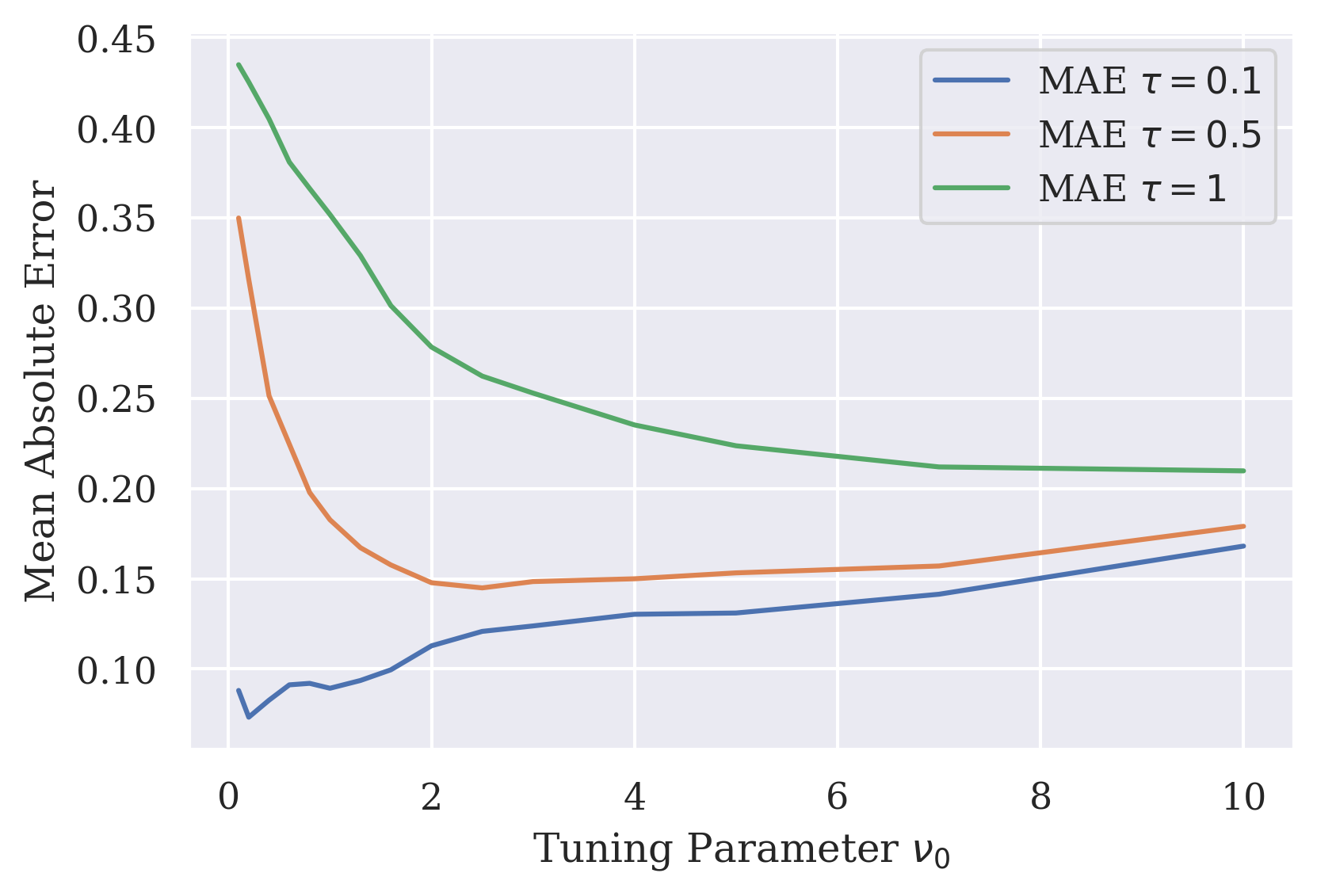
for some tuning parameter . We do not prove that this choice is suitable to our model. However, following Theorem 2 in [7], we can find such that with high probability is a good estimate of . When is small, this means that is small so that the bias induced by (12) is dominating and we still do not get a good convergence rate. Let . Empirically, it appears that this function is increasing and has an inverse continuously Lipschitz on any compact subset of . Therefore in practice, a good estimator of is
where . This expression depends on the tuning parameter , which appears to have only little impact on the resulting estimator , we found no significant difference while testing different values in the interval , see Figure 3. Therefore, we choose in the subsequent tests, which seems to be a good tradeoff. We refer to Figures 4(c) and 5 for detailed results using .


.
| Bias | Std dev | RMSE | NaN | ||
|---|---|---|---|---|---|
| % | |||||
| % | |||||
| % | |||||
| % | |||||
| % | |||||
| % | |||||
| % | |||||
| % | |||||
| % | |||||
| % | |||||
| % | |||||
| % | |||||
| % | |||||
| % | |||||
| % | |||||
| % | |||||
| % | |||||
| % |
.
Remark 5.1.
The implementation in the case with known is similar, though the computation time is much higher. This is due to the presence of the weight function . Indeed, when , we can take and therefore
Using this simplification, the computation time of is of the order . When , other choices of need to be considered, and this simplification does not hold anymore, so that the computation time is of the order , which makes the computation of much slower in practice. Similar problems occur when computing .
Remark 5.2.
When is unknown, an efficient implementation could be obtained using another de-biasing method. Indeed, one could replace the energy levels by
so that (12) gives
In order to use ratios of energy levels, we need to check that does not vanish. This is not trivial and can only easily be checked asymptotically when and since these conditions imply that and we have . The same method can then be applied to build an estimator in that case.
Acknowledgments and fundings
Grégoire Szymanski gratefully acknowledges the financial support of the École Polytechnique chairs Deep Finance and Statistics and Machine Learning and Systematic Methods. Tetsuya Takabatake gratefully acknowledges financial support of JSPS KAKENHI (Grant Numbers JP19K23224 and JP23K13016) and the ANR project “Efficient inference for large and high-frequency data” (ANR-21-CE40-0021). This work was also supported by the Funds for the Development of Human Resources in Science and Technology under MEXT through the Home for Innovative Researchers and Academic Knowledge Users (HIRAKU) consortium. The authors would like to thank Marc Hoffmann and Mathieu Rosenbaum for helpful remarks and discussions.
References
- BF [18] Alexandre Brouste and Masaaki Fukasawa. Local Asymptotic Normality property for fractional Gaussian noise under high-frequency observations. The Annals of Statistics, 46(5):2045 – 2061, 2018.
- BM [18] Alexandre Brouste and Hiroki Masuda. Efficient estimation of stable Lévy process with symmetric jumps. Stat. Inference Stoch. Process., 21(2):289–307, 2018.
- Bru [03] Driver K. Bruce. Analysis Tools with Applications. 2003.
- BSV [20] Alexandre Brouste, Marius Soltane, and Irene Votsi. One-step estimation for the fractional Gaussian noise at high-frequency. ESAIM: Probability and Statistics, 24:827–841, 2020.
- CGLL [13] Serge Cohen, Fabrice Gamboa, Céline Lacaux, and Jean-Michel Loubes. LAN property for some fractional type Brownian motion. ALEA Lat. Am. J. Probab. Math. Stat., 10(1):91–106, 2013.
- [6] Carsten Chong, Marc Hoffmann, Yanghui Liu, Mathieu Rosenbaum, and Grégoire Szymanski. Statistical inference for rough volatility: Central limit theorems. arXiv preprint arXiv:2210.01216, 2022.
- [7] Carsten Chong, Marc Hoffmann, Yanghui Liu, Mathieu Rosenbaum, and Grégoire Szymanski. Statistical inference for rough volatility: Minimax Theory. arXiv preprint arXiv:2210.01214, 2022.
- Coe [01] Jean-François Coeurjolly. Estimating the parameters of a fractional Brownian motion by discrete variations of its sample paths. Statistical Inference for stochastic processes, 4(2):199–227, 2001.
- CR [98] Fabienne Comte and Eric Renault. Long memory in continuous-time stochastic volatility models. Math. Finance, 8(4):291–323, 1998.
- CT [23] Carsten Chong and Viktor Todorov. Asymptotic expansions for high-frequency option data. arXiv preprint arXiv:2304.12450, 2023.
- Dah [89] Rainer Dahlhaus. Efficient parameter estimation for self-similar processes. Ann. Statist., 17(4):1749–1766, 1989.
- Dah [06] Rainer Dahlhaus. Correction: Efficient parameter estimation for self-similar processes. Ann. Statist., 34(2):1045–1047, 2006.
- FT [86] Robert Fox and Murad S. Taqqu. Large-sample properties of parameter estimates for strongly dependent stationary Gaussian time series. The Annals of Statistics, 14(2):517–532, 1986.
- FT [87] Robert Fox and Murad S. Taqqu. Central limit theorems for quadratic forms in random variables having long-range dependence. Probability Theory and Related Fields, 74(2):213–240, 1987.
- GH [07] Arnaud Gloter and Marc Hoffmann. Estimation of the Hurst parameter from discrete noisy data. The Annals of Statistics, 35(5):1947–1974, 2007.
- GJR [18] Jim Gatheral, Thibault Jaisson, and Mathieu Rosenbaum. Volatility is rough. Quantitative finance, 18(6):933–949, 2018.
- Háj [72] Jaroslav Hájek. Local asymptotic minimax and admissibility in estimation. In Theory of Statistics, pages 175–194. University of California Press, 1972.
- IH [81] Ildar A. Ibragimov and Rafail Z. HasMinskii. Statistical estimation: asymptotic theory, volume 16. Springer Science & Business Media, 1981.
- IL [97] Jacques Istas and Gabriel Lang. Quadratic variations and estimation of the local Hölder index of a Gaussian process. Annales de l'Institut Henri Poincare (B) probability and statistics, 33(4):407–436, 1997.
- JLZ [17] Jean Jacod, Yingying Li, and Xinghua Zheng. Statistical properties of microstructure noise. Econometrica, 85(4):1133–1174, 2017.
- JM [15] Jean Jacod and Per A. Mykland. Microstructure noise in the continuous case: Approximate efficiency of the adaptive pre-averaging method. Stochastic Processes and their Applications, 125(8):2910–2936, 2015.
- Kaw [13] Reiichiro Kawai. Fisher information for fractional Brownian motion under high-frequency discrete sampling. Communications in Statistics - Theory and Methods, 42(9):1628–1636, 2013.
- LC [60] Lucien Le Cam. Locally asymptotically normal families of distributions; certain approximations to families of distributions and their use in the theory of estimation and testing hypotheses. Univ. California Publ. Statist., 3:37, 1960.
- LC [72] Lucien Le Cam. Limits of experiments. In Theory of Statistics, pages 245–282. University of California Press, 1972.
- LC [86] Lucien Le Cam. Asymptotic methods in statistical decision theory. Springer, 1986.
- LF [22] Fabien Le Floc’h. Roughness of the implied volatility. arXiv preprint arXiv:2207.04930, 2022.
- LRR [12] Offer Lieberman, Roy Rosemarin, and Judith Rousseau. Asymptotic theory for maximum likelihood estimation of the memory parameter in stationary Gaussian processes. Econometric Theory, 28(2):457–470, 2012.
- Mag [86] Jan R. Magnus. The exact moments of a ratio of quadratic forms in normal variables. Annales d'Economie et de Statistique, pages 95–109, 1986.
- MZ [16] Per A. Mykland and Lan Zhang. Between data cleaning and inference: Pre-averaging and robust estimators of the efficient price. Journal of Econometrics, 194(2):242–262, 2016.
- [30] Peter M. Robinson. Gaussian semiparametric estimation of long range dependence. Ann. Statist., pages 1630–1661, 1995.
- [31] Peter M. Robinson. Log-periodogram regression of time series with long range dependence. Ann. Statist., pages 1048–1072, 1995.
- Ros [08] Mathieu Rosenbaum. Estimation of the volatility persistence in a discretely observed diffusion model. Stochastic Processes and their Applications, 118(8):1434–1462, 2008.
- SSH [14] Till Sabel and Johannes Schmidt-Hieber. Asymptotically efficient estimation of a scale parameter in Gaussian time series and closed-form expressions for the Fisher information. Bernoulli, 20(2):747–774, 2014.
- ST [94] Gennady Samorodnitsky and Murad S. Taqqu. Stable Non-Gaussian Random Processes: Stochastic Models with Infinite Variance: Stochastic Modeling. Chapman & Hall, 1994.
- Swe [80] Trevor J. Sweeting. Uniform asymptotic normality of the maximum likelihood estimator. Ann. Statist., pages 1375–1381, 1980.
- Szy [22] Grégoire Szymanski. Optimal estimation of the rough Hurst parameter in additive noise. arXiv preprint, arXiv:2205.13035, 2022.
- Tak [23] Tetsuya Takabatake. Supplementary article to Corrigendum: Error bounds and asymptotic expansions for Toeplitz product functionals of unbounded spectra''. Journal of Time Series Analysis, forthcoming, 2023.
- VdV [00] Aad W. Van der Vaart. Asymptotic statistics, volume 3. Cambridge university press, 2000.
- Yaj [85] Yoshihiro Yajima. On estimation of long-memory time series models. Australian Journal of Statistics, 27(3):303–320, 1985.
- Yos [11] Nakahiro Yoshida. Polynomial type large deviation inequalities and quasi-likelihood analysis for stochastic differential equations. Annals of the Institute of Statistical Mathematics, 63(3):431–479, 2011.
Appendix A Analysis of the rate matrix
Lemma A.1.
Proof of Lemma A.1.
Before proving Lemma A.1 (3), we start with a few preliminary computations. Fix and let . Recall for and set
| (22) |
where is defined in Assumption 3.3. First note that
so that uniformly on by Assumption 3.3. Since , we have
Multiplying both sides by , and using the inequality , we get
and therefore
uniformly on . Then, using that
we obtain
| (23) |
uniformly on . Moreover, note that we have
for some continuously differentiable function on by Assumption 3.2. Using the fundamental theorem of the calculus, we have
Moreover, (23) gives
| (24) |
and therefore we get
| (25) |
uniformly on .
We are now ready to prove Lemma A.1 (3). First note that we can write
so that using (25), Lemma A.1 (3) follows from
Using the definition of in (22), the triangle inequality and the sub-multiplicative property of the matrix norm , we obtain
| (26) |
Since we have already proved uniformly on , we only need to focus on the terms , and . Computing explicitely , we can show that
and therefore, using Assumption 3.3 and Lemma A.1 (2), we get
| (27) |
Appendix B Proof of Theorem 3.4
B.1. Notation and structure of the proof
We first summarize the notation used in this proof. For , a -matrix and vectors , we write and . For , we write
Then, we define and by
for , and
| (30) |
where . Moreover, we define
| (31) |
Set . For a measurable set of , we write the indicator function of , that is if and otherwise. For with and , we define
Moreover, for fixed, we introduce the following restricted parameter space
For with , and , we write for .
We are now ready to give the structure of the proof. Using the change of the variable and Taylor’s theorem, we can show
where the remainder term is given by
| (32) |
Therefore, the LAN property follows once we have verified (7) and the estimates
| (33) |
and
| (34) |
for each and . Estimates (33) and (34) are proved in Section B.2 and B.3 respectively while (7) follows from (33) proceeding as for the proof of Lemma 2.5 of [5]. These proofs are based on the following result of the trace approximation, which is proved in Section C.
Proposition B.1.
Let and . Suppose that for each , and are periodic functions on with period satisfying
| (35) |
uniformly on compact subsets of for any and each . Then, for each , we define , and , Then we obtain
as uniformly on compact subsets of for any and .
B.2. Proof of (33)
First, note that we have
and
Moreover, we can easily check that
| (36) |
so that we have
Therefore, we obtain the following representation
where
By definition of and and by Assumption 3.3, we get
where
and
Moreover, we have
We need to evaluate these quantities. Using the similar calculations used in the proofs of Propositions B.2 and B.3, which are stated in the end of this proof, and combining them with (36), Propositions B.1, Assumption 3.2 and using that and under Assumption 3.2, we obtain
and therefore
Note that the right-hand side is no longer random, and therefore this implies that (33) is a consequence of
| (37) |
for each . For conciseness, we write
where and are defined in (30) and (31) respectively. Using that
we see that the left-hand side of (37) can be rewritten as
Using that , Proposition B.1 and Assumption 3.2, we also have
as , so that we can show as using as and Lebesgue’s convergence theorem. Note that, since we have , Assumption 3.3 implies
uniformly on for each so that we obtain
Therefore, (37) follows once we have proved the following results:
| (38) |
as for each . Set . First note that, since we have for , we can rewrite
and
Moreover, Proposition B.1 and Assumption 3.2 give
as for each , and
as for each . (38) eventually follows from these two identities and the following propositions, whose proofs are delayed until Appendix D.
Proposition B.2.
Let and . For any , we obtain
Proposition B.3.
Let and . For any , we obtain
B.3. Proof of (34)
We first introduce some notation used in this proof. Let and . Consider functions and satisfying (35) for each . Set and for . For conciseness, we write and . Moreover, for , we write and
| (39) |
For conciseness, we write , .
Recall that is defined in (32). First note that
so that using Chebyshev’s inequality, we know that for any and , is bounded above by
| (40) |
We now use the following Sobolev inequality that can be found in the lecture note by [3], see Corollaries 25.10 and 25.11.
Lemma B.4 (Sobolev Inequality).
Let , be an open subset of and be a sequence of complete probability spaces. Assume that for each , is a continuous stochastic process defined on such that for -a.s. , is a continuously differentiable function on . Then for any satisfying , there exists a constant such that for any , and satisfying ,
hold for -a.s. .
For the first term of (40), Lemma (B.4) and Fubini’s theorem give that for any ,
and
uniformly on . Similarly, for the second term of (40), Lemma (B.4) and Fubini’s theorem also give that for any ,
uniformly on . Therefore (34) follows once we have proved that for any ,
| (44) |
as uniformly on , where is defined in Equation (6). By explicit computation of , and and using Lemma A.1 (1) and the linearity on , we can see that (44) follow once we have proved the following two results:
| (45) |
as uniformly on for any and with , and
| (46) |
for any uniformly on , and , where is defined in (39). On the other hand, expressing moments as sum of cumulants and using the closed form expression for cumulants of Gaussian quadratic forms computed in Lemma 2 of [28] and the homogeneous and translation-invariant properties of cumulants, (45) and (46) follow once we have proved
| (47) |
uniformly on for any , , , and satisfying , and
| (48) |
uniformly on for each and , where we denote for conciseness. Moreover, since we have , (47) and (48) follow from Proposition B.1 once we have proved that
| (49) |
uniformly on for any , , , and satisfying , and
| (50) |
uniformly on for each and . We give the proofs of (49) and (50) in Sections B.3.1 and B.3.2 respectively.
B.3.1. Proof of (49)
We consider separatedly the cases (a) for all and (b) there exists such that .
B.3.2. Proof of (50)
First note that
We start by considering the first integral. We have
and there exists a constant , independent of , , and , such that for any and ,
using (23). Then, we can show that for any and small enough,
uniformly on . Then, for each , we can use (25) and (24) and take small enough to get
| (51) |
Now, we consider the integral . Using that
we can see that there exist constants , independent of , , and , such that for any and ,
Therefore, for any and small enough,
uniformly on . Then for each , we get
| (52) |
Appendix C Proof of Proposition B.1
We prove Proposition B.1 in a similar line with the proof of Equation 5 (a) in the full version of [27].
First note that the mapping on is linear and that we can decompose any function as . Therefore, without loss of generality, we can assume that for each and ,
the function and are non-negative and either or is equal to and the other is positive. Moreover, we assume that the set has a positive Lebesgue measure.
Then we summarize the notation used in the proof of Proposition B.1. Fix satisfying . Write
and for each ,
Since is positive definite for each from the above Assumption , we define
where we write and for conciseness.
Moreover, for , we define
and
Using the triangle inequality, the error is divided into the following two terms:
where
| (53) |
In the rest of the proof, we will derive error bounds of and separately.
C.1. Preliminary result
In this section, we prove the following proposition needed for the proof of Proposition B.1.
Proposition C.1.
Let satisfying . Under the same assumptions in Proposition B.1, we obtain
uniformly on compact subsets of for any and .
C.1.1. Outline of Proof of Proposition C.1
We prove Proposition C.1 proceeding as the proof of Equation 1 of [37]. We first introduce some notation. Fix such that and . We define
| (54) |
where we write for . For each , we write
and where
for , where for .
We also write for conciseness.
Note in addition that
so we obtain the following upper bound for using Lemma 3 of [37]:
uniformly on compact subsets of , where the sums holds over all such that . Therefore Proposition C.1 follows once we have proved the following results.
Lemma C.2.
Suppose the assumptions given in Proposition C.1 to hold. Then the following results hold uniformly on compact subsets of for any .
-
For any and , we have as uniformly on compact subsets of .
-
For any and , we have as uniformly on compact subsets of .
-
For any , we have as uniformly on compact subsets of .
In the rest of this section, we will prove Lemma C.2 (1)-(3) separately.
C.1.2. Proof of Lemma C.2 (1)
For any and each , and , we take for such that for each and ,
and
Note that for each and , we also have
Moreover, since for all , we can show
so that holds for .
Let and be the -periodic function given by on . Define
where and
where we denote by . Using Lemma 2 of [37], we can show that for each , we have
uniformly on compact subsets of and therefore Then we see
uniformly on compact subsets of . Proceeding as the proof of Proposition 6.1 of [14], we can also prove that
uniformly on compact subsets of since the assumption implies . This completes the proof.
C.1.3. Proof of Lemma C.2 (2)
Lemma C.3.
Denote and set , where is defined in (54). For any , we have
| (55) |
uniformly on compact subsets of for any , where we write .
Proof of Lemma C.3.
Fix . We can assume for all without loss of generality. Indeed, implies
| (56) |
where .
Note that Using . Therefore implies for all .
By a straightforward calculation, we can see that the inequality (55) follows once we have proved that for each and and any ,
| (57) | ||||
| (58) |
uniformly on compact subsets of . We firstly verify the inequality (57). By a straightforward calculation, we can show that for any ,
uniformly on compact subsets of .
This completes the proof of (57).
Finally, we verify the inequality (58). First note that can rewriten as
| (59) |
where, for conciseness, we write
Moreover, using the inequality (56), we can also show that
| (60) |
uniformly on compact subsets of . Therefore, using (57), (59) and (60), we can see that (58) follows once we have proved
| (61) |
uniformly on compact subsets of . Note that also implies for any and . Thus, using the inequality (56) and the mean-value theorem, we can show that for each ,
| (62) |
Moreover, we can also show
and
| (63) |
uniformly on compact subsets of . Thus, using the inequalities (56), (57), (62)-(63), we can also show that
| (64) |
uniformly on compact subsets of . Then (61) follows from (62) and (64). ∎
We are now ready to prove Lemma C.2 (2). Since , there exists such that . Then, using Lemma C.3, the definition of in (54) and (56), we can show
| (65) |
uniformly on compact subsets of for any and since is a subset of . The rest of the proof of Lemma C.2 (2) is similar to the proof of Proposition 4 (2) of [37] using the inequality (65) instead of the inequality (5) of [37]. We omit the details for conciseness.
C.1.4. Proof of Lemma C.2 (3)
C.2. Proof of Proposition B.1
Using Proposition C.1, it suffices to prove that
| (66) |
uniformly on compact subsets of for any , where is defined in (53). By definition of and , we have
and therefore
where we write
and where and for conciseness. In the rest of this proof, we evaluate the four terms , , and as for each separately.
Estimate of : First note that
| (67) |
Moreover, using that and the properties of Frobenius and operator norms, we have
Therefore, we obtain
| (68) |
uniformly on compact subsets of for any and using the two following lemmas.
Lemma C.4.
Let satisfying . Under the same assumptions in Proposition B.1, we obtain
uniformly on compact subsets of for any .
Proof of Lemma C.4.
Lemma C.5.
Under the same assumptions in Proposition B.1, we obtain
as uniformly on compact subsets of for any , and .
Proof of Lemma C.5.
Estimate of : Using (67), that , the properties of Frobenius and operator norms, and the Cauchy-Schwarz inequality, we can show
Therefore, we obtain
| (69) |
uniformly on compact subsets of for any and using Lemmas C.4, C.5 and the following lemma.
Lemma C.6.
Let . For any satisfying and , we obtain
| (70) |
uniformly on compact subsets of .
Proof of Lemma C.6.
First note that we can write
so that Lemmas C.4 and C.5 provide that for any and ,
uniformly on compact subsets of as . Then we conclude (70) in the case . In the rest of this proof, we will prove (70) in the case by mathematical induction. In the following, we assume that for all satisfying and , it holds
| (71) |
uniformly on compact subsets of . Using the same decomposition used in the equation (13) of [11] and elementary properties of the Frobenius norm and the operator norm, we can show
| (72) |
Therefore, we conclude (70) in the case from Lemma C.5, the Assumption (71) of the mathematical induction, Equation (72) and
This completes the proof. ∎
Estimate of : First note that
Therefore, using Proposition C.1, we obtain
| (73) |
uniformly on compact subsets of for any , and .
Estimate of : Using the Cauchy-Schwarz inequality, we can show
| (74) |
Moreover, we can also prove
| (75) |
uniformly on compact subsets of for any , and using Proposition C.1 proceeding as the proof of the term . Therefore, using (74), (75) and Lemma C.6, we can show
| (76) |
uniformly on compact subsets of for any , and .
Appendix D Proofs of Propositions B.2 and B.3
D.1. Proof of Proposition B.2
We first introduce some notation used in this Section. For sequences of functions and on which are not equal to zero on , write as uniformly on if
For , we write , and
Note that , and as uniformly on .
Before proving Proposition B.2, we prepare the following three lemmas.
Lemma D.1.
Let and be a positive sequence satisfying
uniformly on . Under the same assumptions in Proposition B.2, we obtain
uniformly on .
Proof of Lemma D.1.
Set . First note that by defintion of , we have and as uniformly on since . Therefore, and
uniformly on . Since we have uniformly on , we obtain
uniformly on . Then the conclusion follows from the assumption of using that so that
This completes the proof. ∎
Lemma D.2.
Let and be a positive sequence satisfying
| and as |
uniformly on . Under the same assumptions in Proposition B.2, we obtain
uniformly on .
Proof of Lemma D.2.
Recall that . Using the change of variable , we obtain
Moreover, we can see from the definition of , see (31) that and therefore
Then, using the convergence as , we get
uniformly on , which concludes the proof. ∎
Lemma D.3.
Let and be a positive sequence satisfying
| (77) |
uniformly on . Under the same assumptions in Proposition B.2, we obtain
uniformly on .
Proof of Lemma D.3.
Recall that , and . For , we also set
and for , we write
and
Note that
From the definitions of , , and , we can show
| (78) |
and
uniformly on . Proceeding as the proof of Lemma D.2, we also have
uniformly on . Using the definitions of and and Taylor’s theorem, we have
| (79) | ||||
uniformly on . Moreover, Taylor’s theorem also yields
uniformly on . On the other hand, we can show and
Thus we conclude (79) from the above calculations. Then, using the inequalities (78)-(79), we also conclude
uniformly on . This completes the proof. ∎
D.2. Proof of Proposition B.3
Since and , we have
uniformly on . Moreover, since we have and from Assumption 3.3, we obtain
as uniformly on . This completes the proof.
Appendix E Explicit Expressions of
In this section, we derive explicit expressions of for when with . For conciseness, we write
By definition, we have
and
for . Moreover
and
so we obtain
Similarly, we have
and
Appendix F Proof of the results of Section 4.1
F.1. Proof of Lemma 4.2
First, note that by self-similarity and the fact that has stationary increments, we have
It follows that is well defined for all values of and . Moreover, a direct computation of the expectation above yields
where .
We now focus on the decay of the autocorrelation function. By symmetry, it suffices to show this decay only for . Since is self-similar and has stationary increments, we can compute explicitly this autocorrelation function and we have
| (80) |
where . For , the absolute values appearing in the expression of can be removed and we can use Taylor’s formula to expand around . Let , we have
Then we infer for some constant and independent of . Summing over and in (80) yields the result.
F.2. Proof of Lemma 4.3
It is cleat from its definition that is differentiable in and therefore is differentiable. Using usual theorems for derivation under the integral, we also know that is differentiable.
Moreover, since is Lipschitz continuous (since it is differentiable with bounded derivative on ) and for any , we deduce that
We show similarly the bound .
It remains to prove the uniform control on and on . Recall from Lemma 4.2 that . Moreover, whenever there exists such that . This is the case whenever by Assumption 4.1. Using also continuity of for any fixed , we know that for all and that for all . To get the uniformity in of (10), we use the uniform convergence (by Lemma 4.3), the fact that and that
F.3. Proof of Lemma 4.4
Under Assumption 2.1, we have in distribution for some standard Gaussian variables
| (81) |
in distribution, where
| (82) |
Since the are independent standard Gaussian variables, we can compute the variance of from (81) and in particular, is well defined. The precise computation of require delicate handling because of the crossovers between for and for close to . Indeed, we obtain
From (82), the coefficients are bounded uniformly so that the sequence is bounded.
Suppose now that Assumption 4.1 holds. Note that since the first derivatives of vanish at and at , we have whenever of . For , we have by Taylor-Lagrange’s formula
for some . Using also that whenever , we get
| (83) |
Using finally that is continuous, we retrieve the same bound for . Combining this with the explicit expression for obtained previously yields the upper bound on in Lemma 4.4.
F.4. Proof of Proposition 4.5
Recall that . Therefore, using Lemmas 4.2 and 4.4 and the independence between and the noise , we obtain
Then, using Wick’s theorem and the independence between and again, we obtain
We first derive the upper bound. Using Lemma 4.4, we know whenever and we obtain
uniformly on whenever . Together with Lemma 4.2, we obtain
uniformly on and we conclude since .
Appendix G Proof of the results of Section 4.2
G.1. Proof of Lemma 4.6
Recall that and that is defined in (16) by
Since and is invertible on with inverse uniformly Lipschitz on the compact sets of , it suffices to prove that
is bounded in -probability, uniformly over . We first prove a lower bound (in -probability) for .
Lemma G.1.
There exists such that
Proof.
Now we return to the proof of Proposition 4.5. Consider as in Lemma G.1. Then we can show that for any ,
as uniformly on compact subsets of . Moreover, a straightforward calculation gives
where
Therefore, the conclusion follows once we have proved that , and are bounded in -probability, uniformly over .
G.2. Proof of Lemma 4.7
Since and is invertible on with inverse uniformly Lipschitz on the compact sets of , it suffices to prove that
is bounded in -probability, uniformly over . Moreover, since , it suffices to prove that
| (85) |
is bounded in -probability, uniformly over . Note that, for each , the random variable in the sequence (85) is bounded above by , where
Therefore, the conclusion follows once we have proved that both and are bounded in -probability, uniformly over .
We start with the variance terms . By Proposition 4.5, we have
uniformly on and therefore is bounded uniformly which ensure tightness of .
For the bias terms , we use Proposition 4.5 to get
which is bounded in -probability, uniformly over since for each .
G.3. Proof of Proposition 4.9
Since and is invertible on with inverse uniformly Lipschitz on the compact sets of , it suffices to prove that
is bounded in -probability, uniformly over . Moreover, Using Lemma 4.8 and the assumption on , it suffices to show that for each , the sequence
is bounded in -probability, uniformly over . Furthermore, since we know that uniformly on Using Lemma 4.3 and as uniformly on by the definition of , it suffices to prove that
| (86) |
is bounded in -probability, uniformly over . Recall then from Proposition 4.5 that
so that for each , the random variable in the sequence (86) is bounded above by
where
Therefore, the proof is down to proving that each sequence of these five terms is bounded in -probability, uniformly over .
Uniform boundedness of . Note first that
Therefore, using that is bounded in -probability, uniformly over and that we have as uniformly on , we obtain that is uniformly bounded.
Uniform boundedness of . Note that it suffices to prove that is bounded uniformly over . By Proposition 4.5, we have
uniformly on . Then, by the definitions of and , we have
uniformly on and the conclusion follows because by definition of .
Uniform boundedness of . We use again the definition of and together with Lemma 4.4 ensuring that uniformly on to show that
Then the conclusion follows because is bounded in -probability, uniformly over from the assumption on .
Uniform boundedness of . By the definitions of , and , Taylor formula and Lemma 4.3, we have
uniformly on . Then the conclusion follows from the assumption on .
Uniform boundedness of . Note that is bounded uniformly on by the definition of . Moreover, is bounded by Lemma 4.3. Therefore, it suffices to prove that is tight uniformly over . But recall from Taylor’s formula that for any real , we have . Thus
and we conclude the proof using that is bounded, that is uniformly tight by applying the same ideas as for and that is uniformly tight.
G.4. Proof of Proposition 4.10
Since and is invertible on with inverse uniformly Lipschitz on the compact sets of , it suffices to prove that
is bounded in -probability, uniformly over . Moreover, Using Lemma 4.8 and the assumption on , it suffices to prove that for each , the sequence
is bounded in -probability, uniformly over , where we write . We start by proving a result similar to Lemma G.1.
Lemma G.2.
There exists such that
uniformly on .
Proof.
Proceeding as in the proof of Lemma G.1, but using
instead of (84), we can show that for small enough,
uniforly on . Moreover, we know from (15) that is given by
Proceeding as for in the proof of Proposition 4.9, we also see that is bounded in -probability, uniformly over and therefore the proof of Lemma G.2 is down to proving that, uniformly over , we have
| (87) |
We start with the first limit. Since and by assumption and using also that uniformly on by construction and Lemma 4.3 to bound the difference , we obtain
uniformly on , which proves is bounded in -probability uniformly over .
We now return to the proof of Proposition 4.10. Consider as in Lemma G.2. Then we can show that for any ,
as uniformly on and it is therefore enough to prove that
is uniformly bounded in probability. But by its definition, it is bounded by above by , where, for , we have
Thus, the proof is down to proving that each sequence of these terms is bounded in -probability, uniformly over . We omit the proofs of and as they are similar to the proofs of and in Proposition 4.9 respectively. Instead we focus on the sequence with and ¡e consider only in the case of since the result can be proved similarly for . By definition of and using and results similar to the uniform stochastic boundedness of and in the proof of Proposition 4.9, we can show
uniformly on , where
Since Lemma 4.3 gives for uniformly on , we obtain
uniformly on . Then note that we have
and the RHS of the above inequality converges to in -probability (uniformly over ) as since is bounded in -probability and as uniformly on . Then, the conclusion follows since and the sequences and are bounded in -probability, uniformly over .
G.5. Proof of Proposition 4.11
Proceeding as in the proof of Lemma 4.7, it suffices to prove that
is bounded in -probability, uniformly over . For each , the random variable in the above sequence is bounded above by , where
Since we see that is bounded in -probability, uniformly over proceeding as for in the proof of Lemma 4.7, it suffices to prove that is bounded in -probability, uniformly over . Using Lemma 4.3, we know that is bounded and differentiable with bounded derivative on . Therefore, the absolute value of the derivative of the function is bounded by for some uniform constant . Since we also have and , we can show
uniformly on . Then we finish the proof since and the sequences and are bounded in -probability, uniformly over .
G.6. Proof of Theorem 4.12
Recall that . We define
and by induction
for each . Then Lemmas 4.6 and 4.7 and Proposition 4.9 ensure that
| , and |
are bounded in -probability, uniformly over . Moreover, Propositions 4.10 and 4.11 yield that for each ,
| , and |
are also bounded in -probability, uniformly over .
Since implies for each , we conclude by induction that
Then the conclusion follows because holds for any from the definition of so that we obtain and due to .
Appendix H Proof of Theorem 4.14 and Lemma 4.15
H.1. Proof of Theorem 4.14
Using Lemma A.1, we can assume without loss of generality that is invertible on . For conciseness, we write , and
First note that we have
Using Taylor’s theorem, we have
Then, we obtain
| (88) | ||||
Using (21) and the continuity of on , we know that in distribtion as and using also Lemma A.1, in distribtion as . Moreover, proceeding as the proof of (34), we can show
for each , so that (21) gives
We conclude by plugging the last limit, and , and (7), into (88) (using Slutsky’s lemma).
H.2. Proof of Lemma 4.15
Write . Using the notation of Section A, we have
Since we have and uniformly on , the conclusion follows.
