BGLS: A Python Package for the Gate-by-Gate Sampling Algorithm to Simulate Quantum Circuits

The gate-by-gate sampling algorithm can be easily modified if some operations in $U=U_{d}\dots U_{1}$ are non-unitary. BGLS supports this case as long as the apply_op function provided to the bgls.Simulator can decompose operations - this task is particularly easy in Cirq and an example is discussed in the documentation at https://asciineuron.github.io/bgls/features.html. In this case the method of quantum trajectories is applied to simulate non-unitary operations. Two common use cases of non-unitary operations are noisy simulation and mid-circuit measurement and these are fully supported in BGLS. The only difference relative to unitary circuits is that automatic sample parallelization (Sec. 3.2.3) typically cannot be applied in quantum trajectories since the number of wavefunctions is much larger than the number of samples.

BGLS provides support to optimize circuits for the gate-by-gate sampling algorithm through the function bgls.optimize_for_bgls. As a simple but illustrative example, consider a circuit with five sequential single-qubit operations. The circuit optimization will merge these operations into one single-qubit operation so that the bitstring only gets updated once instead of five times. An example is provided in the BGLS documentation at asciineuron.github.io/bgls/tips.html. As shown there, circuit optimization on random eight qubit circuits with up to 50 layers of operations leads to a runtime improvement between 1.5x and 2x.

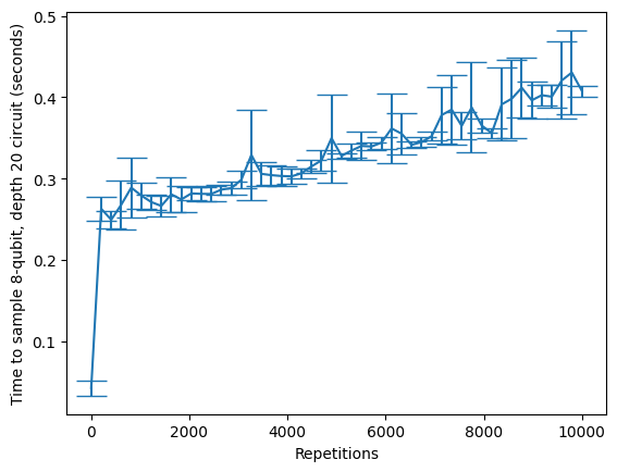
While the gate-by-gate sampling algorithm as presented in Sec. 2 updates one bitstring per evolution of $\Psi$, all bitstrings can be updated in parallel when $\Psi$ is the same for all bitstrings. The basic idea is that for generating N samples, a list of N bitstrings is created, and at every step all are independently updated as expected. To further improve performance, bgls represents this as a dictionary mapping each current unique bitstring b to its multiplicity m. At each gate we then determine all candidates for every b and draw m updated samples. Sampling performance can be seen in Fig. 2. In particular, runtime saturates at large repetitions as there are at most $2^{n}$ unique bitstrings for an $n$ qubit system, limiting the total dictionary size.

For circuits with non-unitary operations, the final state is stochastic and must be rerun for each sample desired. Additionally as shall be described below, sampling near-Clifford circuits using act_on_near_clifford must be repeated to fully explore the space.

BGLS only directly supports Cirq circuits, but most circuit classes from quantum software packages can convert to and from Cirq circuits. For example one can convert a QASM circuit (Cross et al., 2017) via from cirq.contrib.qasm_import (Developers, [n. d.]). An example is shown at asciineuron.github.io/bgls/features.html

We first briefly review some core concepts necessary to understanding Clifford circuits and stabilizer states. This is by no means comprehensive and many sources can be found elsewhere.

First is the definition of the Pauli group. For a system of $n$-qubits, the Pauli group $G_{n}$ is a matrix group consisting of all possible applications of I and the Pauli matrices X, Y, and Z, along with prefactors $\pm 1$, $\pm i$ to each of the qubits’ Hilbert spaces in the tensor product. As an example, for 1 qubit this set consists of $\{\pm I,\pm iI,\pm X,\pm iX,\pm Y,\pm iY,\pm Z,\pm iZ\}$.

Given this, an $n$-qubit stabilizer state $|\Psi\rangle$ is any state such that there exists a subgroup $S\leq G_{n}$ of size $2^{n}$ that stabilizes the state, that is for every $s\in S$, $s|\Psi\rangle=|\Psi\rangle$. For example, if $|\Psi\rangle=1/\sqrt{2}(|0\rangle+|1\rangle)$, we see it is stabilized exactly by I and X. In particular, an additional consequence is that stabilizer states are exactly those which are reachable from $|0^{n}\rangle$ by applying exclusively the so-called Clifford gates. These consist of I, H, S, CNOT, and any combination thereof (e.g. they thus include the Pauli gates from combinations of S and H).

A final important reminder is that these states fall under the Gottesmann-Knill theorem (Gottesman, 1998). This states that any circuit consisting only of initial basis state preparation, Clifford gate applications, and measurement of the qubits in the computational basis is able to be efficiently simulated classically.

To be able to work with such circuits, the first ingredient our bgls sampler needs is a concrete representation of the state. For this, we turn to the so-called ”CH-form” representation (Bravyi et al., 2019), which is itself an extension of the “stabilizer tableaux” (Aaronson and Gottesman, 2004). An existing implementation of this can be found via cirq.sim.StabilizerChFormSimulationState, which bgls
builds upon to provide necessary tooling. We give a brief recap of the structure of this representation and how bitstring amplitudes can be computed.

The original paper showed that in general, any stabilizer state can be expressed as $|\Psi\rangle=\omega U_{C}U_{H}|s\rangle$, where $U_{c}$ is a tensor product of some number of S and CNOT gates, and $U_{H}$ is a product of H and I gates. $\omega$ is a complex scalar, and $|s\rangle\in\{0,1\}^{n}$ (Bravyi et al., 2019).

The state of the system was specified with $n\times n$ binary matrices F, G, M, a phase $\gamma\in\mathbf{Z}_{4}^{n}$, and $v\in\{0,1\}^{n}$. The equations relating these to $U_{C},U_{H}$ are:

Cirq’s implementation directly stores these variables, and wraps handling of gate application with the native act_on protocol. Lastly, we need to be able to compute the probability of an arbitrary bitstring $P(b)$ for such a state. The corresponding bitstring amplitude was given, up to some $\mu\in\mathbf{Z_{4}}$ as:

This is found in StabilizerChFormSimulationState’s
inner_product_of_state_and_x function, from which computation of the probability is trivial. Of note is the computational complexity for this class of states. The cost of computing a desired probability was originally derived (Bravyi et al., 2019) to be $O(n^{2})$ for $n$ qubits, which is polynomial rather than exponential, and notably independent of the circuit depth. From this we can see that $f(n,d)=O(dn^{2})$.

Given the above framework, we turn to our implementation and support of this in bgls. Specifically, the package provides the compute_probability_stabilizer_state function. This operates on any valid
StabilizerChFormSimulationState and calculates via the above the measurement probability of a desired bitstring.

We are able to investigate the runtime scaling of sampling from such a state by constructing random circuits with the bgls
generate_random_circuit function. This is derived from the Cirq equivalent, but provides simpler specification of the target gate set. We construct random circuits consisting exclusively of H, S, and CNOT gates, and either vary the depth of the circuit or the number of qubits in the system. Observed in Fig. 3 is characteristic runtime scaling, confirming expected behavior.

It can be seen that the gate-by-gate sampling algorithm for these states is of an equivalent computational complexity as traditional sampling, and offers no direct benefit. However, the framework for handling these stabilizer states allows sampling from much more promising near-Clifford circuits as we discuss in the following section.

Importantly, pure Clifford circuits and stabilizer states are inherently limited as the Clifford gate set is not universal. That is, it is not necessarily possible to approximate an arbitrary circuit solely in terms of these gates. Commonly used to remedy this is the Toffoli gate, which together with the Clifford group forms a universal gate set (Kliuchnikov, 2013). This no longer satisfies the Gottesman-Knill theorem, hence such circuits are not necessarily efficiently simulable. However, in many cases only relatively few T gates are needed to express a circuit. This allows leveraging the stabilizer state framework on a much larger class of circuits, and forms the basis of the sum-over-Cliffords technique presented in the same paper as the CH-representation (Bravyi et al., 2019). We first briefly recap their results, and then show its implementation in bgls.

Their idea is that any non-Clifford gate $U$ can be decomposed into a sum of Clifford gates $K$ as $U=\sum_{i}c_{i}K_{i}$. This was quantified by the “stabilizer extent” $\zeta$ which is the minimum norm of all such possible decompositions, and gives a heuristic of how non-Clifford the system is.

In particular it was shown that any diagonal rotation gate $R(\theta)=e^{-iZ\theta/2}$ is ideally decomposed as

where $S$ is the Phase gate $S=T^{2}$. Notably, T can be equivalently written as $R(\pi/4)$ and hence expanded in this way.

Taking advantage of this, we implement it in bgls with the novel function act_on_near_clifford for gate application, which enables sampling from general Clifford+$R_{Z}(\theta)$ circuits by simulating with a stabilizer state. This functionality is new to Cirq, where the stabilizer state simulator is limited to pure Clifford circuits.

Its method of operation is straightforward: for any gate with a stabilizer effect checked via cirq.has_stabilizer_effect, the standard act_on is applied. For a $R_{Z}(\theta)$ gate (a subclass of
cirq.ops.common_gates.ZPowGate), we extract $\theta$, compute the relative probabilities of I and S by the above equation, and choose one following this distribution to substitute for $R$.

For a circuit with $N$ such $R(\theta)$ gates, there are clearly $2^{N}$ terms in the final expansion. Hence, for a given sample we are stochastically exploring only one of these branches. In the following section we investigate the results of using stabilizer states on such near-Clifford circuits.

What follows can similarly be found with implementation details on the project’s homepage. As a first analysis, we compare the accuracy of simulating near-Clifford and pure-Clifford circuits. A random circuit is constructed consisting of Clifford+T gates, and a copy is made where each T gate is substituted by S. We sample from these using both the bgls stabilizer state simulator, as well as an exact cirq.Simulator, and plot in Fig. 4 the fractional overlap with what we would expect from the ideal distribution. Observed is a noticeable lag for bgls applied to non-Clifford circuits, i.e. using the sum-over-Cliffords technique. This arises from the $2^{\#T}$ stabilizer states required to represent the non-Clifford circuit, and hence a given number of samples will explore a correspondingly smaller portion of the output distribution.

Next, we explore the effect rotation angle has on output fidelity. We take a fixed random Clifford+T circuit and varying $\theta$, substitute all T with $R(\theta)$. Again the overlap with the ideal distribution is plotted for a fixed number of samples, both for an exact simulator and our sum-over-Cliffords implementation. We see in Fig. 4 an overlap for bgls that greatly fluctuates with angle used. This suggests that perhaps $R(\theta)$ near maxima of this plot could provide a more efficient alternative to T gates in achieving a universal gate set, and could be an avenue for future investigation.

As a last comment about such near-Clifford simulation techniques, we alternatively examine the effect of T gates by instead constructing a random pure-Clifford circuit of 100 moments and progressively replace more gates with T. For each circuit we plot overlap for a fixed number of samples. As the circuit becomes increasingly non-Clifford, we observe in Fig. 5 a decrease in overlap. This highlights the namesake of near-Clifford, in that adequate performance is limited by the degree in which the circuit is non-Clifford.

Perhaps the most promising state representations to use with bgls are those based on matrix product states (MPS), and we provide full support and examples for working with these. Such states have been of great interest to researchers in recent years, and there is much relevant literature for readers interested in more comprehensive information (Perez-Garcia et al., 2007; Biamonte and Bergholm, 2017). Here, we focus our attention on the specific MPS form presented in the paper “What limits the simulation of quantum computers?” (Zhou et al., 2020).

In their notation, any $n$-qubit state can be written in the tensor network form:

Each $i_{j}\in\{0,1\}$ and hence we can see that this is a sum of tensor product terms over possible computational basis (i.e. bitstring) states. There is a unique tensor $M(j)$ corresponding to each qubit. For each of these, the tensor dimensions are given by $i_{j}$ of size 2, corresponding to the given qubit’s 0 and 1 components, and $\mu_{j}\in\{1,\dots,\chi_{j}\}$ of size $\chi_{j}$. $\chi$ is referred to as the local dimension, and is a quantity that increases with and controls the degree of entanglement with other qubits.

It is thus evident that retrieving any quantity of interest (here again bitstring amplitudes) necessitates expensive contraction of this tensor network. As we saw, $\chi$ dominates the size of these tensors, and thus matrix product states are most useful where the total degree of entanglement is limited.

Handily, this structure is already implemented to interface with Cirq via the experimental
cirq.contrib.quimb.MPSState class. We next examine the data structures and show how specific bitstring amplitudes can be computed, a feature not present in the existing implementation.

In particular, a MPSState stores a list of $n$ quimb (Gray, 2018) tensors M representing the above. Upon investigation, we see each is initially of shape $(2,)$ (this corresponds to the $i_{j}$ dimension), and for each additional qubit it is entangled with by multi-qubit gates, it gains another axis of dimension 2. An MPSState is able to compute the full state vector by completely contracting this tensor network.

bgls improves upon this by allowing calculation of specific bitstring amplitudes, a feature not natively provided by the MPSState class. By considering only a single bitstring, at each qubit we can eliminate the first tensor axis, choosing the index matching the desired bitstring’s value. This tensor subset is extracted with the quimb isel function, where the appropriate tensor label is provided with the MPSState’s i_str function. Proceeding this way through all $n$ tensors, a subnetwork is created of much smaller size. The desired amplitude is then the result of full contraction of this reduced network, and is much less computationally intensive. This algorithm and the necessary quimb functions can be understood as follows:

def mps_bitstring_probability(mps, btstr):    M_sub = []    for i, Ai in enumerate(mps.M):        qindx = mps.i_str(i)        A_sub = Ai.isel({qindx: int(btstr[i])})        M_sub.append(A_sub)    tn = qtn.TensorNetwork(M_subset)    st = tn.contract(inplace=False)    return np.power(np.abs(st), 2)

A more complete walkthrough with graphical representation can be found in bgls’s documentation (Shapiro and LaRose, 2023).

Armed with a state representation and bitstring probability function, we are now ready to use bgls with MPS for circuit sampling. As a naive example, we consider a GHZ circuit with randomly sequenced CNOTs (Gray, 2018). Importantly, GHZ states can be analytically represented trivially with MPS due to their symmetries. However, when blindly simulating these circuits this example becomes particularly hard as GHZ states are maximally entangled.

Quantifying this, we construct such random GHZ circuits of width 2-20 and perform sampling with both the MPS and state vector representations. A characteristic circuit and a plot of the runtimes is seen in Fig. 6. Observed is exponential runtime scaling of both representations. This demonstrates MPS’s exponential scaling with entanglement, and emphasizes that one needs particular care to achieve full performance from tensor network states.

Repeating the same procedure but instead with a random circuit of fixed depth at each width, we see in Fig. 7 that using a MPS representation has drastically reduced runtime compared to a state vector. In this case, only a subset of gates are multi-qubit and entanglement producing. Hence for a shallow enough circuit the degree of entanglement lags behind the maximum (which exponentially increases with width). We could expect that for deep enough random circuits of a given width, all qubits are eventually entangled and MPS performance gains would give way.

Lastly, we consider random circuits of increasing width consisting of 1-qubit gates and a fixed number of 2-qubit CNOT gates. We observe in Fig. 7 a near linear sampling runtime scaling. Taken together, these results corroborate the $O(n\chi^{3})$ computational complexity of calculating amplitudes as was originally estimated (Zhou et al., 2020).