Observation of a Topological Phase Transition in Random Coaxial Cable Structures with Chiral Symmetry
Abstract
We report an experimental study of the disordered Su-Schrieffer-Heeger (SSH) model, implemented in a system of coaxial cables, whose radio frequency properties map on to the SSH Hamiltonian. By measuring multiple chains with random hopping terms, we demonstrate the presence of a topologically protected state, with frequency variation of less than 0.2% over the ensemble. Connecting the ends of the chains to form loops, we observe a topological phase transition, characterised by the closure of the band gap and the appearance of states which are delocalised, despite the strong disorder.
The Su-Schrieffer-Heeger (SSH) modelSSH , originally a description of the electronic states in polyacetylene, is one of the simplest systems of topological physics. It consists of a chain of sites, representing carbon atoms, connected by hopping terms which alternate in strength, corresponding to the bonds of the dimerised molecule. In this periodic form, it has a band gap which closes when the two hopping strengths are the same. The gap closure separates two topological phases, determined by the relative magnitudes of the hopping amplitudes. With appropriate termination, SSH chains can support localised boundary states which are said to be topologically protected, because their energy is independent of disorder in the hopping amplitudes. These non-trivial topological properties are a consequence of the chiral, or sublattice, symmetry of the SSH model: the sites can be divided into two sublattices, such that there are only hopping terms connecting the two types.
The topology of the SSH model is robust in the presence of disorder, provided that the chiral symmetry is not broken. A chain with a random sequence of hopping amplitudes can still be assigned to one of two topological phases. We can thus talk about a topological phase transition in an ensemble of random SSH loops, driven by varying the parameters in the probability distribution from which the hopping amplitudes are drawnrandom-mondragon-shem . The theory of such random chains, with off-diagonal disorder, has a long history, dating back to work by Dysondyson ; dyson-theodorou ; dyson-eggarter and continuing through modern scaling theories of the Anderson transitiondos-mckenzie ; supersymmetry-balents ; scaling-brouwer ; fokker-titov ; anderson-evers . If the probability distribution for each hopping term is the same, leading to structures which are close to the topological phase boundary, the states at zero energy are predicted to be delocalised. Determination of the localisation properties can thus provide a signature of a topological phase transition. In an infinite chain, the transition is also predicted to be accompanied by a singularity in the density of states.
There have been numerous experimental studies of implementations of the SSH model using electromagnetic waves, in photonic and microwave structuresphotonic-ozawa ; photonic-malkova ; microwave-poli ; polariton-st-jean ; plasmon-bleckmann , and discrete electronicselectrical-ningyuan ; electrical-lee . It is generally hard to control all the couplings in these systems so as to maintain chiral symmetry sufficiently to observe the effects we discuss, particularly while introducing controlled disorder. This is more easily done in cold-atom systemsatom-atala , where delocalisation at a topological phase boundary has been observedatom-meier for a momentum-space SSH structure.
Coaxial cable networks are a very simple electromagnetic system which can be used to investigate disorderlocalisation-zhang and topologicalangular-momentum-jiang ; non-abelian-guo physics. We have shownwhittaker that cable structure can be fabricated with radio frequency properties which map very accurately onto the SSH Hamiltonian. The hopping amplitudes are determined by the impedances of the corresponding cables, so it is easy to make a random ensemble of chains with full chiral symmetry. In this letter, we use cable structures to investigate experimentally the properties of random SSH chains. By the use of impedance and transmission measurements, we demonstrate very precise topological protection of a state, and show the delocalisation and closing of the gap at the phase transition.
The derivation of the matrix description of a coaxial cable network is given in the Supplementary Materials, S1. We consider a network consisting of a set of sites, labelled , connected by sections of coaxial cable, all of which have the same transmission time, , the length divided by the transmission speed. The cable connecting sites and has electrical impedance . The network has radio frequency resonances which are determined by a matrix eigenvalue equation , where the dimensionless ‘energy’, , is related to the frequency, , by . The components of the vector are the voltages at the sites, scaled such that the actual voltage is . Here , with the sum taken over the sites directly connected to . The matrix elements of the ‘Hamiltonian’ are then the hopping amplitudes
| (1) |
This one-to-one mapping from cables connecting sites to hopping amplitudes means it is possible to create a network corresponding to any finite real matrix Hamiltonian, though in practice this is limited by the availability of cables with arbitrary impedances.
We measure the radio frequency properties of the cable structures using a vector network analyser (VNA). Two sorts of measurement are useful. A single port reflection measurement of the parameter gives us the impedance of the structure measured at a given site. We show, in Supplementary Materials S2, that the real part of this is proportional to the local density of states, broadened only by losses in the cables. This enables us accurately to determine the frequencies of the resonances of the structure. Two port transmission measurements () provide information about the spatial extent of the states, allowing us to detect the delocalisation which occurs around the phase transition.

A Hamiltonian has chiral symmetry if the sites can be divided into two sublattices, which we call ‘black’ and ‘white’, Fig.1, such that there is only hopping between sites on different sublattices. There can be no intra-sublattice terms, including on-site energies. If this is the case, ordering the basis such that all the black sites proceed the white sites gives an anti-diagonal form:
| (2) |
From this we obtain , so the eigenvalues must either be zero, or occur in symmetric pairs with opposite signs. It immediately follows that for a chain with an odd number of sites there must be at least one zero energy state. Since this conclusion does not depend on the values of the hopping amplitudes which form the matrix elements of , the zero-energy state is topologically protected against disorder. More generally, for a chiral network with black sites and white sites, there are at least protected states.

Fig.2 shows the local density of states measurement for a number of structures consisting of sequences of 16 cables connected end-to-end. The individual cables are randomly selected from two impedances: and . The structures thus map onto finite length SSH chains with randomised hopping terms. More details of the cables are given in the Supplementary Materials S3. Fig.2(a) shows unlooped chains, with the measurement on a site at the end of the structure. The 16 cables correspond to 17 lattice sites, so we see, as expected, a topologically protected state, at a frequency of approximately 114MHz. The topological protection is very good: the inset shows combined results for this state in 41 random structures. The standard deviation of the resonance energy is approximately 0.22MHz, which we believe is due to small errors in the lengths of the cables.
A topological phase transition is signalled by the presence of a pair of degenerate states at zero energy, equivalent to the gap-closure in a periodic structure. When , this corresponds to the condition that the determinant tps-comment . For our structures, is just the product of the hopping amplitudes, which cannot be made zero without cutting the chain, so there is, trivially, only one topological phase. However, by joining the ends of the chains to form loops, we can observe a transition between the two phases of the SSH model, using measurements of the local density of states. For chiral symmetry, the loops must consist of an even number of sites, and thus be made from an even number of cables. In a loop with cables, labelling hopping amplitudes rather than the sites, (Fig.1), we obtain
| (3) |
However, since the contain the scaling factors as well as the cable impedances , Eq.(1), it is convenient to look at the quotient of the two terms, where these cancel, and define a quantity
| (4) |
For our structures, where the impedances are taken from a binary distribution, or , there are typically cancellations in the ratio of the impedances, and we can write
| (5) |
where is an even integer, which we call the ‘reduced length’ of the structure. For a loop where the length is an even multiple of 2, , when is zero. The sign of is thus a topological invariant; if the hopping terms were changed continuously, it would not be possible to flip the sign of without passing through a marginal structure with . For odd multiples of 2, , the two terms in the expansion of have the same sign, so, though can be zero, to make a topologically marginal structure would require a negative hopping amplitude in the loop.
If, instead of making a loop, the chain is infinitely repeated to form a periodic structure, we find that the topological classification from the sign of the reduced length always agrees the generalised Berry phaseberry-marzari and winding number invariants obtained from Brillouin zone based calculations. These methods also predict a phase transition when in a chain with an odd number of pairs. In a periodic structure this is correct, because there are gap closures somewhere in the Brillouin zone for both even and odd numbers of pairs. The two cases differ because, for an even number of pairs, the closure is at wavenumber where the state is the same at the end of each period, corresponding to the boundary condition for a loop. For an odd number of pairs, the closure is at , so the loop boundary condition is not satisfied. However, as we show below, the delocalisation associated with the phase transition can be seen for both even and odd numbers of pairs. The condition also corresponds to the phase boundary found in Ref.random-mondragon-shem and observed experimentally in Ref.atom-meier ; the unusual reentrant shape of the boundary in these works is due to the particular choice of rectangular probability distribution from which the hopping amplitudes are drawn.
In Fig.2(b), we plot the local density of states for some random looped chains with length and different values of the reduced length . As expected, there is always a gap around , except in the marginal case , where the degenerate pair of zero energy states is found. From this pair, it is always possible to make states which are localised entirely on separate sublattices. In the inset, this is demonstrated experimentally by comparing spectra from two adjacent sites, one on each sublattice. The peaks correspond to two distinct states, as can be seen by the small energy difference.
In order to explore the localisation of the zero energy states, we make use of transmittance measurements on the unlooped chains. These are most simply described using a transfer matrix treatment, which relates the currents and voltages entering and leaving the structure. At zero energy, the transfer matrix, Supplementary Materials Eq.(S5), for a single cable is
| (6) |
The matrix representing a sequence of cables is then just the product of the for each cable, . The non-zero elements of are the same ratios of impedance products as appear in , Eq.(4), so we write, for even ,
| (7) |
The measured transmittance, , at is then
| (8) |
For our binary distribution, this is the same as the transmittance for a periodic chain, , in which the number of cables is equal to the reduced length (for negative the sequence starts with ). This follows because, at , the transfer matrix for an adjacent pair of cables with the same impedance is just minus the unit matrix, so in calculating we can iteratively remove such pairs from the structure until it is reduced to a periodic chain.
Eq.(8) shows that the transmittance at depends only on the value of , and has a value of unity in chains with , which are topologically marginal when joined to form a loop or repeated periodically. The topologically protected states in the marginal cables are completely delocaliseddyson-theodorou ; dyson-eggarter , having the same amplitude at either end. Away from , the state is localised, with a larger amplitude at one or the other end, depending on the sign of , and thus the topological phase. The simple treatment leading to Eq.(8) does not account for the small resistive losses occurring in the cables, though this easily included numerically. The losses always reduce the transmission, but they also cause some spread of the values for a given value of .

Experimental transmittance results for our length 16 chains are shown in Fig.3, where we plot as a function of frequency for different values of the reduced length . The spectra consist of peaks which correspond to the states found in the measurements of Fig.2, but with much greater broadening, a result of losses due to the finite () input and output impedances of the VNA. As predicted, the value at is fairly similar for all structures with the same . In the inset, the average of at is plotted as a function of , along with the hyperbolic secant dependence predicted in Eq.(8), scaled by a constant factor to account for losses in the cables. With this scaling, the agreement is good, and both the absolute values and the spread are consistent with numerics using values for the losses deduced from the measured broadening of the peaks in Fig.2.
In addition to the delocalisation which we have demonstrated, Refs.dyson-theodorou ; dyson-eggarter ; dos-mckenzie ; supersymmetry-balents ; scaling-brouwer ; fokker-titov ; anderson-evers . predict a singular peak, the Dyson singularity, in the density of states, , around for topologically marginal random structures of infinite length. This has a functional form . However, in finite structures this singularity is replaced by a broadened peak, which narrows as increases. The situation is further complicated by our use of cables with only two impedances, which quantises the value of , producing gaps in the density of states on either side of , as is apparent in the spectra of Fig.2. Numerical simulations suggest that, with our choice of impedances, an ensemble of structures with 50-100 cables would be required to see a strong narrow peak in the averaged density of states.
We have shown that when a looped chiral structure is split, the transmittance through the corresponding chain has unit value, in the absence of losses, if the original loop was topologically marginal. Such perfect transmission is thus an experimental signature of a topological phase boundary. The result generalises, with some caveats, to more complicated networks with chiral symmetry. If we start from a balanced structure, having equal numbers of sites on each sublattice, and break a loop by unplugging a cable, we split a site, creating an imbalance, and thus a topologically protected state through which transmission can occur. The transfer matrix which determines the transmittance between the the two sides of the break will always be diagonal at zero energy, like Eq.(7), of the form
| (9) |
As we have seen, this leads to perfect transmission when transmission-comment . However, this is also the condition for the unsplit structure to be topologically marginal; then the voltages and currents on either side of the break are identical, which is the boundary condition which must be satisfied to obtain a zero energy state when they are joinedscattering-fulga .
The connection between topological phase boundaries and perfect transmission is not, however, universal. There are cases where a structure is marginal but it can be split in such a way that the transmittance between the ends is less than one, sometimes zero. Though a full discussion is beyond the scope of this paper, this occurs when, in the split structure, either the topologically protected state has zero amplitude on the input or output site, or there is more than one zero energy state on the same sublattice.
To conclude, we have carried out an experimental study of the topological properties of a coaxial cable system which maps onto the SSH model. The accuracy of this mapping is demonstrated by the small variation in the frequencies of the topologically protected state in an ensemble of random structures. By varying the parameters in the random distribution, we have shown that looped structures can be taken through a topological phase transition, characterised by the closure of the gap and the appearance of a delocalised state at zero energy. Coaxial cable structures provide an excellent system for such topological physics experiments on finite structures. They can readily be extended to networks representing more complicated Hamiltonians, where similar signatures of phase transitions are predicted to be observable.
Acknowledgements.
Qingqing Duan’s work is supported by the National Natural Science Foundation of China under Grant 12090052.References
- (1) W. P. Su, J. R. Schrieffer and A. J. Heeger, Phys. Rev. Lett. 42, 1698 (1979).
- (2) I. Mondragon-Shem, T. L. Hughes, J. Song and E. Prodan, Phys. Rev. Lett. 113, 046802 (2014).
- (3) F. J. Dyson, Phys. Rev. 92, 1331 (1953).
- (4) G. Theodorou and M. H. Cohen, Phys. Rev. B 13, 4597 (1976).
- (5) T. P. Eggarter and R. Riedinger, Phys. Rev. B 18, 569 (1978).
- (6) R. H. McKenzie Phys. Rev. Lett 77, 4804 (1996).
- (7) L. Balents and M. P. A. Fisher Phys. Rev. B56, 12970 (1997).
- (8) P. W. Brouwer, C. Mudry and A. Furusaki Phys. Rev. Lett 84 2913 (2000).
- (9) M. Titov, P. W. Brouwer, A. Furusaki and C. Mudry Phys. Rev. B63, 235318 (2001).
- (10) F. Evers and A. D. Mirlin, Rev. Mod. Phys 80, 1355 (2008).
- (11) N. Malkova, I. Hromada, X. Wang, G. Bryant and Z. Chen, Opt. Lett. 34, 1633 (2009).
- (12) T. Ozawa, H. M. Price, A. Amo, N. Goldman, M. Hafezi, L. Lu, M. C. Rechtsman, D. Schuster, J. Simon, O. Zilberberg and I. Carusotto, Rev. Mod. Phys. 91, 015006 (2019).
- (13) C. Poli, M. Bellec, U. Kuhl, F. Mortessagne and H. Schomerus, Nat. Commun. 6, 6710 (2015).
- (14) P. St-Jean, V. Goblot, E. Galopin, A. Lemaître, T. Ozawa, L. Le Gratiet, I. Sagnes, J. Bloch and A. Amo Nat. Photonics 11, 651 (2017)
- (15) F. Bleckmann, Z. Cherpakova, S. Linden and A. Alberti, Phys. Rev. B 96, 045417 (2017).
- (16) J. Ningyuan, C. Owens, A. Sommer and D. Schuster and J. Simon Phys. Rev. X, 5, 021031 (2015).
- (17) C. H. Lee, S. Imhof, C. Berger, F. Bayer, J. Brehm, L. W. Molenkamp, T. Kiessling and R. Thomale, Commun. Phys. 1 39 (2018).
- (18) M. Atala, M. Aidelsburger J. T. Barreiro, D. Abanin, T. Kitagawa, E. Demler and T. Bloch, Nat. Phys. 9, 795-800 (2013).
- (19) E. J. Meier, F. A. An, A. Dauphin, M. Maffei, P. Massignan, T. L. Hughes and B. Gadway, Science 362, 929 (2018).
- (20) Z. Q. Zhang, C. C. Wong, K. K. Fung, Y. L. Ho, W. L. Chan, S. C. Kan, T. L. Chan and N. Cheung, Phys. Rev. Lett. 81, 5540 (1998).
- (21) T. Jiang, M. Xiao, W-J. Chen, L. Yang, Y. Fang, W. Y. Tam, C. T. Chan, Nat. Commun. 10, 434 (2019).
- (22) Q. Guo, T. Jiang, R.-Y. Zhang, L. Zhang, Z.-Q. Zhang, B. Yang, S. Zhang and C. T. Chan, Nature 594, 195 (2021).
- (23) D. M. Whittaker and R. Ellis, arXiv:2102.03641.
- (24) N. Marzari and D. Vanderbilt, Phys. Rev. B 56 12847 (1997).
- (25) In more complicated networks, it is also possible to have pairs of topologically protected states when , in which case is always zero. However, this does not occur in the simple structures considered here.
- (26) There is also unit transmittance when , which corresponds to a phase transition when the network is periodically repeated, but not for the basic structure.
- (27) I. C. Fulga, F. Hassler and A. R. Akhmerov, Phys. Rev. B 85, 165409 (2012).
Supplementary Materials: Observation of a Topological Phase Transition in Random Coaxial Cable Structures with Chiral Symmetry
I S1 Derivation of Tight Binding Hamiltonian
Our system consists of a series of sections of transmission line of length , with transmission speed and impedance . Wave proagation in such a structure is determined by the telegraph equations. In each section, the voltage is determined by a Helmholtz equation
| (S1) |
where is the frequency. At the boundaries between sections both and the current,
| (S2) |
are continuous.
For a piece-wise continuous system, we conventionally solve this equation using transfer matrices. In a given section, the solution can be written
| (S3) | ||||
| (S4) |
Thus, at the end of the section ,
| (S5) |
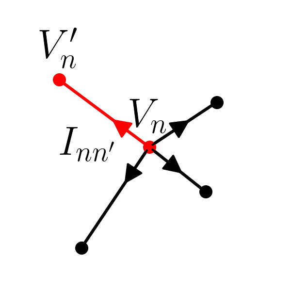
We next demonstrate that a transmission line network is equivalent to a tight-binding system when each section has the same transit time, . To show this, let us add to the notation a little so that is the voltage at the junction (site), and is the current flowing out of that junction to connected site . is the impedance of the section between sites and . Then the transfer matrix gives
| (S6) |
We can use this to find in terms of and , then apply Kirchhoff’s junction rule, , to get
| (S7) |
Here, the sum over includes the sites which are directly connected to . Identifying , this becomes
| (S8) |
This is a generalised eigenvalue problem, but we can turn it into the standard form by defining scaled voltages depending on the impedances of the cables connected to site :
| (S9) |
Then we have the tight binding system
| (S10) |
with
| (S11) |
Note that the ‘energy’, is not the frequency, so zero energy corresponds to finite frequency; indeed the spectrum repeats periodically in frequency.
II S2 Adding Inputs and Outputs
In this section, we show how to add inputs and outputs to the tight binding model derived above. We shall consider an experiment where we connect an input to site , which we model as an ideal voltage source with amplitude in series with an impedance . We measure an output voltage at site , using a detector which is modelled as an ideal voltmeter in parallel with an impedance . The measured output voltage is simply the site voltage .
We start with the detector. From the circuit point of view, this is simply an impedance , which causes an additional current out of the site , with magnitude . The expression from Kirchhoff’s rule for site is then modified to
| (S12) |
since . Now scaling the voltages as in Eq.(S9), the tight binding equation for site becomes
| (S13) |
where ; the finite impedance leads to an on-site imaginary energy for site .
Doing a similar thing for the source, on site , we get a slightly more complicated result. If the source voltage is , and it has an impedance , there is an extra current flowing into site , , determined by
| (S14) |
subtracting this from the Kirchhoff expression gives
| (S15) |
Rearranging, and scaling, we get
| (S16) |
where and . The input adds an on-site imaginary energy and a driving term at site .
We now have a matrix system which takes the form
| (S17) |
where the ‘Hamiltonian’ is the same as in Eq(S10), and is diagonal with the only entries the loss terms and on sites and . The driving term has the single entry on site .
We can diagonalise to find its eigenvalues , and eigenvectors . Then where is the unitary with matrix elements and is a diagonal matrix with . This can be used to invert to get the Green’s function
| (S18) |
so that
| (S19) |
With this, we can relate the output and input voltages for the case where the input and output impedances are infinite, so the loss terms, and are zero:
| (S20) |
However, we really want to find , to deal with the case where there are finite losses. Since has only two non-zero entries, this can be obtained using the Sherman Morrison formula twice. A somewhat involved calculation leads to
| (S21) |
Then
| (S22) |
or, in terms of the unscaled physical quantities,
| (S23) |
For a single port measurement, connecting only to site and measuring to obtain the complex reflectance, we put and get
| (S24) |
However, we can also think of the circuit as simply a potential divider, with the input connected across the input impedance in series with an effective impedance representing the network. In these terms, we get
| (S25) |
so the network impedance is just
| (S26) |
Hence
| (S27) |
which is the unbroadened local density of states on site . In practice, the delta function peaks are broadened by the small resistive losses within the cables.
III S3 Experimental Details
We make our experimental structures using two types of coaxial cable: RG58 and RG62, with impedances of, respectively, 50 and 93. In order to obtain the mapping onto the tight binding Hamiltonian, and thus chiral symmetry, it is essential that the transmission time, , in each section of the cable is the same. For our choice of zero energy at MHz, this corresponds to nominal cable lengths of approximately 41cm and 55cm for the RG58 and RG62 cables, as they have different propagation speeds. However, to obtain the accurate chiral symmetry in our results, it was necessary to consider the contribution of the SMA connectors used to join the cables, which all have impedance. To account for these, the RG58 cables were shortened and the RG62 cables lengthened, such that, in a structure where they alternate, the transmission times in the 50 and 93 sections were the same. However double sections of the same cable type are then the wrong length, and the RG62 doubles contain a pair of 50 connectors in the middle. We avoided this problem by using special double length cables of each type. It is clearly possible also to make triple and greater lengths, but instead we restricted our random sequences to those containing no more than pair repeats.
Radio frequency spectra were obtained using a vector network analyser (NanoVNA V2 Plus4). Our results use two types of measurements. We find the impedance, and thus the local density of states, using a single port measurement of the parameter. The structure impedance is then given by
| (S28) |
where is the output impedance of the VNA. The value of the transmittance, , is obtained directly from a two port measurement between the ends of the cable. The adjustments to the cable lengths to account for the connectors, as described above, moves the effective junctions, and hence the sites in the tight binding model, to the points where the RG62 cables enter there SMA connectors. In the impedance measurements on the terminated chains, we accounted for this by calculating the correction to the impedance due to the transmission through the SMA connector between the physical junction with the VNA and the effective site position. At the opposite end to the measurement, the length of the terminating cable also needed to be modified, so that the final site corresponds to the end of the cable. For an RG62 termination, we simply removed the connector at the end, while in the RG58 case a slightly longer cable accounted for the pair of SMA connectors required to obtain the correct position.
