跳到论文正文
W Papers独立论文阅读器 arXiv:2311.08871 论文正文 计算阅读时间 · 0%
引用这篇论文根据当前论文元数据生成,正式投稿前建议核对。


A short note on super-hedging an arbitrary number of European options with integer-valued strategies

Dorsaf Cherif       Meriam EL MANSOUR       Emmanuel LEPINETTE Faculty of Sciences of Tunis, Tunisia.
Email: dorsaf-cherif@hotmail.fr
Ceremade, UMR CNRS 7534, Paris Dauphine University, PSL National Research, Place du Maréchal De Lattre De Tassigny,
75775 Paris cedex 16, France and
Faculty of Sciences of Tunis, Tunisia.
Email: elmansour@ceremade.dauphine.fr
Ceremade, UMR CNRS 7534, Paris Dauphine University, PSL National Research, Place du Maréchal De Lattre De Tassigny,
75775 Paris cedex 16, France and
Gosaef, Faculty of Sciences of Tunis, Tunisia.
Email: emmanuel.lepinette@ceremade.dauphine.fr

Abstract

The usual theory of asset pricing in finance assumes that the financial strategies, i.e. the quantity of risky assets to invest, are real-valued so that they are not integer-valued in general, see the Black and Scholes model for instance. This is clearly contrary to what it is possible to do in the real world. Surprisingly, it seems that there is no many contributions in that direction in the literature, except for a finite number of states. In this paper, for arbitrary ΩΩ\Omega, we show that, in discrete-time, it is possible to evaluate the minimal super-hedging price when we restrict ourselves to integer-valued strategies. To do so, we only consider terminal claims that are continuous piecewise affine functions of the underlying asset. We formulate a dynamic programming principle that can be directly implemented on an historical data and which also provides the optimal integer-valued strategy. The problem with general payoffs remains open but should be solved with the same approach.

keywords:
Super-hedging prices–European options–Integer-valued strategies–Optimal super-hedging prices–Dynamic programming principle.

MSC: 60-08, 60H30, 90-05, 91-05, 91-10, 91-G15

1 Introduction

The problem of super-hedging a European claim, such as a call option, is very classical in mathematical finance but it has only been solved for real-valued strategies so that the optimal strategy, corresponding to the minimal hedging or super-hedging price, is not integer-valued contrary to what it is allowed to do in the real life. This is why we propose to solve the problem of super-hedging a European claim with integer-valued financial strategies.

Actually, the main contribution in the literature for integer-valued financial strategies is the paper [12] where a finite set of states ΩΩ\Omega is considered. In this setting, the authors adapt the usual theory for the real-valued strategies to the integer-valued ones, i.e. they introduce a no-arbitrage condition which is equivalent to the existence of a risk-neutral probability measure and show that the minimal super-hedging price may be characterized through the martingale measures similarly to the usual case with real-valued strategies. See also [7] where ΩΩ\Omega is finite. The general case with an arbitrary state space ΩΩ\Omega is still an open problem. Also, portfolio optimization problems of Markowitz type are considered in [2], [3], [5].

Let us recall that the usual approach of pricing assumes that the financial market model satisfies a no-arbitrage condition NA, which is equivalent to the existence of a risk-neutral probability measure Q𝑄Q under which the discounted asset prices are martingales, see the Dalang-Morton-Willinger theorem [8]. Under NA, we may show that there exists a minimal super-hedging price P0∗​(ξT)superscriptsubscript𝑃0subscript𝜉𝑇P_{0}^{*}(\xi_{T}) for the European claim ξT≥0subscript𝜉𝑇0\xi_{T}\geq 0 given by

P0∗​(ξT)=supQ∈ℳ​(P)EQ​(ξT),superscriptsubscript𝑃0subscript𝜉𝑇subscriptsupremum𝑄ℳ𝑃subscript𝐸𝑄subscript𝜉𝑇\displaystyle P_{0}^{*}(\xi_{T})=\sup_{Q\in{\cal M}(P)}E_{Q}(\xi_{T}), (1.1)

where ℳ​(P)ℳ𝑃{\cal M}(P) is the set of all risk-neutral probability measures equivalent to the initial probability measure P𝑃P of the model. Here, we suppose that the risk-free interest rate of the model is r=0𝑟0r=0. Recall that the formula above holds in discrete time but also in continuous time with extra-conditions on the model. Indeed, the no-arbitrage condition needs to be strenghtened and it is only equivalent to the existence of Q∼Psimilar-to𝑄𝑃Q\sim P under which discounted asset prices are local martingales, see [9], [10], [11].

In any case, the optimal strategy that achieves the minimal super-hedging price (1.1) is not, in general, integer-valued. The typical example is the continuous-time Black and Scholes model where the so-called delta-hedging strategy for the European call is explicit and lies in the set [0,1]∖{0,1}0101[0,1]\setminus\{0,1\}, see [4].

Clearly, a new approach is necessary to compute the super-hedging prices for only integer-valued financial strategies. We follow the ideas developed in [6] where the problem is initially solved without any no-arbitrage conditions. Then, a no-arbitrage condition AIP naturally appears and means that the infimum price of the zero claim (non negative claims more generally) is not −∞-\infty. This condition is clearly necessary for numerical computations. Actually, it is shown that AIP is equivalent to the property that the infimum super-hedging price of any non negative claim is non negative, as observed in the real markets. In our paper, we do not explicitly suppose such a no-arbitrage condition but the form of the conditional supports of the asset price we assume implies this condition for the model with real-valued strategies.

Our paper is a first attempt to compute super-hedging prices with only integer-valued financial strategies. We restrict ourselves to payoffs which are piecewise affine functions of the underlying asset and we assume specific conditional supports for the asset prices. The problem for general payoff functions remains open but we conjecture that our proposed method can be adapted with more technicalities. Also, problems such as characterizations of the no-arbitrage condition NA with only integer-valued strategies or generalization of our work to arbitrary conditional supports of the asset prices remains open if ΩΩ\Omega is not finite.

Notations If A⊂𝐑𝐴𝐑A\subset{\bf R} is a random subset of 𝐑𝐑{\bf R} and ℱℱ{\cal F} is a σ𝜎\sigma-algebra, we denote by 𝕃0​(A,ℱ)superscript𝕃0𝐴ℱ\mathbb{L}^{0}(A,{\cal F}) the family of all ℱℱ{\cal F}-measurable random variables X𝑋X on the probability space (Ω,ℱ,P)Ωℱ𝑃(\Omega,{\cal F},P) such that X∈A𝑋𝐴X\in A a.s..

2 The super-hedging problem:

We consider n≥1𝑛1n\geq 1 options that we want to super-replicate in discrete time t={0,…​T}.𝑡0…𝑇t=\{0,...T\}. Let (Ω,(ℱt)0≤t≤T)Ωsubscriptsubscriptℱ𝑡0𝑡𝑇(\Omega,(\mathcal{F}_{t})_{0\leq t\leq T}) be a stochastic basis where (ℱt)0≤t≤Tsubscriptsubscriptℱ𝑡0𝑡𝑇(\mathcal{F}_{t})_{0\leq t\leq T} is supposed to be complete. We consider a financial market model composed of two assets. We suppose, without loss of generality, that the risk-free asset is St0=1superscriptsubscript𝑆𝑡01S_{t}^{0}=1 for all t∈{0,…​T},𝑡0…𝑇t\in\{0,...T\}, while the risky asset price is described by a stochastic process S=(St)0≤t≤T.𝑆subscriptsubscript𝑆𝑡0𝑡𝑇S=(S_{t})_{0\leq t\leq T}. Recall that a self-financing portfolio process (Vt)0≤t≤Tsubscriptsubscript𝑉𝑡0𝑡𝑇(V_{t})_{0\leq t\leq T} satisfies by definition:

Δ​Vt=Vt−Vt−1=θt−1​Δ​St,t=1,⋯,T,formulae-sequenceΔsubscript𝑉𝑡subscript𝑉𝑡subscript𝑉𝑡1subscript𝜃𝑡1Δsubscript𝑆𝑡𝑡1⋯𝑇\Delta V_{t}=V_{t}-V_{t-1}=\theta_{t-1}\Delta S_{t},\quad t=1,\cdots,T,

where θt−1subscript𝜃𝑡1\theta_{t-1} is ℱt−1subscriptℱ𝑡1{\cal F}_{t-1}-measurable and represents the number of risky assets of the portfolio.

In this paper, we consider European options whose payoffs are of the form ξT=g​(ST)∈𝕃0​(𝐑,ℱT),subscript𝜉𝑇𝑔subscript𝑆𝑇superscript𝕃0𝐑subscriptℱ𝑇\xi_{T}=g(S_{T})\in\mathbb{L}^{0}({\bf R},\mathcal{F}_{T}), where g𝑔g is a continuous piecewise affine function. The typical example is the European call option, i.e. g​(x)=(x−K)+𝑔𝑥superscript𝑥𝐾g(x)=(x-K)^{+}, K>0𝐾0K>0. Our goal is to compute the set of all super-hedging prices of ξTsubscript𝜉𝑇\xi_{T}, i.e the set of all V0subscript𝑉0V_{0}, initial values of self-financing portfolio processes (Vt)0≤t≤Tsubscriptsubscript𝑉𝑡0𝑡𝑇(V_{t})_{0\leq t\leq T}, such that VT≥ξTsubscript𝑉𝑇subscript𝜉𝑇V_{T}\geq\xi_{T} almost surely. Contrarily to what it is usual to do in the literature, we restrict ourselves to the case of integer-valued strategies, i.e θt∈𝐙subscript𝜃𝑡𝐙\theta_{t}\in{\bf Z} almost surely, for all t∈{0,…​T},𝑡0…𝑇t\in\{0,...T\}, where 𝐙=ℕ∪(−ℕ)𝐙ℕℕ{\bf Z}=\mathbb{N}\cup(-\mathbb{N}) and ℕℕ\mathbb{N} is the set of all non negative integers. In the case of super-hedging an arbitrary number of options n≥1,𝑛1n\geq 1, the problem reads as VT≥n​ξT, a.s.subscript𝑉𝑇𝑛subscript𝜉𝑇 a.s.V_{T}\geq n\xi_{T},\text{~{}a.s.} and it is clearly interesting to analyse the impact of n𝑛n on the strategies and the infimum prices, as linearity is not necessarily preserved with respect to the quantity n𝑛n of claims.

To solve this problem, we follow the approach of [6] and [1] that we adapt to integer-valued strategies. To do so, we first solve backwardly the super-hedging problem between two dates t−1𝑡1t-1 and t,𝑡t, and we show that the procedure may be propagated backwardly as the minimal super-hedging price we obtain at time t−1𝑡1t-1 is still a continuous piecewise affine payoff function of the underlying asset. It is then possible to deduce the minimal super-hedging price at time t=0𝑡0t=0 by induction.

3 The super-hedging problem.

Let t≤T𝑡𝑇t\leq T and gtsubscript𝑔𝑡g_{t} be a continuous piecewise affine function, i.e. there exists a subdivision 0=a0<a1<…<an−1<an=∞0subscript𝑎0subscript𝑎1…subscript𝑎𝑛1subscript𝑎𝑛0=a_{0}<a_{1}<...<a_{n-1}<a_{n}=\infty of [0,∞]0[0,\infty] such that gtsubscript𝑔𝑡g_{t} is an affine function on the interval [ai,ai+1),∀i∈{0,…,n−1}.subscript𝑎𝑖subscript𝑎𝑖1for-all𝑖0…𝑛1[a_{i},a_{i+1}),\forall i\in\{0,...,n-1\}. As the asset prices are non negative, we suppose without loss of generality that a0=0.subscript𝑎00a_{0}=0. We first solve the one step problem: find Vt−1subscript𝑉𝑡1V_{t-1} and the strategy θt−1∈𝕃0​(𝐑,ℱt−1)subscript𝜃𝑡1superscript𝕃0𝐑subscriptℱ𝑡1\theta_{t-1}\in\mathbb{L}^{0}({\bf R},{\cal F}_{t-1}) such that:

Vt−1+θt−1​Δ​St≥gt​(St),a.s..formulae-sequencesubscript𝑉𝑡1subscript𝜃𝑡1Δsubscript𝑆𝑡subscript𝑔𝑡subscript𝑆𝑡asV_{t-1}+\theta_{t-1}\Delta S_{t}\geq g_{t}(S_{t}),\,{\rm a.s..}

This is equivalent to:

Vt−1subscript𝑉𝑡1\displaystyle V_{t-1} ≥\displaystyle\geq gt​(St)−θt−1​Δ​St,subscript𝑔𝑡subscript𝑆𝑡subscript𝜃𝑡1Δsubscript𝑆𝑡\displaystyle g_{t}(S_{t})-\theta_{t-1}\Delta S_{t},
⇔Vt−1⇔absentsubscript𝑉𝑡1\displaystyle\Leftrightarrow V_{t-1} ≥\displaystyle\geq gt​(St)−θt−1​St+θt−1​St−1,subscript𝑔𝑡subscript𝑆𝑡subscript𝜃𝑡1subscript𝑆𝑡subscript𝜃𝑡1subscript𝑆𝑡1\displaystyle g_{t}(S_{t})-\theta_{t-1}S_{t}+\theta_{t-1}S_{t-1},
⇔Vt−1⇔absentsubscript𝑉𝑡1\displaystyle\Leftrightarrow V_{t-1} ≥\displaystyle\geq ess​supℱt−1⁡(gt​(St)−θt−1​St)+θt−1​St−1.subscriptesssupsubscriptℱ𝑡1subscript𝑔𝑡subscript𝑆𝑡subscript𝜃𝑡1subscript𝑆𝑡subscript𝜃𝑡1subscript𝑆𝑡1\displaystyle\operatorname{ess\;sup}_{\mathcal{F}_{t-1}}(g_{t}(S_{t})-\theta_{t-1}S_{t})+\theta_{t-1}S_{t-1}.

Recall that the condition essentiel supremum ess​supℱt−1⁡(Γ)subscriptesssupsubscriptℱ𝑡1Γ\operatorname{ess\;sup}_{\mathcal{F}_{t-1}}(\Gamma), for a familly of random variables ΓΓ\Gamma, is the smallest random variable that dominates a.s. any γ∈Γ𝛾Γ\gamma\in\Gamma, see the definition in [6]. Equivalently, we may show that:

Vt−1≥Vt−1​(θt−1):=supx∈suppℱt−1⁡(St)​(gt​(x)−θt−1​x)+θt−1​St−1,subscript𝑉𝑡1subscript𝑉𝑡1subscript𝜃𝑡1assign𝑥subscriptsuppsubscriptℱ𝑡1subscript𝑆𝑡supremumsubscript𝑔𝑡𝑥subscript𝜃𝑡1𝑥subscript𝜃𝑡1subscript𝑆𝑡1V_{t-1}\geq V_{t-1}(\theta_{t-1}):=\underset{x\in\operatorname{supp}_{\mathcal{F}_{t-1}}(S_{t})}{\sup}(g_{t}(x)-\theta_{t-1}x)+\theta_{t-1}S_{t-1}, (3.2)

where suppℱt−1⁡(St)subscriptsuppsubscriptℱ𝑡1subscript𝑆𝑡\operatorname{supp}_{\mathcal{F}_{t-1}}(S_{t}) is the conditional support of Stsubscript𝑆𝑡S_{t} knowing ℱt−1subscriptℱ𝑡1\mathcal{F}_{t-1}, see [6] and [13] for the definition and the proof of the inequality above.

In the following, we suppose that there exist two deterministic numbers kt−1d∈(0,1)superscriptsubscript𝑘𝑡1𝑑01k_{t-1}^{d}\in(0,1) and kt−1u∈(1,∞)superscriptsubscript𝑘𝑡1𝑢1k_{t-1}^{u}\in(1,\infty) such that suppℱt−1⁡(St)=[kt−1d​St−1,kt−1u​St−1].subscriptsuppsubscriptℱ𝑡1subscript𝑆𝑡superscriptsubscript𝑘𝑡1𝑑subscript𝑆𝑡1superscriptsubscript𝑘𝑡1𝑢subscript𝑆𝑡1\operatorname{supp}_{\mathcal{F}_{t-1}}(S_{t})=[k_{t-1}^{d}S_{t-1},k_{t-1}^{u}S_{t-1}]. This model may be seen as a generalization of the Binomial model and the conditions imposed on the coefficients kt−1dsuperscriptsubscript𝑘𝑡1𝑑k_{t-1}^{d} and kt−1usuperscriptsubscript𝑘𝑡1𝑢k_{t-1}^{u} are equivalent to the weak no-arbitrage condition AIP, see [6]. In particular, we have:

Vt−1​(θt−1)=supx∈[kt−1d​St−1,kt−1u​St−1]​(gt​(x)−θt−1​x)+θt−1​St−1∈𝕃0​(𝐑,ℱt−1).subscript𝑉𝑡1subscript𝜃𝑡1𝑥superscriptsubscript𝑘𝑡1𝑑subscript𝑆𝑡1superscriptsubscript𝑘𝑡1𝑢subscript𝑆𝑡1supremumsubscript𝑔𝑡𝑥subscript𝜃𝑡1𝑥subscript𝜃𝑡1subscript𝑆𝑡1superscript𝕃0𝐑subscriptℱ𝑡1V_{t-1}(\theta_{t-1})=\underset{x\in[k_{t-1}^{d}S_{t-1},k_{t-1}^{u}S_{t-1}]}{\sup}(g_{t}(x)-\theta_{t-1}x)+\theta_{t-1}S_{t-1}\in\mathbb{L}^{0}({\bf R},{\cal F}_{t-1}).

We define Vt−1∗superscriptsubscript𝑉𝑡1V_{t-1}^{*} as the infimum of all super-hedging prices at time t−1𝑡1t-1 over all integer-valued strategies in 𝐙𝐙{\bf Z}, i.e.

Vt−1∗:=ess​infθt−1∈𝕃0​(𝐙,ℱt−1)​Vt−1​(θt−1).assignsuperscriptsubscript𝑉𝑡1subscript𝜃𝑡1superscript𝕃0𝐙subscriptℱ𝑡1essinfsubscript𝑉𝑡1subscript𝜃𝑡1V_{t-1}^{*}:=\underset{\theta_{t-1}\in\mathbb{L}^{0}({\bf Z},\mathcal{F}_{t-1})}{\operatorname{ess\;inf}}V_{t-1}(\theta_{t-1}).
Lemma 3.1.

We have

Vt−1∗=infθ∈𝐙​Vt−1​(θ).superscriptsubscript𝑉𝑡1𝜃𝐙infimumsubscript𝑉𝑡1𝜃V_{t-1}^{*}=\underset{\theta\in{\bf Z}}{\inf}V_{t-1}(\theta). (3.3)
Proof.

Let us define γ=infθ∈𝐙​Vt−1​(θ)∈L0​(𝐑,ℱt−1)𝛾𝜃𝐙infimumsubscript𝑉𝑡1𝜃superscript𝐿0𝐑subscriptℱ𝑡1\gamma=\underset{\theta\in{\bf Z}}{\inf}V_{t-1}(\theta)\in L^{0}({\bf R},{\cal F}_{t-1}), see [6]. As Vt−1∗≤Vt−1​(θ),superscriptsubscript𝑉𝑡1subscript𝑉𝑡1𝜃V_{t-1}^{*}\leq V_{t-1}(\theta), for all θ∈𝐙𝜃𝐙\theta\in{\bf Z}, we get that Vt−1∗≤infθ∈𝐙​Vt−1​(θ)=γ.superscriptsubscript𝑉𝑡1𝜃𝐙infimumsubscript𝑉𝑡1𝜃𝛾V_{t-1}^{*}\leq\underset{\theta\in{\bf Z}}{\inf}V_{t-1}(\theta)=\gamma. On the other hand, if θt−1∈𝕃0​(𝐙,ℱt−1),subscript𝜃𝑡1superscript𝕃0𝐙subscriptℱ𝑡1\theta_{t-1}\in\mathbb{L}^{0}({\bf Z},\mathcal{F}_{t-1}), then:

θt−1subscript𝜃𝑡1\displaystyle\theta_{t-1} =\displaystyle= ∑θ∈Z​θ​1{θt−1=θ},𝜃𝑍𝜃subscript1subscript𝜃𝑡1𝜃\displaystyle\underset{\theta\in Z}{\sum}\theta 1_{\{\theta_{t-1}=\theta\}},
Vt−1​(θt−1)subscript𝑉𝑡1subscript𝜃𝑡1\displaystyle V_{t-1}(\theta_{t-1}) =\displaystyle= ∑θ∈Z​Vt−1​(θ)​1{θt−1=θ}≥∑θ∈Z​γ​1{θt−1=θ}=γ.𝜃𝑍subscript𝑉𝑡1𝜃subscript1subscript𝜃𝑡1𝜃𝜃𝑍𝛾subscript1subscript𝜃𝑡1𝜃𝛾\displaystyle\underset{\theta\in Z}{\sum}V_{t-1}(\theta)1_{\{\theta_{t-1}=\theta\}}\geq\underset{\theta\in Z}{\sum}\gamma 1_{\{\theta_{t-1}=\theta\}}=\gamma.

We deduce that Vt−1∗≥γsuperscriptsubscript𝑉𝑡1𝛾V_{t-1}^{*}\geq\gamma and the conclusion follows. ∎

In the following, we first solve the super-hedging problem between two dates.

Theorem 3.2 (One step problem).

Let us consider t∈{1,…,T}𝑡1…𝑇t\in\{1,...,T\} and suppose that ξt=gt​(St)subscript𝜉𝑡subscript𝑔𝑡subscript𝑆𝑡\xi_{t}=g_{t}(S_{t}) where gtsubscript𝑔𝑡g_{t} is a continuous piecewise affine function. Moreover, we assume that there exists two deterministic numbers kt−1d∈(0,1)superscriptsubscript𝑘𝑡1𝑑01k_{t-1}^{d}\in(0,1) and kt−1u∈(1,∞)superscriptsubscript𝑘𝑡1𝑢1k_{t-1}^{u}\in(1,\infty) such that

suppℱt−1⁡(St)=[kt−1d​St−1,kt−1u​St−1].subscriptsuppsubscriptℱ𝑡1subscript𝑆𝑡superscriptsubscript𝑘𝑡1𝑑subscript𝑆𝑡1superscriptsubscript𝑘𝑡1𝑢subscript𝑆𝑡1\operatorname{supp}_{\mathcal{F}_{t-1}}(S_{t})=[k_{t-1}^{d}S_{t-1},k_{t-1}^{u}S_{t-1}].

Then, Vt−1∗=gt−1​(St−1)subscriptsuperscript𝑉𝑡1subscript𝑔𝑡1subscript𝑆𝑡1V^{*}_{t-1}=g_{t-1}(S_{t-1}) where gt−1subscript𝑔𝑡1g_{t-1} is a continuous piecewise linear function.

Proof.

By assumption, there exist a subdivision (ai)i=0,⋯,nsubscriptsubscript𝑎𝑖𝑖0⋯𝑛(a_{i})_{i=0,\cdots,n} of [0,∞]0[0,\infty], with a0=0<a1<…<an−1<an=∞subscript𝑎00subscript𝑎1…subscript𝑎𝑛1subscript𝑎𝑛a_{0}=0<a_{1}<...<a_{n-1}<a_{n}=\infty, such that gtsubscript𝑔𝑡g_{t} is an affine function on each interval. Let us define

xi​(St−1)=(kt−1d​St−1∨ai)∧kt−1u​St−1,i=0,⋯,n.formulae-sequencesubscript𝑥𝑖subscript𝑆𝑡1superscriptsubscript𝑘𝑡1𝑑subscript𝑆𝑡1subscript𝑎𝑖superscriptsubscript𝑘𝑡1𝑢subscript𝑆𝑡1𝑖0⋯𝑛x_{i}(S_{t-1})=(k_{t-1}^{d}S_{t-1}\vee a_{i})\wedge k_{t-1}^{u}S_{t-1},\quad i=0,\cdots,n.

It is straightforward that

Vt−1​(θt−1)=supi=0,⋯,n​[gt​(xi​(St−1))−θt−1​xi​(St−1)]+θt−1​St−1.subscript𝑉𝑡1subscript𝜃𝑡1𝑖0⋯𝑛supremumdelimited-[]subscript𝑔𝑡subscript𝑥𝑖subscript𝑆𝑡1subscript𝜃𝑡1subscript𝑥𝑖subscript𝑆𝑡1subscript𝜃𝑡1subscript𝑆𝑡1V_{t-1}(\theta_{t-1})=\underset{i=0,\cdots,n}{\sup}\left[g_{t}(x_{i}(S_{t-1}))-\theta_{t-1}x_{i}(S_{t-1})\right]+\theta_{t-1}S_{t-1}.

Note that x0​(St−1)=kd​St−1subscript𝑥0subscript𝑆𝑡1superscript𝑘𝑑subscript𝑆𝑡1x_{0}(S_{t-1})=k^{d}S_{t-1} and xn​(St−1)=ku​St−1subscript𝑥𝑛subscript𝑆𝑡1superscript𝑘𝑢subscript𝑆𝑡1x_{n}(S_{t-1})=k^{u}S_{t-1} and some terms of the sequence (xi)isubscriptsubscript𝑥𝑖𝑖(x_{i})_{i} may coincide. Let us define the functions

hi​(θt−1,St−1)=gt​(xi​(St−1))+θt−1​(St−1−xi​(St−1)),i=0,⋯,n.formulae-sequencesuperscriptℎ𝑖subscript𝜃𝑡1subscript𝑆𝑡1subscript𝑔𝑡subscript𝑥𝑖subscript𝑆𝑡1subscript𝜃𝑡1subscript𝑆𝑡1subscript𝑥𝑖subscript𝑆𝑡1𝑖0⋯𝑛h^{i}(\theta_{t-1},S_{t-1})=g_{t}(x_{i}(S_{t-1}))+\theta_{t-1}(S_{t-1}-x_{i}(S_{t-1})),\,i=0,\cdots,n.

The slopes of the affine functions θt−1↦hi​(θt−1,St−1)maps-tosubscript𝜃𝑡1superscriptℎ𝑖subscript𝜃𝑡1subscript𝑆𝑡1\theta_{t-1}\mapsto h^{i}(\theta_{t-1},S_{t-1}) are given by the non decreasing sequence (St−1−xi​(St−1))i=n,n−1,⋯,0subscriptsubscript𝑆𝑡1subscript𝑥𝑖subscript𝑆𝑡1𝑖𝑛𝑛1⋯0(S_{t-1}-x_{i}(S_{t-1}))_{i=n,n-1,\cdots,0} such that St−1−xn​(St−1)<0subscript𝑆𝑡1subscript𝑥𝑛subscript𝑆𝑡10S_{t-1}-x_{n}(S_{t-1})<0 and St−1−x0​(St−1)>0.subscript𝑆𝑡1subscript𝑥0subscript𝑆𝑡10S_{t-1}-x_{0}(S_{t-1})>0.

By ordering the indices in the decreasing order, we obtain (n+1)𝑛1(n+1) affine functions θt−1↦hi​(θt−1)maps-tosubscript𝜃𝑡1superscriptℎ𝑖subscript𝜃𝑡1\theta_{t-1}\mapsto h^{i}(\theta_{t-1}) for i∈{n,n−1,…,1,0}𝑖𝑛𝑛1…10i\in\{n,n-1,...,1,0\} with increasing slopes (St−1−xi)i∈{n,n−1,…,1,0},subscriptsubscript𝑆𝑡1subscript𝑥𝑖𝑖𝑛𝑛1…10(S_{t-1}-x_{i})_{i\in\{n,n-1,...,1,0\}}, such that: St−1−xn<0subscript𝑆𝑡1subscript𝑥𝑛0S_{t-1}-x_{n}<0 and St−1−x0>0.subscript𝑆𝑡1subscript𝑥00S_{t-1}-x_{0}>0. Therefore, the mapping Vt−1:θt−1↦supi=n,…,0​hi​(θt−1,St−1):subscript𝑉𝑡1maps-tosubscript𝜃𝑡1𝑖𝑛…0supremumsuperscriptℎ𝑖subscript𝜃𝑡1subscript𝑆𝑡1V_{t-1}:\theta_{t-1}\mapsto\underset{i=n,...,0}{\sup}h^{i}(\theta_{t-1},S_{t-1}) is a piecewise affine function, i.e. there exists a subdivision:

−∞=α0<α1​(St−1)≤…≤αm−1​(St−1)<αm=∞subscript𝛼0subscript𝛼1subscript𝑆𝑡1…subscript𝛼𝑚1subscript𝑆𝑡1subscript𝛼𝑚-\infty=\alpha_{0}<\alpha_{1}(S_{t-1})\leq...\leq\alpha_{m-1}(S_{t-1})<\alpha_{m}=\infty

such that Vt−1subscript𝑉𝑡1V_{t-1} is an affine function of θt−1subscript𝜃𝑡1\theta_{t-1} on each interval [αi​(St−1),αi+1​(St−1)]subscript𝛼𝑖subscript𝑆𝑡1subscript𝛼𝑖1subscript𝑆𝑡1[\alpha_{i}(S_{t-1}),\alpha_{i+1}(S_{t-1})], i=0,⋯,m−1𝑖0⋯𝑚1i=0,\cdots,m-1. Note that the function Vt−1subscript𝑉𝑡1V_{t-1} is convex in θt−1subscript𝜃𝑡1\theta_{t-1} and the elements of the partition define the intersection points between two distinct and successive graphs of the affine functions hi+1​(θt−1),hi​(θt−1)superscriptℎ𝑖1subscript𝜃𝑡1superscriptℎ𝑖subscript𝜃𝑡1h^{i+1}(\theta_{t-1}),h^{i}(\theta_{t-1}). So, there exists θt−1∗∈[α1​(St−1)−1,…,αm−1​(St−1)+1]∩𝐙superscriptsubscript𝜃𝑡1subscript𝛼1subscript𝑆𝑡11…subscript𝛼𝑚1subscript𝑆𝑡11𝐙\theta_{t-1}^{*}\in[\alpha_{1}(S_{t-1})-1,...,\alpha_{m-1}(S_{t-1})+1]\cap{\bf Z} such that:

infθt−1∈𝐙​Vt−1​(θt−1)=Vt−1​(θt−1∗).subscript𝜃𝑡1𝐙infimumsubscript𝑉𝑡1subscript𝜃𝑡1subscript𝑉𝑡1superscriptsubscript𝜃𝑡1\underset{\theta_{t-1}\in{\bf Z}}{\inf}V_{t-1}(\theta_{t-1})=V_{t-1}(\theta_{t-1}^{*}).

It remains to evaluate α1​(St−1)subscript𝛼1subscript𝑆𝑡1\alpha_{1}(S_{t-1}) and αm−1​(St−1)subscript𝛼𝑚1subscript𝑆𝑡1\alpha_{m-1}(S_{t-1}). To do so, let us solve the equations hi​(α)=hj​(α)superscriptℎ𝑖𝛼superscriptℎ𝑗𝛼h^{i}(\alpha)=h^{j}(\alpha), i,j=0,…,mformulae-sequence𝑖𝑗0…𝑚i,j=0,...,m and xi≠xjsubscript𝑥𝑖subscript𝑥𝑗x_{i}\neq x_{j}. Since we suppose that xi−xj≠0,subscript𝑥𝑖subscript𝑥𝑗0x_{i}-x_{j}\neq 0, we get that

α=gt​(xi)−gt​(xj)xi−xj.𝛼subscript𝑔𝑡subscript𝑥𝑖subscript𝑔𝑡subscript𝑥𝑗subscript𝑥𝑖subscript𝑥𝑗\alpha=\frac{g_{t}(x_{i})-g_{t}(x_{j})}{x_{i}-x_{j}}.

We deduce that |α|≤Lt𝛼subscript𝐿𝑡|\alpha|\leq L_{t} where Lt>0subscript𝐿𝑡0L_{t}>0 is a Lipschitz constant of the piecewise affine function gtsubscript𝑔𝑡g_{t}. We deduce that θt−1∗∈[−Lt−1,Lt+1]∩𝐙superscriptsubscript𝜃𝑡1subscript𝐿𝑡1subscript𝐿𝑡1𝐙\theta_{t-1}^{*}\in[-L_{t}-1,L_{t}+1]\cap{\bf Z} and

gt−1​(St−1)=Vt−1​(θt−1∗​(St−1))=minθt−1∈[−Lt−1,Lt+1]∩𝐙​supi=0,⋯,n​hi​(θt−1,St−1).subscript𝑔𝑡1subscript𝑆𝑡1subscript𝑉𝑡1superscriptsubscript𝜃𝑡1subscript𝑆𝑡1subscript𝜃𝑡1subscript𝐿𝑡1subscript𝐿𝑡1𝐙𝑖0⋯𝑛supremumsuperscriptℎ𝑖subscript𝜃𝑡1subscript𝑆𝑡1g_{t-1}(S_{t-1})=V_{t-1}(\theta_{t-1}^{*}(S_{t-1}))=\underset{\theta_{t-1}\in[-L_{t}-1,L_{t}+1]\cap{\bf Z}}{\min}~{}\underset{i=0,\cdots,n}{\sup}h^{i}(\theta_{t-1},S_{t-1}).

We conclude that gt−1subscript𝑔𝑡1g_{t-1} is a continuous piecewise affine function as a minimum of a finite number of continuous piecewise affine functions. ∎

Corollary 3.3.

(The multi-period super-hedging problem) Suppose that, at time T>0𝑇0T>0, the payoff is ξT=gT​(ST)subscript𝜉𝑇subscript𝑔𝑇subscript𝑆𝑇\xi_{T}=g_{T}(S_{T}) where gTsubscript𝑔𝑇g_{T} is a continuous piecewise affine function. Moreover, we assume that there exists deterministic numbers kt−1d∈(0,1)superscriptsubscript𝑘𝑡1𝑑01k_{t-1}^{d}\in(0,1) and kt−1u∈(1,∞)superscriptsubscript𝑘𝑡1𝑢1k_{t-1}^{u}\in(1,\infty) for each t=1,⋯,T𝑡1⋯𝑇t=1,\cdots,T such that we have suppℱt−1⁡(St)=[kt−1d​St−1,kt−1u​St−1].subscriptsuppsubscriptℱ𝑡1subscript𝑆𝑡superscriptsubscript𝑘𝑡1𝑑subscript𝑆𝑡1superscriptsubscript𝑘𝑡1𝑢subscript𝑆𝑡1\operatorname{supp}_{\mathcal{F}_{t-1}}(S_{t})=[k_{t-1}^{d}S_{t-1},k_{t-1}^{u}S_{t-1}]. Then, there exists a minimal super-hedging portfolio process (Vt∗)t=0,⋯,Tsubscriptsubscriptsuperscript𝑉𝑡𝑡0⋯𝑇(V^{*}_{t})_{t=0,\cdots,T} such that VT∗≥ξTsuperscriptsubscript𝑉𝑇subscript𝜉𝑇V_{T}^{*}\geq\xi_{T}. We have Vt∗=g​(t,St)subscriptsuperscript𝑉𝑡𝑔𝑡subscript𝑆𝑡V^{*}_{t}=g(t,S_{t}) where g​(t,⋅)𝑔𝑡⋅g(t,\cdot) is a continuous piecewise affine function given by

g​(t,s)𝑔𝑡𝑠\displaystyle g(t,s) =\displaystyle= minθ∈[−Lt+1−1,Lt+1+1]∩𝐙​supi=0,⋯,n(t+1)​(g​(t+1,xi(t+1)​(s))+θ​(s−xi(t+1)​(s))),𝜃subscript𝐿𝑡11subscript𝐿𝑡11𝐙𝑖0⋯superscript𝑛𝑡1supremum𝑔𝑡1superscriptsubscript𝑥𝑖𝑡1𝑠𝜃𝑠superscriptsubscript𝑥𝑖𝑡1𝑠\displaystyle\underset{\theta\in[-L_{t+1}-1,L_{t+1}+1]\cap{\bf Z}}{\min}~{}\underset{i=0,\cdots,n^{(t+1)}}{\sup}\left(g(t+1,x_{i}^{(t+1)}(s))+\theta(s-x_{i}^{(t+1)}(s))\right),
xi(t+1)​(s)superscriptsubscript𝑥𝑖𝑡1𝑠\displaystyle x_{i}^{(t+1)}(s) =\displaystyle= (ktd​s∨ai(t+1))∧ktu​s,i=0,⋯,n(t+1),formulae-sequencesuperscriptsubscript𝑘𝑡𝑑𝑠superscriptsubscript𝑎𝑖𝑡1superscriptsubscript𝑘𝑡𝑢𝑠𝑖0⋯superscript𝑛𝑡1\displaystyle(k_{t}^{d}s\vee a_{i}^{(t+1)})\wedge k_{t}^{u}s,\quad i=0,\cdots,n^{(t+1)},

where Lt+1subscript𝐿𝑡1L_{t+1} is any Lipschitz constant of the function g​(t+1,⋅)𝑔𝑡1⋅g(t+1,\cdot) and (ai(t+1))i=0,⋯,n(t+1)subscriptsuperscriptsubscript𝑎𝑖𝑡1𝑖0⋯superscript𝑛𝑡1(a_{i}^{(t+1)})_{i=0,\cdots,n^{(t+1)}} is any partition such that a0(t+1)=0<a1(t+1)<…<an(t+1)−1(t+1)<an(t+1)(t+1)=∞superscriptsubscript𝑎0𝑡10superscriptsubscript𝑎1𝑡1…superscriptsubscript𝑎superscript𝑛𝑡11𝑡1superscriptsubscript𝑎superscript𝑛𝑡1𝑡1a_{0}^{(t+1)}=0<a_{1}^{(t+1)}<...<a_{n^{(t+1)}-1}^{(t+1)}<a_{n^{(t+1)}}^{(t+1)}=\infty and g​(t+1,⋅)𝑔𝑡1⋅g(t+1,\cdot) is an affine function on [ai(t+1),ai+1(t+1)]superscriptsubscript𝑎𝑖𝑡1superscriptsubscript𝑎𝑖1𝑡1[a_{i}^{(t+1)},a_{i+1}^{(t+1)}], i≤n(t+1)−1𝑖superscript𝑛𝑡11i\leq n^{(t+1)}-1. The associated super-hedging strategy θ∗superscript𝜃\theta^{*} is given by the argmin of the minimisation problem defining g​(t,⋅)𝑔𝑡⋅g(t,\cdot) in the expression above.

The result above provides a recipe to compute backwardly the minimal super-hedging price at any time, which is the main goal of our paper.

Theorem 3.4.

Let g​(t,x,n)𝑔𝑡𝑥𝑛g(t,x,n) be the price function as given in Corollary 3.3 at time t𝑡t for n≥1𝑛1n\geq 1 units of claims gT​(ST)subscript𝑔𝑇subscript𝑆𝑇g_{T}(S_{T}), i.e. the payoff is ξT=n​gT​(ST)subscript𝜉𝑇𝑛subscript𝑔𝑇subscript𝑆𝑇\xi_{T}=ng_{T}(S_{T}), where gTsubscript𝑔𝑇g_{T} satisfies the conditions of Corollary 3.3. Let g^​(t,x)^𝑔𝑡𝑥\hat{g}(t,x) be the price function for one unit of the claim gT​(ST)subscript𝑔𝑇subscript𝑆𝑇g_{T}(S_{T}) in the model where real-valued strategies are allowed, see [6]. Suppose that the price process S𝑆S satisfies the conditions of Corollary 3.3. Then, g​(t,x,n)n𝑔𝑡𝑥𝑛𝑛\frac{g(t,x,n)}{n} converges to g^​(t,x)^𝑔𝑡𝑥\hat{g}(t,x) as n→∞→𝑛n\to\infty.

Proof.

Note that there exists a constant M>0𝑀0M>0 such that 0≤St≤M0subscript𝑆𝑡𝑀0\leq S_{t}\leq M a.s. for all t=0,⋯,T𝑡0⋯𝑇t=0,\cdots,T. By definition, there exists an integer-valued strategy (θtn)t=0,⋯,T−1subscriptsubscriptsuperscript𝜃𝑛𝑡𝑡0⋯𝑇1(\theta^{n}_{t})_{t=0,\cdots,T-1} such that g​(t,x,n)+∑t=1Tθt−1n​Δ​St≥n​gT​(ST)𝑔𝑡𝑥𝑛superscriptsubscript𝑡1𝑇subscriptsuperscript𝜃𝑛𝑡1Δsubscript𝑆𝑡𝑛subscript𝑔𝑇subscript𝑆𝑇g(t,x,n)+\sum_{t=1}^{T}\theta^{n}_{t-1}\Delta S_{t}\geq ng_{T}(S_{T}). By definition of the smallest price for n𝑛n units of claims with real-valued strategies, we have g^​(t,x,n)=n​g^​(t,x)^𝑔𝑡𝑥𝑛𝑛^𝑔𝑡𝑥\hat{g}(t,x,n)=n\hat{g}(t,x) where g^​(t,x)=g^​(t,x,1)^𝑔𝑡𝑥^𝑔𝑡𝑥1\hat{g}(t,x)=\hat{g}(t,x,1) by linearity of the model [6]. As it is the smallest price, we deduce that n​g^​(t,x)≤g​(t,x,n)𝑛^𝑔𝑡𝑥𝑔𝑡𝑥𝑛n\hat{g}(t,x)\leq g(t,x,n), i.e. g^​(t,x)≤g​(t,x,n)n^𝑔𝑡𝑥𝑔𝑡𝑥𝑛𝑛\hat{g}(t,x)\leq\frac{g(t,x,n)}{n}. On the other hand, still by definition, there exists a real-valued strategy (θtr)t=0,⋯,T−1subscriptsubscriptsuperscript𝜃𝑟𝑡𝑡0⋯𝑇1(\theta^{r}_{t})_{t=0,\cdots,T-1} such that n​g^​(t,x)+∑t=1Tθt−1r​Δ​St≥n​gT​(ST)𝑛^𝑔𝑡𝑥superscriptsubscript𝑡1𝑇subscriptsuperscript𝜃𝑟𝑡1Δsubscript𝑆𝑡𝑛subscript𝑔𝑇subscript𝑆𝑇n\hat{g}(t,x)+\sum_{t=1}^{T}\theta^{r}_{t-1}\Delta S_{t}\geq ng_{T}(S_{T}). We decompose each θt−1r=θ¯t−1r+dt−1subscriptsuperscript𝜃𝑟𝑡1subscriptsuperscript¯𝜃𝑟𝑡1subscript𝑑𝑡1\theta^{r}_{t-1}=\bar{\theta}^{r}_{t-1}+d_{t-1} into θ¯t−1rsubscriptsuperscript¯𝜃𝑟𝑡1\bar{\theta}^{r}_{t-1} the integer part of θt−1rsubscriptsuperscript𝜃𝑟𝑡1\theta^{r}_{t-1} and dt−1=θt−1r−θ¯t−1rsubscript𝑑𝑡1subscriptsuperscript𝜃𝑟𝑡1subscriptsuperscript¯𝜃𝑟𝑡1d_{t-1}=\theta^{r}_{t-1}-\bar{\theta}^{r}_{t-1} the residual term. We observe that |∑t=1Tdt−1​Δ​St|≤2​T​Msuperscriptsubscript𝑡1𝑇subscript𝑑𝑡1Δsubscript𝑆𝑡2𝑇𝑀\left|\sum_{t=1}^{T}d_{t-1}\Delta S_{t}\right|\leq 2TM. We deduce that 2​T​M+n​g^​(t,x)+∑t=1Tθ¯t−1r​Δ​St≥n​gT​(ST)2𝑇𝑀𝑛^𝑔𝑡𝑥superscriptsubscript𝑡1𝑇subscriptsuperscript¯𝜃𝑟𝑡1Δsubscript𝑆𝑡𝑛subscript𝑔𝑇subscript𝑆𝑇2TM+n\hat{g}(t,x)+\sum_{t=1}^{T}\bar{\theta}^{r}_{t-1}\Delta S_{t}\geq ng_{T}(S_{T}) and we deduce by definition that g​(t,x,n)≤2​T​M+n​g^​(t,x)𝑔𝑡𝑥𝑛2𝑇𝑀𝑛^𝑔𝑡𝑥g(t,x,n)\leq 2TM+n\hat{g}(t,x). We finally get the inequality g^​(t,x)≤g​(t,x,n)n≤2​T​Mn+g^​(t,x)^𝑔𝑡𝑥𝑔𝑡𝑥𝑛𝑛2𝑇𝑀𝑛^𝑔𝑡𝑥\hat{g}(t,x)\leq\frac{g(t,x,n)}{n}\leq\frac{2TM}{n}+\hat{g}(t,x). The conclusion follows.

∎

The theorem above is interesting for practitioners. It implies that, if n𝑛n is large enough and if the practitioners only trade integer-valued strategies, then the price of n𝑛n claims gT​(ST)subscript𝑔𝑇subscript𝑆𝑇g_{T}(S_{T}) is approximately n​g^​(t,x)𝑛^𝑔𝑡𝑥n\hat{g}(t,x). This is important for numerical reasons as the computation of g​(t,x,n)𝑔𝑡𝑥𝑛g(t,x,n) is rather time-consuming contrarily to the computation of g^​(t,x)^𝑔𝑡𝑥\hat{g}(t,x), see [6].

3.1 Example in the one step problem: the case of the Call option

At time t=T𝑡𝑇t=T, suppose that the payoff is ξTn=n​g​(ST)superscriptsubscript𝜉𝑇𝑛𝑛𝑔subscript𝑆𝑇\xi_{T}^{n}=ng(S_{T}) where n≥1𝑛1n\geq 1 and g​(x)=(x−K)+𝑔𝑥superscript𝑥𝐾g(x)=(x-K)^{+}, K=500𝐾500K=500. We suppose that suppℱT−1⁡(ST)=[kd​ST−1,ku​ST−1]subscriptsuppsubscriptℱ𝑇1subscript𝑆𝑇superscript𝑘𝑑subscript𝑆𝑇1superscript𝑘𝑢subscript𝑆𝑇1\operatorname{supp}_{\mathcal{F}_{T-1}}(S_{T})=[k^{d}S_{T-1},k^{u}S_{T-1}] for some constants kd,kusuperscript𝑘𝑑superscript𝑘𝑢k^{d},k^{u} such that 0<kd<1<ku0superscript𝑘𝑑1superscript𝑘𝑢0<k^{d}<1<k^{u}. Precisely, we suppose that kd=0.9superscript𝑘𝑑0.9k^{d}=0.9 and ku=1.2superscript𝑘𝑢1.2k^{u}=1.2. Observe that the super-hedging problem VT−1+θT−1​Δ​ST≥n​g​(ST)subscript𝑉𝑇1subscript𝜃𝑇1Δsubscript𝑆𝑇𝑛𝑔subscript𝑆𝑇V_{T-1}+\theta_{T-1}\Delta S_{T}\geq ng(S_{T}) is equivalent to

VT−1≥VT−1​(θT−1)=maxk∈{kd,ku}⁡[n​g​(k​ST−1)−θT−1​k​ST−1]+θT−1​ST−1.subscript𝑉𝑇1subscript𝑉𝑇1subscript𝜃𝑇1subscript𝑘superscript𝑘𝑑superscript𝑘𝑢𝑛𝑔𝑘subscript𝑆𝑇1subscript𝜃𝑇1𝑘subscript𝑆𝑇1subscript𝜃𝑇1subscript𝑆𝑇1\displaystyle V_{T-1}\geq V_{T-1}(\theta_{T-1})=\max_{k\in\{k^{d},k^{u}\}}[ng(kS_{T-1})-\theta_{T-1}kS_{T-1}]+\theta_{T-1}S_{T-1}.

In the following we give the explicit expression of VT−1​(θT−1)=VT−1n​(θT−1)subscript𝑉𝑇1subscript𝜃𝑇1superscriptsubscript𝑉𝑇1𝑛subscript𝜃𝑇1V_{T-1}(\theta_{T-1})=V_{T-1}^{n}(\theta_{T-1}).


If ku≤K/ST−1superscript𝑘𝑢𝐾subscript𝑆𝑇1k^{u}\leq K/S_{T-1}, i.e. ST−1≤K/kusubscript𝑆𝑇1𝐾superscript𝑘𝑢S_{T-1}\leq K/k^{u}, then

VT−1​(θT−1)={θT−1​ST−1​(1−ku)if​θT−1≤0,θT−1​ST−1​(1−kd)if​θT−1≥0.subscript𝑉𝑇1subscript𝜃𝑇1casessubscript𝜃𝑇1subscript𝑆𝑇11superscript𝑘𝑢ifsubscript𝜃𝑇10subscript𝜃𝑇1subscript𝑆𝑇11superscript𝑘𝑑ifsubscript𝜃𝑇10V_{T-1}(\theta_{T-1})=\begin{cases}\theta_{T-1}S_{T-1}(1-k^{u})&\text{if}~{}~{}\theta_{T-1}\leq 0,\\ \theta_{T-1}S_{T-1}(1-k^{d})&\text{if}~{}~{}\theta_{T-1}\geq 0.\end{cases}

Therefore, θT−1∗,n​(ST−1)=0superscriptsubscript𝜃𝑇1𝑛subscript𝑆𝑇10\theta_{T-1}^{*,n}(S_{T-1})=0, and VT−1∗,n​(ST−1)=VT−1​(θT−1∗,n)=0superscriptsubscript𝑉𝑇1𝑛subscript𝑆𝑇1subscript𝑉𝑇1superscriptsubscript𝜃𝑇1𝑛0V_{T-1}^{*,n}(S_{T-1})=V_{T-1}(\theta_{T-1}^{*,n})=0.


If kd≥K/ST−1superscript𝑘𝑑𝐾subscript𝑆𝑇1k^{d}\geq K/S_{T-1}, i.e. ST−1≥K/kdsubscript𝑆𝑇1𝐾superscript𝑘𝑑S_{T-1}\geq K/k^{d},

VT−1​(θT−1)={θT−1​ST−1​(1−ku)+n​ku​ST−1−n​Kif​θT−1≤n,θT−1​ST−1​(1−kd)+n​kd​ST−1−n​Kif​θT−1≥n.subscript𝑉𝑇1subscript𝜃𝑇1casessubscript𝜃𝑇1subscript𝑆𝑇11superscript𝑘𝑢𝑛superscript𝑘𝑢subscript𝑆𝑇1𝑛𝐾ifsubscript𝜃𝑇1𝑛subscript𝜃𝑇1subscript𝑆𝑇11superscript𝑘𝑑𝑛superscript𝑘𝑑subscript𝑆𝑇1𝑛𝐾ifsubscript𝜃𝑇1𝑛V_{T-1}(\theta_{T-1})=\begin{cases}\theta_{T-1}S_{T-1}(1-k^{u})+nk^{u}S_{T-1}-nK&\text{if}~{}~{}\theta_{T-1}\leq n,\\ \theta_{T-1}S_{T-1}(1-k^{d})+nk^{d}S_{T-1}-nK&\text{if}~{}~{}\theta_{T-1}\geq n.\end{cases}

We conclude that θT−1∗,n​(ST−1)=nsuperscriptsubscript𝜃𝑇1𝑛subscript𝑆𝑇1𝑛\theta_{T-1}^{*,n}(S_{T-1})=n, and VT−1∗,n​(ST−1)=n​(ST−1−K)superscriptsubscript𝑉𝑇1𝑛subscript𝑆𝑇1𝑛subscript𝑆𝑇1𝐾V_{T-1}^{*,n}(S_{T-1})=n(S_{T-1}-K).


If kd≤K/ST−1≤kusuperscript𝑘𝑑𝐾subscript𝑆𝑇1superscript𝑘𝑢k^{d}\leq K/S_{T-1}\leq k^{u}, i.e. ST−1∈[K/ku,K/kd]subscript𝑆𝑇1𝐾superscript𝑘𝑢𝐾superscript𝑘𝑑S_{T-1}\in[K/k^{u},K/k^{d}],

VT−1​(θT−1)={θT−1​ST−1​(1−ku)+n​ku​ST−1−n​Kif​θT−1≤n​ku​ST−1−n​KST−1​(ku−kd),θT−1​ST−1​(1−kd)if​θT−1≥n​ku​ST−1−n​KST−1​(ku−kd).subscript𝑉𝑇1subscript𝜃𝑇1casessubscript𝜃𝑇1subscript𝑆𝑇11superscript𝑘𝑢𝑛superscript𝑘𝑢subscript𝑆𝑇1𝑛𝐾ifsubscript𝜃𝑇1𝑛superscript𝑘𝑢subscript𝑆𝑇1𝑛𝐾subscript𝑆𝑇1superscript𝑘𝑢superscript𝑘𝑑subscript𝜃𝑇1subscript𝑆𝑇11superscript𝑘𝑑ifsubscript𝜃𝑇1𝑛superscript𝑘𝑢subscript𝑆𝑇1𝑛𝐾subscript𝑆𝑇1superscript𝑘𝑢superscript𝑘𝑑V_{T-1}(\theta_{T-1})=\begin{cases}\theta_{T-1}S_{T-1}(1-k^{u})+nk^{u}S_{T-1}-nK&\text{if}~{}~{}\theta_{T-1}\leq\frac{nk^{u}S_{T-1}-nK}{S_{T-1}(k^{u}-k^{d})},\\ \theta_{T-1}S_{T-1}(1-k^{d})&\text{if}~{}~{}\theta_{T-1}\geq\frac{nk^{u}S_{T-1}-nK}{S_{T-1}(k^{u}-k^{d})}.\end{cases}

Let us define

αT−1n​(ST−1)superscriptsubscript𝛼𝑇1𝑛subscript𝑆𝑇1\displaystyle\alpha_{T-1}^{n}(S_{T-1}) :=assign\displaystyle:= n​ku​ST−1−n​KST−1​(ku−kd),𝑛superscript𝑘𝑢subscript𝑆𝑇1𝑛𝐾subscript𝑆𝑇1superscript𝑘𝑢superscript𝑘𝑑\displaystyle\frac{nk^{u}S_{T-1}-nK}{S_{T-1}(k^{u}-k^{d})},
fn​(x,ST−1)superscript𝑓𝑛𝑥subscript𝑆𝑇1\displaystyle f^{n}(x,S_{T-1}) :=assign\displaystyle:= x​ST−1​(1−kd)​1{x≥αT−1​(ST−1)}𝑥subscript𝑆𝑇11superscript𝑘𝑑subscript1𝑥subscript𝛼𝑇1subscript𝑆𝑇1\displaystyle xS_{T-1}(1-k^{d})1_{\{x\geq\alpha_{T-1}(S_{T-1})\}}
+(x​ST−1​(1−ku)+n​ku​ST−1−n​K)​1{x<αT−1​(ST−1)}.𝑥subscript𝑆𝑇11superscript𝑘𝑢𝑛superscript𝑘𝑢subscript𝑆𝑇1𝑛𝐾subscript1𝑥subscript𝛼𝑇1subscript𝑆𝑇1\displaystyle+(xS_{T-1}(1-k^{u})+nk^{u}S_{T-1}-nK)1_{\{x<\alpha_{T-1}(S_{T-1})\}}.

We denote by ⌊αT−1n​(ST−1)⌋superscriptsubscript𝛼𝑇1𝑛subscript𝑆𝑇1\lfloor\alpha_{T-1}^{n}(S_{T-1})\rfloor the lower integer part of αT−1nsuperscriptsubscript𝛼𝑇1𝑛\alpha_{T-1}^{n}. Then,

θT−1∗,n​(ST−1)={⌊αT−1n​(ST−1)⌋if​fn​(⌊αT−1​(ST−1)⌋)≤fn​(⌊αT−1​(ST−1)⌋+1),⌊αT−1n​(ST−1)⌋+1otherwise.superscriptsubscript𝜃𝑇1𝑛subscript𝑆𝑇1casessuperscriptsubscript𝛼𝑇1𝑛subscript𝑆𝑇1ifsuperscript𝑓𝑛subscript𝛼𝑇1subscript𝑆𝑇1superscript𝑓𝑛subscript𝛼𝑇1subscript𝑆𝑇11superscriptsubscript𝛼𝑇1𝑛subscript𝑆𝑇11otherwise.\theta_{T-1}^{*,n}(S_{T-1})=\begin{cases}\lfloor\alpha_{T-1}^{n}(S_{T-1})\rfloor&\text{if}~{}~{}f^{n}(\lfloor\alpha_{T-1}(S_{T-1})\rfloor)\leq f^{n}(\lfloor\alpha_{T-1}(S_{T-1})\rfloor+1),\\ \lfloor\alpha_{T-1}^{n}(S_{T-1})\rfloor+1&\text{otherwise.}\end{cases}

So, we have:

VT−1∗,n​(ST−1)superscriptsubscript𝑉𝑇1𝑛subscript𝑆𝑇1\displaystyle V_{T-1}^{*,n}(S_{T-1}) =\displaystyle= (⌊αT−1n​(ST−1)⌋​ST−1​(1−ku)+n​ku​ST−1−n​K)​1GT−1n​(ST−1)superscriptsubscript𝛼𝑇1𝑛subscript𝑆𝑇1subscript𝑆𝑇11superscript𝑘𝑢𝑛superscript𝑘𝑢subscript𝑆𝑇1𝑛𝐾subscript1superscriptsubscript𝐺𝑇1𝑛subscript𝑆𝑇1\displaystyle(\lfloor\alpha_{T-1}^{n}(S_{T-1})\rfloor S_{T-1}(1-k^{u})+nk^{u}S_{T-1}-nK)1_{G_{T-1}^{n}}(S_{T-1})
+(⌊αT−1n⌋+1)​ST−1​(1−kd)​1(GT−1n)c​(ST−1),superscriptsubscript𝛼𝑇1𝑛1subscript𝑆𝑇11superscript𝑘𝑑subscript1superscriptsuperscriptsubscript𝐺𝑇1𝑛𝑐subscript𝑆𝑇1\displaystyle+(\lfloor\alpha_{T-1}^{n}\rfloor+1)S_{T-1}(1-k^{d})1_{(G_{T-1}^{n})^{c}}(S_{T-1}),

where

GT−1nsuperscriptsubscript𝐺𝑇1𝑛\displaystyle G_{T-1}^{n} :=assign\displaystyle:= {S:fn​(⌊αT−1n​(S)⌋)≤fn​(⌊αT−1n​(S)⌋+1)}={⌊αT−1n​(S)⌋≤βT−1n​(S)},conditional-set𝑆superscript𝑓𝑛superscriptsubscript𝛼𝑇1𝑛𝑆superscript𝑓𝑛superscriptsubscript𝛼𝑇1𝑛𝑆1superscriptsubscript𝛼𝑇1𝑛𝑆superscriptsubscript𝛽𝑇1𝑛𝑆\displaystyle\{S:~{}f^{n}(\lfloor\alpha_{T-1}^{n}(S)\rfloor)\leq f^{n}(\lfloor\alpha_{T-1}^{n}(S)\rfloor+1)\}=\{\lfloor\alpha_{T-1}^{n}(S)\rfloor\leq\beta_{T-1}^{n}(S)\},
βT−1n​(S)superscriptsubscript𝛽𝑇1𝑛𝑆\displaystyle\beta_{T-1}^{n}(S) :=assign\displaystyle:= αT−1n​(S)+1−kdkd−ku.superscriptsubscript𝛼𝑇1𝑛𝑆1superscript𝑘𝑑superscript𝑘𝑑superscript𝑘𝑢\displaystyle\alpha_{T-1}^{n}(S)+\frac{1-k^{d}}{k^{d}-k^{u}}.

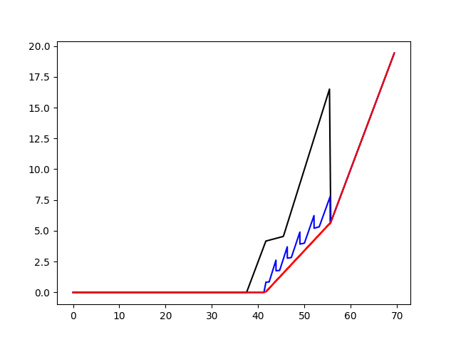
A graphic illustration of VT−1∗,n/nsuperscriptsubscript𝑉𝑇1𝑛𝑛V_{T-1}^{*,n}/n as a function of ST−1subscript𝑆𝑇1S_{T-1} is given in Figure 1.

Refer to caption
Figure 1: The function x=ST−1↦g​(T−1,x,n)/n=VT−1∗,n/n𝑥subscript𝑆𝑇1maps-to𝑔𝑇1𝑥𝑛𝑛superscriptsubscript𝑉𝑇1𝑛𝑛x=S_{T-1}\mapsto g(T-1,x,n)/n=V_{T-1}^{*,n}/n, K=500𝐾500K=500, for n=1𝑛1n=1 (black), n=5𝑛5n=5 (blue), n=100𝑛100n=100 (red).

We observe that VT−1∗,nsuperscriptsubscript𝑉𝑇1𝑛V_{T-1}^{*,n} is not a convex function of ST−1subscript𝑆𝑇1S_{T-1} even if the payoff function is and, moreover, g​(T−1,x,n)≠n​g​(T−1,x,1)𝑔𝑇1𝑥𝑛𝑛𝑔𝑇1𝑥1g(T-1,x,n)\neq ng(T-1,x,1).

4 Numerical illustration

In this section, we illustrate the method developed above when the underlying asset S𝑆S is the french CAC 40 index and the European claim is the Call option. The historical data is composed of daily observations of the CAC 40 values between the 6th of June 2019 and the 16th of June 2021. We use the two first years of the data set to calibrate the model while we implement the model on the third year. Here, we suppose that suppℱt⁡St+1=[ktd​St,ktu​St]subscriptsuppsubscriptℱ𝑡subscript𝑆𝑡1subscriptsuperscript𝑘𝑑𝑡subscript𝑆𝑡subscriptsuperscript𝑘𝑢𝑡subscript𝑆𝑡\operatorname{supp}_{{\cal F}_{t}}S_{t+1}=[k^{d}_{t}S_{t},k^{u}_{t}S_{t}] where ktdsubscriptsuperscript𝑘𝑑𝑡k^{d}_{t} and ktusubscriptsuperscript𝑘𝑢𝑡k^{u}_{t} are estimated as follows:

ktdsubscriptsuperscript𝑘𝑑𝑡\displaystyle k^{d}_{t} =\displaystyle= mini=j,⋯,N⁡St+1(j)/St(j),subscript𝑖𝑗⋯𝑁superscriptsubscript𝑆𝑡1𝑗superscriptsubscript𝑆𝑡𝑗\displaystyle\min_{i=j,\cdots,N}S_{t+1}^{(j)}/S_{t}^{(j)},
ktusubscriptsuperscript𝑘𝑢𝑡\displaystyle k^{u}_{t} =\displaystyle= maxi=j,⋯,N⁡St+1(j)/St(j),subscript𝑖𝑗⋯𝑁superscriptsubscript𝑆𝑡1𝑗superscriptsubscript𝑆𝑡𝑗\displaystyle\max_{i=j,\cdots,N}S_{t+1}^{(j)}/S_{t}^{(j)},

where N𝑁N is the number of training periods and St(j)superscriptsubscript𝑆𝑡𝑗S_{t}^{(j)} are the observed values at time t𝑡t during the j-th periods. The algorithms are written in Python. The main difficulty is to write a code whose execution time is reasonable. Indeed, recall that the price function g​(t,x)𝑔𝑡𝑥g(t,x) is computed backwardly from g​(t+1,x)𝑔𝑡1𝑥g(t+1,x). If this function g​(t,x)𝑔𝑡𝑥g(t,x) is naively coded from g​(t+1,x)𝑔𝑡1𝑥g(t+1,x), then the computation may take more than two weeks ! So it is better to approximate, at each step, the function g​(t,x)𝑔𝑡𝑥g(t,x) as a numpy array consisting of discretized values following a grid (xi)i=0Ntsuperscriptsubscriptsubscript𝑥𝑖𝑖0subscript𝑁𝑡(x_{i})_{i=0}^{N_{t}} where xi=s​t​e​p∗isubscript𝑥𝑖𝑠𝑡𝑒𝑝𝑖x_{i}=step*i. Here, we choose s​t​e​p=0.1𝑠𝑡𝑒𝑝0.1step=0.1 and Ntsubscript𝑁𝑡N_{t} is chosen so that xN0≤S0maxsubscript𝑥subscript𝑁0superscriptsubscript𝑆0maxx_{N_{0}}\leq S_{0}^{{\rm max}} where S0maxsuperscriptsubscript𝑆0maxS_{0}^{{\rm max}} is the maximal value for S0subscript𝑆0S_{0} that we observe in our data. At last, xNt≤S0max∗(maxr≤t⁡kru)tsubscript𝑥subscript𝑁𝑡superscriptsubscript𝑆0maxsuperscriptsubscript𝑟𝑡subscriptsuperscript𝑘𝑢𝑟𝑡x_{N_{t}}\leq S_{0}^{{\rm max}}*(\max_{r\leq t}k^{u}_{r})^{t}.

The relative hedging error is defined as ϵT=100∗(VT−g​(T,ST))/STsubscriptitalic-ϵ𝑇100subscript𝑉𝑇𝑔𝑇subscript𝑆𝑇subscript𝑆𝑇\epsilon_{T}=100*(V_{T}-g(T,S_{T}))/S_{T} where (Vt∗)t=0,⋯,Tsubscriptsuperscriptsubscript𝑉𝑡𝑡0⋯𝑇(V_{t}^{*})_{t=0,\cdots,T} is the optimal super-hedging portfolio process whose initial value is the minimal super-hedging price, as computed in the last section. We present in Figure 2.1 the distribution of ϵTsubscriptitalic-ϵ𝑇\epsilon_{T} when n=1𝑛1n=1. Of course, we expect that ϵT≥0subscriptitalic-ϵ𝑇0\epsilon_{T}\geq 0 a.s. and this is confirmed on our test data set. Note that, we could have observed some negative values as the model is calibrated from data values anterior to the test data set.

Refer to caption
Refer to caption
Figure 2: F2.1: Super-hedging errors with n=1𝑛1n=1 and K=3000𝐾3000K=3000. F2.2: Comparison of the optimal strategies per unit of claims for n=1𝑛1n=1 and n=10𝑛10n=10.

Let us denote by g​(t,x,n)𝑔𝑡𝑥𝑛g(t,x,n) the price function at time t𝑡t of the optimal portfolio process, i.e. Vt∗,n=g​(t,St,n)superscriptsubscript𝑉𝑡𝑛𝑔𝑡subscript𝑆𝑡𝑛V_{t}^{*,n}=g(t,S_{t},n) such that VT∗,n≥ξTnsuperscriptsubscript𝑉𝑇𝑛superscriptsubscript𝜉𝑇𝑛V_{T}^{*,n}\geq\xi_{T}^{n} a.s., when the European claim is ξTn:=n∗(ST−K)+assignsuperscriptsubscript𝜉𝑇𝑛𝑛superscriptsubscript𝑆𝑇𝐾\xi_{T}^{n}:=n*(S_{T}-K)^{+}. The natural question is the following: Do we have g​(t,x,n)=n​g​(t,x,1)𝑔𝑡𝑥𝑛𝑛𝑔𝑡𝑥1g(t,x,n)=ng(t,x,1) ? The answer is yes when real-valued strategies are allowed since the hedging problem is then linear with respect to the number of claims.

In the case of integer-valued strategies, the answer is not trivial. It is actually negative, see the first example above. By definition of the infimum super-hedging price, we have g​(t,x,n)≤n​g​(t,x,1)𝑔𝑡𝑥𝑛𝑛𝑔𝑡𝑥1g(t,x,n)\leq ng(t,x,1). As a first step, we have computed the relative infimum super-hedging prices per unit of claims, i.e. V0∗,n/nsuperscriptsubscript𝑉0𝑛𝑛V_{0}^{*,n}/n at time 00, for different values of n𝑛n on each period of the test data set. Then, computing the average of the V0∗,n/nsuperscriptsubscript𝑉0𝑛𝑛V_{0}^{*,n}/n values over all the periods, we get that the empirical average of V0∗,n/nsuperscriptsubscript𝑉0𝑛𝑛V_{0}^{*,n}/n is approximately equal to 49.48%percent49.4849.48\% for n=1,5,10,15,20𝑛15101520n=1,5,10,15,20. Nevertheless, we observe that the price function per unit of unit of claims, i.e. g​(0,S0,n)/n𝑔0subscript𝑆0𝑛𝑛g(0,S_{0},n)/n is non-increasing when n𝑛n increases, see Figure 3. This implies that the equality g​(t,x,n)=n​g​(t,x,1)𝑔𝑡𝑥𝑛𝑛𝑔𝑡𝑥1g(t,x,n)=ng(t,x,1) does not hold. In Figure 3, we clearly observe the convergence of x↦g​(0,x,n)/nmaps-to𝑥𝑔0𝑥𝑛𝑛x\mapsto g(0,x,n)/n as n→∞→𝑛n\to\infty.

The same question arises for the optimal strategy associated to V∗,nsuperscript𝑉𝑛V^{*,n}, i.e. do we have θ∗​(t,St,n)=n​θ∗​(t,St,1)superscript𝜃𝑡subscript𝑆𝑡𝑛𝑛superscript𝜃𝑡subscript𝑆𝑡1\theta^{*}(t,S_{t},n)=n\theta^{*}(t,S_{t},1)? Intuitively, this is a priori not the case as θ∗​(t,St,1)=θ∗​(t,St,n)/nsuperscript𝜃𝑡subscript𝑆𝑡1superscript𝜃𝑡subscript𝑆𝑡𝑛𝑛\theta^{*}(t,S_{t},1)=\theta^{*}(t,S_{t},n)/n could be not integer-valued. This is confirmed at time 00 when we compute the optimal strategy θ∗​(0,S0,n)/nsuperscript𝜃0subscript𝑆0𝑛𝑛\theta^{*}(0,S_{0},n)/n per unit of claims. This is illustrated by Figure 2.2 where we compare θ∗​(0,S0,n)/nsuperscript𝜃0subscript𝑆0𝑛𝑛\theta^{*}(0,S_{0},n)/n for n=10𝑛10n=10 to θ∗​(0,S0,1)superscript𝜃0subscript𝑆01\theta^{*}(0,S_{0},1). We may observe that the optimal strategy per unit of claims θ∗​(0,S0,n)/nsuperscript𝜃0subscript𝑆0𝑛𝑛\theta^{*}(0,S_{0},n)/n (blue graph) is smaller that θ∗​(0,S0,1)superscript𝜃0subscript𝑆01\theta^{*}(0,S_{0},1) for n=10𝑛10n=10.

Refer to caption
Figure 3: Super-hedging price mapping x↦g​(0,x,n)/nmaps-to𝑥𝑔0𝑥𝑛𝑛x\mapsto g(0,x,n)/n of n𝑛n units of call option per unit of claims for different values of n=1𝑛1n=1 (black), n=3𝑛3n=3 (grey), n=5𝑛5n=5 (green), n=7𝑛7n=7 (blue), n=10𝑛10n=10 (orange), n=100𝑛100n=100 (red).

References

  • [1] Baptiste J., Carassus L. and Lépinette E. Pricing without martingale measures. Preprint. https://hal.archives-ouvertes.fr/hal-01774150.
  • [2] Bienstock D. Computational study of a family of mixed-integer quadratic programming problems. Math. Programming, 74, 121–140, 1996.
  • [3] Bonami P. and Lejeune M. A. An exact solution approach for portfolio optimization problems under stochastic and integer constraints. Oper. Res., 57, 650–670, 2009.
  • [4] Black F. and Scholes M. The pricing of options and corporate liabilities. Journal of Political Economy, 81, 3, 637-659, 1973.
  • [5] Baumann P. and Trautmann N. Portfolio-optimization models for small investors. Math. Methods Oper. Res., 77, pp. 345–356, 2013.
  • [6] Carassus L. and Lépinette E. Pricing without no-arbitrage condition in discrete-time. Journal of Mathematical Analysis and Applications, 505, 1, 125441, 2022.
  • [7] Deng X., Li Z. and Wang S. Computational complexity of arbitrage in frictional security market. International Journal of Foundations of Computer Science, 13, 681–684, 2002.
  • [8] Dalang E.C., Morton A. and Willinger W. Equivalent martingale measures and no-arbitrage in stochastic securities market models. Stochastics and Stochastic Reports, 29, 185-201, 1990.
  • [9] Delbaen F. and Schachermayer W. A general version of the fundamental theorem of asset pricing. Mathematische Annalen, 300, 463-520, 1994.
  • [10] Delbaen F. and Schachermayer W. The fundamental theorem of asset pricing for unbounded stochastic processes. Mathematische Annalen, 312, 215-250, 1996.
  • [11] Delbaen F. and Schachermayer W. The mathematics of arbitrage. Springer Finance, Ed. 2006, 2nd printing, XVI, 2008.
  • [12] Gerhold S. and Krühner P. Dynamic trading under trading constraints. Finance and Stochastics, 22, 919-957, 2018.
  • [13] El Mansour Meriem and Lépinette E. Conditional interior and conditional closure of a random sets). Journal of Optimization Theory and Applications, 5051 187, 356-369, 2020.