\institution

Lab-Sticc, ENSTA-Bretagne

Inertial control of a spinning flat disk

Luc Jaulin

Abstract. This paper proposes a Lyapunov based approach to control the rotation of a flat disk spinning in the space without external forces. The motion of the disk is governed by the Euler’s rotation equation for spinning objects. The control is made through the inertia matrix of the disk.

1 Spinning disk

Consider a disk spinning in the space without any gravity. The disk is assumed to be flat, i.e., its inertia matrix [9]

\mathbf{I}=\left(\begin{array}[]{ccc}I_{1}&0&0\\ 0&I_{2}&0\\ 0&0&I_{3}\end{array}\right)

(1)

should satisfy

•

the positivity condition: $I_{1}>0,I_{2}>0,I_{3}>0$ ;
•

the flatness condition: $I_{1}=I_{2}+I_{3}$ .

We assume that we can control the inertia matrix via some internal forces in a strap down manner. It means that we have no inertial wheels. Instead, we could slightly modify $\mathbf{I}$ by dilatation or compression of some parts of the disk. We also consider that we are not able to change the center of gravity of the disk.

At rest, the inertial matrix is assumed to be

\bar{\mathbf{I}}=\left(\begin{array}[]{ccc}\bar{I}_{1}&0&0\\ 0&\bar{I}_{2}&0\\ 0&0&\bar{I}_{3}\end{array}\right)=\left(\begin{array}[]{ccc}\frac{1}{2}mr^{2}&0&0\\ 0&\frac{1}{4}mr^{2}&0\\ 0&0&\frac{1}{4}mr^{2}\end{array}\right)

(2)

where $r$ is the radius of the disk and $m$ is its mass. The entries of the inertia matrix can change as soon as the positivity and the flatness conditions are satisfied. Equivalently, and for a better visualization, we may assume that, we have two symmetric pairs of masses which can move along the $y$ and $z$ axis (see Figure 1).

Refer to caption — Figure 1: The disk spins and the two pairs of masses (black and green) can slightly move in order the control the motion of the rotation vector $\boldsymbol{\omega}$

The inertia of the disk is now

\mathbf{I}=\left(\begin{array}[]{ccc}\frac{1}{2}mr^{2}+\text{$\frac{1}{2}$$\ell_{2}^{2}+\frac{1}{2}\ell_{3}^{2}$}&0&0\\ 0&\frac{1}{4}mr^{2}+\text{$\text{$\frac{1}{2}$$\ell_{3}^{2}$}$}&0\\ 0&0&\frac{1}{4}mr^{2}+\text{$\frac{1}{2}$$\text{$\ell_{2}^{2}$}$}\end{array}\right)

(3)

where $\ell_{2}$ corresponds to the distance of the $y$ -masses (green) to the center and $\ell_{3}$ is the distance of the $z$ -masses (black) to the center. Our objective is to propose a controller to modify the rotation of the disk. The control objective is not so clear at the moment since rotation cannot be controlled arbitrarily. Indeed, the angular momentum remains constant and is thus non controllable.

This paper is organized as follows. Section 2 gives the state equations of the spinning disk. Section 3 proposes different controllers to change behavior of the rotation of the disk. Section 4 concludes the paper.

2 State equation of the flat disk

The state equations are obtained from the conservation of angular momentum. If $\mathbf{R}$ defines the orientation matrix of a rigid body (for us the flat disk), then the angular momentum is

\mathcal{L}=\mathbf{R}\mathbf{I}\boldsymbol{\omega}_{r}

(4)

where $\boldsymbol{\omega}_{r}$ is the rotation vector of the body expressed in its own frame.

Since it is constant, we have

\begin{array}[]{cl}&\dot{\mathbf{R}}\mathbf{I}\boldsymbol{\omega}_{r}+\mathbf{R}\dot{\mathbf{\cdot I}\cdot}\boldsymbol{\omega}_{r}+\mathbf{R}\cdot\mathbf{I}\cdot\dot{\boldsymbol{\omega}}_{r}=\mathbf{0}\\ \Leftrightarrow&\mathbf{R}^{\text{T}}\dot{\mathbf{R}}\mathbf{I}\boldsymbol{\omega}_{r}+\dot{\mathbf{I}}\cdot\boldsymbol{\omega}_{r}+\mathbf{I}\cdot\dot{\boldsymbol{\omega}}_{r}=\mathbf{0}\end{array}

(5)

We get the Euler’s rotation equation

\dot{\boldsymbol{\omega}}_{r}=\mathbf{I}^{-1}\cdot\left(-\dot{\mathbf{I}}\cdot\boldsymbol{\omega}_{r}-\boldsymbol{\omega}_{r}\wedge\mathbf{I}\cdot\boldsymbol{\omega}_{r}\right)

(6)

If we include the orientation, we have the motion equation

\left\{\begin{array}[]{cclcl}\mathbf{\dot{R}}&&=&&\mathbf{R}\cdot\textnormal{(}\boldsymbol{\omega}_{r}\wedge\textnormal{)}\\ \dot{\boldsymbol{\omega}}_{r}&&=&&\mathbf{I}^{-1}\cdot\left(-\dot{\mathbf{I}}\cdot\boldsymbol{\omega}_{r}-\boldsymbol{\omega}_{r}\wedge\mathbf{I}\cdot\boldsymbol{\omega}_{r}\right)\end{array}\right.

(7)

which will be used for the simulation. For the control we do not want to control the orientation $\mathbf{R}$ ; we only want to control $\boldsymbol{\omega}_{r}$ . In what follows, the component of $\boldsymbol{\omega}_{r}$ will be denoted by $\omega_{1},\omega_{2},\omega_{3}$ , i.e., we will write

\boldsymbol{\omega}_{r}=(\omega_{1},\omega_{2},\omega_{3})^{\text{T}}.

(8)

Since $\mathbf{I}$ is diagonal, the time-varying Euler equation rewrites into

\left\{\begin{array}[]{ccc}I_{1}\dot{\omega}_{1}&=&-\dot{I}_{1}\omega_{1}-(I_{3}-I_{2})\omega_{2}\omega_{3}\\ I_{2}\dot{\omega}_{2}&=&-\dot{I}_{2}\omega_{2}-(I_{1}-I_{3})\omega_{3}\omega_{1}\\ I_{3}\dot{\omega}_{3}&=&-\dot{I}_{3}\omega_{3}-(I_{2}-I_{1})\omega_{1}\omega_{2}\end{array}\right.

(9)

From (3), we have

\begin{array}[]{ccc}I_{1}&=&\frac{1}{2}mr^{2}+\frac{1}{2}\ell_{2}^{2}+\frac{1}{2}\ell_{3}^{2}\\ I_{2}&=&\frac{1}{4}mr^{2}+\frac{1}{2}\ell_{2}^{2}\\ I_{3}&=&\frac{1}{4}mr^{2}+\frac{1}{2}\ell_{3}^{2}\end{array}

(10)

where we assumed that the sum of the control masses along the $y$ axis are equal to $1$ . The same assumption is taken for the masses along the $z$ axis. We have

\begin{array}[]{ccc}\dot{I}_{1}&=&\ell_{2}\dot{\ell}_{2}+\ell_{3}\dot{\ell}_{3}\\ \dot{I}_{2}&=&\ell_{2}\dot{\ell}_{2}\\ \dot{I}_{3}&=&\ell_{3}\dot{\ell}_{3}\end{array}

(11)

The state equations of the system are thus

\left\{\begin{array}[]{ccc}\dot{\omega}_{1}&=&-\frac{\omega_{1}}{I_{2}+I_{3}}(\ell_{2}\dot{\ell}_{2}+\ell_{3}\dot{\ell}_{3})-\frac{I_{3}-I_{2}}{I_{2}+I_{3}}\omega_{2}\omega_{3}\\ \dot{\omega}_{2}&=&-\frac{\omega_{2}}{I_{2}}\ell_{2}\dot{\ell}_{2}-\omega_{3}\omega_{1}\\ \dot{\omega}_{3}&=&-\frac{\omega_{3}}{I_{3}}\ell_{3}\dot{\ell}_{3}+\omega_{1}\omega_{2}\\ \dot{I}_{2}&=&\ell_{2}\dot{\ell}_{2}\\ \dot{I}_{3}&=&\ell_{3}\dot{\ell}_{3}\end{array}\right.

(12)

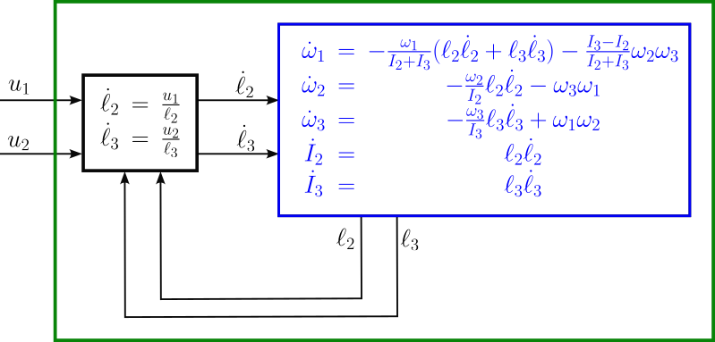
A first simplification of the control problem can be obtained by adding the following controller

\left\{\begin{array}[]{ccc}\dot{\ell}_{2}&=&\frac{u_{1}}{\ell_{2}}\\ \dot{\ell}_{3}&=&\frac{u_{2}}{\ell_{3}}\end{array}\right.

(13)

where $u_{1},u_{2}$ are some intermediate input (see Figure 2), we get the state equations for the flat disk:

\left\{\begin{array}[]{ccc}\dot{\omega}_{1}&=&-\frac{\omega_{1}}{I_{2}+I_{3}}(u_{1}+u_{2})-\frac{I_{3}-I_{2}}{I_{2}+I_{3}}\omega_{2}\omega_{3}\\ \dot{\omega}_{2}&=&-\frac{\omega_{2}}{I_{2}}u_{1}-\omega_{3}\omega_{1}\\ \dot{\omega}_{3}&=&-\frac{\omega_{3}}{I_{3}}u_{2}+\omega_{1}\omega_{2}\\ \dot{I}_{2}&=&u_{1}\\ \dot{I}_{3}&=&u_{2}\end{array}\right.

(14)

The state vector is $\mathbf{x}=(\omega_{1},\omega_{2},\omega_{3},I_{2},I_{3})$ and the input vector is $\mathbf{u}=(u_{1},u_{2})$ .

3 Controller

This section proposes different controllers to change the spinning behavior of the flat disk. The principle is to combine Lyapunov control theory in the context of rotating object [6].

3.1 Principle

To find a controller for our system (14), we follow a Lyapunov control approach [8], [5]. For this, we choose a positive function $V(\mathbf{x})$ , namely the objective function, such that $V(\mathbf{x})=0$ when the objective is reached.

Let us rewrite the state equation into an affine form [4]:

\underset{=\dot{\mathbf{x}}}{\underbrace{\left(\begin{array}[]{c}\dot{\omega}_{1}\\ \dot{\omega}_{2}\\ \dot{\omega}_{3}\\ \dot{I}_{2}\\ \dot{I}_{3}\end{array}\right)}}=\underset{=\mathbf{f}(\mathbf{x})}{\underbrace{\left(\begin{array}[]{c}-\frac{I_{3}-I_{2}}{I_{2}+I_{3}}\omega_{2}\omega_{3}\\ -\omega_{3}\omega_{1}\\ \omega_{1}\omega_{2}\\ 0\\ 0\end{array}\right)}}+\underset{=\mathbf{g}_{1}(\mathbf{x})}{\underbrace{\left(\begin{array}[]{c}-\frac{\omega_{1}}{I_{2}+I_{3}}\\ -\frac{\omega_{2}}{I_{2}}\\ 0\\ 1\\ 0\end{array}\right)}}\cdot u_{1}+\underset{=\mathbf{g}_{2}(\mathbf{x})}{\underbrace{\left(\begin{array}[]{c}-\frac{\omega_{1}}{I_{2}+I_{3}}\\ 0\\ -\frac{\omega_{3}}{I_{3}}\\ 0\\ 1\end{array}\right)}}\cdot u_{2}.

(15)

The time derivative of $V$ is

\dot{V}(\mathbf{x},\mathbf{u})=\mathcal{L}_{\mathbf{f}}V(\mathbf{x})+\mathcal{L}_{\mathbf{g}_{1}}V(\mathbf{x})\cdot u_{1}+\mathcal{L}_{\mathbf{g}_{2}}V(\mathbf{x})\cdot u_{2},

(16)

where $\mathcal{L}$ is the Lie derivative operator. Since the solution of

\begin{array}[]{cc}\min&a_{1}u_{1}+a_{2}u_{2}\\ \text{s.t.}&u_{1}^{2}+u_{2}^{2}=1\end{array}

(17)

where $\,a_{1}=\mathcal{L}_{\mathbf{g}_{1}}V(\mathbf{x}),\,a_{2}=\mathcal{L}_{\mathbf{g}_{2}}V(\mathbf{x})$ , is

\left(\begin{array}[]{c}u_{1}\\ u_{2}\end{array}\right)=-\frac{1}{\sqrt{a_{1}^{2}+a_{2}^{2}}}\cdot\left(\begin{array}[]{c}a_{1}\\ a_{2}\end{array}\right),

(18)

we conclude that a Lyapunov like controller to reach our objective is

\mathbf{u}=-\frac{1}{\sqrt{(\mathcal{L}_{\mathbf{g}_{1}}V(\mathbf{x}))^{2}+(\mathcal{L}_{\mathbf{g}_{2}}V(\mathbf{x}))^{2}}}\cdot\left(\begin{array}[]{c}\mathcal{L}_{\mathbf{g}_{1}}V(\mathbf{x})\\ \mathcal{L}_{\mathbf{g}_{2}}V(\mathbf{x})\end{array}\right).

(19)

3.2 Alignment controller

Assume that we want the disk spins around one principal axis of the body. For instance its first axis, i.e., the $x$ -axis. We define the objective function

V(\mathbf{x})=\frac{1}{2}\left(\omega_{2}^{2}+\omega_{3}^{2}+(I_{2}-\bar{I}_{2})^{2}+(I_{3}-\bar{I}_{3})^{2}\right).

(20)

The quantity $\omega_{2}^{2}+\omega_{3}^{2}$ corresponds to the alignment error. Note that when $V(\mathbf{x})=0$ , we have $\omega_{2}=\omega$ ${}_{3}=0$ (the alignment is performed) and $\mathbf{I}=\bar{\mathbf{I}}$ (the inertia matrix is at its nominal position). The time derivative of $V$ is

\begin{array}[]{ccl}\dot{V}(\mathbf{x})&=&\omega_{2}\dot{\omega}_{2}+\omega_{3}\dot{\omega}_{3}+(I_{2}-\bar{I}_{2})\dot{I}_{2}+(I_{3}-\bar{I}_{3})\dot{I}_{3}\\ &=&\omega_{2}\left(-\frac{\omega_{2}}{I_{2}}u_{1}-\omega_{3}\omega_{1}\right)+\omega_{3}\left(-\frac{\omega_{3}}{I_{3}}u_{2}+\omega_{1}\omega_{2}\right)+(I_{2}-\bar{I}_{2})u_{1}+(I_{3}-\bar{I}_{3})u_{2}\\ &=&-\frac{\omega_{2}^{2}}{I_{2}}u_{1}-\omega_{3}\omega_{1}\omega_{2}-\frac{\omega_{3}^{2}}{I_{3}}u_{2}+\omega_{1}\omega_{2}\omega_{3}+(I_{2}-\bar{I}_{2})u_{1}+(I_{3}-\bar{I}_{3})u_{2}\\ &=&\underset{\mathcal{L}_{\mathbf{f}}V}{\underbrace{0\cdot\omega_{1}\omega_{2}\omega_{3}}}+\underset{\mathcal{L}_{\mathbf{g}_{1}}V}{\underbrace{\left(-\frac{\omega_{2}^{2}}{I_{2}}+(I_{2}-\bar{I}_{2})\right)}}\cdot u_{1}+\underset{\mathcal{L}_{\mathbf{g}_{2}}V}{\underbrace{\left(-\frac{\omega_{3}^{2}}{I_{3}}+(I_{3}-\bar{I}_{3})\right)}}\cdot u_{2}\end{array}

(21)

The same result would have easily been obtained using a symbolic calculus module such as Sympy which is an open source computer algebra system written in Python. The corresponding Sympy script is the following

from sympy import*
from sympy.diffgeom import*
C=CoordSystem(’C’,Patch(’P’,Manifold(’M’,5)),{[w1,w2,w3,I2,I3]})
w1,w2,w3,I2,I3 = C.coord\_functions()
E = C.base\_vectors()
F=-((I3-I2)/(I2+I3))*w2*w3*E[0]+-w3*w1*E[1]+w1*w2*E[2]
G1=-(w1/(I2+I3))*E[0]-(w2/I2)*E[1]+E[3]
G2=-(w1/(I2+I3))*E[0]-(w3/I3)*E[2]+E[4]
V = 1/2*w2**2 + 1/2*w3**2 + 1/2*(I2-I20)**2 + 1/2*(I3-I30)**2
LfV=LieDerivative(F,V)
Lg1V=LieDerivative(G1,V)
Lg2V=LieDerivative(G2,V)

Stability analysis. With our controller, we have $\dot{V}(\mathbf{x})=0$ if

\left\{\begin{array}[]{ccc}-\frac{\omega_{2}^{2}}{I_{2}}+I_{2}-\bar{I}_{2}&=&0\\ -\frac{\omega_{3}^{2}}{I_{3}}+I_{3}-\bar{I}_{3}&=&0\end{array}\right.

(22)

We conclude that it it possible to converge to values $\bar{\omega}_{1},\bar{\omega}_{2},\bar{\omega}_{3}$ that do not correspond to the desired alignment. Equivalently, we may have $\bar{\omega}_{2}\neq 0,$ or $\bar{\omega}_{3}\neq 0$ .

Figure 3 illustrates the behavior of the controller. The initial rotation vector is $\boldsymbol{\omega}(0)=(10^{-5},10,0).$ The first subfigure (top-left) shows the kinetic energy $E_{K}$ of the disk (blue) and the objective function $V(t)$ (red) with respect to $t$ for $t\in[0,40]$ . The second subfigure (top right) shows the evolution of the components of $\boldsymbol{\omega}$ in the frame box $[0,40]\times[-7,10].$ The third subfigure represents the evolution of the vector $(\omega_{2},\omega_{3}).$ The frame box is $[-5,5]\times[-5,5]$ . The last subfigure represents the component $I_{2},I_{3}$ of the inertia matrix in the frame box $[-0.2,2.5]\times[-0.2,2]$ . Since the controller is not able to cancel $(\omega_{2},\omega_{3})$ , we consider that the alignment objective is only partially reach.

The strategy followed by the controller is first to increase $I_{2}$ to make the second axis the intermediate axis (see the $4$ th Subfigure). As a consequence, due to instability of the second axis, also known as the Dzhanibekov effect (even if first shown by Poinsot [7]), the component $\omega_{2}$ of $\boldsymbol{\omega}$ is able to decrease without precession (see the $3$ th Subfigure). Then in a second step, the control changes its strategy to generate an oscillation between $I_{2}$ and $I_{3}$ . This yields a convergence of $\omega_{1}$ , the rotation along the first axis. We also observe that $\omega_{2}$ and $\omega_{3}$ do not converge to a static value.

3.3 Passive controller

We now want the disk losses energy with the intuition that it may limit the precession. Another motivation is that it may help to find an objective function which could help to guaranty the stability. A passivity control approach can be used for this purpose [3][1]. We define the mechanical energy as

\begin{array}[]{ccc}V(\mathbf{x})&=&\frac{1}{2}I_{1}\omega_{1}^{2}+\frac{1}{2}I_{2}\omega_{2}^{2}+\frac{1}{2}I_{3}\omega_{3}^{2}+\frac{1}{2}(I_{2}-\bar{I}_{2})^{2}+\frac{1}{2}(I_{3}-\bar{I}_{3})^{2}\end{array}.

(23)

The quantity $\frac{1}{2}\boldsymbol{\omega}_{r}^{\text{T}}\mathbf{I}\boldsymbol{\omega}_{r}$ corresponds to kinetic energy and $\frac{1}{2}(I_{2}-\bar{I}_{2})^{2}+\frac{1}{2}(I_{3}-\bar{I}_{3})^{2}$ is the artificial potential energy.

We have

\begin{array}[]{ccl}\dot{V}(\mathbf{x})&=&I_{1}\omega_{1}\dot{\omega}_{1}+I_{2}\omega_{2}\dot{\omega}_{2}+I_{3}\omega_{3}\dot{\omega}_{3}+\frac{1}{2}\omega_{1}^{2}\dot{I}_{1}+\frac{1}{2}\omega_{2}^{2}\dot{I}_{2}+\frac{1}{2}\omega_{3}^{2}\dot{I}_{3}\\ &&+(I_{2}-\bar{I}_{2})\dot{I}_{2}+(I_{3}-\bar{I}_{3})\dot{I}_{3}\\ &=&\left(I_{2}+I_{3}\right)\omega_{1}\left(-\frac{\omega_{1}}{I_{2}+I_{3}}(u_{1}+u_{2})-\frac{I_{3}-I_{2}}{I_{2}+I_{3}}\omega_{2}\omega_{3}\right)\\ &&+I_{2}\omega_{2}\left(-\frac{\omega_{2}}{I_{2}}u_{1}-\omega_{3}\omega_{1}\right)+I_{3}\omega_{3}\left(-\frac{\omega_{3}}{I_{3}}u_{2}+\omega_{1}\omega_{2}\right)\\ &&+\frac{1}{2}\omega_{1}^{2}(u_{1}+u_{2})+\frac{1}{2}\omega_{2}^{2}u_{1}+\frac{1}{2}\omega_{3}^{2}u_{2}+(I_{2}-\bar{I}_{2})u_{1}+(I_{3}-\bar{I}_{3})u_{2}\\ &=&-\frac{1}{2}\omega_{1}^{2}u_{1}-\frac{1}{2}\omega_{2}^{2}u_{1}-\frac{1}{2}\omega_{1}^{2}u_{2}-\frac{1}{2}\omega_{3}^{2}u_{2}+(I_{2}-\bar{I}_{2})u_{1}+(I_{3}-\bar{I}_{3})u_{2}\\ &=&\underset{\mathcal{L}_{\mathbf{f}}V}{\underbrace{0}}+\underset{\mathcal{L}_{\mathbf{g}_{1}}V}{\underbrace{\left(-\frac{1}{2}\omega_{1}^{2}-\frac{1}{2}\omega_{2}^{2}+I_{2}-\bar{I}_{2}\right)}}\cdot u_{1}+\underset{\mathcal{L}_{\mathbf{g}_{2}}V}{\underbrace{\left(-\frac{1}{2}\omega_{1}^{2}-\frac{1}{2}\omega_{3}^{2}+I_{3}-\bar{I}_{3}\right)}}\cdot u_{2}\end{array}

The same result is obtained using Sympy taking

V = 1/2*(I2+I3)*w1**2+ 1/2*I2*w2**2 + 1/2*I3*w3**2
    + 1/2*(I2-I20)**2 + 1/2*(I3-I30)**2

Figure 4 illustrates the behavior of the controller for $t\in[0,40]$ . The initial rotation vector is $\boldsymbol{\omega}(0)=(10,4,1).$ The meaning of the plots are those given for Figure 3. The frame for the subfigures are $[0,40]\times[0,1]$ , $[0,40]\times[-5,10],$ $[-5,5]\times[-5,5]$ and $[-0.2,6]\times[-0.2,6]$ , respectively. We observe that the passivity approach for the flat disk is not sufficient to cancel the precession.

3.4 Precession controller

To cancel the precession, we define the objective function

\begin{array}[]{ccc}V(\mathbf{x})&=&\frac{1}{2}\left((I_{3}-I_{2})\omega_{2}\omega_{3}\right)^{2}+\frac{1}{2}\left((I_{1}-I_{3})\omega_{3}\omega_{1}\right)^{2}+\frac{1}{2}\left((I_{2}-I_{1})\omega_{1}\omega_{2}\right)^{2}\\ &&+\frac{1}{2}(I_{2}-\bar{I}_{2})^{2}+\frac{1}{2}(I_{3}-\bar{I}_{3})^{2}.\end{array}

(24)

The quantity

\left((I_{3}-I_{2})\omega_{2}\omega_{3}\right)^{2}+\left((I_{1}-I_{3})\omega_{3}\omega_{1}\right)^{2}+\left((I_{2}-I_{1})\omega_{1}\omega_{2}\right)^{2}=\|\boldsymbol{\omega}_{r}\wedge\mathbf{I}\cdot\boldsymbol{\omega}_{r}\|^{2}

(25)

can be interpreted precession energy, i.e., a part of the kinetic energy that creates the precession and that can be recovered. Indeed, when $\boldsymbol{\omega}_{r}\wedge\mathbf{I}\cdot\boldsymbol{\omega}_{r}=\mathbf{0}$ , we see from the Euler equation that $\dot{\boldsymbol{\omega}}_{r}=\mathbf{0}$ when $\mathbf{u}=\mathbf{0},$ which means that we have no more precession.

Using Sympy with

V = 1/2*((I3-I2)*w2*w3)**2 + 1/2*((I2)*w1*w3)**2
     + 1/2*((-I3)*w1*w2)**2
     + 1/2*(I2-I20)**2 + 1/2*(I3-I30)**2

we get

\begin{array}[]{ccc}\mathcal{L}_{\mathbf{f}}V(\mathbf{x})&=&\frac{\left(\left(\omega_{2}^{2}I_{3}^{2}+\omega_{3}^{2}I_{2}^{2}\right)\left(I_{2}-I_{3}\right)+\left(I_{2}+I_{3}\right)\left(\left(I_{2}-I_{3}\right)^{2}\omega_{2}^{2}-\left(I_{2}-I_{3}\right)^{2}\omega_{3}^{2}+\omega_{1}^{2}I_{2}^{2}-\omega_{1}^{2}I_{3}^{2}\right)\right)\omega_{1}\omega_{2}\omega_{3}}{I_{2}+I_{3}}\\ \mathcal{L}_{\mathbf{g}_{1}}V(\mathbf{x})&=&\frac{1-\left(\left(I_{2}-I_{3}\right)^{2}\omega_{3}^{2}+\omega_{1}^{2}I_{3}^{2}\right)\omega_{2}^{2}}{I_{2}}-\frac{\left(\omega_{2}^{2}I_{3}^{2}+\omega_{3}^{2}I_{2}^{2}\right)\omega_{1}^{2}}{I_{2}+I_{3}}+\frac{\left(I_{2}-\bar{I}_{2}\right)+\left(I_{2}-I_{3}\right)\omega_{2}^{2}\omega_{3}^{2}+\omega_{1}^{2}\omega_{3}^{2}I_{2}}{I_{2}+I_{3}}\\ \mathcal{L}_{\mathbf{g}_{2}}V(\mathbf{x})&=&\frac{1-\left(\left(I_{2}-I_{3}\right)^{2}\omega_{2}^{2}+\omega_{1}^{2}I_{2}^{2}\right)\omega_{3}^{2}}{I_{3}}-\frac{\left(\omega_{2}^{2}I_{3}^{2}+\omega_{3}^{2}I_{2}^{2}\right)\omega_{1}^{2}}{I_{2}+I_{3}}+\frac{\left(I_{3}-\bar{I}_{3}\right)+\left(I_{3}-I_{2}\right)\omega_{2}^{2}\omega_{3}^{2}+\omega_{1}^{2}\omega_{2}^{2}I_{3}}{I_{2}+I_{3}}\end{array}

Figure 5 illustrates the behavior of the controller for $t\in[0,80]$ . Again, the initial rotation vector is $\boldsymbol{\omega}(0)=(10,4,1).$ The meaning of the plots are those given for Figure 3. The frame for the subfigures are $[0,80]\times[0,1]$ , $[0,80]\times[-5,10],$ $[-5,5]\times[-5,5]$ and $[-0.2,6]\times[-0.2,6]$ respectively. We observe that the controller easily cancel the precession of the flat disk.

3.5 Combination

As for Subsection 3.2, assume that at time $t=0$ , we spin around the second axis:

\boldsymbol{\omega}_{r}(0)=(10^{-5},10,0)

and that we want to spin around the second axis. Then, it seems natural to apply the alignment controller for a while and then to switch to the precession controller to make $\boldsymbol{\omega}_{r}$ converge to the nearest principal axis.

Figure 6 illustrates the behavior of the controller. For $t\in[0,20]$ , we apply the alignment control and for $t\in[20,40]$ , we apply the precession control. The objective can be considered has reached since we were able to go from $\boldsymbol{\omega}_{r}=(10^{-5},10,0)$ to $\boldsymbol{\omega}_{r}=(5,0,0)$ without any external force. This discontinuity observed for $V$ on the first subfigure is due to the change of objective function at time $t=20.$ The frame for the subfigures are $[0,40]\times[0,1]$ , $[0,40]\times[-5,10],$ $[-5,5]\times[-5,5]$ and $[-0.2,4]\times[-0.2,3]$ , respectively.

A video illustrating the disk spinning and changing its rotation thanks to the moving masses in the flat disk is given at:

https://youtu.be/gRzlDYFuMts

4 Conclusion

This paper has proposed several Lyapunov-like methods to control the rotation of a spinning disk without any external forces. Only a partial control of the rotation can be done since the angular momentum remains constant. We made the assumption that the disk is flat which yields a difficulty since masses are not allowed to move along the $x$ axis of the disk. Even with this loss of controllability, we have shown that some partial control was still feasible.

The first controller tries to cancel two components of the spin vector to facilitate the alignment of the desired principal axis with the angular momentum. Simulations show that the alignment is not perfectly reached since some precession still exist. The second controller forces the mechanical energy to decrease. The motivation of using a passive control approach was to facilitate the proof of stability. Now, due to the flatness assumption of the disk, the stability was not obtained and we were not able to cancel the precession using an energy based controller. The third controller focuses on the precession and is shown to perfectly cancel it. This means that the spin vector will perfectly be aligned with one of the principal axis of the body. Finally, we have shown that the combination of the alignment controller with the precession controller allows us to change the rotation axis from one principal axis to another in an efficient way. Now, this combination requires two objective functions whereas one should probably be sufficient. A perspective of this work is to find a unique objective function which would allow the controller to switch from one principal axes to another. This objective function would probably give us a better understanding of the motion of a flat disk.

A possible application of the tools presented in this paper could be for instance, the precession control of a flat rolling wheel [2]. On the one hand, maintaining a precession can be helpful to change rapidly the heading of the wheel. On the other hand, reducing the precession increases the stability of the rolling wheel.

The Python code associated to all examples can be found at

https://www.ensta-bretagne.fr/jaulin/flatdisk.html

References

[1] B. Brogliato, R. Lozano, B. Maschke, and O. Egeland. Dissipative systems analysis and control, Springer-Verlag, London. Springer-Verlag, 2005.
[2] D. Esnault. Robot d’engagement gyrostabilisé de reconnaissance. Rapport de PFE, ENSTA-Bretagne, Brest, France, 2023.
[3] I. Fantoni and R. Lozano. Non-linear control for underactuated mechanical systems. Springer-Verlag, 2001.
[4] A. Isidori. Nonlinear Control Systems: An Introduction, 3rd Ed. Springer-Verlag, New-York, 1995.
[5] H.K. Khalil. Nonlinear Systems, Third Edition. Prentice Hall, 2002.
[6] R. Leine, G. Capobianco, P. Bartelt, M. Christen, and A. Caviezel. Stability of rigid body motion through an extended intermediate axis theorem: application to rockfall simulation. Multibody System Dynamics, 52, 08 2021.
[7] M. Poinsot. Théorie nouvelle de la rotation des corps. Bachelier, 1834.
[8] E. Sontag. Mathematical control theory: deterministic finite dimensional systems (2nd ed.). Springer-Verlag, Berlin, 1998.
[9] D.A. Wells. Lagrangian Mechanics. Schaum’s outlines, London, 1967.