跳到论文正文
W Papers独立论文阅读器 arXiv:2311.06474 论文正文 计算阅读时间 · 0%
引用这篇论文根据当前论文元数据生成,正式投稿前建议核对。


{psinputs}

An energy-based discontinuous Galerkin method for the nonlinear Schrödinger equation with wave operator

Kui Ren Department of Applied Physics and Applied Mathematics, Columbia University, New York, NY 10027, USA. Email: kr2002@columbia.edu    Lu Zhang Department of Computational Applied Mathmatics and Operations Research, Rice University, Houston, TX 77005, USA. Email: lz82@rice.edu    Yin Zhou Department of Applied Physics and Applied Mathematics, Columbia University, New York, NY 10027, USA. Email: yz3888@columbia.edu
Abstract

This work develops an energy-based discontinuous Galerkin (EDG) method for the nonlinear Schrödinger equation with the wave operator. The focus of the study is on the energy-conserving or energy-dissipating behavior of the method with some simple mesh-independent numerical fluxes we designed. We establish error estimates in the energy norm that require careful selection of a test function for the auxiliary equation involving the time derivative of the displacement variable. A critical part of the convergence analysis is to establish the L2superscript𝐿2L^{2} error bounds for the time derivative of the approximation error in the displacement variable by using the equation that determines its mean value. Using a specially chosen test function, we show that one can create a linear system for the time evolution of the unknowns even when dealing with nonlinear properties in the original problem. Extensive numerical experiments are provided to demonstrate the optimal convergence of the scheme in the L2superscript𝐿2L^{2} norm with our choices of the numerical flux.

Key words. discontinuous Galerkin method, nonlinear Schrödinger equation, wave operator, error estimates, numerical stability

AMS subject classifications 2020. 65M12, 65M60

1 Introduction

Nonlinear Schrödinger equations with wave operators are widely used in physical applications [7, 34]. The equations are natural generalizations of linear Schrödinger equations to include different nonlinear effects. In this work, we consider a specific version of the nonlinear Schrödinger equation with the wave operator, given in the following form:

∂2u∂t2−Δ​u+i​α​∂u∂t+β​(𝐱)​f​(|u|2)​u=0,𝐱∈Ω, 0<t<T,formulae-sequencesuperscript2𝑢superscript𝑡2Δ𝑢𝑖𝛼𝑢𝑡𝛽𝐱𝑓superscript𝑢2𝑢0formulae-sequence𝐱Ω 0𝑡𝑇\displaystyle\frac{\partial^{2}u}{\partial t^{2}}-\Delta u+i\alpha\frac{\partial u}{\partial t}+\beta({\bf x})f(|u|^{2})u=0,\quad{\bf x}\in\Omega,\ 0<t<T, (1)
u​(𝐱,0)=u0​(𝐱),∂u∂t​(𝐱,0)=u1​(𝐱),𝐱∈Ω,formulae-sequence𝑢𝐱0subscript𝑢0𝐱formulae-sequence𝑢𝑡𝐱0subscript𝑢1𝐱𝐱Ω\displaystyle u({\bf x},0)=u_{0}({\bf x}),\quad\frac{\partial u}{\partial t}({\bf x},0)=u_{1}({\bf x}),\ \quad{\bf x}\in\Omega,

with periodic boundary conditions in space. Here ΩΩ\Omega is a bounded domain in ℝdsuperscriptℝ𝑑\mathbb{R}^{d} (d𝑑d being the dimension of the space), ∂∂t𝑡\frac{\partial}{\partial t} and ∂2∂t2superscript2superscript𝑡2\frac{\partial^{2}}{\partial t^{2}} denote the first-order and second-order time derivatives, respectively. Δ=∑k=1d∂2∂xk2Δsuperscriptsubscript𝑘1𝑑superscript2superscriptsubscript𝑥𝑘2\Delta=\sum_{k=1}^{d}\frac{\partial^{2}}{\partial x_{k}^{2}} is the Laplace operator, and i𝑖i is the standard imaginary unit (i.e. i2=−1superscript𝑖21i^{2}=-1). The wave function, u​(𝐱,t)𝑢𝐱𝑡u(\mathbf{x},t), a complex function of space and time, is the main quantity of interest. The nonlinear effect of the medium is described by the real-valued function f:ℝ0→ℝ:𝑓→subscriptℝ0ℝf:\mathbb{R}_{0}\to\mathbb{R}. The strength of the nonlinearity is controlled by the parameter β𝛽\beta. The parameter α𝛼\alpha is a real constant that describes the damping or amplification effect of the underlying medium. In terms of notation, we use the standard |u|:=u​u¯assign𝑢𝑢¯𝑢|u|:=\sqrt{u\bar{u}} to denote the modulus of the complex number u𝑢u (where u¯¯𝑢\bar{u} represents the complex conjugate of u𝑢u).

Model (1) has been extensively studied due to its relevance in various applications. We refer interested readers to [7, 9, 26, 29, 25, 34] and references therein for some examples of such applications. Developing accurate and efficient numerical methods for the computational study of the model has been an active area of research in recent years. Finite difference schemes are among the most popular ones developed [13, 32]. The work of [17] was among the earliest in this direction. It presented an implicit nonconservative finite-difference scheme for (1). Conditionally stable explicit conservative finite-difference methods are developed in [38]. These schemes, however, need to be combined with another scheme to start the computation. The scheme presented in [38] was later improved to be unconditionally stable in [33]. All these methods achieve second-order accuracy in space, with L2superscript𝐿2L^{2} or energy error estimates, and are restricted to problems with one spatial dimension (i.e. d=1𝑑1d=1). When the nonlinear term is cubic, fourth-order three-level compact finite difference schemes have been proposed in [24, 20], again in the one-dimensional setting. Other spatial discretization schemes have also been developed. In terms of spectral methods,  [31] proposed a second-order multisymplectic Fourier pseudospectral method,  [5, 6] developed pseudospectral methods with a multiscale time integrator, and [23] coupled the trigonometric pseudo-spectral method with high-order time difference scheme. In terms of the finite element method,  [18] proposed a local discontinuous Galerkin (LDG) method for the problem. The scheme in [18] is of arbitrary order, and the authors were able to prove optimal L2superscript𝐿2L^{2} error estimates for simplified linear problems.

Special attention has been paid to several challenging issues in the numerical solution of (1). These issues include, for instance, a) how to handle complicated boundary conditions for the model [22, 21, 27], for example, absorbing boundary conditions for simulating wave propagation in unbounded domains; b) how to construct conservative schemes such that the energy-conservation property of the physical system [35, 30] can be ensured on the discrete level; and c) how to develop accurate time integrators to ensure numerical stability and control error propagation in long time integration of the system [12, 15, 16, 23]. Preserving asymptotic behavior of the solution in various scaling limits is also practically crucial and has been extensively studied [5, 8].

The objective of this work is to develop an arbitrary order energy-based discontinuous Galerkin (EDG) method for the nonlinear Schrödinger model (1) in any spatial dimension d≥1𝑑1d\geq 1. We establish the optimal convergence rate of the scheme in an energy norm with a general nonlinear coupling f𝑓f.

The energy-based discontinuous Galerkin method was first introduced in [1] as a generalization of the standard discontinuous Galerkin (DG) method [11, 28] to allow the direct handling of scalar wave equations in second-order forms. The EDG method is based on two fundamental principles: first, the introduction of a variable that is weakly equivalent to the time derivative of the solution, and second, the development of mesh-independent numerical fluxes based on the energy flux at the element boundaries. Since then, the EDG method has been successfully applied to various wave equations beyond its original formulation for second-order scalar wave equations. For example, [2] extended the method to elastic wave equations by incorporating additional symmetries of the potential energy, [40] applied it to the advective wave equation, where the energy does not depend solely on the sum of kinetic and potential energy, and [19] used the method to solve Maxwell’s equations in general linear dispersive media where the problem is formulated in second-order form. The method has also been generalized to semilinear and nonlinear wave equations by designing a special weak formulation for the displacement equation, resulting in a linear system for its time derivative [3, 39]. Recent studies have focused on improving the performance of the method, such as improving the convergence rates  [14], dealing with numerical stiffness results from the polynomial approximation  [4, 37], and extending the method to fourth-order semilinear wave equations  [36]. Compared to other DG methods, EDG methods allow for simple conservative or upwind fluxes independent of the mesh, and only one auxiliary variable is introduced regardless of the dimension of the problem, making it an attractive option for solving a wide range of wave equations.

In this work, we extend the scope of the EDG method by applying it to the nonlinear Schrödinger equation with the wave operator  (1). To solve this problem, we introduce the time derivative of the solution variable and transform the equation into a first-order system in time. Notably, this system contains only two unknowns, regardless of the dimension of the problem. The proposed semi-discrete EDG method exhibits unconditional stability and does not require a penalty term. In addition, the scheme conserves or dissipates energy based on the choice of simple, mesh-independent numerical fluxes. To obtain optimal error estimates of the proposed method in an energy norm, we develop a special test function for the auxiliary equation of ∂u∂t𝑢𝑡\frac{\partial u}{\partial t} in the nonlinear Schrödinger equation with the wave operator (see  (2.1)). Note that this test function facilitates both the analysis of optimal error estimates in an energy norm and the computation of the time derivative of unknowns for the nonlinear problem  (1). To control the L2superscript𝐿2L^{2} error of the displacement caused by the nonlinear coupling in the problem  (1), we introduce an additional positive nonlinear volume integral in the corresponding error energy equation, as described in  (18). Finally, we use the mean value equation of the time derivative of the error in the displacement variable to constrain its L2superscript𝐿2L^{2} norm, which ultimately leads to optimal error estimates in the energy norm on structured grids.

The rest of the paper is organized as follows. In Section 2, we present the reformulation of the problem (1) and the EDG semi-discretization, along with different interelement fluxes, and establish a basic energy estimate. We then derive the error estimates in the energy norm for the proposed EDG method in Section 3. Numerical experiments in one and two dimensions are provided in Section 4 to verify our theoretical results. Concluding remarks are offered in Section 5.

2 Energy-based DG scheme

To obtain an EDG formulation for problem  (1), we introduce a new variable v=∂u∂t𝑣𝑢𝑡v=\frac{\partial u}{\partial t}, which leads to the first-order system in time:

{ut−v=0,vt−Δ​u+i​α​v+β​(𝐱)​f​(|u|2)​u=0.\left\{\begin{aligned} u_{t}-v&=0,\\ v_{t}-\Delta u+i\alpha v+\beta({\bf x})f(|u|^{2})u&=0.\end{aligned}\right. (2)

Here and in the following the subindex t𝑡t represents the partial derivative with ut=∂u∂tsubscript𝑢𝑡𝑢𝑡u_{t}=\frac{\partial u}{\partial t}. We introduce the following energy functional for the system  (2)

E​(t):=∫Ω|v|2+|∇u|2+β​(𝐱)​F​(|u|2)​d​𝐱,assign𝐸𝑡subscriptΩsuperscript𝑣2superscript∇𝑢2𝛽𝐱𝐹superscript𝑢2𝑑𝐱E(t):=\int_{\Omega}|v|^{2}+|\nabla u|^{2}+\beta({\bf x})F(|u|^{2})d{\bf x}, (3)

where F​(s)=∫0sf​(r)​𝑑r𝐹𝑠superscriptsubscript0𝑠𝑓𝑟differential-d𝑟F(s)=\int_{0}^{s}f(r)dr. Under periodic boundary conditions, we find that the energy is conserved over time as

d​E​(t)d​t=∫Ω2​Re​(v​v¯t)+2​Re​(∇u⋅∇u¯t)+β​(𝐱)​f​(|u|2)​d​|u|2d​t​d​𝐱=∫∂Ω2​Re​(∇u⋅𝐧​u¯)​𝑑S=0,𝑑𝐸𝑡𝑑𝑡subscriptΩ2Re𝑣subscript¯𝑣𝑡2Re⋅∇𝑢∇subscript¯𝑢𝑡𝛽𝐱𝑓superscript𝑢2𝑑superscript𝑢2𝑑𝑡𝑑𝐱subscriptΩ2Re∇⋅𝑢𝐧¯𝑢differential-d𝑆0\frac{dE(t)}{dt}=\int_{\Omega}2\mbox{Re}(v\bar{v}_{t})+2\mbox{Re}(\nabla u\cdot\nabla\bar{u}_{t})+\beta({\bf x})f(|u|^{2})\frac{d|u|^{2}}{dt}\ d{\bf x}=\int_{\partial\Omega}2\mbox{Re}(\nabla u\cdot{\bf n}\bar{u})\ dS=0,

where 𝐧𝐧{\bf n} is the outward unit normal, and Re​(w)Re𝑤\mbox{Re}(w) is the real part of the complex-valued function w𝑤w. That is,

E​(t)=E​(0)∀ 0<t<T.formulae-sequence𝐸𝑡𝐸0for-all 0𝑡𝑇E(t)=E(0)\quad\forall\ 0<t<T.

In the next subsection, we introduce the EDG semi-discretization of system  (2) and several interelement fluxes and establish a fundamental energy estimate.

2.1 Semi-discrete EDG formulation

Let us now introduce our EDG approach for  (1) based on the reformulation  (2). The domain ΩΩ\Omega is partitioned into non-overlapping elements ΩjsubscriptΩ𝑗\Omega_{j}, where Ω=∪jΩjΩsubscript𝑗subscriptΩ𝑗\Omega=\cup_{j}\Omega_{j}. To approximate the solution components (u,v)𝑢𝑣(u,v) on each element ΩjsubscriptΩ𝑗\Omega_{j}, we use either complex polynomials or the tensor product of complex polynomials of degree q𝑞q and s𝑠s, respectively. Specifically, we define the sets Uhqsuperscriptsubscript𝑈ℎ𝑞U_{h}^{q} and Vhssuperscriptsubscript𝑉ℎ𝑠V_{h}^{s} as

Uhqsuperscriptsubscript𝑈ℎ𝑞\displaystyle U_{h}^{q} ={uh​(𝐱,t)|uh​(𝐱,t)∈𝒫q​(Ωj),𝐱∈Ωj,0≤t≤T},absentconditional-setsuperscript𝑢ℎ𝐱𝑡formulae-sequencesuperscript𝑢ℎ𝐱𝑡superscript𝒫𝑞subscriptΩ𝑗formulae-sequence𝐱subscriptΩ𝑗0𝑡𝑇\displaystyle=\{u^{h}({\bf x},t)\big{|}u^{h}({\bf x},t)\in\mathcal{P}^{q}(\Omega_{j}),{\bf x}\in\Omega_{j},0\leq t\leq T\},
Vhssuperscriptsubscript𝑉ℎ𝑠\displaystyle V_{h}^{s} ={vh​(𝐱,t)|vh​(𝐱,t)∈𝒫s​(Ωj),𝐱∈Ωj,0≤t≤T}.absentconditional-setsuperscript𝑣ℎ𝐱𝑡formulae-sequencesuperscript𝑣ℎ𝐱𝑡superscript𝒫𝑠subscriptΩ𝑗formulae-sequence𝐱subscriptΩ𝑗0𝑡𝑇\displaystyle=\{v^{h}({\bf x},t)\big{|}v^{h}({\bf x},t)\in\mathcal{P}^{s}(\Omega_{j}),{\bf x}\in\Omega_{j},0\leq t\leq T\}.

Next, we look for an approximation to the system  (2) that satisfies a discrete energy estimate, analogous to  (3). We consider the following discrete energy for each ΩjsubscriptΩ𝑗\Omega_{j}

Ejh​(t):=∫Ωj|vh|2+|∇uh|2​d​𝐱+∑𝐤ωj,𝐤​β​(𝐱j,𝐤)​F​(|uh​(𝐱j,𝐤,t)|2),assignsuperscriptsubscript𝐸𝑗ℎ𝑡subscriptsubscriptΩ𝑗superscriptsuperscript𝑣ℎ2superscript∇superscript𝑢ℎ2𝑑𝐱subscript𝐤subscript𝜔𝑗𝐤𝛽subscript𝐱𝑗𝐤𝐹superscriptsuperscript𝑢ℎsubscript𝐱𝑗𝐤𝑡2E_{j}^{h}(t):=\int_{\Omega_{j}}|v^{h}|^{2}+|\nabla u^{h}|^{2}\ d{\bf x}+\sum_{{\bf k}}\omega_{j,{\bf k}}\beta({\bf x}_{j,{\bf k}})F(|u^{h}({\bf x}_{j,{\bf k}},t)|^{2}), (4)

where we use a quadrature rule with nodes 𝐱j,𝐤subscript𝐱𝑗𝐤{\bf x}_{j,{\bf k}} in ΩjsubscriptΩ𝑗\Omega_{j} and positive weights ωj,𝐤subscript𝜔𝑗𝐤\omega_{j,{\bf k}} to approximate the integration of the nonlinear term involving F​(|uh|)𝐹superscript𝑢ℎF(|u^{h}|) in  (3). Then, the time derivative of the discrete energy is

d​Ejh​(t)d​t=∫Ωj2​Re​(vh​v¯th)+2​Re​(∇uh⋅∇u¯th)​d​𝐱+∑𝐤ωj,𝐤​β​(𝐱j,𝐤)​f​(|uh​(𝐱j,𝐤,t)|2)​d​|uh​(𝐱j,𝐤,t)|2d​t.𝑑superscriptsubscript𝐸𝑗ℎ𝑡𝑑𝑡subscriptsubscriptΩ𝑗2Resuperscript𝑣ℎsubscriptsuperscript¯𝑣ℎ𝑡2Re⋅∇superscript𝑢ℎ∇subscriptsuperscript¯𝑢ℎ𝑡𝑑𝐱subscript𝐤subscript𝜔𝑗𝐤𝛽subscript𝐱𝑗𝐤𝑓superscriptsuperscript𝑢ℎsubscript𝐱𝑗𝐤𝑡2𝑑superscriptsuperscript𝑢ℎsubscript𝐱𝑗𝐤𝑡2𝑑𝑡\frac{dE_{j}^{h}(t)}{dt}=\int_{\Omega_{j}}2\mbox{Re}(v^{h}\bar{v}^{h}_{t})+2\mbox{Re}(\nabla u^{h}\cdot\nabla\bar{u}^{h}_{t})\ d{\bf x}+\sum_{\bf k}\omega_{j,{\bf k}}\beta({\bf x}_{j,{\bf k}})f(|u^{h}({\bf x}_{j,{\bf k}},t)|^{2})\frac{d|u^{h}({\bf x}_{j,{\bf k}},t)|^{2}}{dt}. (5)

To ensure the accuracy of the quadrature rule for integrating nonlinear terms, we impose the following condition.

Assumption 1.

The quadrature rule satisfies ∀Ωjfor-allsubscriptΩ𝑗\forall\Omega_{j},

∑𝐤ωj,𝐤​ϕ2​(𝐱j,𝐤)−∫Ωjϕ2​𝑑𝐱subscript𝐤subscript𝜔𝑗𝐤superscriptitalic-ϕ2subscript𝐱𝑗𝐤subscriptsubscriptΩ𝑗superscriptitalic-ϕ2differential-d𝐱\displaystyle\sum_{\bf k}\omega_{j,{\bf k}}\phi^{2}({\bf x}_{j,{\bf k}})-\int_{\Omega_{j}}\phi^{2}\ d{\bf x} =0,absent0\displaystyle=0,
∑j|∑𝐤ωj,𝐤​ϕ​(𝐱j,𝐤)​g​(𝐱j,𝐤)−∫Ωjϕ​g​𝑑𝐱|subscript𝑗subscript𝐤subscript𝜔𝑗𝐤italic-ϕsubscript𝐱𝑗𝐤𝑔subscript𝐱𝑗𝐤subscriptsubscriptΩ𝑗italic-ϕ𝑔differential-d𝐱\displaystyle\sum_{j}\Big{|}\sum_{\bf k}\omega_{j,{\bf k}}\phi({\bf x}_{j,{\bf k}})g({\bf x}_{j,{\bf k}})-\int_{\Omega_{j}}\phi g\ d{\bf x}\Big{|} ≤C​hq+1​‖ϕ‖L2​(Ωh)​|g|Hq+1​(Ωh),absent𝐶superscriptℎ𝑞1subscriptnormitalic-ϕsuperscript𝐿2subscriptΩℎsubscript𝑔superscript𝐻𝑞1subscriptΩℎ\displaystyle\leq Ch^{q+1}\|\phi\|_{L^{2}(\Omega_{h})}|g|_{H^{q+1}(\Omega_{h})},

for all ϕ∈𝒫q​(Ωj)italic-ϕsuperscript𝒫𝑞subscriptΩ𝑗\phi\in\mathcal{P}^{q}(\Omega_{j}) and g∈Hq+1​(Ωh)𝑔superscript𝐻𝑞1subscriptΩℎg\in H^{q+1}(\Omega_{h}). Here, C𝐶C is a constant independent of hℎh.

To ensure that the weak form is compatible with the discrete energy equations  (4) and  (5), we choose ϕu∈Uhqsubscriptitalic-ϕ𝑢superscriptsubscript𝑈ℎ𝑞\phi_{u}\in U_{h}^{q} and ϕv∈Vhssubscriptitalic-ϕ𝑣superscriptsubscript𝑉ℎ𝑠\phi_{v}\in V_{h}^{s} to test the first and second equations in the system  (2) with −Δ​ϕΔitalic-ϕ-\Delta\phi and ψ𝜓\psi, respectively. We also add terms that vanish in the continuous problem. This results in the following equations,

∫Ωj−Δ​ϕ​(uth−vh)​d​𝐱+∑𝐤ωj,𝐤​β​(𝐱j,𝐤)​f​(|uh​(𝐱j,𝐤)|2)​ϕ​(𝐱j,𝐤)​(uth​(𝐱j,𝐤)−vh​(𝐱j,𝐤))subscriptsubscriptΩ𝑗Δitalic-ϕsubscriptsuperscript𝑢ℎ𝑡superscript𝑣ℎ𝑑𝐱subscript𝐤subscript𝜔𝑗𝐤𝛽subscript𝐱𝑗𝐤𝑓superscriptsuperscript𝑢ℎsubscript𝐱𝑗𝐤2italic-ϕsubscript𝐱𝑗𝐤subscriptsuperscript𝑢ℎ𝑡subscript𝐱𝑗𝐤superscript𝑣ℎsubscript𝐱𝑗𝐤\displaystyle\int_{\Omega_{j}}-\Delta\phi(u^{h}_{t}-v^{h})\ d{\bf x}+\sum_{\bf k}\omega_{j,{\bf k}}\beta({\bf x}_{j,{\bf k}})f(|u^{h}({\bf x}_{j,{\bf k}})|^{2})\phi({\bf x}_{j,{\bf k}})\big{(}u^{h}_{t}({\bf x}_{j,{\bf k}})-v^{h}({\bf x}_{j,{\bf k}})\big{)}
=\displaystyle= ∫∂Ωj𝐧⋅∇ϕ​(v∗−uth)​𝑑S,subscriptsubscriptΩ𝑗⋅𝐧∇italic-ϕsuperscript𝑣∗subscriptsuperscript𝑢ℎ𝑡differential-d𝑆\displaystyle\int_{\partial\Omega_{j}}{\bf n}\cdot\nabla\phi(v^{\ast}-u^{h}_{t})\ dS,
∫Ωjvth​ψ−Δ​uh​ψ+i​α​vh​ψ​d​𝐱+∑𝐤ωj,𝐤​β​(𝐱j,𝐤)​f​(|uh​(𝐱j,𝐤)|2)​uh​(𝐱j,𝐤)​ψ​(𝐱j,𝐤)subscriptsubscriptΩ𝑗subscriptsuperscript𝑣ℎ𝑡𝜓Δsuperscript𝑢ℎ𝜓𝑖𝛼superscript𝑣ℎ𝜓𝑑𝐱subscript𝐤subscript𝜔𝑗𝐤𝛽subscript𝐱𝑗𝐤𝑓superscriptsuperscript𝑢ℎsubscript𝐱𝑗𝐤2superscript𝑢ℎsubscript𝐱𝑗𝐤𝜓subscript𝐱𝑗𝐤\displaystyle\int_{\Omega_{j}}v^{h}_{t}\psi-\Delta u^{h}\psi+i\alpha v^{h}\psi\ d{\bf x}+\sum_{\bf k}\omega_{j,{\bf k}}\beta({\bf x}_{j,{\bf k}})f(|u^{h}({\bf x}_{j,{\bf k}})|^{2})u^{h}({\bf x}_{j,{\bf k}})\psi({\bf x}_{j,{\bf k}})
=\displaystyle= ∫∂Ωj𝐧⋅((∇u)∗−∇uh)​ψ​𝑑S.subscriptsubscriptΩ𝑗⋅𝐧superscript∇𝑢∗∇superscript𝑢ℎ𝜓differential-d𝑆\displaystyle\int_{\partial\Omega_{j}}{\bf n}\cdot\big{(}(\nabla u)^{\ast}-\nabla u^{h}\big{)}\psi\ dS.

Here we have omitted t𝑡t in u​(𝐱j,𝐤)𝑢subscript𝐱𝑗𝐤u({\bf x}_{j,{\bf k}}) for simplicity, and introduced numerical fluxes v∗superscript𝑣∗v^{\ast} and (∇u)∗superscript∇𝑢∗(\nabla u)^{\ast} for interelement boundaries. An integration by parts leads us to the alternative forms,

∫Ωj∇ϕ⋅∇(uth−vh)⁡d​𝐱+∑𝐤ωj,𝐤​β​(𝐱j,𝐤)​f​(|uh​(𝐱j,𝐤)|2)​ϕ​(𝐱j,𝐤)​(uth​(𝐱j,𝐤)−vh​(𝐱j,𝐤))subscriptsubscriptΩ𝑗⋅∇italic-ϕ∇subscriptsuperscript𝑢ℎ𝑡superscript𝑣ℎ𝑑𝐱subscript𝐤subscript𝜔𝑗𝐤𝛽subscript𝐱𝑗𝐤𝑓superscriptsuperscript𝑢ℎsubscript𝐱𝑗𝐤2italic-ϕsubscript𝐱𝑗𝐤subscriptsuperscript𝑢ℎ𝑡subscript𝐱𝑗𝐤superscript𝑣ℎsubscript𝐱𝑗𝐤\displaystyle\int_{\Omega_{j}}\nabla\phi\cdot\nabla(u^{h}_{t}-v^{h})\ d{\bf x}+\sum_{\bf k}\omega_{j,{\bf k}}\beta({\bf x}_{j,{\bf k}})f(|u^{h}({\bf x}_{j,{\bf k}})|^{2})\phi({\bf x}_{j,{\bf k}})\big{(}u^{h}_{t}({\bf x}_{j,{\bf k}})-v^{h}({\bf x}_{j,{\bf k}})\big{)}
=\displaystyle= ∫∂Ωj𝐧⋅∇ϕ​(v∗−vh)​𝑑S,subscriptsubscriptΩ𝑗⋅𝐧∇italic-ϕsuperscript𝑣∗superscript𝑣ℎdifferential-d𝑆\displaystyle\int_{\partial\Omega_{j}}{\bf n}\cdot\nabla\phi(v^{\ast}-v^{h})\ dS, (6)
∫Ωjvth​ψ+∇uh⋅∇ψ+i​α​vh​ψ​d​𝐱+∑𝐤ωj,𝐤​β​(𝐱j,𝐤)​f​(|uh​(𝐱j,𝐤)|2)​uh​(𝐱j,𝐤)​ψ​(𝐱j,𝐤)subscriptsubscriptΩ𝑗subscriptsuperscript𝑣ℎ𝑡𝜓⋅∇superscript𝑢ℎ∇𝜓𝑖𝛼superscript𝑣ℎ𝜓𝑑𝐱subscript𝐤subscript𝜔𝑗𝐤𝛽subscript𝐱𝑗𝐤𝑓superscriptsuperscript𝑢ℎsubscript𝐱𝑗𝐤2superscript𝑢ℎsubscript𝐱𝑗𝐤𝜓subscript𝐱𝑗𝐤\displaystyle\int_{\Omega_{j}}v^{h}_{t}\psi+\nabla u^{h}\cdot\nabla\psi+i\alpha v^{h}\psi\ d{\bf x}+\sum_{\bf k}\omega_{j,{\bf k}}\beta({\bf x}_{j,{\bf k}})f(|u^{h}({\bf x}_{j,{\bf k}})|^{2})u^{h}({\bf x}_{j,{\bf k}})\psi({\bf x}_{j,{\bf k}})
=\displaystyle= ∫∂Ωj𝐧⋅(∇u)∗​ψ​𝑑S.subscriptsubscriptΩ𝑗⋅𝐧superscript∇𝑢∗𝜓differential-d𝑆\displaystyle\int_{\partial\Omega_{j}}{\bf n}\cdot(\nabla u)^{\ast}\psi\ dS. (7)

Choosing ϕ=u¯hitalic-ϕsuperscript¯𝑢ℎ\phi=\bar{u}^{h} and ψ=v¯h𝜓superscript¯𝑣ℎ\psi=\bar{v}^{h} in  (2.1) and  (2.1), respectively, we collect

∫Ωj∇u¯h⋅∇(uth−vh)⁡d​𝐱+∑𝐤ωj,𝐤​β​(𝐱j,𝐤)​f​(|uh​(𝐱j,𝐤)|2)​u¯h​(𝐱j,𝐤)​(uth​(𝐱j,𝐤)−vh​(𝐱j,𝐤))subscriptsubscriptΩ𝑗⋅∇superscript¯𝑢ℎ∇subscriptsuperscript𝑢ℎ𝑡superscript𝑣ℎ𝑑𝐱subscript𝐤subscript𝜔𝑗𝐤𝛽subscript𝐱𝑗𝐤𝑓superscriptsuperscript𝑢ℎsubscript𝐱𝑗𝐤2superscript¯𝑢ℎsubscript𝐱𝑗𝐤subscriptsuperscript𝑢ℎ𝑡subscript𝐱𝑗𝐤superscript𝑣ℎsubscript𝐱𝑗𝐤\displaystyle\int_{\Omega_{j}}\nabla\bar{u}^{h}\cdot\nabla(u^{h}_{t}-v^{h})\ d{\bf x}+\sum_{{\bf k}}\omega_{j,{\bf k}}\beta({\bf x}_{j,{\bf k}})f(|u^{h}({\bf x}_{j,{\bf k}})|^{2})\bar{u}^{h}({\bf x}_{j,{\bf k}})\big{(}u^{h}_{t}({\bf x}_{j,{\bf k}})-v^{h}({\bf x}_{j,{\bf k}})\big{)}
=\displaystyle= ∫∂Ωj𝐧⋅∇u¯h​(v∗−vh)​𝑑S,subscriptsubscriptΩ𝑗⋅𝐧∇superscript¯𝑢ℎsuperscript𝑣superscript𝑣ℎdifferential-d𝑆\displaystyle\int_{\partial\Omega_{j}}{\bf n}\cdot\nabla\bar{u}^{h}(v^{*}-v^{h})\ dS, (8)
∫Ωjvth​v¯h+∇uh⋅∇v¯h+i​α​vh​v¯h​d​𝐱+∑𝐤ωj,𝐤​β​(𝐱j,𝐤)​f​(|uh​(𝐱j,𝐤)|2)​uh​(𝐱j,𝐤)​v¯h​(𝐱j,𝐤)subscriptsubscriptΩ𝑗subscriptsuperscript𝑣ℎ𝑡superscript¯𝑣ℎ⋅∇superscript𝑢ℎ∇superscript¯𝑣ℎ𝑖𝛼superscript𝑣ℎsuperscript¯𝑣ℎ𝑑𝐱subscript𝐤subscript𝜔𝑗𝐤𝛽subscript𝐱𝑗𝐤𝑓superscriptsuperscript𝑢ℎsubscript𝐱𝑗𝐤2superscript𝑢ℎsubscript𝐱𝑗𝐤superscript¯𝑣ℎsubscript𝐱𝑗𝐤\displaystyle\int_{\Omega_{j}}v^{h}_{t}\bar{v}^{h}+\nabla u^{h}\cdot\nabla\bar{v}^{h}+i\alpha v^{h}\bar{v}^{h}\ d{\bf x}+\sum_{{\bf k}}\omega_{j,{\bf k}}\beta({\bf x}_{j,{\bf k}})f(|u^{h}({\bf x}_{j,{\bf k}})|^{2})u^{h}({\bf x}_{j,{\bf k}})\bar{v}^{h}({\bf x}_{j,{\bf k}})
=\displaystyle= ∫∂Ωj𝐧⋅(∇u)∗​v¯h​𝑑S.subscriptsubscriptΩ𝑗⋅𝐧superscript∇𝑢superscript¯𝑣ℎdifferential-d𝑆\displaystyle\int_{\partial\Omega_{j}}{\bf n}\cdot(\nabla u)^{*}\bar{v}^{h}\ dS. (9)

Then, we compute the complex conjugate of  (2.1)–(2.1), add them, and use equation  (5) to get

d​Ehd​t=∑jd​Ejhd​t=∑j∫∂Ωj𝐧⋅2​Re​(∇u¯h​(v∗−vh)+(∇u)∗​v¯h)​𝑑S.𝑑superscript𝐸ℎ𝑑𝑡subscript𝑗𝑑subscriptsuperscript𝐸ℎ𝑗𝑑𝑡subscript𝑗subscriptsubscriptΩ𝑗⋅𝐧2Re∇superscript¯𝑢ℎsuperscript𝑣∗superscript𝑣ℎsuperscript∇𝑢∗superscript¯𝑣ℎdifferential-d𝑆\frac{dE^{h}}{dt}=\sum_{j}\frac{dE^{h}_{j}}{dt}=\sum_{j}\int_{\partial\Omega_{j}}{\bf n}\cdot 2\mbox{Re}\Big{(}\nabla\overline{u}^{h}(v^{\ast}-v^{h})+(\nabla u)^{\ast}\overline{v}^{h}\Big{)}\ dS.

To ensure that the EDG scheme  (2.1)–(2.1) is uniquely solvable for any β​(𝐱)​f​(|u|2)𝛽𝐱𝑓superscript𝑢2\beta({\bf x})f(|u|^{2}), an additional equation is included to determine the mean value of ∂uh∂tsuperscript𝑢ℎ𝑡\frac{\partial u^{h}}{\partial t}. This equation is given by

∫Ωjϕ~​(uth−vh)​𝑑𝐱=0∀ϕ~∈𝒫0​(Ωj).formulae-sequencesubscriptsubscriptΩ𝑗~italic-ϕsubscriptsuperscript𝑢ℎ𝑡superscript𝑣ℎdifferential-d𝐱0for-all~italic-ϕsuperscript𝒫0subscriptΩ𝑗\int_{\Omega_{j}}\tilde{\phi}(u^{h}_{t}-v^{h})\ d{\bf x}=0\quad\forall\tilde{\phi}\in\mathcal{P}^{0}(\Omega_{j}). (10)

Note that the equation  (10) does not affect the energy term and is also sufficient to ensure that equation  (2.1) holds when ϕ∈𝒫0​(Ωj)italic-ϕsuperscript𝒫0subscriptΩ𝑗\phi\in\mathcal{P}^{0}(\Omega_{j}). Moreover, it is consistent with the first equation in the original system  (2).

2.2 Numerical fluxes

It is necessary to define the numerical fluxes for interelement boundaries to establish the EDG scheme proposed in Section 2.1. We label two elements sharing an interelement boundary face, denoted as Fjsubscript𝐹𝑗F_{j}, by 111 and 222. We introduce standard notations for averages and jumps given by

vh=12​(v1h+v2h),[[vh]]=v1h​𝐧1+v2h​𝐧2,formulae-sequencesuperscript𝑣ℎ12superscriptsubscript𝑣1ℎsuperscriptsubscript𝑣2ℎdelimited-[]delimited-[]superscript𝑣ℎsuperscriptsubscript𝑣1ℎsubscript𝐧1superscriptsubscript𝑣2ℎsubscript𝐧2{{v^{h}}}=\frac{1}{2}(v_{1}^{h}+v_{2}^{h}),\quad[[v^{h}]]=v_{1}^{h}{\bf n}_{1}+v_{2}^{h}{\bf n}_{2},

and

∇uh=12​(∇u1h+∇u2h),[[∇uh]]=∇u1h⋅𝐧1+∇u2h⋅𝐧2.formulae-sequence∇superscript𝑢ℎ12∇superscriptsubscript𝑢1ℎ∇superscriptsubscript𝑢2ℎdelimited-[]delimited-[]∇superscript𝑢ℎ∇⋅superscriptsubscript𝑢1ℎsubscript𝐧1∇⋅superscriptsubscript𝑢2ℎsubscript𝐧2{{\nabla u^{h}}}=\frac{1}{2}(\nabla u_{1}^{h}+\nabla u_{2}^{h}),\quad[[\nabla u^{h}]]=\nabla u_{1}^{h}\cdot{\bf n}_{1}+\nabla u_{2}^{h}\cdot{\bf n}_{2}.

Then, the net contribution to the discrete energy Eh​(t)superscript𝐸ℎ𝑡E^{h}(t) from each element ΩjsubscriptΩ𝑗\Omega_{j} is given by ∫Fj2​Jh​𝑑Ssubscriptsubscript𝐹𝑗2superscript𝐽ℎdifferential-d𝑆\int_{F_{j}}2J^{h}\ dS with

Jh=𝐧1⋅Re​(∇u¯1h​(v∗−v1h)+(∇u)∗​v¯1h)+𝐧2⋅Re​(∇u¯2h​(v∗−v2h)+(∇u)∗​v¯2h).superscript𝐽ℎ⋅subscript𝐧1Re∇superscriptsubscript¯𝑢1ℎsuperscript𝑣∗superscriptsubscript𝑣1ℎsuperscript∇𝑢∗superscriptsubscript¯𝑣1ℎ⋅subscript𝐧2Re∇superscriptsubscript¯𝑢2ℎsuperscript𝑣∗superscriptsubscript𝑣2ℎsuperscript∇𝑢∗superscriptsubscript¯𝑣2ℎJ^{h}={\bf n}_{1}\cdot\mbox{Re}\Big{(}\nabla\bar{u}_{1}^{h}(v^{\ast}-v_{1}^{h})+(\nabla u)^{\ast}\bar{v}_{1}^{h}\Big{)}+{\bf n}_{2}\cdot\mbox{Re}\Big{(}\nabla\bar{u}_{2}^{h}(v^{\ast}-v_{2}^{h})+(\nabla u)^{\ast}\bar{v}_{2}^{h}\Big{)}. (11)

To create an energy-stable scheme, we select numerical fluxes such that Jh≤0superscript𝐽ℎ0J^{h}\leq 0. If Jh<0superscript𝐽ℎ0J^{h}<0, the method is classified as dissipative, while Jh=0superscript𝐽ℎ0J^{h}=0 indicates a conservative method. To achieve this goal, we introduce the following numerical fluxes,

v∗=μ​v1h+(1−μ)​v2h−τ​[[∇uh]],(∇u)∗=(1−μ)​∇u1h+μ​∇u2h−γ​[[vh]],formulae-sequencesuperscript𝑣𝜇subscriptsuperscript𝑣ℎ11𝜇subscriptsuperscript𝑣ℎ2𝜏delimited-[]delimited-[]∇superscript𝑢ℎsuperscript∇𝑢1𝜇∇subscriptsuperscript𝑢ℎ1𝜇∇subscriptsuperscript𝑢ℎ2𝛾delimited-[]delimited-[]superscript𝑣ℎv^{*}=\mu v^{h}_{1}+(1-\mu)v^{h}_{2}-\tau[[\nabla u^{h}]],\quad(\nabla u)^{*}=(1-\mu)\nabla u^{h}_{1}+\mu\nabla u^{h}_{2}-\gamma[[v^{h}]], (12)

where μ∈ℝ𝜇ℝ\mu\in\mathbb{R} and γ,τ≥0𝛾𝜏0\gamma,\tau\geq 0. Plugging  (12) into  (11), we have

Jh=−Re​(γ​|[[vh]]|2+τ​|[[∇uh]]|2)≤0.superscript𝐽ℎRe𝛾superscriptdelimited-[]delimited-[]superscript𝑣ℎ2𝜏superscriptdelimited-[]delimited-[]∇superscript𝑢ℎ20J^{h}=-\mbox{Re}\Big{(}\gamma\big{|}[[v^{h}]]\big{|}^{2}+\tau\big{|}[[\nabla u^{h}]]\big{|}^{2}\Big{)}\leq 0.

Note that the commonly used central fluxes can be obtained by setting μ=1/2𝜇12\mu=1/2 when γ=τ=0𝛾𝜏0\gamma=\tau=0. This can be expressed as

v∗={{vh}},(∇u)∗={{∇uh}}.formulae-sequencesuperscript𝑣∗superscript𝑣ℎsuperscript∇𝑢∗∇superscript𝑢ℎv^{\ast}=\{\{v^{h}\}\},\quad(\nabla u)^{\ast}=\{\{\nabla u^{h}\}\}. (13)

The resulting scheme conserves energy with Jh=0superscript𝐽ℎ0J^{h}=0. On the other hand, if γ=τ=0𝛾𝜏0\gamma=\tau=0 and μ𝜇\mu is equal to 00 or 111, alternating fluxes are obtained, namely,

v∗=v1h,(∇u)∗=∇u2h,formulae-sequencesuperscript𝑣∗superscriptsubscript𝑣1ℎsuperscript∇𝑢∗∇superscriptsubscript𝑢2ℎv^{\ast}=v_{1}^{h},\quad(\nabla u)^{\ast}=\nabla u_{2}^{h}, (14)

or

v∗=v2h,(∇u)∗=∇u1h.formulae-sequencesuperscript𝑣∗superscriptsubscript𝑣2ℎsuperscript∇𝑢∗∇superscriptsubscript𝑢1ℎv^{\ast}=v_{2}^{h},\quad(\nabla u)^{\ast}=\nabla u_{1}^{h}. (15)

This also leads to an energy conserving scheme with Jh=0superscript𝐽ℎ0J^{h}=0. The Sommerfeld fluxes are obtained with μ=1/2𝜇12\mu=1/2, γ=ξ/2𝛾𝜉2\gamma=\xi/2, with τ=1/(2​ξ)𝜏12𝜉\tau=1/(2\xi), where ξ>0𝜉0\xi>0, i.e,

v∗={{vh}}−12​ξ​[[∇uh]],(∇u)∗={{∇u}}−ξ2​[[vh]].formulae-sequencesuperscript𝑣∗superscript𝑣ℎ12𝜉delimited-[]delimited-[]∇superscript𝑢ℎsuperscript∇𝑢∗∇𝑢𝜉2delimited-[]delimited-[]superscript𝑣ℎv^{\ast}=\{\{v^{h}\}\}-\frac{1}{2\xi}[[\nabla u^{h}]],\quad(\nabla u)^{\ast}=\{\{\nabla u\}\}-\frac{\xi}{2}[[v^{h}]]. (16)

This scheme is energy dissipating because it yields Jh<0superscript𝐽ℎ0J^{h}<0.

Now, we are ready to establish the stability of the proposed EDG scheme.

Theorem 1.

The discrete energy Eh​(t)=∑jEjh​(t)superscript𝐸ℎ𝑡subscript𝑗subscriptsuperscript𝐸ℎ𝑗𝑡E^{h}(t)=\sum_{j}E^{h}_{j}(t), where Ejh​(t)subscriptsuperscript𝐸ℎ𝑗𝑡E^{h}_{j}(t) defined in  (4), satisfies

d​Ehd​t=∑jd​Ejhd​t=−∑j∫Fj2​Re​(γ​|[[vh]]|2+τ​|[[∇uh]]|2)​𝑑S,𝑑superscript𝐸ℎ𝑑𝑡subscript𝑗𝑑superscriptsubscript𝐸𝑗ℎ𝑑𝑡subscript𝑗subscriptsubscript𝐹𝑗2Re𝛾superscriptdelimited-[]delimited-[]superscript𝑣ℎ2𝜏superscriptdelimited-[]delimited-[]∇superscript𝑢ℎ2differential-d𝑆\frac{dE^{h}}{dt}=\sum_{j}\frac{dE_{j}^{h}}{dt}=-\sum_{j}\int_{F_{j}}2\mbox{Re}\Big{(}\gamma\big{|}[[v^{h}]]\big{|}^{2}+\tau\big{|}[[\nabla u^{h}]]\big{|}^{2}\Big{)}\ dS,

where Fjsubscript𝐹𝑗F_{j} is an interelement boundary. If the flux parameters τ𝜏\tau and γ𝛾\gamma are non-negative, then the discrete energy is non-increasing such that

Eh​(t)≤Eh​(0)∀ 0<t<T.formulae-sequencesuperscript𝐸ℎ𝑡superscript𝐸ℎ0for-all 0𝑡𝑇E^{h}(t)\leq E^{h}(0)\quad\forall\ 0<t<T.

3 Error estimates

To study the numerical error of the proposed EDG scheme, we introduce the errors as follows,

eu=u−uh,ev=v−vhformulae-sequencesubscript𝑒𝑢𝑢superscript𝑢ℎsubscript𝑒𝑣𝑣superscript𝑣ℎe_{u}=u-u^{h},\quad e_{v}=v-v^{h}

and compare the EDG solution (uh,vh)superscript𝑢ℎsuperscript𝑣ℎ(u^{h},v^{h}) with an arbitrary polynomial (u¯h,v¯h)superscript¯𝑢ℎsuperscript¯𝑣ℎ(\underline{u}^{h},\underline{v}^{h}), where (u¯h,v¯h)∈(Uhq,Vhs)superscript¯𝑢ℎsuperscript¯𝑣ℎsubscriptsuperscript𝑈𝑞ℎsubscriptsuperscript𝑉𝑠ℎ(\underline{u}^{h},\underline{v}^{h})\in(U^{q}_{h},V^{s}_{h}) with

q−2≤s≤q.𝑞2𝑠𝑞q-2\leq s\leq q. (17)

To continue the analysis, we introduce the differences

e¯u:=u¯h−uh,e¯v:=v¯h−vh,δu:=u¯h−u,δv:=v¯h−vformulae-sequenceassignsubscript¯𝑒𝑢superscript¯𝑢ℎsuperscript𝑢ℎformulae-sequenceassignsubscript¯𝑒𝑣superscript¯𝑣ℎsuperscript𝑣ℎformulae-sequenceassignsubscript𝛿𝑢superscript¯𝑢ℎ𝑢assignsubscript𝛿𝑣superscript¯𝑣ℎ𝑣\underline{e}_{u}:=\underline{u}^{h}-u^{h},\quad\underline{e}_{v}:=\underline{v}^{h}-v^{h},\quad\delta_{u}:=\underline{u}^{h}-u,\quad\delta_{v}:=\underline{v}^{h}-v

and define the numerical error energy as

ℰ:=∑j∫Ωj|e¯v|2+|∇e¯u|2​d​𝐱+∑j,𝐤∫0|e¯u​(𝐱j,𝐤)|2ωj,𝐤​β​(𝐱j,𝐤)​f​(|u¯h​(𝐱j,𝐤)|2+z)​𝑑z.assignℰsubscript𝑗subscriptsubscriptΩ𝑗superscriptsubscript¯𝑒𝑣2superscript∇subscript¯𝑒𝑢2𝑑𝐱subscript𝑗𝐤superscriptsubscript0superscriptsubscript¯𝑒𝑢subscript𝐱𝑗𝐤2subscript𝜔𝑗𝐤𝛽subscript𝐱𝑗𝐤𝑓superscriptsuperscript¯𝑢ℎsubscript𝐱𝑗𝐤2𝑧differential-d𝑧\mathcal{E}:=\sum_{j}\int_{\Omega_{j}}|\underline{e}_{v}|^{2}+|\nabla\underline{e}_{u}|^{2}\ d{\bf x}+\sum_{j,{\bf k}}\int_{0}^{|\underline{e}_{u}({\bf x}_{j,{\bf k}})|^{2}}\omega_{j,{\bf k}}\beta({\bf x}_{j,{\bf k}})f(|\underline{u}^{h}({\bf x}_{j,{\bf k}})|^{2}+z)dz. (18)

Here, for the positivity of the error energy ℰℰ\mathcal{E}, we assume that there is a positive constant L𝐿L such that

β​(𝐱)​f​(|u|2)≥L.𝛽𝐱𝑓superscript𝑢2𝐿\beta({\bf x})f(|u|^{2})\geq L. (19)

We note that this assumption can be relaxed as discussed in Remark 3.1. The term ∫0|e¯u​(𝐱j,𝐤)|2superscriptsubscript0superscriptsubscript¯𝑒𝑢subscript𝐱𝑗𝐤2\int_{0}^{|\underline{e}_{u}({\bf x}_{j,{\bf k}})|^{2}} ωj,𝐤​β​(𝐱j,𝐤)​f​(|u¯h​(𝐱j,𝐤)|2+z)​d​zsubscript𝜔𝑗𝐤𝛽subscript𝐱𝑗𝐤𝑓superscriptsuperscript¯𝑢ℎsubscript𝐱𝑗𝐤2𝑧𝑑𝑧\omega_{j,{\bf k}}\beta({\bf x}_{j,{\bf k}})f(|\underline{u}^{h}({\bf x}_{j,{\bf k}})|^{2}+z)dz is introduced to allow a bound on |e¯u|2superscriptsubscript¯𝑒𝑢2|\underline{e}_{u}|^{2} in the error analysis. Specifically, we have

∫0|e¯u​(𝐱j,𝐤)|2ωj,𝐤​β​(𝐱j,𝐤)​f​(|u¯h​(𝐱j,𝐤)|2+z)​𝑑z≥L​ωj,𝐤​|e¯u​(𝐱j,𝐤)|2.superscriptsubscript0superscriptsubscript¯𝑒𝑢subscript𝐱𝑗𝐤2subscript𝜔𝑗𝐤𝛽subscript𝐱𝑗𝐤𝑓superscriptsuperscript¯𝑢ℎsubscript𝐱𝑗𝐤2𝑧differential-d𝑧𝐿subscript𝜔𝑗𝐤superscriptsubscript¯𝑒𝑢subscript𝐱𝑗𝐤2\int_{0}^{|\underline{e}_{u}({\bf x}_{j,{\bf k}})|^{2}}\omega_{j,{\bf k}}\beta({\bf x}_{j,{\bf k}})f(|\underline{u}^{h}({\bf x}_{j,{\bf k}})|^{2}+z)dz\geq L\omega_{j,{\bf k}}|\underline{e}_{u}({\bf x}_{j,{\bf k}})|^{2}.

On the other hand, since both the continuous solution (u,v)𝑢𝑣(u,v) and the EDG solution (uh,vh)superscript𝑢ℎsuperscript𝑣ℎ(u^{h},v^{h}) satisfy the equations  (2.1)–(2.1), we have the following equations

∫Ωj∇ϕ⋅\displaystyle\int_{\Omega_{j}}\nabla\phi\cdot ∇((eu)t−ev)⁡d​𝐱+∫Ωjβ​(𝐱)​f​(|u|2)​ϕ​(ut−v)​𝑑𝐱∇subscriptsubscript𝑒𝑢𝑡subscript𝑒𝑣𝑑𝐱subscriptsubscriptΩ𝑗𝛽𝐱𝑓superscript𝑢2italic-ϕsubscript𝑢𝑡𝑣differential-d𝐱\displaystyle\nabla\big{(}(e_{u})_{t}-e_{v}\big{)}\ d{\bf x}+\int_{\Omega_{j}}\beta({\bf x})f(|u|^{2})\phi(u_{t}-v)\ d{\bf x} (20)
−∑𝐤ωj,𝐤​β​(𝐱j,𝐤)​f​(|uh​(𝐱j,𝐤)|2)​ϕ​(𝐱j,𝐤)​(uth​(𝐱j,𝐤)−vh​(𝐱j,𝐤))=∫∂Ωj𝐧⋅∇ϕ​(ev∗−ev)​𝑑S,subscript𝐤subscript𝜔𝑗𝐤𝛽subscript𝐱𝑗𝐤𝑓superscriptsuperscript𝑢ℎsubscript𝐱𝑗𝐤2italic-ϕsubscript𝐱𝑗𝐤subscriptsuperscript𝑢ℎ𝑡subscript𝐱𝑗𝐤superscript𝑣ℎsubscript𝐱𝑗𝐤subscriptsubscriptΩ𝑗⋅𝐧∇italic-ϕsuperscriptsubscript𝑒𝑣∗subscript𝑒𝑣differential-d𝑆\displaystyle-\sum_{\bf k}\omega_{j,{\bf k}}\beta({\bf x}_{j,{\bf k}})f(|u^{h}({\bf x}_{j,{\bf k}})|^{2})\phi({\bf x}_{j,{\bf k}})(u^{h}_{t}({\bf x}_{j,{\bf k}})-v^{h}\big{(}{\bf x}_{j,{\bf k}})\big{)}=\int_{\partial\Omega_{j}}{\bf n}\cdot\nabla\phi\big{(}e_{v}^{\ast}-e_{v}\big{)}\ dS,

and

∫Ωj(ev)t​ψsubscriptsubscriptΩ𝑗subscriptsubscript𝑒𝑣𝑡𝜓\displaystyle\int_{\Omega_{j}}(e_{v})_{t}\psi +∇eu⋅∇ψ+i​α​ev​ψ​d​𝐱+∫Ωjβ​(𝐱)​f​(|u|2)​u​ψ​𝑑𝐱⋅∇subscript𝑒𝑢∇𝜓𝑖𝛼subscript𝑒𝑣𝜓𝑑𝐱subscriptsubscriptΩ𝑗𝛽𝐱𝑓superscript𝑢2𝑢𝜓differential-d𝐱\displaystyle+\nabla e_{u}\cdot\nabla\psi+i\alpha e_{v}\psi\ d{\bf x}+\int_{\Omega_{j}}\beta({\bf x})f(|u|^{2})u\psi\ d{\bf x} (21)
−∑𝐤ωj,𝐤​β​(𝐱j,𝐤)​f​(|uh​(𝐱j,𝐤)|2)​uh​(𝐱j,𝐤)​ψ​(𝐱j,𝐤)=∫∂Ωj𝐧⋅(∇eu)∗​ψ​𝑑S,subscript𝐤subscript𝜔𝑗𝐤𝛽subscript𝐱𝑗𝐤𝑓superscriptsuperscript𝑢ℎsubscript𝐱𝑗𝐤2superscript𝑢ℎsubscript𝐱𝑗𝐤𝜓subscript𝐱𝑗𝐤subscriptsubscriptΩ𝑗⋅𝐧superscript∇subscript𝑒𝑢𝜓differential-d𝑆\displaystyle-\sum_{\bf k}\omega_{j,{\bf k}}\beta({\bf x}_{j,{\bf k}})f(|u^{h}({\bf x}_{j,{\bf k}})|^{2})u^{h}({\bf x}_{j,{\bf k}})\psi({\bf x}_{j,{\bf k}})=\int_{\partial\Omega_{j}}{\bf n}\cdot(\nabla e_{u})^{*}\psi\ dS,

where integrals are used to replace discrete quadrature when the continuous solution (u,v)𝑢𝑣(u,v) is in place. Now, by choosing

ϕ=e¯u¯:=u¯¯h−u¯h,ψ=e¯v¯:=v¯¯h−v¯hformulae-sequenceitalic-ϕsubscript¯𝑒¯𝑢assignsuperscript¯¯𝑢ℎsuperscript¯𝑢ℎ𝜓subscript¯𝑒¯𝑣assignsuperscript¯¯𝑣ℎsuperscript¯𝑣ℎ\phi=\underline{e}_{\bar{u}}:=\underline{\bar{u}}^{h}-\bar{u}^{h},\quad\psi=\underline{e}_{\bar{v}}:=\underline{\bar{v}}^{h}-\bar{v}^{h}

in  (20) and  (21), respectively, and invoking the relations

eu=e¯u−δu,ev=e¯v−δv,formulae-sequencesubscript𝑒𝑢subscript¯𝑒𝑢subscript𝛿𝑢subscript𝑒𝑣subscript¯𝑒𝑣subscript𝛿𝑣e_{u}=\underline{e}_{u}-\delta_{u},\quad e_{v}=\underline{e}_{v}-\delta_{v}, (22)

we can then take the complex conjugate of the equations  (20) and  (21) and add the resulting equations with  (20) and  (21) to get

∫Ωj2Re(∇e¯u¯⋅∇(e¯u)t)+2Re((e¯v)te¯v¯)d𝐱=∫Ωj2Re(∇e¯u¯⋅∇((δu)t+e¯v−δv))d𝐱\displaystyle\int_{\Omega_{j}}2\mbox{Re}\big{(}\nabla\underline{e}_{\bar{u}}\cdot\nabla(\underline{e}_{u})_{t}\big{)}+2\mbox{Re}\big{(}(\underline{e}_{v})_{t}\underline{e}_{\bar{v}}\big{)}\ d{\bf x}=\int_{\Omega_{j}}2\mbox{Re}\Big{(}\nabla\underline{e}_{\overline{u}}\cdot\nabla\big{(}(\delta_{u})_{t}+\underline{e}_{v}-\delta_{v}\big{)}\Big{)}\ d{\bf x}
+\displaystyle+ ∫Ωj2​Re​((δv)t​e¯v¯)+2​Re​(∇(−e¯u+δu)⋅∇e¯v¯)−2​Im​(α​δv​e¯v¯)+2​Re​(β​(𝐱)​f​(|u|2)​e¯u¯​(−ut+v))​d​𝐱subscriptsubscriptΩ𝑗2Resubscriptsubscript𝛿𝑣𝑡subscript¯𝑒¯𝑣2Re⋅∇subscript¯𝑒𝑢subscript𝛿𝑢∇subscript¯𝑒¯𝑣2Im𝛼subscript𝛿𝑣subscript¯𝑒¯𝑣2Re𝛽𝐱𝑓superscript𝑢2subscript¯𝑒¯𝑢subscript𝑢𝑡𝑣𝑑𝐱\displaystyle\!\int_{\Omega_{j}}\!\!2\mbox{Re}\big{(}(\delta_{v})_{t}\underline{e}_{\bar{v}}\big{)}+2\mbox{Re}\big{(}\nabla(-\underline{e}_{u}+\delta_{u})\cdot\nabla\underline{e}_{\bar{v}}\big{)}-2\mbox{Im}\big{(}\alpha\delta_{v}\underline{e}_{\overline{v}}\big{)}+2\mbox{Re}\big{(}\beta({\bf x})f(|u|^{2})\underline{e}_{\bar{u}}(-u_{t}+v)\big{)}\ d{\bf x}
−\displaystyle- ∑j,𝐤2​Re​(ωj,𝐤​β​(𝐱j,𝐤)​f​(|uh​(𝐱j,𝐤)|2)​e¯u¯​(𝐱j,𝐤)​(−uth​(𝐱j,𝐤)+vh​(𝐱j,𝐤)))⏟𝒩1subscript⏟subscript𝑗𝐤2Resubscript𝜔𝑗𝐤𝛽subscript𝐱𝑗𝐤𝑓superscriptsuperscript𝑢ℎsubscript𝐱𝑗𝐤2subscript¯𝑒¯𝑢subscript𝐱𝑗𝐤subscriptsuperscript𝑢ℎ𝑡subscript𝐱𝑗𝐤superscript𝑣ℎsubscript𝐱𝑗𝐤subscript𝒩1\displaystyle\underbrace{\sum_{j,{\bf k}}2\mbox{Re}\Big{(}\omega_{j,{\bf k}}\beta({\bf x}_{j,{\bf k}})f(|u^{h}({\bf x}_{j,{\bf k}})|^{2})\underline{e}_{\bar{u}}({\bf x}_{j,{\bf k}})\big{(}-u^{h}_{t}({\bf x}_{j,{\bf k}})+v^{h}({\bf x}_{j,{\bf k}})\big{)}\Big{)}}_{\mathcal{N}_{1}} (23)
+\displaystyle+ ∑j,𝐤2​Re​(ωj,𝐤​β​(𝐱j,𝐤)​(−f​(|u​(𝐱j,𝐤)|2)​u​(𝐱j,𝐤)+f​(|uh​(𝐱j,𝐤)|2)​uh​(𝐱j,𝐤))​e¯v¯​(𝐱j,𝐤))⏟𝒩2subscript⏟subscript𝑗𝐤2Resubscript𝜔𝑗𝐤𝛽subscript𝐱𝑗𝐤𝑓superscript𝑢subscript𝐱𝑗𝐤2𝑢subscript𝐱𝑗𝐤𝑓superscriptsuperscript𝑢ℎsubscript𝐱𝑗𝐤2superscript𝑢ℎsubscript𝐱𝑗𝐤subscript¯𝑒¯𝑣subscript𝐱𝑗𝐤subscript𝒩2\displaystyle\underbrace{\sum_{j,{\bf k}}2\mbox{Re}\Big{(}\omega_{j,{\bf k}}\beta({\bf x}_{j,{\bf k}})\big{(}-f(|u({\bf x}_{j,{\bf k}})|^{2})u({\bf x}_{j,{\bf k}})+f(|u^{h}({\bf x}_{j,{\bf k}})|^{2})u^{h}({\bf x}_{j,{\bf k}})\big{)}\underline{e}_{\overline{v}}({\bf x}_{j,{\bf k}})\Big{)}}_{\mathcal{N}_{2}}
+\displaystyle+ ∫∂Ωj2​Re​(𝐧⋅∇e¯u¯​(e¯v∗−δv∗−e¯v+δv))+2​Re​(𝐧⋅(∇(e¯u−δu))∗​e¯v¯)​d​S,subscriptsubscriptΩ𝑗2Re⋅𝐧∇subscript¯𝑒¯𝑢superscriptsubscript¯𝑒𝑣∗superscriptsubscript𝛿𝑣∗subscript¯𝑒𝑣subscript𝛿𝑣2Re⋅𝐧superscript∇subscript¯𝑒𝑢subscript𝛿𝑢∗subscript¯𝑒¯𝑣𝑑𝑆\displaystyle\int_{\partial\Omega_{j}}2\mbox{Re}\big{(}{\bf n}\cdot\nabla\underline{e}_{\bar{u}}(\underline{e}_{v}^{\ast}-\delta_{v}^{\ast}-\underline{e}_{v}+\delta_{v})\big{)}+2\mbox{Re}\big{(}{\bf n}\cdot(\nabla(\underline{e}_{u}-\delta_{u}))^{\ast}\underline{e}_{\bar{v}}\big{)}\ dS,

where Im​(w)Im𝑤\mbox{Im}(w) is the imaginary part of the complex-valued function w𝑤w. Note that we can further integrate by parts on the volume integral ∫Ωj2​Re​(∇e¯u¯⋅∇δv)​𝑑𝐱subscriptsubscriptΩ𝑗2Re⋅∇subscript¯𝑒¯𝑢∇subscript𝛿𝑣differential-d𝐱\int_{\Omega_{j}}2\mbox{Re}\big{(}\nabla\underline{e}_{\overline{u}}\cdot\nabla\delta_{v}\big{)}d{\bf x} to collect

∫Ωj2Re(∇e¯u¯⋅∇(e¯u)t)+2Re((e¯v)te¯v¯)d𝐱=∫Ωj2Re(∇e¯u¯⋅∇((δu)t+e¯v))+2Re(Δe¯u¯δv)d𝐱\displaystyle\int_{\Omega_{j}}2\mbox{Re}\big{(}\nabla\underline{e}_{\bar{u}}\cdot\nabla(\underline{e}_{u})_{t}\big{)}+2\mbox{Re}\big{(}(\underline{e}_{v})_{t}\underline{e}_{\bar{v}}\big{)}\ d{\bf x}=\int_{\Omega_{j}}2\mbox{Re}\big{(}\nabla\underline{e}_{\bar{u}}\cdot\nabla((\delta_{u})_{t}+\underline{e}_{v})\big{)}+2\mbox{Re}\big{(}\Delta\underline{e}_{\bar{u}}\delta_{v}\big{)}\ d{\bf x}
+\displaystyle+ ∫Ωj2​Re​((δv)t​e¯v¯)+2​Re​(∇(−e¯u+δu)⋅∇e¯v¯)−2​Im​(α​δv​e¯v¯)+2​Re​(β​(𝐱)​f​(|u|2)​e¯u¯​(−ut+v))​d​𝐱subscriptsubscriptΩ𝑗2Resubscriptsubscript𝛿𝑣𝑡subscript¯𝑒¯𝑣2Re⋅∇subscript¯𝑒𝑢subscript𝛿𝑢∇subscript¯𝑒¯𝑣2Im𝛼subscript𝛿𝑣subscript¯𝑒¯𝑣2Re𝛽𝐱𝑓superscript𝑢2subscript¯𝑒¯𝑢subscript𝑢𝑡𝑣𝑑𝐱\displaystyle\!\int_{\Omega_{j}}\!\!2\mbox{Re}\big{(}(\delta_{v})_{t}\underline{e}_{\bar{v}}\big{)}+2\mbox{Re}\big{(}\nabla(-\underline{e}_{u}+\delta_{u})\cdot\nabla\underline{e}_{\bar{v}}\big{)}-2\mbox{Im}\big{(}\alpha\delta_{v}\underline{e}_{\overline{v}}\big{)}+2\mbox{Re}\big{(}\beta({\bf x})f(|u|^{2})\underline{e}_{\bar{u}}(-u_{t}+v)\big{)}\ d{\bf x}
−\displaystyle- 𝒩1+𝒩2+∫∂Ωj2​Re​(𝐧⋅∇e¯u¯​(e¯v∗−δv∗−e¯v))+2​Re​(𝐧⋅(∇(e¯u−δu))∗​e¯v¯)​d​S.subscript𝒩1subscript𝒩2subscriptsubscriptΩ𝑗2Re⋅𝐧∇subscript¯𝑒¯𝑢superscriptsubscript¯𝑒𝑣∗superscriptsubscript𝛿𝑣∗subscript¯𝑒𝑣2Re⋅𝐧superscript∇subscript¯𝑒𝑢subscript𝛿𝑢∗subscript¯𝑒¯𝑣𝑑𝑆\displaystyle\mathcal{N}_{1}+\mathcal{N}_{2}+\int_{\partial\Omega_{j}}2\mbox{Re}\big{(}{\bf n}\cdot\nabla\underline{e}_{\bar{u}}(\underline{e}_{v}^{\ast}-\delta_{v}^{\ast}-\underline{e}_{v})\big{)}+2\mbox{Re}\big{(}{\bf n}\cdot(\nabla(\underline{e}_{u}-\delta_{u}))^{\ast}\underline{e}_{\bar{v}}\big{)}\ dS. (24)

Here, 𝒩1subscript𝒩1\mathcal{N}_{1} and 𝒩2subscript𝒩2\mathcal{N}_{2} are defined in (23).

To get an acceptable error, we choose appropriate (u¯h,v¯h)superscript¯𝑢ℎsuperscript¯𝑣ℎ(\underline{u}^{h},\underline{v}^{h}), and for simplicity, we will assume in the following that (uh,vh)=(u¯h,v¯h)superscript𝑢ℎsuperscript𝑣ℎsuperscript¯𝑢ℎsuperscript¯𝑣ℎ(u^{h},v^{h})=(\underline{u}^{h},\underline{v}^{h}) at t=0𝑡0t=0. In the numerical experiments, however, we do not satisfy this condition. On each ΩjsubscriptΩ𝑗\Omega_{j}, we apply the following conditions for all times t𝑡t and for all ϕ∈Uhqitalic-ϕsubscriptsuperscript𝑈𝑞ℎ\phi\in U^{q}_{h} and ψ∈Vhs𝜓subscriptsuperscript𝑉𝑠ℎ\psi\in V^{s}_{h},

∫Ωj∇ϕ⋅∇δu​d​𝐱=0,∫Ωjδu​𝑑𝐱=0,∫Ωjψ​δv​𝑑𝐱=0.formulae-sequencesubscriptsubscriptΩ𝑗⋅∇italic-ϕ∇subscript𝛿𝑢𝑑𝐱0formulae-sequencesubscriptsubscriptΩ𝑗subscript𝛿𝑢differential-d𝐱0subscriptsubscriptΩ𝑗𝜓subscript𝛿𝑣differential-d𝐱0\int_{\Omega_{j}}\nabla\phi\cdot\nabla\delta_{u}\ d{\bf x}=0,\ \int_{\Omega_{j}}\delta_{u}\ d{\bf x}=0,\ \int_{\Omega_{j}}\psi\delta_{v}\ d{\bf x}=0. (25)

The H1superscript𝐻1H^{1} projection equation for u¯hsuperscript¯𝑢ℎ\underline{u}^{h} and the L2superscript𝐿2L^{2} projection equation for v¯hsuperscript¯𝑣ℎ\underline{v}^{h} are solvable by counting and uniqueness arguments. For a detailed discussion, see [1, 3]. Since q−2≤s≤q𝑞2𝑠𝑞q-2\leq s\leq q is given in  (17), the first to fifth terms on the right side of  (24) vanish due to the special projection  (25). This leads to the following equation,

∫Ωj2Re(∇e¯u¯⋅∇(e¯u)t)+2Re((e¯v)te¯v¯)d𝐱=∫Ωj2Re(β(𝐱)f(|u|2)e¯u¯(−ut+v))d𝐱\displaystyle\int_{\Omega_{j}}2\mbox{Re}\big{(}\nabla\underline{e}_{\bar{u}}\cdot\nabla(\underline{e}_{u})_{t}\big{)}+2\mbox{Re}\big{(}(\underline{e}_{v})_{t}\underline{e}_{\bar{v}}\big{)}\ d{\bf x}=\int_{\Omega_{j}}2\mbox{Re}\big{(}\beta({\bf x})f(|u|^{2})\underline{e}_{\bar{u}}(-u_{t}+v)\big{)}\ d{\bf x} (26)
−\displaystyle- 𝒩1+𝒩2+∫∂Ωj2​Re​(𝐧⋅∇e¯u¯​(e¯v∗−δv∗−e¯v))+2​Re​(𝐧⋅(∇(e¯u−δu))∗​e¯v¯)​d​S.subscript𝒩1subscript𝒩2subscriptsubscriptΩ𝑗2Re⋅𝐧∇subscript¯𝑒¯𝑢superscriptsubscript¯𝑒𝑣∗superscriptsubscript𝛿𝑣∗subscript¯𝑒𝑣2Re⋅𝐧superscript∇subscript¯𝑒𝑢subscript𝛿𝑢∗subscript¯𝑒¯𝑣𝑑𝑆\displaystyle\mathcal{N}_{1}+\mathcal{N}_{2}+\int_{\partial\Omega_{j}}2\mbox{Re}\big{(}{\bf n}\cdot\nabla\underline{e}_{\bar{u}}(\underline{e}_{v}^{\ast}-\delta_{v}^{\ast}-\underline{e}_{v})\big{)}+2\mbox{Re}\big{(}{\bf n}\cdot(\nabla(\underline{e}_{u}-\delta_{u}))^{\ast}\underline{e}_{\bar{v}}\big{)}\ dS.

Moreover, by taking advantage of the fact that ut−v=0subscript𝑢𝑡𝑣0u_{t}-v=0, the equation  (26) yields

∫Ωj2Re(∇e¯u¯⋅∇(e¯u)t)+2Re((e¯v)te¯v¯)d𝐱\displaystyle\int_{\Omega_{j}}2\mbox{Re}\big{(}\nabla\underline{e}_{\bar{u}}\cdot\nabla(\underline{e}_{u})_{t}\big{)}+2\mbox{Re}\big{(}(\underline{e}_{v})_{t}\underline{e}_{\bar{v}}\big{)}\ d{\bf x} (27)
=\displaystyle= −∑j,𝐤2​Re​(ωj,𝐤​β​(𝐱j,𝐤)​f​(|uh​(𝐱j,𝐤)|2)​e¯u¯​(𝐱j,𝐤)​((e¯u)t​(𝐱j,𝐤)−e¯v​(𝐱j,𝐤)))subscript𝑗𝐤2Resubscript𝜔𝑗𝐤𝛽subscript𝐱𝑗𝐤𝑓superscriptsuperscript𝑢ℎsubscript𝐱𝑗𝐤2subscript¯𝑒¯𝑢subscript𝐱𝑗𝐤subscriptsubscript¯𝑒𝑢𝑡subscript𝐱𝑗𝐤subscript¯𝑒𝑣subscript𝐱𝑗𝐤\displaystyle-\sum_{j,{\bf k}}2\mbox{Re}\Big{(}\omega_{j,{\bf k}}\beta({\bf x}_{j,{\bf k}})f(|u^{h}({\bf x}_{j,{\bf k}})|^{2})\underline{e}_{\bar{u}}({\bf x}_{j,{\bf k}})\big{(}(\underline{e}_{u})_{t}({\bf x}_{j,{\bf k}})-\underline{e}_{v}({\bf x}_{j,{\bf k}})\big{)}\Big{)}
+∑j,𝐤2​Re​(ωj,𝐤​β​(𝐱j,𝐤)​f​(|uh​(𝐱j,𝐤)|2)​e¯u¯​(𝐱j,𝐤)​((δu)t​(𝐱j,𝐤)−δv​(𝐱j,𝐤)))subscript𝑗𝐤2Resubscript𝜔𝑗𝐤𝛽subscript𝐱𝑗𝐤𝑓superscriptsuperscript𝑢ℎsubscript𝐱𝑗𝐤2subscript¯𝑒¯𝑢subscript𝐱𝑗𝐤subscriptsubscript𝛿𝑢𝑡subscript𝐱𝑗𝐤subscript𝛿𝑣subscript𝐱𝑗𝐤\displaystyle+\sum_{j,{\bf k}}2\mbox{Re}\Big{(}\omega_{j,{\bf k}}\beta({\bf x}_{j,{\bf k}})f(|u^{h}({\bf x}_{j,{\bf k}})|^{2})\underline{e}_{\bar{u}}({\bf x}_{j,{\bf k}})\big{(}(\delta_{u})_{t}({\bf x}_{j,{\bf k}})-\delta_{v}({\bf x}_{j,{\bf k}})\big{)}\Big{)}
+𝒩2+∫∂Ωj2​Re​(𝐧⋅∇e¯u¯​((e¯v)∗−(δv)∗−e¯v))+2​Re​(𝐧⋅(∇(e¯u−δu))∗​e¯v¯)​d​S.subscript𝒩2subscriptsubscriptΩ𝑗2Re⋅𝐧∇subscript¯𝑒¯𝑢superscriptsubscript¯𝑒𝑣∗superscriptsubscript𝛿𝑣∗subscript¯𝑒𝑣2Re⋅𝐧superscript∇subscript¯𝑒𝑢subscript𝛿𝑢∗subscript¯𝑒¯𝑣𝑑𝑆\displaystyle+\mathcal{N}_{2}+\int_{\partial\Omega_{j}}2\mbox{Re}\big{(}{\bf n}\cdot\nabla\underline{e}_{\bar{u}}((\underline{e}_{v})^{\ast}-(\delta_{v})^{\ast}-\underline{e}_{v})\big{)}+2\mbox{Re}\big{(}{\bf n}\cdot(\nabla(\underline{e}_{u}-\delta_{u}))^{\ast}\underline{e}_{\bar{v}}\big{)}\ dS.

To further simplify the equation  (27), we first rewrite the first term on its right side as

−∑j,𝐤2​Re​(ωj,𝐤​β​(𝐱j,𝐤)​f​(|uh​(𝐱j,𝐤)|2)​e¯u¯​(𝐱j,𝐤)​((e¯u)t​(𝐱j,𝐤)−e¯v​(𝐱j,𝐤)))subscript𝑗𝐤2Resubscript𝜔𝑗𝐤𝛽subscript𝐱𝑗𝐤𝑓superscriptsuperscript𝑢ℎsubscript𝐱𝑗𝐤2subscript¯𝑒¯𝑢subscript𝐱𝑗𝐤subscriptsubscript¯𝑒𝑢𝑡subscript𝐱𝑗𝐤subscript¯𝑒𝑣subscript𝐱𝑗𝐤\displaystyle-\sum_{j,{\bf k}}2\mbox{Re}\Big{(}\omega_{j,{\bf k}}\beta({\bf x}_{j,{\bf k}})f(|u^{h}({\bf x}_{j,{\bf k}})|^{2})\underline{e}_{\bar{u}}({\bf x}_{j,{\bf k}})\big{(}(\underline{e}_{u})_{t}({\bf x}_{j,{\bf k}})-\underline{e}_{v}({\bf x}_{j,{\bf k}})\big{)}\Big{)} (28)
=\displaystyle= ∑j,𝐤2​Re​(ωj,𝐤​β​(𝐱j,𝐤)​f​(|uh​(𝐱j,𝐤)|2)​e¯u¯​(𝐱j,𝐤)​e¯v​(𝐱j,𝐤))subscript𝑗𝐤2Resubscript𝜔𝑗𝐤𝛽subscript𝐱𝑗𝐤𝑓superscriptsuperscript𝑢ℎsubscript𝐱𝑗𝐤2subscript¯𝑒¯𝑢subscript𝐱𝑗𝐤subscript¯𝑒𝑣subscript𝐱𝑗𝐤\displaystyle\sum_{j,{\bf k}}2\mbox{Re}\big{(}\omega_{j,{\bf k}}\beta({\bf x}_{j,{\bf k}})f(|u^{h}({\bf x}_{j,{\bf k}})|^{2})\underline{e}_{\bar{u}}({\bf x}_{j,{\bf k}})\underline{e}_{v}({\bf x}_{j,{\bf k}})\big{)}
−dd​t​∑j,𝐤∫0|e¯u​(𝐱j,𝐤)|2ωj,𝐤​β​(𝐱j,𝐤)​f​(|u¯h​(𝐱j,𝐤)|2+z)​𝑑z𝑑𝑑𝑡subscript𝑗𝐤superscriptsubscript0superscriptsubscript¯𝑒𝑢subscript𝐱𝑗𝐤2subscript𝜔𝑗𝐤𝛽subscript𝐱𝑗𝐤𝑓superscriptsuperscript¯𝑢ℎsubscript𝐱𝑗𝐤2𝑧differential-d𝑧\displaystyle-\frac{d}{dt}\sum_{j,{\bf k}}\int_{0}^{|\underline{e}_{u}({\bf x}_{j,{\bf k}})|^{2}}\omega_{j,{\bf k}}\beta({\bf x}_{j,{\bf k}})f(|\underline{u}^{h}({\bf x}_{j,{\bf k}})|^{2}+z)\ dz
+∑j,𝐤∫0|e¯u​(𝐱j,𝐤)|2ωj,𝐤​β​(𝐱j,𝐤)​(dd​t​f​(|u¯h​(𝐱j,𝐤)|2+z))​𝑑zsubscript𝑗𝐤superscriptsubscript0superscriptsubscript¯𝑒𝑢subscript𝐱𝑗𝐤2subscript𝜔𝑗𝐤𝛽subscript𝐱𝑗𝐤𝑑𝑑𝑡𝑓superscriptsuperscript¯𝑢ℎsubscript𝐱𝑗𝐤2𝑧differential-d𝑧\displaystyle+\sum_{j,{\bf k}}\int_{0}^{|\underline{e}_{u}({\bf x}_{j,{\bf k}})|^{2}}\omega_{j,{\bf k}}\beta({\bf x}_{j,{\bf k}})\Big{(}\frac{d}{dt}f(|\underline{u}^{h}({\bf x}_{j,{\bf k}})|^{2}+z)\Big{)}\ dz
+∑j,𝐤4​ωj,𝐤​β​(𝐱j,𝐤)​(d​f​(w)d​w|w=w^​Re​(u¯h​(𝐱j,𝐤)​e¯u¯​(𝐱j,𝐤)))​Re​(e¯u¯​(𝐱j,𝐤)​(e¯u)t​(𝐱j,𝐤)),subscript𝑗𝐤4subscript𝜔𝑗𝐤𝛽subscript𝐱𝑗𝐤evaluated-at𝑑𝑓𝑤𝑑𝑤𝑤^𝑤Resuperscript¯𝑢ℎsubscript𝐱𝑗𝐤subscript¯𝑒¯𝑢subscript𝐱𝑗𝐤Resubscript¯𝑒¯𝑢subscript𝐱𝑗𝐤subscriptsubscript¯𝑒𝑢𝑡subscript𝐱𝑗𝐤\displaystyle+\sum_{j,{\bf k}}4\omega_{j,{\bf k}}\beta({\bf x}_{j,{\bf k}})\left(\frac{df(w)}{dw}\Big{|}_{w=\widehat{w}}\mbox{Re}\big{(}\underline{u}^{h}({\bf x}_{j,{\bf k}})\underline{e}_{\bar{u}}({\bf x}_{j,{\bf k}})\big{)}\right)\mbox{Re}\big{(}\underline{e}_{\bar{u}}({\bf x}_{j,{\bf k}})(\underline{e}_{u})_{t}({\bf x}_{j,{\bf k}})\big{)},

where we have used the relation |u¯h|2+|e¯u|2=|uh|2+2​Re​(u¯h​e¯u¯)superscriptsuperscript¯𝑢ℎ2superscriptsubscript¯𝑒𝑢2superscriptsuperscript𝑢ℎ22Resuperscript¯𝑢ℎsubscript¯𝑒¯𝑢|\underline{u}^{h}|^{2}+|\underline{e}_{u}|^{2}=|u^{h}|^{2}+2\mbox{Re}(\underline{u}^{h}\underline{e}_{\bar{u}}) to generate the second term on the right-hand side of  (28). In addition, w^^𝑤\widehat{w} in the fourth term of the right-hand side of  (28) is given by w^=|u¯h​(𝐱j,𝐤)|2+θ1​|e¯u​(𝐱j,𝐤)|2^𝑤superscriptsuperscript¯𝑢ℎsubscript𝐱𝑗𝐤2subscript𝜃1superscriptsubscript¯𝑒𝑢subscript𝐱𝑗𝐤2\widehat{w}=|\underline{u}^{h}({\bf x}_{j,{\bf k}})|^{2}+\theta_{1}|\underline{e}_{u}({\bf x}_{j,{\bf k}})|^{2} with θ1∈(0,1)subscript𝜃101\theta_{1}\in(0,1). Then combining  (28) with  (18) and  (27) yields

d​ℰd​t𝑑ℰ𝑑𝑡\displaystyle\frac{d\mathcal{E}}{dt} =∑j∫Ωj2​Re​(e¯v¯​(e¯v)t)+2​Re​(∇e¯u¯⋅(∇e¯u)t)​d​𝐱+∑j,𝐤dd​t​∫0|e¯u​(𝐱j,𝐤)|2ωj,𝐤​β​(𝐱j,𝐤)​f​(|u¯h​(𝐱j,𝐤)|2+z)​𝑑zabsentsubscript𝑗subscriptsubscriptΩ𝑗2Resubscript¯𝑒¯𝑣subscriptsubscript¯𝑒𝑣𝑡2Re⋅∇subscript¯𝑒¯𝑢subscript∇subscript¯𝑒𝑢𝑡𝑑𝐱subscript𝑗𝐤𝑑𝑑𝑡superscriptsubscript0superscriptsubscript¯𝑒𝑢subscript𝐱𝑗𝐤2subscript𝜔𝑗𝐤𝛽subscript𝐱𝑗𝐤𝑓superscriptsuperscript¯𝑢ℎsubscript𝐱𝑗𝐤2𝑧differential-d𝑧\displaystyle=\sum_{j}\!\!\int_{\Omega_{j}}\!\!\!2\mbox{Re}\big{(}\underline{e}_{\bar{v}}(\underline{e}_{v})_{t}\big{)}+2\mbox{Re}\big{(}\nabla\underline{e}_{\bar{u}}\cdot(\nabla\underline{e}_{u})_{t}\big{)}\ d{\bf x}+\sum_{j,{\bf k}}\frac{d}{dt}\int_{0}^{|\underline{e}_{u}({\bf x}_{j,{\bf k}})|^{2}}\!\!\!\!\!\!\!\!\!\!\!\!\!\omega_{j,{\bf k}}\beta({\bf x}_{j,{\bf k}})f(|\underline{u}^{h}({\bf x}_{j,{\bf k}})|^{2}+z)dz (29)
=𝒱+∑j∫∂Ωj2​Re​(𝐧⋅∇e¯u¯​((e¯v)∗−(δv)∗−e¯v))+2​Re​(𝐧⋅(∇(e¯u−δu))∗​e¯v¯)​d​S,absent𝒱subscript𝑗subscriptsubscriptΩ𝑗2Re⋅𝐧∇subscript¯𝑒¯𝑢superscriptsubscript¯𝑒𝑣∗superscriptsubscript𝛿𝑣∗subscript¯𝑒𝑣2Re⋅𝐧superscript∇subscript¯𝑒𝑢subscript𝛿𝑢∗subscript¯𝑒¯𝑣𝑑𝑆\displaystyle=\mathcal{V}+\sum_{j}\int_{\partial\Omega_{j}}2\mbox{Re}\big{(}{\bf n}\cdot\nabla\underline{e}_{\bar{u}}((\underline{e}_{v})^{\ast}-(\delta_{v})^{\ast}-\underline{e}_{v})\big{)}+2\mbox{Re}\big{(}{\bf n}\cdot(\nabla(\underline{e}_{u}-\delta_{u}))^{\ast}\underline{e}_{\bar{v}}\big{)}\ dS,

where

𝒱:=assign𝒱absent\displaystyle\mathcal{V}:= 𝒩2+∑j,𝐤4​ωj,𝐤​β​(𝐱j,𝐤)​(d​f​(w)d​w|w=w^​Re​(u¯h​(𝐱j,𝐤)​e¯u¯​(𝐱j,𝐤)))​Re​(e¯u¯​(𝐱j,𝐤)​(e¯u)t​(𝐱j,𝐤))subscript𝒩2subscript𝑗𝐤4subscript𝜔𝑗𝐤𝛽subscript𝐱𝑗𝐤evaluated-at𝑑𝑓𝑤𝑑𝑤𝑤^𝑤Resuperscript¯𝑢ℎsubscript𝐱𝑗𝐤subscript¯𝑒¯𝑢subscript𝐱𝑗𝐤Resubscript¯𝑒¯𝑢subscript𝐱𝑗𝐤subscriptsubscript¯𝑒𝑢𝑡subscript𝐱𝑗𝐤\displaystyle\mathcal{N}_{2}+\sum_{j,{\bf k}}4\omega_{j,{\bf k}}\beta({\bf x}_{j,{\bf k}})\left(\frac{df(w)}{dw}\Big{|}_{w=\widehat{w}}\mbox{Re}\big{(}\underline{u}^{h}({\bf x}_{j,{\bf k}})\underline{e}_{\bar{u}}({\bf x}_{j,{\bf k}})\big{)}\right)\mbox{Re}\big{(}\underline{e}_{\bar{u}}({\bf x}_{j,{\bf k}})(\underline{e}_{u})_{t}({\bf x}_{j,{\bf k}})\big{)} (30)
+∑j,𝐤2​Re​(ωj,𝐤​β​(𝐱j,𝐤)​f​(|uh​(𝐱j,𝐤)|2)​e¯u¯​(𝐱j,𝐤)​((δu)t​(𝐱j,𝐤)−δv​(𝐱j,𝐤)))subscript𝑗𝐤2Resubscript𝜔𝑗𝐤𝛽subscript𝐱𝑗𝐤𝑓superscriptsuperscript𝑢ℎsubscript𝐱𝑗𝐤2subscript¯𝑒¯𝑢subscript𝐱𝑗𝐤subscriptsubscript𝛿𝑢𝑡subscript𝐱𝑗𝐤subscript𝛿𝑣subscript𝐱𝑗𝐤\displaystyle+\sum_{j,{\bf k}}2\mbox{Re}\Big{(}\omega_{j,{\bf k}}\beta({\bf x}_{j,{\bf k}})f(|u^{h}({\bf x}_{j,{\bf k}})|^{2})\underline{e}_{\bar{u}}({\bf x}_{j,{\bf k}})\big{(}(\delta_{u})_{t}({\bf x}_{j,{\bf k}})-\delta_{v}({\bf x}_{j,{\bf k}})\big{)}\Big{)}
+∑j,𝐤2​Re​(ωj,𝐤​β​(𝐱j,𝐤)​f​(|uh​(𝐱j,𝐤)|2)​e¯u¯​(𝐱j,𝐤)​e¯v​(𝐱j,𝐤))subscript𝑗𝐤2Resubscript𝜔𝑗𝐤𝛽subscript𝐱𝑗𝐤𝑓superscriptsuperscript𝑢ℎsubscript𝐱𝑗𝐤2subscript¯𝑒¯𝑢subscript𝐱𝑗𝐤subscript¯𝑒𝑣subscript𝐱𝑗𝐤\displaystyle+\sum_{j,{\bf k}}2\mbox{Re}\big{(}\omega_{j,{\bf k}}\beta({\bf x}_{j,{\bf k}})f(|u^{h}({\bf x}_{j,{\bf k}})|^{2})\underline{e}_{\bar{u}}({\bf x}_{j,{\bf k}})\underline{e}_{v}({\bf x}_{j,{\bf k}})\big{)}
+∑j,𝐤∫0|e¯u​(𝐱j,𝐤)|2ωj,𝐤​β​(𝐱j,𝐤)​(dd​t​f​(|u¯h​(𝐱j,𝐤)|2+z))​𝑑z.subscript𝑗𝐤superscriptsubscript0superscriptsubscript¯𝑒𝑢subscript𝐱𝑗𝐤2subscript𝜔𝑗𝐤𝛽subscript𝐱𝑗𝐤𝑑𝑑𝑡𝑓superscriptsuperscript¯𝑢ℎsubscript𝐱𝑗𝐤2𝑧differential-d𝑧\displaystyle+\sum_{j,{\bf k}}\int_{0}^{|\underline{e}_{u}({\bf x}_{j,{\bf k}})|^{2}}\omega_{j,{\bf k}}\beta({\bf x}_{j,{\bf k}})\Big{(}\frac{d}{dt}f(|\underline{u}^{h}({\bf x}_{j,{\bf k}})|^{2}+z)\Big{)}dz.

By combining the effects of adjacent elements, similar to the derivation of Theorem 1, we can rewrite the boundary terms in equation  (29) to obtain

d​ℰd​t𝑑ℰ𝑑𝑡\displaystyle\frac{d\mathcal{E}}{dt} =∑j∫Ωj2​Re​(e¯v¯​(e¯v)t)+2​Re​(∇e¯u¯⋅(∇e¯u)t)​d​𝐱+∑j,𝐤dd​t​∫0|e¯u​(𝐱j,𝐤)|2ωj,𝐤​β​(𝐱j,𝐤)​f​(|u¯h​(𝐱j,𝐤)|2+z)​𝑑zabsentsubscript𝑗subscriptsubscriptΩ𝑗2Resubscript¯𝑒¯𝑣subscriptsubscript¯𝑒𝑣𝑡2Re⋅∇subscript¯𝑒¯𝑢subscript∇subscript¯𝑒𝑢𝑡𝑑𝐱subscript𝑗𝐤𝑑𝑑𝑡superscriptsubscript0superscriptsubscript¯𝑒𝑢subscript𝐱𝑗𝐤2subscript𝜔𝑗𝐤𝛽subscript𝐱𝑗𝐤𝑓superscriptsuperscript¯𝑢ℎsubscript𝐱𝑗𝐤2𝑧differential-d𝑧\displaystyle=\sum_{j}\!\!\int_{\Omega_{j}}\!\!\!2\mbox{Re}\big{(}\underline{e}_{\bar{v}}(\underline{e}_{v})_{t}\big{)}+2\mbox{Re}\big{(}\nabla\underline{e}_{\bar{u}}\cdot(\nabla\underline{e}_{u})_{t}\big{)}\ d{\bf x}+\sum_{j,{\bf k}}\frac{d}{dt}\int_{0}^{|\underline{e}_{u}({\bf x}_{j,{\bf k}})|^{2}}\!\!\!\!\!\!\!\!\!\!\!\!\!\omega_{j,{\bf k}}\beta({\bf x}_{j,{\bf k}})f(|\underline{u}^{h}({\bf x}_{j,{\bf k}})|^{2}+z)dz (31)
=𝒱−∑j∫Fj2​Re​(γ​|[[e¯v]]|2+τ​|[[∇e¯u]]|2)+2​Re​([[∇e¯u¯]]​δv∗+(∇δu)∗⋅[[e¯v¯]])​d​S,absent𝒱subscript𝑗subscriptsubscript𝐹𝑗2Re𝛾superscriptdelimited-[]delimited-[]subscript¯𝑒𝑣2𝜏superscriptdelimited-[]delimited-[]∇subscript¯𝑒𝑢22Redelimited-[]delimited-[]∇subscript¯𝑒¯𝑢superscriptsubscript𝛿𝑣∗⋅superscript∇subscript𝛿𝑢∗delimited-[]delimited-[]subscript¯𝑒¯𝑣𝑑𝑆\displaystyle=\mathcal{V}-\sum_{j}\int_{F_{j}}2\mbox{Re}\big{(}\gamma\big{|}[[\underline{e}_{v}]]\big{|}^{2}+\tau\big{|}[[\nabla\underline{e}_{u}]]\big{|}^{2}\big{)}+2\mbox{Re}\big{(}[[\nabla\underline{e}_{\bar{u}}]]\delta_{v}^{\ast}+(\nabla\delta_{u})^{\ast}\cdot[[\underline{e}_{\bar{v}}]]\big{)}\ dS,

where, again, Fjsubscript𝐹𝑗F_{j} represents the interelement boundaries, and 𝒱𝒱\mathcal{V} is defined in  (30).

In the following discussion, let C𝐶C be a universal constant independent of the diameter hℎh of a shape-regular mesh, although its value may vary from line to line. Sobolev norms are denoted by ∥⋅∥\|\cdot\|, while seminorms are denoted by |⋅||\cdot|. We assume that the solution is smooth enough up to some time T𝑇T and that f​(w)𝑓𝑤f(w), β​(𝐱)​f​(w)𝛽𝐱𝑓𝑤\beta({\bf x})f(w), and β​(𝐱)​d​fd​w​(w)𝛽𝐱𝑑𝑓𝑑𝑤𝑤\beta({\bf x})\frac{df}{dw}(w) are bounded. While it is sufficient that these bounds hold in some neighbourhood of the actual values of u𝑢u up to time T𝑇T, for simplicity, we will assume that they hold for all w𝑤w. To simplify the statement of the primary theorem, we assume that s>d2−1𝑠𝑑21s>\frac{d}{2}-1, which implies that the functions in Hs+1​(Ω)superscript𝐻𝑠1ΩH^{s+1}(\Omega) are continuous. Moreover, since s≤q𝑠𝑞s\leq q, all functions in Hq+1​(Ω)superscript𝐻𝑞1ΩH^{q+1}(\Omega) are also continuous. Given these assumptions, the following error estimate holds.

Theorem 2.

Suppose f​(w)𝑓𝑤f(w) is a smooth bounded function that satisfies the lower bound  (19) and the Assumption 1 holds. Let q^=min⁡(q−1,s)^𝑞𝑞1𝑠\widehat{q}=\min(q-1,s), where q−2≤s≤q𝑞2𝑠𝑞q-2\leq s\leq q. Assuming that ‖u‖L∞​([0,T],Hq+1​(Ω))subscriptnorm𝑢superscript𝐿0𝑇superscript𝐻𝑞1Ω\|u\|_{L^{\infty}([0,T],H^{q+1}(\Omega))} and ‖v‖L∞​([0,T],Hs+1​(Ω))subscriptnorm𝑣superscript𝐿0𝑇superscript𝐻𝑠1Ω\|v\|_{L^{\infty}([0,T],H^{s+1}(\Omega))} are bounded, along with β​(𝐱)​f​(w)𝛽𝐱𝑓𝑤\beta({\bf x})f(w), f​(w)𝑓𝑤f(w), and β​(𝐱)​d​f​(w)d​w𝛽𝐱𝑑𝑓𝑤𝑑𝑤\beta({\bf x})\frac{df(w)}{dw}, there exist constants C0subscript𝐶0C_{0} and C1subscript𝐶1C_{1} which depend only on s𝑠s, q𝑞q, γ𝛾\gamma, τ𝜏\tau, and the shape regularity of the mesh, but are independent of hℎh, such that

‖∇eu​(⋅,t)‖L2​(Ω)2+‖ev​(⋅,t)‖L2​(Ω)2≤C0​eC1​t​h2​ζ∀ 0≤t≤T,formulae-sequencesuperscriptsubscriptnorm∇subscript𝑒𝑢⋅𝑡superscript𝐿2Ω2superscriptsubscriptnormsubscript𝑒𝑣⋅𝑡superscript𝐿2Ω2subscript𝐶0superscript𝑒subscript𝐶1𝑡superscriptℎ2𝜁for-all 0𝑡𝑇\|\nabla e_{u}(\cdot,t)\|_{L^{2}(\Omega)}^{2}+\|e_{v}(\cdot,t)\|_{L^{2}(\Omega)}^{2}\leq C_{0}e^{C_{1}t}h^{2\zeta}\quad\forall\ 0\leq t\leq T, (32)

where ζ=q^𝜁^𝑞\zeta=\widehat{q} when γ,τ≥0𝛾𝜏0\gamma,\tau\geq 0, and ζ=q^+12𝜁^𝑞12\zeta=\widehat{q}+\frac{1}{2} when γ,τ>0𝛾𝜏0\gamma,\tau>0.

Proof.

From the Bramble-Hilbert lemma (e.g., [10]), we have

‖δu‖L2​(Ωj)2≤C​h2​q+2​|u​(⋅,t)|Hq+1​(Ωj)2,‖δv‖L2​(Ωj)2≤C​h2​s+2​|v​(⋅,t)|Hs+1​(Ωj)2,formulae-sequencesuperscriptsubscriptnormsubscript𝛿𝑢superscript𝐿2subscriptΩ𝑗2𝐶superscriptℎ2𝑞2superscriptsubscript𝑢⋅𝑡superscript𝐻𝑞1subscriptΩ𝑗2superscriptsubscriptnormsubscript𝛿𝑣superscript𝐿2subscriptΩ𝑗2𝐶superscriptℎ2𝑠2superscriptsubscript𝑣⋅𝑡superscript𝐻𝑠1subscriptΩ𝑗2\displaystyle\|\delta_{u}\|_{L^{2}(\Omega_{j})}^{2}\leq Ch^{2q+2}|u(\cdot,t)|_{H^{q+1}(\Omega_{j})}^{2},\quad\|\delta_{v}\|_{L^{2}(\Omega_{j})}^{2}\leq Ch^{2s+2}|v(\cdot,t)|_{H^{s+1}(\Omega_{j})}^{2}, (33)
‖∂δu∂t‖Hq+1​(Ωj)≤C​h2​q+2​|∂u​(⋅,t)∂t|Hq+1​(Ωj).subscriptnormsubscript𝛿𝑢𝑡superscript𝐻𝑞1subscriptΩ𝑗𝐶superscriptℎ2𝑞2subscript𝑢⋅𝑡𝑡superscript𝐻𝑞1subscriptΩ𝑗\displaystyle\Big{\|}\frac{\partial\delta_{u}}{\partial t}\Big{\|}_{H^{q+1}(\Omega_{j})}\leq Ch^{2q+2}\Big{|}\frac{\partial u(\cdot,t)}{\partial t}\Big{|}_{H^{q+1}(\Omega_{j})}.

We also point out that since our approximations are piecewise polynomials and the assumption that u𝑢u and v𝑣v are bounded, we can establish the following inequalities,

‖u¯h‖L∞​(Ωj)≤C,‖∂u¯h∂t‖L∞​(Ωj)≤C.formulae-sequencesubscriptnormsuperscript¯𝑢ℎsuperscript𝐿subscriptΩ𝑗𝐶subscriptnormsuperscript¯𝑢ℎ𝑡superscript𝐿subscriptΩ𝑗𝐶\|\underline{u}^{h}\|_{L^{\infty}(\Omega_{j})}\leq C,\quad\Big{\|}\frac{\partial\underline{u}^{h}}{\partial t}\Big{\|}_{L^{\infty}(\Omega_{j})}\leq C.

Starting with the estimation of 𝒩2subscript𝒩2\mathcal{N}_{2} in  (30), we use the mean value theorem for f​(w)𝑓𝑤f(w), together with the Assumption 1, the inequalities  (33) and the Cauchy-Schwartz inequality to obtain

𝒩2subscript𝒩2\displaystyle\mathcal{N}_{2} =∑j,𝐤2Re[ωj,𝐤β(𝐱j,𝐤)(d​f​(w)d​w|w=w~(|eu(𝐱j,𝐤)|2−2Re(u(𝐱j,𝐤)eu¯(𝐱j,𝐤)))u(𝐱j,𝐤)\displaystyle=\sum_{j,{\bf k}}2\mbox{Re}\Bigg{[}\omega_{j,{\bf k}}\beta({\bf x}_{j,{\bf k}})\Bigg{(}\frac{df(w)}{dw}\Big{|}_{w=\widetilde{w}}\Big{(}|e_{u}({\bf x}_{j,{\bf k}})|^{2}-2\mbox{Re}\big{(}u({\bf x}_{j,{\bf k}})e_{\bar{u}}({\bf x}_{j,{\bf k}})\big{)}\Big{)}u({\bf x}_{j,{\bf k}}) (34)
−f(|uh(𝐱j,𝐤)|2)(e¯u(𝐱j,𝐤)−δu(𝐱j,𝐤)))e¯v¯(𝐱j,𝐤)]\displaystyle\hskip 17.07182pt-f(|u^{h}({\bf x}_{j,{\bf k}})|^{2})\big{(}\underline{e}_{u}({\bf x}_{j,{\bf k}})-\delta_{u}({\bf x}_{j,{\bf k}})\big{)}\Bigg{)}\underline{e}_{\bar{v}}({\bf x}_{j,{\bf k}})\Bigg{]}
≤\displaystyle\leq ∑j,𝐤2​ωj,𝐤​max​|β​d​f​(w)d​w|​max​|u|​|(e¯u¯​(𝐱j,𝐤)−δu¯​(𝐱j,𝐤))​(e¯u​(𝐱j,𝐤)−δu​(𝐱j,𝐤))​e¯v​(𝐱j,𝐤)|subscript𝑗𝐤2subscript𝜔𝑗𝐤max𝛽𝑑𝑓𝑤𝑑𝑤max𝑢subscript¯𝑒¯𝑢subscript𝐱𝑗𝐤subscript𝛿¯𝑢subscript𝐱𝑗𝐤subscript¯𝑒𝑢subscript𝐱𝑗𝐤subscript𝛿𝑢subscript𝐱𝑗𝐤subscript¯𝑒𝑣subscript𝐱𝑗𝐤\displaystyle\sum_{j,{\bf k}}2\omega_{j,{\bf k}}\mbox{max}\Big{|}\beta\frac{df(w)}{dw}\Big{|}\mbox{max}|u|\big{|}\big{(}\underline{e}_{\bar{u}}({\bf x}_{j,{\bf k}})-\delta_{\bar{u}}({\bf x}_{j,{\bf k}})\big{)}\big{(}\underline{e}_{u}({\bf x}_{j,{\bf k}})-\delta_{u}({\bf x}_{j,{\bf k}})\big{)}\underline{e}_{v}({\bf x}_{j,{\bf k}})\big{|}
+2​ωj,𝐤​max​|β​d​f​(w)d​w|​(max​|u2|​|e¯u¯​(𝐱j,𝐤)​e¯v​(𝐱j,𝐤)|+max​|u|2​|e¯u¯​(𝐱j,𝐤)​e¯v​(𝐱j,𝐤)|)2subscript𝜔𝑗𝐤max𝛽𝑑𝑓𝑤𝑑𝑤maxsuperscript𝑢2subscript¯𝑒¯𝑢subscript𝐱𝑗𝐤subscript¯𝑒𝑣subscript𝐱𝑗𝐤maxsuperscript𝑢2subscript¯𝑒¯𝑢subscript𝐱𝑗𝐤subscript¯𝑒𝑣subscript𝐱𝑗𝐤\displaystyle\hskip 17.07182pt+2\omega_{j,{\bf k}}\mbox{max}\Big{|}\beta\frac{df(w)}{dw}\Big{|}\Big{(}\mbox{max}|u^{2}||\underline{e}_{\bar{u}}({\bf x}_{j,{\bf k}})\underline{e}_{v}({\bf x}_{j,{\bf k}})|+\mbox{max}|u|^{2}|\underline{e}_{\bar{u}}({\bf x}_{j,{\bf k}})\underline{e}_{v}({\bf x}_{j,{\bf k}})|\Big{)}
+2​ωj,𝐤​max​|β​d​f​(w)d​w|​(max​|u2|​|δu¯​(𝐱j,𝐤)​e¯v​(𝐱j,𝐤)|+max​|u|2​|δu¯​(𝐱j,𝐤)​e¯v​(𝐱j,𝐤)|)2subscript𝜔𝑗𝐤max𝛽𝑑𝑓𝑤𝑑𝑤maxsuperscript𝑢2subscript𝛿¯𝑢subscript𝐱𝑗𝐤subscript¯𝑒𝑣subscript𝐱𝑗𝐤maxsuperscript𝑢2subscript𝛿¯𝑢subscript𝐱𝑗𝐤subscript¯𝑒𝑣subscript𝐱𝑗𝐤\displaystyle\hskip 17.07182pt+2\omega_{j,{\bf k}}\mbox{max}\Big{|}\beta\frac{df(w)}{dw}\Big{|}\Big{(}\mbox{max}|u^{2}||\delta_{\bar{u}}({\bf x}_{j,{\bf k}})\underline{e}_{v}({\bf x}_{j,{\bf k}})|+\mbox{max}|u|^{2}|\delta_{\bar{u}}({\bf x}_{j,{\bf k}})\underline{e}_{v}({\bf x}_{j,{\bf k}})|\Big{)}
+2​ωj,𝐤​max​|β​f​(w)|​(|e¯u​(𝐱j,𝐤)​e¯v​(𝐱j,𝐤)|+|δu​(𝐱j,𝐤)​e¯v​(𝐱j,𝐤)|)2subscript𝜔𝑗𝐤max𝛽𝑓𝑤subscript¯𝑒𝑢subscript𝐱𝑗𝐤subscript¯𝑒𝑣subscript𝐱𝑗𝐤subscript𝛿𝑢subscript𝐱𝑗𝐤subscript¯𝑒𝑣subscript𝐱𝑗𝐤\displaystyle\hskip 17.07182pt+2\omega_{j,{\bf k}}\mbox{max}|\beta f(w)|\Big{(}|\underline{e}_{u}({\bf x}_{j,{\bf k}})\underline{e}_{v}({\bf x}_{j,{\bf k}})|+|\delta_{u}({\bf x}_{j,{\bf k}})\underline{e}_{v}({\bf x}_{j,{\bf k}})|\Big{)}
≤\displaystyle\leq C​(1+hq+1​|u​(⋅,t)|Hq+1​(Ω))​ℰ+C​(hq+1+h2​q+2)​ℰ​|u​(⋅,t)|Hq+1​(Ω),𝐶1superscriptℎ𝑞1subscript𝑢⋅𝑡superscript𝐻𝑞1Ωℰ𝐶superscriptℎ𝑞1superscriptℎ2𝑞2ℰsubscript𝑢⋅𝑡superscript𝐻𝑞1Ω\displaystyle C\big{(}1+h^{q+1}|u(\cdot,t)|_{H^{q+1}(\Omega)}\big{)}\mathcal{E}+C(h^{q+1}+h^{2q+2})\sqrt{\mathcal{E}}|u(\cdot,t)|_{H^{q+1}(\Omega)},

where w~=|u​(𝐱j,𝐤)|2+θ2​|eu​(𝐱j,𝐤)|2~𝑤superscript𝑢subscript𝐱𝑗𝐤2subscript𝜃2superscriptsubscript𝑒𝑢subscript𝐱𝑗𝐤2\widetilde{w}=|u({\bf x}_{j,{\bf k}})|^{2}+\theta_{2}|e_{u}({\bf x}_{j,{\bf k}})|^{2} for some θ2∈(0,1)subscript𝜃201\theta_{2}\in(0,1). Note that the first equality in  (34) applies

|uh|2−|u|2=|eu|2−2​Re​(u​eu¯)andeu=e¯u−δu.formulae-sequencesuperscriptsuperscript𝑢ℎ2superscript𝑢2superscriptsubscript𝑒𝑢22Re𝑢subscript𝑒¯𝑢andsubscript𝑒𝑢subscript¯𝑒𝑢subscript𝛿𝑢|u^{h}|^{2}-|u|^{2}=|e_{u}|^{2}-2\mbox{Re}(ue_{\bar{u}})\quad\mbox{and}\quad e_{u}=\underline{e}_{u}-\delta_{u}.

Similar as above, we can estimate the third to fifth nonlinear volume integrals on the right side of  (30) as

∑j,𝐤2​Re​(ωj,𝐤​β​(𝐱j,𝐤)​f​(|uh​(𝐱j,𝐤)|2)​e¯u¯​(𝐱j,𝐤)​((δu)t​(𝐱j,𝐤)−δv​(𝐱j,𝐤)))subscript𝑗𝐤2Resubscript𝜔𝑗𝐤𝛽subscript𝐱𝑗𝐤𝑓superscriptsuperscript𝑢ℎsubscript𝐱𝑗𝐤2subscript¯𝑒¯𝑢subscript𝐱𝑗𝐤subscriptsubscript𝛿𝑢𝑡subscript𝐱𝑗𝐤subscript𝛿𝑣subscript𝐱𝑗𝐤\displaystyle\sum_{j,{\bf k}}2\mbox{Re}\Big{(}\omega_{j,{\bf k}}\beta({\bf x}_{j,{\bf k}})f(|u^{h}({\bf x}_{j,{\bf k}})|^{2})\underline{e}_{\bar{u}}({\bf x}_{j,{\bf k}})\big{(}(\delta_{u})_{t}({\bf x}_{j,{\bf k}})-\delta_{v}({\bf x}_{j,{\bf k}})\big{)}\Big{)} (35)
+\displaystyle+ ∑j,𝐤2​Re​(ωj,𝐤​β​(𝐱j,𝐤)​f​(|uh​(𝐱j,𝐤)|2)​e¯u¯​(𝐱j,𝐤)​e¯v​(𝐱j,𝐤))+∫0|e¯u​(𝐱j,𝐤)|2ωj,𝐤​β​(𝐱j,𝐤)​(dd​t​f​(|u¯h​(𝐱j,𝐤)|2+z))​𝑑zsubscript𝑗𝐤2Resubscript𝜔𝑗𝐤𝛽subscript𝐱𝑗𝐤𝑓superscriptsuperscript𝑢ℎsubscript𝐱𝑗𝐤2subscript¯𝑒¯𝑢subscript𝐱𝑗𝐤subscript¯𝑒𝑣subscript𝐱𝑗𝐤superscriptsubscript0superscriptsubscript¯𝑒𝑢subscript𝐱𝑗𝐤2subscript𝜔𝑗𝐤𝛽subscript𝐱𝑗𝐤𝑑𝑑𝑡𝑓superscriptsuperscript¯𝑢ℎsubscript𝐱𝑗𝐤2𝑧differential-d𝑧\displaystyle\sum_{j,{\bf k}}2\mbox{Re}\big{(}\omega_{j,{\bf k}}\beta({\bf x}_{j,{\bf k}})f(|u^{h}({\bf x}_{j,{\bf k}})|^{2})\underline{e}_{\bar{u}}({\bf x}_{j,{\bf k}})\underline{e}_{v}({\bf x}_{j,{\bf k}})\big{)}+\int_{0}^{|\underline{e}_{u}({\bf x}_{j,{\bf k}})|^{2}}\omega_{j,{\bf k}}\beta({\bf x}_{j,{\bf k}})\Big{(}\frac{d}{dt}f(|\underline{u}^{h}({\bf x}_{j,{\bf k}})|^{2}+z)\Big{)}dz
≤\displaystyle\leq ∑j,𝐤2​ωj,𝐤​max​|β​f​(w)|​(|e¯u​(𝐱j,𝐤)​(δu)t​(𝐱j,𝐤)|+|e¯u​(𝐱j,𝐤)​δv​(𝐱j,𝐤)|)subscript𝑗𝐤2subscript𝜔𝑗𝐤max𝛽𝑓𝑤subscript¯𝑒𝑢subscript𝐱𝑗𝐤subscriptsubscript𝛿𝑢𝑡subscript𝐱𝑗𝐤subscript¯𝑒𝑢subscript𝐱𝑗𝐤subscript𝛿𝑣subscript𝐱𝑗𝐤\displaystyle\sum_{j,{\bf k}}2\omega_{j,{\bf k}}\mbox{max}\Big{|}\beta f(w)\Big{|}\Big{(}\big{|}\underline{e}_{{u}}({\bf x}_{j,{\bf k}})(\delta_{u})_{t}({\bf x}_{j,{\bf k}})\big{|}+\big{|}\underline{e}_{{u}}({\bf x}_{j,{\bf k}})\delta_{v}({\bf x}_{j,{\bf k}})\big{|}\Big{)}
+\displaystyle+ ∑j,𝐤ωj,𝐤​max​|β​d​f​(w)d​w|​max​|d​|u¯h|2d​t|​|e¯u​(𝐱j,𝐤)|2+∑j,𝐤2​ωj,𝐤​max​|β​f​(w)|​|e¯u​(𝐱j,k)​e¯v​(𝐱j,𝐤)|subscript𝑗𝐤subscript𝜔𝑗𝐤max𝛽𝑑𝑓𝑤𝑑𝑤max𝑑superscriptsuperscript¯𝑢ℎ2𝑑𝑡superscriptsubscript¯𝑒𝑢subscript𝐱𝑗𝐤2subscript𝑗𝐤2subscript𝜔𝑗𝐤max𝛽𝑓𝑤subscript¯𝑒𝑢subscript𝐱𝑗𝑘subscript¯𝑒𝑣subscript𝐱𝑗𝐤\displaystyle\sum_{j,{\bf k}}\omega_{j,{\bf k}}\mbox{max}\Big{|}\beta\frac{df(w)}{dw}\Big{|}\mbox{max}\Big{|}\frac{d|\underline{u}^{h}|^{2}}{dt}\Big{|}|\underline{e}_{u}({\bf x}_{j,{\bf k}})|^{2}+\sum_{j,{\bf k}}2\omega_{j,{\bf k}}\mbox{max}\big{|}\beta f(w)\big{|}|\underline{e}_{{u}}({\bf x}_{j,k})\underline{e}_{v}({\bf x}_{j,{\bf k}})|
≤\displaystyle\leq C​ℰ+C​hmin⁡{q+1,s+1}​ℰ​(|∂u​(⋅,t)∂t|Hq+1​(Ωj)+|v​(⋅,t)|Hs+1​(Ωj)).𝐶ℰ𝐶superscriptℎ𝑞1𝑠1ℰsubscript𝑢⋅𝑡𝑡superscript𝐻𝑞1subscriptΩ𝑗subscript𝑣⋅𝑡superscript𝐻𝑠1subscriptΩ𝑗\displaystyle C\mathcal{E}+Ch^{\min\{q+1,s+1\}}\sqrt{\mathcal{E}}\left(\Big{|}\frac{\partial u(\cdot,t)}{\partial t}\Big{|}_{H^{q+1}(\Omega_{j})}+|v(\cdot,t)|_{H^{s+1}(\Omega_{j})}\right).

To evaluate the second nonlinear volume integral on the right side of  (30), which includes e¯u¯​(e¯u)tsubscript¯𝑒¯𝑢subscriptsubscript¯𝑒𝑢𝑡\underline{e}_{\bar{u}}(\underline{e}_{u})_{t}, it’s necessary to find an upper bound for ‖(e¯u)t‖L2​(Ωj)subscriptnormsubscriptsubscript¯𝑒𝑢𝑡superscript𝐿2subscriptΩ𝑗\|(\underline{e}_{u})_{t}\|_{L^{2}(\Omega_{j})}. To do this, we examine the EDG formulation  (2.1) with the test function ϕitalic-ϕ\phi replaced by ϕ=(eu¯)t−ev¯italic-ϕsubscriptsubscript𝑒¯𝑢𝑡subscript𝑒¯𝑣\phi=(e_{\bar{u}})_{t}-e_{\bar{v}}, i.e.,

∫Ωj∇((eu¯)t−ev¯)⋅∇(uth−vh)⁡d​𝐱subscriptsubscriptΩ𝑗⋅∇subscriptsubscript𝑒¯𝑢𝑡subscript𝑒¯𝑣∇subscriptsuperscript𝑢ℎ𝑡superscript𝑣ℎ𝑑𝐱\displaystyle\int_{\Omega_{j}}\nabla\big{(}(e_{\bar{u}})_{t}-e_{\bar{v}}\big{)}\cdot\nabla(u^{h}_{t}-v^{h})\ d{\bf x} (36)
+∑j,𝐤ωj,𝐤β(𝐱j,𝐤)f(|uh(𝐱j,𝐤)|2)((eu¯)t(𝐱j,𝐤)−ev¯(𝐱j,𝐤))(uth(𝐱j,𝐤)−vh(𝐱j,𝐤)\displaystyle+\sum_{j,{\bf k}}\omega_{j,{\bf k}}\beta({\bf x}_{j,{\bf k}})f(|u^{h}({\bf x}_{j,{\bf k}})|^{2})\big{(}(e_{\bar{u}})_{t}({\bf x}_{j,{\bf k}})-e_{\bar{v}}({\bf x}_{j,{\bf k}})\big{)}(u^{h}_{t}({\bf x}_{j,{\bf k}})-v^{h}({\bf x}_{j,{\bf k}})
=\displaystyle= ∫∂Ωj𝐧⋅∇((eu¯)t−ev¯)⁡(v∗−vh)​𝑑S.subscriptsubscriptΩ𝑗⋅𝐧∇subscriptsubscript𝑒¯𝑢𝑡subscript𝑒¯𝑣superscript𝑣∗superscript𝑣ℎdifferential-d𝑆\displaystyle\int_{\partial\Omega_{j}}{\bf n}\cdot\nabla\big{(}(e_{\bar{u}})_{t}-e_{\bar{v}}\big{)}(v^{\ast}-v^{h})\ dS.

With the fact that ut−v=0subscript𝑢𝑡𝑣0u_{t}-v=0 given in  (2), we can rewrite equation  (36) into

∫Ωj∇((eu¯)t−ev¯)⋅∇((eu)t−ev)⁡d​𝐱subscriptsubscriptΩ𝑗⋅∇subscriptsubscript𝑒¯𝑢𝑡subscript𝑒¯𝑣∇subscriptsubscript𝑒𝑢𝑡subscript𝑒𝑣𝑑𝐱\displaystyle\int_{\Omega_{j}}\nabla\big{(}(e_{\bar{u}})_{t}-e_{\bar{v}}\big{)}\cdot\nabla\big{(}(e_{u})_{t}-e_{v}\big{)}\ d{\bf x} (37)
+∑j,𝐤ωj,𝐤​β​(𝐱j,𝐤)​f​(|uh​(𝐱j,𝐤)|2)​((eu¯)t​(𝐱j,𝐤)−ev¯​(𝐱j,𝐤))​((eu)t​(𝐱j,𝐤)−ev​(𝐱j,𝐤))subscript𝑗𝐤subscript𝜔𝑗𝐤𝛽subscript𝐱𝑗𝐤𝑓superscriptsuperscript𝑢ℎsubscript𝐱𝑗𝐤2subscriptsubscript𝑒¯𝑢𝑡subscript𝐱𝑗𝐤subscript𝑒¯𝑣subscript𝐱𝑗𝐤subscriptsubscript𝑒𝑢𝑡subscript𝐱𝑗𝐤subscript𝑒𝑣subscript𝐱𝑗𝐤\displaystyle+\sum_{j,{\bf k}}\omega_{j,{\bf k}}\beta({\bf x}_{j,{\bf k}})f(|u^{h}({\bf x}_{j,{\bf k}})|^{2})\big{(}(e_{\bar{u}})_{t}({\bf x}_{j,{\bf k}})-e_{\bar{v}}({\bf x}_{j,{\bf k}})\big{)}\big{(}(e_{u})_{t}({\bf x}_{j,{\bf k}})-e_{v}({\bf x}_{j,{\bf k}})\big{)}
=\displaystyle= ∫∂Ωj𝐧⋅∇((eu¯)t−ev¯)⁡(ev∗−evh)​𝑑S.subscriptsubscriptΩ𝑗⋅𝐧∇subscriptsubscript𝑒¯𝑢𝑡subscript𝑒¯𝑣superscriptsubscript𝑒𝑣∗superscriptsubscript𝑒𝑣ℎdifferential-d𝑆\displaystyle\int_{\partial\Omega_{j}}{\bf n}\cdot\nabla\big{(}(e_{\bar{u}})_{t}-e_{\bar{v}}\big{)}(e_{v}^{\ast}-e_{v}^{h})\ dS.

Furthermore, by invoking the condition  (19), we get

‖∇((eu)t−ev)‖L2​(Ωj)2≤C​h−1​‖∇((eu)t−ev)‖L2​(Ωj)​(‖ev∗‖L2​(Ωj)+‖evh‖L2​(Ωj)),superscriptsubscriptnorm∇subscriptsubscript𝑒𝑢𝑡subscript𝑒𝑣superscript𝐿2subscriptΩ𝑗2𝐶superscriptℎ1subscriptnorm∇subscriptsubscript𝑒𝑢𝑡subscript𝑒𝑣superscript𝐿2subscriptΩ𝑗subscriptnormsuperscriptsubscript𝑒𝑣∗superscript𝐿2subscriptΩ𝑗subscriptnormsuperscriptsubscript𝑒𝑣ℎsuperscript𝐿2subscriptΩ𝑗\|\nabla\big{(}(e_{u})_{t}-e_{v}\big{)}\|_{L^{2}(\Omega_{j})}^{2}\leq Ch^{-1}\|\nabla\big{(}(e_{u})_{t}-e_{v}\big{)}\|_{L^{2}(\Omega_{j})}\Big{(}\|e_{v}^{\ast}\|_{L^{2}(\Omega_{j})}+\|e_{v}^{h}\|_{L^{2}(\Omega_{j})}\Big{)}, (38)

where we used the trace inequality to estimate the boundary integrals. On the other hand, using the first equation in  (2) and  (10), we have ∫Ωj(eu)t−ev​d​𝐱=0,subscriptsubscriptΩ𝑗subscriptsubscript𝑒𝑢𝑡subscript𝑒𝑣𝑑𝐱0\int_{\Omega_{j}}(e_{u})_{t}-e_{v}\ d{\bf x}=0, which implies Poincar’e inequality

‖∇((eu)t−ev)‖L2​(Ωj)≥C​h−1​‖(eu)t−ev‖L2​(Ωj).subscriptnorm∇subscriptsubscript𝑒𝑢𝑡subscript𝑒𝑣superscript𝐿2subscriptΩ𝑗𝐶superscriptℎ1subscriptnormsubscriptsubscript𝑒𝑢𝑡subscript𝑒𝑣superscript𝐿2subscriptΩ𝑗\|\nabla\big{(}(e_{u})_{t}-e_{v}\big{)}\|_{L^{2}(\Omega_{j})}\geq Ch^{-1}\|(e_{u})_{t}-e_{v}\|_{L^{2}(\Omega_{j})}.

Substituting this into  (38), we get that

‖(eu)t−ev‖L2​(Ωj)≤C​(‖ev∗‖L2​(Ωj)+‖ev‖L2​(Ωj)).subscriptnormsubscriptsubscript𝑒𝑢𝑡subscript𝑒𝑣superscript𝐿2subscriptΩ𝑗𝐶subscriptnormsuperscriptsubscript𝑒𝑣∗superscript𝐿2subscriptΩ𝑗subscriptnormsubscript𝑒𝑣superscript𝐿2subscriptΩ𝑗\|(e_{u})_{t}-e_{v}\|_{L^{2}(\Omega_{j})}\leq C\Big{(}\|e_{v}^{\ast}\|_{L^{2}(\Omega_{j})}+\|e_{v}\|_{L^{2}(\Omega_{j})}\Big{)}. (39)

Using the definition of numerical fluxes in  (12), the relation  (22), and  (39), we arrive at

‖(e¯u)t‖L2​(Ωj)subscriptnormsubscriptsubscript¯𝑒𝑢𝑡superscript𝐿2subscriptΩ𝑗\displaystyle\|(\underline{e}_{u})_{t}\|_{L^{2}(\Omega_{j})} ≤C(∥e¯v∥L2​(Ωj)+∥∇e¯u∥L2​(Ωj)\displaystyle\leq C\Big{(}\|\underline{e}_{v}\|_{L^{2}(\Omega_{j})}+\|\nabla\underline{e}_{u}\|_{L^{2}(\Omega_{j})} (40)
+hs+1|v(⋅,t)|Hs+1​(Ωj)+hq|u(⋅,t)|Hs+1​(Ωj)+hq+1|∂u​(⋅,t)∂t|Hq+1​(Ωj)).\displaystyle+h^{s+1}|v(\cdot,t)|_{H^{s+1}(\Omega_{j})}+h^{q}|u(\cdot,t)|_{H^{s+1}(\Omega_{j})}+h^{q+1}\big{|}\frac{\partial u(\cdot,t)}{\partial t}\big{|}_{H^{q+1}(\Omega_{j})}\Big{)}.

With the upper bound of ‖(e¯u)t‖L2​(Ωj)subscriptnormsubscriptsubscript¯𝑒𝑢𝑡superscript𝐿2subscriptΩ𝑗\|(\underline{e}_{u})_{t}\|_{L^{2}(\Omega_{j})} derived in  (40), we are now ready to estimate the second nonlinear volume integral on the right-hand side of  (30). We use the Hölder inequality to obtain

∑j,𝐤4​ωj,𝐤​β​(𝐱j,𝐤)​(d​f​(w)d​w|w=|u¯h​(𝐱j,𝐤)|2+θ1​|e¯u​(𝐱j,𝐤)|2​Re​(u¯h​(𝐱j,𝐤)​e¯u¯​(𝐱j,𝐤)))​Re​(e¯u¯​(𝐱j,𝐤)​(e¯u)t​(𝐱j,𝐤))subscript𝑗𝐤4subscript𝜔𝑗𝐤𝛽subscript𝐱𝑗𝐤evaluated-at𝑑𝑓𝑤𝑑𝑤𝑤superscriptsuperscript¯𝑢ℎsubscript𝐱𝑗𝐤2subscript𝜃1superscriptsubscript¯𝑒𝑢subscript𝐱𝑗𝐤2Resuperscript¯𝑢ℎsubscript𝐱𝑗𝐤subscript¯𝑒¯𝑢subscript𝐱𝑗𝐤Resubscript¯𝑒¯𝑢subscript𝐱𝑗𝐤subscriptsubscript¯𝑒𝑢𝑡subscript𝐱𝑗𝐤\displaystyle\sum_{j,{\bf k}}4\omega_{j,{\bf k}}\beta({\bf x}_{j,{\bf k}})\left(\frac{df(w)}{dw}\Big{|}_{w=|\underline{u}^{h}({\bf x}_{j,{\bf k}})|^{2}+\theta_{1}|\underline{e}_{u}({\bf x}_{j,{\bf k}})|^{2}}\mbox{Re}\big{(}\underline{u}^{h}({\bf x}_{j,{\bf k}})\underline{e}_{\bar{u}}({\bf x}_{j,{\bf k}})\big{)}\right)\mbox{Re}\big{(}\underline{e}_{\bar{u}}({\bf x}_{j,{\bf k}})(\underline{e}_{u})_{t}({\bf x}_{j,{\bf k}})\big{)} (41)
≤\displaystyle\leq ∑j,𝐤max​|β​d​f​(w)d​w|​max​|u¯h|​(3​|e¯u​(𝐱j,𝐤)​e¯u¯​(𝐱j,𝐤)​(e¯u¯)t​(𝐱j,𝐤)|+|e¯u​(𝐱j,𝐤)​e¯u​(𝐱j,𝐤)​(e¯u¯)t​(𝐱j,𝐤)|)subscript𝑗𝐤max𝛽𝑑𝑓𝑤𝑑𝑤maxsuperscript¯𝑢ℎ3subscript¯𝑒𝑢subscript𝐱𝑗𝐤subscript¯𝑒¯𝑢subscript𝐱𝑗𝐤subscriptsubscript¯𝑒¯𝑢𝑡subscript𝐱𝑗𝐤subscript¯𝑒𝑢subscript𝐱𝑗𝐤subscript¯𝑒𝑢subscript𝐱𝑗𝐤subscriptsubscript¯𝑒¯𝑢𝑡subscript𝐱𝑗𝐤\displaystyle\sum_{j,{\bf k}}\mbox{max}\Big{|}\beta\frac{df(w)}{dw}\Big{|}\mbox{max}|\underline{u}^{h}|\Big{(}3|\underline{e}_{u}({\bf x}_{j,{\bf k}})\underline{e}_{\bar{u}}({\bf x}_{j,{\bf k}})(\underline{e}_{\bar{u}})_{t}({\bf x}_{j,{\bf k}})|+|\underline{e}_{u}({\bf x}_{j,{\bf k}})\underline{e}_{u}({\bf x}_{j,{\bf k}})(\underline{e}_{\bar{u}})_{t}({\bf x}_{j,{\bf k}})|\Big{)}
≤\displaystyle\leq C​ℰ,𝐶ℰ\displaystyle C\mathcal{E},

where we used the the following inequality to derive the second inequality when e¯usubscript¯𝑒𝑢\underline{e}_{u} is small,

∫Ωj|e¯u|4​𝑑𝐱≤C​∫Ωj|e¯u|2​𝑑𝐱.subscriptsubscriptΩ𝑗superscriptsubscript¯𝑒𝑢4differential-d𝐱𝐶subscriptsubscriptΩ𝑗superscriptsubscript¯𝑒𝑢2differential-d𝐱\int_{\Omega_{j}}|\underline{e}_{u}|^{4}\ d{\bf x}\leq C\int_{\Omega_{j}}|\underline{e}_{u}|^{2}\ d{\bf x}. (42)

By combining  (31),  (34)–(35) and  (41), we have

d​ℰd​t≤𝑑ℰ𝑑𝑡absent\displaystyle\frac{d\mathcal{E}}{dt}\leq C​(1+hq+1​|u​(⋅,t)|Hq+1​(Ω))​ℰ𝐶1superscriptℎ𝑞1subscript𝑢⋅𝑡superscript𝐻𝑞1Ωℰ\displaystyle C\Big{(}1+h^{q+1}|u(\cdot,t)|_{H^{q+1}(\Omega)}\Big{)}\mathcal{E} (43)
+C​hmin⁡{q+1,s+1}​ℰ​(|∂u​(⋅,t)∂t|Hq+1​(Ω)+|v​(⋅,t)|Hs+1​(Ω)+|u​(⋅,t)|Hq+1​(Ω))𝐶superscriptℎ𝑞1𝑠1ℰsubscript𝑢⋅𝑡𝑡superscript𝐻𝑞1Ωsubscript𝑣⋅𝑡superscript𝐻𝑠1Ωsubscript𝑢⋅𝑡superscript𝐻𝑞1Ω\displaystyle+Ch^{\min\{q+1,s+1\}}\sqrt{\mathcal{E}}\left(\Big{|}\frac{\partial u(\cdot,t)}{\partial t}\Big{|}_{H^{q+1}(\Omega)}+|v(\cdot,t)|_{H^{s+1}(\Omega)}+|u(\cdot,t)|_{H^{q+1}(\Omega)}\right)
+∑j∫Fj−2​Re​(γ​|[[e¯v]]|2+τ​|[[∇e¯u]]|2)+2​Re​([[∇e¯u¯]]​δv∗+(∇δu)∗⋅[[e¯v¯]])​d​S.subscript𝑗subscriptsubscript𝐹𝑗2Re𝛾superscriptdelimited-[]delimited-[]subscript¯𝑒𝑣2𝜏superscriptdelimited-[]delimited-[]∇subscript¯𝑒𝑢22Redelimited-[]delimited-[]∇subscript¯𝑒¯𝑢superscriptsubscript𝛿𝑣∗⋅superscript∇subscript𝛿𝑢∗delimited-[]delimited-[]subscript¯𝑒¯𝑣𝑑𝑆\displaystyle+\sum_{j}\int_{F_{j}}-2\mbox{Re}\big{(}\gamma\big{|}[[\underline{e}_{v}]]\big{|}^{2}+\tau\big{|}[[\nabla\underline{e}_{u}]]\big{|}^{2}\big{)}+2\mbox{Re}\big{(}[[\nabla\underline{e}_{\bar{u}}]]\delta_{v}^{\ast}+(\nabla\delta_{u})^{\ast}\cdot[[\underline{e}_{\bar{v}}]]\big{)}\ dS.

To complete the estimates, we apply the method in [1] to evaluate the boundary integrals. We divide our arguments into the following cases.

Case I: γ=0𝛾0\gamma=0 or τ=0𝜏0\tau=0. In this case, we have

∑j∫Fj−2​Re​(γ​|[[e¯v]]|2+τ​|[[∇e¯u]]|2)+2​Re​([[∇e¯u¯]]​δv∗+(∇δu)∗⋅[[e¯v¯]])​d​Ssubscript𝑗subscriptsubscript𝐹𝑗2Re𝛾superscriptdelimited-[]delimited-[]subscript¯𝑒𝑣2𝜏superscriptdelimited-[]delimited-[]∇subscript¯𝑒𝑢22Redelimited-[]delimited-[]∇subscript¯𝑒¯𝑢superscriptsubscript𝛿𝑣∗⋅superscript∇subscript𝛿𝑢∗delimited-[]delimited-[]subscript¯𝑒¯𝑣𝑑𝑆\displaystyle\sum_{j}\int_{F_{j}}-2\mbox{Re}\big{(}\gamma\big{|}[[\underline{e}_{v}]]\big{|}^{2}+\tau\big{|}[[\nabla\underline{e}_{u}]]\big{|}^{2}\big{)}+2\mbox{Re}\big{(}[[\nabla\underline{e}_{\bar{u}}]]\delta_{v}^{\ast}+(\nabla\delta_{u})^{\ast}\cdot[[\underline{e}_{\bar{v}}]]\big{)}\ dS (44)
≤\displaystyle\leq ∑j∫Fj2​Re​([[∇e¯u¯]]​δv∗+(∇δu)∗⋅[[e¯v¯]])​𝑑S≤C​hmin⁡{s,q−1}​ℰ​(|v​(⋅,t)|Hs+1​(Ω)+|u​(⋅,t)|Hq+1​(Ω)).subscript𝑗subscriptsubscript𝐹𝑗2Redelimited-[]delimited-[]∇subscript¯𝑒¯𝑢superscriptsubscript𝛿𝑣∗⋅superscript∇subscript𝛿𝑢∗delimited-[]delimited-[]subscript¯𝑒¯𝑣differential-d𝑆𝐶superscriptℎ𝑠𝑞1ℰsubscript𝑣⋅𝑡superscript𝐻𝑠1Ωsubscript𝑢⋅𝑡superscript𝐻𝑞1Ω\displaystyle\sum_{j}\int_{F_{j}}2\mbox{Re}\big{(}[[\nabla\underline{e}_{\bar{u}}]]\delta_{v}^{\ast}+(\nabla\delta_{u})^{\ast}\cdot[[\underline{e}_{\bar{v}}]]\big{)}\ dS\leq Ch^{\min\{s,q-1\}}\sqrt{\mathcal{E}}\left(|v(\cdot,t)|_{H^{s+1}(\Omega)}+|u(\cdot,t)|_{H^{q+1}(\Omega)}\right).

Combining  (43) with  (44), we get

d​ℰd​t≤𝑑ℰ𝑑𝑡absent\displaystyle\frac{d\mathcal{E}}{dt}\leq C​(1+hq+1​|u​(⋅,t)|Hq+1​(Ω))​ℰ𝐶1superscriptℎ𝑞1subscript𝑢⋅𝑡superscript𝐻𝑞1Ωℰ\displaystyle C\Big{(}1+h^{q+1}|u(\cdot,t)|_{H^{q+1}(\Omega)}\Big{)}\mathcal{E}
+C​hmin⁡{q−1,s}​ℰ​(|∂u​(⋅,t)∂t|Hq+1​(Ω)+|v​(⋅,t)|Hs+1​(Ω)+|u​(⋅,t)|Hq+1​(Ω)).𝐶superscriptℎ𝑞1𝑠ℰsubscript𝑢⋅𝑡𝑡superscript𝐻𝑞1Ωsubscript𝑣⋅𝑡superscript𝐻𝑠1Ωsubscript𝑢⋅𝑡superscript𝐻𝑞1Ω\displaystyle+Ch^{\min\{q-1,s\}}\sqrt{\mathcal{E}}\left(\Big{|}\frac{\partial u(\cdot,t)}{\partial t}\Big{|}_{H^{q+1}(\Omega)}+|v(\cdot,t)|_{H^{s+1}(\Omega)}+|u(\cdot,t)|_{H^{q+1}(\Omega)}\right).

Solving the above ordinary differential equation yields

ℰ​(T)≤C0​eC1​t​h2​min⁡{q−1,s}.ℰ𝑇subscript𝐶0superscript𝑒subscript𝐶1𝑡superscriptℎ2𝑞1𝑠\mathcal{E}(T)\leq C_{0}e^{C_{1}t}h^{2\min\{q-1,s\}}. (45)

Case II: γ,τ>0𝛾𝜏0\gamma,\tau>0. In this case, we have

∑j∫Fj−2​Re​(γ​|[[e¯v]]|2+τ​|[[∇e¯u]]|2)+2​Re​([[∇e¯u¯]]​δv∗+(∇δu)∗⋅[[e¯v¯]])​d​Ssubscript𝑗subscriptsubscript𝐹𝑗2Re𝛾superscriptdelimited-[]delimited-[]subscript¯𝑒𝑣2𝜏superscriptdelimited-[]delimited-[]∇subscript¯𝑒𝑢22Redelimited-[]delimited-[]∇subscript¯𝑒¯𝑢superscriptsubscript𝛿𝑣∗⋅superscript∇subscript𝛿𝑢∗delimited-[]delimited-[]subscript¯𝑒¯𝑣𝑑𝑆\displaystyle\sum_{j}\int_{F_{j}}-2\mbox{Re}\big{(}\gamma\big{|}[[\underline{e}_{v}]]\big{|}^{2}+\tau\big{|}[[\nabla\underline{e}_{u}]]\big{|}^{2}\big{)}+2\mbox{Re}\big{(}[[\nabla\underline{e}_{\bar{u}}]]\delta_{v}^{\ast}+(\nabla\delta_{u})^{\ast}\cdot[[\underline{e}_{\bar{v}}]]\big{)}\ dS (46)
≤\displaystyle\leq ∑j∫Fj−2​Re​(γ​|[[e¯v]]|2+τ​|[[∇e¯u]]|2)​d​S+∑j∫Fj2​Re​(τ2​|[[∇e¯u]]|2+12​τ​|δv∗|2)​𝑑Ssubscript𝑗subscriptsubscript𝐹𝑗2Re𝛾superscriptdelimited-[]delimited-[]subscript¯𝑒𝑣2𝜏superscriptdelimited-[]delimited-[]∇subscript¯𝑒𝑢2𝑑𝑆subscript𝑗subscriptsubscript𝐹𝑗2Re𝜏2superscriptdelimited-[]delimited-[]∇subscript¯𝑒𝑢212𝜏superscriptsuperscriptsubscript𝛿𝑣∗2differential-d𝑆\displaystyle\sum_{j}\int_{F_{j}}-2\mbox{Re}\big{(}\gamma\big{|}[[\underline{e}_{v}]]\big{|}^{2}+\tau\big{|}[[\nabla\underline{e}_{u}]]\big{|}^{2}\big{)}\ dS+\sum_{j}\int_{F_{j}}2\mbox{Re}\left(\frac{\tau}{2}\big{|}[[\nabla\underline{e}_{u}]]\big{|}^{2}+\frac{1}{2\tau}\big{|}\delta_{v}^{\ast}\big{|}^{2}\right)\ dS
+∑j∫Fj2​Re​(γ2​|[[e¯v]]|2+12​γ​|(∇δu)∗|2)​𝑑Ssubscript𝑗subscriptsubscript𝐹𝑗2Re𝛾2superscriptdelimited-[]delimited-[]subscript¯𝑒𝑣212𝛾superscriptsuperscript∇subscript𝛿𝑢∗2differential-d𝑆\displaystyle+\sum_{j}\int_{F_{j}}2\mbox{Re}\left(\frac{\gamma}{2}\big{|}[[\underline{e}_{v}]]\big{|}^{2}+\frac{1}{2\gamma}\big{|}(\nabla\delta_{u})^{\ast}\big{|}^{2}\right)\ dS
≤\displaystyle\leq ∑j∫Fj1τ​Re​(|δv∗|2)+1γ​Re​(|(∇δu)∗|2)​d​Ssubscript𝑗subscriptsubscript𝐹𝑗1𝜏Resuperscriptsuperscriptsubscript𝛿𝑣∗21𝛾Resuperscriptsuperscript∇subscript𝛿𝑢∗2𝑑𝑆\displaystyle\sum_{j}\int_{F_{j}}\frac{1}{\tau}\mbox{Re}\big{(}\big{|}\delta_{v}^{\ast}\big{|}^{2}\big{)}+\frac{1}{\gamma}\mbox{Re}\big{(}\big{|}(\nabla\delta_{u})^{\ast}\big{|}^{2}\big{)}\ dS
≤\displaystyle\leq C​hmin⁡{2​s+1,2​q−1}​(|v​(⋅,t)|Hs+1​(Ω)2+|u​(⋅,t)|Hq+1​(Ω)2).𝐶superscriptℎ2𝑠12𝑞1superscriptsubscript𝑣⋅𝑡superscript𝐻𝑠1Ω2superscriptsubscript𝑢⋅𝑡superscript𝐻𝑞1Ω2\displaystyle Ch^{\min\{2s+1,2q-1\}}\left(|v(\cdot,t)|_{H^{s+1}(\Omega)}^{2}+|u(\cdot,t)|_{H^{q+1}(\Omega)}^{2}\right).

Substituting  (46) into  (43), we get

d​ℰd​t≤𝑑ℰ𝑑𝑡absent\displaystyle\frac{d\mathcal{E}}{dt}\leq C​(1+hq+1​|u​(⋅,t)|Hq+1​(Ω))​ℰ+C​hmin⁡{2​s+1,2​q−1}​(|v​(⋅,t)|Hs+1​(Ω)2+|u​(⋅,t)|Hq+1​(Ω)2)𝐶1superscriptℎ𝑞1subscript𝑢⋅𝑡superscript𝐻𝑞1Ωℰ𝐶superscriptℎ2𝑠12𝑞1superscriptsubscript𝑣⋅𝑡superscript𝐻𝑠1Ω2superscriptsubscript𝑢⋅𝑡superscript𝐻𝑞1Ω2\displaystyle C\Big{(}1+h^{q+1}|u(\cdot,t)|_{H^{q+1}(\Omega)}\Big{)}\mathcal{E}+Ch^{\min\{2s+1,2q-1\}}\left(|v(\cdot,t)|_{H^{s+1}(\Omega)}^{2}+|u(\cdot,t)|_{H^{q+1}(\Omega)}^{2}\right)
+C​hmin⁡{q+1,s+1}​ℰ​(|∂u​(⋅,t)∂t|Hq+1​(Ω)+|v​(⋅,t)|Hs+1​(Ω)+|u​(⋅,t)|Hq+1​(Ω)),𝐶superscriptℎ𝑞1𝑠1ℰsubscript𝑢⋅𝑡𝑡superscript𝐻𝑞1Ωsubscript𝑣⋅𝑡superscript𝐻𝑠1Ωsubscript𝑢⋅𝑡superscript𝐻𝑞1Ω\displaystyle+Ch^{\min\{q+1,s+1\}}\sqrt{\mathcal{E}}\left(\Big{|}\frac{\partial u(\cdot,t)}{\partial t}\Big{|}_{H^{q+1}(\Omega)}+|v(\cdot,t)|_{H^{s+1}(\Omega)}+|u(\cdot,t)|_{H^{q+1}(\Omega)}\right),

which gives

ℰ​(T)≤C0​eC1​t​h2​min⁡{q−12,s+12}.ℰ𝑇subscript𝐶0superscript𝑒subscript𝐶1𝑡superscriptℎ2𝑞12𝑠12\mathcal{E}(T)\leq C_{0}e^{C_{1}t}h^{2\min\{q-\frac{1}{2},s+\frac{1}{2}\}}. (47)

Since e¯u=eu+δu,e¯v=ev+δvformulae-sequencesubscript¯𝑒𝑢subscript𝑒𝑢subscript𝛿𝑢subscript¯𝑒𝑣subscript𝑒𝑣subscript𝛿𝑣\underline{e}_{u}=e_{u}+\delta_{u},\underline{e}_{v}=e_{v}+\delta_{v} as given in  (22), (32) follows from the triangle inequality,  (45) and  (47). This completes the proof. ∎

Remark 3.1.

If β​(𝐱)​f​(|u|2)<0𝛽𝐱𝑓superscript𝑢20\beta(\mathbf{x})f(|u|^{2})<0 for some u𝑢u, a new variable u=e−i​α2​t​η𝑢superscript𝑒𝑖𝛼2𝑡𝜂u=e^{-i\frac{\alpha}{2}t}\eta can be introduced to transform the original problem. This results in the modified problem

ηt​t−Δ​η+(α24+β​(𝐱)​f​(|η|2))​η=0.subscript𝜂𝑡𝑡Δ𝜂superscript𝛼24𝛽𝐱𝑓superscript𝜂2𝜂0\eta_{tt}-\Delta\eta+\left(\frac{\alpha^{2}}{4}+\beta({\bf x})f(|\eta|^{2})\right)\eta=0.

By introducing another new variable η=eθ​t​w,θ>0formulae-sequence𝜂superscript𝑒𝜃𝑡𝑤𝜃0\eta=e^{\theta t}w,\theta>0, and using the EDG scheme to solve for w𝑤w, we can obtain error estimates provided that θ2+α24+β​(𝐱)​f​(|η|2)superscript𝜃2superscript𝛼24𝛽𝐱𝑓superscript𝜂2\theta^{2}+\frac{\alpha^{2}}{4}+\beta(\mathbf{x})f(|\eta|^{2}) is positive.

Remark 3.2.

Similar to the discussion in [1], it is possible to obtain an improved error estimate of hqsuperscriptℎ𝑞h^{q} when q=s+1𝑞𝑠1q=s+1 in both one-dimensional and multidimensional problems with Cartesian grids by constructing (u¯h,v¯h)superscript¯𝑢ℎsuperscript¯𝑣ℎ(\underline{u}^{h},\underline{v}^{h}) such that the boundary terms in  (29) vanish, provided that the flux parameters in  (12) satisfy μ​(1−μ)=γ​τ𝜇1𝜇𝛾𝜏\mu(1-\mu)=\gamma\tau.

Remark 3.3.

The analysis presented in Section 2 and Section 3 focuses only on the case where periodic boundary conditions are used. However, for problems with physical boundary conditions that satisfy the condition

a​∂u​(𝐱,t)∂t+b​∇u​(𝐱,t)⋅𝐧=0,𝐱∈∂Ω,formulae-sequence𝑎𝑢𝐱𝑡𝑡⋅𝑏∇𝑢𝐱𝑡𝐧0𝐱Ωa\frac{\partial u({\bf x},t)}{\partial t}+b\nabla u({\bf x},t)\cdot{\bf n}=0,\quad{\bf x}\in\partial\Omega,

where a2+b2=1superscript𝑎2superscript𝑏21a^{2}+b^{2}=1 and a≥0,b≥0formulae-sequence𝑎0𝑏0a\geq 0,b\geq 0, the technique used in [1] can be used to specify the numerical fluxes at physical boundaries while preserving the energy and error estimates.

Remark 3.4.

It is worth mentioning that the error estimation given in the previous sections seems to be too conservative for the problems studied in the numerical experiments section. In that section, we observe that the error growth is no worse than linear with respect to time.

4 Numerical simulations

In this section, we perform numerical experiments to demonstrate and verify the convergence of the EDG scheme proposed in Section 2. The experiments are performed in both one and two dimensions, and we use a standard modal basis formulation. For two-dimensional problems, a square domain is used, and tensor-product Legendre polynomials are used as basis functions on a square reference element. To evaluate the nonlinear integral in the scheme  (2.1)–(2.1), tensor-product Gauss rules with q+1𝑞1q+1 nodes in each coordinate on the reference element are used. In all experiments, we use the fourth-order Runge-Kutta scheme for time stepping and set the flux splitting parameter to ξ=1𝜉1\xi=1 when using the Sommerfeld fluxes  (16). To achieve the desired convergence rate for the spatial discretization in all experiments, we choose a sufficiently small time step size such that Δ​t=0.00975π​hΔ𝑡0.00975𝜋ℎ\Delta t=\frac{0.00975}{\pi}h to ensure that the temporal error is dominated by the spatial error.

4.1 One-dimensional case

We start with some numerical examples in the one-dimensional case for different versions of model (1).

4.1.1 Example I

We first consider model (1) with α=β=1𝛼𝛽1\alpha=\beta=1 and f​(|u|2)=1𝑓superscript𝑢21f(|u|^{2})=1, that is,

ut​t−ux​x+i​ut+u=0,x∈(0,2​π),u​(x,0)=ei​x,ut​(x,0)=i​ei​x.\displaystyle\begin{split}&u_{tt}-u_{xx}+iu_{t}+u=0,\quad x\in(0,2\pi),\\ &u(x,0)=e^{ix},\quad u_{t}(x,0)=ie^{ix}\,.\end{split} (48)

with the periodic boundary u​(0,t)=u​(2​π,t)𝑢0𝑡𝑢2𝜋𝑡u(0,t)=u(2\pi,t). This is a linear problem and it has the following exact solution

u​(x,t)=ei​(x+t).𝑢𝑥𝑡superscript𝑒𝑖𝑥𝑡u(x,t)=e^{i(x+t)}. (49)

To discretize the spatial interval, we use uniform spacing with vertices xj=j​hsubscript𝑥𝑗𝑗ℎx_{j}=jh for j=0,⋯,N𝑗0⋯𝑁j=0,\cdots,N and h=2​π/Nℎ2𝜋𝑁h=2\pi/N. In our studies, we present the results by considering the degree of the approximation space of uhsuperscript𝑢ℎu^{h} and vhsuperscript𝑣ℎv^{h} as q𝑞q and s𝑠s, respectively. Specifically, we consider two cases: uhsuperscript𝑢ℎu^{h} and vhsuperscript𝑣ℎv^{h} are in the same approximation space with s=q=(1,2,3,4)𝑠𝑞1234s=q=(1,2,3,4); and uhsuperscript𝑢ℎu^{h} and vhsuperscript𝑣ℎv^{h} are in the different approximation space with s=q−1=(0,1,2,3)𝑠𝑞10123s=q-1=(0,1,2,3). Furthermore, we test three different fluxes: the central flux  (13), which we denote as C.-flux, the alternating flux  (14) with μ=0𝜇0\mu=0, which we denote as A.-flux, and the Sommerfeld flux  (16), which we denote as S.-flux. It is important to note that both the C.-flux and the A.-flux are energy-conserving methods, while the S.-flux is an energy-dissipating method. We want to emphasize that the performance of μ=1𝜇1\mu=1 is similar to μ=0𝜇0\mu=0 in the case of the A.-flux; therefore, we only report the results for μ=0𝜇0\mu=0 in the remaining sections of the paper.

Refer to caption
Refer to caption
Refer to caption
Refer to caption
Refer to caption
Refer to caption
Figure 1: L2superscript𝐿2L^{2} errors for the real parts of u𝑢u (top) and v𝑣v (bottom) for the problem  (48). The solid lines show the results of uhsubscript𝑢ℎu_{h} and vhsubscript𝑣ℎv_{h} in the different approximation space with q=s+1𝑞𝑠1q=s+1, while the dashed lines show the results of uhsubscript𝑢ℎu_{h} and vhsubscript𝑣ℎv_{h} in the same approximation space with s=q𝑠𝑞s=q.
\@tabular@row@before@xcolor   \@xcolor@tabular@before convergence rates of u/v𝑢𝑣u/v
\@tabular@row@before@xcolor   \@xcolor@row@afterflux/(q,s)𝑞𝑠(q,s) q=1,s=0formulae-sequence𝑞1𝑠0q=1,s=0 q=2,s=1formulae-sequence𝑞2𝑠1q=2,s=1 q=3,s=2formulae-sequence𝑞3𝑠2q=3,s=2 q=4,s=3formulae-sequence𝑞4𝑠3q=4,s=3
\@tabular@row@before@xcolor   \@xcolor@row@afterS.-flux 0.9588/0.9705 2.9708/1.9826 4.0075/2.9906   5.0128/3.9938
\@tabular@row@before@xcolor   \@xcolor@row@afterA.-flux 2.0004/1.0003 2.9638/2.0341 4.2050/2.9702   4.9061/4.0386
\@tabular@row@before@xcolor   \@xcolor@row@afterC.-flux 2.0101/1.0043 1.9991/0.9966 3.9890/3.0059   3.9853/3.0273
\@tabular@row@before@xcolor   \@xcolor@row@after      flux/(q,s)𝑞𝑠(q,s) q=s=1𝑞𝑠1q=s=1 q=s=2𝑞𝑠2q=s=2 q=s=3𝑞𝑠3q=s=3 q=s=4𝑞𝑠4q=s=4
\@tabular@row@before@xcolor   \@xcolor@row@afterS.-flux 1.0810/0.9625 2.9651/1.9716 4.0242/2.9829   5.0114/3.9873
\@tabular@row@before@xcolor   \@xcolor@row@afterA.-flux 0.2746/-0.0010 2.0053/1.0008 3.9977/2.0001   4.9997/2.9999
\@tabular@row@before@xcolor   \@xcolor@row@afterC.-flux 2.0104/0.9968 2.0000/1.0000 4.0359/2.9974   4.9942/2.9977
\@tabular@row@before@xcolor   \@xcolor@row@after
Table 1: Linear least squares estimates of the rates of convergence from the curves in Figure 1 for the real parts of u𝑢u and v𝑣v of the problem  (48).

The L2superscript𝐿2L^{2} errors for the real parts of u𝑢u and v𝑣v at the final time T=1𝑇1T=1 are shown in Figure 1, and the corresponding linear least squares estimates of the rates of convergence from the error curves can be found in Table 4.1.1. Due to space limitations, we have omitted the results for the imaginary parts of u,v𝑢𝑣u,v, since the performance is similar to the real parts in Figure 1. A clear conclusion is that the choice of s=q−1𝑠𝑞1s=q-1 is more reliable for all except the C.-flux. And the details are as follows:

S.-flux: For u𝑢u, the L2superscript𝐿2L^{2} error converges at the optimal rate, q+1𝑞1q+1, when q≥2𝑞2q\geq 2 for both cases s=q𝑠𝑞s=q and s=q−1𝑠𝑞1s=q-1; when q=1𝑞1q=1, first-order convergence is observed for both s=0𝑠0s=0 and s=1𝑠1s=1. For v𝑣v, the L2superscript𝐿2L^{2} error converges at the optimal rate, s+1𝑠1s+1, when s≥0𝑠0s\geq 0 for the case with s=q−1𝑠𝑞1s=q-1, while it converges only at the suboptimal rate s𝑠s when s≥1𝑠1s\geq 1 for the case with s=q𝑠𝑞s=q.

A.-flux: For u𝑢u, the L2superscript𝐿2L^{2} error converges at the optimal rate, q+1𝑞1q+1, when q≥1𝑞1q\geq 1 for the case with s=q−1𝑠𝑞1s=q-1; when s=q𝑠𝑞s=q, we observe an optimal convergence rate, q+1𝑞1q+1, when q≥3𝑞3q\geq 3, while a second-order convergence when q=2𝑞2q=2, and a zero-order convergence when q=1𝑞1q=1. For v𝑣v, the L2superscript𝐿2L^{2} error converges at the optimal rate, s+1𝑠1s+1, when s≥0𝑠0s\geq 0 for the case s=q−1𝑠𝑞1s=q-1, and a reduction of 222 compared to the optimal convergence, s+1𝑠1s+1, when s=q𝑠𝑞s=q.

C.-flux: For u​(resp.​v)𝑢resp.𝑣u(\mbox{resp.}\ v) with the case s=q−1𝑠𝑞1s=q-1, the L2superscript𝐿2L^{2} error converges at the optimal rate, q+1​(resp.​s+1)𝑞1resp.𝑠1q+1(\mbox{resp.}\ s+1), when q𝑞q is odd, while at a suboptimal rate, q​(resp.​s)𝑞resp.𝑠q(\mbox{resp.}\ s), when q𝑞q is even. For the case q=s𝑞𝑠q=s, the L2superscript𝐿2L^{2} error of u𝑢u converges at the optimal rate, q+1𝑞1q+1, when q=1,3,4𝑞134q=1,3,4, and at a suboptimal rate, q𝑞q, when q=2𝑞2q=2; while the L2superscript𝐿2L^{2} error of v𝑣v converges at the suboptimal rate, s𝑠s, when s𝑠s is odd, and at a (s−1)𝑠1(s-1)-th convergent rate when s𝑠s is even.

Figure 2 shows the time history of the L2superscript𝐿2L^{2} errors in the modulus of u𝑢u for three different numerical fluxes. We focus on the scenario where uhsuperscript𝑢ℎu^{h} and vhsuperscript𝑣ℎv^{h} belong to different approximation spaces with s=q−1=2𝑠𝑞12s=q-1=2. Specifically, in Figure 2, we plot the L2superscript𝐿2L^{2} errors in the modulus of u𝑢u with (q,N)=(2,80)𝑞𝑁280(q,N)=(2,80) up to the final time T=400𝑇400T=400 from left to right are for the S.-flux, the C.-flux, and the A.-flux, respectively. It is worth noting that the L2superscript𝐿2L^{2} errors grow at most linearly with time for all three numerical fluxes, although Theorem 2 suggests an exponential growth rate with time.

Refer to caption
Refer to caption
Refer to caption
Figure 2: From left to right is the time history of L2superscript𝐿2L^{2} errors in |u|𝑢|u| for the problem  (48) using the S.-flux, the C.-flux, and the A.-flux, respectively, up to the final time T=400𝑇400T=400. In addition, the DG solutions (uh,vh)superscript𝑢ℎsuperscript𝑣ℎ(u^{h},v^{h}) are set to be in different approximation spaces with s=q−1=2𝑠𝑞12s=q-1=2, and the number of elements is chosen to be N=80𝑁80N=80.

4.1.2 Example II

For the second example, we consider the case where β​(x)=e−x2𝛽𝑥superscript𝑒superscript𝑥2\beta(x)=e^{-x^{2}} is spatially dependent, while we still have α=1𝛼1\alpha=1 and f​(|u|2)=1𝑓superscript𝑢21f(|u|^{2})=1 as in the first example, namely,

ut​t−ux​x+i​ut+e−x2​u=0,x∈(0,2​π),u​(x,0)=ei​x,ut​(x,0)=i​ei​x,formulae-sequencesubscript𝑢𝑡𝑡subscript𝑢𝑥𝑥𝑖subscript𝑢𝑡superscript𝑒superscript𝑥2𝑢0formulae-sequence𝑥02𝜋formulae-sequence𝑢𝑥0superscript𝑒𝑖𝑥subscript𝑢𝑡𝑥0𝑖superscript𝑒𝑖𝑥\displaystyle\begin{split}&u_{tt}-u_{xx}+iu_{t}+e^{-x^{2}}u=0,\quad x\in(0,2\pi)\,,\\ &u(x,0)=e^{ix},\quad u_{t}(x,0)=ie^{ix}\,,\end{split} (50)

with the periodic boundary condition u​(0,t)=u​(2​π,t)𝑢0𝑡𝑢2𝜋𝑡u(0,t)=u(2\pi,t).

We use the same spatial discretization as in the previous example. Figure 3 shows time snapshots of |u|𝑢|u| at t=5​π2,10​π2𝑡5superscript𝜋210superscript𝜋2t=5\pi^{2},10\pi^{2}, and 20​π220superscript𝜋220\pi^{2}. The S.-flux is used with uhsuperscript𝑢ℎu^{h} and vhsuperscript𝑣ℎv^{h} in the same approximation space with s=q=3𝑠𝑞3s=q=3 and the uniform mesh with the number of elements N=160𝑁160N=160. The only difference between problem  (48) and problem  (50) is the value of β​(x)𝛽𝑥\beta(x). In problem  (48), |u|𝑢|u| is equal to 111, as seen in  (49), while this is not the case in problem  (50), as shown in Figure 3.

Refer to caption
Refer to caption
Refer to caption
Figure 3: The time evolution of |u|𝑢|u| for the problem  (50) using the S.-flux on a uniform mesh of N=160𝑁160N=160 at different times t=5​π2,10​π2,20​π2𝑡5superscript𝜋210superscript𝜋220superscript𝜋2t=5\pi^{2},10\pi^{2},20\pi^{2}. In particular, uhsuperscript𝑢ℎu^{h} and vhsuperscript𝑣ℎv^{h} are in the same approximation space with s=q=3𝑠𝑞3s=q=3.

In addition, we present the discrete numerical energy trajectories Eh​(t)=∑jEjh​(t)superscript𝐸ℎ𝑡subscript𝑗superscriptsubscript𝐸𝑗ℎ𝑡E^{h}(t)=\sum_{j}E_{j}^{h}(t) for the proposed EDG scheme  (2.1)–(2.1) applied to the problem  (50). Figure 4 shows the results obtained with three different numerical fluxes: the A.-flux, the C.-flux, and the S.-flux. Here Ejh​(t)superscriptsubscript𝐸𝑗ℎ𝑡E_{j}^{h}(t) is defined in  (4). We also consider two cases: uhsuperscript𝑢ℎu^{h} and vhsuperscript𝑣ℎv^{h} are in the same approximation space with s=q=3𝑠𝑞3s=q=3 (bottom), and uhsuperscript𝑢ℎu^{h} and vhsuperscript𝑣ℎv^{h} are in different approximation spaces with s=q−1=2𝑠𝑞12s=q-1=2 (top). The number of elements is chosen to be N=160𝑁160N=160, with the final time T=100𝑇100T=100. Overall, we observe excellent energy conservation for the conservative schemes, i.e. the A.-flux and the C.-flux for both cases with either s=q−1𝑠𝑞1s=q-1 or s=q𝑠𝑞s=q. In particular, the discrete energy is conserved around 888 digits. However, for the energy dissipating scheme, i.e. the S.-flux, the discrete energy is dissipated as expected, but the total dissipation is small, only about 666 digits up to T=100𝑇100T=100, by having a slightly different performance depending on s𝑠s.

Refer to caption
Refer to caption
Figure 4: The time evolution of the discrete energy difference Eh​(t)−Eh​(0)superscript𝐸ℎ𝑡superscript𝐸ℎ0E^{h}(t)-E^{h}(0) for the problem  (50). The left panel is for the case where uhsuperscript𝑢ℎu^{h} and vhsuperscript𝑣ℎv^{h} are in different approximation spaces with s=q−1=2𝑠𝑞12s=q-1=2, while the right panel is for the case where uhsuperscript𝑢ℎu^{h} and vhsuperscript𝑣ℎv^{h} are in the same approximation space with s=q=3𝑠𝑞3s=q=3.

4.1.3 Example III

We now start to test the nonlinear models. We start with the case where α=β=1𝛼𝛽1\alpha=\beta=1 and f​(|u|2)=|u|2𝑓superscript𝑢2superscript𝑢2f(|u|^{2})=|u|^{2}. In this case, model (1) simplifies into the form

ut​t−ux​x+i​ut+|u|2​u=0,x∈(−40,40),u​(x,0)=(1+i)​x​e−10​(1−x)2,ut​(x,0)=0.formulae-sequencesubscript𝑢𝑡𝑡subscript𝑢𝑥𝑥𝑖subscript𝑢𝑡superscript𝑢2𝑢0formulae-sequence𝑥4040formulae-sequence𝑢𝑥01𝑖𝑥superscript𝑒10superscript1𝑥2subscript𝑢𝑡𝑥00\displaystyle\begin{split}&u_{tt}-u_{xx}+iu_{t}+|u|^{2}u=0,\quad x\in(-40,40)\,,\\ &u(x,0)=(1+i)xe^{-10(1-x)^{2}},\quad u_{t}(x,0)=0.\end{split} (51)

Unlike the previous two examples, we impose homogeneous Dirichlet boundary conditions u​(−40,t)=u​(40,t)=0𝑢40𝑡𝑢40𝑡0u(-40,t)=u(40,t)=0 instead of periodic boundary conditions.

[Uncaptioned image]
[Uncaptioned image]
[Uncaptioned image][Uncaptioned image][Uncaptioned image]
Figure 5: The motion of the soliton |u|𝑢|u| for the problem  (51) using the S.-flux on a uniform mesh of N=1600𝑁1600N=1600 at different times t=0,2,6,10,15,20𝑡026101520t=0,2,6,10,15,20. In particular, uhsuperscript𝑢ℎu^{h} and vhsuperscript𝑣ℎv^{h} are chosen to be in the same approximation space with s=q=2𝑠𝑞2s=q=2.

To solve the problem (51), we use the same spatial discretization as in Section 4.1. In particular, we choose the number of elements to be N=1600𝑁1600N=1600, and uhsuperscript𝑢ℎu^{h} and vhsuperscript𝑣ℎv^{h} to be in the same approximation space with s=q=2𝑠𝑞2s=q=2. In addition, the S.-flux is used in the simulation. The time evolution of the modulus of u𝑢u at different instances (t=0,2,6,10,15,20𝑡026101520t=0,2,6,10,15,20) is shown in Figure 4.1.1. We observe that our proposed scheme  (2.1)– (2.1) is comparable to the one in [18]: the scheme is stable, and there is a blow-up phenomenon.

4.1.4 Example IV

In the final numerical example in one-dimensional space, we consider model (1) with parameters α=1𝛼1\alpha=1, β=−2𝛽2\beta=-2 and f​(|u|2)=|u|2𝑓superscript𝑢2superscript𝑢2f(|u|^{2})=|u|^{2}. The specific form of the equation is

ut​t−ux​x+i​ut−2​|u|2​u=0,x∈(−50,50).formulae-sequencesubscript𝑢𝑡𝑡subscript𝑢𝑥𝑥𝑖subscript𝑢𝑡2superscript𝑢2𝑢0𝑥5050u_{tt}-u_{xx}+iu_{t}-2|u|^{2}u=0,\quad x\in(-50,50)\,. (52)

It turns out that there is an exact solution to this equation [31] in the form

u​(x,t)=A​sech​(J​x)​ei​Θ​t,𝑢𝑥𝑡𝐴sech𝐽𝑥superscript𝑒𝑖Θ𝑡u(x,t)=A\mbox{sech}(Jx)e^{i\Theta t}, (53)

where A=|J|,Θ=12​(−1±1−4​J2).formulae-sequence𝐴𝐽Θ12plus-or-minus114superscript𝐽2A=|J|,\quad\Theta=\frac{1}{2}(-1\pm\sqrt{1-4J^{2}})\,. Here, we take J=14𝐽14J=\frac{1}{4} and Θ=−12−34Θ1234\Theta=-\frac{1}{2}-\frac{\sqrt{3}}{4} for our simulations. This means that the initial conditions are u​(x,0)=A​sech⁡(J​x)𝑢𝑥0𝐴sech𝐽𝑥u(x,0)=A\operatorname{sech}(Jx) and ut​(x,0)=i​Θ​A​sech⁡(J​x)subscript𝑢𝑡𝑥0𝑖Θ𝐴sech𝐽𝑥u_{t}(x,0)=i\Theta A\operatorname{sech}(Jx). The Dirichlet boundary conditions are given by evaluating  (53) at the boundary points of the domain.

Figure 4.1.1 shows the modulus of u𝑢u, denoted as |u|𝑢|u|, at the final time T=2𝑇2T=2, using polynomial spaces of different degrees. Specifically, we use the S.-flux, and uhsuperscript𝑢ℎu^{h} and vhsuperscript𝑣ℎv^{h} are chosen to be in the same approximation spaces with s=q𝑠𝑞s=q and a uniform mesh with N=400𝑁400N=400. It is noticeable that the simulation results with higher-order polynomials outperform those with lower-order polynomials. This is because the higher-order methods have lower dispersion and dissipation errors than the lower-order methods. Therefore, the EDG method can effectively model certain problems by adjusting its accuracy level as needed since it can achieve arbitrary order.

[Uncaptioned image]
[Uncaptioned image]
[Uncaptioned image][Uncaptioned image]
Figure 6: The snapshot of |u|𝑢|u| for problem (52) on a uniform mesh of N=400𝑁400N=400 at the final time T=2𝑇2T=2 when using the S.-flux. Here we consider the case where uhsuperscript𝑢ℎu^{h} and vhsuperscript𝑣ℎv^{h} are in the same approximation space with s=q𝑠𝑞s=q.

We also present the L2superscript𝐿2L^{2} errors for the real and imaginary parts of u𝑢u and v𝑣v in Table 4.1.1 with the S.-flux at the final time T=2𝑇2T=2. Here we consider the case where uhsuperscript𝑢ℎu^{h} and vhsuperscript𝑣ℎv^{h} are in the different approximation spaces with s=q−1𝑠𝑞1s=q-1. As with the linear problem  (48), we observe an optimal rate of convergence for u𝑢u and v𝑣v when q≥2𝑞2q\geq 2; and first-order convergence for both u𝑢u and v𝑣v when q=1𝑞1q=1.

\@tabular@row@before@xcolor\@tabular@row@before@xcolor   \@xcolor@tabular@before Re​(u)Re𝑢\mbox{Re}(u) Re​(v)Re𝑣\mbox{Re}(v) Im​(u)Im𝑢\mbox{Im}(u) Im​(v)Im𝑣\mbox{Im}(v)
\@tabular@row@before@xcolor\@tabular@row@before@xcolor   \@xcolor@row@after\@xcolor@row@after      (q,s)𝑞𝑠(q,s) N𝑁N L2superscript𝐿2L^{2} error order L2superscript𝐿2L^{2} error order L2superscript𝐿2L^{2} error order L2superscript𝐿2L^{2} error order
\@tabular@row@before@xcolor\@tabular@row@before@xcolor   \@xcolor@row@after\@xcolor@row@after(1,0) 50 2.7632e-04 – 8.1075e-04 – 1.1553e-03 – 4.1189e-03 –
\@tabular@row@before@xcolor\@tabular@row@before@xcolor   \@xcolor@row@after\@xcolor@row@after 100 1.5310e-04 0.8518 4.5135e-04 0.8450 4.4889e-04 1.3639 2.0923e-03 0.9772
\@tabular@row@before@xcolor\@tabular@row@before@xcolor   \@xcolor@row@after\@xcolor@row@after 200 8.0268e-05 0.9316 2.3736e-04 0.9272 2.1507e-04 1.0616 1.0542e-03 0.9890
\@tabular@row@before@xcolor\@tabular@row@before@xcolor   \@xcolor@row@after\@xcolor@row@after 400 4.1040e-05 0.9678 1.2156e-04 0.9654 5.2904e-04 0.9818 2.4697e-02 0.9947
\@tabular@row@before@xcolor\@tabular@row@before@xcolor   \@xcolor@row@after\@xcolor@row@after 800 2.0742e-05 0.9845 6.1490e-05 0.9833 5.5235e-05 0.9793 2.6500e-04 0.9974
\@tabular@row@before@xcolor\@tabular@row@before@xcolor   \@xcolor@row@after\@xcolor@row@after
\@tabular@row@before@xcolor\@tabular@row@before@xcolor   \@xcolor@row@after\@xcolor@row@after(2,1) 50 1.2434e-05 – 4.0130e-05 – 9.9884e-05 – 3.1689e-04 –
\@tabular@row@before@xcolor\@tabular@row@before@xcolor   \@xcolor@row@after\@xcolor@row@after 100 1.4381e-06 3.1120 7.6089e-06 2.3989 1.3750e-05 2.8608 8.1331e-05 1.9621
\@tabular@row@before@xcolor\@tabular@row@before@xcolor   \@xcolor@row@after\@xcolor@row@after 200 1.8626e-07 2.9488 1.6364e-06 2.2172 1.8040e-06 2.9302 2.0954e-05 1.9566
\@tabular@row@before@xcolor\@tabular@row@before@xcolor   \@xcolor@row@after\@xcolor@row@after 400 2.3725e-08 2.9728 3.6593e-07 2.1609 2.3151e-07 2.9620 5.3290e-06 1.9753
\@tabular@row@before@xcolor\@tabular@row@before@xcolor   \@xcolor@row@after\@xcolor@row@after 800 2.9811e-09 2.9925 8.6259e-08 2.0848 2.9330e-08 2.9806 1.3438e-06 1.9875
\@tabular@row@before@xcolor\@tabular@row@before@xcolor   \@xcolor@row@after\@xcolor@row@after
\@tabular@row@before@xcolor\@tabular@row@before@xcolor   \@xcolor@row@after\@xcolor@row@after(3,2) 50 1.8263e-06 – 3.9991e-06 – 9.5320e-06 – 2.5282e-05 –
\@tabular@row@before@xcolor\@tabular@row@before@xcolor   \@xcolor@row@after\@xcolor@row@after 100 2.0906e-08 6.4489 2.7533e-07 3.8604 5.1618e-07 4.2068 3.2109e-06 2.9771
\@tabular@row@before@xcolor\@tabular@row@before@xcolor   \@xcolor@row@after\@xcolor@row@after 200 2.2288e-09 3.2296 3.0566e-08 3.1712 3.3904e-08 3.9283 4.2032e-07 2.9334
\@tabular@row@before@xcolor\@tabular@row@before@xcolor   \@xcolor@row@after\@xcolor@row@after 400 1.3514e-10 4.0437 3.4272e-09 3.1568 2.1128e-09 4.0042 5.3332e-08 2.9784
\@tabular@row@before@xcolor\@tabular@row@before@xcolor   \@xcolor@row@after\@xcolor@row@after 800 8.4049e-12 4.0071 4.0911e-10 3.0665 1.3145e-10 4.0065 6.7175e-09 2.9890
\@tabular@row@before@xcolor\@tabular@row@before@xcolor   \@xcolor@row@after\@xcolor@row@after
\@tabular@row@before@xcolor\@tabular@row@before@xcolor   \@xcolor@row@after\@xcolor@row@after(4,3) 50 8.8979e-08 – 3.5458e-07 – 5.7281e-07 – 2.0679e-06 –
\@tabular@row@before@xcolor\@tabular@row@before@xcolor   \@xcolor@row@after\@xcolor@row@after 100 1.2674e-09 6.1335 1.2599e-08 4.8147 1.2170e-08 5.5567 1.2732e-07 4.0216
\@tabular@row@before@xcolor\@tabular@row@before@xcolor   \@xcolor@row@after\@xcolor@row@after 200 2.6840e-11 5.5614 6.5149e-10 4.2735 3.9837e-10 4.9331 8.2310e-09 3.9513
\@tabular@row@before@xcolor\@tabular@row@before@xcolor   \@xcolor@row@after\@xcolor@row@after 400 6.8886e-13 5.2840 3.2481e-11 4.3260 1.3212e-11 4.9142 5.3332e-10 3.9480
\@tabular@row@before@xcolor\@tabular@row@before@xcolor   \@xcolor@row@after\@xcolor@row@after 800 2.7300e-14 4.6572 2.0088e-12 4.0152 4.2361e-13 4.9629 3.4113e-11 3.9666
\@tabular@row@before@xcolor\@tabular@row@before@xcolor   \@xcolor@row@after\@xcolor@row@after
Table 2: L2superscript𝐿2L^{2} errors and convergence rates for the real and imaginary parts of u𝑢u and v𝑣v at the final time T=2𝑇2T=2 for the problem  (52) using the S.-flux. The approximations uhsuperscript𝑢ℎu^{h} and vhsuperscript𝑣ℎv^{h} belong to different approximation spaces with s=q−1𝑠𝑞1s=q-1. The number of cells is denoted by N𝑁N, with a mesh size of 100/N100𝑁100/N.

4.2 Two-dimensional case

In this section, we investigate the convergence rate of the proposed EDG scheme  (2.1)–(2.1) in two-dimensional space. In particular, we consider the following problem

ut​t−(ux​x+uy​y)+i​(1+e)​ut+e|u|2​u=0,(x,y)∈(0,2​π)×(0,2​π),formulae-sequencesubscript𝑢𝑡𝑡subscript𝑢𝑥𝑥subscript𝑢𝑦𝑦𝑖1𝑒subscript𝑢𝑡superscript𝑒superscript𝑢2𝑢0𝑥𝑦02𝜋02𝜋u_{tt}-(u_{xx}+u_{yy})+i(1+e)u_{t}+e^{|u|^{2}}u=0,\quad(x,y)\in(0,2\pi)\times(0,2\pi), (54)

with periodic boundary conditions and initial values u​(x,0)=ei​(x+y),ut​(x,0)=i​ei​(x+y).formulae-sequence𝑢𝑥0superscript𝑒𝑖𝑥𝑦subscript𝑢𝑡𝑥0𝑖superscript𝑒𝑖𝑥𝑦u(x,0)=e^{i(x+y)},u_{t}(x,0)=ie^{i(x+y)}\,. The exact solution to the problem is u​(x,t)=ei​(x+y+t).𝑢𝑥𝑡superscript𝑒𝑖𝑥𝑦𝑡u(x,t)=e^{i(x+y+t)}\,.

The discretization is performed with elements over the Cartesian grids defined by (xk,yj)=(k​h,j​h)subscript𝑥𝑘subscript𝑦𝑗𝑘ℎ𝑗ℎ(x_{k},y_{j})=(kh,jh), k,j=0,1,…,Nformulae-sequence𝑘𝑗01…𝑁k,j=0,1,...,N with h=2​π/Nℎ2𝜋𝑁h=2\pi/N. As in 1D examples, we use three different numerical fluxes: the S.-flux (16) with ξ=1𝜉1\xi=1, the A.-flux  (14) and the C.-flux (13), but only consider the case where uhsubscript𝑢ℎu_{h} and vhsubscript𝑣ℎv_{h} are in the same approximation space, i.e, qx=sx=qsubscript𝑞𝑥subscript𝑠𝑥𝑞q_{x}=s_{x}=q and qy=sy=qsubscript𝑞𝑦subscript𝑠𝑦𝑞q_{y}=s_{y}=q.

In Figure 7, we summarize the L2superscript𝐿2L^{2} errors for the real part of u𝑢u and v𝑣v against the mesh size hℎh with different degrees of approximation q𝑞q; Table 4.2 presents the corresponding linear least square estimates of the rates of convergence from the error curves in Figure 7. For u𝑢u, we observe the optimal convergence rate of q+1𝑞1q+1 for the S.-flux when q≥2𝑞2q\geq 2 and an order reduction of 111 compared to the optimal convergence rate for q=1𝑞1q=1. For the A-flux, we observe optimal convergence for q≥3𝑞3q\geq 3, an order reduction of 111 for q=2𝑞2q=2, of 1.51.51.5 for q=1𝑞1q=1. For the C-flux, we observe optimal convergence for q=1,3,4𝑞134q=1,3,4 and an order reduction of 111 for q=2𝑞2q=2. For v𝑣v, we have an order reduction of 222 compared to the optimal convergence rate when using the A-flux and of 111 when using the S-flux; when using the C-flux, there is an order reduction of 111 for odd q𝑞q and of 222 for even q𝑞q compared to the optimal convergence rate. These observations are consistent with the 1D results.
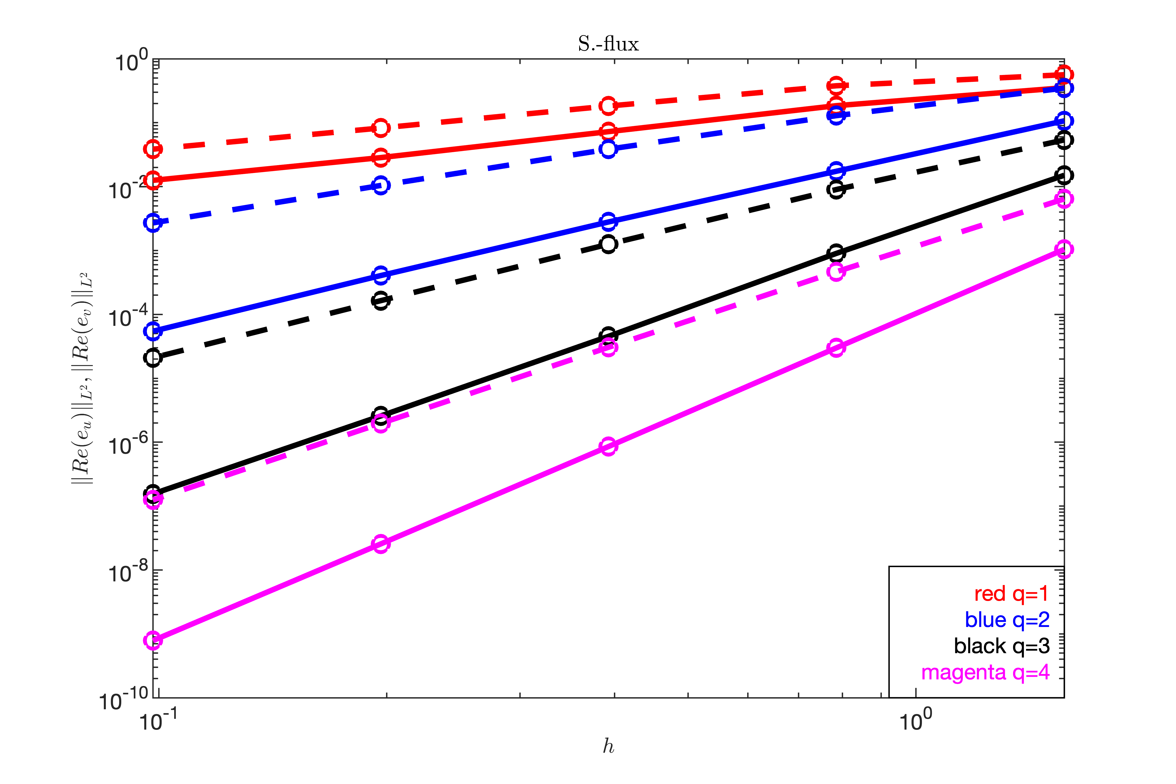
Refer to caption
Refer to caption
Refer to caption
Figure 7: L2superscript𝐿2L^{2} errors for the real parts of u𝑢u and v𝑣v for the problem  (54). The solid lines show the results of uhsubscript𝑢ℎu_{h}, while the dashed lines show the results of vhsubscript𝑣ℎv_{h}. uhsuperscript𝑢ℎu^{h} and vhsuperscript𝑣ℎv^{h} are chosen to be in the same approximation space.
\@tabular@row@before@xcolor\@tabular@row@before@xcolor\@tabular@row@before@xcolor   \@xcolor@tabular@before convergence rates of u/v𝑢𝑣u/v
\@tabular@row@before@xcolor\@tabular@row@before@xcolor\@tabular@row@before@xcolor   \@xcolor@row@after\@xcolor@row@after\@xcolor@row@afterflux/(q,s)𝑞𝑠(q,s) q=1𝑞1q=1 q=2𝑞2q=2 q=3𝑞3q=3 q=4𝑞4q=4
\@tabular@row@before@xcolor\@tabular@row@before@xcolor\@tabular@row@before@xcolor   \@xcolor@row@after\@xcolor@row@after\@xcolor@row@afterS.-flux 1.2332/0.9938 2.7304/1.7647 4.1591/2.8439   5.0882/3.9196
\@tabular@row@before@xcolor\@tabular@row@before@xcolor\@tabular@row@before@xcolor   \@xcolor@row@after\@xcolor@row@after\@xcolor@row@afterA.-flux 0.5847/-0.0306 2.1428/1.0975 3.9683/2.0289   4.8977/3.0363
\@tabular@row@before@xcolor\@tabular@row@before@xcolor\@tabular@row@before@xcolor   \@xcolor@row@after\@xcolor@row@after\@xcolor@row@afterC.-flux 2.0651/0.8774 1.9333/1.0062 4.2927/2.9930   4.8280/2.9716
\@tabular@row@before@xcolor\@tabular@row@before@xcolor\@tabular@row@before@xcolor   \@xcolor@row@after\@xcolor@row@after\@xcolor@row@after
Table 3: Linear least squares estimates of the rates of convergence from the curves in Figure 7 for the real parts of u𝑢u and v𝑣v of the problem  (54).

5 Concluding remarks

We proposed and analyzed a novel energy-based discontinuous Galerkin scheme for solving nonlinear Schrödinger equations with the wave operator. The scheme incorporates a first-order time derivative as an auxiliary variable, which reduces the second-order equation in time to a first-order system in time. By doing so, we only need to introduce one auxiliary regardless of the dimension of the problem, which improves computational efficiency by reducing the memory requirements for the variables to be solved. Moreover, the scheme is unconditionally stable without the need for penalty terms. We demonstrated the stability of the scheme for general mesh-independent numerical fluxes. We also derive suboptimal estimates of convergence in the energy norm and observe, for polynomial degrees above 111, optimal convergence in the L2superscript𝐿2L^{2} norm for the energy-conserving alternating flux as well as for dissipative methods based on the Sommerfeld flux.

Designing more general numerical fluxes than we proposed here and deriving error estimates for the corresponding schemes is an interesting direction for future study. It is also of great interest to see if the schemes we developed here can be generalized to handle stochastic versions of model (1). Utilizing the scheme developed here to study inverse problems of reconstructing model parameters from measured solution data of equation (1) is an ongoing project.

Acknowledgments

This work is partially supported by the National Science Foundation through grants DMS-1913309, DMS-1937254, and DMS-2309802.

References

  • [1] D. Appelö and T. Hagstrom, A new discontinuous Galerkin formulation for wave equations in second-order form, SIAM J. Numer. Anal., 53 (2015), pp. 2705–2726.
  • [2]  , An energy-based discontinuous Galerkin discretization of the elastic wave equation in second order form, Comput. Methods Appl. Mech. Engrg., 338 (2018), pp. 362–391.
  • [3] D. Appelö, T. Hagstrom, Q. Wang, and L. Zhang, An energy-based discontinuous Galerkin method for semilinear wave equations, J. Comput. Phys., 418 (2020), p. 109608.
  • [4] D. Appelö, L. Zhang, T. Hagstrom, and F. Li, An energy-based discontinuous Galerkin method with tame CFL numbers for the wave equation, BIT Numerical Mathematics, 63 (2023), p. 5.
  • [5] W. Bao and Y. Cai, Uniform and optimal error estimates of an exponential wave integrator sine pseudospectral method for the nonlinear Schrödinger equation with wave operator, SIAM J. Numer. Anal., 52 (2014), pp. 1103–1127.
  • [6] W. Bao, Y. Cai, and X. Zhao, A uniformly accurate multiscale time integrator pseudospectral method for the Klein–Gordon equation in the nonrelativistic limit regime, SIAM J. Numer. Anal., 52 (2014), pp. 2488–2511.
  • [7] W. Bao, X. Dong, and J. Xin, Comparisons between sine-Gordon and perturbed nonlinear Schrödinger equations for modeling light bullets beyond critical collapse, Phys. D, 239 (2010), pp. 1120–1134.
  • [8] W. Bao and X. Zhao, Comparison of numerical methods for the nonlinear Klein–Gordon equation in the nonrelativistic limit regime, J. Comput. Phys., 398 (2019), p. 108886.
  • [9] L. Bergé and T. Colin, A singular perturbation problem for an envelope equation in plasma physics, Phys. D, 84 (1995), pp. 437–459.
  • [10] P. G. Ciarlet, The finite element method for elliptic problems, SIAM, 2002.
  • [11] B. Cockburn, G. E. Karniadakis, and C.-W. Shu, Discontinuous Galerkin Methods: Theory, Computation, and Applications, vol. 11, Springer Science & Business Media, 2012.
  • [12] T. Colin and P. Fabrie, Semidiscretization in time for nonlinear Schrödinger-waves equations, Discrete Contin. Dyn. Syst., 4 (1998), pp. 671–690.
  • [13] D. Deng and Z. Li, High-order structure-preserving Du Fort–Frankel schemes and their analyses for the nonlinear Schrödinger equation with wave operator, J. Comput. Appl. Math., 417 (2023), p. 114616.
  • [14] Y. Du, L. Zhang, and Z. Zhang, Convergence analysis of a discontinuous Galerkin method for wave equations in second-order form, SIAM J. Numer. Anal., 57 (2019), pp. 238–265.
  • [15] Y. Feng, Y. Guo, and Y. Yuan, Uniform error bound of an exponential wave integrator for the long-time dynamics of the nonlinear Schrödinger equation with wave operator, arXiv:2304.00772, (2023).
  • [16] X. Gu, W. Cai, C. Jiang, and Y. Wang, Linearly implicit energy-preserving integrating factor methods for the 2D nonlinear Schrödinger equation with wave operator and convergence analysis, arXiv:2209.07710, (2022).
  • [17] B.-L. Guo and H.-X. Liang, On the problem of numerical calculation for a class of the system of nonlinear Schrödinger equations with wave operator, J. Numer. Methods Comput. Appl., 4 (1983), pp. 176–182.
  • [18] L. Guo and Y. Xu, Energy conserving local discontinuous Galerkin methods for the nonlinear Schrödinger equation with wave operator, J. Sci. Comput., 65 (2015), pp. 622–647.
  • [19] T. Hagstrom, D. Appelö, and L. Zhang, Discontinuous Galerkin methods for electromagnetic waves in dispersive media, in 2021 International Applied Computational Electromagnetics Society Symposium (ACES), IEEE, 2021, pp. 1–4.
  • [20] S. Labidi and K. Omrani, A new conservative fourth-order accurate difference scheme for the nonlinear Schrödinger equation with wave operator, Appl. Numer. Math., 173 (2022), pp. 1–12.
  • [21] H. Li, Local absorbing boundary conditions for two-dimensional nonlinear Schrödinger equation with wave operator on unbounded domain, Math. Methods Appl. Sci., 44 (2021), pp. 14382–14392.
  • [22] H. Li, X. Wu, and J. Zhang, Numerical solution of the nonlinear Schrödinger equation with wave operator on unbounded domains, Phys. Rev. E, 90 (2014), p. 033309.
  • [23] X. Li, Y. Gong, and L. Zhang, Linear high-order energy-preserving schemes for the nonlinear Schrödinger equation with wave operator using the scalar auxiliary variable approach, J. Sci. Comput., 88 (2021), p. 20.
  • [24] X. Li, L. Zhang, and S. Wang, A compact finite difference scheme for the nonlinear Schrödinger equation with wave operator, Appl. Math. Comput., 219 (2012), pp. 3187–3197.
  • [25] S. Machihara, K. Nakanishi, and T. Ozawa, Nonrelativistic limit in the energy space for nonlinear Klein–Gordon equations, Math. Ann., 322 (2002), pp. 603–621.
  • [26] K. Matsuuchi, Nonlinear interactions of counter-travelling waves, J. Phys. Soc. Japan, 48 (1980), pp. 1746–1754.
  • [27] K. Pan, J. Xia, D. He, and Q. Zhang, A three-level linearized difference scheme for nonlinear Schrödinger equation with absorbing boundary conditions, Appl. Numer. Math., 156 (2020), pp. 32–49.
  • [28] B. M. Riviere, Discontinuous Galerkin Methods For Solving Elliptic And parabolic Equations: Theory and Implementation, SIAM, 2008.
  • [29] A. Y. Schoene, On the nonrelativistic limits of the Klein–Gordon and Dirac equations, J. Math. Anal. Appl., 71 (1979), pp. 36–47.
  • [30] D. Shi and H. Zhang, Unconditional optimal error estimates and superconvergence analysis of energy-preserving FEM for general nonlinear Schrödinger equation with wave operator, Comput. Math. Appl., 128 (2022), pp. 79–95.
  • [31] J. Wang, Multisymplectic Fourier pseudospectral method for the nonlinear Schrödinger equations with wave operator, J. Comput. Math., (2007), pp. 31–48.
  • [32] T. Wang, Uniform point-wise error estimates of semi-implicit compact finite difference methods for the nonlinear Schrödinger equation perturbed by wave operator, J. Math. Anal. Appl., 422 (2015), pp. 286–308.
  • [33] T. Wang and L. Zhang, Analysis of some new conservative schemes for nonlinear Schrödinger equation with wave operator, Appl. Math. Comput., 182 (2006), pp. 1780–1794.
  • [34] J. X. Xin, Modeling light bullets with the two-dimensional sine–Gordon equation, Phys. D, 135 (2000), pp. 345–368.
  • [35] Y. Yang, H. Li, and X. Guo, A linearized energy-conservative scheme for two-dimensional nonlinear Schrödinger equation with wave operator, Appl. Math. Comput., 404 (2021), p. 126234.
  • [36] L. Zhang, A local energy-based discontinuous Galerkin method for fourth order semilinear wave equations, arXiv:2109.07033, (2021).
  • [37] L. Zhang, D. Appelö, and T. Hagstrom, Energy-based discontinuous Galerkin difference methods for second-order wave equations, Commun. Appl. Math. Comput., (2021), pp. 1–25.
  • [38] L. Zhang and Q. Chang, A conservative numerical scheme for a class of nonlinear Schrödinger equation with wave operator, Appl. Math. Comput., 145 (2003), pp. 603–612.
  • [39] L. Zhang, T. Hagstrom, and D. Appelö, An energy-based discontinuous Galerkin method for variational wave equations, Preprint.
  • [40] L. Zhang, T. Hagstrom, and D. Appelö, An energy-based discontinuous Galerkin method for the wave equation with advection, SIAM J. Numer. Anal., 57 (2019), pp. 2469–2492.