跳到论文正文
W Papers独立论文阅读器 arXiv:2311.01509 论文正文 计算阅读时间 · 0%
引用这篇论文根据当前论文元数据生成,正式投稿前建议核对。


Photon-resolved Floquet theory in open quantum systems

Georg Engelhardt engelhardt@sustech.edu.cn Shenzhen Institute for Quantum Science and Engineering, Southern University of Science and Technology, Shenzhen 518055, China International Quantum Academy, Shenzhen 518048, China Guangdong Provincial Key Laboratory of Quantum Science and Engineering, Southern University of Science and Technology, Shenzhen, 518055, China    JunYan Luo Department of Physics, Zhejiang University of Science and Technology, Hangzhou 310023, China    Victor M. Bastidas Physics and Informatics Laboratory, NTT Research, Inc., 940 Stewart Dr., Sunnyvale, California, 94085, USA Department of Chemistry, Massachusetts Institute of Technology, Cambridge, Massachusetts 02139, USA    Gloria Platero Instituto de Ciencia de Materiales de Madrid ICMM-CSIC, 28049 Madrid, Spain
Abstract

Photon-resolved Floquet theory keeps track of the photon exchange of a quantum system with a coherent driving field. It thus complements the standard full-counting statistics that counts the number of photons exchanged with incoherent photon modes giving rise to dissipation. In this paper, we introduce a unifying framework describing both situations. We develop methods suitable for an analytical evaluation of low-order cumulants of photonic probability distributions. Within this framework we analyze the two-mode Jaynes-Cummings model to demonstrate that the Photon-resolved Floquet theory and the standard full-counting statistics make consistent statistical predictions. Interestingly, we find that the photon-flux fluctuations diverge for vanishing dissipation, which can be related to an entanglement effect between the driven matter system and the driving field. To substantiate our results, we use our framework to describe efficient photon up-conversion in an ac-driven lambda system, that is characterized by a high signal-to-noise ratio. As the framework is non-perturbative and predicts fluctuations, it paves the way towards non-perturbative spectroscopy, which will assist to improve metrological methods.

pacs:

I Introduction

Full-counting statistics (FCS) is a successful theoretical framework finding broad applications in many fields of quantum physics [1, 2, 3, 4, 5, 6]. FCS was originally developed by Mandel in quantum optics to describe spontaneous photon emission [7], and has been later adapted to electron transport through mesoscopic systems by Levitov and Lesovik [8]. The formalism also describes thermal transport in heat engines and other thermal devices [9]. More recently, a Floquet version of the FCS has been developed to describe electron transport through periodically-driven quantum dots [10, 11, 12, 13]. Moreover, within the framework of FCS, feedback control protocols have been developed which can suppress transport noise [14].

Refer to caption
Figure 1: (a) and (b) Sketch of a quantum system in state |ϕ⟩ketitalic-ϕ\left|\phi\right> which is driven by two coherent light fields and coupled to a continuum of reservoir of optical and microwave photon modes, respectively, with coupling strength γ𝛾\gamma. In the case of optical photons, the atom is coupled to two optical cavities and a continuum environment of photonic modes, while in the case of microwave photons, a nonlinear LC resonator (transmon) is coupled to two LC resonators acting as cavities. Due to the light-matter interaction, photons become redistributed between the driving modes and the reservoir. c) The resulting photonic probability distributions can be measured and predicted within the framework introduced in Sec. II. d) Photonic probability distribution of the coherent photon mode k=1𝑘1k=1 in closed (γ=0𝛾0\gamma=0) and open (γ>0𝛾0\gamma>0) quantum systems for three different light-matter interaction durations t0subscript𝑡0t_{0}, t1subscript𝑡1t_{1}, t2subscript𝑡2t_{2}. For γ=0𝛾0\gamma=0, the photonic dynamics is determined by the Floquet states: (l.h.s.) photonic probability distribution for an initial Floquet state; (r.h.s.) photonic probability distribution for an initial superposition of two Floquet states. For long times, the initial superposition state leads to a light-matter entangled state in the Floquet-state basis. For γ>0𝛾0\gamma>0, the dissipation induces jumps between the Floquet states. As a consequence, the light-matter entanglement depicted in the r.h.s. is gradually destroyed. The dynamics has been calculated for the Jaynes-Cummings model in Sec. III, for ϵ=0italic-ϵ0\epsilon=0, Ω1=Ω2=gsubscriptΩ1subscriptΩ2𝑔\Omega_{1}=\Omega_{2}=g, φ1=0subscript𝜑10\varphi_{1}=0, φ2=π/2subscript𝜑2𝜋2\varphi_{2}=\pi/2, and γ=0.01​g𝛾0.01𝑔\gamma=0.01g.

However, the standard FCS fails to correctly predict photon exchange with coherent photonic driving fields which is important in stimulated absorption and emission processes. The FCS formalism is fundamentally based on two-point projective measurements that project the state of photons at the beginning and the end of the time evolution to extract the photon statistics. Formally, the initial projection destroys coherences at the initial time [15]. Thus, the resulting state after the projection is not a coherent state. To circumvent this problem, the Photon-resolved Floquet theory (PRFT) has been recently developed  [16]. This framework replaces the problematic two-point projective measurement by a suitable two-point tomographic measurement [17]. Thereby, two batches of experimental runs are independently carried out, the first batch measures the photon statistics only at the initial time, while the second batch measures the statistics only at the final time. The PRFT predicts then the differences between the initial and final measurement statistics.

By modifying concepts and methods of the standard FCS, the PRFT is capable to predict the photonic probability distribution by integration of the semiclassical equations of motion, allowing for a simple analytical and numerical treatment. Intriguingly, the PRFT makes correct predictions in a deep-quantum regime beyond the capability of common semiclassical methods. It predicts light-matter entanglement in the Floquet-state basis, which has been suggested as a resource for highly-efficient quantum communication protocols using coherent states instead of single photons [16]. These predictions are beyond typical semiclassical light-matter frameworks such as methods from standard non-linear spectroscopy [18] or perturbation theory in the Floquet basis [19, 20, 21, 22].

Unification of the standard FCS and the PRFT is needed to describe systems where both spontaneous and stimulated emission are present, which is the aim of the present work. Sketches of typical setups consisting of a quantum systems, two driving modes, and a dissipative photonic environment (i.e., a bath) in a cavity and circuit quantum electrodynamics experiments are depicted in Fig. 1(a) and Fig. 1(b), respectively. The first challenge is to modify the PRFT, that has been originally developed for closed quantum systems, to open quantum systems, in which the FCS is valid. The second challenge is to ensure that all photons are consistently counted under the constraint of photon conservation: Energy lost in the coherent photon modes must eventually re-appear in the incoherent photon ones. It is interesting to note that, while the FCS has been originally developed in quantum optics, the theoretical framework has revealed its full potential in mesoscopic electron transport, where charges can tunnel in a multi-terminal setup. The PRFT takes advantage of the rich methodology of mesoscopic transport, and establishes a quantum-optical framework that describes photon flux between various photonic modes, which can be likewise viewed as a multi-terminal setup.

In this paper, we address the counting statistics of quantum systems which are both coherently driven and coupled to a continuum of incoherent photon modes, and develop a unifying framework which is valid for open quantum systems. Moreover, we develop three analytical methods to characterize the photonic probability distributions: (i) expansion of the characteristic polynomial of the Liouvillian in a power series of the counting field; (ii) generalizing the stationary perturbation theory known for Hermitian system to non-Hermitian ones; and (iii) modifying well-established adiabatic elimination procedures.

Taking a two-mode generalization of the Jaynes-Cummings model as an example, we demonstrate that our unified formalism consistently describes the photon statistics of coherent and incoherent photon modes. Moreover, we investigate the fate of the intriguing light-matter entanglement in situations where the system is subject to dissipation. The findings are illustrated in Fig. 1(c). In an isolated quantum system, light and matter becomes entangled in the Floquet basis. When dissipation is present, the entanglement decreases during the time evolution. Intriguingly, this effect leads to diverging photon flux fluctuations for a small dissipation. As a more sophisticated application, we apply the formalism to an ac-driven lambda system, and show how to deploy it as a frequency-conversion device of coherent light characterized by a high signal-to-noise ratio.

Importantly, the theory proposed in the present work paves the way to a non-perturbative spectroscopic framework that allows for statistical predictions beyond standard methods from non-linear spectroscopy [18] and quantum optics [23], which is of utmost importance in chemistry [24] and biology [25]. For instance, we derive exact expressions for the photon flux and its fluctuations in the paradigmatic two-mode Jaynes-Cummings model, that are non-perturbative in all parameters. These findings will constitute a basis for improved metrological methods with impact on other areas of physics such as dark-matter detection [26]. In fact, increasing effort is committed to develop highly-sensitive dark-matter detectors based on co-magnetometers, that use lasers to measure the magnetic state of atoms via the Faraday effect [27, 28]. Floquet systems are deployed to improve the sensitivity of the so-called Floquet co-magnetometers [29]. Similar approaches are used to improve the standard of atomic clocks [30, 31]. The theoretical framework developed here will pave the way to develop stochastic models that predict measurement statistics, and can thus help to further enhance the sensitivity in such experiments.

Besides optics, the framework developed here can also find application in fast read-out protocols required in quantum computation devices based on superconducting flux qubits [32] and silicon quantum dots [33]. In particular, recent developments in the field of arrays of superconducting qubits [34, 32], exploit the coupling of the qubit to resonators to perform dispersive readout of the qubit state [35]. In addition, the qubit is coupled to external control lines and tunable couplers that enable to apply microwave pulses to drive the dynamics of the system [36, 37]. As the qubit is coupled to control lines and resonators for read out, it is also under the effect of the external environment [38] and understanding the statistics of the photons is of extreme interest in the field [39, 40, 41]. Dispersive read-out schemes typically employ off-resonance configurations, which limits the read-out speed. The exact photon statistics predicted by the present model would in principle allow for on-resonance read-out protocols, which could significantly reduce the read-out time.

This paper is organized as follows. In Sec. II, we introduce a general framework that unifies standard FCS and PRFT. In Sec. III, we apply the framework to a multimode Jaynes-Cummings model and investigate the fate of the light-matter entanglement in open quantum systems. In Sec. IV, we investigate an ac-driven lambda system for its application as an efficient frequency conversion device. In Sec. V, we conclude and discuss our results. We provide detailed derivations and an introduction to various analytical methods in the Appendices.

II Unifying framework of FCS and PRFT

Here, we establish a unifying framework allowing for simultaneously counting coherent and incoherent photon processes. Moreover, we explain how to evaluate cumulants in the long-time limit using Floquet theory in terms of the eigenvalues of the stroboscopic Liouvillian operator.

II.1 System

Figure 1(a) depicts a quantum system driven by two coherent light fields (e.g., in optical cavities), that is coupled to a continuum of modes, to which it incoherently emits photons. To describe both effects on an equal footing, we start from a fully-quantized light-matter Hamiltonian

H^=H^0+∑k=1ND+NBωk​a^k†​a^k+∑k=1ND+NBg~​V^k​(a^k†+a^k),^𝐻subscript^𝐻0superscriptsubscript𝑘1subscript𝑁Dsubscript𝑁Bsubscript𝜔𝑘superscriptsubscript^𝑎𝑘†subscript^𝑎𝑘superscriptsubscript𝑘1subscript𝑁Dsubscript𝑁B~𝑔subscript^𝑉𝑘superscriptsubscript^𝑎𝑘†subscript^𝑎𝑘\hat{H}=\hat{H}_{0}+\sum_{k=1}^{N_{\text{D}}+N_{\text{B}}}\omega_{k}\hat{a}_{k}^{\dagger}\hat{a}_{k}+\sum_{k=1}^{N_{\text{D}}+N_{\text{B}}}\tilde{g}\hat{V}_{k}\left(\hat{a}_{k}^{\dagger}+\hat{a}_{k}\right), (1)

where H^0subscript^𝐻0\hat{H}_{0} denotes the matter Hamiltonian, and the photonic creation a^k†superscriptsubscript^𝑎𝑘†\hat{a}_{k}^{\dagger} and annihilation a^ksubscript^𝑎𝑘\hat{a}_{k} operators quantize the electromagnetic field. The light-matter interaction is described by V^ksubscript^𝑉𝑘\hat{V}_{k} acting on the matter system, where g~~𝑔\tilde{g} parameterizes the interaction strength. At this point it is important to emphasize the generality of our approach. The Hamiltonian in Eq. (1) is a general description of a system coupled to a bosonic enviromnent. Besides in quantum optics, one encounters this configuration in circuit quantum electrodynamics, where LC resonators analogous to cavities can be coupled to transmons acting as qubits [42], which is sketched in Fig. 1(b). In fact, the Hamiltonian we discuss in this work is also relevant for the coupling of a superconducting qubit to a collection of acoustic modes that can be exploited as hardware-efficient implementation of a quantum random access memory (QRAM) [43].

The photonic modes are distributed into two categories: The first NDsubscript𝑁DN_{\text{D}} photonic modes coherently drive the matter system. Their joint initial state shall be given by a product of coherent states

|A0⟩=∏k=1ND|αk​ei​φk⟩,ketsubscript𝐴0superscriptsubscriptproduct𝑘1subscript𝑁Dketsubscript𝛼𝑘superscript𝑒𝑖subscript𝜑𝑘\left|A_{0}\right>=\prod_{k=1}^{N_{\text{D}}}\left|\alpha_{k}e^{i\varphi_{k}}\right>, (2)

that are defined as the eigenstates of annihilation operators a^k​|αk​ei​φk⟩=αk​ei​φk​|αk​ei​φk⟩subscript^𝑎𝑘ketsubscript𝛼𝑘superscript𝑒𝑖subscript𝜑𝑘subscript𝛼𝑘superscript𝑒𝑖subscript𝜑𝑘ketsubscript𝛼𝑘superscript𝑒𝑖subscript𝜑𝑘\hat{a}_{k}\left|\alpha_{k}e^{i\varphi_{k}}\right>=\alpha_{k}e^{i\varphi_{k}}\left|\alpha_{k}e^{i\varphi_{k}}\right> with real-valued amplitudes αksubscript𝛼𝑘\alpha_{k} and phases φksubscript𝜑𝑘\varphi_{k}. In the semiclassical limit αk≫1much-greater-thansubscript𝛼𝑘1\alpha_{k}\gg 1, it is justified to replace the photonic operators by their expectation values in the Heisenberg picture a^k​(t)→αk​e−i​ωk​t+i​φk→subscript^𝑎𝑘𝑡subscript𝛼𝑘superscript𝑒𝑖subscript𝜔𝑘𝑡𝑖subscript𝜑𝑘\hat{a}_{k}(t)\rightarrow\alpha_{k}e^{-i\omega_{k}t+i\varphi_{k}}. This establishes a semiclassical Hamiltonian that describes the dynamics of the matter system [16]. This is the case which we consider in the present work. Conceptually, we focus here on coherent light in a cavity setup, while application of the PRFT to propagating light fields (e.g., laser light) will be considered in relation to spectroscopy in a future work. However, we note here that these two situations are almost identical on a formal level.

The photonic modes k=ND+1,…,ND+NB𝑘subscript𝑁D1…subscript𝑁Dsubscript𝑁Bk=N_{\text{D}}+1,\dots,N_{\text{D}}+N_{\text{B}} form a continuum (i.e., a bath with NB≫1much-greater-thansubscript𝑁B1N_{\text{B}}\gg 1) and are assumed to be initially in a thermal state

ρB=1Z​exp⁡(−β​∑k=ND+1ND+NBωk​a^k†​a^k),subscript𝜌B1𝑍𝛽superscriptsubscript𝑘subscript𝑁D1subscript𝑁Dsubscript𝑁Bsubscript𝜔𝑘superscriptsubscript^𝑎𝑘†subscript^𝑎𝑘\rho_{\text{B}}=\frac{1}{Z}\exp\left(-\beta\sum_{k=N_{\text{D}}+1}^{N_{\text{D}}+N_{\text{B}}}\omega_{k}\hat{a}_{k}^{\dagger}\hat{a}_{k}\right), (3)

where Z𝑍Z is the partition function. In contrast to a coherent state, the thermal state is diagonal in the photon-number basis. Thus, these modes act incoherently on the matter system and give rise to dissipation. Throughout the paper, the initial state of the light-matter system is assumed to be

ρ​(0)=ρS​(0)⊗ρB⊗|A0⟩​⟨A0|,𝜌0tensor-productsubscript𝜌S0subscript𝜌𝐵ketsubscript𝐴0brasubscript𝐴0\rho(0)=\rho_{\text{S}}(0)\otimes\rho_{B}\otimes\left|A_{0}\right>\left<A_{0}\right|, (4)

where ρS​(0)subscript𝜌S0\rho_{\text{S}}(0) is the initial state of the matter system.

II.2 Coherent and incoherent counting of photons

The different initial conditions of the photonic fields given in Eq. (2) and (3) require a different physical definition of the counting statistics. The emission and absorption of incoherent reservoir photons can be treated accurately using standard FCS, that assumes two-point projective measurements carried out at times t=0𝑡0t=0 and t>0𝑡0t>0 in each experimental run [16, 15, 8]. At both times, the system is projected onto the photon number basis, and the number difference is tracked by the moment and cumulant generating functions. In contrast, the PRFT counts the photons of the driving field in terms of two-point tomographic measurements, at which the statistics of the photon field are obtained at times t=0𝑡0t=0 and t>0𝑡0t>0 in independent experimental runs [16]. In doing so, the coherences, that are responsible for the oscillating behavior of the driving field, are preserved. The concepts of the standard FCS and the PRFT are summarized in Appendix. A.

Despite their fundamental differences, both formalisms can be simultaneously applied. We are interested into the statistics of the photonic occupations n^k=a^k†​a^ksubscript^𝑛𝑘superscriptsubscript^𝑎𝑘†subscript^𝑎𝑘\hat{n}_{k}=\hat{a}_{k}^{\dagger}\hat{a}_{k}. As explained in Appendix A, the information about the photonic probability distributions is contained in the moment-generating function,

M𝝃,𝝌​(t)subscript𝑀𝝃𝝌𝑡\displaystyle M_{\boldsymbol{\xi},\boldsymbol{\chi}}(t) =12​tr​[U^𝝃/2,𝝌​(t)​e−i​𝝌⋅𝒏^D​ρ​(0)​U^−𝝃/2,0†​(t)]absent12trdelimited-[]subscript^𝑈𝝃2𝝌𝑡superscript𝑒⋅𝑖𝝌subscript^𝒏D𝜌0subscriptsuperscript^𝑈†𝝃20𝑡\displaystyle=\frac{1}{2}\text{tr}\left[\hat{U}_{\boldsymbol{\xi}/2,\boldsymbol{\chi}}(t)e^{-i\boldsymbol{\chi}\cdot\hat{\boldsymbol{n}}_{\text{D}}}\rho(0)\hat{U}^{\dagger}_{-\boldsymbol{\xi}/2,0}(t)\right]
+12​tr​[U^𝝃/2,0​(t)​ρ​(0)​e−i​𝝌⋅𝒏^D​U^−𝝃/2,−𝝌†​(t)],12trdelimited-[]subscript^𝑈𝝃20𝑡𝜌0superscript𝑒⋅𝑖𝝌subscript^𝒏Dsubscriptsuperscript^𝑈†𝝃2𝝌𝑡\displaystyle+\frac{1}{2}\text{tr}\left[\hat{U}_{\boldsymbol{\xi}/2,0}(t)\rho(0)e^{-i\boldsymbol{\chi}\cdot\hat{\boldsymbol{n}}_{\text{D}}}\hat{U}^{\dagger}_{-\boldsymbol{\xi}/2,-\boldsymbol{\chi}}(t)\right],

where the generalized time-evolution operator is given as

U^𝝃,𝝌​(t)subscript^𝑈𝝃𝝌𝑡\displaystyle\hat{U}_{\boldsymbol{\xi},\boldsymbol{\chi}}(t) =\displaystyle= exp⁡(−i​H^𝝃,𝝌​t),𝑖subscript^𝐻𝝃𝝌𝑡\displaystyle\exp\left(-i\hat{H}_{\boldsymbol{\xi},\boldsymbol{\chi}}t\right),
H^𝝃,𝝌subscript^𝐻𝝃𝝌\displaystyle\hat{H}_{\boldsymbol{\xi},\boldsymbol{\chi}} =\displaystyle= e−i​(𝝌⋅𝒏^D+𝝃⋅𝒏^B)​H^​ei​(𝝌⋅𝒏^D+𝝃⋅𝒏^B).superscript𝑒𝑖⋅𝝌subscript^𝒏D⋅𝝃subscript^𝒏B^𝐻superscript𝑒𝑖⋅𝝌subscript^𝒏D⋅𝝃subscript^𝒏B\displaystyle e^{-i(\boldsymbol{\chi}\cdot\hat{\boldsymbol{n}}_{\text{D}}+\boldsymbol{\xi}\cdot\hat{\boldsymbol{n}}_{\text{B}})}\hat{H}e^{i(\boldsymbol{\chi}\cdot\hat{\boldsymbol{n}}_{\text{D}}+\boldsymbol{\xi}\cdot\hat{\boldsymbol{n}}_{\text{B}})}. (6)

We have introduced the notation 𝝌⋅𝒏^D=∑k=1NDχk​n^k⋅𝝌subscript^𝒏Dsuperscriptsubscript𝑘1subscript𝑁Dsubscript𝜒𝑘subscript^𝑛𝑘\boldsymbol{\chi}\cdot\hat{\boldsymbol{n}}_{\text{D}}=\sum_{k=1}^{N_{\text{D}}}\chi_{k}\hat{n}_{k} and 𝝃⋅𝒏^B=∑k=ND+1ND+NBξk​n^k⋅𝝃subscript^𝒏Bsuperscriptsubscript𝑘subscript𝑁D1subscript𝑁Dsubscript𝑁Bsubscript𝜉𝑘subscript^𝑛𝑘\boldsymbol{\xi}\cdot\hat{\boldsymbol{n}}_{\text{B}}=\sum_{k=N_{\text{D}}+1}^{N_{\text{D}}+N_{\text{B}}}\xi_{k}\hat{n}_{k}, where the counting fields χksubscript𝜒𝑘\chi_{k} and ξksubscript𝜉𝑘\xi_{k} are tracking the photons exchanged with the coherent driving fields and the incoherent bath modes, respectively. For convenience, the counting fields have been arranged in vectors 𝝌=(χ1,…,χND)𝝌subscript𝜒1…subscript𝜒subscript𝑁D\boldsymbol{\chi}=\left(\chi_{1},\dots,\chi_{N_{\text{D}}}\right) and 𝝃=(ξND+1,…,ξND+NB)𝝃subscript𝜉subscript𝑁D1…subscript𝜉subscript𝑁Dsubscript𝑁B\boldsymbol{\xi}=\left(\xi_{N_{\text{D}}+1},\dots,\xi_{N_{\text{D}}+N_{\text{B}}}\right). As we see from Eq. (LABEL:eq:def:momentGeneratingFkt_exact), the counting fields 𝝌𝝌\boldsymbol{\chi} and 𝝃𝝃\boldsymbol{\xi} enter the moment-generating function in a different way. This reflects the underlying definition of the counting statistics in terms of the two-point tomographic and projective measurements, respectively. The operation tr​[∙]trdelimited-[]∙\text{tr}\left[\bullet\right] in Eq. (LABEL:eq:def:momentGeneratingFkt_exact) denotes the trace over all degrees of freedom, i.e., of the system, driving modes, and bath.

The joint photonic probability distribution can be obtained by a Fourier transformation of the moment-generating function

p𝒏,𝒎​(t)=∫02​πd​𝝌ND(2​π)ND​∫02​πd​𝝃NB(2​π)NB​M𝝃,𝝌​(t)​ei​(𝒏⋅𝝌+𝒎⋅𝝃),subscript𝑝𝒏𝒎𝑡superscriptsubscript02𝜋𝑑superscript𝝌subscript𝑁Dsuperscript2𝜋subscript𝑁Dsuperscriptsubscript02𝜋𝑑superscript𝝃subscript𝑁Bsuperscript2𝜋subscript𝑁Bsubscript𝑀𝝃𝝌𝑡superscript𝑒𝑖⋅𝒏𝝌⋅𝒎𝝃p_{\boldsymbol{n},\boldsymbol{m}}(t)=\int_{0}^{2\pi}\frac{d\boldsymbol{\chi}^{N_{\text{D}}}}{(2\pi)^{N_{\text{D}}}}\int_{0}^{2\pi}\frac{d\boldsymbol{\xi}^{N_{\text{B}}}}{(2\pi)^{N_{\text{B}}}}M_{\boldsymbol{\xi},\boldsymbol{\chi}}(t)e^{i(\boldsymbol{n}\cdot\boldsymbol{\chi}+\boldsymbol{m}\cdot\boldsymbol{\xi})}, (7)

where the photon numbers 𝒏=(n1,…,nND)𝒏subscript𝑛1…subscript𝑛subscript𝑁𝐷\boldsymbol{n}=(n_{1},\dots,n_{N_{D}}) refer to the total number of photons in the coherent modes, while the photon numbers 𝒎=(mND+1,…,mND+NB)𝒎subscript𝑚subscript𝑁𝐷1…subscript𝑚subscript𝑁𝐷subscript𝑁𝐵\boldsymbol{m}=(m_{N_{D}+1},\dots,m_{N_{D}+N_{B}}) refer to the number of photons having entered the incoherent photon modes since time t=0𝑡0t=0. The notation ∫02​π𝑑𝝌ND=d​χ1​…​d​χNDsuperscriptsubscript02𝜋differential-dsuperscript𝝌subscript𝑁D𝑑subscript𝜒1…𝑑subscript𝜒subscript𝑁D\int_{0}^{2\pi}d\boldsymbol{\chi}^{N_{\text{D}}}=d\chi_{1}\dots d\chi_{N_{\text{D}}} denotes a multidimensional integration (likewise for 𝝃𝝃\boldsymbol{\xi}).

Alternatively, one can describe the probability distribution in terms of its cumulants, which can be calculated via the cumulant-generating function K𝝃,𝝌​(t)≡log⁡M𝝃,𝝌​(t)subscript𝐾𝝃𝝌𝑡subscript𝑀𝝃𝝌𝑡K_{\boldsymbol{\xi},\boldsymbol{\chi}}(t)\equiv\log M_{\boldsymbol{\xi},\boldsymbol{\chi}}(t). The cumulants are defined via

κk(m)​(t)=dmd​(−i​ζk)m​K𝝃,𝝌​(t)|𝝃=0,𝝌=0,superscriptsubscript𝜅𝑘𝑚𝑡evaluated-atsuperscript𝑑𝑚𝑑superscript𝑖subscript𝜁𝑘𝑚subscript𝐾𝝃𝝌𝑡formulae-sequence𝝃0𝝌0\kappa_{k}^{(m)}(t)=\left.\frac{d^{m}}{d(-i\zeta_{k})^{m}}K_{\boldsymbol{\xi},\boldsymbol{\chi}}(t)\right|_{\boldsymbol{\xi}=0,\boldsymbol{\chi}=0}, (8)

where ζksubscript𝜁𝑘\zeta_{k} refers to χksubscript𝜒𝑘\chi_{k} for k≤ND𝑘subscript𝑁Dk\leq N_{\text{D}} and or ξksubscript𝜉𝑘\xi_{k} for k>ND𝑘subscript𝑁Dk>N_{\text{D}}, respectively. The first two cumulants

κk(1)​(t)superscriptsubscript𝜅𝑘1𝑡\displaystyle\kappa_{k}^{(1)}(t) =\displaystyle= ⟨n^k​(t)⟩=n¯k​(t),delimited-⟨⟩subscript^𝑛𝑘𝑡subscript¯𝑛𝑘𝑡\displaystyle\left<\hat{n}_{k}(t)\right>=\overline{n}_{k}(t),
κk(2)​(t)superscriptsubscript𝜅𝑘2𝑡\displaystyle\kappa_{k}^{(2)}(t) =\displaystyle= ⟨n^k2​(t)⟩−⟨n^k​(t)⟩2=σk2​(t)delimited-⟨⟩superscriptsubscript^𝑛𝑘2𝑡superscriptdelimited-⟨⟩subscript^𝑛𝑘𝑡2superscriptsubscript𝜎𝑘2𝑡\displaystyle\left<\hat{n}_{k}^{2}(t)\right>-\left<\hat{n}_{k}(t)\right>^{2}=\sigma_{k}^{2}(t) (9)

are the mean n¯ksubscript¯𝑛𝑘\overline{n}_{k} and the variance σk2superscriptsubscript𝜎𝑘2\sigma_{k}^{2} of the photonic distribution, respectively. Likewise, one can calculate correlations between different photon modes by evaluating mixed derivatives.

II.3 Semiclassical dynamics in an open quantum systems

Because of the large number of photon modes in the fully-quantized Hamiltonian and the infinite-sized Hilbert space of each mode, the dynamics of the moment-generating function in Eq. (LABEL:eq:def:momentGeneratingFkt_exact) cannot be solved exactly in general. Instead, effective approaches must be applied to determine the time evolution of the reduced density matrix

ρL,𝝃,𝝌​(t)≡trD,B​[U^𝝃/2,𝝌​(t)​e−i​𝝌⋅𝒏^D​ρ​(0)​U^−𝝃/2,𝟎†​(t)],subscript𝜌L𝝃𝝌𝑡subscripttrD,Bdelimited-[]subscript^𝑈𝝃2𝝌𝑡superscript𝑒⋅𝑖𝝌subscript^𝒏D𝜌0subscriptsuperscript^𝑈†𝝃20𝑡\rho_{\text{L},\boldsymbol{\xi},\boldsymbol{\chi}}(t)\equiv\text{tr}_{\text{D,B}}\left[\hat{U}_{\boldsymbol{\xi}/2,\boldsymbol{\chi}}(t)e^{-i\boldsymbol{\chi}\cdot\hat{\boldsymbol{n}}_{\text{D}}}\rho(0)\hat{U}^{\dagger}_{-\boldsymbol{\xi}/2,\boldsymbol{0}}(t)\right], (10)

whose trace determines the first term of the moment-generating function in Eq. (LABEL:eq:def:momentGeneratingFkt_exact). Here, trD,B​[∙]subscripttrD,Bdelimited-[]∙\text{tr}_{\text{D,B}}\left[\bullet\right] denotes the partial trace over the driving and bath photon modes. Several methods have been developed to describe the time-evolution of open quantum systems, such as the quantum master equation [44], the Redfield equation [45], the polaron-transformed master equation [46, 47], the hierarchy equations of motion [48], and other more advanced approaches [49]. Here, we apply the quantum Langevin approach [50, 51, 23], and obtain a quantum-master equation in Lindblad form

dd​t​ρL,𝝃,𝝌𝑑𝑑𝑡subscript𝜌L𝝃𝝌\displaystyle\frac{d}{dt}\rho_{\text{L},\boldsymbol{\xi},\boldsymbol{\chi}} =\displaystyle= −i​[ℋ𝝌​(t)​ρL,𝝃,𝝌−ρL,𝝃,𝝌​ℋ𝟎​(t)]𝑖delimited-[]subscriptℋ𝝌𝑡subscript𝜌L𝝃𝝌subscript𝜌L𝝃𝝌subscriptℋ0𝑡\displaystyle-i\left[\mathcal{H}_{\boldsymbol{\chi}}(t)\rho_{\text{L},\boldsymbol{\xi},\boldsymbol{\chi}}-\rho_{\text{L},\boldsymbol{\xi},\boldsymbol{\chi}}\mathcal{H}_{\boldsymbol{0}}(t)\right] (11)
+∑jγj​D𝝃​[Sj]​ρL,𝝃,𝝌,subscript𝑗subscript𝛾𝑗subscript𝐷𝝃delimited-[]subscript𝑆𝑗subscript𝜌L𝝃𝝌\displaystyle+\mathcal{\sum}_{j}\gamma_{j}D_{\boldsymbol{\xi}}\left[S_{j}\right]\rho_{\text{L},\boldsymbol{\xi},\boldsymbol{\chi}},

where the semiclassical Hamiltonian

ℋ^𝝌​(t)=H^0+∑k=1NDg~​V^k​αk​cos⁡(ωk​t+φk+χk)subscript^ℋ𝝌𝑡subscript^𝐻0superscriptsubscript𝑘1subscript𝑁D~𝑔subscript^𝑉𝑘subscript𝛼𝑘subscript𝜔𝑘𝑡subscript𝜑𝑘subscript𝜒𝑘\hat{\mathcal{H}}_{\boldsymbol{\chi}}(t)=\hat{H}_{0}+\sum_{k=1}^{N_{\text{D}}}\tilde{g}\hat{V}_{k}\alpha_{k}\cos\left(\omega_{k}t+\varphi_{k}+\chi_{k}\right) (12)

describes the action of the coherent modes in Eq. (1). The impact of the incoherent modes is encoded into the dissipator D𝝃​[S^j]​ρLsubscript𝐷𝝃delimited-[]subscript^𝑆𝑗subscript𝜌LD_{\boldsymbol{\xi}}\left[\hat{S}_{j}\right]\rho_{\text{L}} with system operators S^jsubscript^𝑆𝑗\hat{S}_{j}, which are determined by the V^ksubscript^𝑉𝑘\hat{V}_{k} and the exact form of the Hamiltonian in Eq. (1).

The second term of the moment-generating function in Eq. (LABEL:eq:def:momentGeneratingFkt_exact) can be obtained by taking the trace of

ρR,𝝃,𝝌​(t)≡trD,B​[U^𝝃/2,0​(t)​ρ​(0)​e−i​𝝌⋅𝒏^D​U^−𝝃/2,−𝝌†​(t)].subscript𝜌R𝝃𝝌𝑡subscripttrD,Bdelimited-[]subscript^𝑈𝝃20𝑡𝜌0superscript𝑒⋅𝑖𝝌subscript^𝒏Dsubscriptsuperscript^𝑈†𝝃2𝝌𝑡\rho_{\text{R},\boldsymbol{\xi},\boldsymbol{\chi}}(t)\equiv\text{tr}_{\text{D,B}}\left[\hat{U}_{\boldsymbol{\xi}/2,0}(t)\rho(0)e^{-i\boldsymbol{\chi}\cdot\hat{\boldsymbol{n}}_{\text{D}}}\hat{U}^{\dagger}_{-\boldsymbol{\xi}/2,-\boldsymbol{\chi}}(t)\right]. (13)

Assuming that the dissipators D𝝃​[∙]subscript𝐷𝝃delimited-[]∙D_{\boldsymbol{\xi}}\left[\bullet\right] are invariant under Hermitian conjugation, one can show that

ρR,𝝃,𝝌​(t)=ρL,𝝃,−𝝌†​(t),subscript𝜌R𝝃𝝌𝑡superscriptsubscript𝜌L𝝃𝝌†𝑡\rho_{\text{R},\boldsymbol{\xi},\boldsymbol{\chi}}(t)=\rho_{\text{L},\boldsymbol{\xi},-\boldsymbol{\chi}}^{\dagger}(t), (14)

such that the full information about the counting statistics is solely contained in ρL,𝝃,𝝌​(t)subscript𝜌L𝝃𝝌𝑡\rho_{\text{L},\boldsymbol{\xi},\boldsymbol{\chi}}(t), which we investigate in the following. Noteworthy, as ρL/R,𝝃,𝝌subscript𝜌L/R𝝃𝝌\rho_{\text{L/R},\boldsymbol{\xi},\boldsymbol{\chi}} is not Hermitian and tr​[ρL/R,𝝃,𝝌]≠1trdelimited-[]subscript𝜌L/R𝝃𝝌1\text{tr}\left[\rho_{\text{L/R},\boldsymbol{\xi},\boldsymbol{\chi}}\right]\neq 1 in general, these objects are strictly speaking no density matrices. Yet, these generalized density matrices can be considered as mathematical tools that trace the photons exchanged with the photonic modes. For (𝝃,𝝌)=(𝟎,𝟎)𝝃𝝌00(\boldsymbol{\xi},\boldsymbol{\chi})=(\boldsymbol{0},\boldsymbol{0}), they reduce to the common density matrix of the matter system, i.e., ρL/R,𝟎,𝟎​(t)=ρS​(t)subscript𝜌L/R00𝑡subscript𝜌S𝑡\rho_{\text{L/R},\boldsymbol{0},\boldsymbol{0}}(t)=\rho_{\text{S}}(t).

Using the semiclassical dynamics of the reduced density matrix, the moment-generating function in Eq. (LABEL:eq:def:momentGeneratingFkt_exact) can be expressed as

M𝝃,𝝌​(t)=Mdy,𝝃,𝝌​(t)​M𝝃,𝝌​(0),subscript𝑀𝝃𝝌𝑡subscript𝑀dy𝝃𝝌𝑡subscript𝑀𝝃𝝌0\displaystyle M_{\boldsymbol{\xi},\boldsymbol{\chi}}(t)=M_{\text{dy},\boldsymbol{\xi},\boldsymbol{\chi}}(t)M_{\boldsymbol{\xi},\boldsymbol{\chi}}(0), (15)

where the dynamical moment-generating function is given by

Mdy,𝝃,𝝌​(t)=tr​[ρL,𝝃,𝝌​(t)+ρR,𝝃,𝝌​(t)],subscript𝑀dy𝝃𝝌𝑡trdelimited-[]subscript𝜌L𝝃𝝌𝑡subscript𝜌R𝝃𝝌𝑡\displaystyle M_{\text{dy},\boldsymbol{\xi},\boldsymbol{\chi}}(t)=\text{tr}\left[\rho_{\text{L},\boldsymbol{\xi},\boldsymbol{\chi}}(t)+\rho_{\text{R},\boldsymbol{\xi},\boldsymbol{\chi}}(t)\right], (16)

and ρL,𝝃,𝝌​(t)subscript𝜌L𝝃𝝌𝑡\rho_{\text{L},\boldsymbol{\xi},\boldsymbol{\chi}}(t) is the solution of Eq. (11) with initial condition ρL,𝝃,𝝌​(0)=ρS​(0)subscript𝜌L𝝃𝝌0subscript𝜌S0\rho_{\text{L},\boldsymbol{\xi},\boldsymbol{\chi}}(0)=\rho_{\text{S}}(0). Details about the derivations can be found in Appendix A. The moment-generating function at initial time t=0𝑡0t=0 is given by

M𝝃,𝝌​(0)=⟨A0|e−i​𝝌⋅𝒏^D|A0⟩.subscript𝑀𝝃𝝌0quantum-operator-productsubscript𝐴0superscript𝑒⋅𝑖𝝌subscript^𝒏Dsubscript𝐴0M_{\boldsymbol{\xi},\boldsymbol{\chi}}(0)=\left<A_{0}\right|e^{-i\boldsymbol{\chi}\cdot\hat{\boldsymbol{n}}_{\text{D}}}\left|A_{0}\right>. (17)

The initial moment-generating function contains the information about the photon statistics of the coherent modes, which are determined in the initial tomographic measurement. In contrast, M𝝃,𝝌​(0)subscript𝑀𝝃𝝌0M_{\boldsymbol{\xi},\boldsymbol{\chi}}(0) does not depend on the state of the incoherent modes. This reflects the projective counting protocol of the incoherent photons, that starts counting at t=0𝑡0t=0, disregarding photons in the initial state.

Noteworthy, we can define a dynamical cumulant-generating function by Kdy,𝝃,𝝌​(t)≡log⁡Mdy,𝝃,𝝌​(t)subscript𝐾dy𝝃𝝌𝑡subscript𝑀dy𝝃𝝌𝑡K_{\text{dy},\boldsymbol{\xi},\boldsymbol{\chi}}(t)\equiv\log M_{\text{dy},\boldsymbol{\xi},\boldsymbol{\chi}}(t). Using Eqs. (8) and (15), we find that its derivatives

κdy,k(m)​(t)superscriptsubscript𝜅dy𝑘𝑚𝑡\displaystyle\kappa_{\text{dy},k}^{(m)}(t) =\displaystyle= dmd​(−i​ζk)m​Kdy,𝝃,𝝌​(t)|𝝃=0,𝝌=0evaluated-atsuperscript𝑑𝑚𝑑superscript𝑖subscript𝜁𝑘𝑚subscript𝐾dy𝝃𝝌𝑡formulae-sequence𝝃0𝝌0\displaystyle\left.\frac{d^{m}}{d(-i\zeta_{k})^{m}}K_{\text{dy},\boldsymbol{\xi},\boldsymbol{\chi}}(t)\right|_{\boldsymbol{\xi}=0,\boldsymbol{\chi}=0} (18)
=\displaystyle= κk(m)​(t)−κk(m)​(0)superscriptsubscript𝜅𝑘𝑚𝑡superscriptsubscript𝜅𝑘𝑚0\displaystyle\kappa_{k}^{(m)}(t)-\kappa_{k}^{(m)}(0)

describe the difference of the cumulants at the beginning and the end of the time evolution. From now on, these derivatives will be referred to as dynamical cumulants.

Noteworthy, the first cumulant of the coherent modes can be also calculated in a semiclassical fashion without resorting to the PRFT via

dd​t​κdy,k(1)=dd​t​nk​(t)=⟨dd​φk​ℋ𝟎​(t)⟩t,𝑑𝑑𝑡superscriptsubscript𝜅dy𝑘1𝑑𝑑𝑡subscript𝑛𝑘𝑡subscriptdelimited-⟨⟩𝑑𝑑subscript𝜑𝑘subscriptℋ0𝑡𝑡\frac{d}{dt}\kappa_{\text{dy},k}^{(1)}=\frac{d}{dt}n_{k}(t)=\left<\frac{d}{d\varphi_{k}}{\mathcal{H}}_{\boldsymbol{0}}(t)\right>_{t}, (19)

where the expectation value is taken in the state of the matter system at time t𝑡t, and dd​φk​ℋ𝟎​(t)𝑑𝑑subscript𝜑𝑘subscriptℋ0𝑡\frac{d}{d\varphi_{k}}{\mathcal{H}}_{\boldsymbol{0}}(t) denotes photon flux operator [52, 53, 54]. However, it is not possible to evaluate second- or higher-order cumulants using this approach.

II.4 Long-time limit

By interpreting the reduced density matrix as a vector, the quantum master equation in Eq. (11) can be written in matrix form as

dd​t​ρL​(t)=ℒ𝝃,𝝌​(t)​ρL​(t)𝑑𝑑𝑡subscript𝜌L𝑡subscriptℒ𝝃𝝌𝑡subscript𝜌L𝑡\frac{d}{dt}\rho_{\text{L}}(t)=\mathcal{L}_{\boldsymbol{\xi},\boldsymbol{\chi}}(t)\rho_{\text{L}}(t) (20)

with a time-dependent Liouvillian ℒ𝝃,𝝌​(t)subscriptℒ𝝃𝝌𝑡\mathcal{L}_{\boldsymbol{\xi},\boldsymbol{\chi}}(t). We note that many computational methods for open quantum systems can be brought in this convolution-less form. For a notational reason, we will neglect the dependence on the counting fields in ρL,𝝃,𝝌​(t)subscript𝜌L𝝃𝝌𝑡\rho_{\text{L},\boldsymbol{\xi},\boldsymbol{\chi}}(t) and denote it as ρL​(t)subscript𝜌L𝑡\rho_{\text{L}}(t) in the following.

We now focus on the important case of time-periodic systems with ℒ𝝃,𝝌​(t)=ℒ𝝃,𝝌​(t+τ)subscriptℒ𝝃𝝌𝑡subscriptℒ𝝃𝝌𝑡𝜏\mathcal{L}_{\boldsymbol{\xi},\boldsymbol{\chi}}(t)=\mathcal{L}_{\boldsymbol{\xi},\boldsymbol{\chi}}(t+\tau) for some period τ𝜏\tau. According to Floquet theory, the general solution can be written as

ρL​(t)=ℬ𝝃,𝝌​(t)​exp⁡[𝒜𝝃,𝝌​t]​ρL​(0),subscript𝜌L𝑡subscriptℬ𝝃𝝌𝑡subscript𝒜𝝃𝝌𝑡subscript𝜌L0\rho_{\text{L}}(t)=\mathcal{B}_{\boldsymbol{\xi},\boldsymbol{\chi}}(t)\exp\left[\mathcal{A}_{\boldsymbol{\xi},\boldsymbol{\chi}}t\right]\rho_{\text{L}}(0), (21)

where ℬ𝝃,𝝌​(t)=ℬ𝝃,𝝌​(t+τ)subscriptℬ𝝃𝝌𝑡subscriptℬ𝝃𝝌𝑡𝜏\mathcal{B}_{\boldsymbol{\xi},\boldsymbol{\chi}}(t)=\mathcal{B}_{\boldsymbol{\xi},\boldsymbol{\chi}}(t+\tau) inherits the time-periodicity of the underlying equations of motion. In particular, ℬ𝝃,𝝌​(n​τ)=𝟙subscriptℬ𝝃𝝌𝑛𝜏1\mathcal{B}_{\boldsymbol{\xi},\boldsymbol{\chi}}(n\tau)=\mathbbm{1} as required by the initial condition ρL​(0)=ρS​(0)subscript𝜌L0subscript𝜌𝑆0\rho_{\text{L}}(0)=\rho_{S}(0). The long-time dynamics is determined by the time-independent stroboscopic Liouvillian 𝒜𝝃,𝝌subscript𝒜𝝃𝝌\mathcal{A}_{\boldsymbol{\xi},\boldsymbol{\chi}}. This is a non-Hermitian matrix, whose right and left eigenstates are defined by

𝒜𝝃,𝝌​|uμ,𝝃,𝝌⟩subscript𝒜𝝃𝝌ketsubscript𝑢𝜇𝝃𝝌\displaystyle\mathcal{A}_{\boldsymbol{\xi},\boldsymbol{\chi}}\left|u_{\mu,\boldsymbol{\xi},\boldsymbol{\chi}}\right> =\displaystyle= λμ;𝝃,𝝌​|uμ,𝝃,𝝌⟩,subscript𝜆𝜇𝝃𝝌ketsubscript𝑢𝜇𝝃𝝌\displaystyle\lambda_{\mu;\boldsymbol{\xi},\boldsymbol{\chi}}\left|u_{\mu,\boldsymbol{\xi},\boldsymbol{\chi}}\right>,
⟨u~μ,𝝃,𝝌|​𝒜𝝃,𝝌brasubscript~𝑢𝜇𝝃𝝌subscript𝒜𝝃𝝌\displaystyle\left<\tilde{u}_{\mu,\boldsymbol{\xi},\boldsymbol{\chi}}\right|\mathcal{A}_{\boldsymbol{\xi},\boldsymbol{\chi}} =\displaystyle= ⟨u~μ,𝝃,𝝌|​λμ;𝝃,𝝌,brasubscript~𝑢𝜇𝝃𝝌subscript𝜆𝜇𝝃𝝌\displaystyle\left<\tilde{u}_{\mu,\boldsymbol{\xi},\boldsymbol{\chi}}\right|\lambda_{\mu;\boldsymbol{\xi},\boldsymbol{\chi}}, (22)

where μ𝜇\mu labels the eigenstates. The left and right eigenvalues λμ;𝝃,𝝌subscript𝜆𝜇𝝃𝝌\lambda_{\mu;\boldsymbol{\xi},\boldsymbol{\chi}} are identical and the eigenvectors fulfill the orthogonal relation ⟨u~μ1∣uμ2⟩=δμ1,μ2inner-productsubscript~𝑢subscript𝜇1subscript𝑢subscript𝜇2subscript𝛿subscript𝜇1subscript𝜇2\left<\tilde{u}_{\mu_{1}}\mid u_{\mu_{2}}\right>=\delta_{\mu_{1},\mu_{2}}. In contrast to the Hermitian case, the left and right eigenvectors are not related by Hermitian conjugation. The effective Liouvillian can thus be expanded as

𝒜𝝃,𝝌=∑μ=0d2−1λμ;𝝃,𝝌​|uμ,𝝃,𝝌⟩​⟨u~μ,𝝃,𝝌|,subscript𝒜𝝃𝝌superscriptsubscript𝜇0superscript𝑑21subscript𝜆𝜇𝝃𝝌ketsubscript𝑢𝜇𝝃𝝌brasubscript~𝑢𝜇𝝃𝝌\mathcal{A}_{\boldsymbol{\xi},\boldsymbol{\chi}}=\sum_{\mu=0}^{d^{2}-1}\lambda_{\mu;\boldsymbol{\xi},\boldsymbol{\chi}}\left|u_{\mu,\boldsymbol{\xi},\boldsymbol{\chi}}\right>\left<\tilde{u}_{\mu,\boldsymbol{\xi},\boldsymbol{\chi}}\right|, (23)

where d𝑑d is the dimension of the matter system. The eigenvalues are sorted according to their real parts for (𝝃,𝝌)=(𝟎,𝟎)𝝃𝝌00(\boldsymbol{\xi},\boldsymbol{\chi})=(\boldsymbol{0},\boldsymbol{0}) , i.e., Re​λμ;0,0>Re​λμ′;0,0Resubscript𝜆𝜇00Resubscript𝜆superscript𝜇′00\text{Re}\,\lambda_{\mu;0,0}>\text{Re}\,\lambda_{\mu^{\prime};0,0} for μ<μ′𝜇superscript𝜇′\mu<\mu^{\prime}. As the dissipative system will approach a periodic stationary state in the long-time limit, the first eigenvalue fulfills λ0;0,0=0subscript𝜆0000\lambda_{0;0,0}=0. The real parts of the other eigenvalues μ>0𝜇0\mu>0 are negative and describe the transient dynamics.

According to Eqs. (21) and  (23), the long-time behavior is determined by the μ=0𝜇0\mu=0 eigenvalue, such that the dynamical moment-generating function at stroboscopic times tn=n​τsubscript𝑡𝑛𝑛𝜏t_{n}=n\tau (integer n𝑛n) asymptotically becomes

Mdy,𝝃,𝝌​(tn)subscript𝑀dy𝝃𝝌subscript𝑡𝑛\displaystyle M_{\text{dy},\boldsymbol{\xi},\boldsymbol{\chi}}(t_{n}) →→\displaystyle\rightarrow 12​[eλ0;𝝃,𝝌​tn+eλ0;𝝃,−𝝌∗​tn],12delimited-[]superscript𝑒subscript𝜆0𝝃𝝌subscript𝑡𝑛superscript𝑒superscriptsubscript𝜆0𝝃𝝌subscript𝑡𝑛\displaystyle\frac{1}{2}\left[e^{\lambda_{0;\boldsymbol{\xi},\boldsymbol{\chi}}t_{n}}+e^{\lambda_{0;\boldsymbol{\xi},-\boldsymbol{\chi}}^{*}t_{n}}\right], (24)

where the second term corresponds to the second term in Eq. (16) because of Eq. (14). We note that for times t≠n​τ𝑡𝑛𝜏t\neq n\tau, the time-periodic matrix ℬ𝝃,𝝌subscriptℬ𝝃𝝌\mathcal{B}_{\boldsymbol{\xi},\boldsymbol{\chi}} describes only bounded photonic flux oscillations, and does not contribute to a large-scale photon flux.

From relation (24), we can determine the first and second cumulants of the photonic modes

κdy,k(1)​(tn)superscriptsubscript𝜅dy𝑘1subscript𝑡𝑛\displaystyle\kappa_{\text{dy},k}^{(1)}(t_{n}) =\displaystyle= Re​dd​(−i​ζk)​λ0;𝝃,𝝌|𝝃=0,𝝌=0​tn,evaluated-atRe𝑑𝑑𝑖subscript𝜁𝑘subscript𝜆0𝝃𝝌formulae-sequence𝝃0𝝌0subscript𝑡𝑛\displaystyle\text{Re}\;\left.\frac{d}{d(-i\zeta_{k})}\lambda_{0;\boldsymbol{\xi},\boldsymbol{\chi}}\right|_{\boldsymbol{\xi}=0,\boldsymbol{\chi}=0}t_{n}, (25a)
κdy,k(2)​(tn)superscriptsubscript𝜅dy𝑘2subscript𝑡𝑛\displaystyle\kappa_{\text{dy},k}^{(2)}(t_{n}) =\displaystyle= Re​d2d​(i​ζk)2​λ0;𝝃,𝝌|𝝃=0,𝝌=0​tn.evaluated-atResuperscript𝑑2𝑑superscript𝑖subscript𝜁𝑘2subscript𝜆0𝝃𝝌formulae-sequence𝝃0𝝌0subscript𝑡𝑛\displaystyle\text{Re}\;\left.\frac{d^{2}}{d(i\zeta_{k})^{2}}\lambda_{0;\boldsymbol{\xi},\boldsymbol{\chi}}\right|_{\boldsymbol{\xi}=0,\boldsymbol{\chi}=0}t_{n}. (25b)

The cumulants increase linearly in time because of the exponential dependence of the moment-generating function in Eq. (24). Interestingly, the derivatives of λ0;𝝃,𝝌subscript𝜆0𝝃𝝌\lambda_{0;\boldsymbol{\xi},\boldsymbol{\chi}} are not necessarily real-valued as in the standard counting statistics, which is a feature of the PRFT. Notable, as the moment-generating function in Eq. (24) is a sum of two exponential terms rather than one as in the standard FCS, the linear time dependence in Eq. (25) is not valid in general for higher-order cumulants n>2𝑛2n>2.

Using the linear time-dependence of the first and second cumulants in Eq. (25), we define the asymptotic mean photon flux and its variance by

Iksubscript𝐼𝑘\displaystyle I_{k} =\displaystyle= limtn→∞1tn​κdy,k(1)​(tn),subscript→subscript𝑡𝑛1subscript𝑡𝑛superscriptsubscript𝜅dy𝑘1subscript𝑡𝑛\displaystyle\lim_{t_{n}\rightarrow\infty}\frac{1}{t_{n}}\kappa_{\text{dy},k}^{(1)}(t_{n}), (26a)
σI,k2superscriptsubscript𝜎𝐼𝑘2\displaystyle\sigma_{I,k}^{2} =\displaystyle= limtn→∞1tn​κdy,k(2)​(tn),subscript→subscript𝑡𝑛1subscript𝑡𝑛superscriptsubscript𝜅dy𝑘2subscript𝑡𝑛\displaystyle\lim_{t_{n}\rightarrow\infty}\frac{1}{t_{n}}\kappa_{\text{dy},k}^{(2)}(t_{n}), (26b)

which are time-independent observables. We note that this limit is well-defined not only for stroboscopic times tn=n​τsubscript𝑡𝑛𝑛𝜏t_{n}=n\tau, but holds also when considering the periodic dependence described by ℬ𝝃,𝝌​(t)subscriptℬ𝝃𝝌𝑡\mathcal{B}_{\boldsymbol{\xi},\boldsymbol{\chi}}(t) in Eq. (21), as it does describe bounded periodic oscillations of the first two cumulants that do not grow linearly in time.

In general, it is very challenging to determine the eigenvalues and eigenvectors of the effective Liouvillian exactly. In Appendix B, we introduce three methods which can be used to perturbatively determine the eigenvalue λ0;ξ,χ=0subscript𝜆0𝜉𝜒0\lambda_{0;\xi,\chi}=0 required to construct the cumulants in the long-time limit in Eq. (24), which have their specific advantages and disadvantages depending on the investigated system.

II.5 PRFT in closed quantum systems

While the implications of the standard FCS statistics have been frequently investigated [1, 2, 3, 4, 5, 6, 7, 8, 15], the PRFT has been only recently developed [16]. Here, we review shortly the light-matter entanglement predicted by the PRFT in closed quantum systems including NDsubscript𝑁𝐷N_{D} coherent modes and neglecting the incoherent ones, as this is the basis to understand the photonic dynamics in open quantum systems.

The time evolution operator for the periodically-driven Hamiltonian in Eq. (12) (i.e., with commensurate frequencies ωksubscript𝜔𝑘\omega_{k} for the modes k=1,…,ND𝑘1…subscript𝑁Dk=1,\dots,N_{\text{D}}) can be written as

𝒰^𝝌​(t)=𝒰^kick,𝝌​(t)​exp⁡(−i​H^Fl,𝝌​t).subscript^𝒰𝝌𝑡subscript^𝒰kick𝝌𝑡𝑖subscript^𝐻Fl𝝌𝑡\hat{\mathcal{U}}_{\boldsymbol{\chi}}(t)=\hat{\mathcal{U}}_{\text{kick},\boldsymbol{\chi}}(t)\exp\left(-i\hat{H}_{\text{Fl},\boldsymbol{\chi}}t\right). (27)

The kick operator 𝒰^kick,𝝌​(t)=𝒰^kick,𝝌​(t+τ)subscript^𝒰kick𝝌𝑡subscript^𝒰kick𝝌𝑡𝜏\hat{\mathcal{U}}_{\text{kick},\boldsymbol{\chi}}(t)=\hat{\mathcal{U}}_{\text{kick},\boldsymbol{\chi}}(t+\tau) is time periodic with a period τ𝜏\tau and describes periodic changes of the system state. The Hermitian Floquet Hamiltonian can be expanded as H^Fl,𝝌=∑μEμ,𝝌​|uμ,𝝌⟩​⟨uμ,𝝌|subscript^𝐻Fl𝝌subscript𝜇subscript𝐸𝜇𝝌ketsubscript𝑢𝜇𝝌brasubscript𝑢𝜇𝝌\hat{H}_{\text{Fl},\boldsymbol{\chi}}=\sum_{\mu}E_{\mu,\boldsymbol{\chi}}\left|u_{\mu,\boldsymbol{\chi}}\right>\left<u_{\mu,\boldsymbol{\chi}}\right|, where the Eμ,𝝌subscript𝐸𝜇𝝌E_{\mu,\boldsymbol{\chi}} are referred to as the quasienergies.

Next, we investigate this by using the language of Liouvillians. The imaginary parts of the eigenvalues of the effective Liouvillian in Eq. (22) are associated with the quasienergy gaps Eμ,𝝌−Eν,𝝌subscript𝐸𝜇𝝌subscript𝐸𝜈𝝌E_{\mu,\boldsymbol{\chi}}-E_{\nu,\boldsymbol{\chi}}, while the real parts vanish as the system is not dissipative. When expanding the initial state in the Floquet-state basis |uμ⟩=|uμ,𝝌=0⟩ketsubscript𝑢𝜇ketsubscript𝑢𝜇𝝌0\left|u_{\mu}\right>=\left|u_{\mu,\boldsymbol{\chi}=0}\right>

|Ψ​(0)⟩=∑μcμ​|uμ⟩⊗|A​(0)⟩,ketΨ0subscript𝜇tensor-productsubscript𝑐𝜇ketsubscript𝑢𝜇ket𝐴0\left|\Psi(0)\right>=\sum_{\mu}c_{\mu}\left|u_{\mu}\right>\otimes\left|A(0)\right>, (28)

and using this to evaluate Eq. (16), we find the moment generating function at stroboscopic times tn=n​τsubscript𝑡𝑛𝑛𝜏t_{n}=n\tau

Mdy,𝝌​(tn)subscript𝑀dy𝝌subscript𝑡𝑛\displaystyle M_{\text{dy},\boldsymbol{\chi}}(t_{n}) →→\displaystyle\rightarrow ∑μ|cμ|22​ei​(Eμ,𝟎−Eμ,𝝌)​tn+(h.c.,𝝌→−𝝌).subscript𝜇superscriptsubscript𝑐𝜇22superscript𝑒𝑖subscript𝐸𝜇0subscript𝐸𝜇𝝌subscript𝑡𝑛→h.c.𝝌𝝌\displaystyle\sum_{\mu}\frac{\left|c_{\mu}\right|^{2}}{2}e^{i\left(E_{\mu,\boldsymbol{0}}-E_{\mu,\boldsymbol{\chi}}\right)t_{n}}+\left(\text{h.c.},\boldsymbol{\chi}\rightarrow-\boldsymbol{\chi}\right).

In contrast to the asymptotic limit of the dissipative system, that is determined by only one eigenvalue of the effective Liouvillian in Eq. (24), the long-time dynamics of the closed system depends on all quasienergies. Deriving with respect to counting field χksubscript𝜒𝑘\chi_{k}, we find for the photon-number change Δ​n^k​(tn)=n^k​(tn)−n^k​(0)Δsubscript^𝑛𝑘subscript𝑡𝑛subscript^𝑛𝑘subscript𝑡𝑛subscript^𝑛𝑘0\Delta\hat{n}_{k}(t_{n})=\hat{n}_{k}(t_{n})-\hat{n}_{k}(0):

Δ​n^k​(tn)=−∑μ|cμ|2​d​Eμ,𝝌d​χk|𝝌=𝟎​tn,Δsubscript^𝑛𝑘subscript𝑡𝑛evaluated-atsubscript𝜇superscriptsubscript𝑐𝜇2𝑑subscript𝐸𝜇𝝌𝑑subscript𝜒𝑘𝝌0subscript𝑡𝑛\Delta\hat{n}_{k}(t_{n})=-\sum_{\mu}\left|c_{\mu}\right|^{2}\left.\frac{dE_{\mu,\boldsymbol{\chi}}}{d\chi_{k}}\right|_{\boldsymbol{\chi}=\boldsymbol{0}}t_{n}, (29)

which is a weighted average of the quasienergies derived with respect to the counting field. Similar to the dissipative case in Eq. (25a), the first cumulant increases linearly with time. Intriguingly, when the matter system is prepared in a specific Floquet state cμ′=δμ,μ′subscript𝑐superscript𝜇′subscript𝛿𝜇superscript𝜇′c_{\mu^{\prime}}=\delta_{\mu,\mu^{\prime}}, the second dynamic cumulant vanishes exactly in the long-time limit Δ​σk2|μ=0evaluated-atΔsuperscriptsubscript𝜎𝑘2𝜇0\left.\Delta\sigma_{k}^{2}\right|_{\mu}=0, i.e., the photonic variance remains constant as a function of time. Together with Eq. (29), this effect leads to a light-matter entanglement in the Floquet basis

|Ψ​(t)⟩=∑μcμ​|uμ​(t)⟩⊗|Aμ​(t)⟩,ketΨ𝑡subscript𝜇tensor-productsubscript𝑐𝜇ketsubscript𝑢𝜇𝑡ketsubscript𝐴𝜇𝑡\left|\Psi(t)\right>=\sum_{\mu}c_{\mu}\left|u_{\mu}(t)\right>\otimes\left|A_{\mu}(t)\right>, (30)

where |Aμ​(t)⟩ketsubscript𝐴𝜇𝑡\left|A_{\mu}(t)\right> denotes the photonic state, which is conditioned on the Floquet initial state. This effect can give rise to a super-linear scaling behavior of higher-order cumulants κdy,k(m>1)​(tn)superscriptsubscript𝜅dy𝑘𝑚1subscript𝑡𝑛\kappa_{\text{dy},k}^{(m>1)}(t_{n}). For instance, when initializing the system in a superposition of two Floquet states with |c1|2=|c2|2=0.5superscriptsubscript𝑐12superscriptsubscript𝑐220.5\left|c_{1}\right|^{2}=\left|c_{2}\right|^{2}=0.5, the variance of photon mode k𝑘k (i.e., the second cumulant) increases as

Δ​σk2​(tn)=(d​E2,𝝋d​φk−d​E1,𝝋d​φk)2​tn2.Δsuperscriptsubscript𝜎𝑘2subscript𝑡𝑛superscript𝑑subscript𝐸2𝝋𝑑subscript𝜑𝑘𝑑subscript𝐸1𝝋𝑑subscript𝜑𝑘2superscriptsubscript𝑡𝑛2\Delta\sigma_{k}^{2}(t_{n})=\left(\frac{dE_{2,\boldsymbol{\varphi}}}{d\varphi_{k}}-\frac{dE_{1,\boldsymbol{\varphi}}}{d\varphi_{k}}\right)^{2}\;t_{n}^{2}. (31)

Similar, one can show that higher-order cumulants can diverge with κk(m)∝(tn)mproportional-tosubscriptsuperscript𝜅𝑚𝑘superscriptsubscript𝑡𝑛𝑚\kappa^{(m)}_{k}\propto(t_{n})^{m}. The generation of light-matter entanglement in closed quantum systems causing the super-linear increase of the cumulants is illustrated in Fig. 1(c).

Upon comparing Eqs. (24) and  (II.5), we conjecture that the single eigenvalue λ0;χ,ξsubscript𝜆0𝜒𝜉\lambda_{0;\chi,\xi} in Eq. (24) comprises the weighted information of all eigenvalues Eμ,𝝌subscript𝐸𝜇𝝌E_{\mu,\boldsymbol{\chi}} of the closed quantum systems in Eq. (II.5). The weights are thereby determined by the stationary state, and depend thus on the nature of the dissipation. These considerations are valid in the weak dissipation limit, while strong dissipation will have a significant impact on this Floquet states interpretation. In order to simplify the notation, in the remaining of the paper we will denote the stroboscopic time tnsubscript𝑡𝑛t_{n} by using t𝑡t.

II.6 Error analysis

As discussed in Appendix A, the deviation of the probability distribution predicted by the PRFT, p𝒏,𝒎subscript𝑝𝒏𝒎p_{\boldsymbol{n},\boldsymbol{m}}, from the exact probability distribution, p𝒏,𝒎(Ex)superscriptsubscript𝑝𝒏𝒎Exp_{\boldsymbol{n},\boldsymbol{m}}^{(\text{Ex})}, scales with

Δ​p𝒏,𝒎​(t)Δsubscript𝑝𝒏𝒎𝑡\displaystyle\Delta p_{\boldsymbol{n},\boldsymbol{m}}(t) ≡\displaystyle\equiv p𝒏,𝒎​(t)−p𝒏,𝒎(Ex)​(t)subscript𝑝𝒏𝒎𝑡superscriptsubscript𝑝𝒏𝒎Ex𝑡\displaystyle p_{\boldsymbol{n},\boldsymbol{m}}(t)-p_{\boldsymbol{n},\boldsymbol{m}}^{(\text{Ex})}(t) (32)
=\displaystyle= 𝒪​[{g​tσk2,σkn¯k,g​tn¯k,γ​tn¯k}k],𝒪delimited-[]subscript𝑔𝑡superscriptsubscript𝜎𝑘2subscript𝜎𝑘subscript¯𝑛𝑘𝑔𝑡subscript¯𝑛𝑘𝛾𝑡subscript¯𝑛𝑘𝑘\displaystyle\mathcal{O}\left[\left\{\frac{gt}{\sigma_{k}^{2}},\frac{\sigma_{k}}{\overline{n}_{k}},\frac{gt}{\overline{n}_{k}},\frac{\gamma t}{\overline{n}_{k}}\right\}_{k}\right],

where n¯k=n¯k​(0)subscript¯𝑛𝑘subscript¯𝑛𝑘0\overline{n}_{k}=\overline{n}_{k}(0) and σk=σk​(0)subscript𝜎𝑘subscript𝜎𝑘0\sigma_{k}=\sigma_{k}(0) denote the mean and standard deviation of the initial photonic probability distribution of the coherent modes k𝑘k. The parameter g𝑔g is a typical measure for the semiclassical driving amplitude of the coherent driving field, while γ𝛾\gamma denotes a typical dissipation scale due the coupling of the system to the incoherent photon modes. The derivation can be carried out along the same lines as for the PRFT in closed quantum systems in Ref. [16], and has been subject to extensive numerical benchmarking. As we deal here with an open quantum system, exact benchmarking is numerically infeasible. We emphasize that the scaling in Eq. (32) allows to accurately describe the light-matter entanglement process, which is sketched in Fig. 1(b).

III Jaynes-Cummings model

To illustrate the generic framework, we consider an open Jaynes-Cummings model. Here, we investigate the signatures of the light-matter entanglement predicted by the PRFT for closed quantum systems as explained in Sec. II.5 in the presence of dissipation.

III.1 Hamiltonian

The system is sketched in Fig. 1(a) and consists of a two-level system describing atoms, molecules or other quantum systems, that is driven by ND=2subscript𝑁D2N_{\text{D}}=2 coherent fields with frequencies ωksubscript𝜔𝑘\omega_{k} for k=1,2𝑘12k=1,2. Moreover, the two-level system is coupled to a continuum of photon modes k=3,…​NB+2𝑘3…subscript𝑁B2k=3,\dots N_{\text{B}}+2 giving rise to dissipation. The Hamiltonian reads

H^JC=ϵ2​σ^z+∑k=12+NBg~k​(σ^−​a^k†+σ^+​a^k)+∑k=12+NBωk​a^k†​a^k,subscript^𝐻JCitalic-ϵ2subscript^𝜎zsuperscriptsubscript𝑘12subscript𝑁Bsubscript~𝑔𝑘subscript^𝜎superscriptsubscript^𝑎𝑘†subscript^𝜎subscript^𝑎𝑘superscriptsubscript𝑘12subscript𝑁Bsubscript𝜔𝑘superscriptsubscript^𝑎𝑘†subscript^𝑎𝑘\displaystyle\hat{H}_{\text{JC}}=\frac{\epsilon}{2}\hat{\sigma}_{\text{z}}+\sum_{k=1}^{2+N_{\text{B}}}\tilde{g}_{k}\left(\hat{\sigma}_{-}\hat{a}_{k}^{\dagger}+\hat{\sigma}_{+}\hat{a}_{k}\right)+\sum_{k=1}^{2+N_{\text{B}}}\omega_{k}\hat{a}_{k}^{\dagger}\hat{a}_{k},
(33)

where the Pauli operators σ^z,σ^+,σ^−subscript^𝜎zsubscript^𝜎subscript^𝜎\hat{\sigma}_{\text{z}},\hat{\sigma}_{+},\hat{\sigma}_{-} quantize the two-level system with level splitting ϵitalic-ϵ\epsilon. It is important to emphasize that this model can be realized with superconducting qubits by considering two microwave cavities both coupled to a nonlinear transmon ancilla [42]. In this implementation, the NBsubscript𝑁𝐵N_{B} modes can be realized by using a multimode transmission line [38]. The coherent photon modes k=1,2𝑘12k=1,2 have equal frequencies ω1=ω2=ωsubscript𝜔1subscript𝜔2𝜔\omega_{1}=\omega_{2}=\omega. The semiclassical Hamiltonian is given as

H^𝝌​(t)=ϵ2​σ^z+Ωx,𝝌​(t)2​σ^x+Ωy,𝝌​(t)2​σ^y,subscript^𝐻𝝌𝑡italic-ϵ2subscript^𝜎zsubscriptΩx𝝌𝑡2subscript^𝜎xsubscriptΩy𝝌𝑡2subscript^𝜎y\hat{H}_{\boldsymbol{\chi}}(t)=\frac{\epsilon}{2}\hat{\sigma}_{\text{z}}+\frac{\Omega_{\text{x},\boldsymbol{\chi}}(t)}{2}\hat{\sigma}_{\text{x}}+\frac{\Omega_{\text{y},\boldsymbol{\chi}}(t)}{2}\hat{\sigma}_{\text{y}}, (34)

where the effective Rabi frequencies

Ωx,𝝌​(t)subscriptΩx𝝌𝑡\displaystyle\Omega_{\text{x},\boldsymbol{\chi}}(t) =\displaystyle= ∑k=1,2Ωk​cos⁡(ω​t+φk+χk),subscript𝑘12subscriptΩ𝑘𝜔𝑡subscript𝜑𝑘subscript𝜒𝑘\displaystyle\sum_{k=1,2}\Omega_{k}\cos(\omega t+\varphi_{k}+\chi_{k}),
Ωy,𝝌​(t)subscriptΩy𝝌𝑡\displaystyle\Omega_{\text{y},\boldsymbol{\chi}}(t) =\displaystyle= ∑k=1,2Ωk​sin⁡(ω​t+φk+χk)subscript𝑘12subscriptΩ𝑘𝜔𝑡subscript𝜑𝑘subscript𝜒𝑘\displaystyle\sum_{k=1,2}\Omega_{k}\sin(\omega t+\varphi_{k}+\chi_{k}) (35)

include the counting fields χksubscript𝜒𝑘\chi_{k}. The phases of the coherent states of a^ksubscript^𝑎𝑘\hat{a}_{k} are denoted by φksubscript𝜑𝑘\varphi_{k}, and Ωk=g~k​αksubscriptΩ𝑘subscript~𝑔𝑘subscript𝛼𝑘\Omega_{k}=\tilde{g}_{k}\alpha_{k} denote the corresponding Rabi frequencies. It is easy to see that the total excitation number n^ex=σ^z+∑k=12+NBωk​a^k†​a^ksubscript^𝑛exsubscript^𝜎zsuperscriptsubscript𝑘12subscript𝑁Bsubscript𝜔𝑘superscriptsubscript^𝑎𝑘†subscript^𝑎𝑘\hat{n}_{\text{ex}}=\hat{\sigma}_{\text{z}}+\sum_{k=1}^{2+N_{\text{B}}}\omega_{k}\hat{a}_{k}^{\dagger}\hat{a}_{k} is an integral of motion in the multi-mode Jaynes-Cummings model in Eq. (33), which we deploy as a sanity check to verify the consistency of the FCS and the PRFT. Models, which do not exhibit excitation number conservation will be addressed in future work investigating the consistency of the PRFT with energy conservation.

As explained in Sec. II.5, the photonic dynamics in the closed system is the basis to understand the open quantum system in the subsequent sections. The quasienergies of the semiclassical Hamiltonian in Eq. (34) are given by Eμ,𝝌=(−1)μ2​ϵΔ2+Ω12+Ω22+2​Ω1​Ω2​cos⁡(φ2−φ1+χ2−χ1),subscript𝐸𝜇𝝌superscript1𝜇2superscriptsubscriptitalic-ϵΔ2superscriptsubscriptΩ12superscriptsubscriptΩ222subscriptΩ1subscriptΩ2subscript𝜑2subscript𝜑1subscript𝜒2subscript𝜒1E_{\mu,\boldsymbol{\chi}}=\frac{(-1)^{\mu}}{2}\sqrt{\epsilon_{\Delta}^{2}+\Omega_{1}^{2}+\Omega_{2}^{2}+2\Omega_{1}\Omega_{2}\cos(\varphi_{2}-\varphi_{1}+\chi_{2}-\chi_{1})}, where μ=1,2𝜇12\mu=1,2 and ϵΔ=ϵ−ωsubscriptitalic-ϵΔitalic-ϵ𝜔\epsilon_{\Delta}=\epsilon-\omega denotes the detuning. Consequently, the Floquet-state-depended photon number change in mode k=1𝑘1k=1 during time t𝑡t reads as

Δ​n¯1(μ)=(−1)μ2​Ω1​Ω2​sin⁡φϵΔ2+Ω12+Ω22+2​Ω1​Ω2​cos⁡(φ)​t,Δsuperscriptsubscript¯𝑛1𝜇superscript1𝜇2subscriptΩ1subscriptΩ2𝜑superscriptsubscriptitalic-ϵΔ2superscriptsubscriptΩ12superscriptsubscriptΩ222subscriptΩ1subscriptΩ2𝜑𝑡\Delta\overline{n}_{1}^{(\mu)}=\frac{(-1)^{\mu}}{2}\frac{\Omega_{1}\Omega_{2}\sin\varphi}{\sqrt{\epsilon_{\Delta}^{2}+\Omega_{1}^{2}+\Omega_{2}^{2}+2\Omega_{1}\Omega_{2}\cos(\varphi)}}t, (36)

where φ=φ2−φ1𝜑subscript𝜑2subscript𝜑1\varphi=\varphi_{2}-\varphi_{1} is the phase difference of the driving fields. The dynamics in Fock space and the light-matter entanglement generation is qualitatively shown in Fig. 1(b).

III.2 Bloch equations

Refer to caption
Figure 2: Analysis of the stationary state of the two-level system [(a), (b), and (c)], the photon flux I1subscript𝐼1I_{1} into mode k=1𝑘1k=1 [(d), (e), and (f)] and its fluctuations σI,1subscript𝜎𝐼1\sigma_{I,1} [(g), (h), and (i)]. (a), (d), (g) depict the observables as a function of detuning ϵΔsubscriptitalic-ϵΔ\epsilon_{\Delta} for Ω2=Ω1subscriptΩ2subscriptΩ1\Omega_{2}=\Omega_{1} and γ=0.001​Ω1𝛾0.001subscriptΩ1\gamma=0.001\Omega_{1}, (b), (e), (h) as a function of driving amplitude Ω2subscriptΩ2\Omega_{2} for ϵΔ=0.1​Ω1subscriptitalic-ϵΔ0.1subscriptΩ1\epsilon_{\Delta}=0.1\Omega_{1} and γ=0.001​Ω1𝛾0.001subscriptΩ1\gamma=0.001\Omega_{1}, and (c), (f), (i) as a function of bath coupling γ𝛾\gamma for ϵΔ=0.1​Ω1subscriptitalic-ϵΔ0.1subscriptΩ1\epsilon_{\Delta}=0.1\Omega_{1}, Ω2=Ω1subscriptΩ2subscriptΩ1\Omega_{2}=\Omega_{1}.

Using the quantum Langevin formalism, one can derive a quantum master equation for the system density matrix which is of the form Eq. (11) with the semiclassical Hamiltonian Eq. (34) and the dissipator

𝒟ξ​[σ^−]​ρ=ei​ξ​σ^−​ρ​σ^+−12​σ^+​σ^−​ρ−12​ρ​σ^+​σ^−.subscript𝒟𝜉delimited-[]subscript^𝜎𝜌superscript𝑒𝑖𝜉subscript^𝜎𝜌subscript^𝜎12subscript^𝜎subscript^𝜎𝜌12𝜌subscript^𝜎subscript^𝜎\mathcal{D}_{\xi}\left[\hat{\sigma}_{-}\right]\rho=e^{i\xi}\hat{\sigma}_{-}\rho\hat{\sigma}_{+}-\frac{1}{2}\hat{\sigma}_{+}\hat{\sigma}_{-}\rho-\frac{1}{2}\rho\hat{\sigma}_{+}\hat{\sigma}_{-}. (37)

Because of the simple structure, it is possible to find an exact expression of the effective Liouvillian (see Appendix C.1 for details)

𝒜ξ,𝝌=(γξ,−i​c𝝌,−i​s𝝌,−γξ,−i​c𝝌,−−2​γ−ϵΔs𝝌,+i​s𝝌,−ϵΔ−2​γ−c𝝌,+−γξ,+−s𝝌,+c𝝌,+−γξ,+),subscript𝒜𝜉𝝌subscript𝛾𝜉𝑖subscript𝑐𝝌𝑖subscript𝑠𝝌subscript𝛾𝜉𝑖subscript𝑐𝝌2𝛾subscriptitalic-ϵΔsubscript𝑠𝝌𝑖subscript𝑠𝝌subscriptitalic-ϵΔ2𝛾subscript𝑐𝝌subscript𝛾𝜉subscript𝑠𝝌subscript𝑐𝝌subscript𝛾𝜉\mathcal{A}_{\xi,\boldsymbol{\chi}}=\left(\begin{array}[]{cccc}\gamma_{\xi,-}&ic_{\boldsymbol{\chi},-}&is_{\boldsymbol{\chi},-}&\gamma_{\xi,-}\\ ic_{\boldsymbol{\chi},-}&-2\gamma&-\epsilon_{\Delta}&s_{\boldsymbol{\chi},+}\\ is_{\boldsymbol{\chi},-}&\epsilon_{\Delta}&-2\gamma&-c_{\boldsymbol{\chi},+}\\ -\gamma_{\xi,+}&-s_{\boldsymbol{\chi},+}&c_{\boldsymbol{\chi},+}&-\gamma_{\xi,+}\end{array}\right), (38)

where the counting-field dependent coefficients read

c𝝌,±subscript𝑐𝝌plus-or-minus\displaystyle c_{\boldsymbol{\chi},\pm} =\displaystyle= Ωx,𝟎​(0)±Ωx,𝝌​(0),plus-or-minussubscriptΩx00subscriptΩx𝝌0\displaystyle\Omega_{\text{x},\boldsymbol{0}}(0)\pm\Omega_{\text{x},\boldsymbol{\chi}}(0),
s𝝌,±subscript𝑠𝝌plus-or-minus\displaystyle s_{\boldsymbol{\chi},\pm} =\displaystyle= Ωy,𝟎​(0)±Ωy,𝝌​(0),plus-or-minussubscriptΩy00subscriptΩy𝝌0\displaystyle\Omega_{\text{y},\boldsymbol{0}}(0)\pm\Omega_{\text{y},\boldsymbol{\chi}}(0),
γξ,±subscript𝛾𝜉plus-or-minus\displaystyle\gamma_{\xi,\pm} =\displaystyle= 2​γ​(e−i​ξ±1),2𝛾plus-or-minussuperscript𝑒𝑖𝜉1\displaystyle 2\gamma\left(e^{-i\xi}\pm 1\right),

with γ𝛾\gamma parameterizing the coupling to the incoherent photon modes. The Liouvillian in Eq. (38) describes the dynamics for the vector of density matrix elements (ρ0,ρx,ρy,ρz)subscript𝜌0subscript𝜌xsubscript𝜌ysubscript𝜌z(\rho_{\text{0}},\rho_{\text{x}},\rho_{\text{y}},\rho_{\text{z}}), where ρα=tr​[ρL​σ^α]subscript𝜌𝛼trdelimited-[]subscript𝜌Lsubscript^𝜎𝛼\rho_{\alpha}=\text{tr}\left[\rho_{\text{L}}\hat{\sigma}_{\alpha}\right].

At this point, it is not obvious that both counting concepts, namely the FCS and the PRFT, are compatible. To demonstrate the consistency, we show that the total number of excitations n^exsubscript^𝑛ex\hat{n}_{\text{ex}} is conserved within the formalism. We distribute the total excitation number as n^ex=σ^z+n^D+n^Bsubscript^𝑛exsubscript^𝜎𝑧subscript^𝑛Dsubscript^𝑛B\hat{n}_{\text{ex}}=\hat{\sigma}_{z}+\hat{n}_{\text{D}}+\hat{n}_{\text{B}}, where n^D=n^1+n^2subscript^𝑛Dsubscript^𝑛1subscript^𝑛2\hat{n}_{\text{D}}=\hat{n}_{1}+\hat{n}_{2} denotes the total number of photons in the driving modes, and n^Bsubscript^𝑛B\hat{n}_{\text{B}} denotes the number of photons in the incoherent modes.

To obtain the statistics of n^Dsubscript^𝑛D\hat{n}_{\text{D}}, we set the counting fields χ1=χ2=χsubscript𝜒1subscript𝜒2𝜒\chi_{1}=\chi_{2}=\chi in the effective Liouvillian of Eq. (38). The statistics of n^Bsubscript^𝑛B\hat{n}_{\text{B}} is associated to the counting field ξ𝜉\xi. In this case, the characteristic polynomial of the effective Liouvillian in Eq. (38) becomes

𝒫𝝃,𝝌​(z)subscript𝒫𝝃𝝌𝑧\displaystyle\mathcal{P}_{\boldsymbol{\xi},\boldsymbol{\chi}}(z) =\displaystyle= z4+8​γ​z3+(4​Ω𝝋2+20​γ2+ϵΔ2)​z2superscript𝑧48𝛾superscript𝑧34superscriptsubscriptΩ𝝋220superscript𝛾2superscriptsubscriptitalic-ϵΔ2superscript𝑧2\displaystyle z^{4}+8\gamma z^{3}+\left(4\Omega_{\boldsymbol{\varphi}}^{2}+20\gamma^{2}+\epsilon_{\Delta}^{2}\right)z^{2} (39)
+\displaystyle+ γ​[−8​Ω𝝋2​ei​(ξ−χ)+16​Ω𝝋2+16​γ2+4​ϵΔ2]​z𝛾delimited-[]8superscriptsubscriptΩ𝝋2superscript𝑒𝑖𝜉𝜒16superscriptsubscriptΩ𝝋216superscript𝛾24superscriptsubscriptitalic-ϵΔ2𝑧\displaystyle\gamma\left[-8\Omega_{\boldsymbol{\varphi}}^{2}e^{i\left(\xi-\chi\right)}+16\Omega_{\boldsymbol{\varphi}}^{2}+16\gamma^{2}+4\epsilon_{\Delta}^{2}\right]z
+\displaystyle+ 16​Ω𝝋2​γ2​[−ei​(ξ−χ)+1],16superscriptsubscriptΩ𝝋2superscript𝛾2delimited-[]superscript𝑒𝑖𝜉𝜒1\displaystyle 16\Omega_{\boldsymbol{\varphi}}^{2}\gamma^{2}\left[-e^{i\left(\xi-\chi\right)}+1\right],

where Ω𝝋=Ωx,𝟎​cos⁡(φ1)+Ωy,𝟎​sin⁡(φ2)subscriptΩ𝝋subscriptΩx0subscript𝜑1subscriptΩy0subscript𝜑2\Omega_{\boldsymbol{\varphi}}=\Omega_{\text{x},\boldsymbol{0}}\cos(\varphi_{1})+\Omega_{\text{y},\boldsymbol{0}}\sin(\varphi_{2}). Interestingly, the polynomial depends only on the difference of the counting fields ξ𝜉\xi and χ𝜒\chi, such that all eigenvalues have a functional dependence λμ;ξ,χ=λ~μ​(ξ−χ)subscript𝜆𝜇𝜉𝜒subscript~𝜆𝜇𝜉𝜒\lambda_{\mu;\xi,\chi}=\tilde{\lambda}_{\mu}(\xi-\chi). From Eq. (39) one can thus conclude that the cumulants of n^Dsubscript^𝑛D\hat{n}_{\text{D}}, κD(m)superscriptsubscript𝜅D𝑚\kappa_{\text{D}}^{(m)}, and the cumulants of n^Bsubscript^𝑛B\hat{n}_{\text{B}}, κB(m)superscriptsubscript𝜅B𝑚\kappa_{\text{B}}^{(m)}, fulfill the condition κD(m)=(−1)m​κB(m)superscriptsubscript𝜅D𝑚superscript1𝑚superscriptsubscript𝜅B𝑚\kappa_{\text{D}}^{(m)}=(-1)^{m}\kappa_{\text{B}}^{(m)}, and are thus statistically consistent in the long-time limit. Minor deviations related to the occupation of the two-level system σ^zsubscript^𝜎z\hat{\sigma}_{\text{z}}, are described by ℬ𝝃,𝝌​(t)subscriptℬ𝝃𝝌𝑡\mathcal{B}_{\boldsymbol{\xi},\boldsymbol{\chi}}(t) rather than the eigenvalue λμ=0;ξ,χsubscript𝜆𝜇0𝜉𝜒\lambda_{\mu=0;\xi,\chi}, which is responsible for the large-scale photon flux.

III.3 Photon flux and fluctuations

Refer to caption
Figure 3: Photonic probability distribution of modes k=1𝑘1k=1 and k=2𝑘2k=2 for three times. (a) depicts the initial distribution which is a Gaussian with variance σk2=100superscriptsubscript𝜎𝑘2100\sigma_{k}^{2}=100. (b) shows the time-evolved distributions for a phase difference φ=0𝜑0\varphi=0. To enhance the effect, we have chosen a large dissipation γ=0.1​Ω1𝛾0.1subscriptΩ1\gamma=0.1\Omega_{1}. (c) shows the joint distribution for φ=π/2𝜑𝜋2\varphi=\pi/2 and γ=0.001​Ω1𝛾0.001subscriptΩ1\gamma=0.001\Omega_{1}. Overall parameters are ϵΔ=0.1​Ω1subscriptitalic-ϵΔ0.1subscriptΩ1\epsilon_{\Delta}=0.1\Omega_{1}, and Ω2=Ω1subscriptΩ2subscriptΩ1\Omega_{2}=\Omega_{1}.

Here, we investigate the photon flux into driving mode k=1𝑘1k=1 in the stationary state. This setup can be interpreted as a nonlinear pump-probe experiment, where mode k=2𝑘2k=2 is the pump field and k=1𝑘1k=1 is the probe field. Following Sec. II.4 and Appendix C, we can analytically determine an expression for the photon flux. The photon flux I1subscript𝐼1I_{1} defined in Eq. (26) reads as

I1=Ω1​[2​ϵΔ​Ω2​sin⁡(φ)−4​γ​Ω1−4​γ​Ω2​cos⁡(φ)]ϵΔ2+4​γ2+2​Ω12+4​Ω1​Ω2​cos⁡(φ)+2​Ω22,subscript𝐼1subscriptΩ1delimited-[]2subscriptitalic-ϵΔsubscriptΩ2𝜑4𝛾subscriptΩ14𝛾subscriptΩ2𝜑superscriptsubscriptitalic-ϵΔ24superscript𝛾22superscriptsubscriptΩ124subscriptΩ1subscriptΩ2𝜑2superscriptsubscriptΩ22\displaystyle I_{1}=\frac{\Omega_{1}\left[2\epsilon_{\Delta}\Omega_{2}\sin{\left(\varphi\right)}-4\gamma\Omega_{1}-4\gamma\Omega_{2}\cos{\left(\varphi\right)}\right]}{\epsilon_{\Delta}^{2}+4\gamma^{2}+2\Omega_{1}^{2}+4\Omega_{1}\Omega_{2}\cos{\left(\varphi\right)}+2\Omega_{2}^{2}},
(40)

where φ=φ1−φ2𝜑subscript𝜑1subscript𝜑2\varphi=\varphi_{1}-\varphi_{2}. We emphasize that the photon flux in Eq. (40) is non-perturbative in the driving amplitudes Ω1subscriptΩ1\Omega_{1} and Ω2subscriptΩ2\Omega_{2}. This result can also be obtained using the semiclassical formula in Eq. (19), which explicitly reads I1=−i​Ω1​⟨σ^+​ei​φ1−σ^−​e−i​φ1⟩sssubscript𝐼1𝑖subscriptΩ1subscriptdelimited-⟨⟩subscript^𝜎superscript𝑒𝑖subscript𝜑1subscript^𝜎superscript𝑒𝑖subscript𝜑1ssI_{1}=-i\Omega_{1}\left<\hat{\sigma}_{+}e^{i\varphi_{1}}-\hat{\sigma}_{-}e^{-i\varphi_{1}}\right>_{\text{ss}} for the Jaynes-Cummings model. Thereby, the expectation value is calculated in the stationary state of the two-level system at stroposcopic times t=n​τ𝑡𝑛𝜏t=n\tau, i.e., the eigenstate of 𝒜𝝃=0,𝝌=𝟎subscript𝒜formulae-sequence𝝃0𝝌0\mathcal{A}_{\boldsymbol{\xi}=0,\boldsymbol{\chi}=\boldsymbol{0}} with eigenvalue λμ=0;ξ=0,𝝌=𝟎=0subscript𝜆formulae-sequence𝜇0formulae-sequence𝜉0𝝌00\lambda_{\mu=0;\xi=0,\boldsymbol{\chi}=\boldsymbol{0}}=0.

The mean photon flux in Eq. (40) has two contributions: (i) a contribution ∝ϵΔ​sin⁡(φ)proportional-toabsentsubscriptitalic-ϵΔ𝜑\propto\epsilon_{\Delta}\sin\left(\varphi\right) that describes the coherent pumping of photons between the modes k=1𝑘1k=1 and k=2𝑘2k=2, and can be thus interpreted a Josephson flux; (ii) a dissipative flux ∝γ​[Ω1−Ω2​cos⁡(φ)]proportional-toabsent𝛾delimited-[]subscriptΩ1subscriptΩ2𝜑\propto\gamma\left[\Omega_{1}-\Omega_{2}\cos{\left(\varphi\right)}\right] resulting from the absorption of photons by the matter system. Noteworthy, for vanishing Ω2subscriptΩ2\Omega_{2} and small Ω1subscriptΩ1\Omega_{1}, the flux becomes I1=−4​Ω12​γ/(ϵΔ2+4​γ2)subscript𝐼14superscriptsubscriptΩ12𝛾superscriptsubscriptitalic-ϵΔ24superscript𝛾2I_{1}=-4\Omega_{1}^{2}\gamma/(\epsilon_{\Delta}^{2}+4\gamma^{2}), which thus correctly resembles the absorption in first-order perturbation theory in Ω1subscriptΩ1\Omega_{1} known from linear spectroscopy. Moreover, if Ω1=Ω2​cos⁡(φ)subscriptΩ1subscriptΩ2𝜑\Omega_{1}=\Omega_{2}\cos{\left(\varphi\right)}, the dissipative flux vanishes as both driving fields destructively interfere and thus decouple from the two-level system. In this case, the Josephson flux is exclusively carried by virtual excitations.

In a similar fashion, we can derive an expression for the photon flux variance σI,12superscriptsubscript𝜎𝐼12\sigma_{I,1}^{2} defined in Eq. (26). The full expression is very complicated and is given in Eq. (90). For a weak dissipation γ𝛾\gamma, the expression simplifies and reads as

σI,12=8​Ω12​Ω22​[Ω12+2​Ω1​Ω2​cos⁡(φ)+Ω22]2​sin2⁡(φ)γ​[ϵΔ2+2​Ω12+4​Ω1​Ω2​cos⁡(φ)+2​Ω22]3,superscriptsubscript𝜎𝐼128superscriptsubscriptΩ12superscriptsubscriptΩ22superscriptdelimited-[]superscriptsubscriptΩ122subscriptΩ1subscriptΩ2𝜑superscriptsubscriptΩ222superscript2𝜑𝛾superscriptdelimited-[]superscriptsubscriptitalic-ϵΔ22superscriptsubscriptΩ124subscriptΩ1subscriptΩ2𝜑2superscriptsubscriptΩ223\displaystyle\sigma_{I,1}^{2}=\frac{8\Omega_{1}^{2}\Omega_{2}^{2}\left[\Omega_{1}^{2}+2\Omega_{1}\Omega_{2}\cos{\left(\varphi\right)}+\Omega_{2}^{2}\right]^{2}\sin^{2}{\left(\varphi\right)}}{\gamma\left[\epsilon_{\Delta}^{2}+2\Omega_{1}^{2}+4\Omega_{1}\Omega_{2}\cos{\left(\varphi\right)}+2\Omega_{2}^{2}\right]^{3}},
(41)

which is nonperturbative in all parameters except of γ𝛾\gamma. We emphasize that standard methods of nonlinear spectroscopy are incapable to make non-perturbative predictions about the fluctuations.

The photon flux and its fluctuations are analyzed in Fig. 2 as a function of ϵΔsubscriptitalic-ϵΔ\epsilon_{\Delta}, Ω2subscriptΩ2\Omega_{2} and γ𝛾\gamma. Each panel displays the results for three phase differences φ=φ2−φ1=0,π/4,π/2formulae-sequence𝜑subscript𝜑2subscript𝜑10𝜋4𝜋2\varphi=\varphi_{2}-\varphi_{1}=0,\pi/4,\pi/2 for comparison. In the first row of Fig. 2, we also depict the expectation values of the spin operators ⟨σ^α⟩sssubscriptdelimited-⟨⟩subscript^𝜎𝛼ss\left<\hat{\sigma}_{\alpha}\right>_{\text{ss}} in the stationary state of the system. As explained above, the mean photon flux for φ1=0subscript𝜑10\varphi_{1}=0 can be expressed as I1=−Ω1​⟨σ^y⟩sssubscript𝐼1subscriptΩ1subscriptdelimited-⟨⟩subscript^𝜎𝑦ssI_{1}=-\Omega_{1}\left<\hat{\sigma}_{y}\right>_{\text{ss}}. This correspondence can be clearly seen when comparing Fig. 2(a)-(c) with Fig. 2(d)-(f).

Detuning. In Fig. 2(d) and Fig. 2(g), we depict the first two cumulants as a function of detuning ϵΔsubscriptitalic-ϵΔ\epsilon_{\Delta} for a weak dissipation γ𝛾\gamma and equal driving amplitudes Ω1=Ω2subscriptΩ1subscriptΩ2\Omega_{1}=\Omega_{2}. According to Eq. (40) for γ→0→𝛾0\gamma\rightarrow 0, the current vanishes for ϵΔ=0subscriptitalic-ϵΔ0\epsilon_{\Delta}=0, while I1<0subscript𝐼10I_{1}<0 (I1>0subscript𝐼10I_{1}>0) for ϵΔ<0subscriptitalic-ϵΔ0\epsilon_{\Delta}<0 (ϵΔ>0subscriptitalic-ϵΔ0\epsilon_{\Delta}>0). For a vanishing detuning ϵΔ=0subscriptitalic-ϵΔ0\epsilon_{\Delta}=0, the fluctuations significantly increase. The effect can be explained by considering the photon flux in the closed quantum system summarized in Sec. III.1: We recall that the flux is positive or negative depending on the Floquet state μ𝜇\mu. As shown in Appendix C.3, for ϵΔ=0subscriptitalic-ϵΔ0\epsilon_{\Delta}=0 the probabilities to be in either Floquet state μ=1,2𝜇12\mu=1,2 are equal, such that the average flux vanishes I1=0subscript𝐼10I_{1}=0. Yet, the uncertainty to be in either Floquet state is reflected in the enhanced photon flux fluctuations. A more quantitative explanation of this effect will be given in Sec. III.4.

For a finite detuning, the photon flux depends on the sign of ϵΔsubscriptitalic-ϵΔ\epsilon_{\Delta} that determines in which Floquet state the system is with higher probability. With increasing detuning, the spin system is not resonantly excited such that the flux exhibits a turnover and vanishes with ∝ϵΔ−1proportional-toabsentsuperscriptsubscriptitalic-ϵΔ1\propto\epsilon_{\Delta}^{-1} for large detuning. Likewise, the fluctuations decrease with increasing detuning.

Pump amplitude. The dependence of the pump amplitude Ω2subscriptΩ2\Omega_{2} is depicted in Fig. 2(e). For small Ω2subscriptΩ2\Omega_{2}, the flux I1subscript𝐼1I_{1} increases linearly, showing that more photons get transferred from mode k=2𝑘2k=2 (pump) to mode k=1𝑘1k=1 (probe). Intriguingly, the flux does not increase monotonically but exhibits a turnover as a function of Ω2subscriptΩ2\Omega_{2}.

The turnover in Fig. 2(e) can be understood intuitively by resorting to the relation I1=−Ω1​⟨σ^y⟩sssubscript𝐼1subscriptΩ1subscriptdelimited-⟨⟩subscript^𝜎yssI_{1}=-\Omega_{1}\left<\hat{\sigma}_{\text{y}}\right>_{\text{ss}}. For small Ω2subscriptΩ2\Omega_{2}, ⟨σ^y⟩sssubscriptdelimited-⟨⟩subscript^𝜎yss\left<\hat{\sigma}_{\text{y}}\right>_{\text{ss}} increases because the Ω2​σ^ysubscriptΩ2subscript^𝜎𝑦\Omega_{2}\hat{\sigma}_{y} term in the Hamiltonian polarizes the stationary state in σ^ysubscript^𝜎y\hat{\sigma}_{\text{y}} direction. For very large Ω2subscriptΩ2\Omega_{2}, where the closed system would be diagonal in the σ^ysubscript^𝜎y\hat{\sigma}_{\text{y}} basis, the dissipation term induces random switching between the two eigenstates of σ^ysubscript^𝜎y\hat{\sigma}_{\text{y}} (i.e., the Floquet states), such that ⟨σ^y⟩ss→0→subscriptdelimited-⟨⟩subscript^𝜎yss0\left<\hat{\sigma}_{\text{y}}\right>_{\text{ss}}\rightarrow 0 for increasing Ω2subscriptΩ2\Omega_{2}. However, because of the random switching between the two Floquet states, the fluctuations σI,1subscript𝜎𝐼1\sigma_{I,1} increase monotonically with Ω2subscriptΩ2\Omega_{2} as can be seen in Fig. 2(h).

Dissipation. Figure 2(c) depicts the photon flux as a function of dissipation rate γ𝛾\gamma. We observe that the flux is positive for small γ𝛾\gamma, where photons are coherently transferred from mode k=2𝑘2k=2 to mode k=1𝑘1k=1, while only a tiny fraction is emitted into the bath. For a sufficiently large γ𝛾\gamma, the incoherent absorption exceeds the coherent photon pumping and the overall photon flux becomes negative. Interestingly, for increasing γ𝛾\gamma the flux exhibits a turnover, which can be explained as a transition from coherent to incoherent dynamics. Similar effects have been frequently investigated in molecular systems [55, 56].

Intriguingly, for a vanishing dissipation rate γ𝛾\gamma, the fluctuations diverge. As explained in Sec. II.5, the variance can scale with ∝t2proportional-toabsentsuperscript𝑡2\propto t^{2} in closed quantum systems. In contrast, the framework in open quantum systems generally predicts a scaling ∝tproportional-toabsent𝑡\propto t. The difference in scaling is thus reflected by a divergence of σIsubscript𝜎𝐼\sigma_{I} when approaching the closed quantum system by taking the limit γ→0→𝛾0\gamma\rightarrow 0. As discussed in the next section, this divergence is related to the light-matter entanglement in closed quantum systems.

Driving phase. The panels of Fig. 2 analyze the dependence of the photon flux and its fluctuations on the driving phase difference φ𝜑\varphi. Both the photon flux in Eq. (40) and fluctuations in Eq. (41) predict a strong effect for φ=π/2𝜑𝜋2\varphi=\pi/2 in the weak coupling regime. For φ=0𝜑0\varphi=0, flux and fluctuations are diminished as both driving fields are essentially equivalent such that the transport between modes k=1𝑘1k=1 and k=2𝑘2k=2 cancel each other. In this case, the photon number can only change by emission into the reservoir. We also note that the transport between the modes and the reservoir vanishes completely for φ=π𝜑𝜋\varphi=\pi, where both driving modes interfere destructively (not shown).

III.4 Diverging fluctuations

The diverging fluctuations observed for small γ𝛾\gamma in Fig. 2(f) can be explained based on a Floquet-state analysis. For simplicity we consider here the resonant system ϵΔ=0subscriptitalic-ϵΔ0\epsilon_{\Delta}=0. Analysis of the effective Liouvillian in Eq. (38) reveals that the system becomes fully mixed in the long-time limit

ρS​(t→∞)=12​𝟙=12​∑μ|uμ​(t)⟩​⟨uμ​(t)|,subscript𝜌S→𝑡12112subscript𝜇ketsubscript𝑢𝜇𝑡brasubscript𝑢𝜇𝑡\rho_{\text{S}}(t\rightarrow\infty)=\frac{1}{2}\mathbbm{1}=\frac{1}{2}\sum_{\mu}\left|u_{\mu}(t)\right>\left<u_{\mu}(t)\right|, (42)

i.e., an incoherent mixture of both Floquet states (see Appendix C.3 for a detailed derivation). Because of the dissipation, the system state randomly switches between two Floquet states with rate γ𝛾\gamma. We thus divide the time dynamics into intervals of length Δ​t=1/γΔ𝑡1𝛾\Delta t=1/\gamma, i.e., ti∈[i​Δ​t,(i+1)​Δ​t)subscript𝑡𝑖𝑖Δ𝑡𝑖1Δ𝑡t_{i}\in\left[i\Delta t,(i+1)\Delta t\right). In each interval, the Floquet state can be considered as a random variable μ​(ti)=1,2𝜇subscript𝑡𝑖12\mu(t_{i})=1,2. According to the analysis of the closed system, the photon mode can accumulate Δ​n1(μ)Δsuperscriptsubscript𝑛1𝜇\Delta n_{1}^{(\mu)} photons in each interval. The photon number Δ​n1(μ)Δsuperscriptsubscript𝑛1𝜇\Delta n_{1}^{(\mu)}, which is explicitly given in Eq. (36) for t=Δ​t𝑡Δ𝑡t=\Delta t , can be regarded as a binomial random variable for each interval, with mean

Δ​n1(μ)¯=0¯Δsuperscriptsubscript𝑛1𝜇0\overline{\Delta n_{1}^{(\mu)}}=0 (43)

and variance

Var​[Δ​n1(μ)]=12​Ω12​Ω22​sin⁡φΩ12+Ω22+2​Ω1​Ω2​cos⁡(φ)​Δ​t2.Vardelimited-[]Δsuperscriptsubscript𝑛1𝜇12superscriptsubscriptΩ12superscriptsubscriptΩ22𝜑superscriptsubscriptΩ12superscriptsubscriptΩ222subscriptΩ1subscriptΩ2𝜑Δsuperscript𝑡2\text{Var}\left[\Delta n_{1}^{(\mu)}\right]=\frac{1}{2}\frac{\Omega_{1}^{2}\Omega_{2}^{2}\sin\varphi}{\Omega_{1}^{2}+\Omega_{2}^{2}+2\Omega_{1}\Omega_{2}\cos(\varphi)}\Delta t^{2}. (44)

This expression agrees with the photon flux fluctuation in Eq. (41) for ϵΔ=0subscriptitalic-ϵΔ0\epsilon_{\Delta}=0 within each time-interval Δ​t=1/γΔ𝑡1𝛾\Delta t=1/\gamma. Thus, for decreasing γ𝛾\gamma, the system can evolve coherently for a longer time until the Floquet state randomly switches, such that fluctuations can add up quadratically within Δ​tΔ𝑡\Delta t.

Interestingly, the diverging fluctuations appear for parameters which feature a strong light-matter entanglement in the closed system that lead to a quadratically diverging variance [16]. We therefore interpret the diverging photon flux fluctuations as an open quantum system precursor of the light-matter entanglement predicted in closed quantum systems.

III.5 Probability redistribution

In Fig. 3, we investigate the probability redistribution for short times. As explained in Appendix A, the time-evolved probabilities are calculated by first evaluating the time-dependent moment-generating function in Eq. (15), and then carrying out the Fourier transformation in Eq. (7). We consider the phase differences φ=0𝜑0\varphi=0 and φ=π/2𝜑𝜋2\varphi=\pi/2 for a finite detuning ϵΔsubscriptitalic-ϵΔ\epsilon_{\Delta}. The dynamics for vanishing detuning can be found in Fig. 1(b). The photons in the driving modes are initially Poisson distributed, which approaches a Gaussian distribution for a large mean photon number. Here we consider an initial variance σ12​(0)=100superscriptsubscript𝜎120100\sigma_{1}^{2}(0)=100 for illustration.

For φ=0𝜑0\varphi=0 depicted in Fig. 3(b), there is no transfer of photons between the driving modes. The photon numbers change only because of emission into the reservoir. To enhance this effect, we have chosen a relatively large dissipation γ𝛾\gamma. For this reason, the photon distribution is translated to smaller photon numbers in both driving modes, while overall preserving the shape of the initial probability distribution.

For φ=π/2𝜑𝜋2\varphi=\pi/2 depicted in Fig. 3(c), the probability redistribution is mainly determined by the coherent photon exchange between the driving modes, i.e., the Josephson flux. At time Ω1​t=100subscriptΩ1𝑡100\Omega_{1}t=100, we observe two peaks in the probability distribution of mode k=1𝑘1k=1, shifted towards smaller and larger photon numbers, respectively. These peaks are a consequence of the light-matter entanglement and resemble the peaks observed in the isolated system shown in Fig. 1(b). Here, one peak is higher because of the finite detuning ϵΔsubscriptitalic-ϵΔ\epsilon_{\Delta}. This results into a net photon flux in agreement with Eq. (40). Additionally, probability also accumulates between the peaks because of the incoherent dynamics, i.e., the probabilistic transition between the Floquet states as explained in Sec. III.4. For larger times, the incoherentely accumulated probability distribution increases and finally exceeds the coherent peaks as seen at Ω1​t=300subscriptΩ1𝑡300\Omega_{1}t=300.

IV ac-driven lambda system

To demonstrate its feasibility, we apply the PRFT to an open ac-driven lambda system. Thereby, we show how to design a driving protocol for an efficient up-conversion of photons from a low to a high frequency that features a high signal-to-noise ratio. The proposed lambda system can be also implemented with microwave photons using metastable states of a capacitively shunted Fluxonium [57].

IV.1 Equation of motions
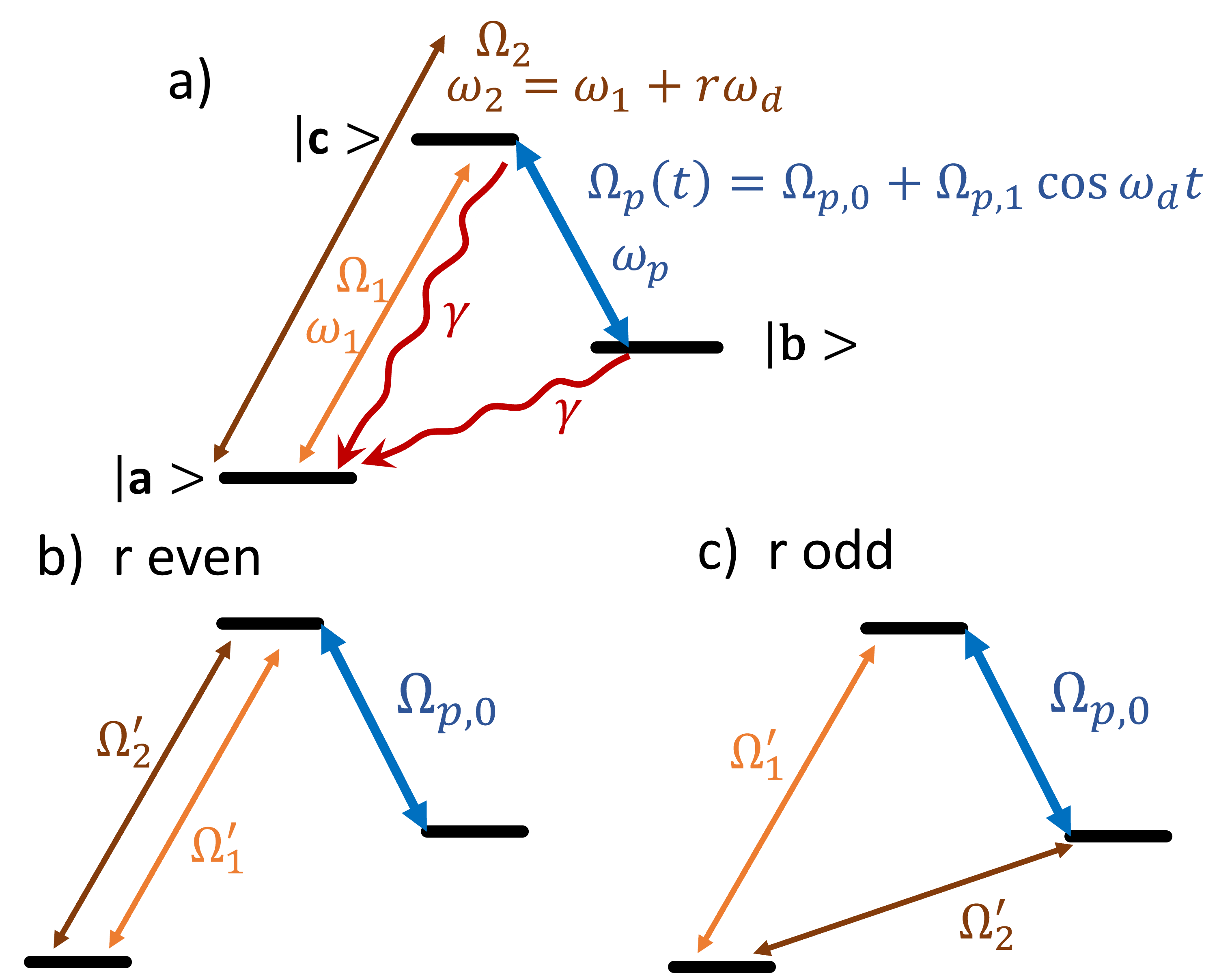
Refer to caption
Figure 4: (a) Sketch of the ac-driven lambda system. The levels |b⟩ket𝑏\left|b\right> and |c⟩ket𝑐\left|c\right> are connected by a pump field with frequency ωpsubscript𝜔p\omega_{\text{p}} and ac-modulated Rabi frequency Ωp​(t)=Ωp,0+Ωp,1​cos⁡ωd​tsubscriptΩp𝑡subscriptΩp0subscriptΩp1subscript𝜔d𝑡\Omega_{\text{p}}(t)=\Omega_{\text{p},0}+\Omega_{\text{p},1}\cos\omega_{\text{d}}t. The signal field frequencies ω1subscript𝜔1\omega_{1} and ω2subscript𝜔2\omega_{2} differ by r𝑟r times the driving frequency ωdsubscript𝜔d\omega_{\text{d}}, i.e., ω2−ω1=r​ωdsubscript𝜔2subscript𝜔1𝑟subscript𝜔d\omega_{2}-\omega_{1}=r\omega_{\text{d}}. (b) For r𝑟r even, the signal Rabi frequency is effectively renormalized. (c) For r𝑟r odd, the coupling structure is changed to a triangular one, which is dipole forbidden in atomic systems for unpumped systems.

The ac-driven lambda system considered here consists of three energy levels coupled by three different coherent fields as sketched in Fig. 4(a). The states |a⟩ket𝑎\left|a\right> and |c⟩ket𝑐\left|c\right> are coupled by two coherent signal fields with frequencies ω1subscript𝜔1\omega_{1} and ω2subscript𝜔2\omega_{2}, respectively. For simplicity we assume that the corresponding Rabi frequencies are equal Ω1=Ω2=ΩssubscriptΩ1subscriptΩ2subscriptΩs\Omega_{1}=\Omega_{2}=\Omega_{\text{s}}. The transition |b⟩↔|c⟩↔ket𝑏ket𝑐\left|b\right>\leftrightarrow\left|c\right> is driven by a pump field with frequency ωpsubscript𝜔p\omega_{\text{p}}. Its Rabi frequency is periodically modulated as

Ωp​(t)=Ωp,0+Ωp,1​cos⁡(ωd​t)subscriptΩp𝑡subscriptΩp0subscriptΩp1subscript𝜔d𝑡\Omega_{\text{p}}(t)=\Omega_{\text{p},0}+\Omega_{\text{p},1}\cos\left(\omega_{\text{d}}t\right) (45)

with dc component Ωp,0subscriptΩp0\Omega_{\text{p},0}, driving amplitude Ωp,1subscriptΩp1\Omega_{\text{p},1} and driving frequency ωdsubscript𝜔d\omega_{\text{d}}. This driving protocol can be experimentally implemented using concatenated driving [58]. Moreover, we impose the frequency matching condition

ω2−ω1=r​ωdsubscript𝜔2subscript𝜔1𝑟subscript𝜔d\omega_{2}-\omega_{1}=r\omega_{\text{d}} (46)

for integer r𝑟r to establish a resonant transition between the two signal fields.

The equation of motion of the generalized density matrix in Eq. (10) including the counting fields reads as

dd​t​ρL𝑑𝑑𝑡subscript𝜌L\displaystyle\frac{d}{dt}\rho_{\text{L}} =\displaystyle= −i​H𝝌​(t)​ρL+i​ρL​H𝟎​(t)𝑖subscript𝐻𝝌𝑡subscript𝜌L𝑖subscript𝜌Lsubscript𝐻0𝑡\displaystyle-iH_{\boldsymbol{\chi}}(t)\rho_{\text{L}}+i\rho_{\text{L}}H_{\boldsymbol{0}}(t) (47)
+γ​D​[|a⟩​⟨b|]​ρL+γ​D​[|a⟩​⟨c|]​ρL,𝛾𝐷delimited-[]ket𝑎bra𝑏subscript𝜌L𝛾𝐷delimited-[]ket𝑎bra𝑐subscript𝜌L\displaystyle+\gamma D\left[\left|a\right>\left<b\right|\right]\rho_{\text{L}}+\gamma D\left[\left|a\right>\left<c\right|\right]\rho_{\text{L}},

where we have added two dissipators describing the incoherent relaxation from the states |b⟩ket𝑏\left|b\right> and |c⟩ket𝑐\left|c\right> to state |a⟩ket𝑎\left|a\right>. For simplicity, we have assumed that both processes have equal relaxation constants γ𝛾\gamma. The counting field of the incoherent processes has been omitted. The semiclassical Hamiltonian reads

H𝝌​(t)subscript𝐻𝝌𝑡\displaystyle H_{\boldsymbol{\chi}}(t) =\displaystyle= ∑α=a,b,cϵα​|α⟩​⟨α|+Ωp​(t)2​(e−i​ωp​t​|c⟩​⟨b|+ h.c.)subscript𝛼𝑎𝑏𝑐subscriptitalic-ϵ𝛼ket𝛼bra𝛼subscriptΩp𝑡2superscript𝑒𝑖subscript𝜔p𝑡ket𝑐bra𝑏 h.c.\displaystyle\sum_{\alpha=a,b,c}\epsilon_{\alpha}\left|\alpha\right>\left<\alpha\right|+\frac{\Omega_{\text{p}}(t)}{2}\left(e^{-i\omega_{\text{p}}t}\left|c\right>\left<b\right|+\text{ h.c.}\right)
+\displaystyle+ [(Ω12​ei​χ1−i​ω1​t+Ω22​ei​χ2−i​ω2​t)​|c⟩​⟨a|+ h.c.].delimited-[]subscriptΩ12superscript𝑒𝑖subscript𝜒1𝑖subscript𝜔1𝑡subscriptΩ22superscript𝑒𝑖subscript𝜒2𝑖subscript𝜔2𝑡ket𝑐bra𝑎 h.c.\displaystyle\left[\left(\frac{\Omega_{1}}{2}e^{i\chi_{1}-i\omega_{1}t}+\frac{\Omega_{2}}{2}e^{i\chi_{2}-i\omega_{2}t}\right)\left|c\right>\left<a\right|+\text{ h.c.}\right].

The photonic dynamics of the system can be numerically calculated along the lines presented in Sec. II.4. The behavior in the stationary is depicted in Figs. 5 and 6, where we observe a sensitive dependence of the photon flux, the fluctuations, and the signal-to-noise ratio as a function of the signal frequency ω1subscript𝜔1\omega_{1} and the driving amplitude Ωp,1subscriptΩp1\Omega_{\text{p},1}. To check the consistency of the FCS and the PRFT predictions, we have compared the number of photons absorbed by the dissipator with the total change of photons in modes k=1𝑘1k=1 and k=2𝑘2k=2 and found a perfect agreement (not shown).

IV.2 Effective treatment

Refer to caption
Figure 5: Photon flux, its fluctuations and the signal-to-noise ratio into the signal field k=2𝑘2k=2 for different resonance orders r=0𝑟0r=0, r=1𝑟1r=1, and r=2𝑟2r=2. The analytical predictions using the cumulant-generating function in Eq. (LABEL:eq:cumulantGeneratingFunctionLambdaSystem) (dashed) are benchmarked against the exact numerical results (solid). Overall parameters are ωd=40​Ωp,0subscript𝜔d40subscriptΩp0\omega_{\text{d}}=40\Omega_{\text{p},0}, Ωp,1=2​ωdsubscriptΩp12subscript𝜔d\Omega_{\text{p},1}=2\omega_{\text{d}}, ϵc=ϵb+ωpsubscriptitalic-ϵ𝑐subscriptitalic-ϵ𝑏subscript𝜔p\epsilon_{c}=\epsilon_{b}+\omega_{\text{p}}, and γ=0.2​Ωp,0𝛾0.2subscriptΩp0\gamma=0.2\Omega_{\text{p},0}.

To obtain a deeper understanding of the underlying physical processes, we derive an analytical expression for the stationary cumulant-generating function in the experimentally relevant limit Ωs≪ϵa,Δ,ϵb,Δ,ϵc,Δ,γ≪ωdformulae-sequencemuch-less-thansubscriptΩssubscriptitalic-ϵ𝑎Δsubscriptitalic-ϵ𝑏Δsubscriptitalic-ϵ𝑐Δmuch-less-than𝛾subscript𝜔d\Omega_{\text{s}}\ll\epsilon_{a,\Delta},\epsilon_{b,\Delta},\epsilon_{c,\Delta},\gamma\ll\omega_{\text{d}}, where ϵa,Δ=ϵasubscriptitalic-ϵ𝑎Δsubscriptitalic-ϵ𝑎\epsilon_{a,\Delta}=\epsilon_{a}, ϵb,Δ=ϵb+ωp−ω1subscriptitalic-ϵ𝑏Δsubscriptitalic-ϵ𝑏subscript𝜔psubscript𝜔1\epsilon_{b,\Delta}=\epsilon_{b}+\omega_{\text{p}}-\omega_{1}, ϵc,Δ=ϵc−ω1subscriptitalic-ϵ𝑐Δsubscriptitalic-ϵ𝑐subscript𝜔1\epsilon_{c,\Delta}=\epsilon_{c}-\omega_{1}. To this end, we first transform Eq. (47) into a rotating frame defined by

Urot​(t)subscript𝑈rot𝑡\displaystyle U_{\text{rot}}(t) =\displaystyle= exp⁡[−i​Ωp,12​ωd​sin⁡(ωd​t)​(|b⟩​⟨c|+|c⟩​⟨b|)]𝑖subscriptΩp12subscript𝜔dsubscript𝜔d𝑡ket𝑏bra𝑐ket𝑐bra𝑏\displaystyle\exp\left[-i\frac{\Omega_{\text{p},1}}{2\omega_{\text{d}}}\sin(\omega_{\text{d}}t)\left(\left|b\right>\left<c\right|+\left|c\right>\left<b\right|\right)\right] (49)

and apply then a rotating-wave approximation following Refs. [59, 60]. In doing so, the dissipator in Eq. (47) remains unchanged, and we obtain an effective time-independent Hamiltonian

H𝝌subscript𝐻𝝌\displaystyle H_{\boldsymbol{\chi}} =\displaystyle= ϵa,Δ​|a⟩​⟨a|+ϵb,Δ+ϵc,Δ2​(|b⟩​⟨b|+|c⟩​⟨c|)subscriptitalic-ϵ𝑎Δket𝑎bra𝑎subscriptitalic-ϵ𝑏Δsubscriptitalic-ϵ𝑐Δ2ket𝑏bra𝑏ket𝑐bra𝑐\displaystyle\epsilon_{a,\Delta}\left|a\right>\left<a\right|+\frac{\epsilon_{b,\Delta}+\epsilon_{c,\Delta}}{2}\left(\left|b\right>\left<b\right|+\left|c\right>\left<c\right|\right) (50)
+\displaystyle+ 𝒥0​(Ωp,1ωd)​ϵb,Δ−ϵc,Δ2​[|b⟩​⟨b|−|c⟩​⟨c|]subscript𝒥0subscriptΩ𝑝1subscript𝜔dsubscriptitalic-ϵ𝑏Δsubscriptitalic-ϵ𝑐Δ2delimited-[]ket𝑏bra𝑏ket𝑐bra𝑐\displaystyle\mathcal{J}_{0}\left(\frac{\Omega_{p,1}}{\omega_{\text{d}}}\right)\frac{\epsilon_{b,\Delta}-\epsilon_{c,\Delta}}{2}\left[\left|b\right>\left<b\right|-\left|c\right>\left<c\right|\right]
+\displaystyle+ Ωp,02​(|b⟩​⟨c|+|c⟩​⟨b|)subscriptΩp02ket𝑏bra𝑐ket𝑐bra𝑏\displaystyle\frac{\Omega_{\text{p},0}}{2}\left(\left|b\right>\left<c\right|+\left|c\right>\left<b\right|\right)
+\displaystyle+ Hsig(r),superscriptsubscript𝐻sig𝑟\displaystyle H_{\text{sig}}^{(r)},

where 𝒥r​(x)subscript𝒥𝑟𝑥\mathcal{J}_{r}\left(x\right) denotes the r𝑟r-th order Bessel function of the first kind. Interestingly, the structure of the Hamiltonian Hsig(r)superscriptsubscript𝐻sig𝑟H_{\text{sig}}^{(r)} describing the transitions induced by the signal fields depends on the parity of the order r𝑟r. For r𝑟r even, the signal-field Hamiltonian

Hsig(r)superscriptsubscript𝐻sig𝑟\displaystyle H_{\text{sig}}^{(r)} =\displaystyle= Ωs​[e−i​χ1​𝒥0​(Ωp,12​ωd)​|c⟩​⟨a|+h.c.]subscriptΩsdelimited-[]superscript𝑒𝑖subscript𝜒1subscript𝒥0subscriptΩp12subscript𝜔dket𝑐bra𝑎h.c.\displaystyle\Omega_{\text{s}}\left[e^{-i\chi_{1}}\mathcal{J}_{0}\left(\frac{\Omega_{\text{p},1}}{2\omega_{\text{d}}}\right)\left|c\right>\left<a\right|+\text{h.c.}\right] (51)
+\displaystyle+ Ωs​[e−i​χ2​𝒥r​(Ωp,12​ωd)​|c⟩​⟨a|+h.c.]subscriptΩsdelimited-[]superscript𝑒𝑖subscript𝜒2subscript𝒥𝑟subscriptΩp12subscript𝜔dket𝑐bra𝑎h.c.\displaystyle\Omega_{\text{s}}\left[e^{-i\chi_{2}}\mathcal{J}_{r}\left(\frac{\Omega_{\text{p},1}}{2\omega_{\text{d}}}\right)\left|c\right>\left<a\right|+\text{h.c.}\right]

is a renormalized version of the original transition terms. Yet, for r𝑟r odd, the signal-field Hamiltonian

Hsig(r)superscriptsubscript𝐻sig𝑟\displaystyle H_{\text{sig}}^{(r)} =\displaystyle= Ωs​[e−i​χ1​𝒥0​(Ωp,12​ωd)​|c⟩​⟨a|+h.c.]subscriptΩsdelimited-[]superscript𝑒𝑖subscript𝜒1subscript𝒥0subscriptΩp12subscript𝜔dket𝑐bra𝑎h.c.\displaystyle\Omega_{\text{s}}\left[e^{-i\chi_{1}}\mathcal{J}_{0}\left(\frac{\Omega_{\text{p},1}}{2\omega_{\text{d}}}\right)\left|c\right>\left<a\right|+\text{h.c.}\right] (52)
+\displaystyle+ Ωs​[e−i​χ2​𝒥r​(Ωp,12​ωd)​|b⟩​⟨a|+h.c.]subscriptΩsdelimited-[]superscript𝑒𝑖subscript𝜒2subscript𝒥𝑟subscriptΩp12subscript𝜔dket𝑏bra𝑎h.c.\displaystyle\Omega_{\text{s}}\left[e^{-i\chi_{2}}\mathcal{J}_{r}\left(\frac{\Omega_{\text{p},1}}{2\omega_{\text{d}}}\right)\left|b\right>\left<a\right|+\text{h.c.}\right]

exhibits an additional transition between levels a↔b↔𝑎𝑏a\leftrightarrow b, establishing a triangular structure as sketched in Fig. 4(c). Intriguingly, as such a triangular structure is dipole-forbidden in atomic systems, the ac-driving protocol provides a way to circumvent this selection rule: Selection rules appear due to spatial symmetries of the probed system, e.g., isotropy for atoms. The periodic driving glorifies these spatial symmetries to time-spatial symmetries, which is reflected in the modification of optical selection rules [20] as observed in the lambda system in Fig. 4.

As shown in detail in Appendix D.1, the counting-field dependent eigenvalue λ0;χsubscript𝜆0𝜒\lambda_{0;\mathbf{\chi}} determining the asymptotic moment-generating function in Eq. (24) can be evaluated using second-order perturbation theory for non-Hermitian systems. For the case ϵc−ϵb=ωpsubscriptitalic-ϵ𝑐subscriptitalic-ϵ𝑏subscript𝜔p\epsilon_{c}-\epsilon_{b}=\omega_{\text{p}}, we obtain

λ0;𝝌subscript𝜆0𝝌\displaystyle\lambda_{0;\boldsymbol{\chi}} =\displaystyle= ∑α=b,cΩα,𝝌​[−Ωα,𝝌∗+Ωα,𝟎∗]​1i​ϵ~α−γsubscript𝛼𝑏𝑐subscriptΩ𝛼𝝌delimited-[]superscriptsubscriptΩ𝛼𝝌superscriptsubscriptΩ𝛼01𝑖subscript~italic-ϵ𝛼𝛾\displaystyle\sum_{\alpha=b,c}\Omega_{\alpha,\boldsymbol{\chi}}\left[-\Omega_{\alpha,\boldsymbol{\chi}}^{*}+\Omega_{\alpha,\boldsymbol{0}}^{*}\right]\frac{1}{i\tilde{\epsilon}_{\alpha}-\gamma}
+\displaystyle+ ∑α=b,cΩα,0∗​[−Ωα,𝟎+Ωα,𝝌]​1−i​ϵ~α−γ+𝒪​(Ωs3),subscript𝛼𝑏𝑐superscriptsubscriptΩ𝛼0delimited-[]subscriptΩ𝛼0subscriptΩ𝛼𝝌1𝑖subscript~italic-ϵ𝛼𝛾𝒪superscriptsubscriptΩs3\displaystyle\sum_{\alpha=b,c}\Omega_{\alpha,0}^{*}\left[-\Omega_{\alpha,\boldsymbol{0}}+\Omega_{\alpha,\boldsymbol{\chi}}\right]\frac{1}{-i\tilde{\epsilon}_{\alpha}-\gamma}+\mathcal{O}\left(\Omega_{\text{s}}^{3}\right),

where

Ωb,𝝌subscriptΩ𝑏𝝌\displaystyle\Omega_{b,\boldsymbol{\chi}} =\displaystyle= Ωs2​[e−i​χ1​𝒥0​(Ωp,12​ωd)+e−i​χ2+i​r​π​𝒥r​(Ωp,12​ωd)],subscriptΩs2delimited-[]superscript𝑒𝑖subscript𝜒1subscript𝒥0subscriptΩp12subscript𝜔dsuperscript𝑒𝑖subscript𝜒2𝑖𝑟𝜋subscript𝒥𝑟subscriptΩp12subscript𝜔d\displaystyle\frac{\Omega_{\text{s}}}{\sqrt{2}}\left[e^{-i\chi_{1}}\mathcal{J}_{0}\left(\frac{\Omega_{\text{p},1}}{2\omega_{\text{d}}}\right)+e^{-i\chi_{2}+ir\pi}\mathcal{J}_{r}\left(\frac{\Omega_{\text{p},1}}{2\omega_{\text{d}}}\right)\right],
Ωc,𝝌subscriptΩ𝑐𝝌\displaystyle\Omega_{c,\boldsymbol{\chi}} =\displaystyle= Ωs2​[e−i​χ1​𝒥0​(Ωp,12​ωd)+e−i​χ2​𝒥r​(Ωp,12​ωd)].subscriptΩs2delimited-[]superscript𝑒𝑖subscript𝜒1subscript𝒥0subscriptΩp12subscript𝜔dsuperscript𝑒𝑖subscript𝜒2subscript𝒥𝑟subscriptΩ𝑝12subscript𝜔d\displaystyle\frac{\Omega_{\text{s}}}{\sqrt{2}}\left[e^{-i\chi_{1}}\mathcal{J}_{0}\left(\frac{\Omega_{\text{p},1}}{2\omega_{\text{d}}}\right)+e^{-i\chi_{2}}\mathcal{J}_{r}\left(\frac{\Omega_{p,1}}{2\omega_{\text{d}}}\right)\right].

Moreover, ϵ~b=ϵb−ω1−Ωp,0subscript~italic-ϵ𝑏subscriptitalic-ϵ𝑏subscript𝜔1subscriptΩp0\tilde{\epsilon}_{b}=\epsilon_{b}-\omega_{1}-\Omega_{\text{p},0} and ϵ~c=ϵc−ω1+Ωp,0subscript~italic-ϵ𝑐subscriptitalic-ϵ𝑐subscript𝜔1subscriptΩp0\tilde{\epsilon}_{c}=\epsilon_{c}-\omega_{1}+\Omega_{\text{p},0} are two of the quasienergies of the closed system for Ωs=0subscriptΩs0\Omega_{\text{s}}=0. In Fig. 5 we benchmark the analytical calculation for three orders r=0,1,2𝑟012r=0,1,2 and find a perfect agreement.

IV.3 Discussion

Refer to caption
Figure 6: Analysis of the photon flux from signal field k=1𝑘1k=1 into the signal field k=2𝑘2k=2 as a function of driving amplitude for the three resonance orders n=0,1,2𝑛012n=0,1,2. Overall parameters are the same as in Fig. 5.

Here we discuss the lambda system for a possible application as a frequency up-conversion device, which converts photons from mode k=1𝑘1k=1 to mode k=2𝑘2k=2. To this end, we seek for combinations of the detuning ωΔ=ϵc−ω1subscript𝜔Δsubscriptitalic-ϵ𝑐subscript𝜔1\omega_{\Delta}=\epsilon_{c}-\omega_{1} and driving amplitude Ωp,1subscriptΩp1\Omega_{\text{p},1} with a significant photon flux I2subscript𝐼2I_{2}, while exhibiting a high signal-to-noise ratio I2/σI,2subscript𝐼2subscript𝜎𝐼2I_{2}/\sigma_{I,2}.

Detuning. Figure 5 investigates the photon transport for a driving amplitude Ωp,1=2​ωdsubscriptΩp12subscript𝜔d\Omega_{\text{p},1}=2\omega_{\text{d}}. In all orders r𝑟r, the photon flux shows two resonances located at the energies of the Rabi splitting ωΔ=±Ωp,0subscript𝜔Δplus-or-minussubscriptΩp0\omega_{\Delta}=\pm\Omega_{\text{p},0}. Close to the two resonance peaks, the flux is negative, as net absorption due to the dissipation dominates over the coherent energy flux. Accordingly, the noise is significantly enhanced. Away from the resonances, the photon flux can be positive, meaning photons are being pumped from field k=1𝑘1k=1 to field k=2𝑘2k=2 via the assistance of the pump field.

The signal-to-noise ratio is particularly high for a large negative detuning ωΔ≪−Ωp,0much-less-thansubscript𝜔ΔsubscriptΩp0\omega_{\Delta}\ll-\Omega_{\text{p},0} for the resonances r=0𝑟0r=0 and r=2𝑟2r=2, and around ωΔ≈0subscript𝜔Δ0\omega_{\Delta}\approx 0 for the resonance order r=1𝑟1r=1. In the former cases, the detuning suppresses the absorption of photons, while in the latter case, the absorption is partly suppressed by a destructive interference known as electromagnetically-induced transparency [61].

Driving amplitude. In Fig. 6, we investigate the photon transport for a negative detuning ωΔ=−2​Ωp,0subscript𝜔Δ2subscriptΩp0\omega_{\Delta}=-2\Omega_{\text{p},0}. Qualitatively similar observation can be found for ωΔ=0subscript𝜔Δ0\omega_{\Delta}=0 (not shown). The photon flux I2subscript𝐼2I_{2} is always positive for r=0𝑟0r=0 because of the chosen signal phases φ1−φ2=π/2subscript𝜑1subscript𝜑2𝜋2\varphi_{1}-\varphi_{2}=\pi/2, resembling the photon transport in the two-level system of Sec. III. Contrary, the photon flux can be either positive or negative for the resonance orders r=1,2𝑟12r=1,2. Because of the Bessel functions, the photon flux shows overall an oscillatory dependence on the pump field amplitude. A similar Bessel function dependence can be observed for the fluctuations σI,2subscript𝜎𝐼2\sigma_{I,2}.

At particular values of the driving amplitude Ωp,0subscriptΩp0\Omega_{\text{p},0}, the Bessel function has a root. According to Eqs. (LABEL:eq:cumulantGeneratingFunctionLambdaSystem) and  (LABEL:eq:effectiveRabifrequencies), this leads to vanishing dependence of the eigenvalue λ0;𝝌subscript𝜆0𝝌\lambda_{0;\boldsymbol{\chi}} on either counting field χ1subscript𝜒1\chi_{1} or χ2subscript𝜒2\chi_{2}. As a consequence, the photon flux vanishes completely, meaning that the mean photon flux and all higher cumulants are zero. Thus, the transport into signal mode k=2𝑘2k=2 is completely suppressed and the system becomes transparent for the frequency ω2subscript𝜔2\omega_{2}. This effect is coined coherent destruction of tunneling, and has been identified in various contexts, such as electronic transport [62], many-body dynamics in interacting systems [63, 60, 59], and topological band structures [64]. In the present context, the coherent-destruction of tunneling suppresses the Josephson flux between two photonic modes due to the control of the pump field.

From Fig. 6 we can determine a driving amplitude for which the signal-to-noise ratio is very high, i.e., where the lambda system can be deployed as a frequency upconversion device. The figure suggests to use the r=2𝑟2r=2 resonance around Ωp,1≈ωdsubscriptΩp1subscript𝜔d\Omega_{\text{p},1}\approx\omega_{\text{d}} or the r=1𝑟1r=1 resonance around Ωp,1≈3.5​ωdsubscriptΩp13.5subscript𝜔𝑑\Omega_{\text{p},1}\approx 3.5\omega_{d}. Both parameter combinations feature a significant photon flux I2subscript𝐼2I_{2} while the fluctuations are relatively small. We note that the jump in the r=1𝑟1r=1 signal-to-noise ratio appears as I2subscript𝐼2I_{2} changes from positive to negative at the same point where the fluctuations hit a zero.

V Conclusions and outlook

In this paper, we have developed a framework unifying the standard FCS and the recently developed PRFT. To this end, we have defined a moment-generating function that reduces to the FCS and the PRFT in the respective limits. Importantly, the unified framework is non-perturbative in all parameters and paves thus the way to a non-perturbative spectroscopic framework, that allows the development of metrological methods which can characterize the probability distribution of stimulated processes.

The framework has been applied to the multimode Jaynes-Cummings model, where two modes coherently drive a two-level system, that is additionally coupled to a continuum of incoherent photon modes. We have found that the unified cumulant-generating function consistently describes the photon statistics of coherent and incoherent emission. Moreover, we have found that the light-matter entanglement predicted by the PRFT in the closed quantum systems leads to diverging transport fluctuations in the dissipative system. These fluctuations should be observable in spectroscopic experiments, which we will discuss in a future work.

As a more sophisticated application, we have investigated an ac-driven lambda system for its application as a frequency-conversion device. In doing so, we have found that the ac-driving can create a triangular coupling structure, which is actually electrically-dipole forbidden in atoms. Using our unified framework, we could identify parameters that feature both a significant photon conversion and a high signal-to-noise ratio.

The calculations in this paper could be carried out analytically. To this end, we took advantage of the method of the truncated characteristic polynomial. In the weak driving regime, we have generalized the common stationary perturbation theory known for Hermitian systems, to non-Hermitian ones. As an alternative method, one can reduce the dimension of the Liouvillian equation by means of adiabatic elimination. Depending on the system, either method will be more suitable. For more sophisticated models, efficient numerical evaluation can be easily implemented. Besides, the polynomial perturbation theory can be applied even for larger systems if the system parameters are on different orders of magnitude [65].

To derive a quantum master equation for the multi-mode Jaynes-Cummings model, we have applied the quantum Langevin formalism. The application of more advanced methods such as the hierarchy equations of motion or the polaron transformation is likewise possible and can lead to new insights into fundamental concepts of light-matter interactions. Using the modified FCS in the hierarchy equations of motion in Ref. [17], it is also possible to investigate the energy conservation within the PRFT for open quantum systems, which do not feature an excitation number conservation as the Jaynes-Cummings model considered here. The PRFT can also give rise to the development of new spectroscopic and metrological methods, which help to improve detection protocols for electric fields [66, 67] and dark matter  [28, 29, 68]. Moreover, the unified framework introduced here can find application to heat engines and quantum batteries.

In the present work, the PRFT has been formally investigated in the context of cavity quantum electrodynamics, while the application to spectroscopic setups, where a propagating laser field drives a quantum system, will be considered in future work. The flexibility of the PRFT will thereby allow to spectroscopically describe complex many-body systems of interacting quantum emitters, such as arrays of Rydberg atoms, which can exhibit a pronounced photonic non-linearity [69, 70, 71]. Other possible spectroscopic application are higher-harmonic generation [72] and spectroscopy with non-classical light [73, 74].

Acknowledgments

G.E. acknowledges the support by the Guangdong Provincial Key Laboratory (Grant No.2019B121203002) J.Y. L. acknowledges the support from the National Natural Science Foundation of China (Grant Nos. 11774311). V. M. B. wish to thank NTT Research for their financial and technical support. G.P. acknowledges the Spanish Ministry of Economy and Competitiveness for financial support through the grant: PID2020-117787GBI00 and support from CSIC Interdisciplinary Thematic Platform on Quantum Technologies (PTI-QTEP+)

Appendix A Unification of standard FCS and PRFT

In the following, we explain the concepts of the standard FCS and the PRFT and how to combine them into a unified framework. The standard FCS and the PRFT are constructed in terms of two-point protective and two-point tomographic measurements, respectively, which leads to different interpretations of the probability distributions and their cumulants. A detailed discussion on this issue can be found in Ref. [16]. We refer to Sec. II for the explanations about the system and notation.

A.1 Standard FCS

The standard FCS considers the probability distribution p𝒏1∣𝒏0subscript𝑝conditionalsubscript𝒏1subscript𝒏0p_{\boldsymbol{n}_{1}\mid\boldsymbol{n}_{0}} quantifying the probability that there are 𝒏1subscript𝒏1\boldsymbol{n}_{1} photons in the incoherent modes a^ksubscript^𝑎𝑘\hat{a}_{k} with k∈{ND,…,ND+NB }𝑘subscript𝑁D…subscript𝑁Dsubscript𝑁B k\in\{N_{\text{D}},\dots,N_{\text{D}}+N_{\text{\text{B} }}\} at time t>0𝑡0t>0 given that there have been 𝒏0subscript𝒏0\boldsymbol{n}_{0} photons at time t=0𝑡0t=0. The mean change of photons in that mode can be determined by the probability distribution

p𝒎subscript𝑝𝒎\displaystyle p_{\boldsymbol{m}} ≡\displaystyle\equiv ∑𝒏0p𝒏0+𝒎∣𝒏0​(t)​p𝒏0​(0)subscriptsubscript𝒏0subscript𝑝subscript𝒏0conditional𝒎subscript𝒏0𝑡subscript𝑝subscript𝒏00\displaystyle\sum_{\boldsymbol{n}_{0}}p_{\boldsymbol{n}_{0}+\boldsymbol{m}\mid\boldsymbol{n}_{0}}(t)p_{\boldsymbol{n}_{0}}(0) (55)
=\displaystyle= 1(2​π)NB​∫−ππ𝑑𝝃NB​ei​𝝃⋅𝒎​M𝝃(FCS)​(t),1superscript2𝜋subscript𝑁𝐵superscriptsubscript𝜋𝜋differential-dsuperscript𝝃subscript𝑁𝐵superscript𝑒⋅𝑖𝝃𝒎superscriptsubscript𝑀𝝃FCS𝑡\displaystyle\frac{1}{(2\pi)^{N_{B}}}\int_{-\pi}^{\pi}d\boldsymbol{\xi}^{N_{B}}e^{i\boldsymbol{\xi}\cdot\boldsymbol{m}}M_{\boldsymbol{\xi}}^{(\text{FCS})}(t),

where in the second line we have introduced the moment-generating function

M𝝃(FCS)​(t)superscriptsubscript𝑀𝝃FCS𝑡\displaystyle M_{\boldsymbol{\xi}}^{(\text{FCS})}(t) =\displaystyle=  tr​[U^𝝃/2​(t)​∑𝒏0[P^𝒏0​ρ​(0)​P^𝒏0]​U^−𝝃/2†​(t)]. trdelimited-[]subscript^𝑈𝝃2𝑡subscriptsubscript𝒏0delimited-[]subscript^𝑃subscript𝒏0𝜌0subscript^𝑃subscript𝒏0superscriptsubscript^𝑈𝝃2†𝑡\displaystyle\text{ tr}\left[\hat{U}_{\boldsymbol{\xi}/2}(t)\sum_{\boldsymbol{n}_{0}}\left[\hat{P}_{\boldsymbol{n}_{0}}\rho(0)\hat{P}_{\boldsymbol{n}_{0}}\right]\hat{U}_{-\boldsymbol{\xi}/2}^{\dagger}(t)\right].

Here, U^𝝃​(t)subscript^𝑈𝝃𝑡\hat{U}_{\boldsymbol{\xi}}(t) denotes the generalized time-evolution operator defined in Eq. (6) with 𝝌=𝟎𝝌0\boldsymbol{\chi}=\boldsymbol{0}, and P^𝒏0=|𝒏0⟩​⟨𝒏0|subscript^𝑃subscript𝒏0ketsubscript𝒏0brasubscript𝒏0\hat{P}_{\boldsymbol{n}_{0}}=\left|\boldsymbol{n}_{0}\right>\left<\boldsymbol{n}_{0}\right| denotes the projector on the number basis of the incoherent photon modes. As by assumption [P^𝒏0,ρ​(0)]=0subscript^𝑃subscript𝒏0𝜌00\left[\hat{P}_{\boldsymbol{n}_{0}},\rho(0)\right]=0, the projectors can be neglected.

A.2 PRFT in an isolated quantum system

For a photonic mode in a coherent state, the projection in Eq. (LABEL:eq:momentGeneratingFktFCS) would destroy the coherences in the number basis, prohibiting the correct counting of photons by the moment-generating function in Eq. (LABEL:eq:momentGeneratingFktFCS). The PRFT maintains the coherent initial state by replacing the initial projective measurement at time t=0𝑡0t=0 by a tomographic measurement [16]. The PRFT predicts the probability distribution p𝒏subscript𝑝𝒏p_{\boldsymbol{n}} that the coherent photon modes a^ksubscript^𝑎𝑘\hat{a}_{k} with k∈{1,…,ND}𝑘1…subscript𝑁𝐷k\in\{1,\dots,N_{D}\} contain 𝒏𝒏\boldsymbol{n} photons.

The photonic probabilities can be calculated via an inverse Fourier transformation of the moment-generating function

p𝒏​(t)subscript𝑝𝒏𝑡\displaystyle p_{\boldsymbol{n}}(t) =\displaystyle= 1(2​π)ND​∫−ππ𝑑𝝌ND​ei​𝝌⋅𝒏​M𝝌(PRFT)​(t),1superscript2𝜋subscript𝑁Dsuperscriptsubscript𝜋𝜋differential-dsuperscript𝝌subscript𝑁Dsuperscript𝑒⋅𝑖𝝌𝒏superscriptsubscript𝑀𝝌PRFT𝑡\displaystyle\frac{1}{(2\pi)^{N_{\text{D}}}}\int_{-\pi}^{\pi}d\boldsymbol{\chi}^{N_{\text{D}}}e^{i\boldsymbol{\chi}\cdot\boldsymbol{n}}M_{\boldsymbol{\chi}}^{(\text{PRFT})}(t), (57)

where

M𝝌(PRFT)​(t)superscriptsubscript𝑀𝝌PRFT𝑡\displaystyle M_{\boldsymbol{\chi}}^{(\text{PRFT})}(t) ≡\displaystyle\equiv tr​[e−i​𝝌⋅𝒏^D​ρ​(t)]trdelimited-[]superscript𝑒⋅𝑖𝝌subscript^𝒏D𝜌𝑡\displaystyle\text{tr}\left[e^{-i\boldsymbol{\chi}\cdot\hat{\boldsymbol{n}}_{\text{D}}}\rho(t)\right]
=\displaystyle= 12​tr​[U^𝝌​(t)​e−i​𝝌⋅𝒏^D​ρ​(0)​U^𝟎†​(t)]12trdelimited-[]subscript^𝑈𝝌𝑡superscript𝑒⋅𝑖𝝌subscript^𝒏D𝜌0subscriptsuperscript^𝑈†0𝑡\displaystyle\frac{1}{2}\text{tr}\left[\hat{U}_{\boldsymbol{\chi}}(t)e^{-i\boldsymbol{\chi}\cdot\hat{\boldsymbol{n}}_{\text{D}}}\rho(0)\hat{U}^{\dagger}_{\boldsymbol{0}}(t)\right]
+\displaystyle+ 12​tr​[U^𝟎​(t)​ρ​(0)​e−i​𝝌⋅𝒏^D​U^−𝝌†​(t)],12trdelimited-[]subscript^𝑈0𝑡𝜌0superscript𝑒⋅𝑖𝝌subscript^𝒏Dsubscriptsuperscript^𝑈†𝝌𝑡\displaystyle\frac{1}{2}\text{tr}\left[\hat{U}_{\boldsymbol{0}}(t)\rho(0)e^{-i\boldsymbol{\chi}\cdot\hat{\boldsymbol{n}}_{\text{D}}}\hat{U}^{\dagger}_{-\boldsymbol{\chi}}(t)\right],

where U^𝝌​(t)subscript^𝑈𝝌𝑡\hat{U}_{\boldsymbol{\chi}}(t) denotes the generalized time-evolution operator defined in Eq. (6) with 𝝃=0𝝃0\boldsymbol{\xi}=0.

Within the semiclassical framework, the PRFT shows that the moment-generating function can be expressed as

M𝝌(PRFT)​(t)=Mdy,𝝌(PRFT)​(t)​M𝝌(PRFT)​(0).superscriptsubscript𝑀𝝌PRFT𝑡superscriptsubscript𝑀dy𝝌PRFT𝑡superscriptsubscript𝑀𝝌PRFT0M_{\boldsymbol{\chi}}^{(\text{PRFT})}(t)=M_{\text{dy},\boldsymbol{\chi}}^{(\text{PRFT})}(t)M_{\boldsymbol{\chi}}^{(\text{PRFT})}(0). (59)

Thereby, we have introduced the dynamical moment-generating function

Mdy,𝝌(PRFT)​(t)=12​tr​[𝒰^𝟎†​(t)​𝒰^𝝌​(t)​ρ​(0)+𝒰^−𝝌†​(t)​𝒰^𝟎​(t)​ρ​(0)]superscriptsubscript𝑀dy𝝌PRFT𝑡12trdelimited-[]superscriptsubscript^𝒰0†𝑡subscript^𝒰𝝌𝑡𝜌0superscriptsubscript^𝒰𝝌†𝑡subscript^𝒰0𝑡𝜌0\displaystyle M_{\text{dy},\boldsymbol{\chi}}^{(\text{PRFT})}(t)=\frac{1}{2}\text{tr}\left[\hat{\mathcal{U}}_{\boldsymbol{0}}^{\dagger}(t)\hat{\mathcal{U}}_{\boldsymbol{\chi}}(t)\rho(0)+\hat{\mathcal{U}}_{-\boldsymbol{\chi}}^{\dagger}(t)\hat{\mathcal{U}}_{\boldsymbol{0}}(t)\rho(0)\right]

with 𝒰𝝌†​(t)superscriptsubscript𝒰𝝌†𝑡\mathcal{U}_{\boldsymbol{\chi}}^{\dagger}(t) being the generalized time-evolution operator which describes the dynamics determined by the semiclassical Hamiltonian in Eq. (12):

𝒰^𝝌​(t)=𝒯​exp⁡[−i​∫0tℋ^𝝌​(t′)​𝑑t′],subscript^𝒰𝝌𝑡𝒯𝑖superscriptsubscript0𝑡subscript^ℋ𝝌superscript𝑡′differential-dsuperscript𝑡′\hat{\mathcal{U}}_{\boldsymbol{\chi}}(t)=\mathcal{T}\exp\left[-i\int_{0}^{t}\hat{\mathcal{H}}_{\boldsymbol{\chi}}(t^{\prime})dt^{\prime}\right], (61)

where 𝒯𝒯\mathcal{T} denotes the time-ordering operator. The initial probability distribution p𝒏​(0)subscript𝑝𝒏0p_{\boldsymbol{n}}(0) determines the moment-generating function at time t=0𝑡0t=0, i.e., M𝝌(PRFT)​(0)=∑𝒏p𝒏​(0)​e−i​𝝌⋅𝒏superscriptsubscript𝑀𝝌PRFT0subscript𝒏subscript𝑝𝒏0superscript𝑒⋅𝑖𝝌𝒏M_{\boldsymbol{\chi}}^{(\text{PRFT})}(0)=\sum_{\boldsymbol{n}}p_{\boldsymbol{n}}(0)e^{-i\boldsymbol{\chi}\cdot\boldsymbol{n}} and can be calculated via Eq. (17).

A.3 Combining FCS and PRFT

It is not hard to see that the unified moment-generating function in Eq. (15) generalizes the FCS and the PRFT: the FCS moment-generating function in Eq. (LABEL:eq:momentGeneratingFktFCS) is a special case of Eq. (15) when setting 𝝌=𝟎𝝌0\boldsymbol{\chi}=\boldsymbol{0}, while the PRFT moment-generating function in Eq. (59) is a special case of Eq. (15) when setting 𝝃=𝟎𝝃0\boldsymbol{\xi}=\boldsymbol{0}.

As the dynamics of Eq. (15) involves a continuum of photon modes and each mode has an infinitesimal Hilbert space, the time-evolution of Eq. (15) cannot be exactly determined in general. For this reason, we solve the dynamics of the reduced density matrix of the matter system in Eq. (10) instead, where we use a semiclassical description of the coherent photon modes. Importantly, the construction of the quantum Langevin approach (see, e.g., Ref. [50, 51]) and the derivations of the PRFT (see Ref. [16]) do not interfere with each other, such that the derivation of the generalized quantum master equation in Eq. (11) is straightforward, yet, lengthy. Crucially, when setting either 𝝌=𝟎𝝌0\boldsymbol{\chi}=\boldsymbol{0} or 𝝃=𝟎𝝃0\boldsymbol{\xi}=\boldsymbol{0}, the moment-generating function in Eq. (15) reduces to the well-known limiting case in the FCS or the PRFT, respectively.

A.4 Error discussion

Finally, we discuss the deviation of the probabilities in the PRFT from the exact probabilities. A basic assumption of the PRFT is that the mean-photon number of the initial photonic state Δ​n¯​(t)Δ¯𝑛𝑡\Delta\overline{n}(t) does only change slightly as compared to the mean photon number n¯¯𝑛\overline{n}, i.e., Δ​n¯​(t)≪n¯much-less-thanΔ¯𝑛𝑡¯𝑛\Delta\overline{n}(t)\ll\overline{n}. This property is easily fulfilled for coherent photonic states with a large mean photon number for short and intermediate evolution times. As the derivation of the PRFT in open quantum systems is a straightforward generalization of the PRFT in closed quantum systems, the error analysis as carried out in Ref. [16] applies also to the open system. Additionally, we have to take into account the coupling to the incoherent photon modes, which implies an additional time constrain for the validity of the PRFT as given in Eq. (32).

Appendix B Evaluation of the cumulants in the long-time limit

In this Appendix, we introduce three different methods which allow to analytically determine information about the photonic probability distributions. The methods are applied in Secs. III and IV to the Jaynes-Cummings model and the ac-driven lambda system for illustration.

B.1 Truncation of the characteristic polynomial

The analytical calculation of the eigenvalues λμ;𝝃,𝝌subscript𝜆𝜇𝝃𝝌\lambda_{\mu;\boldsymbol{\xi},\boldsymbol{\chi}} in Eq. (23) will be impossible for large Liouvillians. Here we introduce a method to non-perturbatively determine low-order cumulants in the long-time limit without depending on the exact eigenvalues of the Liouvillian. We restrict the explanations to a single counting field for simplicity.

In general, the characteristic polynomial of the effective Liovillian can be written as

𝒫χ​(z)=∑j=0Naj​(χ)​zjsubscript𝒫𝜒𝑧superscriptsubscript𝑗0𝑁subscript𝑎𝑗𝜒superscript𝑧𝑗\mathcal{P}_{\chi}(z)=\sum_{j=0}^{N}a_{j}(\chi)z^{j} (62)

with counting-field dependent coefficients aj​(χ)subscript𝑎𝑗𝜒a_{j}(\chi). The roots of this polynomial are the eigenvalues of the Liouvillian. Importantly, a0​(0)=0subscript𝑎000a_{0}(0)=0 such that the μ=0𝜇0\mu=0 root of the polynomial is λ0;0=0subscript𝜆000\lambda_{0;0}=0, reflecting the existence of a stationary state. To determine the photonic cumulants κ(m)​(t)superscript𝜅𝑚𝑡\kappa^{(m)}(t) for long times t→∞→𝑡t\rightarrow\infty, we need to calculate the r𝑟r-th derivatives of the root λ0;χsubscript𝜆0𝜒\lambda_{0;\chi}. To this end, one can use the truncated characteristic polynomial instead of the full one:

𝒫χ(R)​(z)=∑j=0Raj​(χ)​zj,subscriptsuperscript𝒫𝑅𝜒𝑧superscriptsubscript𝑗0𝑅subscript𝑎𝑗𝜒superscript𝑧𝑗\mathcal{P}^{(R)}_{\chi}(z)=\sum_{j=0}^{R}a_{j}(\chi)z^{j}, (63)

with R<N𝑅𝑁R<N. Denoting the corresponding roots by λμ;χ(R)superscriptsubscript𝜆𝜇𝜒𝑅\lambda_{\mu;\chi}^{(R)}, their derivatives fulfill

dmd​(−i​χ)m​λ0;χ=0=dmd​(−i​χ)r​λ0;χ=0(R)superscript𝑑𝑚𝑑superscript𝑖𝜒𝑚subscript𝜆0𝜒0superscript𝑑𝑚𝑑superscript𝑖𝜒𝑟superscriptsubscript𝜆0𝜒0𝑅\frac{d^{m}}{d(-i\chi)^{m}}\lambda_{0;\chi=0}=\frac{d^{m}}{d(-i\chi)^{r}}\lambda_{0;\chi=0}^{(R)} (64)

for R≤m𝑅𝑚R\leq m, which we can harness to exactly calculate low-order cumulants. For instance, the μ=0𝜇0\mu=0 root of the first-order truncated characteristic polynomial reads as

λ0,χ(1)=−a0​(χ)a1​(χ),superscriptsubscript𝜆0𝜒1subscript𝑎0𝜒subscript𝑎1𝜒\displaystyle\lambda_{0,\chi}^{(1)}=-\frac{a_{0}(\chi)}{a_{1}(\chi)}, (65)

such that the first cumulant in the long-time limit is given as

κ(1)​(t)=−Re​1a1​(0)​d​a0​(χ)d​(−i​χ)|χ=0​t.superscript𝜅1𝑡evaluated-atRe1subscript𝑎10𝑑subscript𝑎0𝜒𝑑𝑖𝜒𝜒0𝑡\displaystyle\kappa^{(1)}(t)=-\text{Re}\,\frac{1}{a_{1}(0)}\left.\frac{da_{0}(\chi)}{d(-i\chi)}\right|_{\chi=0}t. (66)

Likewise, we find for the second-order truncated eigenvalue

λ0;χ(2)=12​a2​(−a1+a12−4​a0​a2),subscriptsuperscript𝜆20𝜒12subscript𝑎2subscript𝑎1superscriptsubscript𝑎124subscript𝑎0subscript𝑎2\displaystyle\lambda^{(2)}_{0;\chi}=\frac{1}{2a_{2}}\left(-a_{1}+\sqrt{a_{1}^{2}-4a_{0}a_{2}}\right),

where we have suppressed the counting field arguments for a notational reason. Deriving λ0;χ(2)subscriptsuperscript𝜆20𝜒\lambda^{(2)}_{0;\chi} with respect to χ𝜒\chi reproduces the first cumulant in Eq. (66). Evaluation of the second derivative will lead to an unhandy analytical expression, which can be evaluated efficiently with computer algebra systems such as SymPy or Mathematica.

B.2 Stationary perturbation theory in non-Hermitian systems

Here, we generalize the standard stationary perturbation theory from Hermitian systems to non-Hermitian systems. Given the total Liouvillian can be written as

ℒ=ℒ0+g​ℒ1,ℒsubscriptℒ0𝑔subscriptℒ1\mathcal{L}=\mathcal{L}_{0}+g\mathcal{L}_{1}, (68)

where ℒ0subscriptℒ0\mathcal{L}_{0} is the Liouvillian of the unperturbed system, ℒ1subscriptℒ1\mathcal{L}_{1} is the perturbation Liouvillian and 0≤g≪10𝑔much-less-than10\leq g\ll 1 parameterizes the strength of the perturbation.

The goal is to approximatively determine the right and left eigenvectors and their corresponding eigenvalues of the Liouvillian, that are defined by

ℒ​vμℒsubscript𝑣𝜇\displaystyle\mathcal{L}v_{\mu} =\displaystyle= λμ​vμ,subscript𝜆𝜇subscript𝑣𝜇\displaystyle\lambda_{\mu}v_{\mu},
v¯μ​ℒsubscript¯𝑣𝜇ℒ\displaystyle\overline{v}_{\mu}\mathcal{L} =\displaystyle= λμ​v¯μ,subscript𝜆𝜇subscript¯𝑣𝜇\displaystyle\lambda_{\mu}\overline{v}_{\mu}, (69)

respectively. We recall that the eigenvectors corresponding to eigenvalues λμsubscript𝜆𝜇\lambda_{\mu} fulfill the orthogonality relation

⟨v¯μ∣vμ⟩=δk,k′.inner-productsubscript¯𝑣𝜇subscript𝑣𝜇subscript𝛿𝑘superscript𝑘′\left<\overline{v}_{\mu}\mid v_{\mu}\right>=\delta_{k,k^{\prime}}. (70)

The normalization can be achieved by properly rescaling the eigenvectors.

Our aim is to find an expansion of the eigenvalues and eigenvectors in orders of g𝑔g, i.e.,

λμsubscript𝜆𝜇\displaystyle\lambda_{\mu} =\displaystyle= (λμ(0)+g​λμ(1)+g2​λμ(2)+…),superscriptsubscript𝜆𝜇0𝑔superscriptsubscript𝜆𝜇1superscript𝑔2superscriptsubscript𝜆𝜇2…\displaystyle\left(\lambda_{\mu}^{(0)}+g\lambda_{\mu}^{(1)}+g^{2}\lambda_{\mu}^{(2)}+\dots\right),
vμsubscript𝑣𝜇\displaystyle v_{\mu} =\displaystyle= (vμ(0)+g​vμ(1)+g2​vμ(2)+…),superscriptsubscript𝑣𝜇0𝑔superscriptsubscript𝑣𝜇1superscript𝑔2superscriptsubscript𝑣𝜇2…\displaystyle\left(v_{\mu}^{(0)}+gv_{\mu}^{(1)}+g^{2}v_{\mu}^{(2)}+\dots\right),
v¯μsubscript¯𝑣𝜇\displaystyle\overline{v}_{\mu} =\displaystyle= (v¯μ(0)+g​v¯μ(1)+g2​v¯μ(2)+…),superscriptsubscript¯𝑣𝜇0𝑔superscriptsubscript¯𝑣𝜇1superscript𝑔2superscriptsubscript¯𝑣𝜇2…\displaystyle\left(\overline{v}_{\mu}^{(0)}+g\overline{v}_{\mu}^{(1)}+g^{2}\overline{v}_{\mu}^{(2)}+\dots\right), (71)

where we define the unperturbed eigenvalues and eigenstates by

ℒ0​vμ(0)subscriptℒ0superscriptsubscript𝑣𝜇0\displaystyle\mathcal{L}_{0}v_{\mu}^{(0)} =\displaystyle= λμ​vμ(0),subscript𝜆𝜇superscriptsubscript𝑣𝜇0\displaystyle\lambda_{\mu}v_{\mu}^{(0)},
v¯μ(0)​ℒ0superscriptsubscript¯𝑣𝜇0subscriptℒ0\displaystyle\overline{v}_{\mu}^{(0)}\mathcal{L}_{0} =\displaystyle= λμ​v¯μ(0).subscript𝜆𝜇superscriptsubscript¯𝑣𝜇0\displaystyle\lambda_{\mu}\overline{v}_{\mu}^{(0)}. (72)

We want to express g​λμ(n>0)𝑔superscriptsubscript𝜆𝜇𝑛0g\lambda_{\mu}^{(n>0)} and the vμ(n>0),v¯μ(n>0)superscriptsubscript𝑣𝜇𝑛0superscriptsubscript¯𝑣𝜇𝑛0v_{\mu}^{(n>0)},\overline{v}_{\mu}^{(n>0)} in terms of g​λμ(0)𝑔superscriptsubscript𝜆𝜇0g\lambda_{\mu}^{(0)} and the vμ(0),v¯μ(0)superscriptsubscript𝑣𝜇0superscriptsubscript¯𝑣𝜇0v_{\mu}^{(0)},\overline{v}_{\mu}^{(0)}. Inserting these expansions into the right-eigenvector equation in Eq. (69), we find

(ℒ0+g​ℒ1)subscriptℒ0𝑔subscriptℒ1\displaystyle\left(\mathcal{L}_{0}+g\mathcal{L}_{1}\right) (vμ(0)+g​vμ(1)+g2​vμ(2)+…)superscriptsubscript𝑣𝜇0𝑔superscriptsubscript𝑣𝜇1superscript𝑔2superscriptsubscript𝑣𝜇2…\displaystyle\left(v_{\mu}^{(0)}+gv_{\mu}^{(1)}+g^{2}v_{\mu}^{(2)}+\dots\right) (73)
=(λμ(0)+g​λμ(1)+g2​λμ(2)+…)absentsuperscriptsubscript𝜆𝜇0𝑔superscriptsubscript𝜆𝜇1superscript𝑔2superscriptsubscript𝜆𝜇2…\displaystyle=\left(\lambda_{\mu}^{(0)}+g\lambda_{\mu}^{(1)}+g^{2}\lambda_{\mu}^{(2)}+\dots\right)
×(vμ(0)+g​vμ(1)+g2​vμ(2)+…).absentsuperscriptsubscript𝑣𝜇0𝑔superscriptsubscript𝑣𝜇1superscript𝑔2superscriptsubscript𝑣𝜇2…\displaystyle\times\left(v_{\mu}^{(0)}+gv_{\mu}^{(1)}+g^{2}v_{\mu}^{(2)}+\dots\right).

These equations must be fulfilled in all orders of g𝑔g. The zeroth-order is just the unperturbed eigenvalue equation for ℒ0subscriptℒ0\mathcal{L}_{0} in Eq. (72). In first order, we find

ℒ0​vμ(1)+ℒ1​vμ(0)subscriptℒ0superscriptsubscript𝑣𝜇1subscriptℒ1superscriptsubscript𝑣𝜇0\displaystyle\mathcal{L}_{0}v_{\mu}^{(1)}+\mathcal{L}_{1}v_{\mu}^{(0)} =\displaystyle= λμ(1)​vμ(0)+λμ(0)​vμ(1).superscriptsubscript𝜆𝜇1superscriptsubscript𝑣𝜇0superscriptsubscript𝜆𝜇0superscriptsubscript𝑣𝜇1\displaystyle\lambda_{\mu}^{(1)}v_{\mu}^{(0)}+\lambda_{\mu}^{(0)}v_{\mu}^{(1)}. (74)

Multiplying from the left with v¯μ(0)superscriptsubscript¯𝑣𝜇0\overline{v}_{\mu}^{(0)} and using the orthogonality relation in Eq. (70), we readily find the first order correction for the eigenvalue

λμ(1)=⟨v¯μ(0),ℒ1​vμ(0)⟩.superscriptsubscript𝜆𝜇1superscriptsubscript¯𝑣𝜇0subscriptℒ1superscriptsubscript𝑣𝜇0\lambda_{\mu}^{(1)}=\left<\overline{v}_{\mu}^{(0)},\mathcal{L}_{1}v_{\mu}^{(0)}\right>. (75)

To obtain the first-order correction for the related right eigenvector, we expand it as

vμ(1)=∑μ′aμ,μ′​vμ′(0).subscriptsuperscript𝑣1𝜇subscriptsuperscript𝜇′subscript𝑎𝜇superscript𝜇′subscriptsuperscript𝑣0superscript𝜇′v^{(1)}_{\mu}=\sum_{\mu^{\prime}}a_{\mu,\mu^{\prime}}v^{(0)}_{\mu^{\prime}}. (76)

Inserting into Eq. (74), appropriately left-multiplying with v¯μ′≠μ(0)subscriptsuperscript¯𝑣0superscript𝜇′𝜇\overline{v}^{(0)}_{\mu^{\prime}\neq\mu}, and resolving for aμ,μ′subscript𝑎𝜇superscript𝜇′a_{\mu,\mu^{\prime}}, we finally find

vμ(1)=∑μ′⟨v¯k′(0),ℒ1​vμ(0)⟩λμ(0)−λμ′(0)​vμ′(0).subscriptsuperscript𝑣1𝜇subscriptsuperscript𝜇′superscriptsubscript¯𝑣superscript𝑘′0subscriptℒ1superscriptsubscript𝑣𝜇0superscriptsubscript𝜆𝜇0superscriptsubscript𝜆superscript𝜇′0subscriptsuperscript𝑣0superscript𝜇′v^{(1)}_{\mu}=\sum_{\mu^{\prime}}\frac{\left<\overline{v}_{k^{\prime}}^{(0)},\mathcal{L}_{1}v_{\mu}^{(0)}\right>}{\lambda_{\mu}^{(0)}-\lambda_{\mu^{\prime}}^{(0)}}v^{(0)}_{\mu^{\prime}}. (77)

The expression for the left eigenvector can be obtained accordingly. The derivation of the second-order terms can be obtained along the same lines. The second-order eigenvalue equation reads as

ℒ0​vμ(2)+ℒ1​vμ(1)subscriptℒ0superscriptsubscript𝑣𝜇2subscriptℒ1superscriptsubscript𝑣𝜇1\displaystyle\mathcal{L}_{0}v_{\mu}^{(2)}+\mathcal{L}_{1}v_{\mu}^{(1)} =\displaystyle= λμ(2)​vμ(0)+λμ(0)​vμ(2)+λμ(1)​vμ(1).superscriptsubscript𝜆𝜇2superscriptsubscript𝑣𝜇0superscriptsubscript𝜆𝜇0superscriptsubscript𝑣𝜇2superscriptsubscript𝜆𝜇1superscriptsubscript𝑣𝜇1\displaystyle\lambda_{\mu}^{(2)}v_{\mu}^{(0)}+\lambda_{\mu}^{(0)}v_{\mu}^{(2)}+\lambda_{\mu}^{(1)}v_{\mu}^{(1)}.

Multiply from left with v¯μ(0)superscriptsubscript¯𝑣𝜇0\overline{v}_{\mu}^{(0)} and resolving for λμ(2)superscriptsubscript𝜆𝜇2\lambda_{\mu}^{(2)}, we find

λμ(2)=∑k′⟨v¯μ′(0),ℒ1​vμ(0)⟩​⟨v¯k(0),ℒ1​vμ′(0)⟩λμ(0)−λμ′(0).superscriptsubscript𝜆𝜇2subscriptsuperscript𝑘′superscriptsubscript¯𝑣superscript𝜇′0subscriptℒ1superscriptsubscript𝑣𝜇0superscriptsubscript¯𝑣𝑘0subscriptℒ1superscriptsubscript𝑣superscript𝜇′0superscriptsubscript𝜆𝜇0superscriptsubscript𝜆superscript𝜇′0\lambda_{\mu}^{(2)}=\sum_{k^{\prime}}\frac{\left<\overline{v}_{\mu^{\prime}}^{(0)},\mathcal{L}_{1}v_{\mu}^{(0)}\right>\left<\overline{v}_{k}^{(0)},\mathcal{L}_{1}v_{\mu^{\prime}}^{(0)}\right>}{\lambda_{\mu}^{(0)}-\lambda_{\mu^{\prime}}^{(0)}}. (79)

Thus, the formulas known from Hermitian systems are modified by appropriately replacing the left eigenvectors in the scalar products.

B.3 Adiabatic elimination

Here, we introduce a method to reduce the dimension of the system based on adiabatic elimination. Thereby, we again consider systems that can be separated in an unperturbed and a perturbation part as in Eq. (68). For g=0𝑔0g=0, we assume that the system density matrix in the stationary state can be distributed in two subsystems (s) and (t), such that the corresponding probabilities fulfill

∑j=1d(s)ρj​j=1,∑j=d(s)+1dρj​j=0,formulae-sequencesuperscriptsubscript𝑗1superscript𝑑ssubscript𝜌𝑗𝑗1superscriptsubscript𝑗superscript𝑑s1𝑑subscript𝜌𝑗𝑗0\sum_{j=1}^{d^{(\text{s})}}\rho_{jj}=1,\qquad\qquad\sum_{j=d^{(\text{s})}+1}^{d}\rho_{jj}=0, (80)

where d=d(s)+d(t)𝑑superscript𝑑ssuperscript𝑑td=d^{(\text{s})}+d^{(\text{t})} is the total dimension of the matter system. Thereby the subsystems ‘s’ and ‘t’ refer to the stationary and transient dynamics, respectively. The corresponding elements of the density matrices are arranged as vectors ρ(s)superscript𝜌s\rho^{(\text{s})} and ρ(t)superscript𝜌t\rho^{(\text{t})}, respectively, such that the Liouvillian operator can be written as

dd​t​(ρ(s)ρ(t))=(ℒ(s,s)ℒ(s,t)ℒ(t,s)ℒ(t,t))​(ρ(s)ρ(t)).𝑑𝑑𝑡superscript𝜌smissing-subexpressionsuperscript𝜌tmissing-subexpressionsuperscriptℒs,ssuperscriptℒs,tsuperscriptℒt,ssuperscriptℒ𝑡𝑡superscript𝜌smissing-subexpressionsuperscript𝜌tmissing-subexpression\frac{d}{dt}\left(\begin{array}[]{cc}\rho^{(\text{s})}\\ \rho^{(\text{t})}\end{array}\right)=\left(\begin{array}[]{cc}\mathcal{L}^{(\text{s,s})}&\mathcal{L}^{(\text{s,t})}\\ \mathcal{L}^{(\text{t,s})}&\mathcal{L}^{({t,t})}\end{array}\right)\left(\begin{array}[]{cc}\rho^{(\text{\text{s}})}\\ \rho^{(\text{t})}\end{array}\right). (81)

The aim is now to find an effective Liouvillian acting only on ρ(s)superscript𝜌s\rho^{(\text{s})}. To this end, we apply the adiabatic approximation to the transient subsystem, i.e.,

dd​t​ρ(t)=0,𝑑𝑑𝑡superscript𝜌t0\frac{d}{dt}\rho^{(\text{t})}=0, (82)

which is valid if g𝑔g is small compared to the energy scales in ℒ0subscriptℒ0\mathcal{L}_{0}. Resolving for ρ(t)superscript𝜌t\rho^{(\text{t})}, and inserting back into the equation for ρ(s)superscript𝜌s\rho^{(\text{s})}, we readily find the effective equation of motion

dd​t​ρ(s)𝑑𝑑𝑡superscript𝜌s\displaystyle\frac{d}{dt}\rho^{(\text{s})} =\displaystyle= [ℒ(s,s)+ℒ(s,t)​ℒ(t,s)−1​ℒ(t,s )]​ρ(s)delimited-[]superscriptℒs,ssuperscriptℒs,tsuperscriptℒt,s1superscriptℒt,s superscript𝜌s\displaystyle\left[\mathcal{L}^{(\text{s,s})}+\mathcal{L}^{(\text{s,t})}\mathcal{L}^{(\text{t,s})-1}\mathcal{L}^{(\text{\text{t,s} })}\right]\rho^{(\text{s})} (83)
=\displaystyle= [ℒ(s,s)+ℒ(s,t)​ℒ(t,s)−1​ℒ(t,s)]𝒪​(gn)​ρ(s)subscriptdelimited-[]superscriptℒs,ssuperscriptℒs,tsuperscriptℒt,s1superscriptℒt,s𝒪superscript𝑔𝑛superscript𝜌s\displaystyle\left[\mathcal{L}^{(\text{s,s})}+\mathcal{L}^{(\text{s,t})}\mathcal{L}^{(\text{t,s})-1}\mathcal{L}^{(\text{t,s})}\right]_{\mathcal{O}\left(g^{n}\right)}\rho^{(\text{s})}
+𝒪​(gn+1).𝒪superscript𝑔𝑛1\displaystyle+\mathcal{O}\left(g^{n+1}\right).

In the first line, the main challenge is to evaluate the inverse ℒ(t,s)−1superscriptℒ𝑡𝑠1\mathcal{L}^{(t,s)-1}, which will be non-trivial in general. In the second line, the notation [∙]𝒪​(gn)subscriptdelimited-[]∙𝒪superscript𝑔𝑛\left[\bullet\right]_{\mathcal{O}\left(g^{n}\right)} refers to the terms scaling as gmsuperscript𝑔𝑚g^{m} with m≤n𝑚𝑛m\leq n in the effective Liouvillian, while terms of higher order will be ignored. The identification of the [∙]𝒪​(gn)subscriptdelimited-[]∙𝒪superscript𝑔𝑛\left[\bullet\right]_{\mathcal{O}\left(g^{n}\right)} requires a skill-full analysis of the equation structure. As the resulting effective Liouvillian in Eq. (83) has a reduced dimension, it can be diagonalized more easily. In many cases of interested, the effective Liouvillian will have only a single element, e.g., the ground state of the matter system.

The non-Hermitian perturbation theory in Sec. B.2 and the adiabatic-elimination procedure introduced here, often deliver equivalent results, as they involve similar constrains and approximations. The non-Hermitian perturbation theory offers a clear formal procedure, however, it requires the evaluation of all left and right eigenvectors of ℒ0subscriptℒ0\mathcal{L}_{0}, which is challenging in many cases. In contrast, the adiabatic elimination relies on a skill-full expansion of the linear equation, which has not been formalized here. An example is given in Sec. D.2 for the lambda system.

Appendix C Dissipative Jaynes-Cummings model

C.1 Construction of the equations of motion

Here we provide a step-by-step construction of the Liouvillian in Eq. (38). To this end, we define the Pauli-operator expectation value as ρα≡tr​[ρL​σ^α]subscript𝜌𝛼trdelimited-[]subscript𝜌Lsubscript^𝜎𝛼\rho_{\alpha}\equiv\text{tr}\left[\rho_{\text{L}}\hat{\sigma}_{\alpha}\right] with α∈{0,x,y,z}𝛼0xyz\alpha\in\{0,\text{x},\text{y},\text{z}\}, and use the relation σ^x​σ^y=i​σ^zsubscript^𝜎xsubscript^𝜎y𝑖subscript^𝜎z\hat{\sigma}_{\text{x}}\hat{\sigma}_{\text{y}}=i\hat{\sigma}_{\text{z}}. Thereby, tr​[∙]trdelimited-[]∙\text{tr}\left[\bullet\right] denotes the trace over the spin degrees of freedom. We note that ρ0=12subscript𝜌012\rho_{0}=\frac{1}{2} for χ=0𝜒0\chi=0 and ξ=0𝜉0\xi=0, which encodes the trace conversation of the density matrix.

We start to evaluate the terms in the σ^−subscript^𝜎\hat{\sigma}_{-} dissipator in Eq. (37), finding

tr​[𝒟ξ​[σ^−]​ρ]trdelimited-[]subscript𝒟𝜉delimited-[]subscript^𝜎𝜌\displaystyle\text{tr}\left[\mathcal{D}_{\xi}\left[\hat{\sigma}_{-}\right]\rho\right] =\displaystyle= ei​ξ​tr​[σ^−​ρ​σ^+]−12​tr​[σ^+​σ^−​ρ]−12​tr​[ρ​σ^+​σ^−]superscript𝑒𝑖𝜉trdelimited-[]subscript^𝜎𝜌subscript^𝜎12trdelimited-[]subscript^𝜎subscript^𝜎𝜌12trdelimited-[]𝜌subscript^𝜎subscript^𝜎\displaystyle e^{i\xi}\text{tr}\left[\hat{\sigma}_{-}\rho\hat{\sigma}_{+}\right]-\frac{1}{2}\text{tr}\left[\hat{\sigma}_{+}\hat{\sigma}_{-}\rho\right]-\frac{1}{2}\text{tr}\left[\rho\hat{\sigma}_{+}\hat{\sigma}_{-}\right]
=\displaystyle= ei​ξ​tr​[σ^+​σ^−​ρ]−tr​[(1+σ^z)​ρ]−tr​[(1+σ^z)​ρ]superscript𝑒𝑖𝜉trdelimited-[]subscript^𝜎subscript^𝜎𝜌trdelimited-[]1subscript^𝜎z𝜌trdelimited-[]1subscript^𝜎z𝜌\displaystyle e^{i\xi}\text{tr}\left[\hat{\sigma}_{+}\hat{\sigma}_{-}\rho\right]-\text{tr}\left[\left(1+\hat{\sigma}_{\text{z}}\right)\rho\right]-\text{tr}\left[\left(1+\hat{\sigma}_{\text{z}}\right)\rho\right]
=\displaystyle= 2​(ei​ξ−1)​(1+ρz),2superscript𝑒𝑖𝜉11subscript𝜌z\displaystyle 2\left(e^{i\xi}-1\right)\left(1+\rho_{\text{z}}\right),
tr​[𝒟ξ​[σ^−]​ρ​σ^x]trdelimited-[]subscript𝒟𝜉delimited-[]subscript^𝜎𝜌subscript^𝜎x\displaystyle\text{tr}\left[\mathcal{D}_{\xi}\left[\hat{\sigma}_{-}\right]\rho\hat{\sigma}_{\text{x}}\right] =\displaystyle= ei​ξ​tr​[σ^−​ρ​σ^+​σ^x]−12​tr​[σ^+​σ^−​ρ​σ^x]−12​tr​[ρ​σ^+​σ^−​σ^x]superscript𝑒𝑖𝜉trdelimited-[]subscript^𝜎𝜌subscript^𝜎subscript^𝜎x12trdelimited-[]subscript^𝜎subscript^𝜎𝜌subscript^𝜎x12trdelimited-[]𝜌subscript^𝜎subscript^𝜎subscript^𝜎x\displaystyle e^{i\xi}\text{tr}\left[\hat{\sigma}_{-}\rho\hat{\sigma}_{+}\hat{\sigma}_{\text{x}}\right]-\frac{1}{2}\text{tr}\left[\hat{\sigma}_{+}\hat{\sigma}_{-}\rho\hat{\sigma}_{\text{x}}\right]-\frac{1}{2}\text{tr}\left[\rho\hat{\sigma}_{+}\hat{\sigma}_{-}\hat{\sigma}_{\text{x}}\right]
=\displaystyle= ei​ξ​tr​[(σ^x+i​σ^y)​σ^x​(σ^x−i​σ^y)​ρ]−tr​[σ^x​(1+σ^z)​ρ]−tr​[(1+σ^z)​σ^x​ρ]superscript𝑒𝑖𝜉trdelimited-[]subscript^𝜎x𝑖subscript^𝜎ysubscript^𝜎xsubscript^𝜎x𝑖subscript^𝜎y𝜌trdelimited-[]subscript^𝜎x1subscript^𝜎z𝜌trdelimited-[]1subscript^𝜎zsubscript^𝜎x𝜌\displaystyle e^{i\xi}\text{tr}\left[\left(\hat{\sigma}_{\text{x}}+i\hat{\sigma}_{\text{y}}\right)\hat{\sigma}_{\text{x}}\left(\hat{\sigma}_{\text{x}}-i\hat{\sigma}_{\text{y}}\right)\rho\right]-\text{tr}\left[\hat{\sigma}_{\text{x}}\left(1+\hat{\sigma}_{\text{z}}\right)\rho\right]-\text{tr}\left[\left(1+\hat{\sigma}_{\text{z}}\right)\hat{\sigma}_{\text{x}}\rho\right]
=\displaystyle= ei​ξ​(tr​[σ^x​ρ]−tr​[σ^x​ρ])−2​tr​[σ^x​ρ]=−2​ρx,superscript𝑒𝑖𝜉trdelimited-[]subscript^𝜎x𝜌trdelimited-[]subscript^𝜎x𝜌2trdelimited-[]subscript^𝜎x𝜌2subscript𝜌x\displaystyle e^{i\xi}\left(\text{tr}\left[\hat{\sigma}_{\text{x}}\rho\right]-\text{tr}\left[\hat{\sigma}_{\text{x}}\rho\right]\right)-2\text{tr}\left[\hat{\sigma}_{\text{x}}\rho\right]=-2\rho_{\text{x}},
tr​[𝒟ξ​[σ^−]​ρ​σ^y]trdelimited-[]subscript𝒟𝜉delimited-[]subscript^𝜎𝜌subscript^𝜎y\displaystyle\text{tr}\left[\mathcal{D}_{\xi}\left[\hat{\sigma}_{-}\right]\rho\hat{\sigma}_{\text{y}}\right] =\displaystyle= ei​ξ​tr​[σ^−​ρ​σ^+​σ^y]−12​[σ^+​σ^−​ρ​σ^y]−12​tr​[ρ​σ^+​σ^−​σ^y]superscript𝑒𝑖𝜉trdelimited-[]subscript^𝜎𝜌subscript^𝜎subscript^𝜎y12delimited-[]subscript^𝜎subscript^𝜎𝜌subscript^𝜎y12trdelimited-[]𝜌subscript^𝜎subscript^𝜎subscript^𝜎y\displaystyle e^{i\xi}\text{tr}\left[\hat{\sigma}_{-}\rho\hat{\sigma}_{+}\hat{\sigma}_{\text{y}}\right]-\frac{1}{2}\left[\hat{\sigma}_{+}\hat{\sigma}_{-}\rho\hat{\sigma}_{\text{y}}\right]-\frac{1}{2}\text{tr}\left[\rho\hat{\sigma}_{+}\hat{\sigma}_{-}\hat{\sigma}_{\text{y}}\right]
=\displaystyle= ei​ξ​tr​[(σ^x+i​σ^y)​σ^y​(σ^x−i​σ^y)​ρ]−tr​[σ^y​(1+σ^z)​ρ]−tr​[(1+σ^z)​σ^y​ρ]superscript𝑒𝑖𝜉trdelimited-[]subscript^𝜎x𝑖subscript^𝜎ysubscript^𝜎ysubscript^𝜎x𝑖subscript^𝜎y𝜌trdelimited-[]subscript^𝜎y1subscript^𝜎z𝜌trdelimited-[]1subscript^𝜎zsubscript^𝜎y𝜌\displaystyle e^{i\xi}\text{tr}\left[\left(\hat{\sigma}_{\text{x}}+i\hat{\sigma}_{\text{y}}\right)\hat{\sigma}_{\text{y}}\left(\hat{\sigma}_{\text{x}}-i\hat{\sigma}_{\text{y}}\right)\rho\right]-\text{tr}\left[\hat{\sigma}_{\text{y}}\left(1+\hat{\sigma}_{\text{z}}\right)\rho\right]-\text{tr}\left[\left(1+\hat{\sigma}_{\text{z}}\right)\hat{\sigma}_{\text{y}}\rho\right]
=\displaystyle= ei​ξ​tr​[(−σ^y+σ^y)​ρ]−2​tr​[σ^y​ρ]=−2​ρy,superscript𝑒𝑖𝜉trdelimited-[]subscript^𝜎ysubscript^𝜎y𝜌2trdelimited-[]subscript^𝜎y𝜌2subscript𝜌y\displaystyle e^{i\xi}\text{tr}\left[\left(-\hat{\sigma}_{\text{y}}+\hat{\sigma}_{\text{y}}\right)\rho\right]-2\text{tr}\left[\hat{\sigma}_{\text{y}}\rho\right]=-2\rho_{\text{y}},
tr​[𝒟ξ​[σ^−]​ρ​σ^z]trdelimited-[]subscript𝒟𝜉delimited-[]subscript^𝜎𝜌subscript^𝜎z\displaystyle\text{tr}\left[\mathcal{D}_{\xi}\left[\hat{\sigma}_{-}\right]\rho\hat{\sigma}_{\text{z}}\right] =\displaystyle= ei​ξ​tr​[σ^−​ρ​σ^+​σ^z]−12​tr​[σ^+​σ^−​ρ​σ^z]−12​tr​[ρ​σ^+​σ^−​σ^z]superscript𝑒𝑖𝜉trdelimited-[]subscript^𝜎𝜌subscript^𝜎subscript^𝜎z12trdelimited-[]subscript^𝜎subscript^𝜎𝜌subscript^𝜎z12trdelimited-[]𝜌subscript^𝜎subscript^𝜎subscript^𝜎z\displaystyle e^{i\xi}\text{tr}\left[\hat{\sigma}_{-}\rho\hat{\sigma}_{+}\hat{\sigma}_{\text{z}}\right]-\frac{1}{2}\text{tr}\left[\hat{\sigma}_{+}\hat{\sigma}_{-}\rho\hat{\sigma}_{\text{z}}\right]-\frac{1}{2}\text{tr}\left[\rho\hat{\sigma}_{+}\hat{\sigma}_{-}\hat{\sigma}_{\text{z}}\right] (84)
=\displaystyle= ei​ξ​tr​[(σ^x+i​σ^y)​σ^z​(σ^x−i​σ^y)​ρ]−tr​[σ^z​(1+σ^z)​ρ]−tr​[(1+σ^z)​σ^z​ρ]superscript𝑒𝑖𝜉trdelimited-[]subscript^𝜎x𝑖subscript^𝜎ysubscript^𝜎zsubscript^𝜎x𝑖subscript^𝜎y𝜌trdelimited-[]subscript^𝜎z1subscript^𝜎z𝜌trdelimited-[]1subscript^𝜎zsubscript^𝜎z𝜌\displaystyle e^{i\xi}\text{tr}\left[\left(\hat{\sigma}_{\text{x}}+i\hat{\sigma}_{\text{y}}\right)\hat{\sigma}_{\text{z}}\left(\hat{\sigma}_{\text{x}}-i\hat{\sigma}_{\text{y}}\right)\rho\right]-\text{tr}\left[\hat{\sigma}_{\text{z}}\left(1+\hat{\sigma}_{\text{z}}\right)\rho\right]-\text{tr}\left[\left(1+\hat{\sigma}_{\text{z}}\right)\hat{\sigma}_{\text{z}}\rho\right]
=\displaystyle= ei​ξ​tr​[(−2​σ^z−2)​ρ]−2​tr​[(σ^z+1)​ρ]=−2​(ei​ξ+1)​(ρz+1).superscript𝑒𝑖𝜉trdelimited-[]2subscript^𝜎z2𝜌2trdelimited-[]subscript^𝜎z1𝜌2superscript𝑒𝑖𝜉1subscript𝜌z1\displaystyle e^{i\xi}\text{tr}\left[\left(-2\hat{\sigma}_{\text{z}}-2\right)\rho\right]-2\text{tr}\left[\left(\hat{\sigma}_{\text{z}}+1\right)\rho\right]=-2\left(e^{i\xi}+1\right)\left(\rho_{\text{z}}+1\right).

For a notation reason, we define the functions

ϵΔsubscriptitalic-ϵΔ\displaystyle\epsilon_{\Delta} =\displaystyle= ϵ−ω,italic-ϵ𝜔\displaystyle\epsilon-\omega,
Ωx​(𝝌)subscriptΩx𝝌\displaystyle\Omega_{\text{x}}(\boldsymbol{\chi}) =\displaystyle= Ω1​cos⁡(φ1+χ1)+Ω2​cos⁡(φ2+χ2),subscriptΩ1subscript𝜑1subscript𝜒1subscriptΩ2subscript𝜑2subscript𝜒2\displaystyle\Omega_{1}\cos(\varphi_{1}+\chi_{1})+\Omega_{2}\cos(\varphi_{2}+\chi_{2}),
Ωy​(𝝌)subscriptΩy𝝌\displaystyle\Omega_{\text{y}}(\boldsymbol{\chi}) =\displaystyle= Ω1​sin⁡(φ1+χ1)+Ω2​sin⁡(φ2+χ2),subscriptΩ1subscript𝜑1subscript𝜒1subscriptΩ2subscript𝜑2subscript𝜒2\displaystyle\Omega_{1}\sin(\varphi_{1}+\chi_{1})+\Omega_{2}\sin(\varphi_{2}+\chi_{2}), (85)

and evaluate the Hermitian part in the Bloch equation determined by the semiclassical Hamiltonian Eq. (34) in a rotating frame defined by U^rot=e−i​ω​σ^z​tsubscript^𝑈rotsuperscript𝑒𝑖𝜔subscript^𝜎z𝑡\hat{U}_{\text{rot}}=e^{-i\omega\hat{\sigma}_{\text{z}}t}. Putting everything together, we find

dd​t​ρ0𝑑𝑑𝑡subscript𝜌0\displaystyle\frac{d}{dt}\rho_{0} =\displaystyle= −i​ϵΔ2​ρz−i​Ωx​(𝝌)​ρx−i​Ωy​(𝝌)​ρy+i​ϵΔ2​ρz+i​Ωx​(𝟎)​ρx+i​Ωy​(𝟎)​ρy𝑖subscriptitalic-ϵΔ2subscript𝜌z𝑖subscriptΩx𝝌subscript𝜌x𝑖subscriptΩy𝝌subscript𝜌y𝑖subscriptitalic-ϵΔ2subscript𝜌z𝑖subscriptΩx0subscript𝜌x𝑖subscriptΩy0subscript𝜌y\displaystyle-i\frac{\epsilon_{\Delta}}{2}\rho_{\text{z}}-i\Omega_{\text{x}}(\boldsymbol{\chi})\rho_{\text{x}}-i\Omega_{\text{y}}(\boldsymbol{\chi})\rho_{\text{y}}+i\frac{\epsilon_{\Delta}}{2}\rho_{\text{z}}+i\Omega_{\text{x}}(\boldsymbol{0})\rho_{\text{x}}+i\Omega_{\text{y}}(\boldsymbol{0})\rho_{\text{y}}
+\displaystyle+ 2​γ​(ei​ξ−1)​(ρ0+ρz),2𝛾superscript𝑒𝑖𝜉1subscript𝜌0subscript𝜌z\displaystyle 2\gamma\left(e^{i\xi}-1\right)\left(\rho_{0}+\rho_{\text{z}}\right),
dd​t​ρx𝑑𝑑𝑡subscript𝜌x\displaystyle\frac{d}{dt}\rho_{\text{x}} =\displaystyle= −ϵΔ2​ρy−i​Ωx​(𝝌)​ρ0+Ωy​(𝝌)​ρz−ϵΔ2​ρy+i​Ωx​(𝟎)​ρ0+Ωy​(𝟎)​ρz−2​γ​ρx,subscriptitalic-ϵΔ2subscript𝜌y𝑖subscriptΩx𝝌subscript𝜌0subscriptΩy𝝌subscript𝜌zsubscriptitalic-ϵΔ2subscript𝜌y𝑖subscriptΩx0subscript𝜌0subscriptΩy0subscript𝜌z2𝛾subscript𝜌x\displaystyle-\frac{\epsilon_{\Delta}}{2}\rho_{\text{y}}-i\Omega_{\text{x}}(\boldsymbol{\chi})\rho_{0}+\Omega_{\text{y}}(\boldsymbol{\chi})\rho_{\text{z}}-\frac{\epsilon_{\Delta}}{2}\rho_{\text{y}}+i\Omega_{\text{x}}(\boldsymbol{0})\rho_{0}+\Omega_{\text{y}}(\boldsymbol{0})\rho_{\text{z}}-2\gamma\rho_{\text{x}},
dd​t​ρy𝑑𝑑𝑡subscript𝜌y\displaystyle\frac{d}{dt}\rho_{\text{y}} =\displaystyle= ϵΔ2​ρx−Ωx​(𝝌)​ρz−i​Ωy​(𝝌)​ρ0+ϵΔ2​ρx−Ωx​(𝟎)​pz+i​gi​(𝟎)​ρ0−2​γ​ρy,subscriptitalic-ϵΔ2subscript𝜌xsubscriptΩx𝝌subscript𝜌z𝑖subscriptΩy𝝌subscript𝜌0subscriptitalic-ϵΔ2subscript𝜌xsubscriptΩx0subscript𝑝𝑧𝑖subscript𝑔i0subscript𝜌02𝛾subscript𝜌y\displaystyle\frac{\epsilon_{\Delta}}{2}\rho_{\text{x}}-\Omega_{\text{x}}(\boldsymbol{\chi})\rho_{\text{z}}-i\Omega_{\text{y}}(\boldsymbol{\chi})\rho_{0}+\frac{\epsilon_{\Delta}}{2}\rho_{\text{x}}-\Omega_{\text{x}}(\boldsymbol{0})p_{z}+ig_{\text{i}}(\boldsymbol{0})\rho_{0}-2\gamma\rho_{\text{y}},
dd​t​ρz𝑑𝑑𝑡subscript𝜌z\displaystyle\frac{d}{dt}\rho_{\text{z}} =\displaystyle= Ωx​(𝝌)​ρy−Ωy​(𝝌)​ρx+Ωx​(𝟎)​ρy−Ωy​(𝟎)​ρxsubscriptΩx𝝌subscript𝜌ysubscriptΩy𝝌subscript𝜌xsubscriptΩx0subscript𝜌ysubscriptΩy0subscript𝜌x\displaystyle\Omega_{\text{x}}(\boldsymbol{\chi})\rho_{\text{y}}-\Omega_{\text{y}}(\boldsymbol{\chi})\rho_{\text{x}}+\Omega_{\text{x}}(\boldsymbol{0})\rho_{\text{y}}-\Omega_{\text{y}}(\boldsymbol{0})\rho_{\text{x}}
−\displaystyle- 2​γ​(ei​ξ+1)​(ρz+ρ0),2𝛾superscript𝑒𝑖𝜉1subscript𝜌zsubscript𝜌0\displaystyle 2\gamma\left(e^{i\xi}+1\right)\left(\rho_{\text{z}}+\rho_{0}\right),

which after some simplifications reads as

dd​t​ρ0𝑑𝑑𝑡subscript𝜌0\displaystyle\frac{d}{dt}\rho_{0} =\displaystyle= i​[Ωx​(𝟎)−Ωx​(𝝌)]​ρx+i​[Ωy​(𝟎)−Ωy​(𝝌)]​ρy𝑖delimited-[]subscriptΩx0subscriptΩx𝝌subscript𝜌x𝑖delimited-[]subscriptΩy0subscriptΩy𝝌subscript𝜌y\displaystyle i\left[\Omega_{\text{x}}(\boldsymbol{0})-\Omega_{\text{x}}(\boldsymbol{\chi})\right]\rho_{\text{x}}+i\left[\Omega_{\text{y}}(\boldsymbol{0})-\Omega_{\text{y}}(\boldsymbol{\chi})\right]\rho_{\text{y}}
+\displaystyle+ 2​γξ,−​(ρ0+ρz),2subscript𝛾𝜉subscript𝜌0subscript𝜌z\displaystyle 2\gamma_{\xi,-}\left(\rho_{0}+\rho_{\text{z}}\right),
dd​t​ρx𝑑𝑑𝑡subscript𝜌x\displaystyle\frac{d}{dt}\rho_{\text{x}} =\displaystyle= −ϵΔ​ρy+i​[Ωx​(𝟎)−Ωx​(𝝌)]​ρ0+[Ωy​(𝟎)+Ωy​(𝝌)]​ρz−2​γ​ρx,subscriptitalic-ϵΔsubscript𝜌y𝑖delimited-[]subscriptΩx0subscriptΩx𝝌subscript𝜌0delimited-[]subscriptΩy0subscriptΩy𝝌subscript𝜌z2𝛾subscript𝜌x\displaystyle-\epsilon_{\Delta}\rho_{\text{y}}+i\left[\Omega_{\text{x}}(\boldsymbol{0})-\Omega_{\text{x}}(\boldsymbol{\chi})\right]\rho_{0}+\left[\Omega_{\text{y}}(\boldsymbol{0})+\Omega_{\text{y}}(\boldsymbol{\chi})\right]\rho_{\text{z}}-2\gamma\rho_{\text{x}},
dd​t​ρy𝑑𝑑𝑡subscript𝜌y\displaystyle\frac{d}{dt}\rho_{\text{y}} =\displaystyle= ϵΔ​ρx−[Ωx​(𝟎)+Ωx​(𝝌)]​ρz+i​[Ωy​(𝟎)−Ωy​(𝝌)]​ρ0−2​γ​ρy,subscriptitalic-ϵΔsubscript𝜌xdelimited-[]subscriptΩx0subscriptΩx𝝌subscript𝜌z𝑖delimited-[]subscriptΩy0subscriptΩy𝝌subscript𝜌02𝛾subscript𝜌y\displaystyle\epsilon_{\Delta}\rho_{\text{x}}-\left[\Omega_{\text{x}}(\boldsymbol{0})+\Omega_{\text{x}}(\boldsymbol{\chi})\right]\rho_{\text{z}}+i\left[\Omega_{\text{y}}(\boldsymbol{0})-\Omega_{\text{y}}(\boldsymbol{\chi})\right]\rho_{0}-2\gamma\rho_{\text{y}},
dd​t​ρz𝑑𝑑𝑡subscript𝜌z\displaystyle\frac{d}{dt}\rho_{\text{z}} =\displaystyle= +[Ωx​(𝟎)+Ωx​(𝝌)]​ρy−[Ωy​(𝟎)+Ωy​(𝝌)]​ρxdelimited-[]subscriptΩx0subscriptΩx𝝌subscript𝜌ydelimited-[]subscriptΩy0subscriptΩy𝝌subscript𝜌x\displaystyle+\left[\Omega_{\text{x}}(\boldsymbol{0})+\Omega_{\text{x}}(\boldsymbol{\chi})\right]\rho_{\text{y}}-\left[\Omega_{\text{y}}(\boldsymbol{0})+\Omega_{\text{y}}(\boldsymbol{\chi})\right]\rho_{\text{x}} (87)
−\displaystyle- 2​γξ,+​(ρz+ρ0).2subscript𝛾𝜉subscript𝜌zsubscript𝜌0\displaystyle 2\gamma_{\xi,+}\left(\rho_{\text{z}}+\rho_{0}\right).

For notational convenience, we define

c𝝌,±subscript𝑐𝝌plus-or-minus\displaystyle c_{\boldsymbol{\chi},\pm} =\displaystyle= gr​(𝟎)±Ωx​(𝝌),plus-or-minussubscript𝑔r0subscriptΩx𝝌\displaystyle g_{\text{r}}(\boldsymbol{0})\pm\Omega_{\text{x}}(\boldsymbol{\chi}),
s𝝌,±subscript𝑠𝝌plus-or-minus\displaystyle s_{\boldsymbol{\chi},\pm} =\displaystyle= Ωy​(𝟎)±Ωy​(𝝌),plus-or-minussubscriptΩy0subscriptΩy𝝌\displaystyle\Omega_{\text{y}}(\boldsymbol{0})\pm\Omega_{\text{y}}(\boldsymbol{\chi}),
γξ,±subscript𝛾𝜉plus-or-minus\displaystyle\gamma_{\xi,\pm} =\displaystyle= 2​γ​(e−i​ξ±1).2𝛾plus-or-minussuperscript𝑒𝑖𝜉1\displaystyle 2\gamma\left(e^{-i\xi}\pm 1\right).

In doing so, the von-Neuman equation can be written as

dd​t​(ρ0ρxρyρz)=𝒜ξ,𝝌​(ρ0ρxρyρz),𝑑𝑑𝑡subscript𝜌0subscript𝜌xsubscript𝜌ysubscript𝜌zsubscript𝒜𝜉𝝌subscript𝜌0subscript𝜌xsubscript𝜌ysubscript𝜌z\frac{d}{dt}\left(\begin{array}[]{c}\rho_{0}\\ \rho_{\text{x}}\\ \rho_{\text{y}}\\ \rho_{\text{z}}\\ \end{array}\right)=\mathcal{A}_{\xi,\boldsymbol{\chi}}\left(\begin{array}[]{c}\rho_{0}\\ \rho_{\text{x}}\\ \rho_{\text{y}}\\ \rho_{\text{z}}\\ \end{array}\right), (88)

where the effective Liouvillian is given by

𝒜𝝃,𝝌=(2​γξ,−i​c𝝌,−i​s𝝌,−2​γξ,−i​c𝝌,−−2​γ−ϵΔs𝝌,+i​s𝝌,−ϵΔ−2​γ−c𝝌,+−2​γξ,+−s𝝌,+c𝝌,+−2​γξ,+).subscript𝒜𝝃𝝌2subscript𝛾𝜉𝑖subscript𝑐𝝌𝑖subscript𝑠𝝌2subscript𝛾𝜉𝑖subscript𝑐𝝌2𝛾subscriptitalic-ϵΔsubscript𝑠𝝌𝑖subscript𝑠𝝌subscriptitalic-ϵΔ2𝛾subscript𝑐𝝌2subscript𝛾𝜉subscript𝑠𝝌subscript𝑐𝝌2subscript𝛾𝜉\mathcal{A}_{\boldsymbol{\xi},\boldsymbol{\chi}}=\left(\begin{array}[]{cccc}2\gamma_{\xi,-}&ic_{\boldsymbol{\chi},-}&is_{\boldsymbol{\chi},-}&2\gamma_{\xi,-}\\ ic_{\boldsymbol{\chi},-}&-2\gamma&-\epsilon_{\Delta}&s_{\boldsymbol{\chi},+}\\ is_{\boldsymbol{\chi},-}&\epsilon_{\Delta}&-2\gamma&-c_{\boldsymbol{\chi},+}\\ -2\gamma_{\xi,+}&-s_{\boldsymbol{\chi},+}&c_{\boldsymbol{\chi},+}&-2\gamma_{\xi,+}\end{array}\right). (89)

C.2 Fluctuations

Using the exact expression for the characteristic polynomial in Eq. (39), we can deploy the method introduced in Appendix B.1 to calculate the first and second cumulants of the photon flux probability distribution. As the calculation is straight forward but lengthy, we take advantage of the computer algebra software SymPy. The resulting expression for the photon flux is given in Eq. (40), while we find for the corresponding variance

σI,12=cnumcden,superscriptsubscript𝜎𝐼12subscript𝑐numsubscript𝑐den\sigma_{I,1}^{2}=\frac{c_{\text{num}}}{c_{\text{den}}}, (90)

where the numerator reads as

cnumsubscript𝑐num\displaystyle c_{\text{num}} =\displaystyle= i​164​γ​Ω12​(i​Ω1−Ω2​sin⁡(φ)+i​Ω2​cos⁡(φ))𝑖164𝛾superscriptsubscriptΩ12𝑖subscriptΩ1subscriptΩ2𝜑𝑖subscriptΩ2𝜑\displaystyle i\frac{1}{64}\gamma\Omega_{1}^{2}\left(i\Omega_{1}-\Omega_{2}\sin{\left(\varphi\right)}+i\Omega_{2}\cos{\left(\varphi\right)}\right)
×(8​ϵΔ​Ω2​sin⁡(φ)+10​γ​Ω1+16​γ​Ω2​cos⁡(φ))absent8subscriptitalic-ϵΔsubscriptΩ2𝜑10𝛾subscriptΩ116𝛾subscriptΩ2𝜑\displaystyle\times\left(8\epsilon_{\Delta}\Omega_{2}\sin{\left(\varphi\right)}+10\gamma\Omega_{1}+16\gamma\Omega_{2}\cos{\left(\varphi\right)}\right)
×(ϵΔ2+γ2+2​Ω12+Ω1​Ω2​cos⁡(φ)+2​Ω22)absentsuperscriptsubscriptitalic-ϵΔ2superscript𝛾22superscriptsubscriptΩ12subscriptΩ1subscriptΩ2𝜑2superscriptsubscriptΩ22\displaystyle\times\left(\epsilon_{\Delta}^{2}+\gamma^{2}+2\Omega_{1}^{2}+\Omega_{1}\Omega_{2}\cos{\left(\varphi\right)}+2\Omega_{2}^{2}\right)
×(4​ϵΔ2+16​γ2+8​Ω12+16​Ω1​Ω2​cos⁡(φ)+8​Ω22)absent4superscriptsubscriptitalic-ϵΔ216superscript𝛾28superscriptsubscriptΩ1216subscriptΩ1subscriptΩ2𝜑8superscriptsubscriptΩ22\displaystyle\times\left(4\epsilon_{\Delta}^{2}+16\gamma^{2}+8\Omega_{1}^{2}+16\Omega_{1}\Omega_{2}\cos{\left(\varphi\right)}+8\Omega_{2}^{2}\right)
+\displaystyle+ 18​Ω12​(12​ϵΔ​Ω2​sin⁡(φ)+γ​Ω1+γ​Ω2​cos⁡(φ))218superscriptsubscriptΩ12superscript12subscriptitalic-ϵΔsubscriptΩ2𝜑𝛾subscriptΩ1𝛾subscriptΩ2𝜑2\displaystyle\frac{1}{8}\Omega_{1}^{2}\left(\frac{1}{2}\epsilon_{\Delta}\Omega_{2}\sin{\left(\varphi\right)}+\gamma\Omega_{1}+\gamma\Omega_{2}\cos{\left(\varphi\right)}\right)^{2}
×(ϵΔ2+20​γ2+4​Ω12+8​Ω1​Ω2​cos⁡(φ)+4​Ω22)absentsuperscriptsubscriptitalic-ϵΔ220superscript𝛾24superscriptsubscriptΩ128subscriptΩ1subscriptΩ2𝜑4superscriptsubscriptΩ22\displaystyle\times\left(\epsilon_{\Delta}^{2}+20\gamma^{2}+4\Omega_{1}^{2}+8\Omega_{1}\Omega_{2}\cos{\left(\varphi\right)}+4\Omega_{2}^{2}\right)
×(4​ϵΔ2+16​γ2+8​Ω12+16​Ω1​Ω2​cos⁡(φ)+8​Ω22)absent4superscriptsubscriptitalic-ϵΔ216superscript𝛾28superscriptsubscriptΩ1216subscriptΩ1subscriptΩ2𝜑8superscriptsubscriptΩ22\displaystyle\times\left(4\epsilon_{\Delta}^{2}+16\gamma^{2}+8\Omega_{1}^{2}+16\Omega_{1}\Omega_{2}\cos{\left(\varphi\right)}+8\Omega_{2}^{2}\right)
−\displaystyle- 164Ω1(8iϵΔγΩ2cos(φ)+16γ2Ω1\displaystyle\frac{1}{64}\Omega_{1}\left(8i\epsilon_{\Delta}\gamma\Omega_{2}\cos{\left(\varphi\right)}+16\gamma^{2}\Omega_{1}\right.
−16iγ2Ω2sin(φ)+8Ω1Ω22sin2(φ))\displaystyle\quad\quad\left.-16i\gamma^{2}\Omega_{2}\sin{\left(\varphi\right)}+8\Omega_{1}\Omega_{2}^{2}\sin^{2}{\left(\varphi\right)}\right)
×(ϵΔ2+γ2+2​Ω12+Ω1​Ω2​cos⁡(φ)+2​Ω22)3,absentsuperscriptsuperscriptsubscriptitalic-ϵΔ2superscript𝛾22superscriptsubscriptΩ12subscriptΩ1subscriptΩ2𝜑2superscriptsubscriptΩ223\displaystyle\times\left(\epsilon_{\Delta}^{2}+\gamma^{2}+2\Omega_{1}^{2}+\Omega_{1}\Omega_{2}\cos{\left(\varphi\right)}+2\Omega_{2}^{2}\right)^{3},

and the denominator is given by

cdensubscript𝑐den\displaystyle c_{\text{den}} =\displaystyle= γ64​(ϵΔ2+γ2+2​Ω12+Ω1​Ω2​cos⁡(φ)+2​g22)3𝛾64superscriptsuperscriptsubscriptitalic-ϵΔ2superscript𝛾22superscriptsubscriptΩ12subscriptΩ1subscriptΩ2𝜑2superscriptsubscript𝑔223\displaystyle\frac{\gamma}{64}\left(\epsilon_{\Delta}^{2}+\gamma^{2}+2\Omega_{1}^{2}+\Omega_{1}\Omega_{2}\cos{\left(\varphi\right)}+2g_{2}^{2}\right)^{3}
×(4​ϵΔ2+16​γ2+8​Ω12+16​Ω1​Ω2​cos⁡(φ)+8​Ω22).absent4superscriptsubscriptitalic-ϵΔ216superscript𝛾28superscriptsubscriptΩ1216subscriptΩ1subscriptΩ2𝜑8superscriptsubscriptΩ22\displaystyle\times\left(4\epsilon_{\Delta}^{2}+16\gamma^{2}+8\Omega_{1}^{2}+16\Omega_{1}\Omega_{2}\cos{\left(\varphi\right)}+8\Omega_{2}^{2}\right).

As this expression is very complicated, and does not allow for a clear analysis, we expand both the denominator and the nominator in orders of γ𝛾\gamma, which we assume to be small. In doing so, we can understand signatures of the light-matter entanglement in closed quantum systems in the presence of weak noise. Keeping only the lowest non-vanishing terms in γ𝛾\gamma, we obtain Eq. (41).

C.3 Stationary state

In this Appendix, we evaluate the stationary state of the dissipative Jaynes-Cummings model, which we require in the discussion of the stationary transport in Sec. III.4.

00\displaystyle 0 =\displaystyle= 2​Ωy​ρz−2​γ​ρx+ϵΔ​ρy,2subscriptΩysubscript𝜌z2𝛾subscript𝜌xsubscriptitalic-ϵΔsubscript𝜌y\displaystyle 2\Omega_{\text{y}}\rho_{\text{z}}-2\gamma\rho_{\text{x}}+\epsilon_{\Delta}\rho_{\text{y}},
00\displaystyle 0 =\displaystyle= −2​Ωx​ρz−2​γ​ρy−ϵΔ​ρx,2subscriptΩxsubscript𝜌z2𝛾subscript𝜌ysubscriptitalic-ϵΔsubscript𝜌x\displaystyle-2\Omega_{\text{x}}\rho_{\text{z}}-2\gamma\rho_{\text{y}}-\epsilon_{\Delta}\rho_{\text{x}},
00\displaystyle 0 =\displaystyle= 2​Ωx​ρy−2​Ωy​ρx−4​γ​(ρz+1).2subscriptΩxsubscript𝜌y2subscriptΩysubscript𝜌x4𝛾subscript𝜌z1\displaystyle 2\Omega_{\text{x}}\rho_{\text{y}}-2\Omega_{\text{y}}\rho_{\text{x}}-4\gamma\left(\rho_{\text{z}}+1\right). (93)

The solution of this equation is given by

ρxsubscript𝜌x\displaystyle\rho_{\text{x}} =\displaystyle= 1ϵΔ2+4​γ2​(2​γ​Ωy+ϵΔ​Ωx)​ρz1superscriptsubscriptitalic-ϵΔ24superscript𝛾22𝛾subscriptΩysubscriptitalic-ϵΔsubscriptΩxsubscript𝜌z\displaystyle\frac{1}{\epsilon_{\Delta}^{2}+4\gamma^{2}}\left(2\gamma\Omega_{\text{y}}+\epsilon_{\Delta}\Omega_{\text{x}}\right)\rho_{\text{z}}
ρysubscript𝜌y\displaystyle\rho_{\text{y}} =\displaystyle= 1ϵΔ2+4​γ2​(2​γ​Ωx−ϵΔ​Ωy)​ρz1superscriptsubscriptitalic-ϵΔ24superscript𝛾22𝛾subscriptΩxsubscriptitalic-ϵΔsubscriptΩysubscript𝜌z\displaystyle\frac{1}{\epsilon_{\Delta}^{2}+4\gamma^{2}}\left(2\gamma\Omega_{\text{x}}-\epsilon_{\Delta}\Omega_{\text{y}}\right)\rho_{\text{z}}
ρzsubscript𝜌z\displaystyle\rho_{\text{z}} =\displaystyle= 4​γΩx​(2​γ​Ωx−ϵΔ​Ωy)−Ωy​(2​γ​Ωy+ϵΔ​Ωx)ϵΔ2+4​γ2−4​γ4𝛾subscriptΩx2𝛾subscriptΩxsubscriptitalic-ϵΔsubscriptΩysubscriptΩy2𝛾subscriptΩysubscriptitalic-ϵΔsubscriptΩxsuperscriptsubscriptitalic-ϵΔ24superscript𝛾24𝛾\displaystyle\frac{4\gamma}{\frac{\Omega_{\text{x}}\left(2\gamma\Omega_{\text{x}}-\epsilon_{\Delta}\Omega_{\text{y}}\right)-\Omega_{\text{y}}\left(2\gamma\Omega_{\text{y}}+\epsilon_{\Delta}\Omega_{\text{x}}\right)}{\epsilon_{\Delta}^{2}+4\gamma^{2}}-4\gamma} (94)

For ϵΔ→0→subscriptitalic-ϵΔ0\epsilon_{\Delta}\rightarrow 0 and γ→0→𝛾0\gamma\rightarrow 0, we find that ρx=ρy=ρz=0subscript𝜌xsubscript𝜌ysubscript𝜌z0\rho_{\text{x}}=\rho_{\text{y}}=\rho_{\text{z}}=0 and thus obtain the stationary state in Eq. (42).

Appendix D ac-driven lambda system

In this Appendix, we demonstrate how to calculate the cumulant-generating function of the effective Liovillian of the ac-driven lambda system. For illustration, we carry out the calculation using both the non-Hermitian perturbation theory introduced in Appendix B.2, and the adiabatic elimination approach introduced in Appendix B.3, which both deliver the same result.

D.1 Non-Hermitian perturbation theory

In this Appendix, we apply the stationary perturbation theory for non-Hermitian systems to the ac-driven lambda system to derive an expression for the cumulant-generating function in the limit of weak signal fields. Here we focus on the r𝑟r-odd case, as the r𝑟r-even case works along the same lines.

In the rotating frame defined by Eq. (49), the effective Hamiltonian reads as

H𝝌subscript𝐻𝝌\displaystyle H_{\boldsymbol{\chi}} =\displaystyle= ϵa,Δ​|a⟩​⟨a|+ϵb,Δ+ϵc,Δ2​(|b⟩​⟨b|+|c⟩​⟨c|)subscriptitalic-ϵ𝑎Δket𝑎bra𝑎subscriptitalic-ϵ𝑏Δsubscriptitalic-ϵ𝑐Δ2ket𝑏bra𝑏ket𝑐bra𝑐\displaystyle\epsilon_{a,\Delta}\left|a\right>\left<a\right|+\frac{\epsilon_{b,\Delta}+\epsilon_{c,\Delta}}{2}\left(\left|b\right>\left<b\right|+\left|c\right>\left<c\right|\right) (95)
+\displaystyle+ 𝒥0​(Ωp,1ωd)​ϵb,Δ−ϵc,Δ2​[|b⟩​⟨b|−|c⟩​⟨c|]subscript𝒥0subscriptΩp1subscript𝜔dsubscriptitalic-ϵ𝑏Δsubscriptitalic-ϵ𝑐Δ2delimited-[]ket𝑏bra𝑏ket𝑐bra𝑐\displaystyle\mathcal{J}_{0}\left(\frac{\Omega_{\text{p},1}}{\omega_{\text{d}}}\right)\frac{\epsilon_{b,\Delta}-\epsilon_{c,\Delta}}{2}\left[\left|b\right>\left<b\right|-\left|c\right>\left<c\right|\right]
+\displaystyle+ Ωp,02​(|b⟩​⟨c|+|c⟩​⟨b|)subscriptΩp02ket𝑏bra𝑐ket𝑐bra𝑏\displaystyle\frac{\Omega_{\text{p},0}}{2}\left(\left|b\right>\left<c\right|+\left|c\right>\left<b\right|\right)
+\displaystyle+ Ωs​e−i​χ1​𝒥0​(Ωp,12​ωd)​|c⟩​⟨a|subscriptΩssuperscript𝑒𝑖subscript𝜒1subscript𝒥0subscriptΩ𝑝12subscript𝜔𝑑ket𝑐bra𝑎\displaystyle\Omega_{\text{s}}e^{-i\chi_{1}}\mathcal{J}_{0}\left(\frac{\Omega_{p,1}}{2\omega_{d}}\right)\left|c\right>\left<a\right|
+\displaystyle+ Ωs​e−i​χ2​𝒥r​(Ωp,12​ωd)​|b⟩​⟨a|,subscriptΩssuperscript𝑒𝑖subscript𝜒2subscript𝒥𝑟subscriptΩp12subscript𝜔dket𝑏bra𝑎\displaystyle\Omega_{\text{s}}e^{-i\chi_{2}}\mathcal{J}_{r}\left(\frac{\Omega_{\text{p},1}}{2\omega_{\text{d}}}\right)\left|b\right>\left<a\right|,

where ϵa,Δ=ϵasubscriptitalic-ϵ𝑎Δsubscriptitalic-ϵ𝑎\epsilon_{a,\Delta}=\epsilon_{a}, ϵb,Δ=ϵb+ωp−ω1subscriptitalic-ϵ𝑏Δsubscriptitalic-ϵ𝑏subscript𝜔psubscript𝜔1\epsilon_{b,\Delta}=\epsilon_{b}+\omega_{\text{p}}-\omega_{1}, ϵc,Δ=ϵc−ω1subscriptitalic-ϵ𝑐Δsubscriptitalic-ϵ𝑐subscript𝜔1\epsilon_{c,\Delta}=\epsilon_{c}-\omega_{1}. Applying a unitary transformation to diagonalize the subsystem of the states |b⟩ket𝑏\left|b\right> and |c⟩ket𝑐\left|c\right>, the effective Hamiltonian becomes

H~𝝌subscript~𝐻𝝌\displaystyle\tilde{H}_{\boldsymbol{\chi}} =\displaystyle= H~𝝌(0)+H~𝝌(1),superscriptsubscript~𝐻𝝌0superscriptsubscript~𝐻𝝌1\displaystyle\tilde{H}_{\boldsymbol{\chi}}^{(0)}+\tilde{H}_{\boldsymbol{\chi}}^{(1)},
H~𝝌(0)superscriptsubscript~𝐻𝝌0\displaystyle\tilde{H}_{\boldsymbol{\chi}}^{(0)} =\displaystyle= ϵ~a​|a⟩​⟨a|+ϵ~b|b⟩​⟨b|+ϵ~c|c⟩​⟨c|,subscript~italic-ϵ𝑎ket𝑎quantum-operator-product𝑎subscript~italic-ϵ𝑏𝑏quantum-operator-product𝑏subscript~italic-ϵ𝑐𝑐bra𝑐\displaystyle\tilde{\epsilon}_{a}\left|a\right>\left<a\right|+\tilde{\epsilon}_{b}\left|b\right>\left<b\right|+\tilde{\epsilon}_{c}\left|c\right>\left<c\right|,
H~𝝌(1)superscriptsubscript~𝐻𝝌1\displaystyle\tilde{H}_{\boldsymbol{\chi}}^{(1)} =\displaystyle= [Ωc,𝝌​|c⟩​⟨a|+h.c.]delimited-[]subscriptΩ𝑐𝝌ket𝑐bra𝑎h.c.\displaystyle\left[\Omega_{c,\boldsymbol{\chi}}\left|c\right>\left<a\right|+\text{h.c.}\right] (96)
+\displaystyle+ [Ωb,𝝌​|b⟩​⟨a|+h.c.],delimited-[]subscriptΩ𝑏𝝌ket𝑏bra𝑎h.c.\displaystyle\left[\Omega_{b,\boldsymbol{\chi}}\left|b\right>\left<a\right|+\text{h.c.}\right],

where the effective energies reads as

ϵ~asubscript~italic-ϵ𝑎\displaystyle\tilde{\epsilon}_{a} =\displaystyle= ϵa,Δ,subscriptitalic-ϵ𝑎Δ\displaystyle\epsilon_{a,\Delta},
ϵ~bsubscript~italic-ϵ𝑏\displaystyle\tilde{\epsilon}_{b} =\displaystyle= ϵb,Δ+ϵc,Δ2subscriptitalic-ϵ𝑏Δsubscriptitalic-ϵ𝑐Δ2\displaystyle\frac{\epsilon_{b,\Delta}+\epsilon_{c,\Delta}}{2}
−12​𝒥0​(Ωp,1ωd)2​(ϵb,Δ−ϵc,Δ)2+Ωp,02,12subscript𝒥0superscriptsubscriptΩ𝑝1subscript𝜔𝑑2superscriptsubscriptitalic-ϵ𝑏Δsubscriptitalic-ϵ𝑐Δ2superscriptsubscriptΩp02\displaystyle-\frac{1}{2}\sqrt{\mathcal{J}_{0}\left(\frac{\Omega_{p,1}}{\omega_{d}}\right)^{2}\left(\epsilon_{b,\Delta}-\epsilon_{c,\Delta}\right)^{2}+\Omega_{\text{p},0}^{2}},
ϵ~csubscript~italic-ϵ𝑐\displaystyle\tilde{\epsilon}_{c} =\displaystyle= ϵb,Δ+ϵc,Δ2subscriptitalic-ϵ𝑏Δsubscriptitalic-ϵ𝑐Δ2\displaystyle\frac{\epsilon_{b,\Delta}+\epsilon_{c,\Delta}}{2}
+12​𝒥0​(Ωp,1ωd)2​(ϵb,Δ−ϵc,Δ)2+Ωp,02.12subscript𝒥0superscriptsubscriptΩp1subscript𝜔d2superscriptsubscriptitalic-ϵ𝑏Δsubscriptitalic-ϵ𝑐Δ2superscriptsubscriptΩp02\displaystyle+\frac{1}{2}\sqrt{\mathcal{J}_{0}\left(\frac{\Omega_{\text{p},1}}{\omega_{\text{d}}}\right)^{2}\left(\epsilon_{b,\Delta}-\epsilon_{c,\Delta}\right)^{2}+\Omega_{\text{p},0}^{2}}.

The effective Rabi couplings of the state |a⟩ket𝑎\left|a\right> with the states |b⟩ket𝑏\left|b\right> and |c⟩ket𝑐\left|c\right> are given by

Ωb,𝝌subscriptΩ𝑏𝝌\displaystyle\Omega_{b,\boldsymbol{\chi}} =\displaystyle= −Ωs​sin⁡θ2​e−i​χ1​𝒥0​(Ωp,12​ωd)subscriptΩs𝜃2superscript𝑒𝑖subscript𝜒1subscript𝒥0subscriptΩp12subscript𝜔d\displaystyle-\Omega_{\text{s}}\sin\frac{\theta}{2}e^{-i\chi_{1}}\mathcal{J}_{0}\left(\frac{\Omega_{\text{p},1}}{2\omega_{\text{d}}}\right)
+Ωs​cos⁡θ2​e−i​χ2​𝒥r​(Ωp,12​ωd),subscriptΩs𝜃2superscript𝑒𝑖subscript𝜒2subscript𝒥𝑟subscriptΩp12subscript𝜔𝑑\displaystyle+\Omega_{\text{s}}\cos\frac{\theta}{2}e^{-i\chi_{2}}\mathcal{J}_{r}\left(\frac{\Omega_{\text{p},1}}{2\omega_{d}}\right),
Ωc,𝝌subscriptΩ𝑐𝝌\displaystyle\Omega_{c,\boldsymbol{\chi}} =\displaystyle= Ωs​cos⁡θ2​e−i​χ1​𝒥0​(Ωp,12​ωd)subscriptΩs𝜃2superscript𝑒𝑖subscript𝜒1subscript𝒥0subscriptΩp12subscript𝜔d\displaystyle\Omega_{\text{s}}\cos\frac{\theta}{2}e^{-i\chi_{1}}\mathcal{J}_{0}\left(\frac{\Omega_{\text{p},1}}{2\omega_{\text{d}}}\right) (98)
+Ωs​sin⁡θ2​e−i​χ2​𝒥r​(Ωp,12​ωd),subscriptΩs𝜃2superscript𝑒𝑖subscript𝜒2subscript𝒥𝑟subscriptΩp12subscript𝜔d\displaystyle+\Omega_{\text{s}}\sin\frac{\theta}{2}e^{-i\chi_{2}}\mathcal{J}_{r}\left(\frac{\Omega_{\text{p},1}}{2\omega_{\text{d}}}\right),

respectively, where θ𝜃\theta parameterizes the transformation of the eigenstates and is defined via

tan⁡θ=Ωp,0ϵc,Δ−ϵb,Δ.𝜃subscriptΩp0subscriptitalic-ϵ𝑐Δsubscriptitalic-ϵ𝑏Δ\tan\theta=\frac{\Omega_{\text{p},0}}{\epsilon_{c,\Delta}-\epsilon_{b,\Delta}}. (99)

The unperturbed Liouvillian is now given by

ℒ0​ρ=−i​H~𝝌(0)​ρ+i​ρ​H~𝟎(0)+γ​D​[|a⟩​⟨b|]​ρ+γ​D​[|a⟩​⟨c|]​ρ,subscriptℒ0𝜌𝑖superscriptsubscript~𝐻𝝌0𝜌𝑖𝜌superscriptsubscript~𝐻00𝛾𝐷delimited-[]ket𝑎bra𝑏𝜌𝛾𝐷delimited-[]ket𝑎bra𝑐𝜌\mathcal{L}_{0}\rho=-i\tilde{H}_{\boldsymbol{\chi}}^{(0)}\rho+i\rho\tilde{H}_{\boldsymbol{0}}^{(0)}+\gamma D\left[\left|a\right>\left<b\right|\right]\rho+\gamma D\left[\left|a\right>\left<c\right|\right]\rho, (100)

where the dissipator has remained unchanged in all transformations because both dissipators are proportional to γ𝛾\gamma. The eigenvalues as well as the corresponding right and left eigenvectors of ℒ0subscriptℒ0\mathcal{L}_{0} are given by

λ0(0)superscriptsubscript𝜆00\displaystyle\lambda_{0}^{(0)} =0,absent0\displaystyle=0,\qquad v0(0)superscriptsubscript𝑣00\displaystyle v_{0}^{(0)} =|a⟩​⟨a|,absentket𝑎bra𝑎\displaystyle=\left|a\right>\left<a\right|,\qquad v¯0(0)superscriptsubscript¯𝑣00\displaystyle\overline{v}_{0}^{(0)} =|a⟩​⟨a|+|b⟩​⟨b|+|c⟩​⟨c|,absentket𝑎bra𝑎ket𝑏bra𝑏ket𝑐bra𝑐\displaystyle=\left|a\right>\left<a\right|+\left|b\right>\left<b\right|+\left|c\right>\left<c\right|,
λ1(0)superscriptsubscript𝜆10\displaystyle\lambda_{1}^{(0)} =i​ϵ~b−γ,absent𝑖subscript~italic-ϵ𝑏𝛾\displaystyle=i\tilde{\epsilon}_{b}-\gamma,\qquad v1(0)superscriptsubscript𝑣10\displaystyle v_{1}^{(0)} =|a⟩​⟨b|,absentket𝑎bra𝑏\displaystyle=\left|a\right>\left<b\right|,\qquad v¯1(0)superscriptsubscript¯𝑣10\displaystyle\overline{v}_{1}^{(0)} =|a⟩​⟨b|,absentket𝑎bra𝑏\displaystyle=\left|a\right>\left<b\right|,
λ2(0)superscriptsubscript𝜆20\displaystyle\lambda_{2}^{(0)} =−i​ϵ~b−γ,absent𝑖subscript~italic-ϵ𝑏𝛾\displaystyle=-i\tilde{\epsilon}_{b}-\gamma,\qquad v2(0)superscriptsubscript𝑣20\displaystyle v_{2}^{(0)} =|b⟩​⟨a|,absentket𝑏bra𝑎\displaystyle=\left|b\right>\left<a\right|,\qquad v¯2(0)superscriptsubscript¯𝑣20\displaystyle\overline{v}_{2}^{(0)} =|b⟩​⟨a|,absentket𝑏bra𝑎\displaystyle=\left|b\right>\left<a\right|,
λ3(0)superscriptsubscript𝜆30\displaystyle\lambda_{3}^{(0)} =i​ϵ~c−γ,absent𝑖subscript~italic-ϵ𝑐𝛾\displaystyle=i\tilde{\epsilon}_{c}-\gamma,\qquad v3(0)superscriptsubscript𝑣30\displaystyle v_{3}^{(0)} =|a⟩​⟨c|,absentket𝑎bra𝑐\displaystyle=\left|a\right>\left<c\right|,\qquad v¯3(0)superscriptsubscript¯𝑣30\displaystyle\overline{v}_{3}^{(0)} =|a⟩​⟨c|,absentket𝑎bra𝑐\displaystyle=\left|a\right>\left<c\right|,
λ4(0)superscriptsubscript𝜆40\displaystyle\lambda_{4}^{(0)} =−i​ϵ~c−γ,absent𝑖subscript~italic-ϵ𝑐𝛾\displaystyle=-i\tilde{\epsilon}_{c}-\gamma,\qquad v4(0)superscriptsubscript𝑣40\displaystyle v_{4}^{(0)} =|c⟩​⟨a|,absentket𝑐bra𝑎\displaystyle=\left|c\right>\left<a\right|,\qquad v¯4(0)superscriptsubscript¯𝑣40\displaystyle\overline{v}_{4}^{(0)} =|c⟩​⟨a|,absentket𝑐bra𝑎\displaystyle=\left|c\right>\left<a\right|,
λ5(0)superscriptsubscript𝜆50\displaystyle\lambda_{5}^{(0)} =−2​γ,absent2𝛾\displaystyle=-2\gamma,\qquad v5(0)superscriptsubscript𝑣50\displaystyle v_{5}^{(0)} =|b⟩​⟨b|−|a⟩​⟨a|,absentket𝑏bra𝑏ket𝑎bra𝑎\displaystyle=\left|b\right>\left<b\right|-\left|a\right>\left<a\right|,\qquad v¯5(0)superscriptsubscript¯𝑣50\displaystyle\overline{v}_{5}^{(0)} =|b⟩​⟨b|,absentket𝑏bra𝑏\displaystyle=\left|b\right>\left<b\right|,
λ6(0)superscriptsubscript𝜆60\displaystyle\lambda_{6}^{(0)} =−2​γ,absent2𝛾\displaystyle=-2\gamma,\qquad v6(0)superscriptsubscript𝑣60\displaystyle v_{6}^{(0)} =|c⟩​⟨c|−|a⟩​⟨a|,absentket𝑐bra𝑐ket𝑎bra𝑎\displaystyle=\left|c\right>\left<c\right|-\left|a\right>\left<a\right|,\qquad v¯6(0)superscriptsubscript¯𝑣60\displaystyle\overline{v}_{6}^{(0)} =|c⟩​⟨c|,absentket𝑐bra𝑐\displaystyle=\left|c\right>\left<c\right|,
λ7(0)superscriptsubscript𝜆70\displaystyle\lambda_{7}^{(0)} =−i​(ϵ~b−ϵ~c)−2​γ,absent𝑖subscript~italic-ϵ𝑏subscript~italic-ϵ𝑐2𝛾\displaystyle=-i(\tilde{\epsilon}_{b}-\tilde{\epsilon}_{c})-2\gamma,\qquad v7(0)superscriptsubscript𝑣70\displaystyle v_{7}^{(0)} =|b⟩​⟨c|,absentket𝑏bra𝑐\displaystyle=\left|b\right>\left<c\right|,\qquad v¯7(0)superscriptsubscript¯𝑣70\displaystyle\overline{v}_{7}^{(0)} =|b⟩​⟨c|,absentket𝑏bra𝑐\displaystyle=\left|b\right>\left<c\right|,
λ8(0)superscriptsubscript𝜆80\displaystyle\lambda_{8}^{(0)} =i​(ϵ~b−ϵ~c)−2​γ,absent𝑖subscript~italic-ϵ𝑏subscript~italic-ϵ𝑐2𝛾\displaystyle=i(\tilde{\epsilon}_{b}-\tilde{\epsilon}_{c})-2\gamma,\qquad v8(0)superscriptsubscript𝑣80\displaystyle v_{8}^{(0)} =|c⟩​⟨b|,absentket𝑐bra𝑏\displaystyle=\left|c\right>\left<b\right|,\qquad v¯8(0)superscriptsubscript¯𝑣80\displaystyle\overline{v}_{8}^{(0)} =|c⟩​⟨b|.absentket𝑐bra𝑏\displaystyle=\left|c\right>\left<b\right|. (101)

The perturbation part of the Liouvillian is accordingly

ℒ1​ρsubscriptℒ1𝜌\displaystyle\mathcal{L}_{1}\rho =\displaystyle= −i​[Ωb,𝝌​|b⟩​⟨a|+Ωc,𝝌|c⟩​⟨a|+ h.c.]​ρ𝑖delimited-[]subscriptΩ𝑏𝝌ket𝑏quantum-operator-product𝑎subscriptΩ𝑐𝝌𝑐bra𝑎 h.c.𝜌\displaystyle-i\left[\Omega_{b,\boldsymbol{\chi}}\left|b\right>\left<a\right|+\Omega_{c,\boldsymbol{\chi}}\left|c\right>\left<a\right|+\text{ h.c.}\right]\rho (102)
+i​ρ​[Ωb,𝟎​|b⟩​⟨a|+Ωc,𝟎|c⟩​⟨a|+ h.c.],𝑖𝜌delimited-[]subscriptΩ𝑏0ket𝑏quantum-operator-product𝑎subscriptΩ𝑐0𝑐bra𝑎 h.c.\displaystyle+i\rho\left[\Omega_{b,\boldsymbol{0}}\left|b\right>\left<a\right|+\Omega_{c,\boldsymbol{0}}\left|c\right>\left<a\right|+\text{ h.c.}\right],

where ΩssubscriptΩs\Omega_{\text{s}} takes the role of the perturbation parameter g𝑔g.

We apply the perturbation theory to the eigenvalue λ0(0)superscriptsubscript𝜆00\lambda_{0}^{(0)}, as it constitutes the stationary state in the limit Ωs→0→subscriptΩs0\Omega_{\text{s}}\rightarrow 0. It is easy to see that the first-order correction of the eigenvalue in Eq. (75) vanishes

λμ=0(1)=⟨v¯0(0),ℒ1​v0(0)⟩=0,superscriptsubscript𝜆𝜇01superscriptsubscript¯𝑣00subscriptℒ1superscriptsubscript𝑣000\lambda_{\mu=0}^{(1)}=\left<\overline{v}_{0}^{(0)},\mathcal{L}_{1}v_{0}^{(0)}\right>=0, (103)

where the scalar product is defined by

⟨w,v⟩=tr​[w†​v].𝑤𝑣trdelimited-[]superscript𝑤†𝑣\left<w,v\right>=\text{tr}\left[w^{\dagger}v\right]. (104)

To evaluate the second-order correction in Eq. (79), we have to evaluate the four scalar products appearing in the sum

λμ=0(2)superscriptsubscript𝜆𝜇02\displaystyle\lambda_{\mu=0}^{(2)} =\displaystyle= ∑μ′=1,2,3,4⟨v¯μ′(0),ℒ1​vμ(0)⟩​⟨v¯μ(0),ℒ1​vμ′(0)⟩λμ(0)−λμ′(0),subscriptsuperscript𝜇′1234superscriptsubscript¯𝑣superscript𝜇′0subscriptℒ1superscriptsubscript𝑣𝜇0superscriptsubscript¯𝑣𝜇0subscriptℒ1superscriptsubscript𝑣superscript𝜇′0superscriptsubscript𝜆𝜇0superscriptsubscript𝜆superscript𝜇′0\displaystyle\sum_{\mu^{\prime}=1,2,3,4}\frac{\left<\overline{v}_{\mu^{\prime}}^{(0)},\mathcal{L}_{1}v_{\mu}^{(0)}\right>\left<\overline{v}_{\mu}^{(0)},\mathcal{L}_{1}v_{\mu^{\prime}}^{(0)}\right>}{\lambda_{\mu}^{(0)}-\lambda_{\mu^{\prime}}^{(0)}},

as all other terms vanish. The scalar products are explicitly given as

⟨v¯1(0),ℒ1​v0(0)⟩​⟨v¯0(0),ℒ1​v1(0)⟩superscriptsubscript¯𝑣10subscriptℒ1superscriptsubscript𝑣00superscriptsubscript¯𝑣00subscriptℒ1superscriptsubscript𝑣10\displaystyle\left<\overline{v}_{1}^{(0)},\mathcal{L}_{1}v_{0}^{(0)}\right>\left<\overline{v}_{0}^{(0)},\mathcal{L}_{1}v_{1}^{(0)}\right> =\displaystyle= tr​(|a⟩​⟨b|ℒ1|a⟩​⟨a|)​tr​(|a⟩​⟨a|+|b⟩​⟨b|+|c⟩​⟨c|,ℒ1​|b⟩​⟨a|)trket𝑎quantum-operator-product𝑏subscriptℒ1𝑎bra𝑎trket𝑎bra𝑎ket𝑏bra𝑏ket𝑐bra𝑐subscriptℒ1ket𝑏bra𝑎\displaystyle\text{tr}\left(\left|a\right>\left<b\right|\mathcal{L}_{1}\left|a\right>\left<a\right|\right)\text{tr}\left(\left|a\right>\left<a\right|+\left|b\right>\left<b\right|+\left|c\right>\left<c\right|,\mathcal{L}_{1}\left|b\right>\left<a\right|\right)
=\displaystyle= −i​Ωb,𝝌​[−i​Ωb,𝝌∗+i​Ωb,𝟎∗+0],𝑖subscriptΩ𝑏𝝌delimited-[]𝑖superscriptsubscriptΩ𝑏𝝌𝑖superscriptsubscriptΩ𝑏00\displaystyle-i\Omega_{b,\boldsymbol{\chi}}\left[-i\Omega_{b,\boldsymbol{\chi}}^{*}+i\Omega_{b,\boldsymbol{0}}^{*}+0\right],
⟨v¯2(0),ℒ1​v0(0)⟩​⟨v¯0(0),ℒ1​v2(0)⟩superscriptsubscript¯𝑣20subscriptℒ1superscriptsubscript𝑣00superscriptsubscript¯𝑣00subscriptℒ1superscriptsubscript𝑣20\displaystyle\left<\overline{v}_{2}^{(0)},\mathcal{L}_{1}v_{0}^{(0)}\right>\left<\overline{v}_{0}^{(0)},\mathcal{L}_{1}v_{2}^{(0)}\right> =\displaystyle= tr​(|b⟩​⟨a|ℒ1|a⟩​⟨a|)​tr​(|a⟩​⟨a|+|b⟩​⟨b|+|c⟩​⟨c|,ℒ1​|a⟩​⟨b|)trket𝑏quantum-operator-product𝑎subscriptℒ1𝑎bra𝑎trket𝑎bra𝑎ket𝑏bra𝑏ket𝑐bra𝑐subscriptℒ1ket𝑎bra𝑏\displaystyle\text{tr}\left(\left|b\right>\left<a\right|\mathcal{L}_{1}\left|a\right>\left<a\right|\right)\text{tr}\left(\left|a\right>\left<a\right|+\left|b\right>\left<b\right|+\left|c\right>\left<c\right|,\mathcal{L}_{1}\left|a\right>\left<b\right|\right)
=\displaystyle= i​Ωb,0∗​(i​Ωb,𝟎−i​Ωb,𝝌+0),𝑖superscriptsubscriptΩ𝑏0𝑖subscriptΩ𝑏0𝑖subscriptΩ𝑏𝝌0\displaystyle i\Omega_{b,0}^{*}\left(i\Omega_{b,\boldsymbol{0}}-i\Omega_{b,\boldsymbol{\chi}}+0\right),
⟨v¯3(0),ℒ1​v0(0)⟩​⟨v¯0(0),ℒ1​v3(0)⟩superscriptsubscript¯𝑣30subscriptℒ1superscriptsubscript𝑣00superscriptsubscript¯𝑣00subscriptℒ1superscriptsubscript𝑣30\displaystyle\left<\overline{v}_{3}^{(0)},\mathcal{L}_{1}v_{0}^{(0)}\right>\left<\overline{v}_{0}^{(0)},\mathcal{L}_{1}v_{3}^{(0)}\right> =\displaystyle= tr​(|a⟩​⟨c|ℒ1|a⟩​⟨a|)​tr​(|a⟩​⟨a|+|b⟩​⟨b|+|c⟩​⟨c|,ℒ1​|c⟩​⟨a|)trket𝑎quantum-operator-product𝑐subscriptℒ1𝑎bra𝑎trket𝑎bra𝑎ket𝑏bra𝑏ket𝑐bra𝑐subscriptℒ1ket𝑐bra𝑎\displaystyle\text{tr}\left(\left|a\right>\left<c\right|\mathcal{L}_{1}\left|a\right>\left<a\right|\right)\text{tr}\left(\left|a\right>\left<a\right|+\left|b\right>\left<b\right|+\left|c\right>\left<c\right|,\mathcal{L}_{1}\left|c\right>\left<a\right|\right)
=\displaystyle= −i​Ωc,𝝌​[−i​Ωc,𝝌∗+i​Ωc,𝟎∗+0],𝑖subscriptΩ𝑐𝝌delimited-[]𝑖superscriptsubscriptΩ𝑐𝝌𝑖superscriptsubscriptΩ𝑐00\displaystyle-i\Omega_{c,\boldsymbol{\chi}}\left[-i\Omega_{c,\boldsymbol{\chi}}^{*}+i\Omega_{c,\boldsymbol{0}}^{*}+0\right],
⟨v¯4(0),ℒ1​v0(0)⟩​⟨v¯0(0),ℒ1​v4(0)⟩superscriptsubscript¯𝑣40subscriptℒ1superscriptsubscript𝑣00superscriptsubscript¯𝑣00subscriptℒ1superscriptsubscript𝑣40\displaystyle\left<\overline{v}_{4}^{(0)},\mathcal{L}_{1}v_{0}^{(0)}\right>\left<\overline{v}_{0}^{(0)},\mathcal{L}_{1}v_{4}^{(0)}\right> =\displaystyle= tr​(|c⟩​⟨a|ℒ1|a⟩​⟨a|)​tr​(|a⟩​⟨a|+|b⟩​⟨b|+|c⟩​⟨c|,ℒ1​|a⟩​⟨c|),trket𝑐quantum-operator-product𝑎subscriptℒ1𝑎bra𝑎trket𝑎bra𝑎ket𝑏bra𝑏ket𝑐bra𝑐subscriptℒ1ket𝑎bra𝑐\displaystyle\text{tr}\left(\left|c\right>\left<a\right|\mathcal{L}_{1}\left|a\right>\left<a\right|\right)\text{tr}\left(\left|a\right>\left<a\right|+\left|b\right>\left<b\right|+\left|c\right>\left<c\right|,\mathcal{L}_{1}\left|a\right>\left<c\right|\right), (106)
=\displaystyle= i​Ωc,𝟎∗​(i​Ωc,𝟎−i​Ωc,𝝌+0).𝑖superscriptsubscriptΩ𝑐0𝑖subscriptΩ𝑐0𝑖subscriptΩ𝑐𝝌0\displaystyle i\Omega_{c,\boldsymbol{0}}^{*}\left(i\Omega_{c,\boldsymbol{0}}-i\Omega_{c,\boldsymbol{\chi}}+0\right).

Putting everything together, we obtain the expression for the eigenvalue in second-order perturbation

λ0;χsubscript𝜆0𝜒\displaystyle\lambda_{0;\chi} =\displaystyle= −i​Ωs2​Ωb,𝝌​(−i​Ωb,𝝌∗+i​Ωb,𝟎∗)​1i​ϵ~b−γ𝑖superscriptsubscriptΩs2subscriptΩ𝑏𝝌𝑖superscriptsubscriptΩ𝑏𝝌𝑖superscriptsubscriptΩ𝑏01𝑖subscript~italic-ϵ𝑏𝛾\displaystyle-i\Omega_{\text{s}}^{2}\Omega_{b,\boldsymbol{\chi}}\left(-i\Omega_{b,\boldsymbol{\chi}}^{*}+i\Omega_{b,\boldsymbol{0}}^{*}\right)\frac{1}{i\tilde{\epsilon}_{b}-\gamma}
−i​Ωs2​Ωc,𝝌​(−i​Ωc,𝝌∗+i​Ωc,𝟎∗)​1i​ϵ~c−γ𝑖superscriptsubscriptΩs2subscriptΩ𝑐𝝌𝑖superscriptsubscriptΩ𝑐𝝌𝑖superscriptsubscriptΩ𝑐01𝑖subscript~italic-ϵ𝑐𝛾\displaystyle-i\Omega_{\text{s}}^{2}\Omega_{c,\boldsymbol{\chi}}\left(-i\Omega_{c,\boldsymbol{\chi}}^{*}+i\Omega_{c,\boldsymbol{0}}^{*}\right)\frac{1}{i\tilde{\epsilon}_{c}-\gamma}
+\displaystyle+ i​Ωs2​Ωb,𝝌∗​(i​Ωb,𝟎−i​Ωb,𝝌)​1−i​ϵ~b−γ𝑖superscriptsubscriptΩs2superscriptsubscriptΩ𝑏𝝌𝑖subscriptΩ𝑏0𝑖subscriptΩ𝑏𝝌1𝑖subscript~italic-ϵ𝑏𝛾\displaystyle i\Omega_{\text{s}}^{2}\Omega_{b,\boldsymbol{\chi}}^{*}\left(i\Omega_{b,\boldsymbol{0}}-i\Omega_{b,\boldsymbol{\chi}}\right)\frac{1}{-i\tilde{\epsilon}_{b}-\gamma}
+i​Ωs2​Ωc,𝝌∗​(i​Ωc,𝟎−i​Ωc,𝝌)​1−i​ϵ~c−γ+𝒪​(Ωs3),𝑖superscriptsubscriptΩs2superscriptsubscriptΩ𝑐𝝌𝑖subscriptΩ𝑐0𝑖subscriptΩ𝑐𝝌1𝑖subscript~italic-ϵ𝑐𝛾𝒪superscriptsubscriptΩ𝑠3\displaystyle+i\Omega_{\text{s}}^{2}\Omega_{c,\boldsymbol{\chi}}^{*}\left(i\Omega_{c,\boldsymbol{0}}-i\Omega_{c,\boldsymbol{\chi}}\right)\frac{1}{-i\tilde{\epsilon}_{c}-\gamma}+\mathcal{O}\left(\Omega_{s}^{3}\right),

which can be used to construct the moment and cumulant-generating functions according to Eq. (24).

D.2 Adiabatic elimination

Complementary to the non-Hermitian perturbation theory, we apply here the adiabatic-elimination approach introduced in Appendix B.3 to derive the moment and cumulant generating functions. To start with, we construct the Liouvillian equation of motion for the density-matrix elements

dd​t​ρa​a𝑑𝑑𝑡subscript𝜌𝑎𝑎\displaystyle\frac{d}{dt}\rho_{aa} =\displaystyle= −2​γ​ρb​b−2​γ​ρc​c2𝛾subscript𝜌𝑏𝑏2𝛾subscript𝜌𝑐𝑐\displaystyle-2\gamma\rho_{bb}-2\gamma\rho_{cc}
−\displaystyle- i​Ωb,𝝌​ρb​a−i​Ωc,𝝌​ρc​a+i​Ωb,𝟎∗​ρa​b+i​Ωc,𝟎∗​ρa​c,𝑖subscriptΩ𝑏𝝌subscript𝜌𝑏𝑎𝑖subscriptΩ𝑐𝝌subscript𝜌𝑐𝑎𝑖superscriptsubscriptΩ𝑏0subscript𝜌𝑎𝑏𝑖superscriptsubscriptΩ𝑐0subscript𝜌𝑎𝑐\displaystyle i\Omega_{b,\boldsymbol{\chi}}\rho_{ba}-i\Omega_{c,\boldsymbol{\chi}}\rho_{ca}+i\Omega_{b,\boldsymbol{0}}^{*}\rho_{ab}+i\Omega_{c,\boldsymbol{0}}^{*}\rho_{ac},
dd​t​ρa​b𝑑𝑑𝑡subscript𝜌𝑎𝑏\displaystyle\frac{d}{dt}\rho_{ab} =\displaystyle= −γ​ρa​b−i​(ϵ~a−ϵ~b)​ρa​b𝛾subscript𝜌𝑎𝑏𝑖subscript~italic-ϵ𝑎subscript~italic-ϵ𝑏subscript𝜌𝑎𝑏\displaystyle-\gamma\rho_{ab}-i\left(\tilde{\epsilon}_{a}-\tilde{\epsilon}_{b}\right)\rho_{ab}
−\displaystyle- i​Ωb,𝝌​ρb​b−i​Ωc,𝝌​ρc​b+i​Ωb,𝟎∗​ρa​a,𝑖subscriptΩ𝑏𝝌subscript𝜌𝑏𝑏𝑖subscriptΩ𝑐𝝌subscript𝜌𝑐𝑏𝑖superscriptsubscriptΩ𝑏0subscript𝜌𝑎𝑎\displaystyle i\Omega_{b,\boldsymbol{\chi}}\rho_{bb}-i\Omega_{c,\boldsymbol{\chi}}\rho_{cb}+i\Omega_{b,\boldsymbol{0}}^{*}\rho_{aa},
dd​t​ρa​c𝑑𝑑𝑡subscript𝜌𝑎𝑐\displaystyle\frac{d}{dt}\rho_{ac} =\displaystyle= −γ​ρa​c−i​(ϵ~a−ϵ~c)​ρa​c𝛾subscript𝜌𝑎𝑐𝑖subscript~italic-ϵ𝑎subscript~italic-ϵ𝑐subscript𝜌𝑎𝑐\displaystyle-\gamma\rho_{ac}-i\left(\tilde{\epsilon}_{a}-\tilde{\epsilon}_{c}\right)\rho_{ac}
−\displaystyle- i​Ωc,𝝌​ρc​c−i​Ωb,𝝌​ρb​c+i​Ωc,𝟎∗​ρa​a,𝑖subscriptΩ𝑐𝝌subscript𝜌𝑐𝑐𝑖subscriptΩ𝑏𝝌subscript𝜌𝑏𝑐𝑖superscriptsubscriptΩ𝑐0subscript𝜌𝑎𝑎\displaystyle i\Omega_{c,\boldsymbol{\chi}}\rho_{cc}-i\Omega_{b,\boldsymbol{\chi}}\rho_{bc}+i\Omega_{c,\boldsymbol{0}}^{*}\rho_{aa},
dd​t​ρb​a𝑑𝑑𝑡subscript𝜌𝑏𝑎\displaystyle\frac{d}{dt}\rho_{ba} =\displaystyle= −γ​ρb​a−i​(ϵ~b−ϵ~a)​ρb​a𝛾subscript𝜌𝑏𝑎𝑖subscript~italic-ϵ𝑏subscript~italic-ϵ𝑎subscript𝜌𝑏𝑎\displaystyle-\gamma\rho_{ba}-i\left(\tilde{\epsilon}_{b}-\tilde{\epsilon}_{a}\right)\rho_{ba}
−\displaystyle- i​Ωb,χ∗​ρa​a+i​Ωb,𝟎∗​ρb​b+i​Ωc,𝟎∗​ρb​c,𝑖superscriptsubscriptΩ𝑏𝜒subscript𝜌𝑎𝑎𝑖superscriptsubscriptΩ𝑏0subscript𝜌𝑏𝑏𝑖superscriptsubscriptΩ𝑐0subscript𝜌𝑏𝑐\displaystyle i\Omega_{b,\chi}^{*}\rho_{aa}+i\Omega_{b,\boldsymbol{0}}^{*}\rho_{bb}+i\Omega_{c,\boldsymbol{0}}^{*}\rho_{bc},
dd​t​ρb​b𝑑𝑑𝑡subscript𝜌𝑏𝑏\displaystyle\frac{d}{dt}\rho_{bb} =\displaystyle= −2​γ​ρb​b−i​Ωb,𝝌∗​ρa​b+i​Ωb,𝟎​ρb​a,2𝛾subscript𝜌𝑏𝑏𝑖superscriptsubscriptΩ𝑏𝝌subscript𝜌𝑎𝑏𝑖subscriptΩ𝑏0subscript𝜌𝑏𝑎\displaystyle-2\gamma\rho_{bb}-i\Omega_{b,\boldsymbol{\chi}}^{*}\rho_{ab}+i\Omega_{b,\boldsymbol{0}}\rho_{ba},
dd​t​ρb​c𝑑𝑑𝑡subscript𝜌𝑏𝑐\displaystyle\frac{d}{dt}\rho_{bc} =\displaystyle= −2​γ​ρb​c−i​(ϵ~b−ϵ~c)​ρb​c,2𝛾subscript𝜌𝑏𝑐𝑖subscript~italic-ϵ𝑏subscript~italic-ϵ𝑐subscript𝜌𝑏𝑐\displaystyle-2\gamma\rho_{bc}-i\left(\tilde{\epsilon}_{b}-\tilde{\epsilon}_{c}\right)\rho_{bc},
dd​t​ρc​a𝑑𝑑𝑡subscript𝜌𝑐𝑎\displaystyle\frac{d}{dt}\rho_{ca} =\displaystyle= −γ​ρc​a−i​(ϵ~c−ϵ~a)​ρc​a𝛾subscript𝜌𝑐𝑎𝑖subscript~italic-ϵ𝑐subscript~italic-ϵ𝑎subscript𝜌𝑐𝑎\displaystyle-\gamma\rho_{ca}-i\left(\tilde{\epsilon}_{c}-\tilde{\epsilon}_{a}\right)\rho_{ca}
−\displaystyle- −i​Ωc,𝝌∗​ρa​a+i​Ωc,𝟎∗​ρc​c+i​Ωb,𝟎∗​ρc​b,𝑖superscriptsubscriptΩ𝑐𝝌subscript𝜌𝑎𝑎𝑖superscriptsubscriptΩ𝑐0subscript𝜌𝑐𝑐𝑖superscriptsubscriptΩ𝑏0subscript𝜌𝑐𝑏\displaystyle-i\Omega_{c,\boldsymbol{\chi}}^{*}\rho_{aa}+i\Omega_{c,\boldsymbol{0}}^{*}\rho_{cc}+i\Omega_{b,\boldsymbol{0}}^{*}\rho_{cb},
dd​t​ρc​b𝑑𝑑𝑡subscript𝜌𝑐𝑏\displaystyle\frac{d}{dt}\rho_{cb} =\displaystyle= −2​γ​ρc​b−i​(ϵ~c−ϵ~b)​ρc​b,2𝛾subscript𝜌𝑐𝑏𝑖subscript~italic-ϵ𝑐subscript~italic-ϵ𝑏subscript𝜌𝑐𝑏\displaystyle-2\gamma\rho_{cb}-i\left(\tilde{\epsilon}_{c}-\tilde{\epsilon}_{b}\right)\rho_{cb},
dd​t​ρc​c𝑑𝑑𝑡subscript𝜌𝑐𝑐\displaystyle\frac{d}{dt}\rho_{cc} =\displaystyle= −γ​ρc​c−i​Ωc,𝝌∗​ρa​c+i​Ωc,0​ρc​a,𝛾subscript𝜌𝑐𝑐𝑖superscriptsubscriptΩ𝑐𝝌subscript𝜌𝑎𝑐𝑖subscriptΩ𝑐0subscript𝜌𝑐𝑎\displaystyle-\gamma\rho_{cc}-i\Omega_{c,\boldsymbol{\chi}}^{*}\rho_{ac}+i\Omega_{c,0}\rho_{ca}, (108)

where the ϵ~αsubscript~italic-ϵ𝛼\tilde{\epsilon}_{\alpha} with α∈{a,b,c}𝛼𝑎𝑏𝑐\alpha\in\left\{a,b,c\right\}, Ωb,𝝌subscriptΩ𝑏𝝌\Omega_{b,\boldsymbol{\chi}} are defined in Eq. (LABEL:eq:lambdaSystem:paramterRenormalization) and Ωc,𝝌subscriptΩ𝑐𝝌\Omega_{c,\boldsymbol{\chi}} is defined in Eq. (98). Inspection of these equations for vanishing ΩssubscriptΩs\Omega_{\text{s}} reveals that in the stationary state ρa​a​(t→∞)=1subscript𝜌𝑎𝑎→𝑡1\rho_{aa}(t\rightarrow\infty)=1, while all other matrix elements vanish. For this reason, we can identify the stationary subsystem (introduced in Sec. B.3) as ρss=ρa​asubscript𝜌sssubscript𝜌𝑎𝑎\rho_{\text{ss}}=\rho_{aa}, while the transient subsystem vector ρ(t)superscript𝜌t\rho^{(\text{t})} contains all remaining matrix elements. We thus continue to calculate an expression for dd​t​ρa​a𝑑𝑑𝑡subscript𝜌𝑎𝑎\frac{d}{dt}\rho_{aa} in second order of ΩssubscriptΩs\Omega_{\text{s}}.

As the matrix elements ρa​b,ρb​a,ρa​csubscript𝜌𝑎𝑏subscript𝜌𝑏𝑎subscript𝜌𝑎𝑐\rho_{ab},\rho_{ba},\rho_{ac} appear in the equation for ρa​asubscript𝜌𝑎𝑎\rho_{aa} with coefficients proportional to ΩssubscriptΩ𝑠\Omega_{s}, we set the left-hand side to zero according to Eq. (82), and resolve these equations such that

ρa​bsubscript𝜌𝑎𝑏\displaystyle\rho_{ab} =\displaystyle= 1i​ϵ~a​b​(−i​Ωb,𝝌​ρb​b−i​Ωc,𝝌​ρc​b+i​Ωb,𝟎​ρa​a),1𝑖subscript~italic-ϵ𝑎𝑏𝑖subscriptΩ𝑏𝝌subscript𝜌𝑏𝑏𝑖subscriptΩ𝑐𝝌subscript𝜌𝑐𝑏𝑖subscriptΩ𝑏0subscript𝜌𝑎𝑎\displaystyle\frac{1}{i\tilde{\epsilon}_{ab}}\left(-i\Omega_{b,\boldsymbol{\chi}}\rho_{bb}-i\Omega_{c,\boldsymbol{\chi}}\rho_{cb}+i\Omega_{b,\boldsymbol{0}}\rho_{aa}\right),
ρb​asubscript𝜌𝑏𝑎\displaystyle\rho_{ba} =\displaystyle= 1i​ϵ~b​a​(−i​Ωb,𝝌∗​ρa​a+i​Ωb,𝟎∗​ρb​b+i​Ωc,𝟎∗​ρb​c),1𝑖subscript~italic-ϵ𝑏𝑎𝑖superscriptsubscriptΩ𝑏𝝌subscript𝜌𝑎𝑎𝑖superscriptsubscriptΩ𝑏0subscript𝜌𝑏𝑏𝑖superscriptsubscriptΩ𝑐0subscript𝜌𝑏𝑐\displaystyle\frac{1}{i\tilde{\epsilon}_{ba}}\left(-i\Omega_{b,\boldsymbol{\chi}}^{*}\rho_{aa}+i\Omega_{b,\boldsymbol{0}}^{*}\rho_{bb}+i\Omega_{c,\boldsymbol{0}}^{*}\rho_{bc}\right),
ρa​csubscript𝜌𝑎𝑐\displaystyle\rho_{ac} =\displaystyle= 1i​ϵ~a​c​(−i​Ωc,𝝌​ρc​c−i​Ωb,𝝌​ρb​c+i​Ωc,𝟎∗​ρa​a),1𝑖subscript~italic-ϵ𝑎𝑐𝑖subscriptΩ𝑐𝝌subscript𝜌𝑐𝑐𝑖subscriptΩ𝑏𝝌subscript𝜌𝑏𝑐𝑖superscriptsubscriptΩ𝑐0subscript𝜌𝑎𝑎\displaystyle\frac{1}{i\tilde{\epsilon}_{ac}}\left(-i\Omega_{c,\boldsymbol{\chi}}\rho_{cc}-i\Omega_{b,\boldsymbol{\chi}}\rho_{bc}+i\Omega_{c,\boldsymbol{0}}^{*}\rho_{aa}\right),
ρc​asubscript𝜌𝑐𝑎\displaystyle\rho_{ca} =\displaystyle= 1i​ϵ~a​c​(−i​Ωc,𝝌∗​ρa​a+i​Ωc,𝟎∗​ρc​c+i​Ωb,𝟎∗​ρc​b),1𝑖subscript~italic-ϵ𝑎𝑐𝑖superscriptsubscriptΩ𝑐𝝌subscript𝜌𝑎𝑎𝑖superscriptsubscriptΩ𝑐0subscript𝜌𝑐𝑐𝑖superscriptsubscriptΩ𝑏0subscript𝜌𝑐𝑏\displaystyle\frac{1}{i\tilde{\epsilon}_{ac}}\left(-i\Omega_{c,\boldsymbol{\chi}}^{*}\rho_{aa}+i\Omega_{c,\boldsymbol{0}}^{*}\rho_{cc}+i\Omega_{b,\boldsymbol{0}}^{*}\rho_{cb}\right),

where we have defined ϵ~α​β=ϵ~α−ϵ~βsubscript~italic-ϵ𝛼𝛽subscript~italic-ϵ𝛼subscript~italic-ϵ𝛽\tilde{\epsilon}_{\alpha\beta}=\tilde{\epsilon}_{\alpha}-\tilde{\epsilon}_{\beta}. From these equations, we can obtain an expression for ℒ(t,t)−1superscriptℒt,t1\mathcal{L}^{(\text{t,t})-1} [introduced in Eq. (83)] in first order of ΩssubscriptΩ𝑠\Omega_{s}. Assuming ρa​a≫ρb​b,ρb​c,ρc​b,ρc​c∝Ωs2formulae-sequencemuch-greater-thansubscript𝜌𝑎𝑎subscript𝜌𝑏𝑏subscript𝜌𝑏𝑐subscript𝜌𝑐𝑏proportional-tosubscript𝜌𝑐𝑐superscriptsubscriptΩs2\rho_{aa}\gg\rho_{bb},\rho_{bc},\rho_{cb},\rho_{cc}\propto\Omega_{\text{s}}^{2}, we neglect corresponding terms. This assumption can be further justified by considering the solution of the ρb​bsubscript𝜌𝑏𝑏\rho_{bb} and ρc​csubscript𝜌𝑐𝑐\rho_{cc} equations

ρb​bsubscript𝜌𝑏𝑏\displaystyle\rho_{bb} =\displaystyle= 12​γ​(−i​Ωb,𝝌∗​ρa​b+i​Ωb,𝟎​ρb​a)12𝛾𝑖superscriptsubscriptΩ𝑏𝝌subscript𝜌𝑎𝑏𝑖subscriptΩ𝑏0subscript𝜌𝑏𝑎\displaystyle\frac{1}{2\gamma}\left(-i\Omega_{b,\boldsymbol{\chi}}^{*}\rho_{ab}+i\Omega_{b,\boldsymbol{0}}\rho_{ba}\right)
=\displaystyle= 12​γ​(−i​Ωb,𝝌∗​i​Ωb,𝟎z+i​ϵ~a​b+i​Ωb,𝟎​(−i)​Ωb,𝝌∗z+i​ϵ~b​a)​ρa​a,12𝛾𝑖superscriptsubscriptΩ𝑏𝝌𝑖subscriptΩ𝑏0𝑧𝑖subscript~italic-ϵ𝑎𝑏𝑖subscriptΩ𝑏0𝑖superscriptsubscriptΩ𝑏𝝌𝑧𝑖subscript~italic-ϵ𝑏𝑎subscript𝜌𝑎𝑎\displaystyle\frac{1}{2\gamma}\left(-i\Omega_{b,\boldsymbol{\chi}}^{*}\frac{i\Omega_{b,\boldsymbol{0}}}{z+i\tilde{\epsilon}_{ab}}+i\Omega_{b,\boldsymbol{0}}\frac{(-i)\Omega_{b,\boldsymbol{\chi}}^{*}}{z+i\tilde{\epsilon}_{ba}}\right)\rho_{aa},
ρc​csubscript𝜌𝑐𝑐\displaystyle\rho_{cc} =\displaystyle= 12​γ​(−i​Ωc,𝝌∗​ρa​c+i​Ωc,𝟎​ρc​a)12𝛾𝑖superscriptsubscriptΩ𝑐𝝌subscript𝜌𝑎𝑐𝑖subscriptΩ𝑐0subscript𝜌𝑐𝑎\displaystyle\frac{1}{2\gamma}\left(-i\Omega_{c,\boldsymbol{\chi}}^{*}\rho_{ac}+i\Omega_{c,\boldsymbol{0}}\rho_{ca}\right)
=\displaystyle= 12​γ​(−i​Ωc,𝝌∗​i​Ωc,𝟎z+i​ϵ~a​c+i​Ωc,𝟎​(−i)​Ωc,𝝌∗z+i​ϵ~c​a)​ρa​a.12𝛾𝑖superscriptsubscriptΩ𝑐𝝌𝑖subscriptΩ𝑐0𝑧𝑖subscript~italic-ϵ𝑎𝑐𝑖subscriptΩ𝑐0𝑖superscriptsubscriptΩ𝑐𝝌𝑧𝑖subscript~italic-ϵ𝑐𝑎subscript𝜌𝑎𝑎\displaystyle\frac{1}{2\gamma}\left(-i\Omega_{c,\boldsymbol{\chi}}^{*}\frac{i\Omega_{c,\boldsymbol{0}}}{z+i\tilde{\epsilon}_{ac}}+i\Omega_{c,\boldsymbol{0}}\frac{(-i)\Omega_{c,\boldsymbol{\chi}}^{*}}{z+i\tilde{\epsilon}_{ca}}\right)\rho_{aa}.

which shows that these terms already scale with Ωs2superscriptsubscriptΩs2\Omega_{\text{s}}^{2} and can be thus neglected.

Inserting the expressions in Eq. (LABEL:eq:lambdaSystem:firstOrderTerms) into the equation for ρa​asubscript𝜌𝑎𝑎\rho_{aa} in Eq. (108), we find the effective Liouvillian equation

dd​t​ρa​a𝑑𝑑𝑡subscript𝜌𝑎𝑎\displaystyle\frac{d}{dt}\rho_{aa} =\displaystyle= λ0;𝝌​ρa​a,subscript𝜆0𝝌subscript𝜌𝑎𝑎\displaystyle\lambda_{0;\boldsymbol{\chi}}\rho_{aa}, (111)

with the only eigenvalue λ0;𝝌subscript𝜆0𝝌\lambda_{0;\boldsymbol{\chi}} given in Eq. (LABEL:eq:stationaryEigenvalueLambdaSystem).

References

  • Flindt et al. [2009] C. Flindt, C. Fricke, F. Hohls, T. Novotný, K. Netočný, T. Brandes, and R. J. Haug, Universal oscillations in counting statistics, Proc. Natl. Acad. Sci. U.S.A. 106, 10116 (2009).
  • Bastianello et al. [2018] A. Bastianello, L. Piroli, and P. Calabrese, Exact local correlations and full counting statistics for arbitrary states of the one-dimensional interacting bose gas, Phys. Rev. Lett. 120, 190601 (2018).
  • Ridley et al. [2019] M. Ridley, M. Galperin, E. Gull, and G. Cohen, Numerically exact full counting statistics of the energy current in the Kondo regime, Phys. Rev. B 100, 165127 (2019).
  • Pollock et al. [2022] F. A. Pollock, E. Gull, K. Modi, and G. Cohen, Reduced Dynamics of Full Counting Statistics, SciPost Phys. 13, 027 (2022).
  • Gerry and Segal [2023] M. Gerry and D. Segal, Full counting statistics and coherences: Fluctuation symmetry in heat transport with the unified quantum master equation, Phys. Rev. E 107, 054115 (2023).
  • McCulloch et al. [2023] E. McCulloch, J. De Nardis, S. Gopalakrishnan, and R. Vasseur, Full counting statistics of charge in chaotic many-body quantum systems, arXiv:2302.01355  (2023).
  • Mandel [1979] L. Mandel, Sub-Poissonian photon statistics in resonance fluorescence, Opt. Lett. 4, 205 (1979).
  • Levitov et al. [1996] L. S. Levitov, H. Lee, and G. B. Lesovik, Electron counting statistics and coherent states of electric current, J. Math. Phys. 37, 4845 (1996).
  • Restrepo et al. [2018] S. Restrepo, J. Cerrillo, P. Strasberg, and G. Schaller, From quantum heat engines to laser cooling: Floquet theory beyond the Born–Markov approximation, New J. Phys. 20, 053063 (2018).
  • Kleinherbers et al. [2018] E. Kleinherbers, P. Stegmann, and J. König, Revealing attractive electron–electron interaction in a quantum dot by full counting statistics, New J. Phys. 20, 073023 (2018).
  • Benito et al. [2016] M. Benito, M. Niklas, and S. Kohler, Full-counting statistics of time-dependent conductors, Phys. Rev. B 94, 195433 (2016).
  • Honeychurch and Kosov [2020] T. D. Honeychurch and D. S. Kosov, Full counting statistics for electron transport in periodically driven quantum dots, Phys. Rev. B 102, 195409 (2020).
  • Picó-Cortés et al. [2019] J. Picó-Cortés, F. Gallego-Marcos, and G. Platero, Direct transfer of two-electron quantum states in ac-driven triple quantum dots, Phys. Rev. B 99, 155421 (2019).
  • Xu et al. [2023] J. Xu, S. Wang, J. Wu, Y. Yan, J. Hu, G. Engelhardt, and J. Luo, Noise suppression of transport through double quantum dots by feedback control, Phys. Rev. B 107, 125113 (2023).
  • Schönhammer [2007] K. Schönhammer, Full counting statistics for noninteracting fermions: Exact results and the Levitov-Lesovik formula, Phys. Rev. B 75, 205329 (2007).
  • Engelhardt et al. [2022] G. Engelhardt, S. Choudhury, and W. V. Liu, Unified light-matter Floquet theory and its application to quantum communication, arxiv:2207.08558 (2022).
  • Cerrillo et al. [2016] J. Cerrillo, M. Buser, and T. Brandes, Nonequilibrium quantum transport coefficients and transient dynamics of full counting statistics in the strong-coupling and non-Markovian regimes, Phys. Rev. B 94, 214308 (2016).
  • Mukamel [1995] S. Mukamel, Principles of nonlinear optical spectroscopy (Oxford university press, 1995).
  • Yan et al. [2019] Y. Yan, Z. Lü, J. Y. Luo, and H. Zheng, Role of generalized parity in the symmetry of the fluorescence spectrum from two-level systems under periodic frequency modulation, Phys. Rev. A 100, 013823 (2019).
  • Engelhardt and Cao [2021] G. Engelhardt and J. Cao, Dynamical symmetries and symmetry-protected selection rules in periodically driven quantum systems, Phys. Rev. Lett. 126, 090601 (2021).
  • Kumar et al. [2020] A. Kumar, M. Rodriguez-Vega, T. Pereg-Barnea, and B. Seradjeh, Linear response theory and optical conductivity of Floquet topological insulators, Phys. Rev. B 101, 174314 (2020).
  • Tiwari et al. [2023] V. Tiwari, B. Gu, and I. Franco, Floquet theory and computational method for the optical absorption of laser-dressed solids, arXiv:2305.09808  (2023).
  • Scully and Zubairy [1997] M. O. Scully and M. S. Zubairy, Quantum optics (Cambridge Unversity Press, 1997).
  • Swofford and Albrecht [1978] R. L. Swofford and A. C. Albrecht, Nonlinear spectroscopy, Annu. Rev. Phys. Chem. 29, 421 (1978).
  • Krafft et al. [2017] C. Krafft, M. Schmitt, I. W. Schie, D. Cialla-May, C. Matthäus, T. Bocklitz, and J. Popp, Label-free molecular imaging of biological cells and tissues by linear and nonlinear Raman spectroscopic approaches, Angew. Chem. Int. Ed. 56, 4392 (2017).
  • Smith and Lewin [1990] P. F. Smith and J. D. Lewin, Dark matter detection, Phys. Rep. 187, 203 (1990).
  • Budker et al. [2014] D. Budker, P. W. Graham, M. Ledbetter, S. Rajendran, and A. O. Sushkov, Proposal for a cosmic axion spin precession experiment (casper), Phys. Rev. X 4, 021030 (2014).
  • Bloch et al. [2020] I. M. Bloch, Y. Hochberg, E. Kuflik, and T. Volansky, Axion-like relics: new constraints from old comagnetometer data, J. High Energy Phys. 2020 (1), 167.
  • Bloch et al. [2022] I. M. Bloch, G. Ronen, R. Shaham, O. Katz, T. Volansky, and O. Katz, New constraints on axion-like dark matter using a Floquet quantum detector, Sci. Adv. 8, eabl8919 (2022).
  • Yin et al. [2021] M.-J. Yin, T. Wang, X.-T. Lu, T. Li, Y.-B. Wang, X.-F. Zhang, W.-D. Li, A. Smerzi, and H. Chang, Rabi spectroscopy and sensitivity of a Floquet engineered optical lattice clock, Chin. Phys. Lett. 38, 073201 (2021).
  • Hutson et al. [2023] R. B. Hutson, W. R. Milner, L. Yan, J. Ye, and C. Sanner, Observation of mhz-level cooperative lamb shifts in an optical atomic clock, arXiv:2303.05613  (2023).
  • Blais et al. [2021] A. Blais, A. L. Grimsmo, S. M. Girvin, and A. Wallraff, Circuit quantum electrodynamics, Rev. Mod. Phys. 93, 025005 (2021).
  • Vigneau et al. [2023] F. Vigneau, F. Fedele, A. Chatterjee, D. Reilly, F. Kuemmeth, M. F. Gonzalez-Zalba, E. Laird, and N. Ares, Probing quantum devices with radio-frequency reflectometry, Appl. Phys. Rev. 10, 021305 (2023).
  • Kjaergaard et al. [2020] M. Kjaergaard, M. E. Schwartz, J. Braumüller, P. Krantz, J. I.-J. Wang, S. Gustavsson, and W. D. Oliver, Superconducting qubits: Current state of play, Annu. Rev. Condens. Matter Phys. 11, 369 (2020).
  • Walter et al. [2017] T. Walter, P. Kurpiers, S. Gasparinetti, P. Magnard, A. Potočnik, Y. Salathé, M. Pechal, M. Mondal, M. Oppliger, C. Eichler, and A. Wallraff, Rapid high-fidelity single-shot dispersive readout of superconducting qubits, Phys. Rev. Appl. 7, 054020 (2017).
  • Chen et al. [2014] Y. Chen, C. Neill, P. Roushan, N. Leung, M. Fang, R. Barends, J. Kelly, B. Campbell, Z. Chen, B. Chiaro, A. Dunsworth, E. Jeffrey, A. Megrant, J. Y. Mutus, P. J. J. O’Malley, C. M. Quintana, D. Sank, A. Vainsencher, J. Wenner, T. C. White, M. R. Geller, A. N. Cleland, and J. M. Martinis, Qubit architecture with high coherence and fast tunable coupling, Phys. Rev. Lett. 113, 220502 (2014).
  • Geller et al. [2015] M. R. Geller, E. Donate, Y. Chen, M. T. Fang, N. Leung, C. Neill, P. Roushan, and J. M. Martinis, Tunable coupler for superconducting xmon qubits: Perturbative nonlinear model, Phys. Rev. A 92, 012320 (2015).
  • Gu et al. [2017] X. Gu, A. F. Kockum, A. Miranowicz, Y.-x. Liu, and F. Nori, Microwave photonics with superconducting quantum circuits, Phys. Rep. 718, 1 (2017).
  • Hofer and Clerk [2016] P. P. Hofer and A. A. Clerk, Negative full counting statistics arise from interference effects, Phys. Rev. Lett. 116, 013603 (2016).
  • Brange et al. [2019] F. Brange, P. Menczel, and C. Flindt, Photon counting statistics of a microwave cavity, Phys. Rev. B 99, 085418 (2019).
  • Nesterov et al. [2020] K. N. Nesterov, I. V. Pechenezhskiy, and M. G. Vavilov, Counting statistics of microwave photons in circuit qed, Phys. Rev. A 101, 052321 (2020).
  • Zhang et al. [2019] Y. Zhang, B. J. Lester, Y. Y. Gao, L. Jiang, R. J. Schoelkopf, and S. M. Girvin, Engineering bilinear mode coupling in circuit qed: Theory and experiment, Phys. Rev. A 99, 012314 (2019).
  • Hann et al. [2019] C. T. Hann, C.-L. Zou, Y. Zhang, Y. Chu, R. J. Schoelkopf, S. M. Girvin, and L. Jiang, Hardware-efficient quantum random access memory with hybrid quantum acoustic systems, Phys. Rev. Lett. 123, 250501 (2019).
  • Schaller [2014] G. Schaller, Open quantum systems far from equilibrium, Vol. 881 (Springer, 2014).
  • Redfield [1965] A. Redfield, The theory of relaxation processes, in Advances in Magnetic Resonance, Advances in Magnetic and Optical Resonance, Vol. 1, edited by J. S. Waugh (Academic Press, 1965) pp. 1–32.
  • Silbey and Harris [1984] R. Silbey and R. A. Harris, Variational calculation of the dynamics of a two level system interacting with a bath, J. Chem. Phys. 80, 2615 (1984).
  • Xu and Cao [2016] D. Xu and J. Cao, Non-canonical distribution and non-equilibrium transport beyond weak system-bath coupling regime: A polaron transformation approach, Front. Phys. (Lausanne) 11, 110308 (2016).
  • Ishizaki and Tanimura [2005] A. Ishizaki and Y. Tanimura, Quantum dynamics of system strongly coupled to low-temperature colored noise bath: Reduced hierarchy equations approach, J. Phys. Soc. Jpn. 74, 3131 (2005).
  • Becker et al. [2022] T. Becker, A. Schnell, and J. Thingna, Canonically consistent quantum master equation, Phys. Rev. Lett. 129, 200403 (2022).
  • Gardiner and Zoller [2004] C. W. Gardiner and P. Zoller, Quantum Noise: A Handbook of Markovian and Non-Markovian Quantum Stochastic Methods with Applications to Quantum Optics (Springer, Berlin, Heidelberg, 2004).
  • Wiseman and Milburn [2010] H. Wiseman and G. Milburn, Quantum measurement and control (Cambridge University Press, New York, 2010).
  • Long et al. [2021] D. M. Long, P. J. D. Crowley, and A. Chandran, Nonadiabatic topological energy pumps with quasiperiodic driving, Phys. Rev. Lett. 126, 106805 (2021).
  • Crowley et al. [2019] P. J. D. Crowley, I. Martin, and A. Chandran, Topological classification of quasiperiodically driven quantum systems, Phys. Rev. B 99, 064306 (2019).
  • Crowley et al. [2020] P. J. D. Crowley, I. Martin, and A. Chandran, Half-integer quantized topological response in quasiperiodically driven quantum systems, Phys. Rev. Lett. 125, 100601 (2020).
  • Engelhardt and Cao [2019] G. Engelhardt and J. Cao, Tuning the Aharonov-Bohm effect with dephasing in nonequilibrium transport, Phys. Rev. B 99, 075436 (2019).
  • Wang et al. [2015] C. Wang, J. Ren, and J. Cao, Nonequilibrium energy transfer at nanoscale: A unified theory from weak to strong coupling, Scientific reports 5 (2015).
  • Earnest et al. [2018] N. Earnest, S. Chakram, Y. Lu, N. Irons, R. K. Naik, N. Leung, L. Ocola, D. A. Czaplewski, B. Baker, J. Lawrence, J. Koch, and D. I. Schuster, Realization of a ΛΛ\mathrm{\Lambda} system with metastable states of a capacitively shunted fluxonium, Phys. Rev. Lett. 120, 150504 (2018).
  • Wang et al. [2021] G. Wang, C. Li, and P. Cappellaro, Observation of symmetry-protected selection rules in periodically driven quantum systems, Phys. Rev. Lett. 127, 140604 (2021).
  • Engelhardt et al. [2013] G. Engelhardt, V. M. Bastidas, C. Emary, and T. Brandes, ac-driven quantum phase transition in the Lipkin-Meshkov-Glick model, Phys. Rev. E 87, 052110 (2013).
  • Bastidas et al. [2012] V. M. Bastidas, C. Emary, B. Regler, and T. Brandes, Nonequilibrium quantum phase transitions in the Dicke model, Phys. Rev. Lett. 108, 043003 (2012).
  • Fleischhauer and Lukin [2002] M. Fleischhauer and M. D. Lukin, Quantum memory for photons: Dark-state polaritons, Phys. Rev. A 65, 022314 (2002).
  • Fernández-Fernández et al. [2023] D. Fernández-Fernández, J. Picó-Cortés, S. V. Liñán, and G. Platero, Photo-assisted spin transport in double quantum dots with spin–orbit interaction, J. Phys. Mater. 6, 034004 (2023).
  • Gong et al. [2009] J. Gong, L. Moralesmolina, and P. Hänggi, Many-body coherent destruction of tunneling, Phys. Rev. Lett. 103, 133002 (2009).
  • Benito et al. [2014] M. Benito, A. Gómez-León, V. M. Bastidas, T. Brandes, and G. Platero, Floquet engineering of long-range p𝑝p-wave superconductivity, Phys. Rev. B 90, 205127 (2014).
  • Engelhardt and Cao [2022] G. Engelhardt and J. Cao, Unusual dynamical properties of disordered polaritons in microcavities, Phys. Rev. B 105, 064205 (2022).
  • Jing et al. [2020] M. Jing, Y. Hu, J. Ma, H. Zhang, L. Zhang, L. Xiao, and S. Jia, Atomic superheterodyne receiver based on microwave-dressed Rydberg spectroscopy, Nat. Phys. 16, 911 (2020).
  • Meyer et al. [2020] D. H. Meyer, Z. A. Castillo, K. C. Cox, and P. D. Kunz, Assessment of Rydberg atoms for wideband electric field sensing, J. Phys. B At. Mol. Opt. Phys. 53, 034001 (2020).
  • Engelhardt et al. [2023] G. Engelhardt, A. Bhoonah, and W. V. Liu, Detecting axion dark matter with Rydberg atoms via induced electric dipole transitions, arxiv:2304.05863 (2023).
  • Bekenstein et al. [2020] R. Bekenstein, I. Pikovski, H. Pichler, E. Shahmoon, S. F. Yelin, and M. D. Lukin, Quantum metasurfaces with atom arrays, Nat. Phys. 16, 676 (2020).
  • Rusconi et al. [2021] C. C. Rusconi, T. Shi, and J. I. Cirac, Exploiting the photonic nonlinearity of free-space subwavelength arrays of atoms, Phys. Rev. A 104, 033718 (2021).
  • Moreno-Cardoner et al. [2021] M. Moreno-Cardoner, D. Goncalves, and D. E. Chang, Quantum nonlinear optics based on two-dimensional rydberg atom arrays, Phys. Rev. Lett. 127, 263602 (2021).
  • Yuan et al. [2022] G. Yuan, R. Lu, S. Jiang, and K. Dorfman, Catching the geometric phase effect around conical intersection in molecules by high order harmonic spectroscopy, arXiv:2210.16868  (2022).
  • Dorfman et al. [2021] K. E. Dorfman, S. Asban, B. Gu, and S. Mukamel, Hong-ou-mandel interferometry and spectroscopy using entangled photons, Commun. Phys. 4, 49 (2021).
  • Zhang et al. [2022] Z. Zhang, T. Peng, X. Nie, G. S. Agarwal, and M. O. Scully, Entangled photons enabled time-frequency-resolved coherent Raman spectroscopy and applications to electronic coherences at femtosecond scale, Light Sci. Appl. 11 (2022).