跳到论文正文
W Papers独立论文阅读器 arXiv:2310.17771 论文正文 计算阅读时间 · 0%
引用这篇论文根据当前论文元数据生成,正式投稿前建议核对。


Stability and Accuracy analysis of the θ𝜃\theta Method and 3-Point Time filter††thanks: The research was partially supported by NSF grant DMS-2110379.

Nicholas Hurl Department of Mathematics, Duquesne University, Pittsbugh, PA-15282 (hurln@duq.edu).    Farjana Siddiqua Department of Mathematics, University of Pittsburgh, Pittsburgh, PA-15260 (fas41@pitt.edu ).    Shuxian Xu Department of Mathematics, University of Pittsburgh (shx34@pitt.edu).
Abstract

This paper analyzes a θ𝜃\theta-method and 3-point time filter. This approach adds one additional line of code to the existing source code of θ𝜃\theta-method. We prove the method’s 00-stability, accuracy, and A𝐴A-stability for both constant time step and variable time step. Some numerical tests are performed to validate the theoretical results.

keywords:
time filter, theta method, A𝐴A-stability
AMS:
65LO4, 65LO5, 65M06, 65M12, 65M22, 65M60, 76M10

1 Introduction

Time filters have been studied to improve stability of the Crank-Nicolson-Leapfrog in [4, 1] and later to improve the accuracy of the Backward Euler method in [3, 8]. The accuracy of the Backward Euler method can be increased by a method introduced by Guzel and Layton in [3]. Herein we examine the effects on A𝐴A-stability and accuracy of a general 3-point filter applied to the θ𝜃\theta-method. The main result of this paper is analyzing the stability and accuracy of adding a post-processing step to the θ𝜃\theta method. It is found that we need to add one more line to the source code that works for Backward Euler, Trapezoidal, or Forward Euler method to either increase stability or numerical accuracy or both. Consider the initial value problem (IVP),

y′​(t)=f​(t,y​(t)),fort>0andy​(0)=y0.formulae-sequencesuperscript𝑦′𝑡𝑓𝑡𝑦𝑡forformulae-sequence𝑡0and𝑦0subscript𝑦0y^{\prime}(t)=f(t,y(t)),\quad\text{for}\quad t>0\quad\text{and}\quad y(0)=y_{0}.

Denote the n𝑛nth time step size by knsubscript𝑘𝑛k_{n}. Let tn+1=tn+kn,τ=knkn−1,νformulae-sequencesubscript𝑡𝑛1subscript𝑡𝑛subscript𝑘𝑛𝜏subscript𝑘𝑛subscript𝑘𝑛1𝜈t_{n+1}=t_{n}+k_{n},\ \tau=\frac{k_{n}}{k_{n-1}},\ \nu be an algorithm parameter and ynsubscript𝑦𝑛y_{n} be an approximation to y​(tn)𝑦subscript𝑡𝑛y(t_{n}). Let yn+1∗superscriptsubscript𝑦𝑛1y_{n+1}^{*} and yn+1subscript𝑦𝑛1y_{n+1} denote unfiltered and filtered values, respectively. Discretize this IVP using θ𝜃\theta method followed by a simple filter which is shown below (for constant time step):

Step 1:yn+1∗=yn+k​((1−θ)​f​(tn,yn)+θ​f​(tn+1,yn+1∗)),Step 2:yn+1=yn+1∗−ν2​{yn+1∗−2​yn+yn−1}.:Step 1superscriptsubscript𝑦𝑛1subscript𝑦𝑛𝑘1𝜃𝑓subscript𝑡𝑛subscript𝑦𝑛𝜃𝑓subscript𝑡𝑛1superscriptsubscript𝑦𝑛1Step 2:subscript𝑦𝑛1superscriptsubscript𝑦𝑛1𝜈2superscriptsubscript𝑦𝑛12subscript𝑦𝑛subscript𝑦𝑛1\begin{split}\text{Step 1}:y_{n+1}^{*}&=y_{n}+k((1-\theta)f(t_{n},y_{n})+\theta f(t_{n+1},y_{n+1}^{*})),\\ \text{Step 2}:y_{n+1}&=y_{n+1}^{*}-\frac{\nu}{2}\{y_{n+1}^{*}-2y_{n}+y_{n-1}\}.\end{split} (1)

The combination of θ𝜃\theta method and a 3-point filter produces a consistent approximation and achieves second-order accuracy for ν=2​2​θ−12​θ+1𝜈22𝜃12𝜃1\nu=2\frac{2\theta-1}{2\theta+1} (Proposition 3.1). The method (1) is 0-stable for −2≤ν<22𝜈2-2\leq\nu<2 and A-stable for θ≥12𝜃12\theta\geq\frac{1}{2} and 2−4​θ≤(2​θ+1)​ν≤4​θ−224𝜃2𝜃1𝜈4𝜃22-4\theta\leq(2\theta+1)\nu\leq 4\theta-2 (Proposition 3.2). Since Step 2 with ν=2​2​θ−12​θ+1𝜈22𝜃12𝜃1\nu=2\frac{2\theta-1}{2\theta+1} has greater accuracy than Step 1, we can have an estimator which is the difference between pre-filter and post-filter

E​S​T=‖yn+1−yn+1∗‖.𝐸𝑆𝑇normsubscript𝑦𝑛1superscriptsubscript𝑦𝑛1EST=\|y_{n+1}-y_{n+1}^{*}\|.

In Section 4, variable time step case is considered and the steps are as follows:

Step 1:yn+1∗=yn+kn​((1−θ)​f​(tn,yn)+kn​θ​f​(tn+1,yn+1∗)),Step 2:yn+1=yn+1∗−ν1+τ​(yn+1∗−(1+τ)​yn+τ​yn−1).:Step 1superscriptsubscript𝑦𝑛1subscript𝑦𝑛subscript𝑘𝑛1𝜃𝑓subscript𝑡𝑛subscript𝑦𝑛subscript𝑘𝑛𝜃𝑓subscript𝑡𝑛1superscriptsubscript𝑦𝑛1Step 2:subscript𝑦𝑛1subscriptsuperscript𝑦𝑛1𝜈1𝜏subscriptsuperscript𝑦𝑛11𝜏subscript𝑦𝑛𝜏subscript𝑦𝑛1\begin{split}\text{Step 1}:y_{n+1}^{*}&=y_{n}+k_{n}((1-\theta)f(t_{n},y_{n})+k_{n}\theta f(t_{n+1},y_{n+1}^{*})),\\ \text{Step 2}:y_{n+1}&=y^{*}_{n+1}-\frac{\nu}{1+\tau}\left(y^{*}_{n+1}-(1+\tau)y_{n}+\tau y_{n-1}\right).\end{split} (2)

For ν=τ​(1+τ)​(2​θ−1)2​θ​τ+1𝜈𝜏1𝜏2𝜃12𝜃𝜏1\nu=\frac{\tau(1+\tau)(2\theta-1)}{2\theta\tau+1}, (2) is second-order convergent (Proposition 11). Recently in [7], a θ𝜃\theta scheme with a time filter has been implemented. But it only considered a constant time step and is developed for specific applications in the unsteady Stokes-Darcy model. In our paper, we are considering the general method with both constant and variable timesteps. Numerical tests in Section 5 confirm the theoretical prediction of good accuracy with an appropriate choice of ν𝜈\nu. It is observed that we get a balance between stability and accuracy. For example, as we pick ν𝜈\nu near 222, the stability region gets bigger, but as we pick ν𝜈\nu near 222, the LTE goes to infinity. When θ>12𝜃12\theta>\frac{1}{2}, we always have A𝐴A- stability, and in that case, we would choose ν𝜈\nu to get second-order accuracy. If θ<12𝜃12\theta<\frac{1}{2}, we would not have A𝐴A-stability. In this case, we choose ν𝜈\nu to increase A0subscript𝐴0A_{0}- stability or Aπ4subscript𝐴𝜋4A_{\frac{\pi}{4}}- stability rather than accuracy.

2 Notations and Preliminaries

In this section, we provide fundamental mathematical definitions and theorems.

Definition 1.

(Local Truncation Error) Local truncation error (LTE), τnsubscript𝜏𝑛\tau_{n}, at step n𝑛n computed from the difference between the left- and the right-hand side of the equation for the increment yn≈yn−1+h​A​(tn−1,yn−1,h,f)subscript𝑦𝑛subscript𝑦𝑛1ℎ𝐴subscript𝑡𝑛1subscript𝑦𝑛1ℎ𝑓y_{n}\approx y_{n-1}+hA(t_{n-1},y_{n-1},h,f), where kn=tn−tn−1subscript𝑘𝑛subscript𝑡𝑛subscript𝑡𝑛1k_{n}=t_{n}-t_{n-1}:

τn=yn−yn−1−kn​A​(tn−1,yn−1,h,f).subscript𝜏𝑛subscript𝑦𝑛subscript𝑦𝑛1subscript𝑘𝑛𝐴subscript𝑡𝑛1subscript𝑦𝑛1ℎ𝑓\tau_{n}={y_{n}-y_{n-1}}-k_{n}A(t_{n-1},y_{n-1},h,f).
Definition 2.

(Consistent) The difference method is consistent of order p𝑝p if τ=O​(hnp+1)𝜏𝑂superscriptsubscriptℎ𝑛𝑝1\tau=O(h_{n}^{p+1}) for positive integer p𝑝p.

Definition 3.

(Order of Accuracy) The difference method has the order of accuracy p𝑝p if τ=O​(hnp+1)𝜏𝑂superscriptsubscriptℎ𝑛𝑝1\tau=O(h_{n}^{p+1}) for positive integer p𝑝p.

Definition 4.

(00-stability) A difference method is 00-stability if there are positive constants h0subscriptℎ0h_{0} and K𝐾K such that for any mesh function xhsubscript𝑥ℎx_{h} and zhsubscript𝑧ℎz_{h} with h≤h0ℎsubscriptℎ0h\leq h_{0},

|xn−zn|≤K​{|x0−z0|+max1≤j≤N⁡|𝒩h​xh​(tj)−𝒩h​zh​(tj)|},1≤n≤N.formulae-sequencesubscript𝑥𝑛subscript𝑧𝑛𝐾subscript𝑥0subscript𝑧0subscript1𝑗𝑁subscript𝒩ℎsubscript𝑥ℎsubscript𝑡𝑗subscript𝒩ℎsubscript𝑧ℎsubscript𝑡𝑗1𝑛𝑁|x_{n}-z_{n}|\leq K\{|x_{0}-z_{0}|+\max_{1\leq j\leq N}|\mathcal{N}_{h}x_{h}(t_{j})-\mathcal{N}_{h}z_{h}(t_{j})|\},\quad 1\leq n\leq N.
Theorem 5.

(Dahlquist Equivalence Theorem) A difference method is convergent if and only if it is consistent and stable.

The following lemma is found in Dahlquist [2] and summarizes A𝐴A-stability for two-step methods with variable timesteps. Let

ρ​(η)𝜌𝜂\displaystyle\rho(\eta) =α2​η2+α1​η+α0,absentsubscript𝛼2superscript𝜂2subscript𝛼1𝜂subscript𝛼0\displaystyle=\alpha_{2}\eta^{2}+\alpha_{1}\eta+\alpha_{0},
σ​(η)𝜎𝜂\displaystyle\sigma(\eta) =β2​η+β1​η+β0.absentsubscript𝛽2𝜂subscript𝛽1𝜂subscript𝛽0\displaystyle=\beta_{2}\eta+\beta_{1}\eta+\beta_{0}.

be the characteristic polynomials of a 2-step method.

Lemma 6.

(see page 4 Lemma 2) The consistent, A-stable two-step methods can be expressed in terms of three non-negative parameters, a,b,c𝑎𝑏𝑐a,b,c

2​α2=c+1,2subscript𝛼2𝑐1\displaystyle 2\alpha_{2}=c+1, 4​β2=1+b+(a+c),4subscript𝛽21𝑏𝑎𝑐\displaystyle 4\beta_{2}=1+b+(a+c),
2​α1=−2​c,2subscript𝛼12𝑐\displaystyle 2\alpha_{1}=-2c, 4​β1=2​(1−b),4subscript𝛽121𝑏\displaystyle 4\beta_{1}=2(1-b),
2​α0=c−1,2subscript𝛼0𝑐1\displaystyle 2\alpha_{0}=c-1, 4​β0=1+b−(a+c).4subscript𝛽01𝑏𝑎𝑐\displaystyle 4\beta_{0}=1+b-(a+c).

Conversely, c=−α1𝑐subscript𝛼1c=-\alpha_{1}, b=1−2​β1𝑏12subscript𝛽1b=1-2\beta_{1}, a+c=2​(β2−β0)𝑎𝑐2subscript𝛽2subscript𝛽0a+c=2(\beta_{2}-\beta_{0}).

A simple check that a,b,c≥0𝑎𝑏𝑐0a,b,c\geq 0 will be completed in sub-sections 3.2 and 4.2 to show A𝐴A-stability.

3 Constant Time step

We consider the initial value problem y′​(t)=f​(t,y​(t)),superscript𝑦′𝑡𝑓𝑡𝑦𝑡y^{\prime}(t)=f(t,y(t)), for t>0𝑡0t>0 and y​(0)=y0𝑦0subscript𝑦0y(0)=y_{0}. Denote the n𝑛n-th time stepsize by knsubscript𝑘𝑛k_{n}. Let tn+1=tn+knsubscript𝑡𝑛1subscript𝑡𝑛subscript𝑘𝑛t_{n+1}=t_{n}+k_{n} and ynsubscript𝑦𝑛y_{n} an approximation to y​(tn)𝑦subscript𝑡𝑛y(t_{n}). We discretize by theta method followed by a simple 3 point time filter.

Step 1:yn+1∗=yn+k​((1−θ)​f​(tn,yn)+θ​f​(tn+1,yn+1∗))Step 2:yn+1=yn+1∗+{a​yn+1∗+b​yn+c​yn−1}:Step 1superscriptsubscript𝑦𝑛1subscript𝑦𝑛𝑘1𝜃𝑓subscript𝑡𝑛subscript𝑦𝑛𝜃𝑓subscript𝑡𝑛1superscriptsubscript𝑦𝑛1Step 2:subscript𝑦𝑛1superscriptsubscript𝑦𝑛1𝑎superscriptsubscript𝑦𝑛1𝑏subscript𝑦𝑛𝑐subscript𝑦𝑛1\begin{split}\text{Step 1}:y_{n+1}^{*}&=y_{n}+k((1-\theta)f(t_{n},y_{n})+\theta f(t_{n+1},y_{n+1}^{*}))\\ \text{Step 2}:y_{n+1}&=y_{n+1}^{*}+\{ay_{n+1}^{*}+by_{n}+cy_{n-1}\}\end{split} (3)

where a,b,c∈ℝ𝑎𝑏𝑐ℝa,b,c\in\mathbb{R}. Notice that for θ=0𝜃0\theta=0, we get explicit Forward Euler method, for θ=12𝜃12\theta=\frac{1}{2}, we get Trapezoidal method (implicit) and for θ=1𝜃1\theta=1 we get implicit Backward Euler method. We find proper values of a,b,c𝑎𝑏𝑐a,\ b,\ c for which the method is consistent in Section 3.1.

3.1 Consistency and Accuracy

First, we study consistency and accuracy.

Proposition 7.

Let the time step, k𝑘k, be constant and ν≠2𝜈2\nu\neq 2. The method (3) is consistent if and only if a=−ν2,b=ν,c=−ν2formulae-sequence𝑎𝜈2formulae-sequence𝑏𝜈𝑐𝜈2a=-\frac{\nu}{2},b=\nu,c=-\frac{\nu}{2} for some ν𝜈\nu. Thus, the step 2 of (3) is

yn+1=yn+1∗−ν2​{yn+1∗−2​yn+yn−1}subscript𝑦𝑛1superscriptsubscript𝑦𝑛1𝜈2superscriptsubscript𝑦𝑛12subscript𝑦𝑛subscript𝑦𝑛1y_{n+1}=y_{n+1}^{*}-\frac{\nu}{2}\{y_{n+1}^{*}-2y_{n}+y_{n-1}\} (4)

Moreover, when θ=2+ν4−2​ν𝜃2𝜈42𝜈\theta=\frac{2+\nu}{4-2\nu} or equivalently ν=2​2​θ−12​θ+1𝜈22𝜃12𝜃1\nu=2\frac{2\theta-1}{2\theta+1}, (3) is second order convergent.

Proof.

Rewriting the S​t​e​p​ 2𝑆𝑡𝑒𝑝2Step\ 2 we get yn+1∗=11+a​(yn+1−b​yn−c​yn−1)superscriptsubscript𝑦𝑛111𝑎subscript𝑦𝑛1𝑏subscript𝑦𝑛𝑐subscript𝑦𝑛1y_{n+1}^{*}=\frac{1}{1+a}(y_{n+1}-by_{n}-cy_{n-1}). Putting this in S​t​e​p​ 1𝑆𝑡𝑒𝑝1Step\ 1, we get the following

11+a​yn+1−1+a+b1+a​yn−c1+a​yn−1=k​(1−θ)​f​(tn,yn)11𝑎subscript𝑦𝑛11𝑎𝑏1𝑎subscript𝑦𝑛𝑐1𝑎subscript𝑦𝑛1𝑘1𝜃𝑓subscript𝑡𝑛subscript𝑦𝑛\displaystyle\frac{1}{1+a}y_{n+1}-\frac{1+a+b}{1+a}y_{n}-\frac{c}{1+a}y_{n-1}=k(1-\theta)f(t_{n},y_{n})
+k​θ​f​(tn+1,11+a​yn+1−b1+a​yn−c1+a​yn−1)𝑘𝜃𝑓subscript𝑡𝑛111𝑎subscript𝑦𝑛1𝑏1𝑎subscript𝑦𝑛𝑐1𝑎subscript𝑦𝑛1\displaystyle+k\theta f(t_{n+1},\frac{1}{1+a}y_{n+1}-\frac{b}{1+a}y_{n}-\frac{c}{1+a}y_{n-1}) (5)

Let

y∗=11+a​y​(tn+1)−b1+a​y​(tn)−c1+a​y​(tn−1)superscript𝑦11𝑎𝑦subscript𝑡𝑛1𝑏1𝑎𝑦subscript𝑡𝑛𝑐1𝑎𝑦subscript𝑡𝑛1y^{*}=\frac{1}{1+a}y(t_{n+1})-\frac{b}{1+a}y(t_{n})-\frac{c}{1+a}y(t_{n-1})

Hence using Taylor Expansion, we get

f​(tn+1,y∗)=f​(tn+1,y​(tn+1))+∂f∂y​(tn+1,y​(tn+1))​(y∗−y​(tn+1))𝑓subscript𝑡𝑛1superscript𝑦𝑓subscript𝑡𝑛1𝑦subscript𝑡𝑛1𝑓𝑦subscript𝑡𝑛1𝑦subscript𝑡𝑛1superscript𝑦𝑦subscript𝑡𝑛1\displaystyle f(t_{n+1},y^{*})=f(t_{n+1},y(t_{n+1}))+\frac{\partial f}{\partial y}(t_{n+1},y(t_{n+1}))(y^{*}-y(t_{n+1}))
+12​∂2f∂y2​(tn+1,y​(tn+1))​(y∗−y​(tn+1))2+13!​∂3f∂y3​(tn+1,y​(tn+1))​(y∗−y​(tn+1))312superscript2𝑓superscript𝑦2subscript𝑡𝑛1𝑦subscript𝑡𝑛1superscriptsuperscript𝑦𝑦subscript𝑡𝑛1213superscript3𝑓superscript𝑦3subscript𝑡𝑛1𝑦subscript𝑡𝑛1superscriptsuperscript𝑦𝑦subscript𝑡𝑛13\displaystyle+\frac{1}{2}\frac{\partial^{2}f}{\partial y^{2}}(t_{n+1},y(t_{n+1}))(y^{*}-y(t_{n+1}))^{2}+\frac{1}{3!}\frac{\partial^{3}f}{\partial y^{3}}(t_{n+1},y(t_{n+1}))(y^{*}-y(t_{n+1}))^{3}
+⋯+1n!​∂nf∂yn​(tn+1,y​(tn+1))​(y∗−y​(tn+1))n+⋯.⋯1𝑛superscript𝑛𝑓superscript𝑦𝑛subscript𝑡𝑛1𝑦subscript𝑡𝑛1superscriptsuperscript𝑦𝑦subscript𝑡𝑛1𝑛⋯\displaystyle+\cdots+\frac{1}{n!}\frac{\partial^{n}f}{\partial y^{n}}(t_{n+1},y(t_{n+1}))(y^{*}-y(t_{n+1}))^{n}+\cdots.

Notice,

y∗−y​(tn+1)superscript𝑦𝑦subscript𝑡𝑛1\displaystyle y^{*}-y(t_{n+1}) =11+a​y​(tn+1)−b1+a​y​(tn)−c1+a​y​(tn−1)−y​(tn+1),absent11𝑎𝑦subscript𝑡𝑛1𝑏1𝑎𝑦subscript𝑡𝑛𝑐1𝑎𝑦subscript𝑡𝑛1𝑦subscript𝑡𝑛1\displaystyle=\frac{1}{1+a}y(t_{n+1})-\frac{b}{1+a}y(t_{n})-\frac{c}{1+a}y(t_{n-1})-y(t_{n+1}),
=−a1+a​y​(tn+1)−b1+a​y​(tn)−c1+a​y​(tn−1).absent𝑎1𝑎𝑦subscript𝑡𝑛1𝑏1𝑎𝑦subscript𝑡𝑛𝑐1𝑎𝑦subscript𝑡𝑛1\displaystyle=-\frac{a}{1+a}y(t_{n+1})-\frac{b}{1+a}y(t_{n})-\frac{c}{1+a}y(t_{n-1}).

Again by Taylor expansion, we get

y​(tn)=y​(tn+1)−k​y′​(tn+1)+k22​y′′​(tn+1)+(−k)33!​y(3)​(tn+1)+𝒪​(k4).𝑦subscript𝑡𝑛𝑦subscript𝑡𝑛1𝑘superscript𝑦′subscript𝑡𝑛1superscript𝑘22superscript𝑦′′subscript𝑡𝑛1superscript𝑘33superscript𝑦3subscript𝑡𝑛1𝒪superscript𝑘4y(t_{n})=y(t_{n+1})-ky^{\prime}(t_{n+1})+\frac{k^{2}}{2}y^{\prime\prime}(t_{n+1})+\frac{(-k)^{3}}{3!}y^{(3)}(t_{n+1})+\mathcal{O}(k^{4}).
y​(tn−1)=y​(tn+1)−2​k​y′​(tn+1)+(2​k)22​y′′​(tn+1)+(−2​k)33!​y(3)​(tn+1)+𝒪​(k4).𝑦subscript𝑡𝑛1𝑦subscript𝑡𝑛12𝑘superscript𝑦′subscript𝑡𝑛1superscript2𝑘22superscript𝑦′′subscript𝑡𝑛1superscript2𝑘33superscript𝑦3subscript𝑡𝑛1𝒪superscript𝑘4y(t_{n-1})=y(t_{n+1})-2ky^{\prime}(t_{n+1})+\frac{(2k)^{2}}{2}y^{\prime\prime}(t_{n+1})+\frac{(-2k)^{3}}{3!}y^{(3)}(t_{n+1})+\mathcal{O}(k^{4}).

Hence we get,

y∗−y​(tn+1)=−a+b+c1+a​y​(tn+1)+b+2​c1+a​k​y′​(tn+1)−b+4​c2​(1+a)​k2​y′′​(tn+1)superscript𝑦𝑦subscript𝑡𝑛1𝑎𝑏𝑐1𝑎𝑦subscript𝑡𝑛1𝑏2𝑐1𝑎𝑘superscript𝑦′subscript𝑡𝑛1𝑏4𝑐21𝑎superscript𝑘2superscript𝑦′′subscript𝑡𝑛1\displaystyle y^{*}-y(t_{n+1})=-\frac{a+b+c}{1+a}y(t_{n+1})+\frac{b+2c}{1+a}ky^{\prime}(t_{n+1})-\frac{b+4c}{2(1+a)}k^{2}y^{\prime\prime}(t_{n+1})
+13!​b+8​c1+a​k3​y(3)​(tn+1)+⋯+(−1)n+1​1n!​b+2n​c1+a​kn​y(n)​(tn+1)+𝒪​(kn+1).13𝑏8𝑐1𝑎superscript𝑘3superscript𝑦3subscript𝑡𝑛1⋯superscript1𝑛11𝑛𝑏superscript2𝑛𝑐1𝑎superscript𝑘𝑛superscript𝑦𝑛subscript𝑡𝑛1𝒪superscript𝑘𝑛1\displaystyle+\frac{1}{3!}\frac{b+8c}{1+a}k^{3}y^{(3)}(t_{n+1})+\cdots+(-1)^{n+1}\frac{1}{n!}\frac{b+2^{n}c}{1+a}k^{n}y^{(n)}(t_{n+1})+\mathcal{O}(k^{n+1}).

Insert the exact solution in (3.1), we can get the local truncation error,

L​T​E=11+a​y​(tn+1)−1+a+b1+a​y​(tn)−c1+a​y​(tn−1)−k​(1−θ)​y′​(tn)−k​θ​f​(tn+1,y∗)𝐿𝑇𝐸11𝑎𝑦subscript𝑡𝑛11𝑎𝑏1𝑎𝑦subscript𝑡𝑛𝑐1𝑎𝑦subscript𝑡𝑛1𝑘1𝜃superscript𝑦′subscript𝑡𝑛𝑘𝜃𝑓subscript𝑡𝑛1superscript𝑦\displaystyle LTE=\frac{1}{1+a}y(t_{n+1})-\frac{1+a+b}{1+a}y(t_{n})-\frac{c}{1+a}y(t_{n-1})-k(1-\theta)y^{\prime}(t_{n})-k\theta f(t_{n+1},y^{*})
=(11+a−1+a+b1+a−c1+a)​y​(tn+1)+(1+a+b1+a+2​c1+a−1)​k​y′​(tn+1)+𝒪​(k2).absent11𝑎1𝑎𝑏1𝑎𝑐1𝑎𝑦subscript𝑡𝑛11𝑎𝑏1𝑎2𝑐1𝑎1𝑘superscript𝑦′subscript𝑡𝑛1𝒪superscript𝑘2\displaystyle=\Big{(}\frac{1}{1+a}-\frac{1+a+b}{1+a}-\frac{c}{1+a}\Big{)}y(t_{n+1})+\Big{(}\frac{1+a+b}{1+a}+\frac{2c}{1+a}-1\Big{)}ky^{\prime}(t_{n+1})+\mathcal{O}(k^{2}).

To prove the method is consistent, we need to have

(11+a−1+a+b1+a−c1+a)=0,(1+a+b1+a+2​c1+a−1)=0formulae-sequence11𝑎1𝑎𝑏1𝑎𝑐1𝑎01𝑎𝑏1𝑎2𝑐1𝑎10\Big{(}\frac{1}{1+a}-\frac{1+a+b}{1+a}-\frac{c}{1+a}\Big{)}=0,\ \ \Big{(}\frac{1+a+b}{1+a}+\frac{2c}{1+a}-1\Big{)}=0

which implies two conditions a+b+c=0,b+2​c=0formulae-sequence𝑎𝑏𝑐0𝑏2𝑐0a+b+c=0,b+2c=0 and a≠−1𝑎1a\neq-1. If we take b=ν𝑏𝜈b=\nu as free variable, we get a=−ν2,c=−ν2formulae-sequence𝑎𝜈2𝑐𝜈2a=-\frac{\nu}{2},c=-\frac{\nu}{2}.
Thus we get the linear multistep method is consistency if and only if Step 2 reads

yn+1=yn+1∗−ν2​(yn+1∗−2​yn+yn−1)subscript𝑦𝑛1subscriptsuperscript𝑦𝑛1𝜈2subscriptsuperscript𝑦𝑛12subscript𝑦𝑛subscript𝑦𝑛1y_{n+1}=y^{*}_{n+1}-\frac{\nu}{2}\left(y^{*}_{n+1}-2y_{n}+y_{n-1}\right)

for some ν∈ℝ𝜈ℝ\nu\in\mathbb{R}. We need to investigate for higher order of convergence. Setting b=ν𝑏𝜈b=\nu, a=−ν2,c=−ν2formulae-sequence𝑎𝜈2𝑐𝜈2a=-\frac{\nu}{2},c=-\frac{\nu}{2} in (3.1) gives the equivalent method as

22−ν​yn+1−2+ν2−ν​yn−−ν2−ν​yn−1=k​(1−θ)​f​(tn,yn)22𝜈subscript𝑦𝑛12𝜈2𝜈subscript𝑦𝑛𝜈2𝜈subscript𝑦𝑛1𝑘1𝜃𝑓subscript𝑡𝑛subscript𝑦𝑛\displaystyle\frac{2}{2-\nu}y_{n+1}-\frac{2+\nu}{2-\nu}y_{n}-\frac{-\nu}{2-\nu}y_{n-1}=k(1-\theta)f(t_{n},y_{n}) (6)
+k​θ​f​(tn+1,22−ν​yn+1−2​ν2−ν​yn−−ν2−ν​yn−1).𝑘𝜃𝑓subscript𝑡𝑛122𝜈subscript𝑦𝑛12𝜈2𝜈subscript𝑦𝑛𝜈2𝜈subscript𝑦𝑛1\displaystyle+k\theta f(t_{n+1},\frac{2}{2-\nu}y_{n+1}-\frac{2\nu}{2-\nu}y_{n}-\frac{-\nu}{2-\nu}y_{n-1}).

and

y∗=22−ν​y​(tn+1)−2​ν2−ν​y​(tn)+ν2−ν​y​(tn−1).superscript𝑦22𝜈𝑦subscript𝑡𝑛12𝜈2𝜈𝑦subscript𝑡𝑛𝜈2𝜈𝑦subscript𝑡𝑛1y^{*}=\frac{2}{2-\nu}y(t_{n+1})-\frac{2\nu}{2-\nu}y(t_{n})+\frac{\nu}{2-\nu}y(t_{n-1}).

Next,

y∗−y​(tn+1)superscript𝑦𝑦subscript𝑡𝑛1\displaystyle y^{*}-y(t_{n+1}) =ν2−ν​k2​y′′​(tn+1)−ν2−ν​k3​y(3)​(tn+1)+⋯absent𝜈2𝜈superscript𝑘2superscript𝑦′′subscript𝑡𝑛1𝜈2𝜈superscript𝑘3superscript𝑦3subscript𝑡𝑛1⋯\displaystyle=\frac{\nu}{2-\nu}k^{2}y^{\prime\prime}(t_{n+1})-\frac{\nu}{2-\nu}k^{3}y^{(3)}(t_{n+1})+\cdots
+(−1)n+1​1n!​(2−2n)​ν2−ν​kn​y(n)​(tn+1)+𝒪​(kn+1).superscript1𝑛11𝑛2superscript2𝑛𝜈2𝜈superscript𝑘𝑛superscript𝑦𝑛subscript𝑡𝑛1𝒪superscript𝑘𝑛1\displaystyle+(-1)^{n+1}\frac{1}{n!}\frac{(2-2^{n})\nu}{2-\nu}k^{n}y^{(n)}(t_{n+1})+\mathcal{O}(k^{n+1}).

and

f​(tn+1,y∗)𝑓subscript𝑡𝑛1superscript𝑦\displaystyle f(t_{n+1},y^{*}) =y′​(tn+1)+y′′​(tn+1)​(y∗−y​(tn+1))+12​y′′′​(tn+1)​(y∗−y​(tn+1))2absentsuperscript𝑦′subscript𝑡𝑛1superscript𝑦′′subscript𝑡𝑛1superscript𝑦𝑦subscript𝑡𝑛112superscript𝑦′′′subscript𝑡𝑛1superscriptsuperscript𝑦𝑦subscript𝑡𝑛12\displaystyle=y^{\prime}(t_{n+1})+y^{\prime\prime}(t_{n+1})(y^{*}-y(t_{n+1}))+\frac{1}{2}y^{\prime\prime\prime}(t_{n+1})(y^{*}-y(t_{n+1}))^{2}
+13!y(4)(tn+1)(y∗−y(tn+1))3+⋯+1n!y(n+1)(tn+1))(y∗−y(tn+1))n+⋯.\displaystyle+\frac{1}{3!}y^{(4)}(t_{n+1})(y^{*}-y(t_{n+1}))^{3}+\cdots+\frac{1}{n!}y^{(n+1)}(t_{n+1}))(y^{*}-y(t_{n+1}))^{n}+\cdots.

and

f​(tn,yn)𝑓subscript𝑡𝑛subscript𝑦𝑛\displaystyle f(t_{n},y_{n}) =y′​(tn)=y′​(tn+1)−k​y′′​(tn+1)+𝒪​(k2).absentsuperscript𝑦′subscript𝑡𝑛superscript𝑦′subscript𝑡𝑛1𝑘superscript𝑦′′subscript𝑡𝑛1𝒪superscript𝑘2\displaystyle=y^{\prime}(t_{n})=y^{\prime}(t_{n+1})-ky^{\prime\prime}(t_{n+1})+\mathcal{O}(k^{2}).

Therefore

L​T​E𝐿𝑇𝐸\displaystyle LTE =22−ν​y​(tn+1)−2+ν2−ν​y​(tn)−−ν2−ν​y​(tn−1)−k​(1−θ)​y′​(tn)−k​θ​f​(tn+1,y∗),absent22𝜈𝑦subscript𝑡𝑛12𝜈2𝜈𝑦subscript𝑡𝑛𝜈2𝜈𝑦subscript𝑡𝑛1𝑘1𝜃superscript𝑦′subscript𝑡𝑛𝑘𝜃𝑓subscript𝑡𝑛1superscript𝑦\displaystyle=\frac{2}{2-\nu}y(t_{n+1})-\frac{2+\nu}{2-\nu}y(t_{n})-\frac{-\nu}{2-\nu}y(t_{n-1})-k(1-\theta)y^{\prime}(t_{n})-k\theta f(t_{n+1},y^{*}),
=−2+ν2−ν​k22​y′′​(tn+1)+ν2−ν​2​k2​y′′​(tn+1)−k​(1−θ)​(−k)​y′′​(tn+1)+𝒪​(k3),absent2𝜈2𝜈superscript𝑘22superscript𝑦′′subscript𝑡𝑛1𝜈2𝜈2superscript𝑘2superscript𝑦′′subscript𝑡𝑛1𝑘1𝜃𝑘superscript𝑦′′subscript𝑡𝑛1𝒪superscript𝑘3\displaystyle=-\frac{2+\nu}{2-\nu}\frac{k^{2}}{2}y^{\prime\prime}(t_{n+1})+\frac{\nu}{2-\nu}2k^{2}y^{\prime\prime}(t_{n+1})-k(1-\theta)(-k)y^{\prime\prime}(t_{n+1})+\mathcal{O}(k^{3}),
=12(−2+ν2−ν+4​ν2−ν+2(1−θ))k2y′′(tn+1)+𝒪(k3),\displaystyle=\frac{1}{2}(-\frac{2+\nu}{2-\nu}+\frac{4\nu}{2-\nu}+2(1-\theta))k^{2}y^{\prime\prime}(t_{n+1)}+\mathcal{O}(k^{3}),
=12​(3​ν−22−ν+2​(1−θ))​k2​y′′​(tn+1)+𝒪​(k3).absent123𝜈22𝜈21𝜃superscript𝑘2superscript𝑦′′subscript𝑡𝑛1𝒪superscript𝑘3\displaystyle=\frac{1}{2}(\frac{3\nu-2}{2-\nu}+2(1-\theta))k^{2}y^{\prime\prime}(t_{n+1})+\mathcal{O}(k^{3}).

To get convergent of order 2, we need to have (3​ν−22−ν+2​(1−θ))=03𝜈22𝜈21𝜃0\Big{(}\frac{3\nu-2}{2-\nu}+2(1-\theta)\Big{)}=0 which implies θ=2+ν4−2​ν𝜃2𝜈42𝜈\theta=\frac{2+\nu}{4-2\nu} or equivalently ν=2​(2​θ−1)2​θ+1𝜈22𝜃12𝜃1\nu=\frac{2(2\theta-1)}{2\theta+1}. ∎

From the above proof, we see that for any choice of θ∈[0,1]𝜃01\theta\in[0,1] and ν≠2𝜈2\nu\neq 2, we gain a consistent two-parameter family of methods (LABEL:ConstantTimeStepEquivalentMultistepMethod). Under the condition 2​θ​ν+ν−4​θ+2=02𝜃𝜈𝜈4𝜃202\theta\nu+\nu-4\theta+2=0, the method becomes second order, but as it turns out their no choice of θ𝜃\theta and ν𝜈\nu, where the method becomes third order, which can be seen in the results of Proposition (11).

3.2 Constant time step: 0-stable and A𝐴A-stability

The equivalent Linear multistep method (LABEL:ConstantTimeStepEquivalentMultistepMethod) corresponds to a linear multistep method

α2​yn+1+α1​yn+α0​yn−1=k​(1−θ)​f​(tn,yn)+k​θ​f​(tn+1,β2​yn+1+β1​yn+β0​yn−1)subscript𝛼2subscript𝑦𝑛1subscript𝛼1subscript𝑦𝑛subscript𝛼0subscript𝑦𝑛1𝑘1𝜃𝑓subscript𝑡𝑛subscript𝑦𝑛𝑘𝜃𝑓subscript𝑡𝑛1subscript𝛽2subscript𝑦𝑛1subscript𝛽1subscript𝑦𝑛subscript𝛽0subscript𝑦𝑛1\alpha_{2}y_{n+1}+\alpha_{1}y_{n}+\alpha_{0}y_{n-1}=k(1-\theta)f(t_{n},y_{n})+k\theta f(t_{n+1},\beta_{2}y_{n+1}+\beta_{1}y_{n}+\beta_{0}y_{n-1}) (7)

where the coefficients are

α2subscript𝛼2\displaystyle\alpha_{2} =11−ν2,absent11𝜈2\displaystyle=\frac{1}{1-\frac{\nu}{2}}, α1subscript𝛼1\displaystyle\alpha_{1} =−1+ν21−ν2,absent1𝜈21𝜈2\displaystyle=-\frac{1+\frac{\nu}{2}}{1-\frac{\nu}{2}}, α0subscript𝛼0\displaystyle\alpha_{0} =ν21−ν2,absent𝜈21𝜈2\displaystyle=\frac{\frac{\nu}{2}}{1-\frac{\nu}{2}},
β2subscript𝛽2\displaystyle\beta_{2} =11−ν2,absent11𝜈2\displaystyle=\frac{1}{1-\frac{\nu}{2}}, β1subscript𝛽1\displaystyle\beta_{1} =−ν1−ν2,absent𝜈1𝜈2\displaystyle=-\frac{\nu}{1-\frac{\nu}{2}}, β0subscript𝛽0\displaystyle\beta_{0} =ν21−ν2.absent𝜈21𝜈2\displaystyle=\frac{\frac{\nu}{2}}{1-\frac{\nu}{2}}.

and ν≠2𝜈2\nu\neq 2.

Proposition 8.

The method (3) is 0-stable for −2≤ν<22𝜈2-2\leq\nu<2 and A-stable for θ≥12𝜃12\theta\geq\frac{1}{2} and 2−4​θ≤(2​θ+1)​ν≤4​θ−224𝜃2𝜃1𝜈4𝜃22-4\theta\leq(2\theta+1)\nu\leq 4\theta-2.

Proof.

Consider the test function y′=λ​ysuperscript𝑦′𝜆𝑦y^{\prime}=\lambda y. Recall Equation (​7​)italic-(7italic-)\eqref{24}, we can get

α2​yn+1+α1​yn+α0​yn−1=k​(1−θ)​λ​yn+k​θ​λ​(β2​yn+1+β1​yn+β0​yn−1).subscript𝛼2subscript𝑦𝑛1subscript𝛼1subscript𝑦𝑛subscript𝛼0subscript𝑦𝑛1𝑘1𝜃𝜆subscript𝑦𝑛𝑘𝜃𝜆subscript𝛽2subscript𝑦𝑛1subscript𝛽1subscript𝑦𝑛subscript𝛽0subscript𝑦𝑛1\alpha_{2}y_{n+1}+\alpha_{1}y_{n}+\alpha_{0}y_{n-1}=k(1-\theta)\lambda y_{n}+k\theta\lambda(\beta_{2}y_{n+1}+\beta_{1}y_{n}+\beta_{0}y_{n-1}). (8)

We can get the characteristic polynomials

ρ​(η)𝜌𝜂\displaystyle\rho(\eta) =α2​η2+α1​η+α0,absentsubscript𝛼2superscript𝜂2subscript𝛼1𝜂subscript𝛼0\displaystyle=\alpha_{2}\eta^{2}+\alpha_{1}\eta+\alpha_{0}, (9)
σ​(η)𝜎𝜂\displaystyle\sigma(\eta) =(1−θ)​η+θ​(β2​η2+β1​η+β0)absent1𝜃𝜂𝜃subscript𝛽2superscript𝜂2subscript𝛽1𝜂subscript𝛽0\displaystyle=(1-\theta)\eta+\theta(\beta_{2}\eta^{2}+\beta_{1}\eta+\beta_{0})
=θ​β2​η2+(1−θ+θ​β1)​η+θ​β0.absent𝜃subscript𝛽2superscript𝜂21𝜃𝜃subscript𝛽1𝜂𝜃subscript𝛽0\displaystyle=\theta\beta_{2}\eta^{2}+(1-\theta+\theta\beta_{1})\eta+\theta\beta_{0}. (10)

The linear multistep method is 00-stable if and only if all roots zisubscript𝑧𝑖z_{i} of the associated polynomial ρ​(η)𝜌𝜂\rho(\eta), satisfy |zi|≤1subscript𝑧𝑖1|z_{i}|\leq 1. It gives two roots z1=1,z2=ν2formulae-sequencesubscript𝑧11subscript𝑧2𝜈2z_{1}=1,z_{2}=\frac{\nu}{2}, hence for 00-stability, we require −1≤ν2<11𝜈21-1\leq\frac{\nu}{2}<1 which implies −2≤ν<22𝜈2-2\leq\nu<2.
The linear multistep method is absolutely stable (A-stable) if for R​e​(z)≤0𝑅𝑒𝑧0Re(z)\leq 0 the roots of

ρ​(η)−z​σ​(η)=0𝜌𝜂𝑧𝜎𝜂0\rho(\eta)-z\sigma(\eta)=0

satisfy |η|≤1𝜂1|\eta|\leq 1. We apply the Lemma (6). The two step method (8) is A-stable if

−α1subscript𝛼1\displaystyle-\alpha_{1} =1+ν21−ν2≥0,absent1𝜈21𝜈20\displaystyle=\frac{1+\frac{\nu}{2}}{1-\frac{\nu}{2}}\geq 0, (11)
1−2​(1−θ+θ​β1)121𝜃𝜃subscript𝛽1\displaystyle 1-2(1-\theta+\theta\beta_{1}) =1−2​(1−θ−θ​ν1−ν2)≥0,absent121𝜃𝜃𝜈1𝜈20\displaystyle=1-2(1-\theta-\theta\frac{\nu}{1-\frac{\nu}{2}})\geq 0, (12)
2​(θ​β2−θ​β0)+α12𝜃subscript𝛽2𝜃subscript𝛽0subscript𝛼1\displaystyle 2(\theta\beta_{2}-\theta\beta_{0})+\alpha_{1} =2​(θ​11−ν2−θ​ν21−ν2)−1+ν21−ν2≥0.absent2𝜃11𝜈2𝜃𝜈21𝜈21𝜈21𝜈20\displaystyle=2(\theta\frac{1}{1-\frac{\nu}{2}}-\theta\frac{\frac{\nu}{2}}{1-\frac{\nu}{2}})-\frac{1+\frac{\nu}{2}}{1-\frac{\nu}{2}}\geq 0. (13)

The first condition, (11), holds if and only if −2≤ν<22𝜈2-2\leq\nu<2; When −2≤ν<22𝜈2-2\leq\nu<2, we can get the following: The second condition, (12), holds if and only if (1+2​θ)​ν≥2−4​θ12𝜃𝜈24𝜃(1+2\theta)\nu\geq 2-4\theta; The third condition, (13), holds if and only if (2​θ+1)​ν≤4​θ−22𝜃1𝜈4𝜃2(2\theta+1)\nu\leq 4\theta-2.
Hence we get when θ≥12𝜃12\theta\geq\frac{1}{2} and 2−4​θ≤(2​θ+1)​ν≤4​θ−224𝜃2𝜃1𝜈4𝜃22-4\theta\leq(2\theta+1)\nu\leq 4\theta-2, the two-step method (8) is A-stable. ∎

3.3 Constant time step: A0subscript𝐴0A_{0} stability

The following calculation is done to find more A𝐴A-stability properties of the method. Considering the roots of ρ​(ζ)−k​λ​σ​(ζ)=0𝜌𝜁𝑘𝜆𝜎𝜁0\rho(\zeta)-k\lambda\sigma(\zeta)=0 and setting ζ=ei​ϕ𝜁superscript𝑒𝑖italic-ϕ\zeta=e^{i\phi}, we calculate ρ​(ζ)σ​(ζ)𝜌𝜁𝜎𝜁\frac{\rho(\zeta)}{\sigma(\zeta)}.

Proposition 9.

For ζ=ei​ϕ𝜁superscript𝑒𝑖italic-ϕ\zeta=e^{i\phi} the characteristic polynomials (9) and (10) have a ratio of

ρ​(ζ)σ​(ζ)=(4​(2​θ−1)+ν2​(2​θ+1)−8​ν​θ​c​o​s​(ϕ))​(1−c​o​s​(ϕ))+(2−ν)2​s​i​n​(ϕ)​i[2​θ​c​o​s​(2​ϕ)+A​c​o​s​(ϕ)+ν​θ]2+[2​θ​s​i​n​(2​ϕ)+A​s​i​n​(ϕ)]2.𝜌𝜁𝜎𝜁42𝜃1superscript𝜈22𝜃18𝜈𝜃𝑐𝑜𝑠italic-ϕ1𝑐𝑜𝑠italic-ϕsuperscript2𝜈2𝑠𝑖𝑛italic-ϕ𝑖superscriptdelimited-[]2𝜃𝑐𝑜𝑠2italic-ϕ𝐴𝑐𝑜𝑠italic-ϕ𝜈𝜃2superscriptdelimited-[]2𝜃𝑠𝑖𝑛2italic-ϕ𝐴𝑠𝑖𝑛italic-ϕ2\frac{\rho(\zeta)}{\sigma(\zeta)}=\frac{(4(2\theta-1)+\nu^{2}(2\theta+1)-8\nu\theta cos(\phi))(1-cos(\phi))+(2-\nu)^{2}sin(\phi)i}{[2\theta cos(2\phi)+Acos(\phi)+\nu\theta]^{2}+[2\theta sin(2\phi)+Asin(\phi)]^{2}}. (14)
Proof.

First multiply by numerator and denominator by 1−ν/21𝜈21-\nu/2 to obtain

ρ​(ζ)σ​(ζ)=ζ2−(1+ν/2)​ζ+ν/2θ​ζ2+[(1−θ)​(1−ν/2)−θ​ν]​ζ+θ∗ν/2.𝜌𝜁𝜎𝜁superscript𝜁21𝜈2𝜁𝜈2𝜃superscript𝜁2delimited-[]1𝜃1𝜈2𝜃𝜈𝜁𝜃𝜈2\frac{\rho(\zeta)}{\sigma(\zeta)}=\frac{\zeta^{2}-(1+\nu/2)\zeta+\nu/2}{\theta\zeta^{2}+[(1-\theta)(1-\nu/2)-\theta\nu]\zeta+\theta*\nu/2}.

To clear fractions multiple by 2,

ρ​(ζ)σ​(ζ)=2​ζ2−(2+ν)​ζ+ν2​θ​ζ2+[2−ν−θ​(2+ν)]​ζ+θ​ν.𝜌𝜁𝜎𝜁2superscript𝜁22𝜈𝜁𝜈2𝜃superscript𝜁2delimited-[]2𝜈𝜃2𝜈𝜁𝜃𝜈\frac{\rho(\zeta)}{\sigma(\zeta)}=\frac{2\zeta^{2}-(2+\nu)\zeta+\nu}{2\theta\zeta^{2}+[2-\nu-\theta(2+\nu)]\zeta+\theta\nu}.

Set A=2−ν−θ​(2+ν)𝐴2𝜈𝜃2𝜈A=2-\nu-\theta(2+\nu). Next, substitute ζ=ei​ϕ𝜁superscript𝑒𝑖italic-ϕ\zeta=e^{i\phi}.

ρ​(ζ)σ​(ζ)=2​[c​o​s​(2​ϕ)+i​s​i​n​(2​ϕ)]−(2+ν)​[c​o​s​(ϕ)+i​s​i​n​(ϕ)]+ν2θ[cos(2ϕ)+isin(2ϕ)]+A[cos(ϕ)+isin(ϕ]+νθ.\frac{\rho(\zeta)}{\sigma(\zeta)}=\frac{2[cos(2\phi)+isin(2\phi)]-(2+\nu)[cos(\phi)+isin(\phi)]+\nu}{2\theta[cos(2\phi)+isin(2\phi)]+A[cos(\phi)+isin(\phi]+\nu\theta}.

Grouping the real terms and the imaginary terms find

ρ​(ζ)σ​(ζ)=[2​c​o​s​(2​ϕ)−(2+ν)​c​o​s​(ϕ)+ν]+i​[2​s​i​n​(2​ϕ)−(2+ν)​s​i​n​(ϕ)][2​θ​c​o​s​(2​ϕ)+A​c​o​s​(ϕ)+ν​θ]+i​[2​θ​s​i​n​(2​ϕ)+A​s​i​n​(ϕ)].𝜌𝜁𝜎𝜁delimited-[]2𝑐𝑜𝑠2italic-ϕ2𝜈𝑐𝑜𝑠italic-ϕ𝜈𝑖delimited-[]2𝑠𝑖𝑛2italic-ϕ2𝜈𝑠𝑖𝑛italic-ϕdelimited-[]2𝜃𝑐𝑜𝑠2italic-ϕ𝐴𝑐𝑜𝑠italic-ϕ𝜈𝜃𝑖delimited-[]2𝜃𝑠𝑖𝑛2italic-ϕ𝐴𝑠𝑖𝑛italic-ϕ\frac{\rho(\zeta)}{\sigma(\zeta)}=\frac{[2cos(2\phi)-(2+\nu)cos(\phi)+\nu]+i[2sin(2\phi)-(2+\nu)sin(\phi)]}{[2\theta cos(2\phi)+Acos(\phi)+\nu\theta]+i[2\theta sin(2\phi)+Asin(\phi)]}.

Next, rational the denominator by multiplying by the its conjugate. Let D=[2​θ​c​o​s​(2​ϕ)+A​c​o​s​(ϕ)+ν​θ]2+[2​θ​s​i​n​(2​ϕ)+A​s​i​n​(ϕ)]2𝐷superscriptdelimited-[]2𝜃𝑐𝑜𝑠2italic-ϕ𝐴𝑐𝑜𝑠italic-ϕ𝜈𝜃2superscriptdelimited-[]2𝜃𝑠𝑖𝑛2italic-ϕ𝐴𝑠𝑖𝑛italic-ϕ2D=[2\theta cos(2\phi)+Acos(\phi)+\nu\theta]^{2}+[2\theta sin(2\phi)+Asin(\phi)]^{2}. Note that D>0𝐷0D>0.

ρ​(ζ)σ​(ζ)=1D[(2cos(2ϕ)−(2+ν)cos(ϕ)+ν)(2θcos(2ϕ)+Acos(ϕ)+νθ)+(2sin(2ϕ)−(2+ν)sin(ϕ))\displaystyle\frac{\rho(\zeta)}{\sigma(\zeta)}=\frac{1}{D}\bigg{[}(2cos(2\phi)-(2+\nu)cos(\phi)+\nu)(2\theta cos(2\phi)+Acos(\phi)+\nu\theta)+(2sin(2\phi)-(2+\nu)sin(\phi))
(2θsin(2ϕ)+Asin(ϕ))+i((2sin(2ϕ)−(2+ν)sin(ϕ))(2θcos(2ϕ)+Acos(ϕ)+νθ)\displaystyle(2\theta sin(2\phi)+Asin(\phi))+i\bigg{(}(2sin(2\phi)-(2+\nu)sin(\phi))(2\theta cos(2\phi)+Acos(\phi)+\nu\theta)
−(2cos(2ϕ)−(2+ν)cos(ϕ)+ν)(2θsin(2ϕ)+Asin(ϕ)))].\displaystyle-(2cos(2\phi)-(2+\nu)cos(\phi)+\nu)(2\theta sin(2\phi)+Asin(\phi))\bigg{)}\bigg{]}.

With a surprising amount of cancellation, the imaginary part simplifies as follows

Im(ρ​(ζ)σ​(ζ))=1D[[2sin(2ϕ)−(2+ν)sin(ϕ)][2θcos(2ϕ)+Acos(ϕ)+νθ]\displaystyle Im(\frac{\rho(\zeta)}{\sigma(\zeta)})=\frac{1}{D}\bigg{[}[2sin(2\phi)-(2+\nu)sin(\phi)][2\theta cos(2\phi)+Acos(\phi)+\nu\theta]
−[2cos(2ϕ)−(2+ν)cos(ϕ)+ν][2θsin(2ϕ)+Asin(ϕ)]].\displaystyle-[2cos(2\phi)-(2+\nu)cos(\phi)+\nu][2\theta sin(2\phi)+Asin(\phi)]\bigg{]}.

First, make use of the trig identities s​i​n​(2​ϕ)=2​s​i​n​(ϕ)​c​o​s​(ϕ)𝑠𝑖𝑛2italic-ϕ2𝑠𝑖𝑛italic-ϕ𝑐𝑜𝑠italic-ϕsin(2\phi)=2sin(\phi)cos(\phi) and c​o​s​(2​ϕ)=2​c​o​s2​(ϕ)−1𝑐𝑜𝑠2italic-ϕ2𝑐𝑜superscript𝑠2italic-ϕ1cos(2\phi)=2cos^{2}(\phi)-1 to find

Im(ρ​(ζ)σ​(ζ))=1D[[4cos(ϕ)sin(ϕ)−(2+ν)sin(ϕ)][4θcos2(ϕ)+Acos(ϕ)+θ(ν−2)]\displaystyle Im(\frac{\rho(\zeta)}{\sigma(\zeta)})=\frac{1}{D}\bigg{[}[4cos(\phi)sin(\phi)-(2+\nu)sin(\phi)][4\theta cos^{2}(\phi)+Acos(\phi)+\theta(\nu-2)]
−[4cos2(ϕ)−(2+ν)cos(ϕ)+ν−2][4θsin(ϕ)cos(ϕ)+Asin(ϕ)]].\displaystyle-[4cos^{2}(\phi)-(2+\nu)cos(\phi)+\nu-2][4\theta sin(\phi)cos(\phi)+Asin(\phi)]\bigg{]}.

Next, factor out a s​i​n​(ϕ)𝑠𝑖𝑛italic-ϕsin(\phi)

Im(ρ​(ζ)σ​(ζ))=s​i​n​(ϕ)D[[4cos(ϕ)−(2+ν)][4θcos2(ϕ)+Acos(ϕ)+θ(ν−2)]\displaystyle Im(\frac{\rho(\zeta)}{\sigma(\zeta)})=\frac{sin(\phi)}{D}\bigg{[}[4cos(\phi)-(2+\nu)][4\theta cos^{2}(\phi)+Acos(\phi)+\theta(\nu-2)]
−[4cos2(ϕ)−(2+ν)cos(ϕ)+ν−2][4θcos(ϕ)+A]].\displaystyle-[4cos^{2}(\phi)-(2+\nu)cos(\phi)+\nu-2][4\theta cos(\phi)+A]\bigg{]}.

Multiply out the terms

Im(ρ​(ζ)σ​(ζ))=s​i​n​(ϕ)D[[16θcos3(ϕ)+4Acos2(ϕ)+4θ(ν−2)cos(ϕ)−4θ(2+ν)cos2(ϕ)\displaystyle Im(\frac{\rho(\zeta)}{\sigma(\zeta)})=\frac{sin(\phi)}{D}\bigg{[}[16\theta cos^{3}(\phi)+4Acos^{2}(\phi)+4\theta(\nu-2)cos(\phi)-4\theta(2+\nu)cos^{2}(\phi)
−(2+ν)Acos(ϕ)−(2+ν)θ(ν−2)]−[16θcos3(ϕ)−4θ(2+ν)cos2(ϕ)\displaystyle-(2+\nu)Acos(\phi)-(2+\nu)\theta(\nu-2)]-[16\theta cos^{3}(\phi)-4\theta(2+\nu)cos^{2}(\phi)
+4θ(ν−2)cos(ϕ)+4Acos2(ϕ)−(2+ν)Acos(ϕ)+(ν−2)A]].\displaystyle+4\theta(\nu-2)cos(\phi)+4Acos^{2}(\phi)-(2+\nu)Acos(\phi)+(\nu-2)A]\bigg{]}.

Group like terms to find

Im(ρ​(ζ)σ​(ζ))=s​i​n​(ϕ)D[(16θ−16θ)cos3(ϕ)+(4A−4θ(2+ν)+4θ(2+ν)−4A)cos2(ϕ)\displaystyle Im(\frac{\rho(\zeta)}{\sigma(\zeta)})=\frac{sin(\phi)}{D}\bigg{[}(16\theta-16\theta)cos^{3}(\phi)+(4A-4\theta(2+\nu)+4\theta(2+\nu)-4A)cos^{2}(\phi)
+(4θ(ν−2)−(2+ν)A−4θ(ν−2)+(2+ν)A)cos(ϕ)+(−θ(ν−2)(ν+2)−(ν−2)A)].\displaystyle+(4\theta(\nu-2)-(2+\nu)A-4\theta(\nu-2)+(2+\nu)A)cos(\phi)+(-\theta(\nu-2)(\nu+2)-(\nu-2)A)\bigg{]}.

Simplifying

I​m​(ρ​(ζ)σ​(ζ))=s​i​n​(ϕ)D​[−θ​(ν−2)​(ν+2)−(ν−2)​A].𝐼𝑚𝜌𝜁𝜎𝜁𝑠𝑖𝑛italic-ϕ𝐷delimited-[]𝜃𝜈2𝜈2𝜈2𝐴\displaystyle Im(\frac{\rho(\zeta)}{\sigma(\zeta)})=\frac{sin(\phi)}{D}[-\theta(\nu-2)(\nu+2)-(\nu-2)A].

Factor out (ν−2)𝜈2(\nu-2) and recall the definition of A=2−ν−2​θ−θ​ν𝐴2𝜈2𝜃𝜃𝜈A=2-\nu-2\theta-\theta\nu to find

I​m​(ρ​(ζ)σ​(ζ))=(ν−2)​s​i​n​(ϕ)D​[−θ​(ν+2)−(2−ν−2​θ−θ​ν)].𝐼𝑚𝜌𝜁𝜎𝜁𝜈2𝑠𝑖𝑛italic-ϕ𝐷delimited-[]𝜃𝜈22𝜈2𝜃𝜃𝜈\displaystyle Im(\frac{\rho(\zeta)}{\sigma(\zeta)})=\frac{(\nu-2)sin(\phi)}{D}[-\theta(\nu+2)-(2-\nu-2\theta-\theta\nu)].

Simplify the remaining terms yields

I​m​(ρ​(ζ)σ​(ζ))=(ν−2)​s​i​n​(ϕ)D​[−2+ν].𝐼𝑚𝜌𝜁𝜎𝜁𝜈2𝑠𝑖𝑛italic-ϕ𝐷delimited-[]2𝜈\displaystyle Im(\frac{\rho(\zeta)}{\sigma(\zeta)})=\frac{(\nu-2)sin(\phi)}{D}[-2+\nu].

Thus

I​m​(ρ​(ζ)σ​(ζ))=(2−ν)2​s​i​n​(ϕ)D.𝐼𝑚𝜌𝜁𝜎𝜁superscript2𝜈2𝑠𝑖𝑛italic-ϕ𝐷\displaystyle Im(\frac{\rho(\zeta)}{\sigma(\zeta)})=\frac{(2-\nu)^{2}sin(\phi)}{D}.

We show the details for the real part.

R​e​(ρ​(ζ)σ​(ζ))=𝑅𝑒𝜌𝜁𝜎𝜁absent\displaystyle Re(\frac{\rho(\zeta)}{\sigma(\zeta)})= 1D[[2cos(2ϕ)−(2+ν)cos(ϕ)+ν][2θcos(2ϕ)+Acos(ϕ)+νθ]\displaystyle\frac{1}{D}\bigg{[}[2cos(2\phi)-(2+\nu)cos(\phi)+\nu][2\theta cos(2\phi)+Acos(\phi)+\nu\theta]
+[2sin(2ϕ)−(2+ν)sin(ϕ)][2θsin(2ϕ)+Asin(ϕ)]],\displaystyle+[2sin(2\phi)-(2+\nu)sin(\phi)][2\theta sin(2\phi)+Asin(\phi)]\bigg{]},
=\displaystyle= 1D[4θ(cos2(2ϕ)+sin2(2ϕ))−(2+ν)A(cos2(ϕ)+sin2(ϕ))\displaystyle\frac{1}{D}[4\theta(cos^{2}(2\phi)+sin^{2}(2\phi))-(2+\nu)A(cos^{2}(\phi)+sin^{2}(\phi))
+(2​A−2​θ​(2+ν))​(c​o​s​(2​ϕ)​c​o​s​(ϕ)+s​i​n​(2​ϕ)​s​i​n​(ϕ))2𝐴2𝜃2𝜈𝑐𝑜𝑠2italic-ϕ𝑐𝑜𝑠italic-ϕ𝑠𝑖𝑛2italic-ϕ𝑠𝑖𝑛italic-ϕ\displaystyle+(2A-2\theta(2+\nu))(cos(2\phi)cos(\phi)+sin(2\phi)sin(\phi))
+4νθcos(2ϕ)+(νA−νθ(2+ν))cos(ϕ)+θν2].\displaystyle+4\nu\theta cos(2\phi)+(\nu A-\nu\theta(2+\nu))cos(\phi)+\theta\nu^{2}].

Recall the Pythagorean identity and the double angle identities c​o​s​(2​ϕ)​c​o​s​(ϕ)+s​i​n​(2​ϕ)​s​i​n​(ϕ)=c​o​s​(ϕ)𝑐𝑜𝑠2italic-ϕ𝑐𝑜𝑠italic-ϕ𝑠𝑖𝑛2italic-ϕ𝑠𝑖𝑛italic-ϕ𝑐𝑜𝑠italic-ϕcos(2\phi)cos(\phi)+sin(2\phi)sin(\phi)=cos(\phi) and c​o​s​(2​ϕ)=2​c​o​s2​(ϕ)−1𝑐𝑜𝑠2italic-ϕ2𝑐𝑜superscript𝑠2italic-ϕ1cos(2\phi)=2cos^{2}(\phi)-1. Applying them yields

Re(ρ​(ζ)σ​(ζ))=1D[(4θ−(2+ν)A+θν2−4νθ)+(2A−2θ(2+ν)\displaystyle Re(\frac{\rho(\zeta)}{\sigma(\zeta)})=\frac{1}{D}[(4\theta-(2+\nu)A+\theta\nu^{2}-4\nu\theta)+(2A-2\theta(2+\nu)
+νA−νθ(2+ν))cos(ϕ)+8νθcos2(ϕ)].\displaystyle+\nu A-\nu\theta(2+\nu))cos(\phi)+8\nu\theta cos^{2}(\phi)].

Notice,

4​θ−(2+ν)​A+θ​ν2−4​ν​θ=4​(2​θ−1)+ν2​(2​θ+1),4𝜃2𝜈𝐴𝜃superscript𝜈24𝜈𝜃42𝜃1superscript𝜈22𝜃14\theta-(2+\nu)A+\theta\nu^{2}-4\nu\theta=4(2\theta-1)+\nu^{2}(2\theta+1),

and the cosine coefficient simplifies to

2​A−2​θ​(2+ν)+ν​A−ν​θ​(2+ν)=4​(1−2​θ)−ν2​(2​θ+1)−8​θ​ν.2𝐴2𝜃2𝜈𝜈𝐴𝜈𝜃2𝜈412𝜃superscript𝜈22𝜃18𝜃𝜈2A-2\theta(2+\nu)+\nu A-\nu\theta(2+\nu)=4(1-2\theta)-\nu^{2}(2\theta+1)-8\theta\nu.

Therefore

R​e​(ρ​(ζ)σ​(ζ))=1D​[4​(2​θ−1)+ν2​(2​θ+1)−[4​(2​θ−1)+ν2​(2​θ+1)+8​ν​θ]​c​o​s​(ϕ)+8​ν​θ​c​o​s2​(ϕ)].𝑅𝑒𝜌𝜁𝜎𝜁1𝐷delimited-[]42𝜃1superscript𝜈22𝜃1delimited-[]42𝜃1superscript𝜈22𝜃18𝜈𝜃𝑐𝑜𝑠italic-ϕ8𝜈𝜃𝑐𝑜superscript𝑠2italic-ϕRe(\frac{\rho(\zeta)}{\sigma(\zeta)})=\frac{1}{D}[4(2\theta-1)+\nu^{2}(2\theta+1)-[4(2\theta-1)+\nu^{2}(2\theta+1)+8\nu\theta]cos(\phi)+8\nu\theta cos^{2}(\phi)].

Observe that ϕ=0italic-ϕ0\phi=0 implies ζ=1𝜁1\zeta=1 and recall ρ​(1)=0𝜌10\rho(1)=0. Therefore ϕ=0italic-ϕ0\phi=0 will make the expression 0, which indicates that the expression will factor with 1−c​o​s​(ϕ)1𝑐𝑜𝑠italic-ϕ1-cos(\phi) as one of the factors. We move forward with factor by grouping

R​e​(ρ​(ζ)σ​(ζ))=1D​[(4​(2​θ−1)+ν2​(2​θ+1))​(1−c​o​s​(ϕ))+8​ν​θ​c​o​s​(ϕ)​(c​o​s​(ϕ)−1)].𝑅𝑒𝜌𝜁𝜎𝜁1𝐷delimited-[]42𝜃1superscript𝜈22𝜃11𝑐𝑜𝑠italic-ϕ8𝜈𝜃𝑐𝑜𝑠italic-ϕ𝑐𝑜𝑠italic-ϕ1Re(\frac{\rho(\zeta)}{\sigma(\zeta)})=\frac{1}{D}[(4(2\theta-1)+\nu^{2}(2\theta+1))(1-cos(\phi))+8\nu\theta cos(\phi)(cos(\phi)-1)].

Factoring out the 1−c​o​s​(ϕ)1𝑐𝑜𝑠italic-ϕ1-cos(\phi)

R​e​(ρ​(ζ)σ​(ζ))=1D​[(4​(2​θ−1)+ν2​(2​θ+1)−8​ν​θ​c​o​s​(ϕ))​(1−c​o​s​(ϕ))].𝑅𝑒𝜌𝜁𝜎𝜁1𝐷delimited-[]42𝜃1superscript𝜈22𝜃18𝜈𝜃𝑐𝑜𝑠italic-ϕ1𝑐𝑜𝑠italic-ϕRe(\frac{\rho(\zeta)}{\sigma(\zeta)})=\frac{1}{D}[(4(2\theta-1)+\nu^{2}(2\theta+1)-8\nu\theta cos(\phi))(1-cos(\phi))].

∎

Note 1−c​o​s​(ϕ)≥01𝑐𝑜𝑠italic-ϕ01-cos(\phi)\geq 0, ∀ϕfor-allitalic-ϕ\forall\phi. Hence R​e​(ρ​(ζ)σ​(ζ))≥0𝑅𝑒𝜌𝜁𝜎𝜁0Re(\frac{\rho(\zeta)}{\sigma(\zeta)})\geq 0, ∀ϕfor-allitalic-ϕ\forall\phi is equivalent to

4​(2​θ−1)+ν2​(2​θ+1)−8​ν​θ​c​o​s​(ϕ)≥0,∀ϕ42𝜃1superscript𝜈22𝜃18𝜈𝜃𝑐𝑜𝑠italic-ϕ0for-allitalic-ϕ4(2\theta-1)+\nu^{2}(2\theta+1)-8\nu\theta cos(\phi)\geq 0,\hskip 14.22636pt\forall\phi

which is equivalent to

4​(2​θ−1)+ν2​(2​θ+1)−8​|ν|​θ≥0.42𝜃1superscript𝜈22𝜃18𝜈𝜃04(2\theta-1)+\nu^{2}(2\theta+1)-8|\nu|\theta\geq 0.

Recall at the beginning of the analysis on the ratio of characteristic polynomials we multiplied by 1−ν/21𝜈21-\nu/2 and then by 222. Notice that ν=2𝜈2\nu=2 makes the expression 00. We factor out 2−|ν|2𝜈2-|\nu|.

[2​(2​θ−1)−|ν|​(2​θ+1)]​(2−|ν|)≥0.delimited-[]22𝜃1𝜈2𝜃12𝜈0[2(2\theta-1)-|\nu|(2\theta+1)](2-|\nu|)\geq 0.

Since −2≤ν≤22𝜈2-2\leq\nu\leq 2 the requirement becomes

2​(2​θ−1)−|ν|​(2​θ+1)≥0,22𝜃1𝜈2𝜃102(2\theta-1)-|\nu|(2\theta+1)\geq 0,

which is

|ν|≤2⋅2​θ−12​θ+1,𝜈⋅22𝜃12𝜃1|\nu|\leq 2\cdot\frac{2\theta-1}{2\theta+1},

or equivalently

θ≥12⋅2+|ν|2−|ν|.𝜃⋅122𝜈2𝜈\theta\geq\frac{1}{2}\cdot\frac{2+|\nu|}{2-|\nu|}.

This condition implies θ≥12𝜃12\theta\geq\frac{1}{2} is necessary for A𝐴A-stability, which is consistent with Dahlquist [2]. When the condition is written as

−2⋅2​θ−12​θ+1≤ν≤2⋅2​θ−12​θ+1⋅22𝜃12𝜃1𝜈⋅22𝜃12𝜃1-2\cdot\frac{2\theta-1}{2\theta+1}\leq\nu\leq 2\cdot\frac{2\theta-1}{2\theta+1}

one accomplishes 2nd order if the right-hand side has equality. Also, when the left-hand side is satisfied, we obtain A0subscript𝐴0A_{0}-stability, which is shown below.

Proposition 10.

The θ𝜃\theta-method with time filter (3) is A0subscript𝐴0A_{0}-stable if ν>−2⋅2​θ−12​θ+1𝜈⋅22𝜃12𝜃1\nu>-2\cdot\frac{2\theta-1}{2\theta+1}.

Proof.

The imaginary part of ρ​(ζ)σ​(ζ)𝜌𝜁𝜎𝜁\frac{\rho(\zeta)}{\sigma(\zeta)} is (2−ν)2​s​i​n​(ϕ)superscript2𝜈2𝑠𝑖𝑛italic-ϕ(2-\nu)^{2}sin(\phi), which implies the boundary of the stability region crosses the real axis when ϕ=0italic-ϕ0\phi=0 and ϕ=πitalic-ϕ𝜋\phi=\pi. Since ϕ=0italic-ϕ0\phi=0 corresponds to the known root ζ=1𝜁1\zeta=1, we focus on the intersection at ϕ=πitalic-ϕ𝜋\phi=\pi. The result is obtained by evaluating the real part of ρ​(ζ)σ​(ζ)𝜌𝜁𝜎𝜁\frac{\rho(\zeta)}{\sigma(\zeta)}

D|ϕ=π=[2​θ​c​o​s​(2​π)+A​c​o​s​(π)+ν​θ]2+[2​θ​s​i​n​(2​π)+A​s​i​n​(π)]2=[2​θ−A+ν​θ]2.evaluated-at𝐷italic-ϕ𝜋superscriptdelimited-[]2𝜃𝑐𝑜𝑠2𝜋𝐴𝑐𝑜𝑠𝜋𝜈𝜃2superscriptdelimited-[]2𝜃𝑠𝑖𝑛2𝜋𝐴𝑠𝑖𝑛𝜋2superscriptdelimited-[]2𝜃𝐴𝜈𝜃2\displaystyle D|_{\phi=\pi}=[2\theta cos(2\pi)+Acos(\pi)+\nu\theta]^{2}+[2\theta sin(2\pi)+Asin(\pi)]^{2}=[2\theta-A+\nu\theta]^{2}.

Substituting D𝐷D into the simplified real part we find

R​e​(ρ​(ζ)σ​(ζ))|ϕ=π=4(2θ−1)+ν2(2θ+1)−8νθcos(π)](1−cos(π)[2​θ−A+ν​θ]2.Re(\frac{\rho(\zeta)}{\sigma(\zeta)})|_{\phi=\pi}=\frac{4(2\theta-1)+\nu^{2}(2\theta+1)-8\nu\theta cos(\pi)](1-cos(\pi)}{[2\theta-A+\nu\theta]^{2}}.

By factoring the numerator we find

R​e​(ρ​(ζ)σ​(ζ))|ϕ=π=2​(2+ν)​[(2​θ+1)​ν+2​(2​θ−1)][2​θ−A+ν​θ]2.evaluated-at𝑅𝑒𝜌𝜁𝜎𝜁italic-ϕ𝜋22𝜈delimited-[]2𝜃1𝜈22𝜃1superscriptdelimited-[]2𝜃𝐴𝜈𝜃2Re(\frac{\rho(\zeta)}{\sigma(\zeta)})|_{\phi=\pi}=\frac{2(2+\nu)[(2\theta+1)\nu+2(2\theta-1)]}{[2\theta-A+\nu\theta]^{2}}.

Recalling the definition of A𝐴A we find

R​e​(ρ​(ζ)σ​(ζ))|ϕ=π=2​(2+ν)​[(2​θ+1)​ν+2​(2​θ−1)][(2​θ+1)​ν+2​(2​θ−1)]2.evaluated-at𝑅𝑒𝜌𝜁𝜎𝜁italic-ϕ𝜋22𝜈delimited-[]2𝜃1𝜈22𝜃1superscriptdelimited-[]2𝜃1𝜈22𝜃12Re(\frac{\rho(\zeta)}{\sigma(\zeta)})|_{\phi=\pi}=\frac{2(2+\nu)[(2\theta+1)\nu+2(2\theta-1)]}{[(2\theta+1)\nu+2(2\theta-1)]^{2}}.

Thus

R​e​(ρ​(ζ)σ​(ζ))|ϕ=π=2​(2+ν)(2​θ+1)​ν+2​(2​θ−1).evaluated-at𝑅𝑒𝜌𝜁𝜎𝜁italic-ϕ𝜋22𝜈2𝜃1𝜈22𝜃1Re(\frac{\rho(\zeta)}{\sigma(\zeta)})|_{\phi=\pi}=\frac{2(2+\nu)}{(2\theta+1)\nu+2(2\theta-1)}.

Since −2≤ν≤22𝜈2-2\leq\nu\leq 2 the condition R​e​(ρ​(ζ)σ​(ζ))|ϕ=π≥0evaluated-at𝑅𝑒𝜌𝜁𝜎𝜁italic-ϕ𝜋0Re(\frac{\rho(\zeta)}{\sigma(\zeta)})|_{\phi=\pi}\geq 0 becomes (2​θ+1)​ν+2​(2​θ−1)>02𝜃1𝜈22𝜃10(2\theta+1)\nu+2(2\theta-1)>0 which is equivalent to ν>−2⋅2​θ−12​θ+1𝜈⋅22𝜃12𝜃1\nu>-2\cdot\frac{2\theta-1}{2\theta+1}. ∎

From this result observe that the forward Euler method cannot be made A0subscript𝐴0A_{0}-stable for any feasible values of ν𝜈\nu,

R​e​(ρ​(ζ)σ​(ζ))|ϕ=π,θ=0=2​(2+ν)ν−2.evaluated-at𝑅𝑒𝜌𝜁𝜎𝜁formulae-sequenceitalic-ϕ𝜋𝜃022𝜈𝜈2Re(\frac{\rho(\zeta)}{\sigma(\zeta)})|_{\phi=\pi,\theta=0}=\frac{2(2+\nu)}{\nu-2}.

One can increase the amount of the negative real axis inside the stability region by choosing ν𝜈\nu near 2 in this case, but the local truncation error is multiplied by a factor 12−ν12𝜈\frac{1}{2-\nu}. Hence choosing ν𝜈\nu near 2 may result in a devastating amount of error.

3.4 Stability Regions

Refer to caption
Fig. 1: Stability Regions for Backward Euler plus filter for several values of ν𝜈\nu. The region is outside the curves for ν>−23𝜈23\nu>-\frac{2}{3} and inside for ν<−23𝜈23\nu<-\frac{2}{3}.
Refer to caption
Fig. 2: Stability Regions for Forward Euler plus filter for several values of ν𝜈\nu. The region is inside the curves.
Refer to caption
Fig. 3: Stability Regions for trapezoid method plus filter for several values of ν𝜈\nu. The region is inside the curves with ν<0𝜈0\nu<0 and outside the curves with ν>0𝜈0\nu>0. The region for ν=0𝜈0\nu=0 is the left half-plane.

All stability regions are consistent with the theory. Figure (1) shows the method is A-stable for Backward Euler plus filter for −23<ν<2323𝜈23-\frac{2}{3}<\nu<\frac{2}{3}. Recall ν=23𝜈23\nu=\frac{2}{3} is 2nd order and A-stable. Note 23<ν<223𝜈2\frac{2}{3}<\nu<2 is A0subscript𝐴0A_{0}-stable and not A0subscript𝐴0A_{0}-stable for −2<ν<−232𝜈23-2<\nu<\frac{-2}{3}. Figure (2) shows the method is not A-stable or A0subscript𝐴0A_{0}-stable for Forward Euler plus filter for −2<ν<22𝜈2-2<\nu<2. Notice the stability region grows as ν𝜈\nu increases in size. Figure (3) shows the method is A-stable for Trapezoid Rule plus filter if and only if ν=0𝜈0\nu=0. If ν>0𝜈0\nu>0, then the method is A0subscript𝐴0A_{0}-stable. If ν<0𝜈0\nu<0 the method is not A0subscript𝐴0A_{0}-stable, and the stability region shrinks as ν𝜈\nu decreases.

4 Variable time step

In this section, we consider variable time step knsubscript𝑘𝑛k_{n}. We consider θ𝜃\theta-method plus a general 3-point time filter described here:

Step 1:yn+1∗=yn+kn​((1−θ)​f​(tn,yn)+kn​θ​f​(tn+1,yn+1∗))Step 2:yn+1=yn+1∗+{a​yn+1∗+b​yn+c​yn−1}:Step 1superscriptsubscript𝑦𝑛1subscript𝑦𝑛subscript𝑘𝑛1𝜃𝑓subscript𝑡𝑛subscript𝑦𝑛subscript𝑘𝑛𝜃𝑓subscript𝑡𝑛1superscriptsubscript𝑦𝑛1Step 2:subscript𝑦𝑛1superscriptsubscript𝑦𝑛1𝑎superscriptsubscript𝑦𝑛1𝑏subscript𝑦𝑛𝑐subscript𝑦𝑛1\begin{split}\text{Step 1}:y_{n+1}^{*}&=y_{n}+k_{n}((1-\theta)f(t_{n},y_{n})+k_{n}\theta f(t_{n+1},y_{n+1}^{*}))\\ \text{Step 2}:y_{n+1}&=y_{n+1}^{*}+\{ay_{n+1}^{*}+by_{n}+cy_{n-1}\}\end{split} (15)

4.1 Consistency and Accuracy

First, we study consistency and accuracy.

Proposition 11.

Consider the variable time step with τ=knkn−1𝜏subscript𝑘𝑛subscript𝑘𝑛1\tau=\frac{k_{n}}{k_{n-1}} and ν≠1+τ𝜈1𝜏\nu\neq 1+\tau. The method (15) is consistent if and only if a=−ν1+τ,b=ν,c=−τ​ν1+τformulae-sequence𝑎𝜈1𝜏formulae-sequence𝑏𝜈𝑐𝜏𝜈1𝜏a=-\frac{\nu}{1+\tau},b=\nu,c=-\frac{\tau\nu}{1+\tau} for some ν𝜈\nu. Thus, the step 2 of (15) is

yn+1=yn+1∗−ν1+τ​(yn+1∗−(1+τ)​yn+τ​yn−1)subscript𝑦𝑛1subscriptsuperscript𝑦𝑛1𝜈1𝜏subscriptsuperscript𝑦𝑛11𝜏subscript𝑦𝑛𝜏subscript𝑦𝑛1y_{n+1}=y^{*}_{n+1}-\frac{\nu}{1+\tau}\left(y^{*}_{n+1}-(1+\tau)y_{n}+\tau y_{n-1}\right)

Moreover, when θ=ν+τ+τ22​τ​(1−ν+τ)𝜃𝜈𝜏superscript𝜏22𝜏1𝜈𝜏\theta=\frac{\nu+\tau+\tau^{2}}{2\tau(1-\nu+\tau)}or equivalently ν=τ​(1+τ)​(2​θ−1)2​θ​τ+1𝜈𝜏1𝜏2𝜃12𝜃𝜏1\nu=\frac{\tau(1+\tau)(2\theta-1)}{2\theta\tau+1}, (15) is second order convergent and the local truncation error (LTE) is

L​T​E𝐿𝑇𝐸\displaystyle LTE =(1+τ+ν​τ1−ν+τ​τ36−ν​τ1−ν+τ​(1+τ)36+τ−2​ν​τ+τ2−ν(1−ν+τ)​τ​τ32)​kn−13​y′′′​(tn+1)absent1𝜏𝜈𝜏1𝜈𝜏superscript𝜏36𝜈𝜏1𝜈𝜏superscript1𝜏36𝜏2𝜈𝜏superscript𝜏2𝜈1𝜈𝜏𝜏superscript𝜏32superscriptsubscript𝑘𝑛13superscript𝑦′′′subscript𝑡𝑛1\displaystyle=\big{(}\frac{1+\tau+\nu\tau}{1-\nu+\tau}\frac{\tau^{3}}{6}-\frac{\nu\tau}{1-\nu+\tau}\frac{(1+\tau)^{3}}{6}+\frac{\tau-2\nu\tau+\tau^{2}-\nu}{(1-\nu+\tau)\tau}\frac{\tau^{3}}{2}\big{)}k_{n-1}^{3}y^{\prime\prime\prime}(t_{n+1})
−(ν+ν​τ)​ν​τ​(1+τ)2−ν​τ2​(1+τ)2​(1−ν+τ)2​kn−13​(y′′​(tn+1))2+𝒪​(kn−14).𝜈𝜈𝜏𝜈𝜏superscript1𝜏2𝜈superscript𝜏21𝜏2superscript1𝜈𝜏2superscriptsubscript𝑘𝑛13superscriptsuperscript𝑦′′subscript𝑡𝑛12𝒪superscriptsubscript𝑘𝑛14\displaystyle-(\nu+\nu\tau)\frac{\nu\tau(1+\tau)^{2}-\nu\tau^{2}(1+\tau)}{2(1-\nu+\tau)^{2}}k_{n-1}^{3}(y^{\prime\prime}(t_{n+1}))^{2}+\mathcal{O}(k_{n-1}^{4}).
Proof.

Rewriting the S​t​e​p​ 2𝑆𝑡𝑒𝑝2Step\ 2 we get yn+1∗=11+a​(yn+1−b​yn−c​yn−1)superscriptsubscript𝑦𝑛111𝑎subscript𝑦𝑛1𝑏subscript𝑦𝑛𝑐subscript𝑦𝑛1y_{n+1}^{*}=\frac{1}{1+a}(y_{n+1}-by_{n}-cy_{n-1}). Putting this in S​t​e​p​ 1𝑆𝑡𝑒𝑝1Step\ 1, we get the following

11+a​yn+1−1+a+b1+a​yn−c1+a​yn−111𝑎subscript𝑦𝑛11𝑎𝑏1𝑎subscript𝑦𝑛𝑐1𝑎subscript𝑦𝑛1\displaystyle\frac{1}{1+a}y_{n+1}-\frac{1+a+b}{1+a}y_{n}-\frac{c}{1+a}y_{n-1} (16)
=kn​(1−θ)​f​(tn,yn)+kn​θ​f​(tn+1,11+a​yn+1−b1+a​yn−c1+a​yn−1).absentsubscript𝑘𝑛1𝜃𝑓subscript𝑡𝑛subscript𝑦𝑛subscript𝑘𝑛𝜃𝑓subscript𝑡𝑛111𝑎subscript𝑦𝑛1𝑏1𝑎subscript𝑦𝑛𝑐1𝑎subscript𝑦𝑛1\displaystyle=k_{n}(1-\theta)f(t_{n},y_{n})+k_{n}\theta f(t_{n+1},\frac{1}{1+a}y_{n+1}-\frac{b}{1+a}y_{n}-\frac{c}{1+a}y_{n-1}).

Let

y∗=11+a​y​(tn+1)−b1+a​y​(tn)−c1+a​y​(tn−1).superscript𝑦11𝑎𝑦subscript𝑡𝑛1𝑏1𝑎𝑦subscript𝑡𝑛𝑐1𝑎𝑦subscript𝑡𝑛1y^{*}=\frac{1}{1+a}y(t_{n+1})-\frac{b}{1+a}y(t_{n})-\frac{c}{1+a}y(t_{n-1}).

Hence using Taylor Expansion, we get

f​(tn+1,y∗)𝑓subscript𝑡𝑛1superscript𝑦\displaystyle f(t_{n+1},y^{*}) =f​(tn+1,y​(tn+1))+∂f∂y​(tn+1,y​(tn+1))​(y∗−y​(tn+1))absent𝑓subscript𝑡𝑛1𝑦subscript𝑡𝑛1𝑓𝑦subscript𝑡𝑛1𝑦subscript𝑡𝑛1superscript𝑦𝑦subscript𝑡𝑛1\displaystyle=f(t_{n+1},y(t_{n+1}))+\frac{\partial f}{\partial y}(t_{n+1},y(t_{n+1}))(y^{*}-y(t_{n+1}))
+12​∂2f∂y2​(tn+1,y​(tn+1))​(y∗−y​(tn+1))2+13!​∂3f∂y3​(tn+1,y​(tn+1))​(y∗−y​(tn+1))312superscript2𝑓superscript𝑦2subscript𝑡𝑛1𝑦subscript𝑡𝑛1superscriptsuperscript𝑦𝑦subscript𝑡𝑛1213superscript3𝑓superscript𝑦3subscript𝑡𝑛1𝑦subscript𝑡𝑛1superscriptsuperscript𝑦𝑦subscript𝑡𝑛13\displaystyle+\frac{1}{2}\frac{\partial^{2}f}{\partial y^{2}}(t_{n+1},y(t_{n+1}))(y^{*}-y(t_{n+1}))^{2}+\frac{1}{3!}\frac{\partial^{3}f}{\partial y^{3}}(t_{n+1},y(t_{n+1}))(y^{*}-y(t_{n+1}))^{3}
+⋯+1n!​∂nf∂yn​(tn+1,y​(tn+1))​(y∗−y​(tn+1))n+⋯.⋯1𝑛superscript𝑛𝑓superscript𝑦𝑛subscript𝑡𝑛1𝑦subscript𝑡𝑛1superscriptsuperscript𝑦𝑦subscript𝑡𝑛1𝑛⋯\displaystyle+\cdots+\frac{1}{n!}\frac{\partial^{n}f}{\partial y^{n}}(t_{n+1},y(t_{n+1}))(y^{*}-y(t_{n+1}))^{n}+\cdots.

Notice

y∗−y​(tn+1)superscript𝑦𝑦subscript𝑡𝑛1\displaystyle y^{*}-y(t_{n+1}) =11+a​y​(tn+1)−b1+a​y​(tn)−c1+a​y​(tn−1)−y​(tn+1),absent11𝑎𝑦subscript𝑡𝑛1𝑏1𝑎𝑦subscript𝑡𝑛𝑐1𝑎𝑦subscript𝑡𝑛1𝑦subscript𝑡𝑛1\displaystyle=\frac{1}{1+a}y(t_{n+1})-\frac{b}{1+a}y(t_{n})-\frac{c}{1+a}y(t_{n-1})-y(t_{n+1}),
=−a1+a​y​(tn+1)−b1+a​y​(tn)−c1+a​y​(tn−1).absent𝑎1𝑎𝑦subscript𝑡𝑛1𝑏1𝑎𝑦subscript𝑡𝑛𝑐1𝑎𝑦subscript𝑡𝑛1\displaystyle=-\frac{a}{1+a}y(t_{n+1})-\frac{b}{1+a}y(t_{n})-\frac{c}{1+a}y(t_{n-1}).

Let τ=knkn−1𝜏subscript𝑘𝑛subscript𝑘𝑛1\tau=\frac{k_{n}}{k_{n-1}}. By doing Taylor expansion, we get

y​(tn)=y​(tn+1)−kn​y′​(tn+1)+kn22​y′′​(tn+1)+(−kn)33!​y(3)​(tn+1)+𝒪​(kn−14),=y​(tn+1)−kn−1​τ​y′​(tn+1)+kn−12​τ22​y′′​(tn+1)+(−kn−1​τ)33!​y(3)​(tn+1)+𝒪​(kn−14).𝑦subscript𝑡𝑛absent𝑦subscript𝑡𝑛1subscript𝑘𝑛superscript𝑦′subscript𝑡𝑛1superscriptsubscript𝑘𝑛22superscript𝑦′′subscript𝑡𝑛1superscriptsubscript𝑘𝑛33superscript𝑦3subscript𝑡𝑛1𝒪superscriptsubscript𝑘𝑛14missing-subexpressionabsent𝑦subscript𝑡𝑛1subscript𝑘𝑛1𝜏superscript𝑦′subscript𝑡𝑛1superscriptsubscript𝑘𝑛12superscript𝜏22superscript𝑦′′subscript𝑡𝑛1superscriptsubscript𝑘𝑛1𝜏33superscript𝑦3subscript𝑡𝑛1𝒪superscriptsubscript𝑘𝑛14\begin{array}[]{ll}y(t_{n})&=y(t_{n+1})-k_{n}y^{\prime}(t_{n+1})+\frac{k_{n}^{2}}{2}y^{\prime\prime}(t_{n+1})+\frac{(-k_{n})^{3}}{3!}y^{(3)}(t_{n+1})+\mathcal{O}(k_{n-1}^{4}),\\ &=y(t_{n+1})-k_{n-1}\tau y^{\prime}(t_{n+1})+\frac{k_{n-1}^{2}\tau^{2}}{2}y^{\prime\prime}(t_{n+1})+\frac{(-k_{n-1}\tau)^{3}}{3!}y^{(3)}(t_{n+1})+\mathcal{O}(k_{n-1}^{4}).\end{array}

and

y​(tn−1)=y​(tn+1)−(kn+kn−1)​y′​(tn+1)+(kn+kn−1)22​y′′​(tn+1)+(−kn−kn−1)33!​y(3)​(tn+1)+𝒪​(kn−14),=y​(tn+1)−kn−1​(1+τ)​y′​(tn+1)+(kn−1​(1+τ))22​y′′​(tn+1)+−(kn−1​(1+τ))33!​y(3)​(tn+1)+𝒪​(kn−14).𝑦subscript𝑡𝑛1absent𝑦subscript𝑡𝑛1subscript𝑘𝑛subscript𝑘𝑛1superscript𝑦′subscript𝑡𝑛1superscriptsubscript𝑘𝑛subscript𝑘𝑛122superscript𝑦′′subscript𝑡𝑛1missing-subexpressionsuperscriptsubscript𝑘𝑛subscript𝑘𝑛133superscript𝑦3subscript𝑡𝑛1𝒪superscriptsubscript𝑘𝑛14missing-subexpressionabsent𝑦subscript𝑡𝑛1subscript𝑘𝑛11𝜏superscript𝑦′subscript𝑡𝑛1superscriptsubscript𝑘𝑛11𝜏22superscript𝑦′′subscript𝑡𝑛1missing-subexpressionsuperscriptsubscript𝑘𝑛11𝜏33superscript𝑦3subscript𝑡𝑛1𝒪superscriptsubscript𝑘𝑛14\begin{array}[]{ll}y(t_{n-1})&=y(t_{n+1})-(k_{n}+k_{n-1})y^{\prime}(t_{n+1})+\frac{(k_{n}+k_{n-1})^{2}}{2}y^{\prime\prime}(t_{n+1})\\ &+\frac{(-k_{n}-k_{n-1})^{3}}{3!}y^{(3)}(t_{n+1})+\mathcal{O}(k_{n-1}^{4}),\\ &=y(t_{n+1})-k_{n-1}(1+\tau)y^{\prime}(t_{n+1})+\frac{(k_{n-1}(1+\tau))^{2}}{2}y^{\prime\prime}(t_{n+1})\\ &+\frac{-(k_{n-1}(1+\tau))^{3}}{3!}y^{(3)}(t_{n+1})+\mathcal{O}(k_{n-1}^{4}).\end{array}

and

f​(tn,y​(tn))=y′​(tn)=y′​(tn+1)−kn​y′′​(tn+1)+kn22​y(3)​(tn+1)−kn33!​y(4)​(tn+1)+𝒪​(kn−14),=y′​(tn+1)−kn−1​τ​y′′​(tn+1)+kn−12​τ22​y(3)​(tn+1)−kn−13​τ33!​y(4)​(tn+1)+𝒪​(kn−14).𝑓subscript𝑡𝑛𝑦subscript𝑡𝑛superscript𝑦′subscript𝑡𝑛absentsuperscript𝑦′subscript𝑡𝑛1subscript𝑘𝑛superscript𝑦′′subscript𝑡𝑛1superscriptsubscript𝑘𝑛22superscript𝑦3subscript𝑡𝑛1superscriptsubscript𝑘𝑛33superscript𝑦4subscript𝑡𝑛1𝒪superscriptsubscript𝑘𝑛14missing-subexpressionabsentsuperscript𝑦′subscript𝑡𝑛1subscript𝑘𝑛1𝜏superscript𝑦′′subscript𝑡𝑛1superscriptsubscript𝑘𝑛12superscript𝜏22superscript𝑦3subscript𝑡𝑛1missing-subexpressionsuperscriptsubscript𝑘𝑛13superscript𝜏33superscript𝑦4subscript𝑡𝑛1𝒪superscriptsubscript𝑘𝑛14\begin{array}[]{ll}f(t_{n},y(t_{n}))=y^{\prime}(t_{n})&=y^{\prime}(t_{n+1})-k_{n}y^{\prime\prime}(t_{n+1})+\frac{k_{n}^{2}}{2}y^{(3)}(t_{n+1})-\frac{k_{n}^{3}}{3!}y^{(4)}(t_{n+1})+\mathcal{O}(k_{n-1}^{4}),\\ &=y^{\prime}(t_{n+1})-k_{n-1}\tau y^{\prime\prime}(t_{n+1})+\frac{k_{n-1}^{2}\tau^{2}}{2}y^{(3)}(t_{n+1})\\ &-\frac{k_{n-1}^{3}\tau^{3}}{3!}y^{(4)}(t_{n+1})+\mathcal{O}(k_{n-1}^{4}).\end{array}

Hence we get

y∗−y​(tn+1)superscript𝑦𝑦subscript𝑡𝑛1\displaystyle y^{*}-y(t_{n+1}) =−a+b+c1+a​y​(tn+1)+b​τ+c​(1+τ)1+a​kn−1​y′​(tn+1)−b​τ2+c​(1+τ)22​(1+a)​kn−12​y′′​(tn+1)absent𝑎𝑏𝑐1𝑎𝑦subscript𝑡𝑛1𝑏𝜏𝑐1𝜏1𝑎subscript𝑘𝑛1superscript𝑦′subscript𝑡𝑛1𝑏superscript𝜏2𝑐superscript1𝜏221𝑎superscriptsubscript𝑘𝑛12superscript𝑦′′subscript𝑡𝑛1\displaystyle=-\frac{a+b+c}{1+a}y(t_{n+1})+\frac{b\tau+c(1+\tau)}{1+a}k_{n-1}y^{\prime}(t_{n+1})-\frac{b\tau^{2}+c(1+\tau)^{2}}{2(1+a)}k_{n-1}^{2}y^{\prime\prime}(t_{n+1})
+13!​b​τ3+c​(1+τ)3(1+a)​kn−13​y(3)​(tn+1)+⋯13𝑏superscript𝜏3𝑐superscript1𝜏31𝑎superscriptsubscript𝑘𝑛13superscript𝑦3subscript𝑡𝑛1⋯\displaystyle+\frac{1}{3!}\frac{b\tau^{3}+c(1+\tau)^{3}}{(1+a)}k_{n-1}^{3}y^{(3)}(t_{n+1})+\cdots
+(−1)N+1​1N!​b​τN+c​(1+τ)N(1+a)​kn−1N​y(N)​(tn+1)+𝒪​(kn−1N+1).superscript1𝑁11𝑁𝑏superscript𝜏𝑁𝑐superscript1𝜏𝑁1𝑎superscriptsubscript𝑘𝑛1𝑁superscript𝑦𝑁subscript𝑡𝑛1𝒪superscriptsubscript𝑘𝑛1𝑁1\displaystyle+(-1)^{N+1}\frac{1}{N!}\frac{b\tau^{N}+c(1+\tau)^{N}}{(1+a)}k_{n-1}^{N}y^{(N)}(t_{n+1})+\mathcal{O}(k_{n-1}^{N+1}).

Insert the exact solution in (16) to get the local truncation error,

L​T​E𝐿𝑇𝐸\displaystyle LTE =11+a​y​(tn+1)−1+a+b1+a​y​(tn)−c1+a​y​(tn−1)−kn​(1−θ)​y′​(tn)−kn​θ​f​(tn+1,y∗),absent11𝑎𝑦subscript𝑡𝑛11𝑎𝑏1𝑎𝑦subscript𝑡𝑛𝑐1𝑎𝑦subscript𝑡𝑛1subscript𝑘𝑛1𝜃superscript𝑦′subscript𝑡𝑛subscript𝑘𝑛𝜃𝑓subscript𝑡𝑛1superscript𝑦\displaystyle=\frac{1}{1+a}y(t_{n+1})-\frac{1+a+b}{1+a}y(t_{n})-\frac{c}{1+a}y(t_{n-1})-k_{n}(1-\theta)y^{\prime}(t_{n})-k_{n}\theta f(t_{n+1},y^{*}),
=(11+a−1+a+b1+a−c1+a)​y​(tn+1)+(1+a+b1+a​τ+c1+a​(1+τ)−τ)​kn−1​y′​(tn+1)absent11𝑎1𝑎𝑏1𝑎𝑐1𝑎𝑦subscript𝑡𝑛11𝑎𝑏1𝑎𝜏𝑐1𝑎1𝜏𝜏subscript𝑘𝑛1superscript𝑦′subscript𝑡𝑛1\displaystyle=\Big{(}\frac{1}{1+a}-\frac{1+a+b}{1+a}-\frac{c}{1+a}\Big{)}y(t_{n+1})+\Big{(}\frac{1+a+b}{1+a}\tau+\frac{c}{1+a}(1+\tau)-\tau\Big{)}k_{n-1}y^{\prime}(t_{n+1})
+𝒪​(kn−12).𝒪superscriptsubscript𝑘𝑛12\displaystyle+\mathcal{O}(k_{n-1}^{2}).

To prove the method is consistent, we need to have

(11+a−1+a+b1+a−c1+a)=0,(1+a+b1+a​τ+c1+a​(1+τ)−τ)=0formulae-sequence11𝑎1𝑎𝑏1𝑎𝑐1𝑎01𝑎𝑏1𝑎𝜏𝑐1𝑎1𝜏𝜏0\Big{(}\frac{1}{1+a}-\frac{1+a+b}{1+a}-\frac{c}{1+a}\Big{)}=0,\Big{(}\frac{1+a+b}{1+a}\tau+\frac{c}{1+a}(1+\tau)-\tau\Big{)}=0

which implies two conditions a+b+c=0,b​τ+c+c​τ=0formulae-sequence𝑎𝑏𝑐0𝑏𝜏𝑐𝑐𝜏0a+b+c=0,b\tau+c+c\tau=0 and a≠−1𝑎1a\neq-1. If we take b=ν𝑏𝜈b=\nu as free variable, we get a=−ν1+τ,c=−τ​ν1+τformulae-sequence𝑎𝜈1𝜏𝑐𝜏𝜈1𝜏a=-\frac{\nu}{1+\tau},c=-\frac{\tau\nu}{1+\tau}.
Thus we get the consistent equivalent linear multistep method as

1+τ1+τ−ν​yn+1−1+τ+ν​τ1+τ−ν​yn+τ​ν1+τ−ν​yn−11𝜏1𝜏𝜈subscript𝑦𝑛11𝜏𝜈𝜏1𝜏𝜈subscript𝑦𝑛𝜏𝜈1𝜏𝜈subscript𝑦𝑛1\displaystyle\frac{1+\tau}{1+\tau-\nu}y_{n+1}-\frac{1+\tau+\nu\tau}{1+\tau-\nu}y_{n}+\frac{\tau\nu}{1+\tau-\nu}y_{n-1}
=kn​(1−θ)​f​(tn,yn)+kn​θ​f​(tn+1,1+τ1+τ−ν​yn+1−ν+ν​τ1+τ−ν​yn+τ​ν1+τ−ν​yn−1).absentsubscript𝑘𝑛1𝜃𝑓subscript𝑡𝑛subscript𝑦𝑛subscript𝑘𝑛𝜃𝑓subscript𝑡𝑛11𝜏1𝜏𝜈subscript𝑦𝑛1𝜈𝜈𝜏1𝜏𝜈subscript𝑦𝑛𝜏𝜈1𝜏𝜈subscript𝑦𝑛1\displaystyle=k_{n}(1-\theta)f(t_{n},y_{n})+k_{n}\theta f(t_{n+1},\frac{1+\tau}{1+\tau-\nu}y_{n+1}-\frac{\nu+\nu\tau}{1+\tau-\nu}y_{n}+\frac{\tau\nu}{1+\tau-\nu}y_{n-1}).

We need to investigate for higher order convergence. We already have b=ν𝑏𝜈b=\nu, a=−ν1+τ,c=−τ​ν1+τformulae-sequence𝑎𝜈1𝜏𝑐𝜏𝜈1𝜏a=-\frac{\nu}{1+\tau},\ c=-\frac{\tau\nu}{1+\tau} for consistency and therefore

y∗−y​(tn+1)superscript𝑦𝑦subscript𝑡𝑛1\displaystyle y^{*}-y(t_{n+1}) =ν​τ​(1+τ)2−ν​τ2​(1+τ)2​(1−ν+τ)​kn−12​y′′​(tn+1)−13!​ν​τ3​(1+τ)−ν​τ​(1+τ)22​(1−ν+τ)​kn−13​y(3)​(tn+1)absent𝜈𝜏superscript1𝜏2𝜈superscript𝜏21𝜏21𝜈𝜏superscriptsubscript𝑘𝑛12superscript𝑦′′subscript𝑡𝑛113𝜈superscript𝜏31𝜏𝜈𝜏superscript1𝜏221𝜈𝜏superscriptsubscript𝑘𝑛13superscript𝑦3subscript𝑡𝑛1\displaystyle=\frac{\nu\tau(1+\tau)^{2}-\nu\tau^{2}(1+\tau)}{2(1-\nu+\tau)}k_{n-1}^{2}y^{\prime\prime}(t_{n+1})-\frac{1}{3!}\frac{\nu\tau^{3}(1+\tau)-\nu\tau(1+\tau)^{2}}{2(1-\nu+\tau)}k_{n-1}^{3}y^{(3)}(t_{n+1})
+⋯+(−1)N+1​1N!​ν​τN​(1+τ)−ν​τ​(1+τ)N1−ν+τ​kn−1N​y(N)​(tn+1)+𝒪​(kn−1N+1).⋯superscript1𝑁11𝑁𝜈superscript𝜏𝑁1𝜏𝜈𝜏superscript1𝜏𝑁1𝜈𝜏superscriptsubscript𝑘𝑛1𝑁superscript𝑦𝑁subscript𝑡𝑛1𝒪superscriptsubscript𝑘𝑛1𝑁1\displaystyle+\cdots+(-1)^{N+1}\frac{1}{N!}\frac{\nu\tau^{N}(1+\tau)-\nu\tau(1+\tau)^{N}}{1-\nu+\tau}k_{n-1}^{N}y^{(N)}(t_{n+1})+\mathcal{O}(k_{n-1}^{N+1}).

and

f​(tn+1,y∗)𝑓subscript𝑡𝑛1superscript𝑦\displaystyle f(t_{n+1},y^{*}) =y′​(tn+1)+y′′​(tn+1)​(y∗−y​(tn+1))+12​y′′′​(tn+1)​(y∗−y​(tn+1))2absentsuperscript𝑦′subscript𝑡𝑛1superscript𝑦′′subscript𝑡𝑛1superscript𝑦𝑦subscript𝑡𝑛112superscript𝑦′′′subscript𝑡𝑛1superscriptsuperscript𝑦𝑦subscript𝑡𝑛12\displaystyle=y^{\prime}(t_{n+1})+y^{\prime\prime}(t_{n+1})(y^{*}-y(t_{n+1}))+\frac{1}{2}y^{\prime\prime\prime}(t_{n+1})(y^{*}-y(t_{n+1}))^{2}
+13!y(4)(tn+1)(y∗−y(tn+1))3+⋯+1n!y(n+1)(tn+1))(y∗−y(tn+1))n+⋯.\displaystyle+\frac{1}{3!}y^{(4)}(t_{n+1})(y^{*}-y(t_{n+1}))^{3}+\cdots+\frac{1}{n!}y^{(n+1)}(t_{n+1}))(y^{*}-y(t_{n+1}))^{n}+\cdots.

The local truncation errors simplifies to

L​T​E𝐿𝑇𝐸\displaystyle LTE =1+τ1−ν+τ​y​(tn+1)−1+τ+ν​τ1−ν+τ​y​(tn)+ν​τ1−ν+τ​y​(tn−1)absent1𝜏1𝜈𝜏𝑦subscript𝑡𝑛11𝜏𝜈𝜏1𝜈𝜏𝑦subscript𝑡𝑛𝜈𝜏1𝜈𝜏𝑦subscript𝑡𝑛1\displaystyle=\frac{1+\tau}{1-\nu+\tau}y(t_{n+1})-\frac{1+\tau+\nu\tau}{1-\nu+\tau}y(t_{n})+\frac{\nu\tau}{1-\nu+\tau}y(t_{n-1})
−kn−1​τ​(1−θ)​y′​(tn)−kn−1​τ​θ​f​(tn+1,y∗),subscript𝑘𝑛1𝜏1𝜃superscript𝑦′subscript𝑡𝑛subscript𝑘𝑛1𝜏𝜃𝑓subscript𝑡𝑛1superscript𝑦\displaystyle-k_{n-1}\tau(1-\theta)y^{\prime}(t_{n})-k_{n-1}\tau\theta f(t_{n+1},y^{*}),
=(−1+τ+ν​τ1−ν+τ​τ22+ν​τ1−ν+τ​(1+τ)22+(1−θ)​τ2)​kn−12​y′′​(tn+1)+𝒪​(kn−13),absent1𝜏𝜈𝜏1𝜈𝜏superscript𝜏22𝜈𝜏1𝜈𝜏superscript1𝜏221𝜃superscript𝜏2superscriptsubscript𝑘𝑛12superscript𝑦′′subscript𝑡𝑛1𝒪superscriptsubscript𝑘𝑛13\displaystyle=\big{(}-\frac{1+\tau+\nu\tau}{1-\nu+\tau}\frac{\tau^{2}}{2}+\frac{\nu\tau}{1-\nu+\tau}\frac{(1+\tau)^{2}}{2}+(1-\theta)\tau^{2}\big{)}k_{n-1}^{2}y^{\prime\prime}(t_{n+1})+\mathcal{O}(k_{n-1}^{3}),
=12​((ν+2​ν​τ−τ−τ2)​τ1−ν+τ+2​(1−θ)​τ2)​kn−12​y′′​(tn+1)+𝒪​(kn−13).absent12𝜈2𝜈𝜏𝜏superscript𝜏2𝜏1𝜈𝜏21𝜃superscript𝜏2superscriptsubscript𝑘𝑛12superscript𝑦′′subscript𝑡𝑛1𝒪superscriptsubscript𝑘𝑛13\displaystyle=\frac{1}{2}\big{(}\frac{(\nu+2\nu\tau-\tau-\tau^{2})\tau}{1-\nu+\tau}+2(1-\theta)\tau^{2}\big{)}k_{n-1}^{2}y^{\prime\prime}(t_{n+1})+\mathcal{O}(k_{n-1}^{3}).

To get second order convergence, we need to have ((ν+2​ν​τ−τ−τ2)​τ1−ν+τ+2​(1−θ)​τ2)=0𝜈2𝜈𝜏𝜏superscript𝜏2𝜏1𝜈𝜏21𝜃superscript𝜏20\Big{(}\frac{(\nu+2\nu\tau-\tau-\tau^{2})\tau}{1-\nu+\tau}+2(1-\theta)\tau^{2}\Big{)}=0 which implies θ=ν+τ+τ22​τ​(1−ν+τ)𝜃𝜈𝜏superscript𝜏22𝜏1𝜈𝜏\theta=\frac{\nu+\tau+\tau^{2}}{2\tau(1-\nu+\tau)} or equivalently ν=τ​(1+τ)​(2​θ−1)2​θ​τ+1𝜈𝜏1𝜏2𝜃12𝜃𝜏1\nu=\frac{\tau(1+\tau)(2\theta-1)}{2\theta\tau+1}. In this case, we find

L​T​E𝐿𝑇𝐸\displaystyle LTE =1+τ1−ν+τ​y​(tn+1)−1+τ+ν​τ1−ν+τ​y​(tn)+ν​τ1−ν+τ​y​(tn−1)absent1𝜏1𝜈𝜏𝑦subscript𝑡𝑛11𝜏𝜈𝜏1𝜈𝜏𝑦subscript𝑡𝑛𝜈𝜏1𝜈𝜏𝑦subscript𝑡𝑛1\displaystyle=\frac{1+\tau}{1-\nu+\tau}y(t_{n+1})-\frac{1+\tau+\nu\tau}{1-\nu+\tau}y(t_{n})+\frac{\nu\tau}{1-\nu+\tau}y(t_{n-1})
−kn−1​τ​(1−θ)​y′​(tn)−kn−1​τ​θ​f​(tn+1,y∗),subscript𝑘𝑛1𝜏1𝜃superscript𝑦′subscript𝑡𝑛subscript𝑘𝑛1𝜏𝜃𝑓subscript𝑡𝑛1superscript𝑦\displaystyle-k_{n-1}\tau(1-\theta)y^{\prime}(t_{n})-k_{n-1}\tau\theta f(t_{n+1},y^{*}),
=(1+τ+ν​τ1−ν+τ​τ36−ν​τ1−ν+τ​(1+τ)36−(1−θ)​τ32)​kn−13​y′′′​(tn+1)absent1𝜏𝜈𝜏1𝜈𝜏superscript𝜏36𝜈𝜏1𝜈𝜏superscript1𝜏361𝜃superscript𝜏32superscriptsubscript𝑘𝑛13superscript𝑦′′′subscript𝑡𝑛1\displaystyle=\big{(}\frac{1+\tau+\nu\tau}{1-\nu+\tau}\frac{\tau^{3}}{6}-\frac{\nu\tau}{1-\nu+\tau}\frac{(1+\tau)^{3}}{6}-(1-\theta)\frac{\tau^{3}}{2}\big{)}k_{n-1}^{3}y^{\prime\prime\prime}(t_{n+1})
−θ​τ​ν​τ​(1+τ)2−ν​τ2​(1+τ)2​(1−ν+τ)​kn−13​(y′′​(tn+1))2+𝒪​(kn−14),𝜃𝜏𝜈𝜏superscript1𝜏2𝜈superscript𝜏21𝜏21𝜈𝜏superscriptsubscript𝑘𝑛13superscriptsuperscript𝑦′′subscript𝑡𝑛12𝒪superscriptsubscript𝑘𝑛14\displaystyle-\theta\tau\frac{\nu\tau(1+\tau)^{2}-\nu\tau^{2}(1+\tau)}{2(1-\nu+\tau)}k_{n-1}^{3}(y^{\prime\prime}(t_{n+1}))^{2}+\mathcal{O}(k_{n-1}^{4}),
=(1+τ+ν​τ1−ν+τ​τ36−ν​τ1−ν+τ​(1+τ)36−τ−2​ν​τ+τ2−ν2​(1−ν+τ)​τ​τ32)​kn−13​y′′′​(tn+1)absent1𝜏𝜈𝜏1𝜈𝜏superscript𝜏36𝜈𝜏1𝜈𝜏superscript1𝜏36𝜏2𝜈𝜏superscript𝜏2𝜈21𝜈𝜏𝜏superscript𝜏32superscriptsubscript𝑘𝑛13superscript𝑦′′′subscript𝑡𝑛1\displaystyle=\big{(}\frac{1+\tau+\nu\tau}{1-\nu+\tau}\frac{\tau^{3}}{6}-\frac{\nu\tau}{1-\nu+\tau}\frac{(1+\tau)^{3}}{6}-\frac{\tau-2\nu\tau+\tau^{2}-\nu}{2(1-\nu+\tau)\tau}\frac{\tau^{3}}{2}\big{)}k_{n-1}^{3}y^{\prime\prime\prime}(t_{n+1})
−(ν+ν​τ)​ν​τ​(1+τ)2−ν​τ2​(1+τ)2​(1−ν+τ)2​kn−13​(y′′​(tn+1))2+𝒪​(kn−14).𝜈𝜈𝜏𝜈𝜏superscript1𝜏2𝜈superscript𝜏21𝜏2superscript1𝜈𝜏2superscriptsubscript𝑘𝑛13superscriptsuperscript𝑦′′subscript𝑡𝑛12𝒪superscriptsubscript𝑘𝑛14\displaystyle-(\nu+\nu\tau)\frac{\nu\tau(1+\tau)^{2}-\nu\tau^{2}(1+\tau)}{2(1-\nu+\tau)^{2}}k_{n-1}^{3}(y^{\prime\prime}(t_{n+1}))^{2}+\mathcal{O}(k_{n-1}^{4}).

which can be further simplified to

L​T​E𝐿𝑇𝐸\displaystyle LTE =−τ​(ν​(2+3​τ)+τ2​(τ+1))12​(1+τ−ν)​kn−13​y′′′​(tn+1)absent𝜏𝜈23𝜏superscript𝜏2𝜏1121𝜏𝜈superscriptsubscript𝑘𝑛13superscript𝑦′′′subscript𝑡𝑛1\displaystyle=-\frac{\tau(\nu(2+3\tau)+\tau^{2}(\tau+1))}{12(1+\tau-\nu)}k_{n-1}^{3}y^{\prime\prime\prime}(t_{n+1})
−ν​τ​(ν+τ+τ2)​(τ+1)4​(1+τ−ν)2​kn−13​(y′′​(tn+1))2+𝒪​(kn−14).𝜈𝜏𝜈𝜏superscript𝜏2𝜏14superscript1𝜏𝜈2superscriptsubscript𝑘𝑛13superscriptsuperscript𝑦′′subscript𝑡𝑛12𝒪superscriptsubscript𝑘𝑛14\displaystyle-\frac{\nu\tau(\nu+\tau+\tau^{2})(\tau+1)}{4(1+\tau-\nu)^{2}}k_{n-1}^{3}(y^{\prime\prime}(t_{n+1}))^{2}+\mathcal{O}(k_{n-1}^{4}).

From here, it is clear that there is no choice of ν𝜈\nu that will make both 𝒪​(kn−13)𝒪superscriptsubscript𝑘𝑛13\mathcal{O}(k_{n-1}^{3}) terms equal to 0, the method cannot achieve 3rd order. ∎

4.2 Variable time step: Stability

To maintain the consistency of (15), we consider the following

Step 1:yn+1∗=yn+kn​((1−θ)​f​(tn,yn)+θ​f​(tn+1,yn+1∗))Step 2:yn+1=yn+1∗+−ν1+τ​yn+1∗+ν​yn−ν​τ1+τ​yn−1:Step 1superscriptsubscript𝑦𝑛1subscript𝑦𝑛subscript𝑘𝑛1𝜃𝑓subscript𝑡𝑛subscript𝑦𝑛𝜃𝑓subscript𝑡𝑛1superscriptsubscript𝑦𝑛1Step 2:subscript𝑦𝑛1subscriptsuperscript𝑦𝑛1𝜈1𝜏subscriptsuperscript𝑦𝑛1𝜈subscript𝑦𝑛𝜈𝜏1𝜏subscript𝑦𝑛1\begin{split}\text{Step 1}:y_{n+1}^{*}&=y_{n}+k_{n}((1-\theta)f(t_{n},y_{n})+\theta f(t_{n+1},y_{n+1}^{*}))\\ \text{Step 2}:y_{n+1}&=y^{*}_{n+1}+\frac{-\nu}{1+\tau}y^{*}_{n+1}+\nu y_{n}-\frac{\nu\tau}{1+\tau}y_{n-1}\end{split} (17)

We can derive a linear multistep method from (17)

α2​yn+1+α1​yn+α0​yn−1=kn​(1−θ)​f​(tn,yn)+kn​θ​f​(tn+1,β2​yn+1+β1​yn+β0​yn−1)subscript𝛼2subscript𝑦𝑛1subscript𝛼1subscript𝑦𝑛subscript𝛼0subscript𝑦𝑛1subscript𝑘𝑛1𝜃𝑓subscript𝑡𝑛subscript𝑦𝑛subscript𝑘𝑛𝜃𝑓subscript𝑡𝑛1subscript𝛽2subscript𝑦𝑛1subscript𝛽1subscript𝑦𝑛subscript𝛽0subscript𝑦𝑛1\alpha_{2}y_{n+1}+\alpha_{1}y_{n}+\alpha_{0}y_{n-1}=k_{n}(1-\theta)f(t_{n},y_{n})+k_{n}\theta f(t_{n+1},\beta_{2}y_{n+1}+\beta_{1}y_{n}+\beta_{0}y_{n-1}) (18)

This corresponds to the linear multistep method (18) with coefficients

α2=1+τ1+τ−ν,α1=−1+τ+τ​ν1+τ−ν,α0=τ​ν1+τ−ν,β2=1+τ1+τ−ν,β1=−ν+τ​ν1+τ−ν,β0=τ​ν1+τ−ν.subscript𝛼21𝜏1𝜏𝜈subscript𝛼11𝜏𝜏𝜈1𝜏𝜈subscript𝛼0𝜏𝜈1𝜏𝜈subscript𝛽21𝜏1𝜏𝜈subscript𝛽1𝜈𝜏𝜈1𝜏𝜈subscript𝛽0𝜏𝜈1𝜏𝜈\begin{array}[]{ccc}\alpha_{2}=\frac{1+\tau}{1+\tau-\nu},&\alpha_{1}=-\frac{1+\tau+\tau\nu}{1+\tau-\nu},&\alpha_{0}=\frac{\tau\nu}{1+\tau-\nu},\\ \beta_{2}=\frac{1+\tau}{1+\tau-\nu},&\beta_{1}=-\frac{\nu+\tau\nu}{1+\tau-\nu},&\beta_{0}=\frac{\tau\nu}{1+\tau-\nu}.\end{array}
Proposition 12.

The method (17) is 0-stable for −1+ττ≤ν<1+ττ1𝜏𝜏𝜈1𝜏𝜏-\frac{1+\tau}{\tau}\leq\nu<\frac{1+\tau}{\tau} and A-stable for θ≥12𝜃12\theta\geq\frac{1}{2}, τ>0𝜏0\tau>0 and

−(2​θ−1)​(1+τ)1+2​θ​τ≤ν≤min⁡{1+τ,(2​θ−1)​(1+τ)(1+2​θ)​τ}.2𝜃11𝜏12𝜃𝜏𝜈1𝜏2𝜃11𝜏12𝜃𝜏-\frac{(2\theta-1)(1+\tau)}{1+2\theta\tau}\leq\nu\leq\min\{1+\tau,\frac{(2\theta-1)(1+\tau)}{(1+2\theta)\tau}\}.
Proof.

Consider the test function y′=λ​ysuperscript𝑦′𝜆𝑦y^{\prime}=\lambda y. Recall Equation (​18​)italic-(18italic-)\eqref{vlinear}, we can get

α2​yn+1+α1​yn+α0​yn−1=kn​(1−θ)​λ​yn+kn​θ​λ​(β2​yn+1+β1​yn+β0​yn−1).subscript𝛼2subscript𝑦𝑛1subscript𝛼1subscript𝑦𝑛subscript𝛼0subscript𝑦𝑛1subscript𝑘𝑛1𝜃𝜆subscript𝑦𝑛subscript𝑘𝑛𝜃𝜆subscript𝛽2subscript𝑦𝑛1subscript𝛽1subscript𝑦𝑛subscript𝛽0subscript𝑦𝑛1\alpha_{2}y_{n+1}+\alpha_{1}y_{n}+\alpha_{0}y_{n-1}=k_{n}(1-\theta)\lambda y_{n}+k_{n}\theta\lambda(\beta_{2}y_{n+1}+\beta_{1}y_{n}+\beta_{0}y_{n-1}). (19)

The linear multistep method is 0−s​t​a​b​l​e0𝑠𝑡𝑎𝑏𝑙𝑒0-stable if and only if all roots zisubscript𝑧𝑖z_{i} of the associated polynomial ρ​(η)=0𝜌𝜂0\rho(\eta)=0, satisfy |zi|≤1subscript𝑧𝑖1|z_{i}|\leq 1.
It gives two roots z1=1,z2=τ​ν1+τformulae-sequencesubscript𝑧11subscript𝑧2𝜏𝜈1𝜏z_{1}=1,z_{2}=\frac{\tau\nu}{1+\tau}. Hence, for 00-stability, we require −1≤τ​ν1+τ<11𝜏𝜈1𝜏1-1\leq\frac{\tau\nu}{1+\tau}<1 which implies −1+ττ≤ν<1+ττ1𝜏𝜏𝜈1𝜏𝜏-\frac{1+\tau}{\tau}\leq\nu<\frac{1+\tau}{\tau}.
To prove the linear multistep method is absolutely stable, we need |yn+1|≤|yn|subscript𝑦𝑛1subscript𝑦𝑛|y_{n+1}|\leq|y_{n}| for those values z=k​λ𝑧𝑘𝜆z=k\lambda. This corresponds to values for which all values of (20) satisfy |η|≤1𝜂1|\eta|\leq 1.

ρ​(η)=k​λ​σ​(η).𝜌𝜂𝑘𝜆𝜎𝜂\rho(\eta)=k\lambda\sigma(\eta). (20)

The A𝐴A-stability of general two step method is characterized in terms of their coefficients. We apply the Lemma 1 from [2]. The two step method (19) is A-stable if

−α1subscript𝛼1\displaystyle-\alpha_{1} =1+τ+τ​ν1+τ−ν≥0,absent1𝜏𝜏𝜈1𝜏𝜈0\displaystyle=\frac{1+\tau+\tau\nu}{1+\tau-\nu}\geq 0,
1−2​(1−θ+θ​β1)121𝜃𝜃subscript𝛽1\displaystyle 1-2(1-\theta+\theta\beta_{1}) =1−2​(1−θ−θ​ν+τ​ν1+τ−ν)≥0,absent121𝜃𝜃𝜈𝜏𝜈1𝜏𝜈0\displaystyle=1-2(1-\theta-\theta\frac{\nu+\tau\nu}{1+\tau-\nu})\geq 0,
2​(θ​β2−θ​β0)+α12𝜃subscript𝛽2𝜃subscript𝛽0subscript𝛼1\displaystyle 2(\theta\beta_{2}-\theta\beta_{0})+\alpha_{1} =2​(θ​1+τ1+τ−ν−θ​τ​ν1+τ−ν)−1+τ+τ​ν1+τ−ν≥0.absent2𝜃1𝜏1𝜏𝜈𝜃𝜏𝜈1𝜏𝜈1𝜏𝜏𝜈1𝜏𝜈0\displaystyle=2(\theta\frac{1+\tau}{1+\tau-\nu}-\theta\frac{\tau\nu}{1+\tau-\nu})-\frac{1+\tau+\tau\nu}{1+\tau-\nu}\geq 0.

The first condition holds if and only if

−1+ττ≤ν<1+τ.1𝜏𝜏𝜈1𝜏-\frac{1+\tau}{\tau}\leq\nu<1+\tau. (21)

The second condition holds if

θ​1+τ+τ​ν1+τ−ν≥12𝜃1𝜏𝜏𝜈1𝜏𝜈12\theta\frac{1+\tau+\tau\nu}{1+\tau-\nu}\geq\frac{1}{2}

which holds if and only if

ν≥1−2​θ+τ−2​θ​τ1+2​θ​τ=(1−2​θ)​(1+τ)1+2​θ​τ.𝜈12𝜃𝜏2𝜃𝜏12𝜃𝜏12𝜃1𝜏12𝜃𝜏\nu\geq\frac{1-2\theta+\tau-2\theta\tau}{1+2\theta\tau}=\frac{(1-2\theta)(1+\tau)}{1+2\theta\tau}. (22)

As ν<1+τ𝜈1𝜏\nu<1+\tau, the third condition hold if

ν≤−1+2​θ−τ+2​θ​ττ+2​θ​τ=(2​θ−1)​(1+τ)(1+2​θ)​τ.𝜈12𝜃𝜏2𝜃𝜏𝜏2𝜃𝜏2𝜃11𝜏12𝜃𝜏\nu\leq\frac{-1+2\theta-\tau+2\theta\tau}{\tau+2\theta\tau}=\frac{(2\theta-1)(1+\tau)}{(1+2\theta)\tau}. (23)

From (22) and (23), we need the following result

(1−2​θ)​(1+τ)1+2​θ​τ≤(2​θ−1)​(1+τ)(1+2​θ)​τ.12𝜃1𝜏12𝜃𝜏2𝜃11𝜏12𝜃𝜏\frac{(1-2\theta)(1+\tau)}{1+2\theta\tau}\leq\frac{(2\theta-1)(1+\tau)}{(1+2\theta)\tau}. (24)

The inequality is not true for 0≤θ<120𝜃120\leq\theta<\frac{1}{2} and τ>0𝜏0\tau>0 since the left-hand side is positive and the right-hand side is negative. The inequality achieves equality when θ=12𝜃12\theta=\frac{1}{2} and in this case we must have ν=0𝜈0\nu=0. Requiring θ>12𝜃12\theta>\frac{1}{2} and τ>0𝜏0\tau>0 we see 2​θ−1>0.2𝜃102\theta-1>0. and τ+1>0𝜏10\tau+1>0, which allows division in (24) to find

−11+2​θ​τ≤1(1+2​θ)​τ,112𝜃𝜏112𝜃𝜏\frac{-1}{1+2\theta\tau}\leq\frac{1}{(1+2\theta)\tau},

which is clearly true since 1+2​θ​τ>012𝜃𝜏01+2\theta\tau>0 and (1+2​θ)​τ>012𝜃𝜏0(1+2\theta)\tau>0. Thus we impose the requirement θ≥12𝜃12\theta\geq\frac{1}{2}. Combine the results of three conditions,

max⁡{−1+ττ,1−2​θ+τ−2​θ​τ1+2​θ​τ}≤ν≤min⁡{1+τ,−1+2​θ−τ+2​θ​ττ+2​θ​τ}1𝜏𝜏12𝜃𝜏2𝜃𝜏12𝜃𝜏𝜈1𝜏12𝜃𝜏2𝜃𝜏𝜏2𝜃𝜏\max\{-\frac{1+\tau}{\tau},\frac{1-2\theta+\tau-2\theta\tau}{1+2\theta\tau}\}\leq\nu\leq\min\{1+\tau,\frac{-1+2\theta-\tau+2\theta\tau}{\tau+2\theta\tau}\} (25)

A simply calculation reveals that

−1+ττ<(1+τ)​(1−2​θ)1+2​θ​τ1𝜏𝜏1𝜏12𝜃12𝜃𝜏-\frac{1+\tau}{\tau}<\frac{(1+\tau)(1-2\theta)}{1+2\theta\tau}

for θ,τ>0𝜃𝜏0\theta,\tau>0. Thus the condition (25) becomes

1−2​θ+τ−2​θ​τ1+2​θ​τ≤ν≤min⁡{1+τ,−1+2​θ−τ+2​θ​ττ+2​θ​τ}.12𝜃𝜏2𝜃𝜏12𝜃𝜏𝜈1𝜏12𝜃𝜏2𝜃𝜏𝜏2𝜃𝜏\frac{1-2\theta+\tau-2\theta\tau}{1+2\theta\tau}\leq\nu\leq\min\{1+\tau,\frac{-1+2\theta-\tau+2\theta\tau}{\tau+2\theta\tau}\}. (26)

This restriction on ν𝜈\nu is illustrated in figure (4) for several values of θ𝜃\theta. The region becomes larger as θ𝜃\theta increases.

Refer to caption
Fig. 4: Shows ν=1+τ𝜈1𝜏\nu=1+\tau and ν=1−2​θ+τ−2​θ​τ1+2​θ​τ𝜈12𝜃𝜏2𝜃𝜏12𝜃𝜏\nu=\frac{1-2\theta+\tau-2\theta\tau}{1+2\theta\tau} for different values of θ𝜃\theta, which are below the τ𝜏\tau-axis and ν=−1+2​θ−τ+2​θ​ττ+2​θ​τ𝜈12𝜃𝜏2𝜃𝜏𝜏2𝜃𝜏\nu=\frac{-1+2\theta-\tau+2\theta\tau}{\tau+2\theta\tau} for different values of θ𝜃\theta which are above the τ𝜏\tau-axis. For A𝐴A-stability, we must have the choice of ν𝜈\nu and τ𝜏\tau and θ𝜃\theta be in the region below the blue line and in between two curves, determined by θ𝜃\theta, that are the same color.

∎

Remark 13.

Another quick calculation can confirm that the A𝐴A-stability restriction, (26), on ν𝜈\nu implies the 00-stability restriction −τ+1τ<ν<τ+1τ𝜏1𝜏𝜈𝜏1𝜏-\frac{\tau+1}{\tau}<\nu<\frac{\tau+1}{\tau}. For decreasing or constant timestep (i.e 0<τ≤00𝜏00<\tau\leq 0) the method is second order and A𝐴A-stable with the choice θ≥12𝜃12\theta\geq\frac{1}{2} and ν=τ​(1+τ)​(2​θ−1)2​θ​τ+1𝜈𝜏1𝜏2𝜃12𝜃𝜏1\nu=\frac{\tau(1+\tau)(2\theta-1)}{2\theta\tau+1}. But for increasing timestep (i.e.τ>1𝜏1\tau>1) the method cannot be both A𝐴A-stable and 2nd order since

τ​(1+τ)​(2​θ−1)2​θ​τ+1>(2​θ−1)​(1+τ)(2​θ+1)​τ𝜏1𝜏2𝜃12𝜃𝜏12𝜃11𝜏2𝜃1𝜏\frac{\tau(1+\tau)(2\theta-1)}{2\theta\tau+1}>\frac{(2\theta-1)(1+\tau)}{(2\theta+1)\tau}

in this case.

5 Numerical Tests.

5.1 The Lorenz system

Consider the Lorenz system [6]

d​Xd​t=10​(Y−X),d​Yd​t=−X​Z+28​X−Y,d​Zd​t=X​Y−83​Z.formulae-sequence𝑑𝑋𝑑𝑡10𝑌𝑋formulae-sequence𝑑𝑌𝑑𝑡𝑋𝑍28𝑋𝑌𝑑𝑍𝑑𝑡𝑋𝑌83𝑍\frac{dX}{dt}=10(Y-X),\quad\frac{dY}{dt}=-XZ+28X-Y,\quad\frac{dZ}{dt}=XY-\frac{8}{3}Z.

The initial conditions are (X0,Y0,Z0)=(0,1,0)subscript𝑋0subscript𝑌0subscript𝑍0010(X_{0},Y_{0},Z_{0})=(0,1,0). The system is solved over the time interval [0,5]05[0,5]. The reference solution is obtained by self-adaptive R​K​45𝑅𝐾45RK45. The results are shown in Figures 5 and 6.

Refer to caption
Fig. 5: dt = 0.01
Refer to caption
Fig. 6: dt = 0.02

5.2 Periodic and quasi-periodic oscillations

Consider the pendulum test problem [5, 9] given by

d​θd​t=vL,d​vd​t=−g​sin⁡θ.formulae-sequence𝑑𝜃𝑑𝑡𝑣𝐿𝑑𝑣𝑑𝑡𝑔𝜃\frac{d\theta}{dt}=\frac{v}{L},\quad\frac{dv}{dt}=-g\sin{\theta}.

where θ𝜃\theta, v𝑣v, L𝐿L and g𝑔g denote angular displacement, velocity along the arc, length of the pendulum and the acceleration due to gravity, respectively. Set θ​(0)=0.9​π𝜃00.9𝜋\theta(0)=0.9\pi, v​(0)=0𝑣00v(0)=0, g=9.8𝑔9.8g=9.8, time step k=0.1𝑘0.1k=0.1 and L=49𝐿49L=49. The result are shown in Figures 7 and 8.

Refer to caption
Fig. 7: θ𝜃\theta vs t
Refer to caption
Fig. 8: v vs t

5.3 Test problem with exact solution

Consider the test problem

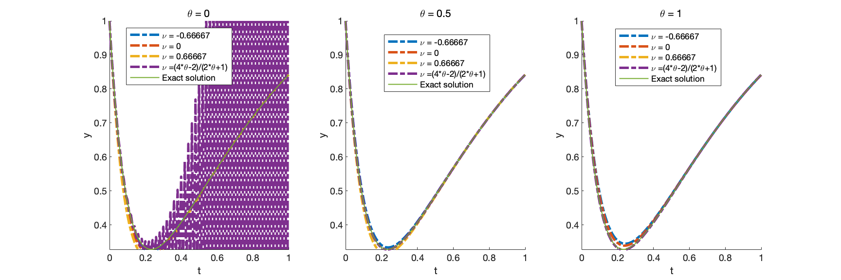
y′=λ​(y−sin⁡t)+cos⁡t,y​(0)=1,0≥t<1,formulae-sequencesuperscript𝑦′𝜆𝑦𝑡𝑡formulae-sequence𝑦010𝑡1y^{\prime}=\lambda(y-\sin{t})+\cos{t},\quad y(0)=1,\quad 0\geq t<1,

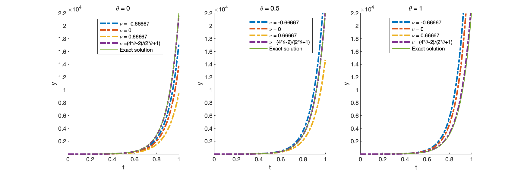
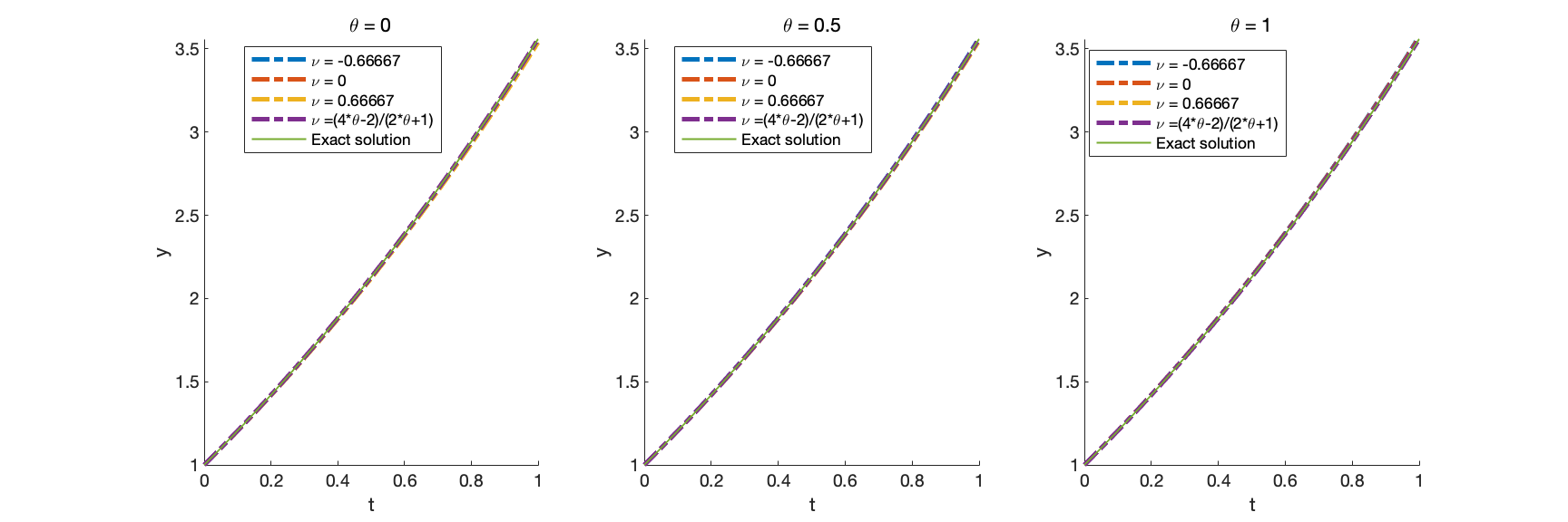
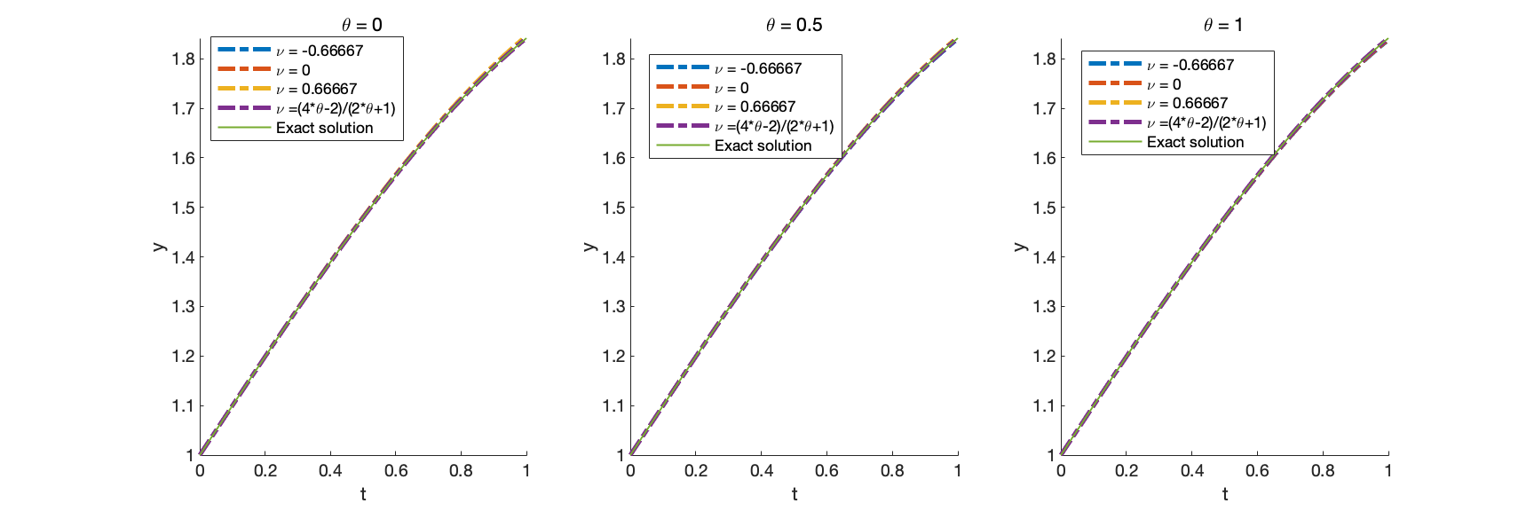
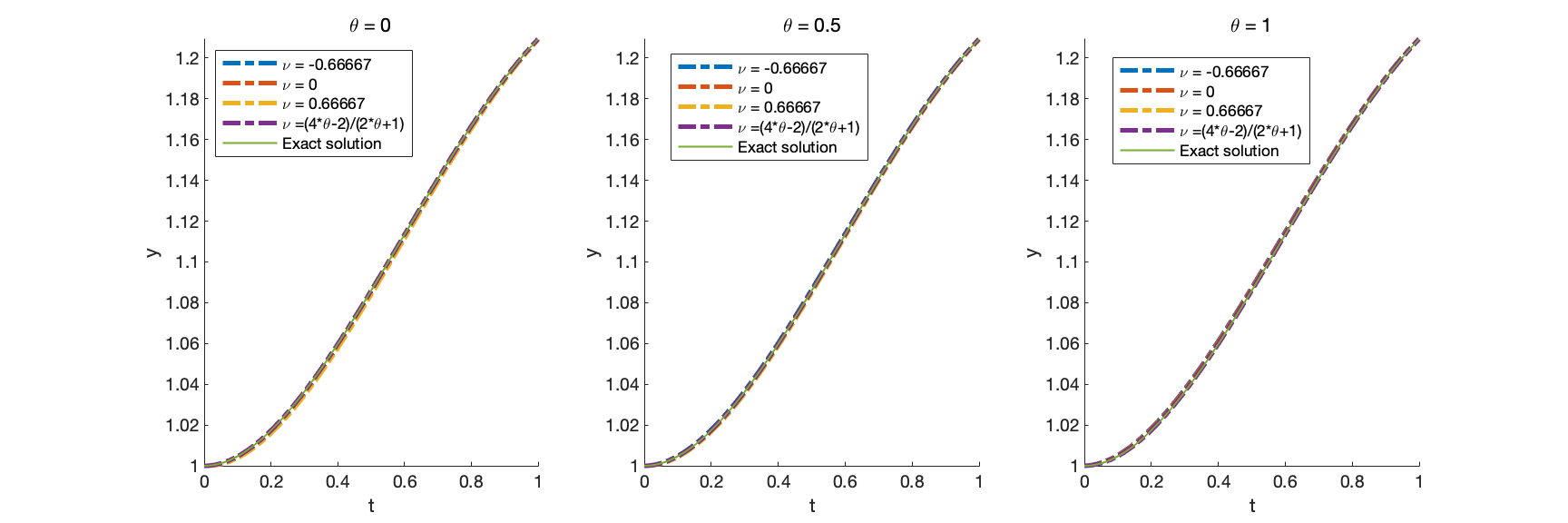
whose exact solution is y​(t)=eλ​t+sin⁡t𝑦𝑡superscript𝑒𝜆𝑡𝑡y(t)=e^{\lambda t}+\sin{t}. Consider using time step k=0.01𝑘0.01k=0.01 for λ=10,1,0,−1,−10,−500𝜆1010110500\lambda=10,1,0,-1,-10,-500.

Remark 14.

In Proposition 3.1, we showed second-order accuracy is attained when ν=(4​θ−2)/(2​θ+1)𝜈4𝜃22𝜃1\nu=(4\theta-2)/(2\theta+1).

  • •

    θ=0𝜃0\theta=0, (4​θ−2)/(2​θ+1)=−24𝜃22𝜃12(4\theta-2)/(2\theta+1)=-2,

  • •

    θ=1/2𝜃12\theta=1/2, (4​θ−2)/(2​θ+1)=04𝜃22𝜃10(4\theta-2)/(2\theta+1)=0,

  • •

    θ=1𝜃1\theta=1, (4​θ−2)/(2​θ+1)=2/34𝜃22𝜃123(4\theta-2)/(2\theta+1)=2/3.

Refer to caption
Fig. 9: λ=10𝜆10\lambda=10
Refer to caption
Fig. 10: λ=1𝜆1\lambda=1
Refer to caption
Fig. 11: λ=0𝜆0\lambda=0
Refer to caption
Fig. 12: λ=−1𝜆1\lambda=-1
Refer to caption
Fig. 13: λ=−10𝜆10\lambda=-10
Refer to caption
Fig. 14: λ=−500𝜆500\lambda=-500

6 Convergence rate

Consider the test problem

y′=λ​(y−sin⁡t)+cos⁡t,y​(0)=1,0≥t<1,formulae-sequencesuperscript𝑦′𝜆𝑦𝑡𝑡formulae-sequence𝑦010𝑡1y^{\prime}=\lambda(y-\sin{t})+\cos{t},\quad y(0)=1,\quad 0\geq t<1,

whose exact solution is y​(t)=eλ​t+sin⁡t𝑦𝑡superscript𝑒𝜆𝑡𝑡y(t)=e^{\lambda t}+\sin{t}. Consider using time step k=0.00125,0.0025,0.005,0.01,0.02𝑘0.001250.00250.0050.010.02k=0.00125,0.0025,0.005,0.01,0.02 for λ=10,1,0,−1,−10𝜆1010110\lambda=10,1,0,-1,-10 to calculate the convergence rate. We got the same result for all cases of λ𝜆\lambda. Hence we showed for the case when λ=−10𝜆10\lambda=-10 in the following tables.

Remark 15.

In Proposition 7, we get second-order accuracy when ν=(4​θ−2)/(2​θ+1)𝜈4𝜃22𝜃1\nu=(4\theta-2)/(2\theta+1).

  • •

    θ=0𝜃0\theta=0, (4​θ−2)/(2​θ+1)=−24𝜃22𝜃12(4\theta-2)/(2\theta+1)=-2,

  • •

    θ=1/2𝜃12\theta=1/2, (4​θ−2)/(2​θ+1)=04𝜃22𝜃10(4\theta-2)/(2\theta+1)=0,

  • •

    θ=1𝜃1\theta=1, (4​θ−2)/(2​θ+1)=2/34𝜃22𝜃123(4\theta-2)/(2\theta+1)=2/3.

Timestep ν=−0.66667𝜈0.66667\nu=-0.66667 Rate ν=0𝜈0\nu=0 Rate ν=0.66667𝜈0.66667\nu=0.66667 Rate ν=4​θ−22​θ+1𝜈4𝜃22𝜃1\nu=\frac{4\theta-2}{2\theta+1} Rate
0.0013 4.9438e-04 - 9.8742e-04 - 0.0020 - 0.1935 -
0.0025 9.9394e-04 1.0075 0.0020 1.0054 0.0040 1.0060 0.7781 2.0074
0.0050 0.0020 1.0158 0.0040 1.0109 0.0080 1.0119 3.1372 2.0115
0.0100 0.0041 1.0348 0.0081 1.0225 0.0163 1.0232 12.6357 2.0100
0.0200 0.0087 1.0849 0.0168 1.0477 0.0335 1.0444 49.4689 1.9690
Table 1: θ=0,λ=−10.formulae-sequence𝜃0𝜆10\theta=0,\ \lambda=-10.
Timestep ν=−0.66667𝜈0.66667\nu=-0.66667 Rate ν=0𝜈0\nu=0 Rate ν=0.66667𝜈0.66667\nu=0.66667 Rate ν=4​θ−22​θ+1𝜈4𝜃22𝜃1\nu=\frac{4\theta-2}{2\theta+1} Rate
0.0013 4.8942e-04 - 2.0649e-06 - 9.8734e-04 - 2.0649e-06 -
0.0025 9.7398e-04 0.9928 8.2597e-06 2.0001 0.0020 1.0052 8.2597e-06 2.0001
0.0050 0.0019 0.9858 3.3044e-05 2.0002 0.0040 1.0103 3.3044e-05 2.0002
0.0100 0.0038 0.9724 1.3226e-04 2.0009 0.0081 1.0200 1.3226e-04 2.0009
0.0200 0.0073 0.9493 5.3042e-04 2.0037 0.0166 1.0377 5.3042e-04 2.0037
Table 2: θ=12,λ=−10.formulae-sequence𝜃12𝜆10\theta=\frac{1}{2},\ \lambda=-10.
Timestep ν=−0.66667𝜈0.66667\nu=-0.66667 Rate ν=0𝜈0\nu=0 Rate ν=0.66667𝜈0.66667\nu=0.66667 Rate ν=4​θ−22​θ+1𝜈4𝜃22𝜃1\nu=\frac{4\theta-2}{2\theta+1} Rate
0.0013 0.0015 - 9.8017e-04 - 1.8416e-05 - 1.8416e-05 -
0.0025 0.0029 0.9945 0.0020 0.9948 7.2888e-05 1.9847 7.2888e-05 1.9847
0.0050 0.0058 0.9892 0.0039 0.9897 2.8546e-04 1.9695 2.8546e-04 1.9695
0.0100 0.0115 0.9786 0.0076 0.9798 0.0011 1.9397 0.0011 1.9397
0.0200 0.0223 0.9581 0.0149 0.9615 0.0040 1.8820 0.0040 1.8820
Table 3: θ=1,λ=−10.formulae-sequence𝜃1𝜆10\theta=1,\ \lambda=-10.

7 Conclusions

Though the result for Backward Euler with time filter is known, we explored all possible choices of θ𝜃\theta in our paper. We have shown that for different choices of ν𝜈\nu, we have different stability regions. We have shown that when θ>1/2𝜃12\theta>1/2, we always have A𝐴A-stability and when θ<1/2𝜃12\theta<1/2, we have A0subscript𝐴0A_{0}-stability or Aπ/4subscript𝐴𝜋4A_{\pi/4}- stability.

Acknowledgement

We want to thank our advisor Professor William J. Layton, for his insightful ideas and guidance throughout the research. We thank NSF for funding the project.

References

  • [1] R. Asselin. Frequency filter for time integrations. Monthly Weather Review, 100(6):487–490, 1972.
  • [2] G. Dahlquist. Some properties of linear multistep and one-leg methods for ordinary diffenretial equations, 1979.
  • [3] A. Guzel and W. Layton. Time filters increase accuracy of the fully implicit method. BIT Numerical Mathematics, 58(2):301–315, 2018.
  • [4] N. Hurl, W. Layton, Y. Li, and C. Trenchea. Stability analysis of the Crank–Nicolson-Leapfrog method with the Robert–Asselin–Williams time filter. BIT Numerical Mathematics, 54(4):1009–1021, 2014.
  • [5] Y. Li and C. Trenchea. Analysis of time filters used with the Leapfrog scheme. In COUPLED VI: proceedings of the VI International Conference on Computational Methods for Coupled Problems in Science and Engineering, pages 1261–1272. CIMNE, 2015.
  • [6] E. N. Lorenz. Deterministic nonperiodic flow. Journal of Atmospheric Sciences, 20(2):130–141, 1963.
  • [7] Y. Qin, Y. Wang, and J. Li. Analysis of a new time filter algorithm for the unsteady Stokes/Darcy model. arXiv preprint arXiv:2204.13881, 2022.
  • [8] P. D. Williams. A proposed modification to the Robert–Asselin time filter. Monthly Weather Review, 137(8):2538–2546, 2009.
  • [9] P. D. Williams. Achieving seventh-order amplitude accuracy in Leapfrog integrations. Monthly Weather Review, 141(9):3037–3051, 2013.