Analyzing Single Cell RNA Sequencing with Topological Nonnegative Matrix Factorization
Abstract
Single-cell RNA sequencing (scRNA-seq) is a relatively new technology that has stimulated enormous interest in statistics, data science, and computational biology due to the high dimensionality, complexity, and large scale associated with scRNA-seq data. Nonnegative matrix factorization (NMF) offers a unique approach due to its meta-gene interpretation of resulting low-dimensional components. However, NMF approaches suffer from the lack of multiscale analysis. This work introduces two persistent Laplacian regularized NMF methods, namely, topological NMF (TNMF) and robust topological NMF (rTNMF). By employing a total of 12 datasets, we demonstrate that the proposed TNMF and rTNMF significantly outperform all other NMF-based methods. We have also utilized TNMF and rTNMF for the visualization of popular Uniform Manifold Approximation and Projection (UMAP) and t-distributed stochastic neighbor embedding (t-SNE).
keywords: Algebraic topology, Persistent Laplacian, scRNA-seq, dimensionality reduction, machine learning
1 Introduction
Single-cell RNA sequencing (scRNA-seq) is a relatively new technology that has unveiled the heterogeneity within cell populations, providing valuable insights into complex biological interactions and pathways, such as cell-cell interactions, differential gene expression, signal transduction pathways, and more [1].
Unlike traditional microarray analysis, often referred to as bulk sequencing, scRNA-seq offers the transcriptomic profile of individual cells. With current technology, it’s possible to sequence more than 20,000 genes and 10,000 samples simultaneously. Standard experimental procedures involve cell isolation, RNA extraction, sequencing, library preparation, and data analysis.
Over the years, numerous data analysis pipelines have been proposed, typically encompassing data preprocessing, batch correction, normalization, dimensionality reduction, feature selection, cell type identification, and downstream analyses to uncover relevant biological functions and pathways [2, 3, 4, 5, 6].
However, scRNA-seq data, in addition to their high dimensionality, are characterized by nonuniform noise, sparsity due to drop-out events and low reading depth, as well as unlabeled data [7]. Consequently, dimensionality reduction and feature selection are essential for successful downstream analysis.
Principal components analysis (PCA), uniform manifold approximation and projection (UMAP), and t-distributed stochastic neighbor embedding (t-SNE) are among the most commonly used dimensionality reduction tools for scRNA-seq data. PCA is often employed as an initial step in analysis pipelines, such as trajectory analysis and data integration [8, 9, 10, 11]. In PCA, the first few components are referred to as the principal components, where the variance of the projected data is maximized. In PCA, each th component is orthogonal to all the components, maximizing the residual data projected onto the th component [12, 13]. Numerous successful extensions to the original formulation have been proposed [14, 15, 16, 17]. However, due to the orthogonality constraint of PCA, the reduced data may contain negative values, making it challenging to interpret.
UMAP and t-SNE are nonlinear dimensionality reduction methods often used for visualization. UMAP constructs a -dimensional weighted graph based on -nearest neighbors and computes the edge-wise cross-entropy between the embedded low-dimensional weighted graph representation, utilizing the fuzzy set cross-entropy loss function [18]. t-SNE computes the pairwise similarity between cells by constructing a conditional probability distribution over pairs of cells. Then, a student t-distribution is used to obtain the probability distribution in the embedded space, and the Kullback-Leibler (KL) divergence between the two probability distributions is minimized to obtain the reduced data [19, 20, 21, 22]. However, due to the stochastic nature of these methods and their instability at dimensions greater than 3 [23], they may not be suitable for downstream analysis.
Nonnegative matrix factorization (NMF) is another dimensionality reduction method in which the objective is to decompose the original count matrix into two nonnegative factor matrices [24, 25]. The resulting basis matrices are often referred to as meta-genes and represent nonnegative linear combinations of the original genes. Consequently, NMF results are highly interpretable. However, the original formulation employs a least-squares optimization scheme, making the method susceptible to outlier errors [26].
To address this issue, Kong et al. [27] introduced robust NMF (rNMF), or -NMF, which utilizes the -norm and can better handle outliers while maintaining comparable computational efficiency to standard NMF. Manifold regularization has also been employed to incorporate geometric structures into dimensionality reduction, utilizing a graph Laplacian, leading to Graph Regularized NMF (GNMF) [28]. Semi-supervised methods, such as those incorporating marker genes [29], similarity and dissimilarity constraints [30], have been proposed to enhance NMF’s robustness. Additionally, various other NMF derivatives have been introduced [31, 32, 33].
Despite these advancements in NMF, manifold regularization remains an essential component to ensure that the lower-dimensional representation of the data can form meaningful clusters. However, using graph Laplacians can only capture a single scale of the data, specifically the scaling factor in the heat kernel. Therefore, single-scale graph Laplacians lack multiscale information.
Eckmann et al. [34] introduced simplicial complexes to the graph Laplacian defined on point cloud data, leading to the combinatorial Laplacian. This can be viewed as a discrete counterpart of the de Rham-Hodge Laplacian on manifolds. Both the Hodge Laplacian and the combinatorial Laplacian are topological Laplacians that give rise to topological invariants in their kernel space, specifically the harmonic spectra. However, the nonharmonic spectra contain algebraic connectivity that cannot be revealed by the topological invariants [35].
A significant development in topological Laplacians occurred in 2019 with the introduction of persistent topological Laplacians. Specifically, evolutionary de Rham theory was introduced to obtain persistent Hodge Laplacians on manifolds [36]. Meanwhile, persistent combinatorial Laplacian [37], also known as the persistent spectral graph or persistent Laplacian (PL), was introduced for point cloud data. These methods have spurred numerous theoretical developments [38, 39, 40, 41, 42] and code construction [43], as well as remarkable applications in various fields, including protein engineering [44], forecasting emerging SARS-CoV-2 variants BA.4/BA.5 [45], and predicting protein-ligand binding affinity [46]. Recently, PL has been shown to improve PCA performance [14, 47].
This growing interest arises from the fact that persistent topological Laplacians represent a new generation of topological data analysis (TDA) methods that address certain limitations of the popular persistent homology [48, 49]. In persistent homology, the goal is to represent data as a topological space, often as simplicial complexes. Then, ideas from algebraic topology, such as connected components, holes, and voids, are used to extract topological invariants during a multiscale filtration. Persistent homology has facilitated topological deep learning (TDL), an emerging field [50]. However, persistent homology is unable to capture the homotopic shape evolution of data. PLs overcome this limitation by tracking changes in non-harmonic spectra, revealing the homotopic shape evolution. Additionally, the persistence of PL’s harmonic spectra recovers all topological invariants from persistent homology.
In this work, we introduce PL-regularized NMF, namely the topological NMF (TNMF) and robust topological NMF (rTNMF). Both TNMF and rTNMF can better capture multiscale geometric information than the standard GNMF and rGNMF. To achieve improved performance, PL is constructed by observing cell-cell interactions at multiple scales through filtration, creating a sequence of simplicial complexes. We can then view the spectra at each complex associated with a filtration to capture both topological and geometric information. Additionally, we introduce -NN based PL to TNMF and rTNMF, referred to as -TNMF and -rTNMF, respectively. The -NN based PL reduces the number of hyperparameters compared to the standard PL algorithm.
The outline of this work is as follows. First, we provide a brief overview of NMF, rNMF, GNMF, and rGNMF. Next, we present a concise theoretical formulation of PL and derive the multiplicative updating scheme for TNMF and rTNMF. Additionally, we introduce an alternative construction of PL, termed -NN PL. Following that, we present a benchmark using 12 publicly available datasets. We have observed that PL can improve NMF performance by up to 0.16 in ARI, 0.08 in NMI, 0.04 in purity, and 0.1 in accuracy.
2 Methods
In this section, we provide a brief overview of NMF methods, namely NMF, rNMF, GNMF, and rGNMF. We then give persistent Laplacian and its construction. Finally, we formulate various PL regularized NMF methods.
2.1 Prior Work
2.1.0.1 NMF
The original formulation of NMF utilizes the Frobenius norm, which assumes that the noise of the data is sample from Gaussian distribution.
| (1) |
where . Lee et al. proposed a multiplicative updating scheme, which preserves the nonnegativity [24]. For the th iteration,
| (2) | |||
| (3) |
Although the updating scheme is simple and effective in many biological data applications, scRNA-seq data is sparse and contains large amount of noise. Therefore, a model that is more robust to noise is necessary for feature selection and dimensionality reduction
2.1.0.2 rNMF
The robust NMF (rNMF) utilizes the norm, which assumes that the noise of the data is sampled from a Laplace distribution, which may be more suitable for a count-based data matrix, like scRNA-seq. The minimization function is given as the following
where . Because -norm utilizes summation over the distance of the original cell feature and the reduced feature, the effect of the outlier will not dominate the loss function as much as the Frobenius norm formulation. RNMF has the following updating scheme
| (4) | |||
| (5) |
where .
2.1.0.3 GNMF amd rGNM
Manifold regularization has been widely utilized in scRNA-seq. Let be a graph, where is the set of vertices, is the set of edges, and is the weight associated with the edges. Here, denotes the -th nearest neighbors of vertex . The heat kernel is often used to construct the weight, and we can construct the adjacency matrix as the following.
| (6) |
Since heat kernel satisfies the conditions as and as , we can construct the graph regularization term, , by looking at the distance .
Here, and are the Laplacian and the degree matrix, given by and , respectively. denotes the trace of the matrix. Utilizing the regularization parameters, , we get the objective function of GNMF
| (7) |
and the objective function for rGNMF
| (8) |
2.2 Topological NMF
While graph regularization improves the traditional NMF and rNMF, the choice of and vastly change the result. Furthermore, graph regularization only captures a single scale, and may not be able to capture the mutliscale geometric information in data. Here, we give a brief introduction to persistent homology and persistent Laplacian and derive the updating scheme for the topological NMF.
2.2.1 Persistent Laplacians
Persistent homology and persistent spectral graphs have been successfully used in biomolecular data [44, 46, 50, 48, 49, 14]. Similar to persistent homology, persistent spectral graphs track birth and death of topological features, i.e., holes, over different scales. However, unlike persistent homology, persistent spectral graphs can further capture the homotopic shape evolution of data during the filtration. Through the filtration process, these methods offer the multiscale analysis of data.
We begin by the definition of simplex. Let denote -simplex, where is a vertex. is a node, is an edge, is a triangle is a tetrahedron, and so on. A simplicial complex is a union of simplicies such that
-
1.
If and is a face of , then
-
2.
The nonempty intersection of any 2 simplicies in is a face of both simplicies.
We can think of as gluing lower dimensional simplicies that satisfies the above 2 properties.
A -chain is a formal sum of -simplicies in with the coefficients . The set of all -chains has contains the basis for the set of -simplicies in . Such set forms a finitely generated free Abelian group . We can relate the chain groups via a boundary operator, which is a group homomorphism . The boundary operator is defined as the following.
| (9) |
where , where is a -simplex with vertex removed. The sequence of chain group connected by the boundary operator defines the chain complex.
| (10) |
The chain complex associated with a simplicial complex defines the -th homology group , and the dimension of is the -dimensional holes, or the th Betti number denoted as . For example, is the number of connected components, is the number of loops and is the number of cavities.
We can now define the dual chain complex through the adjoint operator of . The dual space is defined as , and the coboundary operator is defined as . For and , the coboundary operator is defined as
| (11) |
Here is a cochain, or a homomorphic mapping from a chain to the coefficient group. The homology of the dual chain complex is called the cohomology.
We then define the -combinatorial Laplacian operator
| (12) |
Let be the standard basis for the matrix representation of -boundary operator from and , and be th -coboundary operator. The matrix representation of the -th order Laplacian operator is defined as
| (13) |
The multiplicity of zero eigenvalue of is the -th Betti number of the simplicail complex. The nonzero eigenvalues (non-harmonic spectrum) contains other topological and geometrical features.
As stated before, simplicial complex does not provide sufficient information to understand the geometry of the data. To this end, we utilize simplicial complex induced by filtration
| (14) |
where is the number of filtration.
For each , denote as chain group induced by , and the corresponding boundary operator , resulting in
| (15) |
for . The adjoint operator of is similarity defined as , which we regard as the mapping via the isomorphism between cochain and chain groups. Through these 2 operators, we can define the chain complexes induced by .
Utilizing filtration with simplicial complex, we can define persistence Laplacian spectra. Let whose boundary is in be , assuming an inclusion mapping . On this set, we can define the -persistent -boundary operator denoted and the corresponding adjoint operator . Then, the -order -persistent Laplacian operator is computed as
| (16) |
and its matrix representation as
| (17) |
Likewise as before, the multiplicity of the zero-eigenvalue is the -th order -persistent Betti number , which is the -dimensional hole in that persists in . Moreover, the -th order Laplacian is just a particular case of , where , which is a snapshot of the topology at the filtration step [43, 37].
We can utilize the 0-persistent Laplacian to capture the interactions between the data at different filtration values. In particular, we can perform filtration by computing a family of subgraphs induced by a threshold distance , which is called the Vietoris Rips complex. Alternatively, we can compute a Gaussian Kernel induced distance to construct the subgraphs.
2.2.2 TNMF and rTNMF
For scRNA-seq data, we calculate the 0-persistent Laplacian using the Vietoris-Rips (VR) complexes by increasing the filtration distance. We can then take a weighted sum over the 0-persistent Laplacian induced by the changes in the filtration distance. For persistent Laplacian enhanced NMF, we will provide a computationally efficient algorithm to construct the persistent Laplacian matrix.
Let be a Laplacian matrix induced by some weighted graph, and note the following
Then, let , and . The -th Persistent Laplacian , is defined as , where
| (18) | |||
| (19) |
Then, we can take the weighted sum over the all the persistent Laplacians
| (20) |
Unlike the standard Laplacian matrix , PL captures the topological features that persists over different filtration, thus providing a multiscale view of the data that standard Laplacian lacks. Here, is the hyper-parameter and must be chosen as a hyperparameter. Then, the topological NMF (TNMF) is defined as
| (21) |
and the topological rNMF (rTNMF) is defined as
| (22) |
2.2.3 Multiplicative Updating scheme
The updating scheme follows the same principle as the standard GNMF and rGNMF.
2.2.3.1 TNMF
For top-NMF, the Lagrangian function is defined as
| (23) | ||||
| (24) |
Taking the partial with respect to , we get
| (25) |
Using the KKT condition , we get the following
| (26) |
Therefore, the updating scheme is
| (27) |
For updating , we take the derivative of the Lagrangian function with respect to
| (28) |
Using the Karush–Kuhn–Tucker (KKT) condition, we have and obtain
| (29) |
where and . The updating scheme is then given by
| (30) |
2.2.3.2 rTNMF
For the updating scheme for top-rNMF, we utilize the fact that , where . The Lagrangian is given by
| (31) | ||||
| (32) | ||||
| (33) |
where . Taking the partial with respect to , we get
| (34) |
Using the KKT conditions , we get
| (35) |
which gives the updating scheme
| (36) |
For , we take the partial with respect to .
| (37) |
Then, using the KKT conditions , we get
| (38) |
where and gives the updating scheme
| (39) |
2.3 -NN induced Persistent Laplacian
One major issue with top-GNMF and top-rGNMF is that the parameters have to be chosen. For the parameters, we let for a total of parameters. Therefore, the number of parameters that needs to be chosen increases exponentially as the number of filtration increases. Therefore, we propose an approximation to the original formulation using -NN based persistent Laplacian.
Let be the -nearest neighbors of sample . Then, define the -persistent directed adjacency matrix as
| (40) |
Then, the -NN based directed adjacency Laplacian is the weighted sum of
| (41) |
Then, the undirected persistent adjacency matrix can be obtained via symmetrization
where denote Hadamard product. Then, the persistent Laplacian can be constructed using the persistent degree matrix
| (42) |
One advantage of utilizing the -NN induced persistent Laplacian is that the parameter space is much smaller. We can set , where would ’turn-off’ the particular neighbor’s connectivity. In essence, the number of parameters will be reduced to , a significant decrease from of the original formulation.
2.4 Evaluation metrics
Let and be 2 partitions of the data. Here, we let be the true label partition and be the cluster label partition. Let and be the true and predicted labels of sample .
2.4.0.1 Adjusted Rand Index
Adjusted random index (ARI) measures the similarity between two clustering by observing all pairs of samples that belong to the same cluster, and seeing if the other clustering result also have the same pair of samples in the same cluster [51]. Let be the number of samples that belong to true label and cluster label , and define and . Then, the ARI is defined as
| (43) |
The ARI takes on a value between -1 and 1, where 1 is a perfect match between two clustering methods, and 0 is a completely random assignment of labels, and -1 indicates that the two clusterings are completely different.
2.4.0.2 Normalized Mutual Information
The normalized mutual information (NMI) measures the mutual information between two clustering results and normalized according to cluster size [52]. We fix the true labels as one of the clustering result, and use the predicted labels as the other to calculate NMI. The NMI is calculated as the following
| (44) |
where is the entropy and is the mutual information between true labels and predicted labels . NMI has a range of 0 and 1, where 1 is a perfect mutual correlation between the two sets of labels and 0 means no mutual information.
2.4.0.3 Accuracy
Accuracy (ACC) calculates the percentage of correctly predicted class labels. The accuracy is given by
| (45) |
where is the indicator function, where if , , and 0 otherwise. maps the cluster labels to the true labels, where the mapping is the optimal permutation of the cluster labels and true labels obtained from the Hungarian algorithm [53].
2.4.0.4 Purity
For purity calculation, each predicted label is assigned to a true label such that the is maximized [54]. Taking the average over all the predicted label, we obtain the following
| (46) |
Note that unlike accuracy, purity does not map the predicted labels to the true labels.
3 Results
3.1 Benchmark Data
We have performed benchmark on 12 publicly available datasets. The GEO accession number, reference, organism, number of cell types, and number of samples are recorded in Table 1. For each data, cell types with less than 15 cells were removed. Log-normalization was applied, and scaled the data to have unit length. For GNMF and rGNMF, neighbors were used. For TNMF and rTNMF, 8 filtration values were used to construct PL, and for each scale, binary selection was used. for -TNMF and -rTNMF, was used with . For each test, double nonnegative singular value decomposition with zeros filled with the average of (NNDSVDA) was used for the initialization. The -means clustering was applied to obtain the clustering results.
| Geo Accession | Reference | Organism | Cell type | Number of Samples | Number of Genes |
|---|---|---|---|---|---|
| GSE67835 | Dramanis [55] | Human | 8 | 420 | 22084 |
| GSE75748 time | Chu [56] | Human | 6 | 758 | 19189 |
| GSE82187 | Gokce [57] | Mouse | 8 | 705 | 18840 |
| GSE84133human1 | Baron [58] | Human | 9 | 1895 | 20125 |
| GSE84133human2 | Baron [58] | Human | 9 | 1702 | 20125 |
| GSE84133human3 | Baron [58] | Human | 9 | 3579 | 20125 |
| GSE84133human4 | Baron [58] | Human | 6 | 1275 | 20125 |
| GSE84133mouse1 | Baron [58] | Mouse | 6 | 782 | 14878 |
| GSE84133mouse2 | Baron [58] | Mouse | 8 | 1036 | 14878 |
| GSE57249 | Biase [59] | Human | 3 | 49 | 25737 |
| GSE64016 | Leng [60] | Human | 4 | 460 | 19084 |
| GSE94820 | Villani [61] | Human | 5 | 1140 | 26593 |
3.2 Benchmarking PL regularized NMF
In order to benchmark persistent Laplacain regularized NMF, we compared our methods to other commonly used NMF methods, namely the GNMF, rGNMF, rNMF and NMF. For a fair comparison, We omitted supervised or semi-supervised methods. For -rTNMF, rTNMF, -TNMF, TNMF, GNMF and rGNMF, we set for all tests.
Table 2 shows the ARI values of the NMF methods for the 12 data we have tested. The bold number indicate the highest performance. Figure 1 depicts the average ARI value over the 12 datasets for each method.
| data | -rTNMF | rTNMF | -TNMF | TNMF | rGNMF | GNMF | rNMF | NMF |
|---|---|---|---|---|---|---|---|---|
| GSE67835 | 0.9454 | 0.9236 | 0.9306 | 0.8533 | 0.9391 | 0.9109 | 0.7295 | 0.7314 |
| GSE64016 | 0.2569 | 0.1544 | 0.2237 | 0.1491 | 0.1456 | 0.1605 | 0.1455 | 0.1466 |
| GSE75748time | 0.6421 | 0.6581 | 0.5963 | 0.6099 | 0.6104 | 0.5790 | 0.5969 | 0.5996 |
| GSE82187 | 0.9877 | 0.9815 | 0.9676 | 0.9809 | 0.7558 | 0.7577 | 0.8221 | 0.8208 |
| GSE84133human1 | 0.8310 | 0.8969 | 0.8301 | 0.8855 | 0.8220 | 0.7907 | 0.7080 | 0.6120 |
| GSE84133human2 | 0.9469 | 0.9072 | 0.9433 | 0.9255 | 0.9350 | 0.9255 | 0.8930 | 0.8929 |
| GSE84133human3 | 0.8504 | 0.9179 | 0.8625 | 0.9181 | 0.8447 | 0.8361 | 0.7909 | 0.8089 |
| GSE84133human4 | 0.8712 | 0.9692 | 0.8712 | 0.9692 | 0.8699 | 0.8681 | 0.8311 | 0.8311 |
| GSE84133mouse1 | 0.8003 | 0.7894 | 0.8003 | 0.7913 | 0.7945 | 0.7918 | 0.6428 | 0.6348 |
| GSE84133mouse2 | 0.6953 | 0.8689 | 0.7005 | 0.9331 | 0.6808 | 0.6957 | 0.5436 | 0.5470 |
| GSE57249 | 1.0000 | 0.9638 | 1.0000 | 0.9483 | 1.0000 | 1.0000 | 0.9483 | 0.9483 |
| GSE94820 | 0.6101 | 0.5480 | 0.4916 | 0.5574 | 0.5139 | 0.5189 | 0.5440 | 0.5556 |

Overall, PL regularized rNMF and NMF have the highest ARI value across all the datasets. -rTNMF outperforms other NMF methods by at least 0.09 for GSE64016. All PL regularized NMF methods outperform other NMF methods by at least 0.14 for GSE82187. For GSE84133 human 3, both rTNMF and TNMF outperform other methods by 0.07. TNMF improves other methods by more than 0.2 for GSE84133 mouse 2. Lastly, -rTNMF has the highest ARI value for GSE94820. Moreover, rTNMF improves rGNMF by 0.05, and TNMF improves GNMF by about 0.06. -TNMF and -rTNMF also improve GNMF and rGNMF by about 0.03.
Table 3 shows the NMI values of of the NMF methods for the 12 datasets we have tested. The bold number indicate the highest performance. Figure 2 shows the average NMI value over the 12 datasets.
| data | -rTNMF | rTNMF | -TNMF | TNMF | rGNMF | GNMF | rNMF | NMF |
|---|---|---|---|---|---|---|---|---|
| GSE67835 | 0.9235 | 0.8999 | 0.9107 | 0.8607 | 0.9104 | 0.8858 | 0.7975 | 0.8017 |
| GSE64016 | 0.3057 | 0.2059 | 0.3136 | 0.1869 | 0.2593 | 0.2562 | 0.1896 | 0.1849 |
| GSE75748time | 0.7522 | 0.7750 | 0.7159 | 0.7343 | 0.7235 | 0.6971 | 0.7227 | 0.7244 |
| GSE82187 | 0.9759 | 0.9691 | 0.9298 | 0.9668 | 0.8802 | 0.8754 | 0.9124 | 0.9117 |
| GSE84133human1 | 0.8802 | 0.8716 | 0.8785 | 0.8780 | 0.8713 | 0.8310 | 0.8226 | 0.7949 |
| GSE84133human2 | 0.9363 | 0.8937 | 0.9313 | 0.9070 | 0.9237 | 0.9145 | 0.8835 | 0.8829 |
| GSE84133human3 | 0.8500 | 0.8718 | 0.8577 | 0.8677 | 0.8439 | 0.8357 | 0.8215 | 0.8260 |
| GSE84133human4 | 0.8795 | 0.9542 | 0.8795 | 0.9542 | 0.8775 | 0.8753 | 0.8694 | 0.8694 |
| GSE84133mouse1 | 0.8664 | 0.8498 | 0.8664 | 0.8495 | 0.8596 | 0.8565 | 0.7634 | 0.7593 |
| GSE84133mouse2 | 0.8218 | 0.8355 | 0.8299 | 0.8713 | 0.8005 | 0.8129 | 0.7258 | 0.7272 |
| GSE57249 | 1.0000 | 0.9505 | 1.0000 | 0.9293 | 1.0000 | 1.0000 | 0.9293 | 0.9293 |
| GSE94820 | 0.7085 | 0.6657 | 0.6157 | 0.6716 | 0.6195 | 0.6258 | 0.6624 | 0.6693 |

Interestingly, -rTNMF and -TNMF on average have higher NMI values than rTNMF and TNMF, respectively. However, all PL regularized methods outperform rGNMF, GNMF, rNMF and NMF. Overall, PL regularized methods outperform other methods. Most noticeably, -rTNMF, rTNMF and TNMF outperform standard NMF methods by 0.06 for GSE82187. Both rTNMF and TNMf outperform rGNMF and GNMF by 0.08 for GSE84133 human 4.
Table 4 shows the purity values of the NMF methods for the 12 datasets we have tested. The bold number indicate the highest performance. Figure 3 shows the average purity over the 12 datasets.
| data | -rTNMF | rTNMF | -TNMF | TNMF | rGNMF | GNMF | rNMF | NMF |
|---|---|---|---|---|---|---|---|---|
| GSE67835 | 0.9643 | 0.9267 | 0.9595 | 0.9024 | 0.9595 | 0.9476 | 0.8726 | 0.8719 |
| GSE64016 | 0.6048 | 0.4913 | 0.5846 | 0.5013 | 0.5339 | 0.5398 | 0.5080 | 0.5050 |
| GSE75748time | 0.7736 | 0.7512 | 0.7533 | 0.7454 | 0.7553 | 0.7387 | 0.7467 | 0.7455 |
| GSE82187 | 0.9927 | 0.9895 | 0.9620 | 0.9888 | 0.9620 | 0.9594 | 0.9693 | 0.9692 |
| GSE84133human1 | 0.9543 | 0.9357 | 0.9536 | 0.9382 | 0.9490 | 0.9187 | 0.9189 | 0.9099 |
| GSE84133human2 | 0.9818 | 0.9614 | 0.9806 | 0.9661 | 0.9777 | 0.9736 | 0.9602 | 0.9600 |
| GSE84133human3 | 0.9472 | 0.9485 | 0.9531 | 0.9460 | 0.9452 | 0.9420 | 0.9464 | 0.9466 |
| GSE84133human4 | 0.9427 | 0.9882 | 0.9427 | 0.9882 | 0.9427 | 0.9420 | 0.9412 | 0.9412 |
| GSE84133mouse1 | 0.9565 | 0.9540 | 0.9565 | 0.9540 | 0.9552 | 0.9540 | 0.9309 | 0.9299 |
| GSE84133mouse2 | 0.9585 | 0.9410 | 0.9604 | 0.9373 | 0.9466 | 0.9507 | 0.9185 | 0.9199 |
| GSE57249 | 1.0000 | 0.9857 | 1.0000 | 0.9796 | 1.0000 | 1.0000 | 0.9796 | 0.9796 |
| GSE94820 | 0.7893 | 0.7462 | 0.6658 | 0.7550 | 0.6421 | 0.6421 | 0.7429 | 0.7531 |

In general, PL-regularized methods achieve higher purity values compared to other NMF methods. Purity measures the maximum intersection between true and predicted classes, which is why we do not observe a significant difference, as seen in ARI and NMI. Furthermore, since purity does not account for the size of a class, and given the imbalanced class sizes in scNRA-seq data, it is not surprising that the purity values are similar.
Table 5 shows the ACC of the NMF methods for the 12 datasets we have tested. The bold number indicate the highest performance. Figure 4 shows the average ACC over the 12 datasets.
| data | -rTNMF | rTNMF | -TNMF | TNMF | rGNMF | GNMF | rNMF | NMF |
|---|---|---|---|---|---|---|---|---|
| GSE67835 | 0.9643 | 0.9243 | 0.9595 | 0.9000 | 0.9595 | 0.9383 | 0.8357 | 0.8364 |
| GSE64016 | 0.5700 | 0.4870 | 0.5502 | 0.4746 | 0.4891 | 0.4537 | 0.4691 | 0.4759 |
| GSE75748time | 0.7565 | 0.7438 | 0.7414 | 0.6917 | 0.7355 | 0.7241 | 0.6873 | 0.6875 |
| GSE82187 | 0.9927 | 0.9895 | 0.9599 | 0.9888 | 0.8512 | 0.8514 | 0.8896 | 0.8889 |
| GSE84133human1 | 0.8973 | 0.9194 | 0.8974 | 0.9088 | 0.8889 | 0.8364 | 0.7988 | 0.7370 |
| GSE84133human2 | 0.9260 | 0.9069 | 0.9242 | 0.9447 | 0.9224 | 0.9177 | 0.8998 | 0.8994 |
| GSE84133human3 | 0.8539 | 0.9456 | 0.8597 | 0.9419 | 0.8498 | 0.8228 | 0.8032 | 0.8178 |
| GSE84133human4 | 0.8831 | 0.9882 | 0.8831 | 0.9882 | 0.8824 | 0.8816 | 0.8847 | 0.8847 |
| GSE84133mouse1 | 0.8581 | 0.8542 | 0.8581 | 0.8542 | 0.8555 | 0.8542 | 0.7361 | 0.7311 |
| GSE84133mouse2 | 0.8232 | 0.9101 | 0.8263 | 0.9305 | 0.7903 | 0.8155 | 0.7239 | 0.7294 |
| GSE57249 | 1.0000 | 0.9857 | 1.0000 | 0.9796 | 1.0000 | 1.0000 | 0.9796 | 0.9796 |
| GSE94820 | 0.7533 | 0.7119 | 0.6482 | 0.7201 | 0.6088 | 0.6107 | 0.7091 | 0.7189 |

Once again, we see that PL regularized methods have higher ACC than other NMF methods. RTNMF and TNMF improves rGNMF and GNMF by 0.05, and -rTNMF and -TNMF improves rGNMF and GNMF by 0.04. We see an improvement in ACC for both -rTNMF and -TNMF for GSE64016. All 4 PL regularized methods improve ACC of GSE82187 by 0.1. RTNMF and TNMF improve GSE84133 mouse 2 by at least 0.1 as well.
3.3 Overall performance
Figure 5 shows the average ARI, NMI, purity and ACC of -rTNMF, rTNMF, -TNMF, TNMF, rGNMF, GNMF, rNMF, NMF across 10 datasets. All PL regularized NMF methods outperform the traditional rGNMF, GNMF, rNMF and NMF. Both rTNMF and TNMF have higher average ARI and purity than the -NN based PL counterparts. However, -rTNMF and -TNMF have higher average NMI than rTNMF and TNMF, respectively. -rTNMF has a significantly higher purity than other methods.

4 Discussion
4.1 Visualization of meta-genes based UMAP and t-SNE
Both UMAP and t-SNE are well-known for their effectiveness in visualization. However, these methods may not perform as competitively in clustering or classification tasks. Therefore, it is beneficial to employ NMF-based methods to enhance the visualization capabilities of UMAP and t-SNE.
In this process, we generate meta-genes and subsequently utilize UMAP or t-SNE to further reduce the data to 2 dimensions for visualization. For a dataset with cells, the number of meta-genes will be the integer value of . To compare the standard UMAP and t-SNE plots with the top-NMF-assisted and top-rNMF-assisted UMAP and t-SNE visualizations, we used the default settings of the Python implementation of UMAP and the Scikit-learn implementation of t-SNE. For unassisted UMAP and t-SNE, we first removed low-abundance genes and performed log-transformation before applying UMAP and t-SNE.
Figure 6 shows the visualization of PL regularized NMF methods through UMAP. Each row corresponds to GSE67835, GSE75748 time, GSE94820 and GSE84133 mouse 2 data. The columns from left to right are the -rTNMF assisted UMAP, rTNMF assisted UMAP, -TNMF assisted UMAP, TNMF assisted UMAP and UMAP visualization. Samples were colored according to their true cell types.

Figure 7 shows the visualization of PL regularized NMF through t-SNE. Each row corresponds to GSE67835, GSE75748 time, GSE94820 and GSE84133 mouse 2 data. The columns from left to right are the -rTNMF assisted t-SNE, rTNMF assisted t-SNE, -TNMF assisted t-SNE, TNMF assisted t-SNE and t-SNE visualization. Samples were colored according to their true cell types.

We see a considerable improvement in both top-NMF assisted and top-rNMF assisted UMAP and t-SNE visualization.
4.1.0.1 GSE67835
In the assisted UMAP and t-SNE visualizations of GSE67835, we observe a more distinct cluster, which includes a supercluster of fetal quiescent (Fetal-Q) and fetal replicating (Fetal-R) cells. Darmanis et al. [55] conducted a study that involved obtaining differential gene expression data for human adult brain cells and sequencing fetal brain cells for comparison. It is not surprising that the undeveloped Fetal-Q and Fetal-R cells do not exhibit significant differences and cluster together.
4.1.0.2 GSE75748 time
In GSE75748 time data, Chu et al. [56] sequenced human embryonic stem cells at times 0hr, 12hr, 24hr, 36hr, 72hr, and 96hr under hypoxic conditions to observe differentiation. In unassisted UMAP and t-SNE, although some clustering is visible, there is no clear separation between the clusters. Additionally, two subclusters of 12hr cells are observed.
Notably, in the PL-regularized assisted UMAP and t-SNE visualizations, there is a distinct supercluster comprising the 72hr and 96hr cells, while cells from different time points form their own separate clusters. This finding aligns with Chu’s observation that there was no significant difference between the 72hr and 96hr cells, suggesting that differentiation may have already occurred by the 72hr mark.
4.1.0.3 GSE94820
Notice that in both t-SNE and UMAP, although there is a boundary, the cells do not form distinct clusters. This lack of distinct clustering can pose challenges in many clustering and classification methods. On the other hand, all PL-regularized NMF methods result in distinct clusters.
Among the PL-regularized NMF approaches, cutoff-based PL, rTNMF, and TNMF form a single CD1C+ (CD1C1) cluster, whereas the -NN induced PL, -rTNMF, and -TNMF exhibit two subclusters. Villani et al. [61] previously noted the similarity in the expression profile of CD1C1-CD141- (DoubleNeg) cells and monocytes. PL-regularized NMF successfully differentiates between these two types.
4.1.0.4 GSE84133 mouse 2
PL-regularized NMF yields significantly more distinct clusters compared to unassisted UMAP and t-SNE. Notably, the beta and gamma cells form distinct clusters in PL-regularized NMF. Additionally, when PL-regularized NMF is applied to assist UMAP, potential outliers within the beta cell population become visible. Baron et al. [58] previously highlighted heterogeneity within the beta cell population, and we observe potential outliers in all visualizations.
4.2 RS analysis
Although UMAP and t-SNE are excellent tools for visualizing clusters, they may struggle to capture heterogeneity within clusters. Moreover, these methods can be less effective when dealing with a large number of classes. Therefore, it is essential to explore alternative visualization techniques.
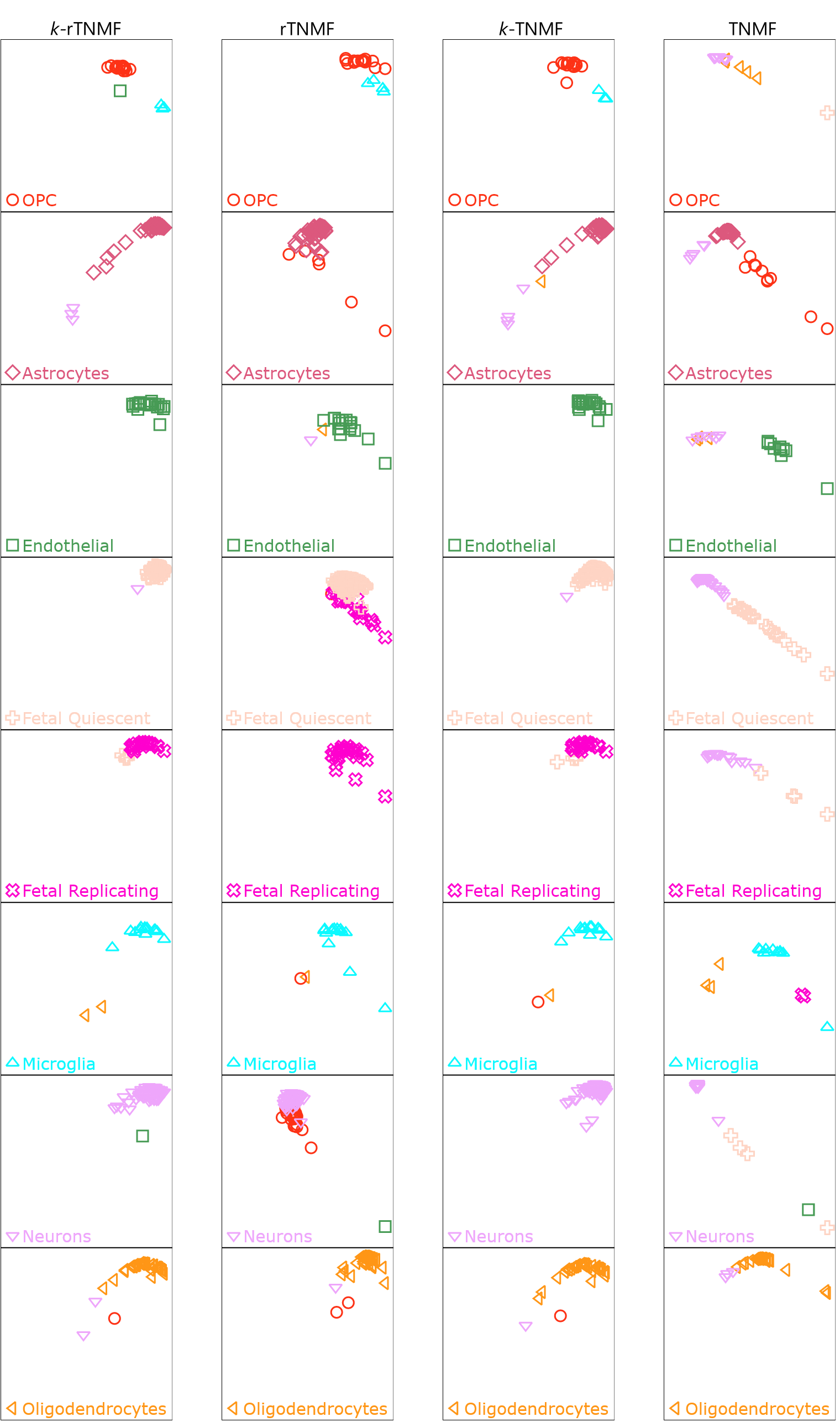
In our approach, we visualize each cluster using RS plots [23]. RS plots depict the relationship between the residue score (R score) and similarity score (S score) and have proven useful in various applications for visualizing data with multiple class types [62, 63, 64, 65, 14].
Let be the data, where is the th sample, is the cell type or cluster label. is the number of class. That is, and .
The residue (R) score is defined as the inter-class sum of distance. For a given data with assignment , the R-score is defined as
where . The similarity (S) score is defined as the intra-class average of distance, defined as
where and is the number of data in class . Both and are bounded by 0 and 1, and the larger the better for a given dataset.
The class residue index (CRI) and the class similarity index (CSI) can then be defined as the average of the R-score and S-score of each of the classes. That is and . Then, the residue index (RI) and the similarity index (SI) can be defined and , respectively.
Using the RI and SI, the residue similarity disparity can be computed by taking , and the residue-similarity index (RSI) can be computed as .
Figure 8 shows the RS plots of PL-regularized NMF methods for GSE67835 data. The columns from left to right correspond to -rTNMF, rTNMF, -TNMF, and TNMF, while the rows correspond to the cell types. The x-axis and y-axis represent the S-score and R-score for each sample, respectively. The samples are colored according to their predicted cell types. Predictions were obtained using k-means clustering, and the Hungarian algorithm was employed to find the optimal mapping from the cluster labels to the true cell types.
We can see that TNMF fails to identify OP cells, whereas -rTNMF, rTNMF, and -TNMF are able to identify OPC cells. Notably, the S-score is quite low, indicating that the OPC did not form a cluster for TNMF. For fetal quiescent and replicating cells, -rTNMF correctly identifies these two types, and the few misclassified samples are located on the boundaries. RTNMF is able to correctly identify fetal replicating cells but could not distinguish fetal quiescent cells from fetal replicating cells. The S-score is low for neurons in both rTNMF and TNMF, which shows a direct correlation with the number of misclassified cells.
5 Conclusion
Persistent Laplacian-regularized NMF is a dimensionality reduction technique that incorporates multiscale topological interactions between the cells. Traditional graph Laplacian-based regularization only represents a single scale and cannot capture the multiscale features of the data. We have also shown that the -NN induced persistent Laplacian outperforms other NMF methods and is comparable to the cutoff-based persistent Laplacian-regularized NMF methods. However, PL methods do come with their downside. In particular, the weights for each filtration must be determined prior to the reduction. If there are filtrations, then the hyperparameter space is . However, -NN induced PL reduces the number of parameters to . In addition, we have shown that we can achieve a significant improvement even if we limit the hyperparameter space to . We would like to further explore possible parameter-free versions of topological NMF. Additionally, NMF methods are not globally convex, but we have shown that with NNDSVDA initialization, our methods perform the best. One possible extension to the proposed methods is to incorporate higher-order persistent Laplacians in the regularization framework, which will reveal higher-order interactions. In addition, we would like to expand the ideas to tensor decomposition, such as Canonical Polyadic Decomposition (CPD) and Tucker decomposition, multimodal omics data, and spatial transcriptomics data.
6 Data availability and code
The data and model used to produce these results can be obtained at https://github.com/hozumiyu/TopologicalNMF-scRNAseq.
7 Acknowledgment
This work was supported in part by NIH grants R01GM126189, R01AI164266, and R35GM148196, National Science Foundation grants DMS2052983, DMS-1761320, and IIS-1900473, NASA grant 80NSSC21M0023, Michigan State University Research Foundation, and Bristol-Myers Squibb 65109.
References
- [1] Aaron TL Lun, Davis J McCarthy, and John C Marioni. A step-by-step workflow for low-level analysis of single-cell rna-seq data with bioconductor. F1000Research, 2016.
- [2] Byungjin Hwang, Ji Hyun Lee, and Duhee Bang. Single-cell rna sequencing technologies and bioinformatics pipelines. Experimental & molecular medicine, 50(8):1–14, 2018.
- [3] Tallulah S Andrews, Vladimir Yu Kiselev, Davis McCarthy, and Martin Hemberg. Tutorial: guidelines for the computational analysis of single-cell rna sequencing data. Nature protocols, 16(1):1–9, 2021.
- [4] Malte D Luecken and Fabian J Theis. Current best practices in single-cell rna-seq analysis: a tutorial. Molecular systems biology, 15(6):e8746, 2019.
- [5] Geng Chen, Baitang Ning, and Tieliu Shi. Single-cell rna-seq technologies and related computational data analysis. Frontiers in genetics, page 317, 2019.
- [6] Raphael Petegrosso, Zhuliu Li, and Rui Kuang. Machine learning and statistical methods for clustering single-cell rna-sequencing data. Briefings in bioinformatics, 21(4):1209–1223, 2020.
- [7] David Lähnemann, Johannes Köster, Ewa Szczurek, Davis J McCarthy, Stephanie C Hicks, Mark D Robinson, Catalina A Vallejos, Kieran R Campbell, Niko Beerenwinkel, Ahmed Mahfouz, et al. Eleven grand challenges in single-cell data science. Genome biology, 21(1):1–35, 2020.
- [8] Gioele La Manno, Ruslan Soldatov, Amit Zeisel, Emelie Braun, Hannah Hochgerner, Viktor Petukhov, Katja Lidschreiber, Maria E Kastriti, Peter Lönnerberg, Alessandro Furlan, et al. Rna velocity of single cells. Nature, 560(7719):494–498, 2018.
- [9] Volker Bergen, Marius Lange, Stefan Peidli, F Alexander Wolf, and Fabian J Theis. Generalizing rna velocity to transient cell states through dynamical modeling. Nature biotechnology, 38(12):1408–1414, 2020.
- [10] Malte D Luecken, Maren Büttner, Kridsadakorn Chaichoompu, Anna Danese, Marta Interlandi, Michaela F Müller, Daniel C Strobl, Luke Zappia, Martin Dugas, Maria Colomé-Tatché, et al. Benchmarking atlas-level data integration in single-cell genomics. Nature methods, 19(1):41–50, 2022.
- [11] Tim Stuart, Andrew Butler, Paul Hoffman, Christoph Hafemeister, Efthymia Papalexi, William M Mauck, Yuhan Hao, Marlon Stoeckius, Peter Smibert, and Rahul Satija. Comprehensive integration of single-cell data. Cell, 177(7):1888–1902, 2019.
- [12] George H Dunteman. Principal components analysis, volume 69. Sage, 1989.
- [13] Ian T Jolliffe and Jorge Cadima. Principal component analysis: a review and recent developments. Philosophical transactions of the royal society A: Mathematical, Physical and Engineering Sciences, 374(2065):20150202, 2016.
- [14] Sean Cottrell, Rui Wang, and Guowei Wei. PLPCA: Persistent Laplacian enhanced-PCA for microarray data analysis. Journal of Chemical Information and Modeling, doi.org/10.1021/acs.jcim.3c01023, 2023.
- [15] Karim Lounici. Sparse principal component analysis with missing observations. In High Dimensional Probability VI: The Banff Volume, pages 327–356. Springer, 2013.
- [16] Hui Zou, Trevor Hastie, and Robert Tibshirani. Sparse principal component analysis. Journal of computational and graphical statistics, 15(2):265–286, 2006.
- [17] F William Townes, Stephanie C Hicks, Martin J Aryee, and Rafael A Irizarry. Feature selection and dimension reduction for single-cell rna-seq based on a multinomial model. Genome biology, 20:1–16, 2019.
- [18] Leland McInnes, John Healy, and James Melville. Umap: Uniform manifold approximation and projection for dimension reduction. arXiv preprint arXiv:1802.03426, 2018.
- [19] Geoffrey E Hinton and Sam Roweis. Stochastic neighbor embedding. Advances in neural information processing systems, 15, 2002.
- [20] Laurens Van der Maaten and Geoffrey Hinton. Visualizing data using t-sne. Journal of machine learning research, 9(11), 2008.
- [21] Dmitry Kobak and George C Linderman. Initialization is critical for preserving global data structure in both t-sne and umap. Nature biotechnology, 39(2):156–157, 2021.
- [22] Etienne Becht, Leland McInnes, John Healy, Charles-Antoine Dutertre, Immanuel WH Kwok, Lai Guan Ng, Florent Ginhoux, and Evan W Newell. Dimensionality reduction for visualizing single-cell data using umap. Nature biotechnology, 37(1):38–44, 2019.
- [23] Yuta Hozumi, Rui Wang, and Guo-Wei Wei. Ccp: correlated clustering and projection for dimensionality reduction. arXiv preprint arXiv:2206.04189, 2022.
- [24] Daniel Lee and H Sebastian Seung. Algorithms for non-negative matrix factorization. Advances in neural information processing systems, 13, 2000.
- [25] Yu-Xiong Wang and Yu-Jin Zhang. Nonnegative matrix factorization: A comprehensive review. IEEE Transactions on knowledge and data engineering, 25(6):1336–1353, 2012.
- [26] Weixiang Liu, Nanning Zheng, and Qubo You. Nonnegative matrix factorization and its applications in pattern recognition. Chinese Science Bulletin, 51:7–18, 2006.
- [27] Deguang Kong, Chris Ding, and Heng Huang. Robust nonnegative matrix factorization using l21-norm. In Proceedings of the 20th ACM international conference on Information and knowledge management, pages 673–682, 2011.
- [28] Qiu Xiao, Jiawei Luo, Cheng Liang, Jie Cai, and Pingjian Ding. A graph regularized non-negative matrix factorization method for identifying microrna-disease associations. Bioinformatics, 34(2):239–248, 2018.
- [29] Peng Wu, Mo An, Hai-Ren Zou, Cai-Ying Zhong, Wei Wang, and Chang-Peng Wu. A robust semi-supervised nmf model for single cell rna-seq data. PeerJ, 8:e10091, 2020.
- [30] Zhenqiu Shu, Qinghan Long, Luping Zhang, Zhengtao Yu, and Xiao-Jun Wu. Robust graph regularized nmf with dissimilarity and similarity constraints for scrna-seq data clustering. Journal of Chemical Information and Modeling, 62(23):6271–6286, 2022.
- [31] Wei Lan, Jianwei Chen, Qingfeng Chen, Jin Liu, Jianxin Wang, and Yi-Ping Phoebe Chen. Detecting cell type from single cell rna sequencing based on deep bi-stochastic graph regularized matrix factorization. bioRxiv, pages 2022–05, 2022.
- [32] Jin-Xing Liu, Dong Wang, Ying-Lian Gao, Chun-Hou Zheng, Jun-Liang Shang, Feng Liu, and Yong Xu. A joint-l2, 1-norm-constraint-based semi-supervised feature extraction for rna-seq data analysis. Neurocomputing, 228:263–269, 2017.
- [33] Na Yu, Ying-Lian Gao, Jin-Xing Liu, Juan Wang, and Junliang Shang. Robust hypergraph regularized non-negative matrix factorization for sample clustering and feature selection in multi-view gene expression data. Human genomics, 13(1):1–10, 2019.
- [34] Beno Eckmann. Harmonische funktionen und randwertaufgaben in einem komplex. Commentarii Mathematici Helvetici, 17(1):240–255, 1944.
- [35] Danijela Horak and Jürgen Jost. Spectra of combinatorial laplace operators on simplicial complexes. Advances in Mathematics, 244:303–336, 2013.
- [36] Jiahui Chen, Rundong Zhao, Yiying Tong, and Guo-Wei Wei. Evolutionary de rham-hodge method. Discrete and continuous dynamical systems. Series B, 26(7):3785, 2021.
- [37] Rui Wang, Duc Duy Nguyen, and Guo-Wei Wei. Persistent spectral graph. International journal for numerical methods in biomedical engineering, 36(9):e3376, 2020.
- [38] Facundo Mémoli, Zhengchao Wan, and Yusu Wang. Persistent laplacians: Properties, algorithms and implications. SIAM Journal on Mathematics of Data Science, 4(2):858–884, 2022.
- [39] Jian Liu, Jingyan Li, and Jie Wu. The algebraic stability for persistent laplacians. arXiv preprint arXiv:2302.03902, 2023.
- [40] Xiaoqi Wei and Guo-Wei Wei. Persistent sheaf laplacians. arXiv preprint arXiv:2112.10906, 2021.
- [41] Rui Wang and Guo-Wei Wei. Persistent path laplacian. Foundations of Data Science, 5:26–55, 2023.
- [42] Dong Chen, Jian Liu, Jie Wu, and Guo-Wei Wei. Persistent hyperdigraph homology and persistent hyperdigraph laplacians. Foundations of Data Science, doi: 10.3934/fods.2023010, 2023.
- [43] Rui Wang, Rundong Zhao, Emily Ribando-Gros, Jiahui Chen, Yiying Tong, and Guo-Wei Wei. Hermes: Persistent spectral graph software. Foundations of data science (Springfield, Mo.), 3(1):67, 2021.
- [44] Yuchi Qiu and Guo-Wei Wei. Persistent spectral theory-guided protein engineering. Nature Computational Science, 3(2):149–163, 2023.
- [45] Jiahui Chen, Yuchi Qiu, Rui Wang, and Guo-Wei Wei. Persistent laplacian projected omicron ba. 4 and ba. 5 to become new dominating variants. Computers in Biology and Medicine, 151:106262, 2022.
- [46] Zhenyu Meng and Kelin Xia. Persistent spectral–based machine learning (perspect ml) for protein-ligand binding affinity prediction. Science advances, 7(19):eabc5329, 2021.
- [47] Sean Cottrell, Yuta Hozumi, and Guo-Wei Wei. K-nearest-neighbors induced topological pca for scrna sequence data analysis. arXiv preprint arXiv:2310.14521, 2023.
- [48] Afra Zomorodian and Gunnar Carlsson. Computing persistent homology. In Proceedings of the twentieth annual symposium on Computational geometry, pages 347–356, 2004.
- [49] Herbert Edelsbrunner, John Harer, et al. Persistent homology-a survey. Contemporary mathematics, 453(26):257–282, 2008.
- [50] Zixuan Cang and Guo-Wei Wei. Topologynet: Topology based deep convolutional and multi-task neural networks for biomolecular property predictions. PLoS computational biology, 13(7):e1005690, 2017.
- [51] Lawrence Hubert and Phipps Arabie. Comparing partitions. Journal of classification, 2:193–218, 1985.
- [52] Nguyen Xuan Vinh, Julien Epps, and James Bailey. Information theoretic measures for clusterings comparison: is a correction for chance necessary? In Proceedings of the 26th annual international conference on machine learning, pages 1073–1080, 2009.
- [53] David F Crouse. On implementing 2d rectangular assignment algorithms. IEEE Transactions on Aerospace and Electronic Systems, 52(4):1679–1696, 2016.
- [54] KVSN Rama Rao and B Manjula Josephine. Exploring the impact of optimal clusters on cluster purity. In 2018 3rd International Conference on Communication and Electronics Systems (ICCES), pages 754–757. IEEE, 2018.
- [55] Spyros Darmanis, Steven A Sloan, Ye Zhang, Martin Enge, Christine Caneda, Lawrence M Shuer, Melanie G Hayden Gephart, Ben A Barres, and Stephen R Quake. A survey of human brain transcriptome diversity at the single cell level. Proceedings of the National Academy of Sciences, 112(23):7285–7290, 2015.
- [56] Li-Fang Chu, Ning Leng, Jue Zhang, Zhonggang Hou, Daniel Mamott, David T Vereide, Jeea Choi, Christina Kendziorski, Ron Stewart, and James A Thomson. Single-cell rna-seq reveals novel regulators of human embryonic stem cell differentiation to definitive endoderm. Genome biology, 17:1–20, 2016.
- [57] Ozgun Gokce, Geoffrey M Stanley, Barbara Treutlein, Norma F Neff, J Gray Camp, Robert C Malenka, Patrick E Rothwell, Marc V Fuccillo, Thomas C Südhof, and Stephen R Quake. Cellular taxonomy of the mouse striatum as revealed by single-cell rna-seq. Cell reports, 16(4):1126–1137, 2016.
- [58] Maayan Baron, Adrian Veres, Samuel L Wolock, Aubrey L Faust, Renaud Gaujoux, Amedeo Vetere, Jennifer Hyoje Ryu, Bridget K Wagner, Shai S Shen-Orr, Allon M Klein, et al. A single-cell transcriptomic map of the human and mouse pancreas reveals inter-and intra-cell population structure. Cell systems, 3(4):346–360, 2016.
- [59] Fernando H Biase, Xiaoyi Cao, and Sheng Zhong. Cell fate inclination within 2-cell and 4-cell mouse embryos revealed by single-cell rna sequencing. Genome research, 24(11):1787–1796, 2014.
- [60] Ning Leng, Li-Fang Chu, Chris Barry, Yuan Li, Jeea Choi, Xiaomao Li, Peng Jiang, Ron M Stewart, James A Thomson, and Christina Kendziorski. Oscope identifies oscillatory genes in unsynchronized single-cell rna-seq experiments. Nature methods, 12(10):947–950, 2015.
- [61] Alexandra-Chloé Villani, Rahul Satija, Gary Reynolds, Siranush Sarkizova, Karthik Shekhar, James Fletcher, Morgane Griesbeck, Andrew Butler, Shiwei Zheng, Suzan Lazo, et al. Single-cell rna-seq reveals new types of human blood dendritic cells, monocytes, and progenitors. Science, 356(6335):eaah4573, 2017.
- [62] Yuta Hozumi, Kiyoto Aramis Tanemura, and Guo-Wei Wei. Preprocessing of single cell rna sequencing data using correlated clustering and projection. Journal of Chemical Information and Modeling, 2023.
- [63] Hongsong Feng and Guo-Wei Wei. Virtual screening of drugbank database for herg blockers using topological laplacian-assisted ai models. Computers in biology and medicine, 153:106491, 2023.
- [64] Zailiang Zhu, Bozheng Dou, Yukang Cao, Jian Jiang, Yueying Zhu, Dong Chen, Hongsong Feng, Jie Liu, Bengong Zhang, Tianshou Zhou, et al. Tidal: Topology-inferred drug addiction learning. Journal of Chemical Information and Modeling, 63(5):1472–1489, 2023.
- [65] Li Shen, Hongsong Feng, Yuchi Qiu, and Guo-Wei Wei. Svsbi: sequence-based virtual screening of biomolecular interactions. Communications Biology, 6(1):536, 2023.
