Designs related through projective and Hopf maps
Abstract.
We verify a construction which, for the reals, complex numbers, quaternions, or octonions, builds a spherical -design by placing a spherical -design on each -projective or -Hopf fiber associated to the points of a -design on a quotient projective space or sphere. This generalizes work of König and Kuperberg, who verified the case of the projective settings, and of Okuda, who (inspired by independent observation of this construction by Cohn, Conway, Elkies, and Kumar) verified the case of the generalized Hopf settings.
1. Background and main results
Spherical -designs are finite subsets of spheres introduced by Delsarte, Goethals, and Seidel [10, Section 5] which provide good global approximations of the spheres they lie on, in the sense that polynomials of degree at most have the same average value on a -design as on the sphere. -designs on the -dimensional unit sphere in were shown to exist for all and by Seymour and Zaslavsky [27, Corollary 1] and later explicitly constructed by Bajnok as the direct product of weighted interval -designs (i.e. finite subsets of the weighted interval which exactly average polynomials of degree at most ) and a regular -gon [3]. Regular -gons are known to be the only optimally small -designs on for all [10, Example 5.1.4], but in any other dimension, only a handful of optimally small spherical -designs are known. It was only in the past decade that a landmark paper of Bondarenko, Radchenko, and Viazovska resolved the longstanding open problem of finding the asymptotic order as of optimally small -designs on for . Specifically, these authors proved that there exist -designs on comprised of points for any , , and ( a constant depending on ) [6, Theorem 1], showing that lower bounds [10, Theorems 5.11, 5.12] on the sizes of spherical -designs provided by Delsarte, Goethals, and Seidel are asymptotically optimal as . Considerable exploration of the properties of spherical designs—much of which is presented in a survey article by Bannai and Bannai [4]—has been done past these results since their introduction.
Projective -designs are finite subsets of projective spaces which, in analogy with spherical -designs, exactly average degree at most polynomials on the projective spaces they lie on. These objects were first considered when Neumaier [24] introduced designs on Delsarte spaces, a class of metric spaces including projective spaces. As in the case of spherical designs, it follows from the work of Seymour and Zaslavsky [27, Main Theorem] that -designs exist on any projective space for any . Following the results of Bondarenko, Radchenko, and Viazovska in the spherical setting [6, Theorem 1], Etayo, Marzo, and Ortega-Cerdà proved that there exist -designs on any -dimensional algebraic manifold (so notably, on any projective space of real dimension ) comprised of points for any , , and ( a constant depending on ) [13, Theorem 2.2], showing that lower bounds of Dunkl [11] and of Bannai and Hoggar [5, Theorem 1] on the sizes of -designs on complex and quaternionic projective spaces analogous to the bounds of Delsarte, Goethals, and Seidel [10, Theorems 5.11, 5.12] in the spherical setting are asymptotically optimal as .
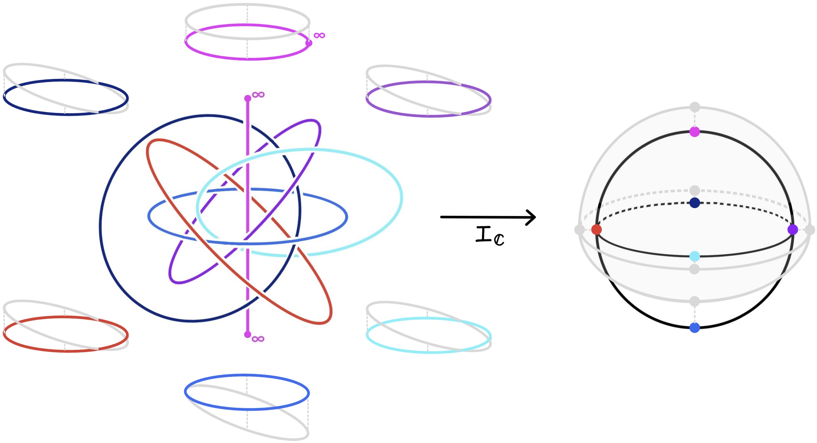
Spherical and complex projective designs can be related by the construction introduced by König [19, Corollary 1] and further investigated by Kuperberg [20, Theorem 4.1] which builds a -design on by placing the vertices of a regular -gon on each fiber of the complex projective map associated to a -design on . A related construction which builds a -design on by placing the vertices of a regular -gon on each fiber of the Hopf map associated to a -design on was—inspired by the independent observation of the construction of König by Cohn, Conway, Elkies, and Kumar [8, Section 4]—verified by Okuda [25, Theorem 1.1]. We generalize these results to prove Theorem 1.1, whose main consequence is that one can build a spherical -design by placing a spherical -design on each fiber of the projective or generalized Hopf map associated to a -design on a quotient real, complex, quaternionic, or octonionic projective space or sphere. This gives new constructions of -designs on from -designs on and -designs on for any , -designs on from -designs on and -designs on , and -designs on from -designs on or and -designs on .
Theorem 1.1 (Main Theorem).
For the reals , complex numbers , quaternions , or octonions and , take to be either the -projective map
| (1) |
for ( if ) or the -Hopf map
| (2) |
For weighted 0-designs on and on alongside base points for each , we consider
| (3) |
For any , is a weighted -design on if is a weighted -design on . Moreover, is a weighted -design on if is a weighted -design on and is a weighted -design on for each . If is constant in , the corresponding statements for unweighted designs (weighted designs with constant weight function) hold.
An interesting consequence of two applications of Theorem 1.1 is that, for the reals, complex numbers, or quaternions and , we can build a -design on by placing a -design on for each point of a -design on as in (3).
We define the objects of interest in Subsection 1.1. We then prove the projective settings of Theorem 1.1 in Section 2 and use these results to verify the generalized Hopf settings of the theorem in Subsection 2.1. Finally, we provide examples—some of which are known to be optimally small—of unweighted spherical -designs built as in Theorem 1.1 and discuss the sense in which the constructions of the theorem are each asymptotically optimal as in Section 3.
1.1. Spaces, maps, and designs
Consider the real numbers , the complex numbers , the quaternions , and the octonions , which Hurwitz’s theorem [12, Section 10] states are exactly the normed division algebras over the real numbers. These algebras are respectively generated over by elements , , , and satisfying , for , and the relations illustrated by the Fano plane in Figure 1. While and are commutative and associative, is associative but noncommutative, and is noncommutative and nonassociative but alternative—i.e., for all , and [2].

Fix . By , , , and , we respectively denote the -dimensional real, complex, quaternionic, and octonionic vector spaces. is taken to be the -dimensional unit sphere in and is equipped with the uniform measure (meaning a measure on a metric space with respect to which any two balls of the same radius have the same measure) , which we abbreviate by and normalize such that . Then, picking
| (4) |
is the unit sphere in . We define the -dimensional (over ) -projective space —the space of -lines in —using a right action of multiplication, setting
| (5) |
Note that when , we may use the simpler presentation
by associativity of these algebras. We equip with the uniform measure , which we abbreviate by and normalize such that .
Our definition of is equivalent to the more common presentation
of discussed by Baez [2, Subsection 3.1]. Specifically, we can observe that , , and exactly when for using the fact that the subalgebra generated by any two elements of is associative, as can be seen from alternativity of combined with a lemma of Artin [26, Section 3]. Baez also discusses why it is sensible to consider octonionic projective spaces for exactly . The proofs in Section 2 do not directly apply to give a construction which builds a -design on from a -design on and -designs on because does not admit a presentation analogous to (5). Instead, they directly verify a construction which uses a map analogous to (1) from the set of triples satisfying to to relate -designs on to -designs on and -designs on preimages of .
Consider the -projective maps (1) and -Hopf map (2) as in Theorem 1.1. The measure we consider on is equivalent to the pushforward of the measure we consider on by the -projective map, as can be seen since will be uniform by symmetry and will be normalized such that . Additionally, we have , where
| (6) |
is a diffeomorphism identifying with . We note that , so we also have . Preimages of the -projective and -Hopf maps can be seen from (1) to each arise as the unit sphere in a subspace of of dimension 1 over . We equip these fibers with the uniform measure , which we normalize such that each fiber has volume 1.
The space of real-valued polynomials on is the closure of the constant and coordinate functions under addition and multiplication. We then say that is the space of polynomials of degree less than or equal to on ; i.e. polynomials whose terms are each the product of a constant function and at most coordinate functions. We then define
| (7) | |||
| (8) |
where is the pullback of by . We consider coordinates in for real-valued polynomials via the association which realizes as a -dimensional real vector space with basis vectors , the standard generators for the algebra over .
We do not use explicit spanning sets of polynomials on projective spaces in the proofs below, but note that Lyubich and Shatalova [22, Main Theorem] proved that for and where is the conventional inner product on , is spanned over by the functions
We now introduce weighted and unweighted -designs, numerical integration formulas (also known as quadrature or cubature rules) which precisely average polynomials of degree or less.
Definition 1.2.
Take to be a sphere or projective space , so we note . The pair of a finite subset and a function is called a weighted t-design on if
We may call a weighted spherical -design if is a sphere and a weighted -projective -design if is a -projective space. Additionally, is called an unweighted -design (or simply a -design) if is the constant function .

Literature discussing projective designs often defines these objects as finite subsets of projective spaces on which the averages of certain Jacobi polynomials vanish. It was proven by Lyubich [23, Proposition 2.2] that the projective settings of Definition 1.2 are equivalent to the definition more common in the literature. We note that the work of Lyubich has a typo: the word “tight” in their proposition should be omitted.
2. Validity of the constructions
In this section, we prove Theorem 1.1. We first verify Theorem 1.1 when is a projective map, then show in Subsection 2.1 that the cases of the projective settings give rise to the results of Theorem 1.1 when is a generalized Hopf map.
Proof of the projective settings of Theorem 1.1.
Taking , , and as in (4) along with , we consider weighted 0-designs on and on alongside base points for each . We then define as in (3).
Pick . Noting that for any and that is a 0-design on for each , we have
| (9) |
Additionally, we may observe from the definition (22) of that
| (10) |
Combining (9) and (10) with Definition 1.2, we see that is a weighted -design on exactly when
| (11) |
for all . Now, we also see from Definition 1.2 combined with the result
of Lemma 2.2 that (11) being satisfied for is exactly the condition that is a weighted -design on . Therefore, since we can see from the definition (8) of polynomials on projective spaces that
we have shown that is a weighted -design on if is a weighted -design on .
Now, say is a weighted -design on for each . Picking , (27) in Lemma 2.3 shows that for . So, applying a change of variables using (19) followed by the definition (22) of , we have that
for , which shows that
| (12) |
From (28) in Lemma 2.3, we see that , so combining (12) with (9) for gives us that
| (13) |
Additionally, we observe from (10) that
| (14) |
From (13) and (14), we see that (11) is satisfied for if it is satisfied for
so is a weighted -design on if is a weighted -design on . ∎
Elements of the proof of the projective settings of Theorem 1.1 were inspired by work of Okuda [25, Lemma 3.9] verifying the -Hopf setting of Theorem 1.1. We now prove facts cited in this proof. With , , , and as in (4), consider the left multiplication by a base point map
| (15) |
we define for each . Taking
| (16) |
along with
| (17) |
and respectively equipping these spaces with the restrictions of the measures and discussed in Subsection 1.1, we consider a local trivialization
| (18) |
of the -projective map, where we equip with the product measure .
Observe that pushes forward the uniform measure on to the uniform measure on ; i.e.
| (19) |
We now discuss how pushes forward the product measure on to the restriction of the uniform measure on to :
Lemma 2.1.
We have
| (20) |
Proof.
Similarly to as was done by Okuda [25, Lemma 4.2], we use (19) and (20) alongside Fubini’s theorem [14] to show that, with , , and as in (4), taking the average of any Lebesgue integrable function over provides the same result as taking the average on of the function which averages over each -projective fiber . For such and , recalling as in Subsection 1.1 that we normalize the measure on such that , we have
| (22) |
Lemma 2.2.
For , we have
| (23) |
Proof.
Pick and recall the definitions (16) and (17) of and respectively. We see using that has measure zero in followed by a change of variables using (20) in Lemma 2.1 that
| (24) |
Since and is the product measure on , Fubini’s theorem [14] followed by the fact that, taking for each , shows that
| (25) |
Changing variables using (19) and applying the definition (22) of alongside the fact that has measure zero in , we have
| (26) |
Combining (24), (25), and (26) then provides us with the desired result (23). ∎
Again consider , , , and as in (4) along with . We now discuss how as in (22) and the pullback operator induced by as in (15) relate polynomials.
Lemma 2.3.
We have
| (27) | |||
| (28) |
Proof.
Fix and consider
Extending to the map taking , the definition of polynomials on in Subsection 1.1 makes it clear that
The definition (7) of polynomials on spheres then shows (27).
Note that the definition (22) of shows that is the identity. Combining the definition of with this fact then shows that
To prove (28), we must then only show that , and the definition (8) of polynomials on shows that this will be true if
| (29) |
for all . Pick such to be a monomial of degree . We can observe from the description of multiplication of elements of in Subsection 1.1 that for any and ,
where and are monomials of degree on and respectively for all . Therefore, applying a change of variables for any base point using (19), we see that
Applying this fact, we see
Now, Lemma 2.4 shows that if , so (29) is satisfied, completing the proof. ∎
Lemma 2.4.
For any polynomial with terms having only odd degree, .
Proof.
Say is as in the statement of the lemma. We assume without loss of generality that is a monomial of odd degree . If , we have
for any . Now, take , so is even and thus is even for any . The antipodal map on has differential (the negative of the identity on ), so since
we see applying the change of variables that
because is a monomial of odd degree . So, we must have . ∎
2.1. The generalized Hopf settings
We show in this subsection that the results of Theorem 1.1 which use generalized Hopf maps to relate designs are equivalent to the cases of the corresponding projective settings verified in Section 2. To this end, pick , , and as in (4) and recall the diffeomorphism described in (6) which identifies with .
Lemma 2.5.
We have
Corollary 2.6.
is a weighted -design on if and only if is a weighted -design on .
Applying Corollary 2.6, the case of the -projective setting of Theorem 1.1 proves the corresponding -Hopf setting of the theorem.
Proof of Lemma 2.5.
For any , we note that
Therefore, for any , we have from the definition (22) of that
We can therefore see from definitions (2) of and (6) of that
| (30) |
We also can observe from the description of multiplication of elements of in Subsection 1.1 that
| (31) |
Combining (30) with (31) and (28) in Lemma 2.3, we see that
So, to complete the proof, we must only show that
| (32) |
which will in turn be true if
| (33) |
since applying to each side of (33) gives (32) by (30) and the fact we may observe from the definition (22) of that is the identity map. Fix and note that by the definition (8) of , so we may consider and constants for satisfying such that
Again since is the identity map, we see that is the identity on . Also note that this operator is linear. Defining
we therefore have that
| (34) |
Now, for any and as above, we see from Lemma 2.7 that there exists satisfying
Assume without loss of generality that . We may observe from the definition (1) of that
Lemma 2.4 then guarantees that must have terms of only even degree, so we must have for some . Therefore,
We thus have by the definition (2) of , showing by linearity of that . ∎
Lemma 2.7.
For , , and , if
| (35) |
for some , we have
| (36) |
for some .
Proof.
Consider as in the statement of the lemma and label . For any
we may apply a change of variables using (19) to see that
| (37) |
We then see from (35) that
| (38) |
The definition (1) of and the fact that then demonstrate that and . Combining this with (37) and (38), we can see that
| (39) |
Every (nonzero) term of must thus contain at least multiples of or and at least multiples of or , as (39) would otherwise not be satisfied when or . Now, we can observe from the definition (8) of and (28) in Lemma 2.3 that
so the degree of does not exceed . Therefore, every (nonzero) term of must contain exactly multiples of or and exactly multiples of or . This fact combined with (39) completes the proof. ∎
3. Examples and optimality
We now present examples of -designs on which can be built using the constructions communicated by Theorem 1.1, remark on the sizes of such -designs, and discuss the sense in which these constructions are asymptotically optimal as . Note that all examples provided using the complex Hopf or complex projective settings could also have been produced using the results of Okuda [25, Theorem 1.1] or König [19, Corollary 1] and Kuperberg [20, Theorem 4.1] respectively.
We use the fact that, for , the vertices
| (40) |
of a regular -gon are a -design on [10, Example 5.1.4]. We also note that we pick base points for the fibers of the -Hopf maps using the equation
| (41) |
We first discuss an example remarked on by Okuda [25, Example 2.4].
Example 3.1.
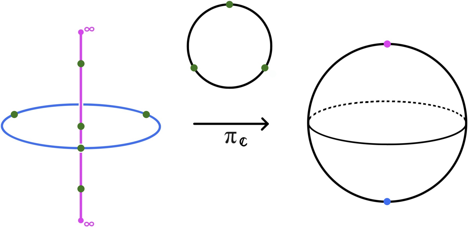
Example 3.2 presents a family of 7-designs on discussed by Cohn, Conway, Elkies, and Kumar [8]. These authors also discuss the example of the root system, a 5-design on which consists of four sets of points which are each the vertices of a hexagon inscribed in a Hopf fiber. These Hopf fibers have images under the Hopf map which are the vertices of a tetrahedron on , a 2-design [4, Example 2.7].
Example 3.2.
As discussed by Bannai and Bannai [4, Example 2.7], the vertices
of a regular octahedron on (pictured in Figure 2) constitute a -design. We also know that the vertices of a regular -gon are a -design on . The -Hopf setting of Theorem 1.1 then gives us that
is a -design for any base points . We may then use (41) to pick these base points, giving rise to a concrete family of 7-designs on . Figure 5 visually describes this example.
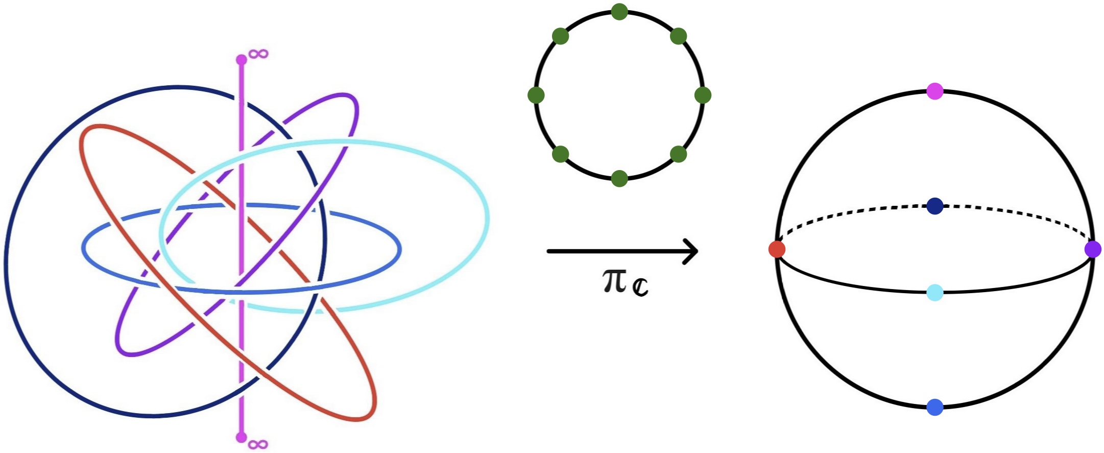
The 24-point 5-design and 48-point 7-design discussed by Cohn, Conway, Elkies, and Kumar [8] are putatively optimally small among designs on of their respective strengths. Table 1 details when -designs minimally small among those constructed as in the -Hopf setting of Theorem 1.1 have optimal size among all known -designs on .
| Putatively optimal minimum | |||
|---|---|---|---|
| 0 | 1 | 1 | 1 |
| 1 | 1 | 2 | 2 |
| 2 | 2 | 6 | 5 |
| 3 | 2 | 8 | 8 |
| 4 | 4 | 20 | 20 |
| 5 | 4 | 24 | 24 |
| 6 | 6 | 42 | 42 |
| 7 | 6 | 48 | 48 |
| 8 | 12 | 108 | 96 |
| 11 | 12 | 144 | 120 |
Also note that, as Chen, Frommer, and Lang computationally verified the existence of -designs on with points for [7], we may apply the -Hopf setting of Theorem 1.1 to verify existence of -designs on with points for .
Applying Corollary 2.6, we get examples of the complex projective setting of Theorem 1.1 from Example 3.1, Example 3.2, and the cases discussed in Table 1. We now give other examples of the projective settings of the theorem.
With , , , and as in (4) and
is a -design on for . This can be seen (when ) from the fact that a set is a 1-design on if
where is the identity on [9, Section 2].
Example 3.3.
As is (trivially) a -design on for any ,
is a -design on by the real projective setting of Theorem 1.1.
For , may similarly be built from the 1-design and the 3-design using the -projective construction of Theorem 1.1. The sets are known to be tight 3-designs [4], where a -design is called tight if it achieves the lower bound on the size of such a design provided by Delsarte, Goethals, and Seidel [10, Definition 5.13] in the spherical setting or the analogous bounds of Dunkl [11] and of Bannai and Hoggar [5, Proposition 1.1] in the projective setting.
A number of tight projective -designs were presented by Hoggar [17, Table 3] and Levenshtein compiled these and other projective designs into a list [21, Table 9.2]. Tight designs outlined by Hoggar include a 40-point 3-design on [17, Example 6], a 126-point 3-design on [17, Example 7], and a 165-point 3-design on [17, Example 9]. Noting that as in (40) is a tight t-design on for any [18, Theorem A] and that the 48-point 7-design on discussed by Cohn, Conway, Elkies, and Kumar [8] as an initial example of a design built as in the complex Hopf construction of Theorem 1.1 is conjectured to be an optimally small 7-design on [15, Table 1], we get from Theorem 1.1 a 320-point 7-design on , a 1,008-point 7-design on , and a 7,920-point 7-design on . While each of these designs is putatively optimally small among 7-designs on their respective spheres built using Theorem 1.1, these designs are not themselves tight—in fact, tightness is rare among designs built on as in Theorem 1.1 for .
Taking , , and as in (4) alongside and , say and are the minimal numbers of points required to form a -design on and on respectively. Work of Bondarenko, Radchenko, and Viazovska [6, Theorem 1] combined with the tightness bounds of Delsarte, Goethals, and Seidel [10, Theorems 5.11, 5.12] shows that as and work of Etayo, Marzo, and Ortega-Cerdà [13, Theorem 2.2] combined with the tightness bounds of Dunkl [11] shows that as . This demonstrates that each construction of Theorem 1.1 is asymptotically optimal as , in the sense that an optimally small -design capable of being built on by such a construction will have size
Acknowledgements
The author would like to thank Henry Cohn for suggesting this problem and providing helpful insights throughout the research process, as well as the reviewer for helpful comments. The author would also like to thank the School of Science, the Department of Mathematics, and the Office of Graduate Education for the MIT Dean of Science fellowship for support in their doctoral studies and would like to acknowledge NSF grant DMS-2105512 and the Simons Foundation Award #994330 (Simons Collaboration on New Structures in Low-Dimensional Topology) for their support.
References
- [1] (2000) A minimal design of order 11 on the three-dimensional sphere. Mat. Zametki 67 (4), pp. 489–497. External Links: ISSN 0025-567X,2305-2880, Document, Link, MathReview (Victor. A. Zinoviev) Cited by: Table 1.
- [2] (2002) The octonions. Bull. Amer. Math. Soc. (N.S.) 39 (2), pp. 145–205. External Links: ISSN 0273-0979,1088-9485, Document, Link, MathReview (Helena Albuquerque) Cited by: §1.1, §1.1.
- [3] (1992) Construction of spherical -designs. Geom. Dedicata 43 (2), pp. 167–179. External Links: ISSN 0046-5755,1572-9168, Document, Link, MathReview (J. J. Seidel) Cited by: §1.
- [4] (2009) A survey on spherical designs and algebraic combinatorics on spheres. European J. Combin. 30 (6), pp. 1392–1425. External Links: ISSN 0195-6698,1095-9971, Document, Link, MathReview (Bertrand Meyer) Cited by: §1, Example 3.2, §3, §3.
- [5] (1985) On tight -designs in compact symmetric spaces of rank one. Proc. Japan Acad. Ser. A Math. Sci. 61 (3), pp. 78–82. External Links: ISSN 0386-2194, Link, MathReview Entry Cited by: §1, §3.
- [6] (2013) Optimal asymptotic bounds for spherical designs. Ann. of Math. (2) 178 (2), pp. 443–452. External Links: ISSN 0003-486X,1939-8980, Document, Link, MathReview (Hiroshi Nozaki) Cited by: §1, §1, §3.
- [7] (2011-02) Computational existence proofs for spherical t-designs. Numer. Math. 117, pp. 289–305. External Links: Document Cited by: §3.
- [8] (2007) The root system is not universally optimal. Experiment. Math. 16 (3), pp. 313–320. External Links: ISSN 1058-6458,1944-950X, Link, MathReview Entry Cited by: §1, §3, §3, §3.
- [9] (2016) Optimal simplices and codes in projective spaces. Geom. Topol. 20 (3), pp. 1289–1357. External Links: ISSN 1465-3060,1364-0380, Document, Link, MathReview (Anton Vladimirovich Shutov) Cited by: §3.
- [10] (1977) Spherical codes and designs. Geom. Dedicata 6 (3), pp. 363–388. External Links: Document, Link, MathReview (Michel Deza) Cited by: §1, §1, Table 1, §3, §3, §3.
- [11] (1979) Discrete quadrature and bounds on -designs. Michigan Math. J. 26 (1), pp. 81–102. External Links: ISSN 0026-2285,1945-2365, Link, MathReview (D. K. Ray-Chaudhuri) Cited by: §1, §3, §3.
- [12] (1990) Numbers. German edition, Graduate Texts in Mathematics, Vol. 123, Springer-Verlag, New York. Note: With an introduction by K. Lamotke, Translation edited and with a preface by J. H. Ewing, Readings in Mathematics External Links: ISBN 0-387-97202-1, Document, Link, MathReview Entry Cited by: §1.1.
- [13] (2018) Asymptotically optimal designs on compact algebraic manifolds. Monatsh. Math. 186 (2), pp. 235–248. External Links: ISSN 0026-9255,1436-5081, Document, Link, MathReview Entry Cited by: §1, §3.
- [14] (1907) Sugli integrali multipli. Rom. Acc. L. Rend. (5) 16 (1), pp. 608–614 (Italian). External Links: ISSN 0001-4435 Cited by: §2, §2.
- [15] (2003) Spherical designs in four dimensions. In Proceedings 2003 IEEE Information Theory Workshop, pp. 253–258. External Links: Document Cited by: Table 1, §3.
- [16] (1996) McLaren’s improved snub cube and other new spherical designs in three dimensions. Discrete Comput. Geom. 15 (4), pp. 429–441. External Links: ISSN 0179-5376,1432-0444, Document, Link, MathReview (J. J. Seidel) Cited by: Table 1.
- [17] (1982) -designs in projective spaces. European J. Combin. 3 (3), pp. 233–254. External Links: ISSN 0195-6698,1095-9971, Document, Link, MathReview Entry Cited by: §3.
- [18] (1982) On spherical -designs in . European J. Combin. 3 (3), pp. 255–258. External Links: ISSN 0195-6698,1095-9971, Document, Link, MathReview (J. J. Seidel) Cited by: §3.
- [19] (1999) Cubature formulas on spheres. In Advances in multivariate approximation (Witten-Bommerholz, 1998), Math. Res., Vol. 107, pp. 201–211. External Links: ISBN 3-527-40236-5, MathReview Entry Cited by: §1, §3.
- [20] (2006) Numerical cubature from Archimedes’ hat-box theorem. SIAM J. Numer. Anal. 44 (3), pp. 908–935. External Links: ISSN 0036-1429,1095-7170, Document, Link, MathReview Entry Cited by: §1, §3.
- [21] (1992) Designs as maximum codes in polynomial metric spaces. Vol. 29, pp. 1–82. Note: Interactions between algebra and combinatorics External Links: ISSN 0167-8019,1572-9036, Document, Link, MathReview (Michael Klemm) Cited by: §3.
- [22] (2005) Polynomial functions on the classical projective spaces. Studia Math. 170 (1), pp. 77–87. External Links: ISSN 0039-3223,1730-6337, Document, Link, MathReview (Walter Schempp) Cited by: §1.1.
- [23] (2009) On tight projective designs. Des. Codes Cryptogr. 51 (1), pp. 21–31. External Links: ISSN 0925-1022,1573-7586, Document, Link, MathReview Entry Cited by: §1.1.
- [24] (1981) Combinatorial configurations in terms of distances. Memorandum Technical Report 81-09 (Wiskunde), Eindhoven University of Technology. Cited by: §1.
- [25] (2015) Relation between spherical designs through a Hopf map. Note: Preprint, arXiv:1506.08414 Cited by: §1, §2, §2, §3, §3.
- [26] (1995) An introduction to nonassociative algebras. Dover Publications, Inc., New York. Note: Corrected reprint of the 1966 original External Links: ISBN 0-486-68813-5, MathReview Entry Cited by: §1.1.
- [27] (1984) Averaging sets: a generalization of mean values and spherical designs. Adv. in Math. 52 (3), pp. 213–240. External Links: ISSN 0001-8708, Document, Link, MathReview (J. J. Seidel) Cited by: §1, §1.
- [28] (2018) Efficient spherical designs with good geometric properties. In Contemporary computational mathematics—a celebration of the 80th birthday of Ian Sloan, pp. 1243–1285. External Links: ISBN 978-3-319-72455-3; 978-3-319-72456-0, MathReview Entry Cited by: Table 1.