A catalogue of Galactic GEMS: Globular cluster Extra-tidal Mock Stars
Abstract
This work presents the Globular cluster Extra-tidal Mock Star (GEMS) catalogue of extra-tidal stars and binaries created via three-body dynamical encounters in globular cluster cores. Using the particle-spray code Corespray, we sample extra-tidal stars and escaped recoil binaries for 159 Galactic globular clusters. Sky positions, kinematics, stellar properties and escape information are provided for all simulated stars. Stellar orbits are integrated in seven different static and time-varying Milky Way gravitational potential models where the structure of the disc, perturbations from the Large Magellanic Cloud and the mass and sphericity of the Milky Way’s dark matter halo are all investigated. We find that the action coordinates of the mock extra-tidal stars are largely Galactic model independent, where minor offsets and broadening of the distributions between models are likely due to interactions with substructure. Importantly, we also report the first evidence for stellar stream contamination by globular cluster core stars and binaries for clusters with pericentre radii larger than five kiloparsecs. Finally, we provide a quantitative tool that uses action coordinates to match field stars to host clusters with probabilities. Ultimately, combining data from the GEMS catalogue with information of observed stars will allow for association of extra-tidal field stars with any Galactic globular cluster; a requisite tool for understanding population-level dynamics and evolution of clusters in the Milky Way.
keywords:
galaxies: star clusters – globular clusters: individual – stars: kinematics and dynamics – software: simulations1 Introduction
Globular clusters (GCs) are densely packed spherical collections of stars. Current observations find the existence of over GCs in our Milky Way, with complete orbital and structural parameters available in catalogues like Harris (1996), Baumgardt & Hilker (2018) and Vasiliev (2019). Recent data releases from the European Space Agency satellite Gaia (Gaia Collaboration et al., 2016) and the Apache Point Observatory Galactic Evolution Experiment (APOGEE; Abdurro’uf et al., 2022), have also revolutionized our understanding of GC properties. For instance, Gaia has allowed for exquisite and precise kinematic measurements of cluster stars (Gaia Collaboration et al., 2018), while APOGEE chemical abundances have been pivotal in identifying multiple stellar populations in GCs (e.g. Schiavon et al., 2017; Masseron et al., 2019; Mészáros et al., 2020). However, while much progress has been made to understand GCs in the present-day, probing cluster formation and evolution is challenging as GCs lose knowledge of their birth conditions as they lose stars and undergo structural changes over time.
1.1 Three-body encounters in globular clusters
Escaped stars from GCs inform a myriad of astrophysics; including cluster dynamics, binary fractions and star formation histories. GCs lose mass through a variety of mechanisms, with Weatherford et al. (2023) providing a comprehensive overview of stellar escape processes. While cluster evaporation and tidal stripping are the dominant channels for stellar escape from a GC, these methods primarily eject low-mass stars that have segregated to the outskirts of the cluster, yielding the creation of stellar streams or tidal tails. Since mass segregation causes high-mass stars and binaries to sink to a cluster’s core, dynamical interactions in the core also must be considered to learn about high-mass stellar ejection, GC core evolution and the processes that ultimately produce isolated cluster field stars and binaries.
One of the most common dynamical interactions in a GC core is a three-body encounter. Although the exact interaction rate depends on cluster core density and mass, three-body encounters typically occur once every Myr in a GC (Leigh & Sills, 2011). For GC binary fractions greater than 10, three-body encounters will even occur more frequently than binary-binary interactions (Leigh & Sills, 2011). In a three-body interaction, three stars will experience a close gravitational encounter, wherein a single star is ejected and the other two stars become a recoil binary system (for a complete review of three-body dynamics, see Valtonen & Karttunen, 2006). During the encounter, both the single star and recoil binary will experience a velocity kick as the binary hardens. The magnitude of the kick depends on the configuration of stellar masses, positions, and velocities, where stars can either be retained in the cluster or escape entirely (e.g. Leigh et al., 2023). If the velocity kick is especially large and the stars travel beyond the tidal radius of the GC, the stars will become extra-tidal in nature.
Since three-body interactions will continuously occur as the GC evolves, extra-tidal stars and binaries will be ejected at random times during a GC’s orbit around the Galaxy. Coupled with the fact that the mass of the star/binary and the magnitude of the velocity kick will change for different three-body encounters, extra-tidal stars and binaries from a given cluster could be distributed all throughout the Milky Way. Unfortunately, the various initial configurations and interactions with Galactic sub-structures (e.g. orbiting through the Galactic disc or halo, experiencing dynamical perturbations from the Large Magellanic Cloud, etc.) make associating extra-tidal stars to birth clusters difficult.
1.2 Chemo-dynamical tagging to associate stars with clusters
Fortunately, recent data releases by surveys like APOGEE have allowed for the advent of “chemical tagging”: a method which utilizes chemical abundances to associate chemically similar stars with their birth environments. While chemical tagging has been an excellent tool to identify field stars that were likely born in the same birth cluster (e.g. Kos et al., 2018; Price-Jones et al., 2020), chemistry alone does not definitively indicate that the stars originated in the same GC (Ness et al., 2018, 2019; Casamiquela et al., 2021). However, since most stars in a GC are born from the same giant molecular cloud, they will not just share similar abundances, but kinematics as well. Thus, “chemo-dynamical tagging” (associating stars via their chemistry and stellar kinematics) is a useful tool to identify stellar birth environments with higher confidence (e.g. Chen et al., 2018; Hanke et al., 2020; Webb et al., 2020).
Chemo-dynamical tagging has also been used to identify extra-tidal field stars of GCs, with Chun et al. (2020) combining APOGEE DR14 abundances and radial velocities to identify new extra-tidal stars around the Galactic GCs M53 and NGC 5053. In Grondin et al. (2023), we developed a new method to identify extra-tidal stars produced via three-body encounters in GC cores, using M3 as a case study. With APOGEE DR17 chemistry and radial velocities, Grondin et al. (2023) identified 103 extra-tidal candidates of M3 through application of the t-Stochastic Neighbour Embedding (t-SNE; Van der Maaten & Hinton, 2008) and Uniform Manifold Approximation and Projection (UMAP; McInnes et al., 2018) dimensionality reduction algorithms. To confirm whether each candidate indeed originated from a three-body encounter in M3’s core, we developed Corespray: a Python-based particle spray code simulating extra-tidal stars from Galactic GCs. Corespray’s ability to quickly sample three-body interactions makes it an ideal tool to investigate the spatial, kinematic and stellar characteristics of dynamically-created extra-tidal stars and binaries on a large scale.
While Grondin et al. (2023) were successful at identifying 10 new extra-tidal stars of one Galactic GC, a catalogue containing mock extra-tidal star and binary data for all Galactic GCs allows for an even deeper exploration into the evolution of Galactic GCs and the Milky Way as a whole. For instance, kinematic distributions could be used to associate field extra-tidal stars with birth clusters, allowing for identification of extra-tidal single star and binary pairs. Moreover, Cabrera & Rodriguez (2023) suggest that dynamical interactions in GC cores could yield hyper-velocity or runaway stars in the Milky Way, where a catalogue of extra-tidal stars could be used to trace observed stars back to clusters.
1.3 This work
In this study, we present the Globular cluster Extra-tidal Mock Star (GEMS) catalogue. The GEMS sample represents the first simulated mock catalogue of extra-tidal stars and binaries created via three-body encounters in Galactic GC cores. We simulate extra-tidal star and binary spatial (on-sky positions, distances), kinematic (proper motions, radial velocities, action coordinates) and stellar information (masses, escape velocities) for all 159 Galactic GCs listed in Baumgardt & Hilker (2018) using Corespray. In Section 2, we describe Corespray and outline the initial simulation set-up and input parameters considered in this study. Spatial and kinematic distributions for both the single extra-tidal stars and recoil binaries of all GCs are presented in Section 3, with the results discussed in Section 4. Section 4 also presents a new quantitative tool that uses extra-tidal star action coordinates to match field stars with host GCs, where the code is available in Appendix D. In combination with chemo-dynamical data from APOGEE and Gaia, the GEMS catalogue aims to act as a resource for understanding population-level dynamics and evolution of GCs in the Milky Way.
2 Simulating extra-tidal stars with Corespray
2.1 The Corespray particle spray code
To construct our extra-tidal star and binary distributions, we use the particle spray code Corespray111For a complete outline of how Corespray works, please refer to Grondin et al. (2023) or visit https://github.com/webbjj/corespray for download and usage instructions. (Grondin et al., 2023). Using the theoretical three-body dynamics framework presented in Valtonen & Karttunen (2006), Corespray samples three-body interactions in GC cores until single stars have travelled beyond the cluster’s tidal radius. Running Corespray requires the definition of GC orbital and structural parameters. Specifically, each cluster’s orbit is defined from its sky position, distance, proper motion and radial velocity. Structural parameters (i.e. mass, tidal radius, core density, velocity dispersion and escape velocity) are also essential for initializing each cluster and its unique escape criteria. Importantly, Corespray also takes in parameters like cluster orbital period, a number of extra-tidal stars to sample, a separation radius for core stars that experience three-body encounters, a stellar mass function and a model for the Galactic potential. Each of these parameters are defined by the user.
Once the aforementioned initial conditions are inputted, Corespray generates extra-tidal stars at random times along a cluster’s orbit throughout the Galaxy. Spatial (e.g. right ascension and declination, distance), kinematic (e.g. proper motions, radial velocities, action coordinates) and stellar (e.g. masses) information is produced for each single and binary escaper, allowing orbits to be integrated with galpy (Bovy, 2015) and large distributions of escapers to be produced.
While N-body integrators like Nbody6 (Aarseth, 2003), -GRAPE (Harfst et al., 2007), and PeTar (Wang et al., 2020) directly model three-body interactions in cluster cores, simulating the evolution of realistic globular clusters is computationally expensive due to their large particle numbers and old ages (Wang et al., 2016). Complicated by the fact that the birth properties of a given GC are needed to simulate its evolution to the present-day (Heggie, 2014), the prospect of producing a suite of direct -body simulations of the Milky Way’s GC population remains daunting. To study the outcomes of three-body interactions within GCs, many randomizations of each Galactic cluster would need to be completed, adding further to the study’s computational expense. Corespray’s abilities to quickly sample and integrate orbits for extra-tidal stars and binaries of any Galactic GC makes it an ideal tool to generate statistically significant distributions of escaped stars throughout the Milky Way.
2.2 Generating mock extra-tidal stars
2.2.1 Defining globular cluster parameters
In this study, GC structural parameters are obtained from the Baumgardt & Hilker (2018) GC catalogue 222All fundamental Galactic GC parameters can be accessed via the online database at https://people.smp.uq.edu.au/HolgerBaumgardt/globular/.. All GC orbital parameters are obtained from Baumgardt et al. (2019), Baumgardt & Vasiliev (2021) and Vasiliev & Baumgardt (2021). To define a tidal radius () boundary (and thus a threshold for where the star or binary will have officially ”escaped” the cluster), we use the Webb et al. (2013) at perigalacticon to compute the at apogalacticon. This definition ensures that we are only considering stars that are beyond at all points in the GC’s orbit through the Galaxy as being extra-tidal. Furthermore, since Corespray uses a combined Galactic and King potential to encompass influences from both the Milky Way and the GC itself, we must define a King-model central potential parameter () for each GC. From Harris (1996), the King-model central concentration parameter () can be obtained using the previously defined and core radii () presented in Baumgardt & Hilker (2018) via . The conversion from to is then performed using clustertools333For a complete description of clustertools capabilities and installation instructions, please visit https://github.com/webbjj/clustertools. (Webb et al., 2022) and data from gridfit (McLaughlin et al., 2008).
Another essential GC parameter to consider is the time period over which extra-tidal stars are simulated. Contrary to Grondin et al. (2023) who searched for recently escaped extra-tidal stars of M3, this study wishes to examine if/how the properties of extra-tidal stars and binaries evolve as a function of time. As such, for the purposes of this catalogue we generate stars that escape during random times along five orbital periods (Porb) of the GC through the Galaxy. The choice to simulate 5 orbital periods of escape is motivated by computational expense, as simulation time must be balanced against the number of extra-tidal stars being generated 444Simulating escape over more than 5 orbital periods is entirely possible within Corespray and should be considered for users interested in longer escape times.. To determine the Porb of each GC, we compute both the radial and azimuthal orbital periods using galpy (Bovy, 2015). Each Porb used in this study represents the maximum of the two computed cluster periods. It is important to note that 14 GCs in our sample (AM 1, Arp 2, BH 140, Crater, Eridanus, NGC 2419, Pal 3, Pal 12, Pal 14, Pyxis, Sagittarius II, Ter 7, Ter 8 and Whiting 1) have Porb Gyr. Consequently, this could result in stellar escape times where tesc Porb corresponds to times older than the age of the Universe. To ensure our distributions for these clusters are physical, we impose upper escape time boundaries of tesc Gyr, where 12 Gyr represents an intermediate age for the GCs in the Milky Way (Forbes & Bridges, 2010).
It is important to note that in this study, we assume a cluster’s properties remain constant over the course of five orbital periods. However for GCs with long orbital periods, this assumption is incorrect. Cluster cores get denser as they evolve towards core collapse (Heggie & Hut, 2003), so it is likely that clusters had lower central densities in the past. Lower central densities and velocity dispersions would result in three-body interactions that yield weaker kicks, potentially causing our distributions of extra-tidal stars to be wider for stars that escape later. This situation is of course complicated by the evolution of a cluster’s binary star population and tidal field. Hence, for an in-depth analysis of a specific GC’s extra-tidal star history, one may consider pairing Corespray with a cluster’s evolution track as generated via a fast-code prescription (e.g. the Evolve Me A Cluster of StarS (EMACSS) code; Alexander & Gieles, 2012) or a completed simulation of the internal dynamics (e.g. the Cluster Monte Carlo (CMC) code; Rodriguez et al., 2022).
2.2.2 Defining three-body encounter parameters
In addition to GC structural and orbital parameters, Corespray offers a variety of other tunable inputs to address specific science questions. We outline our choices for (i) the number of extra-tidal stars simulated, (ii) the binding energy of the binary (iii) the separation radius between the binary and single star during the three-body encounter and (iv) the stellar initial mass function (IMF) below.
First, since a goal of this study is to produce complete parameter spaces of extra-tidal stars and their recoil binaries, we choose to sample single escapers for each GC. Importantly, the fraction of recoil binaries that escape a cluster is dependent on individual GC characteristics and masses of the stars in the three-body encounter. Thus, high- distributions allow us to completely explore the parameter spaces of escaped single extra-tidal stars, while also producing a statistically significant sample of escaped recoil binaries. It is important to note here that in generating a statistically significant sample of ET stars we do not assume or calculate a three-body interaction rate for the GCs. Sub-sampling the distribution of ET stars based on a given clusters three-body interaction rate would allow for a single realization of where a given clusters ET stars could be located.
Second, in order for the three-body interactions simulated with Corespray to reflect the interactions that occur in GCs, we assume a cluster’s binary star binding energy distribution follows Opik’s Law (a distribution with power-law slope of -1). Hence, interactions with soft binaries will be sampled more frequently than interactions with hard binaries, which reflects what is expected in actual GCs (Leigh et al., 2022).
Third, to allow for different configurations of three-body encounters, we sample a variety of separation radii between the single star and binary during each interaction. Specifically, we randomly sample separation radii between the semi-major axis of the binary and twice the mean separation of stars in the GC’s core. Since only encounters that lead to escaped stars are modelled, setting such a large upper bound on the separation radius ensures we cover the entire range of possible interactions albeit with increased computational expense.
Finally, initializing three-body encounters requires assigning masses to each component of the system. While sampling from a IMF allows us to probe a variety of mass configurations, defining an IMF to model mass distributions in GC cores is challenging. This is because (i) the high stellar core number density makes it difficult to observe individual stars and (ii) many clusters contain dark compact objects (i.e. neutron stars and black holes), which despite significantly contributing to the mass distribution, would remain observationally unresolved. Furthermore, mass segregation and tidal stripping over billions of years would remove many low mass cluster stars, shifting the core mass distribution to an overall higher average stellar mass. To mitigate some of these challenges, we sample masses from a Kroupa (2001) IMF containing stars. This IMF is then evolved for 12 Gyr with McLuster (Küpper et al., 2011) to incorporate some of the aforementioned effects and ultimately obtain a realistic estimate for GC stellar mass distributions at the present-day. It is important to note that the components of the binaries will also evolve towards a top-heavy IMF over time, which is not accounted for in this set-up. While this is a caveat of the initialized three-body encounters, the GEMS catalogue could be sampled to focus on stars over a given mass range, allowing for an examination into the results of interactions featuring heavier binary mass configurations.
2.3 Galactic potential models
In the last few decades, significant attention has been paid towards understanding our Milky Way’s gravitational potential (e.g. Koposov et al., 2010; Irrgang et al., 2013; Bovy & Rix, 2013; Bovy, 2015; McMillan, 2017; Malhan & Ibata, 2019; Eadie & Jurić, 2019). The precise potential of the Galaxy still remains an open question (for a comprehensive discussion of the structural properties of the Milky Way, see Bland-Hawthorn & Gerhard, 2016), where different components of the Galaxy can influence the orbits of stars in a variety of different ways. For instance, recent observations have shown that non-axisymmetric structures like a bar can play an important role of the dynamics and structure of clusters and stars in and around the Galactic disc (e.g. Hattori et al., 2016; Price-Whelan et al., 2016; Pearson et al., 2017; Banik & Bovy, 2019; Thomas et al., 2023). Furthermore, studies have shown that the Large Magellanic Cloud could cause perturbations to the Milk Way halo (e.g. Garavito-Camargo et al., 2019; Erkal et al., 2021), additionally impacting the orbits of stars. Moreover, the mass and shape of the halo – where GCs primarily spend their time – are poorly constrained. Hence, it is essential to consider a variety of potential models when exploring the locations and kinematics of GCs and their extra-tidal stars over long periods of time. In this study, we simulate extra-tidal stars/binaries in seven different potential models:
-
1.
A 3-component static potential (MWPotential2014 in Bovy, 2015)
-
2.
MWPotential2014 + a disc with a rotating bar and transient-wave spiral arms
-
3.
A 6-component static potential with a heavy halo (McMillan17 in McMillan, 2017)
-
4.
MWPotential2014 + varying halo shapes:
-
•
Oblate halo,
-
•
Spherical halo,
-
•
Prolate halo,
-
•
-
5.
MWPotential2014 + infall of the Large Magellanic Cloud
Each Milky Way model is described in detail below, however for complete model descriptions, please refer to the referenced original studies and codes.
2.3.1 Baseline: a static tidal field
A simple model for the Milky Way’s potential is MWPotential2014 (Bovy, 2015). MWPotential2014 contains three main components: an exponentially cut-off power-law density profile to model the Galactic bulge, a Miyamoto & Nagai (1975) disc and a Navarro-Frenk-White dark matter halo (Navarro et al., 1996), with the model itself fit to Milky Way data (Bovy, 2015). Despite its utility, the default version of this model (i) is time-independent, (ii) contains a lower than expected halo mass based on recent observations (Posti & Helmi, 2019; Deason et al., 2021; Bird et al., 2022) and (iii) has a slightly lower circular velocity at the Solar radius than preferred by modern measurements (e.g. Eilers et al., 2019). Since we are interested in examining extra-tidal star characteristics across a variety of orbital periods and locations in the Galaxy, additional investigation into large scale structure, time-dependent potential evolution and halo structure is necessary. Regardless, MWPotential2014 is used as a baseline in this study.
2.3.2 Disc: a rotating bar + transient-wave spiral arms
Although GCs spend much of their time in the Galactic halo, interactions with the Galactic disc also occurs during their orbits through the Galaxy. As extra-tidal stars and binaries are ejected at random times during a cluster’s orbit, it is possible that large-scale interactions with the disc could influence an extra-tidal star’s orbital properties. While direct observational evidence for a central bar at the centre of the Milky Way has been known for many decades (Blitz & Spergel, 1991), the formation and evolution of the Galaxy’s spiral arms is more uncertain. Historically, it has been thought that the spiral arms of the Milky Way originally formed through “density waves” – overdense, rotating regions of space (for an in-depth review of the history of spiral structure, see Shu, 2016). However, recent observational studies have favoured transient-wave spiral arms, which are spiral arms that grow and decay over time with radially dependent rotational rates. For instance, Castro-Ginard et al. (2021) use Gaia EDR3 data to find that different pattern speeds are better aligned with transient spirals than typical density waves.
As such, we modify our baseline MWPotential2014 potential to incorporate a rotating Galactic bar from Dehnen (2000), with evolving spiral arms from Hunt et al. (2019) – henceforth known as the “Bar+Transient Wave” potential555This Bar+Transient Wave potential model featuring large-scale structure in the Milky Way disc has been integrated into Corespray, where further description of how to implement this time-dependent potential is available at https://github.com/webbjj/corespray/tree/main/corespray/potential.. Notably, this potential model is time-dependent, where the first two transient arms are initialized at a time equal to 1 Gyr before the start of the simulation. One arm is initialized with an amplitude of zero in density-space while the other arm is at maximum amplitude. The spiral arms then continue to grow and decay over the evolution of the cluster. The lifetime of a given arm is 460 Myr and the initialization is such that there are always two active arms, with one reaching maximum every 230 Myr (Hunt et al., 2019).

2.3.3 Halo: a static tidal field with a heavy dark matter halo
As many GCs spend the majority of their orbits in the Galactic halo, it is important to consider a range of halo potentials when simulating extra-tidal stars and binaries. Unfortunately, constraining the mass of the Galactic dark matter halo is difficult, as measurements are typically extrapolations from the luminous matter in our Galaxy. To incorporate a more complex gravitational potential that features a more realistic halo mass, we use the McMillan (2017) model. This potential models the Milky Way using six components (as opposed to three in MWPotential2014) and is fit to modern kinematic data. Importantly, the McMillan (2017) potential model contains a larger virial mass compared to MWPotential2014 ( versus , respectively). Conveniently, the McMillan (2017) potential is also implemented in galpy (Bovy, 2015) as McMillan17.
2.3.4 Halo: a non-spherical dark matter halo
We also examine whether our extra-tidal star distributions are influenced by the triaxiality of the Milky Way’s dark matter halo. The shape of the dark matter halo is typically quantified by the flattening parameter , the ratio of the axis scale length in the disk plane versus the polar axis (). A value of represents complete sphericity of the dark matter halo, whereas implies an oblate halo and corresponds to a prolate halo. The Milky Way’s dark matter halo shape is currently poorly constrained, thus we consider three different values of that span a variety of values: (i) (Vera-Ciro & Helmi, 2013, who determine by fitting properties of the Sagittarius stellar stream), (ii) (Palau & Miralda-Escudé, 2023, who determine via the stellar streams of NGC3201, M68, and Palomar 5) and (iii) (Posti & Helmi, 2019, who determine via proper motions of 75 GCs from Gaia DR2 and 25 GCs from the Hubble Space Telescope). For simplicity, we do not consider disk-plane non-axisymmetry () or tilting of the dark matter halo. This assumption is reinforced by theoretical arguments which posit that baryonic disk growth encourages the dark halo to align with the disk plane and become axisymmetric, a picture backed up by evidence from simulations (e.g. Dubinski, 1994; Abadi et al., 2010; Kazantzidis et al., 2010).
Once again, we define a 3-component Galactic potential model, where the bulge and disc components are the same as in our baseline (MWPotential2014), however we adopt a TriaxialNFWPotential (normalize=0.35) with default components in galpy (Bovy, 2015). The only thing that is varied between each run is the flattening parameter . Since each value corresponds to a new Galactic potential model, a subset of three GCs is chosen to probe a representative range of Galactocentric distances while minimizing computational expense. Since triaxiality effects would be stronger for clusters located in the Galactic halo, we select (from Baumgardt & Hilker, 2018) halo clusters M3 ( kpc), Palomar 5 ( kpc) and Pyxis ( kpc) as our test GCs.
2.3.5 Halo: perturbations from the Large Magellanic Cloud
Recent observations and simulations have shown that the Large Magellanic Cloud (LMC) exhibits a gravitational pull on the Milky Way, causing both a dynamical wake and non-inertial Galactocentric reference frame (e.g. Garavito-Camargo et al., 2019, 2021; Conroy et al., 2021; Erkal et al., 2021; Vasiliev, 2023). Moreover, these studies suggest that the infall of the LMC could cause dynamical perturbations to the Milky Way’s stellar and dark matter halos, causing GCs – and ejected stars thereof – orbiting near the LMC to experience kinematic perturbations. Thus, we define a non-inertial frame force due to the LMC in galpy (Bovy, 2015), where the exact model used is described in detail at https://docs.galpy.org/en/v1.7.2/orbit.html#orbit-example-lmc-dynfric and added to our baseline MWPotential2014.
3 Results
As outlined in Section 2, we simulate 50,000 extra-tidal stars and corresponding recoil binaries in five different Galactic potential models for 159 GCs in Baumgardt & Hilker (2018) using Corespray. Each extra-tidal star and binary contains complete spatial (e.g. right ascension, declination, distance), kinematic (e.g. proper motions and radial velocities) and stellar (e.g. masses) information, allowing for an investigation into an array of different characteristics. Escape times and velocities of each star are also known, allowing for an examination into how the extra-tidal distributions change with time. Below, we highlight the outcomes of extra-tidal stars/binaries simulated in the baseline static tidal field (MWPotential2014), where the catalogue itself is available online at https://zenodo.org/record/8436703. Note that we ignore observational uncertainties on the cluster phase-space coordinates, however one could account for this by running several iterations of a specific cluster with Corespray.
3.1 Extra-tidal single star properties
3.1.1 Spatial distributions
To examine how extra-tidal stars from three-body encounters in GC cores are distributed throughout the Milky Way, we show the Corespray spatial distributions of all single extra-tidal stars for each cluster in Baumgardt & Hilker (2018) in Figure 1. It is clear that extra-tidal stars can end up far from their original parent cluster, with distribution shapes widely varying. Elongated extra-tidal star streams are typically observed in clusters that have pericentre radii () larger than five kiloparsecs (bottom right panel of Figure 1). Of the 31 clusters in Baumgardt & Hilker (2018) that have kpc, more than half have extremely low cluster escape velocities, with km/s. Generally, these clusters also have lower core densities and higher core radii compared to clusters with kpc, potentially allowing the extra-tidal stars to more easily escape the cluster altogether. This stream-like behavior is contrary to clusters with kpc (bottom left panel of Figure 1), where extra-tidal stars typically congregate around each GC’s centre. Clusters with small typically have shorter orbital periods compared to clusters in the halo. Hence, stars that escape these clusters will drift away from the progenitor cluster faster and are more likely to end up dispersed all throughout the Galaxy. Thus, the only structure that is observed for these clusters is a concentration around the cluster itself. In combination with GC structural properties, the cluster’s orbit and subsequent interaction with Galactic substructure could also influence the overall shape of each extra-tidal star distribution.
3.1.2 Action distributions


Generally, GC stars have similar kinematic properties (i.e. proper motions, radial velocities), as they are born from the same collapsing and rotating giant molecular cloud. However extra-tidal stars are the result of dynamical interactions, which impart velocity kicks onto each escaper and thus change the overall kinematics of the systems. Post-cluster escape, extra-tidal stars can also interact with large scale Galactic substructure, further altering the kinematics of the stars. Combined with unique three-body encounter configurations (i.e. masses and initial separations) and locations of ejection, extra-tidal stars from one GC could thus exhibit a range of kinematics, often much different than those of the host cluster itself. To further complicate things, proper motions and radial velocities of both a GC and its escaped stars will change with orbital phase, making it difficult to establish star-cluster associations using non-conserved kinematic quantities alone.
To navigate this issue, we compute actions – canonical momenta which are, in principle, conserved along orbit trajectories (see Chapter 3.5 of Binney & Tremaine, 2008, for a review) – for our samples of extra-tidal stars. Actions and (Note is trivial) are computed using the “Stäckel fudge” technique of Binney (2012), implemented in galpy as described by Mackereth & Bovy (2018). For each star, we compute the appropriate focal length for the Stäckel potential at its present-day coordinates following Sanders (2012). Many authors have tested the accuracy of the Stäckel approximation for realistic Galactic potentials by comparing with integrated orbits, usually finding it to be better than , and often about (e.g. Binney, 2012; Sanders, 2012; Bovy, 2015; Mackereth & Bovy, 2018; Lane et al., 2022). The approximation is best for disc-plane orbits, and tends to be worse for highly eccentric orbits, those which venture near the Galactic poles, or those in the bulge.
The three actions are often concisely displayed on a 2D plane with on the horizontal axis and on the vertical axis (Myeong et al., 2019; Vasiliev, 2019; Lane et al., 2022). Here, is the normalizing total action (note that and are manifestly positive). When actions are presented and scaled in this way, a characteristic diamond boundary defines the edges of the space, leading to its common name: the ‘action diamond’. The action diamond is useful in that it efficiently communicates the shape and orientation of an orbit, but can be limiting because its scale-free nature leads to degeneracies among orbits with similar shapes and orientations but different energies or radii. Nonetheless it is a valuable tool for studying associations among Galactic structures (Myeong et al., 2019; Vasiliev, 2019), hence our choice in employing it here to study the dynamical similarities and differences between ejected GC stars.
Figure 2 shows the action diamond for extra-tidal stars of all GCs in Baumgardt & Hilker (2018). For clarity, we only plot the actions of stars that escaped the cluster up to one orbital period ago. The action samples generally broaden when all stars are included. The distribution of individual GC actions (white points) is broadly uniform, which belies the isotropic nature of the galactic GC population. There is a notable enhancement, however, at the rightmost part of the diagram corresponding to prograde, disk-plane orbits. Figure 2 also reveals that the distributions of extra-tidal stars are grouped rather tightly around their parent cluster, although there is certainly overlap between the samples in many cases. Hence, action variables can be a useful way to pinpoint specific parent GCs of extra-tidal stars in the field (see Section 4.2 and Appendix D for a quantitative method that determines the relative probability of an observed extra-tidal field star being associated with a given Milky Way GC).
3.2 Extra-tidal recoil binary properties
The locations and actions of the escaped recoil binaries are extremely similar to those of the single extra-tidal stars presented in Figures 1 and 2, with the main differences being that (i) there are fewer binaries present and (ii) the distributions are more centrally concentrated with respect to the host clusters. Both of these differences can be attributed to the higher mass of the binary system compared to the single star, resulting in lower recoil velocity kicks received during the three-body interaction. Lower kick velocities for binaries ultimately result in fewer binary systems escaping the cluster. Furthermore, escaping binaries will have lower relative velocities compared to the host cluster than kicked single stars. The number of binaries that escape the cluster mainly depends on GC core density (closer encounters yield higher velocity kicks) and GC escape velocity (lower escape velocities yield more escaped binaries), where the escaped recoil binary fraction for each GC is shown in Figure 3.
From Figure 3, a correlation between GC core density , escape velocity , and escaped binary fraction is apparent. We opt to model the escaped binary fraction as a modified logistic function that depends on the (logarithm of) the core density and escape velocity:
| (1) |

The free parameters , , and control the dependence of the escaped binary fraction on the core density and the escape velocity (the steepness and location of the curve), while and set the overall maximum and minimum allowed values. We define a log-likelihood for our fit assuming some intrinsic Gaussian scatter (an additional free parameter), giving us a total log-likelihood of our GCs:
| (2) |
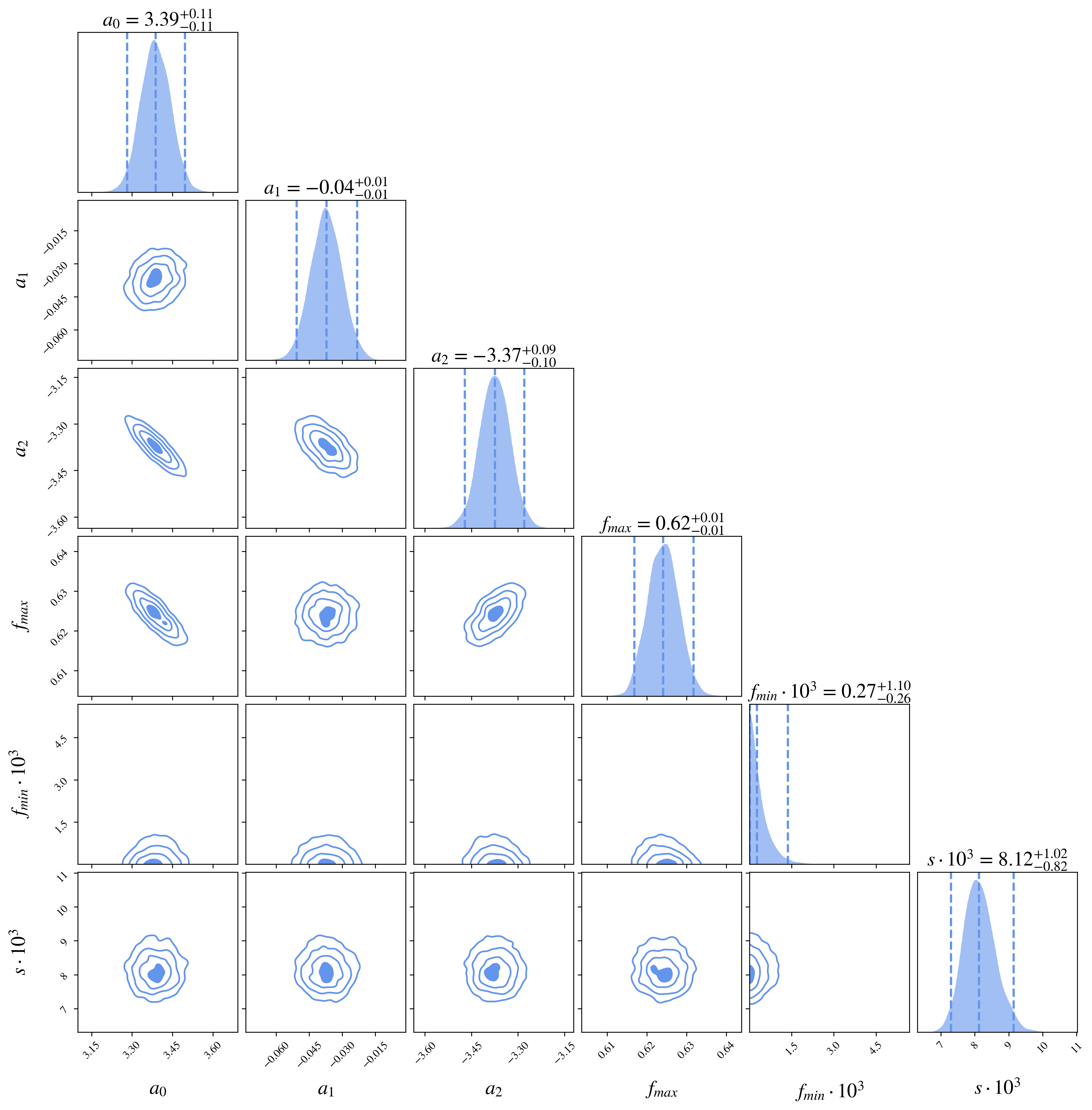
We assume broad uniform priors over all six parameters (), which are described in Appendix A. We sample from the posterior using dynesty (Speagle, 2020) v2.1.3 with the default settings, but impose a final dlogz threshold of to ensure denser sampling around the maximum likelihood solution. A corner plot summarizing the posterior and its uncertainties is shown in Appendix A, where our best-fit set of parameters, , can be input into Equation 1 to compute for any GC with a given and .
Based on our final set of posterior samples, we compute the posterior predictive for each by randomly resampling values from the final collection of samples. We compute the corresponding predictions for those values, and add in scatter to the predictions based on the associated value. The posterior predictive residuals shown in the right-hand panel of Figure 3 are computed using the median and the 16th/84th percentiles derived from this process.
In Figure 3, we also observe that the GC AM 4 exhibits the largest binary escape fraction, where of the binaries involved in three-body encounters producing single extra-tidal stars escape the cluster. AM 4 is also the cluster with the lowest escape velocity in the Baumgardt & Hilker (2018) catalogue. Conversely, the GC Liller 1 has the smallest escape binary fraction (and highest escape velocity), where only of three-body encounter binaries escape the cluster. In Figure 4, we compare the spatial and escape velocity distributions of the escaped binaries to the single extra-tidal stars of AM 4 and Liller 1. While escaped binaries of both clusters occupy a narrower distribution of orbital properties than escaped single stars, their properties are extremely comparable despite Liller 1 and AM 4 having the lowest and highest binary escape fractions.
3.3 Extra-tidal stars in different Galactic potential models
In addition to simulating the production and orbital evolution of extra-tidal stars and binaries in the baseline MWPotential2014 Galactic potential model, we also consider cases where host clusters and extra-tidal stars evolve in different potential models. As discussed in Section 2.3, we consider a model that also has a bar and transient spiral arms (Bar+Transient Wave potential), a model with a heavier halo (McMillan17), non-spherical halos, and a model that accounts for the presence of the LMC and its resulting perturbations to the Milky Way.

To observe how choice of Galactic potential model affects the kinematics of extra-tidal stars, we compare the action angle coordinates for extra-tidal stars between our static and time-dependent potentials. To span the complete action diamond, we examine actions for clusters located in different characteristic parts of the Galaxy. Specifically, we examine action coordinates in each potential for a disc cluster (NGC 104), a bulge cluster (NGC 104), an inner halo cluster (Palomar 5) and an outer halo cluster (Crater) in Figure 5.
Note that actions are always calculated in the baseline MWPotential2014 Galactic potential using the Stäckel approximation in galpy (Bovy, 2015), but the clusters have evolved in their own respective potentials. Hence, differences in the distributions of extra-tidal star actions are likely due to differences in the 6D-coordinates of the extra-tidal stars and not due to the assumed underlying potential. This approach is specifically necessary for models with time-dependent potentials as a calculation of extra-tidal star actions is not possible. This comparison is similar to assuming a potential like MWPotential2014 to calculate the actions of observed stars, even though they have evolved in the true potential of the Milky Way.
For each cluster, there are only minor differences in actions between the potentials, indicating that model of the Galactic potential has little influence on the actions of the extra-tidal stars. The general slight offsets in actions between the models could partially be attributed to artificial effects like the Stäckel approximation in galpy (Bovy, 2015). This occurs when a large gradient in the Galactic potential is present (e.g. in the inner regions of the Galaxy) and yields slightly different estimates of a cluster’s orbit depending on its orbital phase and the degree to which its orbit precesses every orbital period (see Appendix B for a full description of Stäckel effects). It is also possible that general interactions with various Galactic substructures could cause the orbits, and therefore orbit actions, of extra-tidal stars and their host GCs to change (Webb et al., 2020; Garrow et al., 2020).
The most prominent difference among models is for the GC Crater, where a slight bi-modality in the action distributions is enhanced. This could indeed be an artifact, given that Crater lies towards the edge of the action diamond. However action differences in this cluster are perhaps not unexpected, as the LMC would influence outer halo clusters the most.
Note that each of the above potentials assume a perfect dark matter halo sphericity (i.e. ). However, when varying levels of halo oblateness as described in Section 2.3.4, we once again find that the action distributions of the extra-tidal stars are comparable. This finding implies that the triaxiality of the Milky Way has little effect on the properties of extra-tidal stars produced by three-body encounters in GC cores, even for stars located far out in the Galactic halo (e.g. Crater).

3.4 The time (in)dependence of extra-tidal actions

While the specific rate of three-body encounters in a GC’s core depends on parameters like cluster core density and mass, extra-tidal stars will be ejected at random times throughout a GC’s orbit around the Galaxy. To investigate how cluster actions evolve as a function of time, we compare the present-day actions of each host GC to its actions based on its orbital coordinates five orbital periods in the past in Figure 6.
In time-independent potentials (e.g. MWPotential2014 and McMillan17), any evolution in cluster and extra-tidal actions is artificial and likely due to our use of the Stäckel approximation, as discussed in Appendix B. In most cases however, the shift is small, as and of clusters show shifts of less than 0.1 along both axes in the MWPotential2014 potential (left-most panel of Figure 6) and McMillan17 potential (third panel of Figure 6) respectively. If we compare the Corespray action distributions of the recent extra-tidal escapers to those that escaped early on in the MWPotential2014 Galactic potential model, we see that all but four clusters have the means of their distributions shift by less than 0.1. The four outliers – ESO 452-SC11, NGC 6380, NGC 6453 and NGC 6558 – all have kpc. It is therefore not surprising that the Stäckel approximation predicts different actions for the cluster as a function of time due to the gradient in the potential throughout this region, despite the potential being static.
In time-dependent potential models (e.g. Bar+Transient Wave Spiral and infall due to the LMC), a cluster’s actions will truly evolve due to interactions with substructure as opposed to the artificial evolution we see in the static potentials. In the Bar+Transient Wave potential (second panel of Figure 6), the change is still minimal with of clusters experiencing shifts in and less than 0.1 due to few clusters undergoing strong interactions with the Galactic disc. In fact, with most clusters orbiting in the halo, the presence of the LMC results in the largest evolution of cluster actions as only of clusters in this potential experience a shift along both axis less than 0.1 (right-most panel of Figure 6). Hence for most clusters, any evolution in action space due to time-dependent substructure is comparable to how a cluster’s calculated actions change with orbital phase when using the Stäckel approximation to calculate actions.
When comparing the GEMS catalogue to observations (e.g. when using Appendix D to associate field stars with individual GCs), it is important that actions are calculated in a self-consistent manner. If actions are calculated with the same method and in the same potential, the distributions given by Corespray simulations that use the baseline MWPotential2014 Galactic potential model can be used to search for extra-tidal stars that (i) are close to their host cluster and (ii) escaped recently. For extra-tidal stars that escaped long ago, the effects of spiral arms or the LMC should be considered depending on whether a low-latitude or outer region cluster is being studied.
4 Discussion
4.1 Core stars and binaries can contaminate stellar streams
4.1.1 The tidal tails of Palomar 13
Stellar streams are elongated distributions of escaped stars from GCs that are mainly believed to be the result of tidal stripping by the host Galaxy. In this scenario, mass segregation causes low mass stars in the GC to migrate to the outskirts, where tidal forces from the host galaxy gradually pull the stars away. Stars then escape through a cluster’s Lagrange points with velocities that are near-zero relative to the cluster itself. This process happens while the GC orbits the Galaxy, causing stars to form long, stretched out associations that lead and trail the cluster (e.g. Grillmair & Carlin, 2016, for an observational review of stellar streams in the Galactic halo).
As previously illustrated in Figure 1, extra-tidal star distributions for GCs with kpc in Baumgardt & Hilker (2018) can exhibit stream-like behaviour. We further investigate the structure of these distributions using an all-sky Mollweide projection in Figure 7. Here, it is evident that extra-tidal stars from halo GCs are primarily found in stellar streams, which are found all throughout the Milky Way. As discussed in Section 3.1.1, these stream-like properties often occur when a cluster has a low core escape velocity, such that three-body interactions that yield weak kicks result in the single star escaping the host cluster with a near-zero velocity relative to the cluster itself. Even though the kick is occurring in a random direction and the star isn’t necessarily escaping through the cluster’s Lagrange points like a tidally stripped star, the escaping star will still follow an orbit that is comparable to its progenitor cluster. Hence, the escaped stars populate streams that tail the cluster along its orbit of the Galaxy.
To explore this behaviour in more detail, in Figure 8 we plot the locations of extra-tidal tidal stars and binaries from the GC Palomar 13 – a cluster that was recently shown to have extended tidal tails 666See Piatti & Carballo-Bello (2020) for a complete list of GCs with observed tidal tails. (Shipp et al., 2020). From our Corespray simulation, it is immediately clear that both the single and binary extra-tidal stars of Palomar 13 exhibit stream-like behaviour. To further explore this statement, we compare our Palomar 13 Corespray stars to the Pal13-S20 stream in galstreams (Mateu, 2023) utilizing observed data from Shipp et al. (2020). From Figure 8, we see that the locations of the extra-tidal stars and binaries ejected from the core of Palomar 13 are consistent with the observed stellar stream stars. This overlap allows us to conclude that the tidal tails of Palomar 13 could be contaminated with stars and binaries from the cluster’s core. Importantly, this finding challenges the current belief that GC tidal tails or stellar streams are purely the result of tidal stripping, indicating that dynamical interactions such as three-body encounters could influence their overall composition.


Stellar streams are also believed to be kinematically “cold”, as stars escape a cluster with velocities close to the GC’s escape speed due to the constant pull of Galactic tidal forces. For three-body core encounters, however, the overall kick velocity distribution is governed by the core velocity dispersion of the cluster. The GC’s escape speed, on the other hand, just sets a boundary for what fraction of the kick distribution will actually escape. While core interactions yielding weak velocity kicks will result in stars escaping the host cluster with near-zero velocities relative to the cluster itself (comparable to tidal stripping), dynamical interactions can eject stars with a variety of velocities, often much higher than what would occur during tidal stripping. Thus, we also conclude it is possible that a stream contaminated by core stars and binaries could appear dynamically hotter and thicker than if it was just populated by tidally stripped stars. This finding has implications for methods that attempt to use stream properties to constrain the stream’s progenitor (Johnston, 1998; Webb & Bovy, 2019; Gialluca et al., 2021) or infer interactions with dark matter substructure (Bovy et al., 2017; Bonaca et al., 2019). For clusters with high three-body interaction rates, kicked core stars with stream-like orbits may also appear as diffuse stellar structure around the stream, similar to the observed cocoon around GD-1 (Malhan et al., 2019).
4.1.2 Stream contamination fractions from three-body encounters
While direct -body simulations with realistic binary fractions would be required to estimate the exact amount of contamination and the degree to which core stars might make a stream appear dynamically hotter, we can estimate the fraction of core stars from three-body encounters that contribute to the cluster mass loss rate due to tidal stripping. Equation 3 represents the total mass loss rate of the cluster (, where is the cluster mass from Baumgardt & Hilker (2018) and is the remaining cluster lifetime from Baumgardt & Makino (2003). Importantly, we treat this total mass loss rate to be approximately representative of the mass loss rate due to tidal stripping, since this is the dominant mass loss channel of evolved clusters in the present-day (e.g. Heggie & Hut, 2003).
| (3) |
The three-body interaction rate due to GC core three-body encounters is computed via Equation A10 in Leigh & Sills (2011), where is the binary fraction, is the triple fraction, is the core radius, is the mean stellar density in the core (computed from , and via Equation 13 in Leigh & Sills, 2011), is the velocity dispersion, is the mean stellar mass and is the semi-major axis of the binary. Note that to get a mass loss rate (), we assume an 100% stellar escape fraction and an average stellar escaper mass of and divide this by Equation 13 in Leigh & Sills (2011), yielding Equation 4.
| (4) |
To solve for , we adopt values of and , where we acknowledge that in reality, binary fraction decreases with cluster density (Milone et al., 2012). All GC structural parameters (e.g. , , and are taken from Baumgardt & Hilker, 2018). We also assume and , where corresponds to the hard-soft limit for binaries.
The mass loss fraction due to three-body encounters can be estimated by dividing Equation 4 by Equation 3, where . Figure 9 highlights for all GCs with kpc in our sample, as these are the clusters that typically exhibit stream-like behaviour in Figure 1. Clusters with tidal tails or extra-tidal features presented in Piatti & Carballo-Bello (2020) are highlighted in pink and green, respectively. Our case study cluster Palomar 13 is highlighted in yellow.
From Figure 9, it is clear that for many clusters, three-body encounters in GC cores can contribute a non-negligible amount to the mass loss rate due to tidal stripping. This holds true for Palomar 13, where we find that of the mass loss rate due to stripping could actually come from three-body encounters. Hence, it is indeed possible that a fraction of real stars in these streams could be extra-tidal single stars or binaries from the cluster cores.While such contamination would also make it more difficult to constrain a cluster’s dynamical history from variation in the mass function along the stream (Webb & Bovy, 2022), it may also provide further insight into the time evolution of a GC’s core.
It is of course important to note that is a simplified approximation. On one hand, not all three-body encounters will result in stellar escape from a cluster. However, mass segregation would imply that core stars are more likely to be brighter than most low-mass tidally stripped stars that have segregated to a cluster’s outer regions. Additionally, only a fraction of the stars that escaped via tidal stripping would be bright enough to observe given magnitude limits. Hence, the contamination fraction of observed core stars in stellar streams could be higher than our estimates here. A detailed quantitative follow-up of stellar stream contamination from GC core stars, binaries and even compact objects will be available in Grondin & Webb 2024, in preparation.
4.2 Identifying an extra-tidal star’s progenitor cluster
In order to quantify and illustrate how unique a given region of the action diamond parameter space is to extra-tidal stars from a single GC, we first estimate the probability distribution function , of each cluster’s mock extra-tidal stars. A Gaussian kernel density estimate of each distribution is determined from the extra-tidal mock stars 777See the gaussian_kde function in the scipy Python package (Virtanen et al., 2020)., after which the probability distribution function of each cluster is evaluated for a grid of points that spans the action diamond. At each location within the action diamond, we evaluate for each cluster and determine the cluster that yields the maximum . Furthermore, for the cluster with the highest evaluation of at a given location, we also calculate the logarithm of the odds ratio between that cluster and each of the other clusters in our dataset . Hence, the relative probability that an extra-tidal star with a given set of actions escaped from one GC to another can be determined, where the cluster with the highest probability will represent the extra-tidal star’s most likely origin.
Figure 10 illustrates four maps of the action diamond parameter space, colour coded by the cluster that yields at a given location. Outlines are drawn to highlight connected regions where the and values of mock extra-tidal stars indicate the stars are likely to share a common origin. In the top-left panel of Figure 10, each location is mapped to the cluster that yields the highest evaluation of regardless of how this cluster’s probability distribution compares to other clusters. We also require that at least 500 Corespray stars from the cluster that yield fall within a given data point to include it in Figure 10. Therefore, while this panel clearly demonstrates how the action diamond space can be broken up into regions that are more strongly associated with a given cluster, it does not take into consideration the fact that the distribution functions of other clusters might yield similar estimates of .
To identify regions of the action diamond parameter space where an extra-tidal star’s most likely origin is significantly more probable than any other cluster, we focus on regions where satisfies specific criteria. The maps in the top-right, bottom-left, and bottom-right panels of Figure 10 are again colour coded by the cluster that yields at a given location, but only show cases where is greater than 0.5, 1, and 2 respectively. These thresholds correspond to cases where the estimate of an extral-tidal star’s most likely origin are significant, strong, and decisive, using the Kass & Raftery (1995) metric. If we first consider the top-right panel of Figure 10, all whitespace can be considered as regions where the mock extra tidal star distributions of at least two clusters overlaps too much to strongly conclude that a star at the location in the action diamond is from one specific cluster. Regions that retain their colour coding demonstrate locations where an estimate of an extra-tidal star’s origin would be significant.
Taking into consideration the bottom two panels in Figure 10, we see that the parameter space over which one can strongly or decisively state that an extra-tidal star comes from a specific cluster becomes smaller and smaller compared to the case. However, there remain 21 clusters that occupy truly unique regions of the action diamond parameter space, such that a star observed in that region would most likely come from that cluster compared to any other. The 21 clusters labeled in the bottom-right corner of Figure 10 represent the most ideal GC candidates for kinematically searching for extra tidal stars. Appendix D outlines a Python code that (i) identifies the individual GC with the highest probability of association and (ii) computes the logarithm of the odds ratio between the first and second most likely progenitor clusters for any field star or binary.
It is important to note that these probability distribution functions do not represent the probability that a star was ejected from a given GC. Such a probability cannot be known without knowledge (or an estimate of) the dissolved star cluster population of the Milky Way and the orbital distribution of field stars in a given region. However, as described in Section 1, quantitatively associating stars with progenitor clusters is often done by incorporating chemistry along with dynamics (‘chemo-dynamical tagging’). If the chemical properties of an observed field star are also comparable to those of a GC that yields a large value of , it is stronger evidence that the field star was once located in the candidate cluster. A full Milky Way scale association of field stars to progenitor GCs could thus be achieved by applying the methods in Grondin et al. (2023) to clusters in the GEMS catalogue that have chemical data, for example.
The GEMS catalogue also allows for a more rigorous estimate of than presented in Figure 10. Calculating the probability distribution function from a four-dimensional Gaussian kernel density estimate of extra-tidal star distributions in , , , and orbital energy space would lift some of the degeneracies that exist in the action diamond parameter space. These four dimensions have been used to link Galactic GCs to specific accretion events in the Milky Way’s history (Myeong et al., 2019). The probability of association could also be improved by incorporating the expected number of ejected stars from each cluster given their current mass loss rates, or an evolutionary track, into the calculation.

5 Conclusions and Implications
In this study, we present the GEMS (Globular cluster Extra-tidal Mock Star) catalogue; a collection of simulated extra-tidal stars and binaries created from three-body encounters in GC cores. Extra-tidal stars and binaries of all 159 GCs listed in Baumgardt & Hilker (2018) are simulated using the Corespray software (Grondin et al., 2023), with stellar orbits integrated in seven different Galactic potential models. The main results and implications are summarized below.
-
1.
Extra-tidal stars and binaries of individual GCs generally occupy unique regions in both (i) location in the Galaxy (Figure 1) and (ii) the action diamond (Figure 2). Field stars and binaries can be matched with possible progenitor GCs using the kinematics presented in the GEMS catalogue (Section 4.2). Coupled with additional chemo-dynamical information, this tool can provide associations with corresponding probabilities of any given field star being associated with any Galactic GC. Furthermore, there are 21 clusters that occupy extremely unique regions of the action diamond (Figure 10), allowing for decisive associations of field stars with these clusters via the Kass & Raftery (1995) metric (Appendix D).
-
2.
We present a modified logistic function model for the escaped recoil binary fraction of any Galactic GC as a function of core density and cluster escape velocity in Equation 1. The best-fit model parameters are determined from the posterior predicative values calculated with the dynesty (Speagle, 2020) nested sampling code.
-
3.
Extra-tidal star characteristics are largely independent of the choice of Galactic potential model, where large-scale disc structure, perturbations from the LMC and mass and sphericity of the dark matter halo all appear to mostly be negligible (Section 3.3 and Figure 5). For the distributions of our Corespray simulated extra-tidal stars, slight differences in action coordinates are found between recent and old escapers for inner region clusters with kpc. However, this may be due to our use of the Stäckel approximation when calculating actions (Section 3.4 and Appendix B).
-
4.
Extra-tidal stars and binaries produced from three-body encounters in GC cores could contaminate stellar streams (Section 4.1, Figures 8 and 9). Contamination from core stars that escape with relative velocities higher than tidally stripped stars may cause streams to appear hotter. Since it is mainly believed that GC stellar streams are the products of tidal stripping (and thus contain low-mass stars), this novel result unveils possibilities for constraining stream progenitors or even explaining diffuse structure around observed streams (e.g. the observed cocoon around GD-1).
5.1 Future work
The GEMS catalogue provides a large sample of extra-tidal stars and binaries that can be used to probe cluster dynamics and evolution at a population-level scale. A few immediate applications of this catalogue and Corespray are listed below:
-
1.
The rate at which three-body interactions occur is highly dependent on the number, core density and velocity of stars in the core of the cluster itself (Binney & Tremaine, 2008) and the properties of its binary star population (Leigh & Sills, 2011). Taking these factors into consideration, one could use Corespray or sample the GEMS catalogue to generate realistic realizations of extra-tidal star distributions based on the expected number of extra-tidal stars ejected from each GC to determine the best GCs to observationally find extra-tidal stars. These identified stars could then be matched to individual GCs using the framework presented in Section 4.2 and Appendix D.
-
2.
In this study, we find that the spatial and action coordinate distributions of extra-tidal stars and binaries generally broaden as binaries escape at earlier times in the past. However, in clusters with high three-body interaction rates, one could use Corespray to probe cluster binary fraction as a function of time. This approach would allow for insights into the fraction of binaries that exist in a cluster at a given time, providing useful constraints for compact object interactions and high-velocity star production in the cores of GCs. Such an approach would also have to factor in the evolution of the binary populations binding energy distribution as well (Leigh et al., 2022).
Ultimately, combining extra-tidal star data from the GEMS catalogue with additional chemo-dynamical information (e.g. from APOGEE and Gaia) will allow field stars to be associated with individual Galactic GCs. As more extra-tidal stars are associated with clusters, we can continue to better our understanding of GC dynamics and evolution and begin to tackle big open questions like cluster formation too.
Acknowledgements
The authors thank Jo Bovy, Jason Hunt and Ting Li who provided important context, insight and references for the various Galactic potential models used in this study. The authors also acknowledge Fraser Evans and Phil Van-Lane for providing thorough feedback on the manuscript itself. Advice from Samantha Berek, Victor Chan, Maria Drout, Mairead Heiger, Marten van Kerkwijk and Claire Ye also greatly improved this work. SMG acknowledges the support of the Natural Sciences and Engineering Research Council of Canada (NSERC) and is partially funded through a NSERC Postgraduate Scholarship – Doctoral. SMG also recognizes current funding from a Walter C. Sumner Memorial Fellowship and an Ontario Graduate Scholarship (2022-2023). SMG wishes to thank Debbie, Dianne and Tom Postnikoff for meaningful support and atvar during the preparation of this manuscript. JJW acknowledges financial support from NSERC (funding reference number RGPIN-2020-04712) and an Ontario Early Researcher Award (ER16-12-061). JSS would like to acknowledge support from the Natural Sciences and Engineering Research Council of Canada (NSERC) funding reference #RGPIN-2023-04849. The Dunlap Institute is funded through an endowment established by the David Dunlap family and the University of Toronto. NWCL gratefully acknowledges the generous support of a Fondecyt Regular grant 1230082, as well as support from Millenium Nucleus NCN19_058 (TITANs) and funding via the BASAL Centro de Excelencia en Astrofisica y Tecnologias Afines (CATA) grant PFB-06/2007. NWCL also thanks support from ANID BASAL project ACE210002 and ANID BASAL projects ACE210002 and FB210003.
Data Availability
The GEMS catalogue is available online and can be downloaded at https://zenodo.org/record/8436703. There are two corresponding csv files containing data for (i) single extra-tidal stars and (ii) escaped recoil binaries, where orbits are integrated in our baseline MWPotential2014 potential. A description of each column is provided in a supplementary README.txt file. All individual GC structural parameters of M3 are obtained from Baumgardt & Hilker (2018), where the online database is accessible at https://people.smp.uq.edu.au/HolgerBaumgardt/globular/. The Corespray Python package can be downloaded at https://github.com/webbjj/corespray. The dynesty Python package (Speagle, 2020) is used to provide a functional form between escaped binary fraction, core density and escape velocity. This work also utilizes the astropy (Astropy Collaboration et al., 2022), numpy (Harris et al., 2020), scipy (Virtanen et al., 2020) and matplotlib (Hunter, 2007) Python packages.
References
- Aarseth (2003) Aarseth S. J., 2003, Gravitational N-Body Simulations
- Abadi et al. (2010) Abadi M. G., Navarro J. F., Fardal M., Babul A., Steinmetz M., 2010, MNRAS, 407, 435
- Abdurro’uf et al. (2022) Abdurro’uf et al., 2022, ApJS, 259, 35
- Alexander & Gieles (2012) Alexander P. E. R., Gieles M., 2012, MNRAS, 422, 3415
- Astropy Collaboration et al. (2022) Astropy Collaboration et al., 2022, apj, 935, 167
- Banik & Bovy (2019) Banik N., Bovy J., 2019, MNRAS, 484, 2009
- Baumgardt & Hilker (2018) Baumgardt H., Hilker M., 2018, MNRAS, 478, 1520
- Baumgardt & Makino (2003) Baumgardt H., Makino J., 2003, MNRAS, 340, 227
- Baumgardt & Vasiliev (2021) Baumgardt H., Vasiliev E., 2021, MNRAS, 505, 5957
- Baumgardt et al. (2019) Baumgardt H., Hilker M., Sollima A., Bellini A., 2019, MNRAS, 482, 5138
- Binney (2012) Binney J., 2012, MNRAS, 426, 1324
- Binney & Tremaine (2008) Binney J., Tremaine S., 2008, Galactic Dynamics: Second Edition
- Bird et al. (2022) Bird S. A., et al., 2022, MNRAS, 516, 731
- Bland-Hawthorn & Gerhard (2016) Bland-Hawthorn J., Gerhard O., 2016, ARA&A, 54, 529
- Blitz & Spergel (1991) Blitz L., Spergel D. N., 1991, ApJ, 379, 631
- Bonaca et al. (2019) Bonaca A., Hogg D. W., Price-Whelan A. M., Conroy C., 2019, ApJ, 880, 38
- Bovy (2015) Bovy J., 2015, ApJS, 216, 29
- Bovy & Rix (2013) Bovy J., Rix H.-W., 2013, ApJ, 779, 115
- Bovy et al. (2017) Bovy J., Erkal D., Sanders J. L., 2017, MNRAS, 466, 628
- Cabrera & Rodriguez (2023) Cabrera T., Rodriguez C. L., 2023, ApJ, 953, 19
- Casamiquela et al. (2021) Casamiquela L., Castro-Ginard A., Anders F., Soubiran C., 2021, A&A, 654, A151
- Castro-Ginard et al. (2021) Castro-Ginard A., et al., 2021, A&A, 652, A162
- Chen et al. (2018) Chen B., D’Onghia E., Pardy S. A., Pasquali A., Bertelli Motta C., Hanlon B., Grebel E. K., 2018, ApJ, 860, 70
- Chun et al. (2020) Chun S.-H., Lee J.-J., Lim D., 2020, ApJ, 900, 146
- Conroy et al. (2021) Conroy C., Naidu R. P., Garavito-Camargo N., Besla G., Zaritsky D., Bonaca A., Johnson B. D., 2021, Nature, 592, 534
- Deason et al. (2021) Deason A. J., et al., 2021, MNRAS, 501, 5964
- Dehnen (2000) Dehnen W., 2000, AJ, 119, 800
- Dubinski (1994) Dubinski J., 1994, ApJ, 431, 617
- Eadie & Jurić (2019) Eadie G., Jurić M., 2019, ApJ, 875, 159
- Eilers et al. (2019) Eilers A.-C., Hogg D. W., Rix H.-W., Ness M. K., 2019, ApJ, 871, 120
- Erkal et al. (2021) Erkal D., et al., 2021, MNRAS, 506, 2677
- Ferrone et al. (2023) Ferrone S., Di Matteo P., Mastrobuono-Battisti A., Haywood M., Snaith O. N., Montuori M., Khoperskov S., Valls-Gabaud D., 2023, A&A, 673, A44
- Forbes & Bridges (2010) Forbes D. A., Bridges T., 2010, MNRAS, 404, 1203
- Gaia Collaboration et al. (2016) Gaia Collaboration et al., 2016, A&A, 595, A1
- Gaia Collaboration et al. (2018) Gaia Collaboration et al., 2018, A&A, 616, A12
- Garavito-Camargo et al. (2019) Garavito-Camargo N., Besla G., Laporte C. F. P., Johnston K. V., Gómez F. A., Watkins L. L., 2019, ApJ, 884, 51
- Garavito-Camargo et al. (2021) Garavito-Camargo N., Besla G., Laporte C. F. P., Price-Whelan A. M., Cunningham E. C., Johnston K. V., Weinberg M., Gómez F. A., 2021, ApJ, 919, 109
- Garrow et al. (2020) Garrow T., Webb J. J., Bovy J., 2020, MNRAS, 499, 804
- Gialluca et al. (2021) Gialluca M. T., Naidu R. P., Bonaca A., 2021, ApJ, 911, L32
- Grillmair & Carlin (2016) Grillmair C. J., Carlin J. L., 2016, in Newberg H. J., Carlin J. L., eds, Astrophysics and Space Science Library Vol. 420, Tidal Streams in the Local Group and Beyond. p. 87 (arXiv:1603.08936), doi:10.1007/978-3-319-19336-6˙4
- Grondin et al. (2023) Grondin S. M., Webb J. J., Leigh N. W. C., Speagle J. S., Khalifeh R. J., 2023, MNRAS, 518, 4249
- Hanke et al. (2020) Hanke M., Koch A., Prudil Z., Grebel E. K., Bastian U., 2020, A&A, 637, A98
- Harfst et al. (2007) Harfst S., Gualandris A., Merritt D., Spurzem R., Portegies Zwart S., Berczik P., 2007, New Astron., 12, 357
- Harris (1996) Harris W. E., 1996, AJ, 112, 1487
- Harris et al. (2020) Harris C. R., et al., 2020, Nature, 585, 357
- Hattori et al. (2016) Hattori K., Erkal D., Sanders J. L., 2016, MNRAS, 460, 497
- Heggie (2014) Heggie D. C., 2014, MNRAS, 445, 3435
- Heggie & Hut (2003) Heggie D., Hut P., 2003, The Gravitational Million-Body Problem: A Multidisciplinary Approach to Star Cluster Dynamics
- Hunt et al. (2019) Hunt J. A. S., Bub M. W., Bovy J., Mackereth J. T., Trick W. H., Kawata D., 2019, MNRAS, 490, 1026
- Hunter (2007) Hunter J. D., 2007, Computing in Science & Engineering, 9, 90
- Irrgang et al. (2013) Irrgang A., Wilcox B., Tucker E., Schiefelbein L., 2013, A&A, 549, A137
- Johnston (1998) Johnston K. V., 1998, ApJ, 495, 297
- Kass & Raftery (1995) Kass R., Raftery A., 1995, Journal of the American Statistical Association, 90, 773
- Kazantzidis et al. (2010) Kazantzidis S., Abadi M. G., Navarro J. F., 2010, ApJ, 720, L62
- Koposov et al. (2010) Koposov S. E., Rix H.-W., Hogg D. W., 2010, ApJ, 712, 260
- Kos et al. (2018) Kos J., et al., 2018, MNRAS, 473, 4612
- Kroupa (2001) Kroupa P., 2001, MNRAS, 322, 231
- Küpper et al. (2011) Küpper A. H. W., Maschberger T., Kroupa P., Baumgardt H., 2011, MNRAS, 417, 2300
- Lane et al. (2022) Lane J. M. M., Bovy J., Mackereth J. T., 2022, MNRAS, 510, 5119
- Leigh & Sills (2011) Leigh N., Sills A., 2011, MNRAS, 410, 2370
- Leigh et al. (2022) Leigh N. W. C., Stone N. C., Webb J. J., Lyra W., 2022, MNRAS, 517, 3838
- Leigh et al. (2023) Leigh N. W. C., Ye C. S., Grondin S. M., Fragione G., Webb J. J., Heinke C. O., 2023, arXiv e-prints, p. arXiv:2309.13122
- Mackereth & Bovy (2018) Mackereth J. T., Bovy J., 2018, PASP, 130, 114501
- Malhan & Ibata (2019) Malhan K., Ibata R. A., 2019, MNRAS, 486, 2995
- Malhan et al. (2019) Malhan K., Ibata R. A., Carlberg R. G., Valluri M., Freese K., 2019, ApJ, 881, 106
- Masseron et al. (2019) Masseron T., et al., 2019, A&A, 622, A191
- Mateu (2023) Mateu C., 2023, MNRAS, 520, 5225
- McInnes et al. (2018) McInnes L., Healy J., Melville J., 2018, arXiv e-prints, p. arXiv:1802.03426
- McLaughlin et al. (2008) McLaughlin D. E., Barmby P., Harris W. E., Forbes D. A., Harris G. L. H., 2008, MNRAS, 384, 563
- McMillan (2017) McMillan P. J., 2017, MNRAS, 465, 76
- Mészáros et al. (2020) Mészáros S., et al., 2020, MNRAS, 492, 1641
- Milone et al. (2012) Milone A. P., et al., 2012, A&A, 540, A16
- Miyamoto & Nagai (1975) Miyamoto M., Nagai R., 1975, PASJ, 27, 533
- Myeong et al. (2019) Myeong G. C., Vasiliev E., Iorio G., Evans N. W., Belokurov V., 2019, MNRAS, 488, 1235
- Navarro et al. (1996) Navarro J. F., Frenk C. S., White S. D. M., 1996, ApJ, 462, 563
- Ness et al. (2018) Ness M., et al., 2018, ApJ, 853, 198
- Ness et al. (2019) Ness M. K., Johnston K. V., Blancato K., Rix H. W., Beane A., Bird J. C., Hawkins K., 2019, ApJ, 883, 177
- Palau & Miralda-Escudé (2023) Palau C. G., Miralda-Escudé J., 2023, MNRAS,
- Pearson et al. (2017) Pearson S., Price-Whelan A. M., Johnston K. V., 2017, Nature Astronomy, 1, 633
- Piatti & Carballo-Bello (2020) Piatti A. E., Carballo-Bello J. A., 2020, A&A, 637, L2
- Posti & Helmi (2019) Posti L., Helmi A., 2019, A&A, 621, A56
- Price-Jones et al. (2020) Price-Jones N., et al., 2020, MNRAS, 496, 5101
- Price-Whelan et al. (2016) Price-Whelan A. M., Sesar B., Johnston K. V., Rix H.-W., 2016, ApJ, 824, 104
- Rodriguez et al. (2022) Rodriguez C. L., et al., 2022, ApJS, 258, 22
- Sanders (2012) Sanders J., 2012, MNRAS, 426, 128
- Schiavon et al. (2017) Schiavon R. P., et al., 2017, MNRAS, 466, 1010
- Shipp et al. (2020) Shipp N., Price-Whelan A. M., Tavangar K., Mateu C., Drlica-Wagner A., 2020, AJ, 160, 244
- Shu (2016) Shu F. H., 2016, ARA&A, 54, 667
- Speagle (2020) Speagle J. S., 2020, MNRAS, 493, 3132
- Thomas et al. (2023) Thomas G. F., Famaey B., Monari G., Laporte C. F. P., Ibata R., de Laverny P., Hill V., Boily C., 2023, arXiv e-prints, p. arXiv:2309.05733
- Valtonen & Karttunen (2006) Valtonen M., Karttunen H., 2006, Cambridge University Press
- Van der Maaten & Hinton (2008) Van der Maaten L., Hinton G., 2008, Journal of Machine Learning Research, 9, 2579
- Vasiliev (2019) Vasiliev E., 2019, MNRAS, 484, 2832
- Vasiliev (2023) Vasiliev E., 2023, Galaxies, 11
- Vasiliev & Baumgardt (2021) Vasiliev E., Baumgardt H., 2021, MNRAS, 505, 5978
- Vera-Ciro & Helmi (2013) Vera-Ciro C., Helmi A., 2013, ApJ, 773, L4
- Virtanen et al. (2020) Virtanen P., et al., 2020, Nature Methods, 17, 261
- Wang et al. (2016) Wang L., et al., 2016, MNRAS, 458, 1450
- Wang et al. (2020) Wang L., Iwasawa M., Nitadori K., Makino J., 2020, MNRAS, 497, 536
- Weatherford et al. (2023) Weatherford N. C., Kıroğlu F., Fragione G., Chatterjee S., Kremer K., Rasio F. A., 2023, ApJ, 946, 104
- Webb & Bovy (2019) Webb J. J., Bovy J., 2019, MNRAS, 485, 5929
- Webb & Bovy (2022) Webb J. J., Bovy J., 2022, MNRAS, 510, 774
- Webb et al. (2013) Webb J. J., Harris W. E., Sills A., Hurley J. R., 2013, ApJ, 764, 124
- Webb et al. (2020) Webb J. J., Price-Jones N., Bovy J., Portegies Zwart S., Hunt J. A. S., Mackereth J. T., Leung H. W., 2020, MNRAS, 494, 2268
- Webb et al. (2022) Webb J., Starkman N., Bovy J., 2022, webbjj/clustertools: clustertools v1.0, doi:10.5281/zenodo.6656647, https://doi.org/10.5281/zenodo.6656647
Appendix A Logistic escaped binary fraction model parameter estimation
From Figure 3, we observe a correlation between , , and escaped binary fraction (). As discussed in Section 3.2, we model as a function of and with a modified logistic function (Equation 1). We fit for five free parameters in Equation 1: , where we originally assume broad uniform priors and determine the best fit parameters by sampling from the posterior using dynesty (Speagle, 2020) v2.1.3. Figure 11 shows a cornerplot that summarizes the posterior distributions (and uncertainties) for each of the free parameters.
Appendix B Stäckel approximation effects
As discussed in Sections 3.1.2 and 3.3, actions in this study are computed using the Stäckel approximation in galpy (Bovy, 2015). In a static potential, actions are a conserved quantity. However, in Figure 6 we see that the actions of individual GCs in the baseline MWPotential2014 Galactic potential model have different actions at the beginning and end of the simulation. The clusters that exhibit the largest change in actions are those with small pericentre radii. The use of the Stäckel approximation in regions where the gradient in the Galactic potential is large, like the inner regions of the Galaxy, can lead to slightly different estimates of a cluster’s orbit depending on its orbital phase and the degree to which its orbit precesses every orbital period. Hence, this shift is artificial and simply the result of our method for calculating actions.
To show this shift in actions as a function of pericentric radius, we compare the mean action coordinates of recent escapers to early escapers for our Corespray extra-tidal star distributions. For clusters with Gyr, we compare stars that escaped within one to those that escaped between four and five orbital periods in the past. For the 14 clusters listed in Section 2.2.1 with Gyr, we compare the most recently escaped 10,000 Corespray extra-tidal stars to the mean action coordinates of the first 10,000 escapers. In Figure 12, it is evident that there is a general trend of increasing shifts in action for decreasing pericentre radii. Clusters with pericentric radii smaller than five kiloparsecs typically exhibit the largest shifts in actions between recent and old escapers. Hence, these shifts are an artificial effect with inner clusters being more significant affected.

Appendix C Action Coordinate Parameters
To roughly determine a host cluster association for a given extra-tidal star in the field, we list the action coordinates for each GC and the associated GEMS distribution in Table LABEL:tab:actiontable. Specifically, we present Jϕ / Jtot and (JJR)/ Jtot for each GC analyzed in this study, with action coordinates computed using the orbital parameters in Baumgardt & Hilker (2018) and the Stäckel approximation in galpy (Bovy, 2015). The mean ¡Jϕ / Jtot¿ and ¡(JJR)/ Jtot¿ values and corresponding standard deviations for the extra-tidal distributions are computed similarly (see Section 3.1.2 for details).
| Globular Cluster | Jϕ / Jtot (GC) | (JJR)/ Jtot (GC) | ¡Jϕ / Jtot¿ (ET stars) | ¡(JJR)/ Jtot¿ (ET stars) |
|---|---|---|---|---|
| 2MASS-GC01 | 0.98 | -0.018 | 0.955 0.067 | -0.034 0.056 |
| 2MASS-GC02 | 0.289 | -0.504 | 0.269 0.162 | -0.453 0.164 |
| AM_1 | -0.103 | -0.703 | -0.093 0.148 | -0.583 0.255 |
| AM_4 | -0.28 | 0.611 | -0.273 0.075 | 0.587 0.128 |
| Arp_2 | 0.157 | 0.209 | 0.149 0.124 | 0.182 0.222 |
| BH_140 | 0.026 | -0.972 | 0.015 0.229 | -0.707 0.347 |
| BH_261 | 0.765 | 0.078 | 0.742 0.096 | 0.057 0.086 |
| Crater | -0.141 | 0.658 | -0.135 0.098 | 0.596 0.232 |
| Djor_1 | 0.394 | -0.575 | 0.366 0.193 | -0.539 0.183 |
| Djor_2 | -0.751 | 0.04 | -0.714 0.132 | 0.035 0.111 |
| ESO_280-SC06 | 0.284 | -0.269 | 0.269 0.125 | -0.263 0.153 |
| ESO_452-SC11 | 0.036 | 0.4 | 0.034 0.124 | 0.338 0.184 |
| E_3 | 0.833 | 0.073 | 0.814 0.074 | 0.064 0.073 |
| Eridanus | 0.067 | -0.097 | 0.063 0.123 | -0.099 0.234 |
| FSR_1716 | 0.828 | -0.003 | 0.802 0.092 | -0.012 0.084 |
| FSR_1735 | 0.613 | -0.163 | 0.579 0.152 | -0.13 0.146 |
| FSR_1758 | -0.568 | -0.227 | -0.529 0.169 | -0.212 0.181 |
| HP_1 | 0.076 | -0.913 | 0.065 0.25 | -0.633 0.324 |
| IC_1257 | -0.118 | -0.743 | -0.107 0.179 | -0.66 0.216 |
| IC_1276 | 0.899 | -0.072 | 0.869 0.092 | -0.086 0.081 |
| IC_4499 | -0.289 | 0.099 | -0.272 0.137 | 0.084 0.211 |
| Laevens_3 | 0.258 | -0.092 | 0.247 0.111 | -0.087 0.179 |
| Liller_1 | -0.411 | -0.552 | -0.246 0.438 | -0.305 0.301 |
| Lynga_7 | 0.786 | -0.065 | 0.758 0.11 | -0.074 0.096 |
| NGC_104 | 0.843 | 0.142 | 0.771 0.123 | 0.097 0.125 |
| NGC_1261 | -0.202 | -0.392 | -0.174 0.191 | -0.305 0.259 |
| NGC_1851 | -0.109 | -0.628 | -0.08 0.279 | -0.373 0.315 |
| NGC_1904 | -0.019 | -0.775 | -0.015 0.242 | -0.553 0.287 |
| NGC_2298 | -0.236 | -0.479 | -0.211 0.189 | -0.41 0.225 |
| NGC_2419 | 0.313 | -0.137 | 0.276 0.19 | -0.114 0.28 |
| NGC_2808 | 0.21 | -0.735 | 0.16 0.326 | -0.503 0.306 |
| NGC_288 | -0.331 | 0.05 | -0.31 0.128 | 0.047 0.174 |
| NGC_3201 | -0.603 | -0.26 | -0.554 0.181 | -0.238 0.188 |
| NGC_362 | -0.023 | -0.339 | -0.018 0.189 | -0.174 0.274 |
| NGC_4147 | -0.016 | -0.395 | -0.014 0.129 | -0.288 0.253 |
| NGC_4372 | 0.809 | -0.044 | 0.774 0.11 | -0.059 0.101 |
| NGC_4590 | 0.509 | -0.13 | 0.473 0.159 | -0.122 0.191 |
| NGC_4833 | 0.289 | -0.632 | 0.257 0.221 | -0.568 0.2 |
| NGC_5024 | 0.202 | 0.546 | 0.187 0.14 | 0.476 0.228 |
| NGC_5053 | 0.211 | 0.741 | 0.204 0.094 | 0.697 0.143 |
| NGC_5139 | -0.609 | -0.103 | -0.525 0.227 | -0.119 0.223 |
| NGC_5272 | 0.395 | 0.211 | 0.359 0.157 | 0.186 0.222 |
| NGC_5286 | -0.249 | -0.567 | -0.203 0.273 | -0.423 0.29 |
| NGC_5466 | -0.131 | -0.238 | -0.122 0.139 | -0.213 0.238 |
| NGC_5634 | 0.208 | -0.021 | 0.186 0.161 | -0.005 0.259 |
| NGC_5694 | -0.14 | -0.656 | -0.106 0.257 | -0.338 0.343 |
| NGC_5824 | 0.48 | 0.251 | 0.413 0.188 | 0.178 0.27 |
| NGC_5897 | 0.351 | 0.253 | 0.331 0.117 | 0.235 0.167 |
| NGC_5904 | 0.104 | -0.296 | 0.087 0.198 | -0.211 0.315 |
| NGC_5927 | 0.957 | 0.003 | 0.916 0.086 | -0.019 0.075 |
| NGC_5946 | 0.085 | -0.505 | 0.071 0.22 | -0.421 0.231 |
| NGC_5986 | 0.28 | -0.111 | 0.242 0.201 | -0.125 0.222 |
| NGC_6093 | 0.166 | 0.679 | 0.139 0.143 | 0.495 0.237 |
| NGC_6101 | -0.492 | -0.257 | -0.455 0.168 | -0.229 0.196 |
| NGC_6121 | 0.369 | -0.619 | 0.322 0.239 | -0.496 0.259 |
| NGC_6139 | 0.509 | 0.227 | 0.452 0.174 | 0.181 0.189 |
| NGC_6144 | -0.301 | 0.52 | -0.294 0.1 | 0.484 0.136 |
| NGC_6171 | 0.5 | 0.299 | 0.466 0.122 | 0.25 0.137 |
| NGC_6205 | -0.273 | 0.084 | -0.235 0.179 | 0.077 0.243 |
| NGC_6218 | 0.631 | 0.229 | 0.596 0.11 | 0.199 0.118 |
| NGC_6229 | 0.08 | -0.498 | 0.065 0.205 | -0.327 0.303 |
| NGC_6235 | 0.582 | 0.124 | 0.556 0.12 | 0.109 0.14 |
| NGC_6254 | 0.609 | 0.177 | 0.567 0.132 | 0.145 0.138 |
| NGC_6256 | 0.877 | 0.057 | 0.84 0.102 | 0.039 0.08 |
| NGC_6266 | 0.722 | 0.155 | 0.63 0.193 | 0.047 0.169 |
| NGC_6273 | -0.168 | 0.136 | -0.159 0.186 | 0.134 0.248 |
| NGC_6284 | -0.075 | -0.09 | -0.064 0.166 | -0.006 0.237 |
| NGC_6287 | 0.015 | 0.039 | 0.015 0.187 | -0.119 0.237 |
| NGC_6293 | -0.227 | 0.038 | -0.205 0.176 | 0.066 0.216 |
| NGC_6304 | 0.837 | 0.053 | 0.801 0.108 | 0.037 0.088 |
| NGC_6316 | 0.576 | -0.063 | 0.526 0.182 | -0.117 0.158 |
| NGC_6325 | -0.331 | 0.332 | -0.323 0.142 | 0.276 0.168 |
| NGC_6333 | 0.243 | -0.206 | 0.225 0.213 | -0.21 0.24 |
| NGC_6341 | 0.02 | -0.164 | 0.016 0.183 | -0.065 0.274 |
| NGC_6342 | 0.35 | 0.46 | 0.337 0.116 | 0.437 0.144 |
| NGC_6352 | 0.946 | 0.028 | 0.917 0.071 | 0.014 0.059 |
| NGC_6355 | -0.17 | 0.119 | -0.164 0.167 | 0.061 0.196 |
| NGC_6356 | 0.699 | 0.08 | 0.647 0.14 | 0.056 0.149 |
| NGC_6362 | 0.647 | 0.261 | 0.618 0.096 | 0.234 0.107 |
| NGC_6366 | 0.749 | -0.054 | 0.723 0.1 | -0.067 0.093 |
| NGC_6380 | -0.33 | -0.389 | -0.287 0.22 | -0.229 0.277 |
| NGC_6388 | -0.642 | -0.075 | -0.543 0.232 | -0.087 0.213 |
| NGC_6397 | 0.388 | -0.6 | 0.346 0.232 | -0.491 0.252 |
| NGC_6401 | -0.2 | -0.379 | -0.183 0.199 | -0.27 0.24 |
| NGC_6402 | 0.349 | 0.126 | 0.304 0.191 | 0.056 0.208 |
| NGC_6426 | 0.629 | -0.188 | 0.598 0.137 | -0.183 0.143 |
| NGC_6440 | -0.403 | 0.023 | -0.324 0.256 | 0.016 0.295 |
| NGC_6441 | 0.768 | -0.09 | 0.659 0.215 | -0.123 0.193 |
| NGC_6453 | 0.196 | 0.084 | 0.171 0.162 | 0.189 0.237 |
| NGC_6496 | 0.694 | 0.082 | 0.676 0.099 | 0.075 0.102 |
| NGC_6517 | 0.363 | -0.218 | 0.307 0.242 | -0.208 0.212 |
| NGC_6522 | 0.368 | 0.511 | 0.333 0.14 | 0.435 0.182 |
| NGC_6528 | 0.208 | -0.016 | 0.201 0.202 | -0.108 0.169 |
| NGC_6535 | -0.589 | -0.178 | -0.559 0.14 | -0.179 0.123 |
| NGC_6539 | 0.566 | 0.392 | 0.535 0.109 | 0.357 0.12 |
| NGC_6541 | 0.526 | 0.104 | 0.496 0.153 | 0.123 0.165 |
| NGC_6544 | 0.379 | -0.581 | 0.32 0.262 | -0.44 0.279 |
| NGC_6553 | 0.971 | -0.006 | 0.93 0.085 | -0.03 0.072 |
| NGC_6558 | 0.21 | 0.031 | 0.196 0.191 | -0.078 0.227 |
| NGC_6569 | 0.811 | 0.156 | 0.768 0.105 | 0.133 0.096 |
| NGC_6584 | 0.257 | -0.423 | 0.235 0.18 | -0.352 0.235 |
| NGC_6624 | 0.123 | 0.708 | 0.114 0.103 | 0.597 0.214 |
| NGC_6626 | 0.465 | -0.168 | 0.401 0.229 | -0.116 0.243 |
| NGC_6637 | 0.246 | 0.727 | 0.23 0.096 | 0.658 0.142 |
| NGC_6638 | 0.119 | -0.044 | 0.098 0.212 | -0.136 0.3 |
| NGC_6642 | -0.177 | -0.037 | -0.155 0.228 | -0.178 0.253 |
| NGC_6652 | 0.085 | 0.417 | 0.078 0.127 | 0.374 0.224 |
| NGC_6656 | 0.648 | -0.148 | 0.593 0.179 | -0.151 0.182 |
| NGC_6681 | -0.011 | -0.202 | -0.009 0.173 | 0.012 0.258 |
| NGC_6712 | -0.082 | -0.29 | -0.071 0.191 | -0.288 0.226 |
| NGC_6715 | 0.138 | 0.205 | 0.096 0.271 | 0.056 0.456 |
| NGC_6717 | 0.583 | 0.344 | 0.551 0.11 | 0.301 0.115 |
| NGC_6723 | 0.03 | 0.776 | 0.03 0.091 | 0.69 0.18 |
| NGC_6749 | 0.768 | -0.216 | 0.736 0.135 | -0.229 0.116 |
| NGC_6752 | 0.841 | 0.095 | 0.791 0.11 | 0.067 0.104 |
| NGC_6760 | 0.774 | -0.186 | 0.733 0.142 | -0.2 0.125 |
| NGC_6779 | -0.263 | -0.327 | -0.236 0.191 | -0.272 0.234 |
| NGC_6809 | 0.298 | 0.161 | 0.277 0.139 | 0.144 0.185 |
| NGC_6838 | 0.967 | -0.009 | 0.939 0.073 | -0.024 0.062 |
| NGC_6864 | 0.191 | -0.4 | 0.147 0.255 | -0.251 0.314 |
| NGC_6934 | 0.236 | -0.698 | 0.203 0.237 | -0.527 0.28 |
| NGC_6981 | 0.015 | -0.663 | 0.012 0.178 | -0.521 0.258 |
| NGC_7006 | -0.155 | -0.684 | -0.134 0.21 | -0.512 0.286 |
| NGC_7078 | 0.718 | 0.026 | 0.638 0.174 | -0.006 0.186 |
| NGC_7089 | -0.122 | -0.49 | -0.095 0.252 | -0.302 0.317 |
| NGC_7099 | -0.254 | 0.154 | -0.228 0.152 | 0.135 0.214 |
| NGC_7492 | -0.037 | -0.022 | -0.034 0.119 | -0.034 0.214 |
| Pal_10 | 0.907 | -0.08 | 0.865 0.111 | -0.096 0.098 |
| Pal_11 | 0.829 | 0.096 | 0.807 0.073 | 0.084 0.071 |
| Pal_12 | 0.234 | -0.022 | 0.223 0.12 | -0.025 0.193 |
| Pal_13 | -0.187 | -0.296 | -0.179 0.109 | -0.268 0.187 |
| Pal_14 | -0.016 | -0.895 | -0.014 0.15 | -0.724 0.267 |
| Pal_15 | 0.07 | -0.575 | 0.063 0.122 | -0.493 0.234 |
| Pal_1 | 0.95 | 0.025 | 0.928 0.071 | 0.015 0.061 |
| Pal_2 | 0.104 | -0.878 | 0.088 0.243 | -0.663 0.293 |
| Pal_3 | 0.236 | 0.625 | 0.223 0.105 | 0.564 0.227 |
| Pal_4 | -0.041 | -0.53 | -0.038 0.131 | -0.466 0.235 |
| Pal_5 | 0.381 | 0.549 | 0.372 0.078 | 0.527 0.109 |
| Pal_6 | -0.044 | -0.22 | -0.038 0.212 | -0.182 0.176 |
| Pal_8 | 0.675 | -0.042 | 0.643 0.119 | -0.046 0.11 |
| Pyxis | -0.081 | -0.039 | -0.074 0.12 | -0.049 0.247 |
| Rup_106 | 0.377 | -0.339 | 0.355 0.149 | -0.31 0.183 |
| Sagittarius_II | 0.412 | 0.144 | 0.39 0.121 | 0.119 0.2 |
| Ter_10 | 0.285 | -0.079 | 0.25 0.199 | -0.06 0.235 |
| Ter_12 | 0.828 | -0.039 | 0.794 0.112 | -0.052 0.095 |
| Ter_1 | 0.734 | -0.256 | 0.675 0.198 | -0.274 0.155 |
| Ter_2 | -0.71 | 0.101 | -0.647 0.177 | 0.076 0.155 |
| Ter_3 | 0.729 | 0.205 | 0.711 0.082 | 0.196 0.079 |
| Ter_4 | 0.589 | 0.19 | 0.528 0.187 | 0.13 0.19 |
| Ter_5 | 0.513 | -0.381 | 0.426 0.3 | -0.361 0.219 |
| Ter_6 | -0.647 | -0.157 | -0.562 0.247 | -0.17 0.189 |
| Ter_7 | 0.105 | 0.108 | 0.098 0.129 | 0.084 0.231 |
| Ter_8 | 0.107 | 0.092 | 0.1 0.131 | 0.07 0.245 |
| Ter_9 | 0.497 | -0.408 | 0.44 0.244 | -0.402 0.19 |
| Ton_2 | 0.706 | 0.095 | 0.678 0.108 | 0.084 0.107 |
| UKS_1 | 0.18 | -0.791 | 0.161 0.21 | -0.71 0.186 |
| VVV-CL001 | -0.559 | -0.378 | -0.519 0.2 | -0.367 0.165 |
| Whiting_1 | 0.173 | 0.33 | 0.167 0.099 | 0.305 0.184 |
Appendix D Associating Extra-Tidal Field Stars with Individual Globular Clusters
Using , and action coordinates from the GEMS catalogue, one can determine the probability that any given field star originated from a certain GC using the Python code presented below. Specifically, this code uses a Gaussian kernel density estimator to compute both (i) the most likely cluster that the extra-tidal star originated from and (ii) the logarithm of the odds ratio between the first and second most likely progenitor clusters. For consistency between data sets, it is important to compute action coordinates of field stars using the Stäckel approximation in galpy (Bovy, 2015).
