跳到论文正文
W Papers独立论文阅读器 arXiv:2310.01762 论文正文 计算阅读时间 · 0%
引用这篇论文根据当前论文元数据生成,正式投稿前建议核对。


Sampling Multimodal Distributions with the Vanilla Score: Benefits of Data-Based Initialization

Frederic Koehler Stanford University, {fkoehler,tdvuong}@stanford.edu Thuy-Duong Vuong Stanford University, {fkoehler,tdvuong}@stanford.edu
Abstract

There is a long history, as well as a recent explosion of interest, in statistical and generative modeling approaches based on score functions — derivatives of the log-likelihood of a distribution. In seminal works, Hyvärinen proposed vanilla score matching as a way to learn distributions from data by computing an estimate of the score function of the underlying ground truth, and established connections between this method and established techniques like Contrastive Divergence and Pseudolikelihood estimation. It is by now well-known that vanilla score matching has significant difficulties learning multimodal distributions. Although there are various ways to overcome this difficulty, the following question has remained unanswered — is there a natural way to sample multimodal distributions using just the vanilla score? Inspired by a long line of related experimental works, we prove that the Langevin diffusion with early stopping, initialized at the empirical distribution, and run on a score function estimated from data successfully generates natural multimodal distributions (mixtures of log-concave distributions).

1 Introduction

Score matching is a fundamental approach to generative modeling which proceeds by attempting to learn the gradient of the log-likelihood of the ground truth distribution from samples (“score function”) Hyvärinen (2005). This is an elegant approach to learning energy-based models from data, since it circumvents the need to compute the (potentially intractable) partition function which arises in Maximum Likelihood Estimation (MLE). Besides the original version of the score matching method (often referred to as vanilla score matching), many variants have been proposed and have seen dramatic experimental success in generative modeling, especially in the visual domain (see e.g. Song & Ermon (2019); Song et al. (2020b); Rombach et al. (2022)).

In this work, we revisit the vanilla score matching approach. It is known that learning a distribution via vanilla score matching generally fails in the multimodal setting (Wenliang et al., 2019; Song & Ermon, 2019; Koehler et al., 2022). However, there are also many positive aspects of modeling a distribution with the vanilla score. To name a few:

  1. 1.

    Simplicity to fit: computing the best estimate to the vanilla score is easy in many situations. For example, there is a simple closed form solution the class of models being fit is an exponential family (Hyvärinen, 2007b), and this in turn lets us compute the best fit in a kernel exponential family (see e.g. Sriperumbudur et al. (2017); Wenliang et al. (2019)).

  2. 2.

    Compatibility with energy-based models: for a distribution p​(x)∝exp⁡(E​(x))proportional-to𝑝𝑥𝐸𝑥p(x)\propto\exp(E(x)), the vanilla score function is ∇E​(x)∇𝐸𝑥\nabla E(x) so it is straightforward to go between the energy and the score function. This is related to the previous point (why exponential families are simple to score match), and also why it is easy to implement the Langevin chain for sampling an energy-based model.

  3. 3.

    Statistical inference: in cases where vanilla score matching does work well, it comes with attractive statistical features like n𝑛\sqrt{n}-consistency, asymptotic normality, relative efficiency guarantees compared to the MLE, etc. — see e.g. Barp et al. (2019); Forbes & Lauritzen (2015); Koehler et al. (2022); Song et al. (2020a).

In addition, score matching is also closely related to other celebrated methods for fitting distributions which have been successfully used for a long time in statistics and machine learning — pseudolikelihood estimation (Besag, 1975) and contrastive divergence training (Hinton, 2002). (See e.g. Hyvärinen (2007a); Koehler et al. (2022).)

For these reasons, we would like to better understand the apparent failure of score matching in the multimodal setting. In this work, we study score matching in the context of the most canonical family of multimodal distributions — mixtures of log-concave distributions. (As a reminder, any distribution can be approximated by a sufficiently large mixture, see e.g. Wasserman (2006).) While vanilla score matching itself does not correctly estimate these distributions, we show that the trick of using “data-based initialization” when sampling, which is well-known in the context of CD/MLE training of energy based models (see e.g. Hinton (2012); Xie et al. (2016) and further references below), provably corrects the bias of any model which accurately score matches the ground truth distribution.

1.1 Our Results

We now state our results in full detail. We are interested in the question of generative modeling using the vanilla score function. Generally speaking, there is some ground truth distribution μ𝜇\mu, which for us we will assume is a mixture of log-concave distributions, and we are interested in outputing a good estimate μ^^𝜇\hat{\mu} of it. We show that this is possible provided access to:

  1. 1.

    A good estimate of the score function of ∇log⁡μ∇𝜇\nabla\log\mu. (In many applications, this would be learned from data using a procedure like score matching.)

  2. 2.

    A small number of additional samples from μ𝜇\mu, which are used for data-based initialization.

To make the above points precise, the following is our model assumption on μ𝜇\mu:

Assumption 1.

We assume probability distribution μ𝜇\mu is a mixture of K𝐾K log-concave components: explicitly, μ=∑i=1Kpi​μi𝜇superscriptsubscript𝑖1𝐾subscript𝑝𝑖subscript𝜇𝑖\mu=\sum_{i=1}^{K}p_{i}\mu_{i} for some weights p1,…,pKsubscript𝑝1…subscript𝑝𝐾p_{1},\dots,p_{K} s.t. pi>0subscript𝑝𝑖0p_{i}>0 and ∑ipi=1.subscript𝑖subscript𝑝𝑖1\sum_{i}p_{i}=1. Furthermore, we suppose the density of each component μisubscript𝜇𝑖\mu_{i} is α𝛼\alpha strongly-log-concave and β𝛽\beta-smooth with β≥1𝛽1\beta\geq 1111We can always re-scale the domain so that β≥1.𝛽1\beta\geq 1. i.e. α​I⪯−∇2log⁡μi​(x)⪯β​Iprecedes-or-equals𝛼𝐼superscript∇2subscript𝜇𝑖𝑥precedes-or-equals𝛽𝐼\alpha I\preceq-\nabla^{2}\log\mu_{i}(x)\preceq\beta I for all x𝑥x. We define the notation p∗=mini⁡pisubscript𝑝subscript𝑖subscript𝑝𝑖p_{*}=\min_{i}p_{i} and κ=β/α≥1.𝜅𝛽𝛼1\kappa=\beta/\alpha\geq 1.

Remark 1.

The assumption that μisubscript𝜇𝑖\mu_{i} is α𝛼\alpha-strongly log-concave and β𝛽\beta-smooth is the most standard setting where the Langevin dynamics are guaranteed to mix rapidly (see e.g. Dalalyan (2017)).

and the following captures formally what we mean by a “good estimate” of the score function:

Definition 1.

For μ𝜇\mu a probability distribution with smooth density μ​(x)𝜇𝑥\mu(x), an ϵscoresubscriptitalic-ϵscore\epsilon_{\text{score}}-accurate estimate of the score in L2​(μ)subscript𝐿2𝜇L_{2}(\mu) is a function s𝑠s such that

𝔼x∼μ​[‖s​(x)−∇log⁡μ​(x)‖2]≤ϵscore2.subscript𝔼similar-to𝑥𝜇delimited-[]superscriptnorm𝑠𝑥∇𝜇𝑥2superscriptsubscriptitalic-ϵscore2\mathbb{E}_{x\sim\mu}[||s(x)-\nabla\log\mu(x)||^{2}]\leq\epsilon_{\text{score}}^{2}. (1)

As discussed in the below remark, this is the standard and appropriate assumption to make when score functions are learned from data. There are also other settings of interest where the ground truth score function is known exactly (e.g. μ𝜇\mu is an explicit energy-based model which we have access to, and we want to generate more samples from it222For example, one use case of generative modeling is when we have the ground truth and want to accelerate an existing sampler which is expensive to run, see e.g. Albergo et al. (2021); Lawrence & Yamauchi (2021).) in which case we can simply take ϵscore=0subscriptitalic-ϵscore0\epsilon_{\text{score}}=0.

Remark 2.

Assumption (1) says that on average over a fresh sample from the distribution, s​(x)𝑠𝑥s(x) is a good estimate of the true score function ∇log⁡μ​(x)∇𝜇𝑥\nabla\log\mu(x). This is the right assumption when score functions are estimated from data, because it is generally impossible to learn the score function far from the support of the true distribution. See the previous work e.g. Chen et al. (2023); Lee et al. (2022a; b); Block et al. (2020) where the same distinction is discussed in more detail.

Given a class of functions which contains a good model for the true score function and has a small Rademacher complexity compared to the number of samples, the function output by vanilla score matching will achieve small L2subscript𝐿2L_{2} error (see proof of Theorem 1 of Koehler et al. (2022)). In particular, this can be straightforwardly applied to parametric families of distributions like mixtures of Gaussians. We would also generally expect this assumption to be satisfied when the distribution is successfully learned via other learning procedures, such as MLE/contrastive divergence. (See related simulation in Appendix I.)

We show the distribution output by Langevin dynamics on an approximate score function will be close to the ground truth provided (1) we initialize the Langevin diffusion from the empirical distribution of samples, and (2) we perform early stopping of the diffusion, so that it does not reach its stationary distribution. Formally, let the Langevin Monte Carlo (LMC, a.k.a. discrete-time Langevin dynamics) chain with initial state X0subscript𝑋0X_{0}, score function s𝑠s, and step size h>0ℎ0h>0 be defined by the recursion

Xh​(i+1)=Xh​i+h​s​(Xh​i)+2​h​Δh​isubscript𝑋ℎ𝑖1subscript𝑋ℎ𝑖ℎ𝑠subscript𝑋ℎ𝑖2ℎsubscriptΔℎ𝑖X_{h(i+1)}=X_{hi}+h\,s(X_{hi})+\sqrt{2h}\,\Delta_{hi}

where each noise variable Δh​i∼N​(0,I)similar-tosubscriptΔℎ𝑖𝑁0𝐼\Delta_{hi}\sim N(0,I) is independent of the previous ones. Our main result gives a guarantee for samplling with LMC started from a small set of samples and run for time T𝑇T:

Theorem 1.

Let ϵT​V∈(0,1/2).subscriptitalic-ϵ𝑇𝑉012\epsilon_{TV}\in(0,1/2). Suppose μ𝜇\mu is a mixture of strongly log-concave measures as in Assumption 1 and s𝑠s is a function which estimates the score of μ𝜇\mu within L2subscript𝐿2L_{2} error ϵscoresubscriptitalic-ϵscore\epsilon_{\text{score}} in the sense of Definition 1. Let

T=Θ~​((exp⁡(K)​d​κp∗​ϵT​V)OK​(1)),h=Θ~​(ϵT​V4(β​κ2​K​exp⁡(K))4​d3​T).formulae-sequence𝑇~Θsuperscript𝐾𝑑𝜅subscript𝑝subscriptitalic-ϵ𝑇𝑉subscript𝑂𝐾1ℎ~Θsuperscriptsubscriptitalic-ϵ𝑇𝑉4superscript𝛽superscript𝜅2𝐾𝐾4superscript𝑑3𝑇\displaystyle T=\tilde{\Theta}\left(\left(\frac{\exp(K)d\kappa}{p_{*}\epsilon_{TV}}\right)^{O_{K}(1)}\right),\qquad\qquad h=\tilde{\Theta}\left(\frac{\epsilon_{TV}^{4}}{(\beta\kappa^{2}K\exp(K))^{4}d^{3}T}\right).

Let Usamplesubscript𝑈sampleU_{\text{sample}} be a set of M𝑀M i.i.d. samples from μ𝜇\mu and νsamplesubscript𝜈sample\nu_{\text{sample}} be the uniform distribution over Usample.subscript𝑈sampleU_{\text{sample}}. Suppose that M=Ω​(p∗−2​ϵT​V−4​K4​log⁡(K/ϵT​V)​log⁡(K/τ)),𝑀Ωsuperscriptsubscript𝑝2superscriptsubscriptitalic-ϵ𝑇𝑉4superscript𝐾4𝐾subscriptitalic-ϵ𝑇𝑉𝐾𝜏M=\Omega(p_{*}^{-2}\epsilon_{TV}^{-4}K^{4}\log(K/\epsilon_{TV})\log(K/\tau)), and that

ϵscore≤p∗1/2​h​ϵT​V27​T=Θ~​(p∗1/2​ϵT​V4(β​κ2​K​exp⁡(K))2​d3/2​T3/2).subscriptitalic-ϵscoresuperscriptsubscript𝑝12ℎsuperscriptsubscriptitalic-ϵ𝑇𝑉27𝑇~Θsuperscriptsubscript𝑝12superscriptsubscriptitalic-ϵ𝑇𝑉4superscript𝛽superscript𝜅2𝐾𝐾2superscript𝑑32superscript𝑇32\epsilon_{\text{score}}\leq\frac{p_{*}^{1/2}\sqrt{h}\epsilon_{TV}^{2}}{7T}=\tilde{\Theta}\left(\frac{p_{*}^{1/2}\epsilon_{TV}^{4}}{(\beta\kappa^{2}K\exp(K))^{2}d^{3/2}T^{3/2}}\right).

Let (Xn​hνsample)n∈ℕsubscriptsuperscriptsubscript𝑋𝑛ℎsubscript𝜈sample𝑛ℕ(X_{nh}^{\nu_{\text{sample}}})_{n\in\mathbb{N}} be the LMC chain with score s𝑠s and step size hℎh initialized at νsample.subscript𝜈sample\nu_{\text{sample}}. Then with probability at least 1−τ1𝜏1-\tau over the randomness of Usample,subscript𝑈sample{U_{\text{sample}}}, the conditional law μ^=ℒ​(XTνsample∣Usample)^𝜇ℒconditionalsuperscriptsubscript𝑋𝑇subscript𝜈samplesubscript𝑈sample\hat{\mu}=\mathcal{L}(X_{T}^{\nu_{\text{sample}}}\mid U_{\text{sample}}) satisfies

dT​V​(μ^,μ)≤ϵT​V.subscript𝑑𝑇𝑉^𝜇𝜇subscriptitalic-ϵ𝑇𝑉d_{TV}(\hat{\mu},\mu)\leq\epsilon_{TV}. (2)

We now make a few comments to discuss the meaning of the result. Conclusion (2) says that we have successfully found an ϵT​Vsubscriptitalic-ϵ𝑇𝑉\epsilon_{TV}-close approximation of the ground truth distribution μ𝜇\mu. Unpacking the definitions, it says that with high probability over the sample set: (1) picking a uniform sample from the training set, and (2) running the Langevin chain for time T𝑇T will generate an ϵT​Vsubscriptitalic-ϵ𝑇𝑉\epsilon_{TV}-approximate sample from the distribution μ𝜇\mu. Note in particular that we have can draw as many samples as we like from the distribution without needing new training data. The fact that this is conditional on the dataset is a key distinction: the marginal law of any element of the training set would be μ𝜇\mu, but its conditional law is a delta-distribution at that training sample, and the conditional law is what is relevant for generative modeling (being able to draw new samples from the right distribution). See also Figure 1 for a simulation which helps illustrate this distinction.

Remark 3.

Provided the number of components in the mixture is O​(1)𝑂1O(1), i.e. upper bounded by a constant, the dependence on all other parameters is polynomial or logarithmic. It is possible to remove the dependence on the minimum weight p∗subscript𝑝p_{*} completely — see Corollary 2 in Appendix H.

Remark 4.

It turns out Theorem 1 is a new result even in the very special case that the ground truth is unimodal. The closest prior work is Theorem 2.1 of Lee et al. (2022a), where it was proved that the Langevin diffusion computed using an approximate score function succeeds to approximately sample from the correct distribution given a (polynomially-)warm start in the χ22superscriptsubscript𝜒22\chi_{2}^{2}-divergence. However, while the empirical distribution of samples is a natural candidate for a warm start, in high dimensions it will not be anywhere close to the ground truth distribution unless we have an exponentially large (in the dimension) number of samples, due to the “curse of dimensionality”, see e.g. Wasserman (2006).

1.2 Further Discussion

One motivation: computing score functions at substantial noise levels can be computationally difficult.

In some cases, computing/learning the vanilla score may be a substantially easier task than alternatives; for example, compared to learning the score function for all noised versions of the ground truth (as used in diffusion models like Song & Ermon (2019)). As a reminder, denoising diffusion models are based on the observation that the score function of a noised distribution N​(0,σ2​I)⋆p⋆𝑁0superscript𝜎2𝐼𝑝N(0,\sigma^{2}I)\star p exactly corresponds to a Bayesian denoising problem: computing the posterior mean on X∼psimilar-to𝑋𝑝X\sim p given a noisy observation Y∼N​(x,σ2​I)similar-to𝑌𝑁𝑥superscript𝜎2𝐼Y\sim N(x,\sigma^{2}I) Vincent (2011); Block et al. (2020), via the equation

y+σ2​∇log⁡(N​(0,σ2​I)⋆p)​(y)=𝔼​[X∣Y=y].𝑦superscript𝜎2∇⋆𝑁0superscript𝜎2𝐼𝑝𝑦𝔼delimited-[]conditional𝑋𝑌𝑦y+\sigma^{2}\nabla\log(N(0,\sigma^{2}I)\star p)(y)=\mathbb{E}[X\mid Y=y].

Unlike the vanilla score function this will not be closed form for most energy-based models; the optimal denoiser might be complex when the signal is immersed in a substantive amount of noise.

For example, results in the area of computational-statistical gaps tell us that for certain values of the noise level σ𝜎\sigma and relatively simple distributions p𝑝p, approximate denoising can be average-case computationally hard under widely-believed conjectures. For example, let p𝑝p be a distribution over matrices of the form N​(r​rT,ϵ2)𝑁𝑟superscript𝑟𝑇superscriptitalic-ϵ2N(rr^{T},\epsilon^{2}) with r𝑟r a random sparse vector and ϵ>0italic-ϵ0\epsilon>0 small. Then the denoising problem for this distribution will be “estimation in the sparse spiked Wigner model”. In this model, for a certain range of noise levels σ𝜎\sigma performing optimal denoising is as hard as the (conjecturally intractible) “Planted Clique” problem (Brennan et al., 2018); in fact, even distinguishing this model from a pure noise model with r=0𝑟0r=0 is computationally hard despite the fact it is statistically possible — see the reference for details. So unless the Planted Clique conjecture is false, there is no hope of approximately computing the score function of p⋆N​(0,σ2)⋆𝑝𝑁0superscript𝜎2p\star N(0,\sigma^{2}) for these values of σ𝜎\sigma. On the other hand, there is no computational obstacle to computing the score of p𝑝p itself provided ϵ>0italic-ϵ0\epsilon>0 is small — denoising is only tricky once the noise level becomes sufficiently large.

Related Experimental Work.

As mentioned before, many experimental works have found success generating samples, especially of images, by running the Langevin diffusion (or other Markov chain) for a small amount of time. One aspect which varies in these works is how the diffusion is initialized. To use the terminology of Nijkamp et al. (2020), the method we study uses an informative/data-based initialization similar to contrastive divergence Hinton (2012); Gao et al. (2018); Xie et al. (2016). While in CD the early stopping of the dynamics is usually motivated as a way to save computational resources, the idea that stopping the sampler early can improve the quality of samples is consistent with experimental findings in the literature on energy-based models. As the authors of Nijkamp et al. (2020) say, “it is much harder to train a ConvNet potential to learn a steady-state over realistic images. To our knowledge, long-run MCMC samples of all previous models lose the realism of short-run samples.” One possible intuition for the benefit of early stopping, consistent with our analysis and simulations, is that it reduces the risk of stepping into low-probability regions where the score function may be poorly estimated. Some works have also found success using random/uninformative initializations with appropriate tweaks (Nijkamp et al., 2019; 2020), although they still found informative initialization to have some advantages — for example in terms of output quality after larger numbers of MCMC steps.

Related Theoretical Work.

The works Block et al. (2020); Lee et al. (2022a) established results for learning unimodal distributions (in the sense of being strongly log-concave or satisfying a log-Sobolev inequality) via score matching, provided the score functions are estimated in an L2subscript𝐿2L_{2} sense. The work Koehler et al. (2022) showed that the sample complexity of vanilla score matching is related to the size of a restricted version of the log-Sobolev constant of the distribution, and in particular proved negative results for vanilla score matching in many multimodal settings. The works Lee et al. (2022b); Chen et al. (2023) proved that even for multimodal distributions, annealed score matching will successfully learn the distribution provided all of the annealed score functions can be successfully estimated in L2subscript𝐿2L_{2}. In our work we only assume access to a good estimate of the vanilla score function, but still successfully learn the ground truth distribution in a multimodal setting.

In the sampling literature, our result can be thought of establishing a type of metastability statement, where the dynamics become trapped in local minima for moderate amounts of time — see e.g. Tzen et al. (2018) for further background. Also in the sampling context, the works Lee et al. (2018); Ge et al. (2018) studied a related problem, where the goal is to sample a mixture of isotropic Gaussians given black-box access to the score function (which they do via simulated tempering). This problem ends up to be different to the ones arising in score matching: they need exact knowledge of the true score function (far away from the support of the distribution), but they do not have access to training data from the true distribution. As a consequence of the differing setup, they prove an impossibility result (Ge et al., 2018, Theorem F.1) for a mixture of two Gaussians with covariances I𝐼I and 2​I2𝐼2I (it will not be possible to find both components), but our result proves this is not an issue in our setting.

Questions for future work.

In our result, we proved the first bound for sampling with the vanilla score, estimated from data, which succeeds in the multimodal setting, but it is an open question if the dependence on the number of components is optimal; it seems likely that the dependence can be improved, at least in many cases. Finally, it is interesting to ask what the largest class of distributions our result can generalize to — with data-based initialization, multimodality itself is no longer an obstruction to sampling with Langevin from estimated gradients, but are there other possible obstructions?

2 Technical Overview

We first review some background and notation which is helpful for discussing the proof sketch. We leave complete proofs of all results to the appendices.

Notation.

We use standard big-Oh notation and use tildes, e.g. O~​(⋅)~𝑂⋅\tilde{O}(\cdot), to denote inequality up to log factors and OB​(⋅)subscript𝑂𝐵⋅O_{B}(\cdot) to denote an inequality with a constant allowed to depend on B𝐵B. We let dT​V​(μ,ν)=supA|μ​(A)−ν​(A)|subscript𝑑𝑇𝑉𝜇𝜈subscriptsupremum𝐴𝜇𝐴𝜈𝐴d_{TV}(\mu,\nu)=\sup_{A}|\mu(A)-\nu(A)| be the usual total variation distance between probability measures μ𝜇\mu and ν𝜈\nu defined on the same space, where the supremum ranges over measurable sets. Given a random variable X𝑋X, we write ℒ​(X)ℒ𝑋\mathcal{L}(X) to denote its law.

Log-Sobolev inequality.

We say probability distribution π𝜋\pi satisfies a log-Sobolev inequality (LSI) with constant CL​Ssubscript𝐶𝐿𝑆C_{LS} if for all smooth functions f𝑓f, 𝔼π​[f2​log⁡(f2/𝔼π​[f2])]≤2​CL​S​𝔼π​[‖∇f‖2]subscript𝔼𝜋delimited-[]superscript𝑓2superscript𝑓2subscript𝔼𝜋delimited-[]superscript𝑓22subscript𝐶𝐿𝑆subscript𝔼𝜋delimited-[]superscriptnorm∇𝑓2\mathbb{E}_{\pi}[f^{2}\log(f^{2}/\mathbb{E}_{\pi}[f^{2}])]\leq 2C_{LS}\mathbb{E}_{\pi}[||\nabla f||^{2}]. Due to the Bakry-Emery criterion, if π𝜋\pi is α𝛼\alpha-strongly log-concave then π𝜋\pi satisfies LSI with constant CL​S=1/α.subscript𝐶𝐿𝑆1𝛼C_{LS}=1/\alpha. LSI is equivalent to a statement about mixing of the Langevin dynamics — if we let πtsubscript𝜋𝑡\pi_{t} denote the law of the diffusion at time t𝑡t then an LSI is equivalent to the inequality

𝒟KL(πt||π)≤exp(−2t/CL​S)𝒟KL(π0||π)\mathcal{D}_{\operatorname{KL}}(\pi_{t}||\pi)\leq\exp(-2t/C_{LS})\mathcal{D}_{\operatorname{KL}}(\pi_{0}||\pi)

holding for an arbitrary initial distribution π0subscript𝜋0\pi_{0}. Here 𝒟K​L​(P,Q)=𝔼P​[log⁡d​Pd​Q]subscript𝒟𝐾𝐿𝑃𝑄subscript𝔼𝑃delimited-[]𝑑𝑃𝑑𝑄\mathcal{D}_{KL}(P,Q)=\mathbb{E}_{P}[\log\frac{dP}{dQ}] is the Kullback-Liebler divergence. See Bakry et al. (2014); Van Handel (2014) for more background.

Stochastic calculus.

We will need to use stochastic calculus to compare the behavior of similar diffusion processes — see Karatzas & Shreve (1991) for formal background. Let (Xt)t≥0subscriptsubscript𝑋𝑡𝑡0(X_{t})_{t\geq 0} and (Yt)t≥0subscriptsubscript𝑌𝑡𝑡0(Y_{t})_{t\geq 0} be two Ito processes defined by SDEs: d​Xt=s1​(Xt)​d​t+d​Bt𝑑subscript𝑋𝑡subscript𝑠1subscript𝑋𝑡𝑑𝑡𝑑subscript𝐵𝑡dX_{t}=s_{1}(X_{t})dt+dB_{t} and d​Yt=s2​(Xt)​d​t+d​Bt.𝑑subscript𝑌𝑡subscript𝑠2subscript𝑋𝑡𝑑𝑡𝑑subscript𝐵𝑡dY_{t}=s_{2}(X_{t})dt+dB_{t}. Let PT,QTsubscript𝑃𝑇subscript𝑄𝑇P_{T},Q_{T} be the laws of the paths (Xt)t∈[0,T]subscriptsubscript𝑋𝑡𝑡0𝑇(X_{t})_{t\in[0,T]} and (Yt)t∈[0,T]subscriptsubscript𝑌𝑡𝑡0𝑇(Y_{t})_{t\in[0,T]} respectively. The following follows by Girsanov’s theorem (see (Chen et al., 2023, Eq. (5.5) and Theorem 9))

dT​V​(YT,XT)2≤dT​V​(QT,PT)2≤12​𝔼QT​[∫0T‖s2​(Yt)−s1​(Yt)‖2​𝑑t]subscript𝑑𝑇𝑉superscriptsubscript𝑌𝑇subscript𝑋𝑇2subscript𝑑𝑇𝑉superscriptsubscript𝑄𝑇subscript𝑃𝑇212subscript𝔼subscript𝑄𝑇delimited-[]superscriptsubscript0𝑇superscriptnormsubscript𝑠2subscript𝑌𝑡subscript𝑠1subscript𝑌𝑡2differential-d𝑡d_{TV}(Y_{T},X_{T})^{2}\leq d_{TV}(Q_{T},P_{T})^{2}\leq\frac{1}{2}\mathbb{E}_{Q_{T}}\left[\int_{0}^{T}||s_{2}(Y_{t})-s_{1}(Y_{t})||^{2}dt\right]

In particular, this is useful to compare continuous and discrete time Langevin diffusions. If (Yt)subscript𝑌𝑡(Y_{t}) be the continuous Langevin diffusion with score function s𝑠s, and (Xt)subscript𝑋𝑡(X_{t}) is a linearly interpolated version of the discrete-time Langevin dynamics defined by d​Xt=s​(X⌈t/h⌉​h)​d​t+d​Bt,𝑑subscript𝑋𝑡𝑠subscript𝑋𝑡ℎℎ𝑑𝑡𝑑subscript𝐵𝑡dX_{t}=s(X_{\lceil t/h\rceil h})dt+dB_{t}, then

dT​V​(YT,XT)2≤12​𝔼QT​[∫0T‖s​(Yt)−s​(Y⌈t/h⌉​h)‖2​𝑑t]subscript𝑑𝑇𝑉superscriptsubscript𝑌𝑇subscript𝑋𝑇212subscript𝔼subscript𝑄𝑇delimited-[]superscriptsubscript0𝑇superscriptnorm𝑠subscript𝑌𝑡𝑠subscript𝑌𝑡ℎℎ2differential-d𝑡d_{TV}(Y_{T},X_{T})^{2}\leq\frac{1}{2}\mathbb{E}_{Q_{T}}\left[\int_{0}^{T}||s(Y_{t})-s(Y_{\lceil t/h\rceil h})||^{2}dt\right] (3)

2.1 Proof sketch

High-level discussion.

At a high level, our argument proceeds by (1) group the components of the mixture into larger “well-connected” pieces, and (2) showing that the process mixes well within each of these pieces, while preserving the correct relative weight of each piece. One of the challenges in proving our result is that, contrary to the usual situation in the analysis of Markov chains (as in e.g. Bakry et al. (2014); Levin & Peres (2017)), we do not want to run the Langevin diffusion until it mixes to its stationary distributions. If we ran the process until mixing, then we would be performing the vanilla score matching procedure which provably fails in most multimodal settings because it incorrectly weights the different components (Koehler et al., 2022). So what we want to do is prove the process succeeds at some intermediate time T𝑇T (See Figure 1 for a simulation illustrating this.)

To build intuition, consider the special case where all of the components in the mixture distributions are very far from each other. In this case, one might guess that taking T𝑇T to be the maximum of the mixing times of each of the individual components will work. Provided there are enough samples in the dataset, the initialization distribution will accurately model the relative weights of the different clusters in the data, and running the process up to time T𝑇T will approximately sample from the cluster that the initialization is drawn from. We could hope to prove the result by arguing that the dynamics on the mixture is close to the dynamics on one of the mixture components.

Some challenges to overcome in the analysis.

This is the right intuition, but for the general case the behavior of the dynamics is more complicated. When components are close, the score function of the mixture distribution may not be close to the score function of either component in the region of overlap; relatedly, particles may cross over between components. Also, the following remark shows that natural variants of our main theorem are actually false.

Remark 5.

We might think that initializing from the center of each mixture component would work just as well as initializing from samples. This is fine if the clusters are all very far from each other, but wrong in general. If the underlying mixture distribution is 12​N​(0,Id)+12​N​(0,2​Id)12𝑁0subscript𝐼𝑑12𝑁02subscript𝐼𝑑\frac{1}{2}N(0,I_{d})+\frac{1}{2}N(0,2I_{d}) and the dimension d𝑑d is large, then the first component will have almost all of its mass within distance O​(1)𝑂1O(1) of a sphere of radius d𝑑\sqrt{d} and the second component will similarly concentrate about a sphere of radius 2​d2𝑑\sqrt{2d}. (See Theorem 3.1.1 of Vershynin (2018).) As a consequence, the dynamics initialized at the origin will mix within the shell of radius d𝑑\sqrt{d} but take exp⁡(Ω​(d))Ω𝑑\exp(\Omega(d)) time to cross to the larger 2​d2𝑑\sqrt{2d} shell. (This can be proved by observing that the gap between the two spheres forms a “bottleneck” for the dynamics, see Levin & Peres (2017).) In contrast, if we initialize from samples then approximately half of them will lie on the outer shell and, as we prove, the dynamics mix correctly.

We now proceed to explain in more detail how we prove our result. We start with the analysis of an idealized diffusion process, and then through several comparison arguments establish the result for the real LMC algorithm.

Analysis of idealized diffusion.

To start out, we analyze an idealized process in which:

  1. 1.

    The score function ∇log⁡μ∇𝜇\nabla\log\mu is known exactly. (Our result is still new in this case.)

  2. 2.

    The dynamics is the continous-time Langevin diffusion given by the Ito process

    d​X¯t=∇log⁡μ​(X¯t)​d​t+2​d​Bt.𝑑subscript¯𝑋𝑡∇𝜇subscript¯𝑋𝑡𝑑𝑡2𝑑subscript𝐵𝑡d\bar{X}_{t}=\nabla\log\mu(\bar{X}_{t})\,dt+\sqrt{2}\,dB_{t}.

    This is the scaling limit of the discrete-time LMC chain as we take the step size h→0→ℎ0h\to 0, where d​Bt𝑑subscript𝐵𝑡dB_{t} is the differential of a Brownian motion Btsubscript𝐵𝑡B_{t}.

  3. 3.

    For purposes of exposition, we make the fictitious assumption that the ground truth distribution μ𝜇\mu is supported in a ball of radius R𝑅R. This will not be literally true, but for sufficiently large R𝑅R μ𝜇\mu will be almost entirely contained within a radius R𝑅R ball. (In the supplement, we handle this rigorously using concentration, see e.g. proof of Lemma 11 of Appendix F).

Additionally, for the purpose of illustration, in this proof sketch we assume the target distance in TV is 0.010.010.01 and consider the case where there are two α𝛼\alpha-strongly log concave and β𝛽\beta-smooth components μ1subscript𝜇1\mu_{1} and μ2subscript𝜇2\mu_{2}, and μ=12​μ1+12​μ2.𝜇12subscript𝜇112subscript𝜇2\mu=\frac{1}{2}\mu_{1}+\frac{1}{2}\mu_{2}. After we complete the proof sketch for this setting, we will go back and explain how to generalize the analysis to arbitrary mixtures, handle the error induced by discretization, and finally make the analysis work with an L2subscript𝐿2L_{2} estimate of the true score function.

Overlap parameter. We define

δ12:=1−dT​V​(μ1,μ2)=∫min⁡{μ1​(x),μ2​(x)}​𝑑xassignsubscript𝛿121subscript𝑑𝑇𝑉subscript𝜇1subscript𝜇2subscript𝜇1𝑥subscript𝜇2𝑥differential-d𝑥\delta_{12}:=1-d_{TV}(\mu_{1},\mu_{2})=\int\min\{\mu_{1}(x),\mu_{2}(x)\}dx

as a quantitative measure of how much components 111 and 222 overlap; for example, δ12=1subscript𝛿121\delta_{12}=1 iff μ1subscript𝜇1\mu_{1} and μ2subscript𝜇2\mu_{2} are identical. The analysis splits into cases depending on whether δ12subscript𝛿12\delta_{12} is large; we let δ>0𝛿0\delta>0 be a parameter which determines this split and which will be optimized at the end.

High overlap case (Appendix C). If μ1subscript𝜇1\mu_{1} and μ2subscript𝜇2\mu_{2} has high overlap, in the sense that δ12≥δsubscript𝛿12𝛿\delta_{12}\geq\delta, then we show that μ𝜇\mu satisfies a log Sobolev inequality with constant at most O​(1/(α​δ))𝑂1𝛼𝛿O(1/(\alpha\delta)), by applying our Theorem 2, an important technical ingredient which is discussed in more detail below. Thus for a typical sample x𝑥x from μ𝜇\mu, the continuous Langevin diffusion (Xtδx)t≥0subscriptsuperscriptsubscript𝑋𝑡subscript𝛿𝑥𝑡0(X_{t}^{\delta_{x}})_{t\geq 0} with score function ∇log⁡μ∇𝜇\nabla\log\mu initialized at x𝑥x converges to μ𝜇\mu i.e. dT​V​(ℒ​(X¯tδx),μ)≤ϵsubscript𝑑𝑇𝑉ℒsuperscriptsubscript¯𝑋𝑡subscript𝛿𝑥𝜇italic-ϵd_{TV}(\mathcal{L}(\bar{X}_{t}^{\delta_{x}}),\mu)\leq\epsilon for T≥Ω​(1α​δ​log⁡(d​ϵ−1))𝑇Ω1𝛼𝛿𝑑superscriptitalic-ϵ1T\geq\Omega(\frac{1}{\alpha\delta}\log(d\epsilon^{-1})).333This follows as LSI yields exponential convergence in KL-divergence. While the KL-divergence of the initialization δxsubscript𝛿𝑥\delta_{x} with respect to μ𝜇\mu is unbounded, we can bound the KL-divergence of X¯hδxsuperscriptsubscript¯𝑋ℎsubscript𝛿𝑥\bar{X}_{h}^{\delta_{x}} for some small h.ℎh.

Low overlap case (Appendix F, Lemma 11). When μ1subscript𝜇1\mu_{1} and μ2subscript𝜇2\mu_{2} have small overlap i.e. δ12≤δsubscript𝛿12𝛿\delta_{12}\leq\delta, we will show that for x∼μ,similar-to𝑥𝜇x\sim\mu, with high probability, the gradient of the log-likelihood of the mixture distribution μ𝜇\mu at x𝑥x is close to that of one of the components μ1,μ2subscript𝜇1subscript𝜇2\mu_{1},\mu_{2} (Section F.1). This is because, supposing that ‖x‖≤Rnorm𝑥𝑅||x||\leq R, for i∈{1,2}𝑖12i\in\{1,2\} we can upper bound

‖∇log⁡μ​(x)−∇log⁡μi​(x)‖≤2​β​R​(1−μi​(x)μ1​(x)+μ2​(x)),norm∇𝜇𝑥∇subscript𝜇𝑖𝑥2𝛽𝑅1subscript𝜇𝑖𝑥subscript𝜇1𝑥subscript𝜇2𝑥||\nabla\log\mu(x)-\nabla\log\mu_{i}(x)||\leq 2\beta R\left(1-\frac{\mu_{i}(x)}{\mu_{1}(x)+\mu_{2}(x)}\right),

and low overlap implies that mini⁡(1−μi​(x)μ1​(x)+μ2​(x))subscript𝑖1subscript𝜇𝑖𝑥subscript𝜇1𝑥subscript𝜇2𝑥\min_{i}\left(1-\frac{\mu_{i}(x)}{\mu_{1}(x)+\mu_{2}(x)}\right) is small for typical x∼μsimilar-to𝑥𝜇x\sim\mu.

Consider the continuous Langevin diffusion (X¯tδx)superscriptsubscript¯𝑋𝑡subscript𝛿𝑥(\bar{X}_{t}^{\delta_{x}}) initialized at δxsubscript𝛿𝑥\delta_{x} i.e. X¯0=x.subscript¯𝑋0𝑥\bar{X}_{0}=x. Observe that the marginal law of X¯tδxsuperscriptsubscript¯𝑋𝑡subscript𝛿𝑥\bar{X}_{t}^{\delta_{x}} where x∼μsimilar-to𝑥𝜇x\sim\mu is exactly μ𝜇\mu, since μ𝜇\mu is the stationary distribution of the Langevin diffusion. Let H>0𝐻0H>0 be a parameter to be tuned later. The above discussion and Markov’s inequality allows us to argue that for a typical sample x,𝑥x, the gradient of the log-likelihood of μ𝜇\mu at X¯n​Hδxsuperscriptsubscript¯𝑋𝑛𝐻subscript𝛿𝑥\bar{X}_{nH}^{\delta_{x}} is close to that of either components μ1,μ2subscript𝜇1subscript𝜇2\mu_{1},\mu_{2} with high probability.

Next, we perform a union bound over n∈{0,⋯,N−1}𝑛0⋯𝑁1n\in\{0,\cdots,N-1\} and bound the drift ‖∇log⁡μ​(x)−∇log⁡μi​(x)‖norm∇𝜇𝑥∇subscript𝜇𝑖𝑥||\nabla\log\mu(x)-\nabla\log\mu_{i}(x)|| in each small time interval [n​H,(n+1)​H]𝑛𝐻𝑛1𝐻[nH,(n+1)H]. By doing so, we can argue that for a typical sample x∼μsimilar-to𝑥𝜇x\sim\mu, with probability at least 1−ϵ−1​β​R​N​δ121superscriptitalic-ϵ1𝛽𝑅𝑁subscript𝛿121-\epsilon^{-1}\beta RN\delta_{12} over the randomness of the Brownian motion driving the Langevin diffusion, the gradient of the log-likelihood at X¯tδxsuperscriptsubscript¯𝑋𝑡subscript𝛿𝑥\bar{X}_{t}^{\delta_{x}} for t∈[0,N​H]𝑡0𝑁𝐻t\in[0,NH] is close to that of the component distribution μisubscript𝜇𝑖\mu_{i} closest to the initial point x𝑥x (see Proposition 26 of Appendix F).

In other words, assuming that the initial point x𝑥x satisfies μ1​(x)≥μ2​(x)subscript𝜇1𝑥subscript𝜇2𝑥\mu_{1}(x)\geq\mu_{2}(x) and letting T=N​H𝑇𝑁𝐻T=NH, we can show that with high probability,

supt∈[0,T]‖∇log⁡μ​(X¯tδx)−∇log⁡μ1​(X¯tδx)‖≤1.1​ϵ.subscriptsupremum𝑡0𝑇norm∇𝜇superscriptsubscript¯𝑋𝑡subscript𝛿𝑥∇subscript𝜇1superscriptsubscript¯𝑋𝑡subscript𝛿𝑥1.1italic-ϵ\sup_{t\in[0,T]}||\nabla\log\mu(\bar{X}_{t}^{\delta_{x}})-\nabla\log\mu_{1}(\bar{X}_{t}^{\delta_{x}})||\leq 1.1\epsilon.

This allows us, using (3), to compare our Langevin diffusion with the one with score function ∇log⁡μ1∇subscript𝜇1\nabla\log\mu_{1} and show the output at time T𝑇T is approximately a sample from μ1subscript𝜇1\mu_{1}.

In a typical set Usamplesubscript𝑈sampleU_{\text{sample}} of i.i.d. samples from μ,𝜇\mu, roughly 50%percent5050\% of the samples x∈Usample𝑥subscript𝑈samplex\in U_{\text{sample}} satisfy μ1​(x)≥μ2​(x)subscript𝜇1𝑥subscript𝜇2𝑥\mu_{1}(x)\geq\mu_{2}(x) and the other 50%percent5050\% samples satisfy μ2​(x)≥μ1​(x),subscript𝜇2𝑥subscript𝜇1𝑥\mu_{2}(x)\geq\mu_{1}(x), thus the Langevin dynamics (X¯tνsample)t≥0subscriptsuperscriptsubscript¯𝑋𝑡subscript𝜈sample𝑡0(\bar{X}_{t}^{\nu_{\text{sample}}})_{t\geq 0} initialized at the uniform distribution νsamplesubscript𝜈sample\nu_{\text{sample}} over Usamplesubscript𝑈sampleU_{\text{sample}} will be close to μ1+μ22=μsubscript𝜇1subscript𝜇22𝜇\frac{\mu_{1}+\mu_{2}}{2}=\mu after time T𝑇T provided we set H,T,ϵ,δ𝐻𝑇italic-ϵ𝛿H,T,\epsilon,\delta appropriately.

Concluding the idealized analysis. Either δ12≥δsubscript𝛿12𝛿\delta_{12}\geq\delta in which case the high-overlap analysis above based on the log-Sobolev constant succeeds, or δ12<δsubscript𝛿12𝛿\delta_{12}<\delta in which case the low-overlap analysis succeeds. Optimizing over δ𝛿\delta, we find that in either case, with high probability over the set Usamplesubscript𝑈sampleU_{\text{sample}} of samples from μ𝜇\mu, for t≥Ω~​((β​R)3α5/2)𝑡~Ωsuperscript𝛽𝑅3superscript𝛼52t\geq\tilde{\Omega}(\frac{(\beta R)^{3}}{\alpha^{5/2}}) we have

dT​V​(ℒ​(X¯tνsample∣Usample),μ)≤0.01subscript𝑑𝑇𝑉ℒconditionalsuperscriptsubscript¯𝑋𝑡subscript𝜈samplesubscript𝑈sample𝜇0.01d_{TV}(\mathcal{L}(\bar{X}_{t}^{\nu_{\text{sample}}}\mid U_{\text{sample}}),\mu)\leq 0.01

as desired.

Generalizing idealized analysis to arbitrary mixtures.

(Appendix F, Theorem 5) When there are more than two components, we can generalize this analysis — the key technical difficulty, alluded to earlier, is analyzing the overlap between different mixture components. We do this by defining, for each δ>0𝛿0\delta>0, a graph 𝔾δsuperscript𝔾𝛿\mathbb{G}^{\delta} where there is an edge between i,j∈[K]𝑖𝑗delimited-[]𝐾i,j\in[K] when δi​j:=1−dT​V​(μi,μj)≤δ.assignsubscript𝛿𝑖𝑗1subscript𝑑𝑇𝑉subscript𝜇𝑖subscript𝜇𝑗𝛿\delta_{ij}:=1-d_{TV}(\mu_{i},\mu_{j})\leq\delta. As long as the minimum of the weights p∗:=mini⁡piassignsubscript𝑝subscript𝑖subscript𝑝𝑖p_{*}:=\min_{i}p_{i} is not too small, each connected component C𝐶C of 𝔾δsuperscript𝔾𝛿\mathbb{G}^{\delta} is associated with a probability distribution μC=∑i∈Cpi​μi∑i∈Cpisubscript𝜇𝐶subscript𝑖𝐶subscript𝑝𝑖subscript𝜇𝑖subscript𝑖𝐶subscript𝑝𝑖\mu_{C}=\frac{\sum_{i\in C}p_{i}\mu_{i}}{\sum_{i\in C}p_{i}} that has log Sobolev constant on the order of OK,p∗−1​(1/α​δ).subscript𝑂𝐾superscriptsubscript𝑝11𝛼𝛿O_{K,p_{*}^{-1}}(1/\alpha\delta).

Suppose for a moment that the connected components are well separated compared to the magnitude of δ𝛿\delta. More precisely, suppose that for i,j𝑖𝑗i,j in different connected components and some δ>0𝛿0\delta>0 we have

δi​j≤f​(δ):=Θ​((α​δ)3/2(β​R)3).subscript𝛿𝑖𝑗𝑓𝛿assignΘsuperscript𝛼𝛿32superscript𝛽𝑅3\delta_{ij}\leq f(\delta):=\Theta\left(\frac{(\alpha\delta)^{3/2}}{(\beta R)^{3}}\right). (4)

Then, a direct generalization of the argument for two components shows that for a typical set Usamplesubscript𝑈sampleU_{\text{sample}} of i.i.d. samples from μ𝜇\mu, the continuous Langevin diffusion (X¯tνsample)t≥0subscriptsuperscriptsubscript¯𝑋𝑡subscript𝜈sample𝑡0(\bar{X}_{t}^{\nu_{\text{sample}}})_{t\geq 0} initialized at the uniform distribution over Usamplesubscript𝑈sampleU_{\text{sample}} converges to μ𝜇\mu after time Tδ=(α​δ)−1.subscript𝑇𝛿superscript𝛼𝛿1T_{\delta}=(\alpha\delta)^{-1}.

It remains to discuss how we select δ𝛿\delta so that (4) is satisfied. We consider a decreasing sequence 1=δ0>δ1>⋯>δK−11subscript𝛿0subscript𝛿1⋯subscript𝛿𝐾11=\delta_{0}>\delta_{1}>\cdots>\delta_{K-1} where δr+1=f​(δr)subscript𝛿𝑟1𝑓subscript𝛿𝑟\delta_{r+1}=f(\delta_{r}) as in Eq. (4). Let 𝔾r:=𝔾δr.assignsuperscript𝔾𝑟superscript𝔾subscript𝛿𝑟\mathbb{G}^{r}:=\mathbb{G}^{\delta_{r}}. If any two vertices from different connected components of 𝔾rsuperscript𝔾𝑟\mathbb{G}^{r} have overlap at most δr+1,subscript𝛿𝑟1\delta_{r+1}, then the above argument applies. Otherwise, 𝔾r+1superscript𝔾𝑟1\mathbb{G}^{r+1} must have one less connected component than 𝔾r,superscript𝔾𝑟\mathbb{G}^{r}, and since 𝔾0superscript𝔾0\mathbb{G}^{0} has at most K𝐾K connected components, 𝔾K−1superscript𝔾𝐾1\mathbb{G}^{K-1} must have 1 connected component and the above argument applies to it. Thus, in all cases, the distribution of X¯TδK−1νsamplesuperscriptsubscript¯𝑋subscript𝑇subscript𝛿𝐾1subscript𝜈sample\bar{X}_{T_{\delta_{K-1}}}^{\nu_{\text{sample}}} is close to μ𝜇\mu in total variation distance.

Discretization analysis.

(Appendix G, Lemma 14) We now move from a continuous-time to discrete-time process. Let (Xn​h)n∈ℕsubscriptsubscript𝑋𝑛ℎ𝑛ℕ(X_{nh})_{n\in\mathbb{N}} and (X¯t)t≥0subscriptsubscript¯𝑋𝑡𝑡0(\bar{X}_{t})_{t\geq 0} be respectively the LMC with step size hℎh and the continuous Langevin diffusion. Both are with score function ∇log⁡μ∇𝜇\nabla\log\mu and have the same initialization. By an explicit calculation, we can bound ‖∇2log⁡μ​(x)‖O​Psubscriptnormsuperscript∇2𝜇𝑥𝑂𝑃||\nabla^{2}\log\mu(x)||_{OP} along the trajectory of the continuous process. This combined with the consequence of Girsanov’s theorem (3) allows us to bound the total variation distance between the continuous (X¯tsubscript¯𝑋𝑡\bar{X}_{t}) and discretized (Xn​hsubscript𝑋𝑛ℎX_{nh}) processes. For appropriate choices of step size hℎh and time T=N​h𝑇𝑁ℎT=Nh, using triangle inequality and the bound dT​V​(X¯T,μ)subscript𝑑𝑇𝑉subscript¯𝑋𝑇𝜇d_{TV}(\bar{X}_{T},\mu), we conclude that the discretized process XN​hsubscript𝑋𝑁ℎX_{Nh} is close to μ.𝜇\mu.

Sampling with an L2subscript𝐿2L_{2}-approximate score function.

(Appendix G) In many cases, score functions are learned from data, so we only have access to an L2subscript𝐿2L_{2}-estimate s𝑠s of the score such that 𝔼μ​[‖s​(x)−∇log⁡μ​(x)‖2]≤ϵscore2subscript𝔼𝜇delimited-[]superscriptnorm𝑠𝑥∇𝜇𝑥2superscriptsubscriptitalic-ϵscore2\mathbb{E}_{\mu}[||s(x)-\nabla\log\mu(x)||^{2}]\leq\epsilon_{\text{score}}^{2}. We now describe how to make the analysis work in this setting. Using Girsanov’s theorem, we can bound the total variation distance between the LMC (Xn​hs,μ)n∈ℕsubscriptsuperscriptsubscript𝑋𝑛ℎ𝑠𝜇𝑛ℕ(X_{nh}^{s,\mu})_{n\in\mathbb{N}} initialized at μ𝜇\mu with score estimate s𝑠s and the continuous Langevin diffusion (Z¯n​hμ)n∈ℕsubscriptsuperscriptsubscript¯𝑍𝑛ℎ𝜇𝑛ℕ(\bar{Z}_{nh}^{\mu})_{n\in\mathbb{N}} with true score function ∇log⁡μ,∇𝜇\nabla\log\mu, thus we can bound the probability that the LMC (Xn​hs,μ)n={0,⋯,N−1}subscriptsuperscriptsubscript𝑋𝑛ℎ𝑠𝜇𝑛0⋯𝑁1(X_{nh}^{s,\mu})_{n=\{0,\cdots,N-1\}} hits the bad set

Bscore:={x:‖s​(x)−log⁡μ​(x)‖≥ϵscore,1}.assignsubscript𝐵scoreconditional-set𝑥norm𝑠𝑥𝜇𝑥subscriptitalic-ϵscore1B_{\text{score}}:=\{x:||s(x)-\log\mu(x)||\geq\epsilon_{\text{score},1}\}.

(The idea of defining a “bad set” is inspired by the analysis of Lee et al. (2022a).) Similar to the argument for the continuous process, let Xn​hs,νsamplesuperscriptsubscript𝑋𝑛ℎ𝑠subscript𝜈sampleX_{nh}^{s,\nu_{\text{sample}}} denote the LMC with score function s𝑠s and step size hℎh initialized at the empirical distribution νsamplesubscript𝜈sample\nu_{\text{sample}}. Since we know that Xn​hs,μsuperscriptsubscript𝑋𝑛ℎ𝑠𝜇X_{nh}^{s,\mu} avoids the bad set and that ℒ(Xn​hs,μ)=𝔼Usample∼μ⊗M[ℒ(Xn​hs,νsample))]\mathcal{L}(X_{nh}^{s,\mu})=\mathbb{E}_{U_{\text{sample}}\sim\mu^{\otimes M}}[\mathcal{L}(X_{nh}^{s,\nu_{\text{sample}}}))], we have by Markov’s inequality that for a typical Usample,subscript𝑈sampleU_{\text{sample}}, with high probability over the randomness of the Brownian motion, Xn​hs,νsamplesuperscriptsubscript𝑋𝑛ℎ𝑠subscript𝜈sampleX_{nh}^{s,\nu_{\text{sample}}} also avoids the bad set Bscoresubscript𝐵scoreB_{\text{score}} for all 0≤n<N.0𝑛𝑁0\leq n<N. Thus, we can compare Xn​hs,νsamplesuperscriptsubscript𝑋𝑛ℎ𝑠subscript𝜈sampleX_{nh}^{s,\nu_{\text{sample}}} with the LMC with true score function ∇log⁡μ,∇𝜇\nabla\log\mu, and conclude that ℒ​(XN​hs,νsample)ℒsuperscriptsubscript𝑋𝑁ℎ𝑠subscript𝜈sample\mathcal{L}(X_{Nh}^{s,\nu_{\text{sample}}}) is close to μ𝜇\mu in total variation distance.

2.2 Technical ingredient: log-Sobolev constant of well-connected mixtures

The following theorem, which we prove in the appendix, is used in the above argument to bound the log-Sobolev constant of mixture distributions where the components have significant overlap.

Theorem 2.

Let I𝐼I be a set, and consider probability measures {μi}i∈Isubscriptsubscript𝜇𝑖𝑖𝐼\{\mu_{i}\}_{i\in I}, nonnegative weights (pi)i∈Isubscriptsubscript𝑝𝑖𝑖𝐼(p_{i})_{i\in I} summing to one, and mixture distribution μ=∑ipi​μi.𝜇subscript𝑖subscript𝑝𝑖subscript𝜇𝑖\mu=\sum_{i}p_{i}\mu_{i}. Let G𝐺G be the graph on vertex set I𝐼I where there is an edge between i,j𝑖𝑗i,j if μi,μjsubscript𝜇𝑖subscript𝜇𝑗\mu_{i},\mu_{j} have high overlap i.e.

δi​j:=∫min⁡{μi​(x),μj​(x)}​𝑑x≥δ.assignsubscript𝛿𝑖𝑗subscript𝜇𝑖𝑥subscript𝜇𝑗𝑥differential-d𝑥𝛿\delta_{ij}:=\int\min\{\mu_{i}(x),\mu_{j}(x)\}dx\geq\delta.

Suppose G𝐺G is connected and let p∗=min⁡pi.subscript𝑝subscript𝑝𝑖p_{*}=\min p_{i}. The mixture distribution μ=∑i∈Ipi​μi𝜇subscript𝑖𝐼subscript𝑝𝑖subscript𝜇𝑖\mu=\sum_{i\in I}p_{i}\mu_{i} has log-Sobolev constant

CL​S​(μ)≤C|I|,p∗δ​maxi⁡CL​S​(μi)subscript𝐶𝐿𝑆𝜇subscript𝐶𝐼subscript𝑝𝛿subscript𝑖subscript𝐶𝐿𝑆subscript𝜇𝑖C_{LS}(\mu)\leq\frac{C_{|I|,p_{*}}}{\delta}\max_{i}C_{LS}(\mu_{i})

where C|I|,p∗=4​|I|​(1+log⁡(p∗−1))​p∗−1subscript𝐶𝐼subscript𝑝4𝐼1superscriptsubscript𝑝1superscriptsubscript𝑝1C_{|I|,p_{*}}=4|I|(1+\log(p_{*}^{-1}))p_{*}^{-1} only depends on |I|𝐼|I| and p∗.subscript𝑝p_{*}.

A version of Theorem which bounds the (weaker) Poincaré constant instead appeared before as Theorem 1.2 of Madras & Randall (2002), but the result for the log-Sobolev constant is new to the best of our knowledge. Compared to Chen et al. (2021), our assumption is milder than their assumption that the chi-square divergence between any two components is bounded. (For example, two non-isotropic Gaussians might have infinite chi-square divergence (see e.g. (Schlichting, 2019, Section 4.3)), so in that case their result doesn’t imply a finite bound on the LSI of their mixture.) Schlichting (2019) bounds LSI of μ=p​μ1+(1−p)​μ2𝜇𝑝subscript𝜇11𝑝subscript𝜇2\mu=p\mu_{1}+(1-p)\mu_{2} when either χ2(μ1||μ2)\chi^{2}(\mu_{1}||\mu_{2}) or χ2(μ2||μ1)\chi^{2}(\mu_{2}||\mu_{1}) are bounded; our bound applies to mixtures of more than two components.

3 Simulations

Refer to caption
(a) T=0𝑇0T=0
Refer to caption
(b) T=200𝑇200T=200
Refer to caption
(c) T=∞𝑇T=\infty & truth (orange)
Figure 1: Visualization of the distribution of the Langevin dynamics after T𝑇T iterations when initialized at the empirical distribution and run with an approximate score function estimated from data. Orange density (rightmost figure) is the ground truth mixture of two Gaussians; the empirical distribution (leftmost figure, T=0𝑇0T=0) consists of 40 iid samples from the ground truth. Langevin dynamics with step size 0.010.010.01 is run with an estimated score function, which was fit using vanilla score matching with a one hidden-layer neural network trained on fresh samples; densities (blue) are visualized using a Gaussian Kernel Density Estimate (KDE). Matching our theory, we see that the ground truth is accurately estimated at time T=200𝑇200T=200 even though it is not at T=0𝑇0T=0 or ∞\infty.

In Figure 1, we simulated the behavior of the Langevin dynamics with step size 0.010.010.01 and an estimated score function initialized at the ground truth distribution on a simple 1-dimensional example, a mixture of two Gaussians. If the Langevin dynamics are run until mixing, this corresponds to exactly performing the standard vanilla score matching procedure and this will fail to estimate the ground truth distribution well, which we see in the rightmost subfigure. The empirical distribution (time zero for the dynamics) is also not a good fit to the ground truth, but as our theory predicts the early-stopped Langevin diffusion (subfigure (b)) is indeed a good estimate for the ground truth.

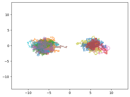
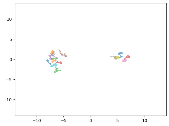
In Figure 2 we simulated the trajectories of Langevin dynamics with step size 0.0010.0010.001, again with initialization from samples and a learned score function, in a 32-dimensional mixture of Gaussians. Similar to the one-dimensional example, we can see that at moderate times the trajectories have mixed well within their component, and at large times the trajectories sometimes pass through the region in between the components where the true density is very small. Additional simulations (including an experiment with Contrastive Divergence training) and information is in Appendix I.
Refer to caption
(a) T=300𝑇300T=300
Refer to caption
(b) T=12000𝑇12000T=12000
Refer to caption
(c) T=120000𝑇120000T=120000
Figure 2: 2D projected trajectories of Langevin dynamics up to T𝑇T iterations with step size 0.0010.0010.001 in a 32-dimensional mixture of Gaussians 23​N​(−6​e1,1.5​I)+13​N​(6​e1,1.5​I)23𝑁6subscript𝑒11.5𝐼13𝑁6subscript𝑒11.5𝐼\frac{2}{3}N(-6e_{1},1.5I)+\frac{1}{3}N(6e_{1},1.5I). The projection is the first two coordinates and the direction of separation of the components is the first axis direction. Langevin is initialized from the empirical distribution (15 iid samples) and run with an approximate score function learned from samples using a one hidden-layer neural network.

References

  • Albergo et al. (2021) Michael S Albergo, Denis Boyda, Daniel C Hackett, Gurtej Kanwar, Kyle Cranmer, Sébastien Racaniere, Danilo Jimenez Rezende, and Phiala E Shanahan. Introduction to normalizing flows for lattice field theory. arXiv preprint arXiv:2101.08176, 2021.
  • Bakry et al. (2014) Dominique Bakry, Ivan Gentil, Michel Ledoux, et al. Analysis and geometry of Markov diffusion operators, volume 103. Springer, 2014.
  • Barp et al. (2019) Alessandro Barp, Francois-Xavier Briol, Andrew Duncan, Mark Girolami, and Lester Mackey. Minimum stein discrepancy estimators. Advances in Neural Information Processing Systems, 32, 2019.
  • Besag (1975) Julian Besag. Statistical analysis of non-lattice data. Journal of the Royal Statistical Society: Series D (The Statistician), 24(3):179–195, 1975.
  • Block et al. (2020) Adam Block, Youssef Mroueh, and Alexander Rakhlin. Generative modeling with denoising auto-encoders and langevin sampling. arXiv preprint arXiv:2002.00107, 2020.
  • Brennan et al. (2018) Matthew Brennan, Guy Bresler, and Wasim Huleihel. Reducibility and computational lower bounds for problems with planted sparse structure. In Conference On Learning Theory, pp.  48–166. PMLR, 2018.
  • Chen et al. (2021) Hong-Bin Chen, Sinho Chewi, and Jonathan Niles-Weed. Dimension-free log-sobolev inequalities for mixture distributions. Journal of Functional Analysis, 281(11):109236, 2021.
  • Chen et al. (2023) Sitan Chen, Sinho Chewi, Jerry Li, Yuanzhi Li, Adil Salim, and Anru R. Zhang. Sampling is as easy as learning the score: theory for diffusion models with minimal data assumptions, 2023.
  • Chewi et al. (2021) Sinho Chewi, Murat A. Erdogdu, Mufan Bill Li, Ruoqi Shen, and Matthew Zhang. Analysis of langevin monte carlo from poincaré to log-sobolev, 2021.
  • Dalalyan (2017) Arnak S Dalalyan. Theoretical guarantees for approximate sampling from smooth and log-concave densities. Journal of the Royal Statistical Society. Series B (Statistical Methodology), pp.  651–676, 2017.
  • Diaconis & Saloff-Coste (1996) Persi Diaconis and Laurent Saloff-Coste. Logarithmic sobolev inequalities for finite markov chains. The Annals of Applied Probability, 6(3):695–750, 1996.
  • Forbes & Lauritzen (2015) Peter GM Forbes and Steffen Lauritzen. Linear estimating equations for exponential families with application to gaussian linear concentration models. Linear Algebra and its Applications, 473:261–283, 2015.
  • Gao et al. (2018) Ruiqi Gao, Yang Lu, Junpei Zhou, Song-Chun Zhu, and Ying Nian Wu. Learning generative convnets via multi-grid modeling and sampling. In Proceedings of the IEEE Conference on Computer Vision and Pattern Recognition, pp.  9155–9164, 2018.
  • Ge et al. (2018) Rong Ge, Holden Lee, and Andrej Risteski. Simulated tempering langevin monte carlo ii: An improved proof using soft markov chain decomposition. arXiv preprint arXiv:1812.00793, 2018.
  • Hinton (2002) Geoffrey E Hinton. Training products of experts by minimizing contrastive divergence. Neural computation, 14(8):1771–1800, 2002.
  • Hinton (2012) Geoffrey E Hinton. A practical guide to training restricted boltzmann machines. Neural Networks: Tricks of the Trade: Second Edition, pp. 599–619, 2012.
  • Hyvärinen (2005) Aapo Hyvärinen. Estimation of non-normalized statistical models by score matching. Journal of Machine Learning Research, 6(4), 2005.
  • Hyvärinen (2007a) Aapo Hyvärinen. Connections between score matching, contrastive divergence, and pseudolikelihood for continuous-valued variables. IEEE Transactions on neural networks, 18(5):1529–1531, 2007a.
  • Hyvärinen (2007b) Aapo Hyvärinen. Some extensions of score matching. Computational statistics & data analysis, 51(5):2499–2512, 2007b.
  • Karatzas & Shreve (1991) Ioannis Karatzas and Steven E Shreve. Brownian motion and stochastic calculus, volume 113. Springer Science & Business Media, 1991.
  • Koehler et al. (2022) Frederic Koehler, Alexander Heckett, and Andrej Risteski. Statistical efficiency of score matching: The view from isoperimetry. arXiv preprint arXiv:2210.00726, 2022.
  • Lawrence & Yamauchi (2021) Scott Lawrence and Yukari Yamauchi. Normalizing flows and the real-time sign problem. Physical Review D, 103(11):114509, 2021.
  • Lee et al. (2018) Holden Lee, Andrej Risteski, and Rong Ge. Beyond log-concavity: Provable guarantees for sampling multi-modal distributions using simulated tempering langevin monte carlo. In S. Bengio, H. Wallach, H. Larochelle, K. Grauman, N. Cesa-Bianchi, and R. Garnett (eds.), Advances in Neural Information Processing Systems, volume 31. Curran Associates, Inc., 2018. URL https://proceedings.neurips.cc/paper/2018/file/c6ede20e6f597abf4b3f6bb30cee16c7-Paper.pdf.
  • Lee et al. (2022a) Holden Lee, Jianfeng Lu, and Yixin Tan. Convergence for score-based generative modeling with polynomial complexity. arXiv preprint arXiv:2206.06227, 2022a.
  • Lee et al. (2022b) Holden Lee, Jianfeng Lu, and Yixin Tan. Convergence of score-based generative modeling for general data distributions. arXiv preprint arXiv:2209.12381, 2022b.
  • Levin & Peres (2017) David A Levin and Yuval Peres. Markov chains and mixing times, volume 107. American Mathematical Soc., 2017.
  • Madras & Randall (2002) Neal Madras and Dana Randall. Markov chain decomposition for convergence rate analysis. Annals of Applied Probability, 12:581–606, 2002.
  • Mironov (2017) Ilya Mironov. Rényi differential privacy. In 2017 IEEE 30th computer security foundations symposium (CSF), pp.  263–275. IEEE, 2017.
  • Nijkamp et al. (2019) Erik Nijkamp, Mitch Hill, Song-Chun Zhu, and Ying Nian Wu. Learning non-convergent non-persistent short-run mcmc toward energy-based model. Advances in Neural Information Processing Systems, 32, 2019.
  • Nijkamp et al. (2020) Erik Nijkamp, Mitch Hill, Tian Han, Song-Chun Zhu, and Ying Nian Wu. On the anatomy of mcmc-based maximum likelihood learning of energy-based models. In Proceedings of the AAAI Conference on Artificial Intelligence, volume 34, pp.  5272–5280, 2020.
  • Rigollet & Hütter (2017) Phillippe Rigollet and Jan-Christian Hütter. High dimensional statistics. Lecture notes for course 18S997, 2017.
  • Rombach et al. (2022) Robin Rombach, Andreas Blattmann, Dominik Lorenz, Patrick Esser, and Björn Ommer. High-resolution image synthesis with latent diffusion models. In Proceedings of the IEEE/CVF Conference on Computer Vision and Pattern Recognition, pp.  10684–10695, 2022.
  • Schlichting (2019) André Schlichting. Poincaré and log–sobolev inequalities for mixtures. Entropy, 21(1):89, 2019. doi: 10.3390/e21010089. URL https://doi.org/10.3390%2Fe21010089.
  • Song & Ermon (2019) Yang Song and Stefano Ermon. Generative modeling by estimating gradients of the data distribution. Advances in Neural Information Processing Systems, 32, 2019.
  • Song et al. (2020a) Yang Song, Sahaj Garg, Jiaxin Shi, and Stefano Ermon. Sliced score matching: A scalable approach to density and score estimation. In Uncertainty in Artificial Intelligence, pp.  574–584. PMLR, 2020a.
  • Song et al. (2020b) Yang Song, Jascha Sohl-Dickstein, Diederik P Kingma, Abhishek Kumar, Stefano Ermon, and Ben Poole. Score-based generative modeling through stochastic differential equations. arXiv preprint arXiv:2011.13456, 2020b.
  • Sriperumbudur et al. (2017) Bharath Sriperumbudur, Kenji Fukumizu, Arthur Gretton, Aapo Hyvärinen, and Revant Kumar. Density estimation in infinite dimensional exponential families. Journal of Machine Learning Research, 18, 2017.
  • Tzen et al. (2018) Belinda Tzen, Tengyuan Liang, and Maxim Raginsky. Local optimality and generalization guarantees for the langevin algorithm via empirical metastability. In Conference On Learning Theory, pp.  857–875. PMLR, 2018.
  • Van Handel (2014) Ramon Van Handel. Probability in high dimension. Technical report, PRINCETON UNIV NJ, 2014.
  • Vempala & Wibisono (2019) Santosh Vempala and Andre Wibisono. Rapid convergence of the unadjusted langevin algorithm: Isoperimetry suffices. Advances in neural information processing systems, 32, 2019.
  • Vershynin (2018) Roman Vershynin. High-dimensional probability: An introduction with applications in data science, volume 47. Cambridge university press, 2018.
  • Vincent (2011) Pascal Vincent. A connection between score matching and denoising autoencoders. Neural computation, 23(7):1661–1674, 2011.
  • Wasserman (2006) Larry Wasserman. All of nonparametric statistics. Springer Science & Business Media, 2006.
  • Wenliang et al. (2019) Li Wenliang, Danica J Sutherland, Heiko Strathmann, and Arthur Gretton. Learning deep kernels for exponential family densities. In International Conference on Machine Learning, pp. 6737–6746. PMLR, 2019.
  • Xie et al. (2016) Jianwen Xie, Yang Lu, Song-Chun Zhu, and Yingnian Wu. A theory of generative convnet. In International Conference on Machine Learning, pp. 2635–2644. PMLR, 2016.

Appendix A Organization of Appendix

In Appendix B, we review some basic mathematical preliminaries and notation, such as the definition of log-Sobolev and Poincaré inequalities. In Appendix C we prove Theorem 4 (Theorem 2 of the main text), which shows that when clusters have significant overlap that the Langevin dynamics for the mixture distribution will successfully mix. Appendix D and Appendix E contain intermediate results which are used in the following sections: Appendix D shows how to analyze the Langevin diffusion starting from a point, and Appendix E shows how to bound the drift of the continuous Langevin diffusion over a short period of time. In Appendix F we prove Theorem 5, which shows that the continuous Langevin diffusion with score function ∇V∇𝑉\nabla V converges to μ𝜇\mu after a suitable time T.𝑇T. In Appendix G, we prove our main results Theorem 6 and Corollary 1, which show that the discrete LMC with score function s𝑠s with appropriately chosen step size is close to μ𝜇\mu in total variation distance at a suitable time. Corollary 1 corresponds to Theorem 1 of the main text. In Appendix H, we remove the dependency of the runtime and number of samples on the minimum weight of the components i.e. p∗=mini∈I⁡pisubscript𝑝subscript𝑖𝐼subscript𝑝𝑖p_{*}=\min_{i\in I}p_{i} (see Theorems 8 and 2 for the analogy of Theorems 6 and 1 respectively that has no dependency on p∗subscript𝑝p_{*}). Appendix I contains some additional simulations.

Appendix B Preliminaries

In the preliminaries, we review in more detail the needed background on divergences between probability measures, functional inequalities, log-concave distributions, etc. in order to prove our main results.

Notation.

We use standard big-Oh notation and use tildes, e.g. O~​(⋅)~𝑂⋅\tilde{O}(\cdot), to denote inequality up to log factors. We similarly use the notation ≲less-than-or-similar-to\lesssim to denote inequality up to a universal constant. We let dT​V​(μ,ν)=supA|μ​(A)−ν​(A)|subscript𝑑𝑇𝑉𝜇𝜈subscriptsupremum𝐴𝜇𝐴𝜈𝐴d_{TV}(\mu,\nu)=\sup_{A}|\mu(A)-\nu(A)| be the usual total variation distance between probability measures μ𝜇\mu and ν𝜈\nu defined on the same space, where the supremum ranges over measurable sets. Given a random variable X𝑋X, we write ℒ​(X)ℒ𝑋\mathcal{L}(X) to denote its law. In general, we use the same notation for a measure and its probability density function as long as there is no ambiguity. For random variables X,Z𝑋𝑍X,Z, we will write dT​V​(X,Z)subscript𝑑𝑇𝑉𝑋𝑍d_{TV}(X,Z) to denote the total variation distance between their laws ℒ​(X)ℒ𝑋\mathcal{L}(X) and ℒ​(Z).ℒ𝑍\mathcal{L}(Z).

B.1 Renyi divergence

The Renyi divergence, which generalizes the more well-known KL divergence, is a useful technical tool in the analysis of the Langevin diffusion — see e.g. Vempala & Wibisono (2019). The Renyi divergence of order q∈(1,∞)𝑞1q\in(1,\infty) of μ𝜇\mu from π𝜋\pi is defined to be

ℛq(μ||π)\displaystyle\mathcal{R}_{q}(\mu||\pi) =1q−1​ln⁡𝔼π​[(d​μ​(x)d​π​(x))q]=1q−1​ln​∫(d​μ​(x)d​π​(x))q​𝑑π​(x)absent1𝑞1subscript𝔼𝜋delimited-[]superscript𝑑𝜇𝑥𝑑𝜋𝑥𝑞1𝑞1superscript𝑑𝜇𝑥𝑑𝜋𝑥𝑞differential-d𝜋𝑥\displaystyle=\frac{1}{q-1}\ln\mathbb{E}_{\pi}\left[\left(\frac{d\mu(x)}{d\pi(x)}\right)^{q}\right]=\frac{1}{q-1}\ln\int\left(\frac{d\mu(x)}{d\pi(x)}\right)^{q}d\pi(x)
=1q−1​ln​∫(d​μ​(x)d​π​(x))q−1​𝑑μ​(x)=1q−1​ln⁡𝔼μ​[(d​μ​(x)d​π​(x))q−1]absent1𝑞1superscript𝑑𝜇𝑥𝑑𝜋𝑥𝑞1differential-d𝜇𝑥1𝑞1subscript𝔼𝜇delimited-[]superscript𝑑𝜇𝑥𝑑𝜋𝑥𝑞1\displaystyle=\frac{1}{q-1}\ln\int\left(\frac{d\mu(x)}{d\pi(x)}\right)^{q-1}d\mu(x)=\frac{1}{q-1}\ln\mathbb{E}_{\mu}\left[\left(\frac{d\mu(x)}{d\pi(x)}\right)^{q-1}\right]

The limit ℛqsubscriptℛ𝑞\mathcal{R}_{q} as q→1→𝑞1q\to 1 is the Kullback-Leibler divergence 𝒟KL(μ||π)=∫μ(x)logμ​(x)π​(x)dx,\mathcal{D}_{\operatorname{KL}}(\mu||\pi)=\int\mu(x)\log\frac{\mu(x)}{\pi(x)}dx, thus we write ℛ1​(⋅)=𝒟KL​(⋅).subscriptℛ1⋅subscript𝒟KL⋅\mathcal{R}_{1}(\cdot)=\mathcal{D}_{\operatorname{KL}}(\cdot). Renyi divergence increases as q𝑞q increases i.e. ℛq≤ℛq′subscriptℛ𝑞subscriptℛsuperscript𝑞′\mathcal{R}_{q}\leq\mathcal{R}_{q^{\prime}} for 1≤q≤q′.1𝑞superscript𝑞′1\leq q\leq q^{\prime}.

Lemma 1 (Weak triangle inequality, (Vempala & Wibisono, 2019, Lemma 7), Mironov (2017)).

For q>1𝑞1q>1 and any measure ν𝜈\nu absolutely continuous with respect to measure μ𝜇\mu,

ℛq(ν||μ)≤q−1/2q−1ℛ2​q(ν||ν′)+ℛ2​q−1(ν′||μ)\mathcal{R}_{q}(\nu||\mu)\leq\frac{q-1/2}{q-1}\mathcal{R}_{2q}(\nu||\nu^{\prime})+\mathcal{R}_{2q-1}(\nu^{\prime}||\mu)
Lemma 2 (Weak convexity of Renyi entropy).

For q>1𝑞1q>1, if μ𝜇\mu is a convex combination of μisubscript𝜇𝑖\mu_{i} i.e. μ​(x)=∑pi​μi​(x)𝜇𝑥subscript𝑝𝑖subscript𝜇𝑖𝑥\mu(x)=\sum p_{i}\mu_{i}(x) then

𝔼ν​[(d​ν​(x)d​μ​(x))q−1]≤∑ipi​𝔼ν​[(d​ν​(x)d​μi​(x))q−1].subscript𝔼𝜈delimited-[]superscript𝑑𝜈𝑥𝑑𝜇𝑥𝑞1subscript𝑖subscript𝑝𝑖subscript𝔼𝜈delimited-[]superscript𝑑𝜈𝑥𝑑subscript𝜇𝑖𝑥𝑞1\mathbb{E}_{\nu}\left[\left(\frac{d\nu(x)}{d\mu(x)}\right)^{q-1}\right]\leq\sum_{i}p_{i}\mathbb{E}_{\nu}\left[\left(\frac{d\nu(x)}{d\mu_{i}(x)}\right)^{q-1}\right].

Consequently, ℛq(ν||μ)≤maxiℛq(ν||μi)\mathcal{R}_{q}(\nu||\mu)\leq\max_{i}\mathcal{R}_{q}(\nu||\mu_{i}) and ℛq(μ||ν)≤maxiℛq(μi||ν)\mathcal{R}_{q}(\mu||\nu)\leq\max_{i}\mathcal{R}_{q}(\mu_{i}||\nu)

Proof.

By Holder’s inequality

(∑ipi​μi​(x))q−1​(∑i=1dpiμi​(x)q−1)≥(∑ipi)q=1superscriptsubscript𝑖subscript𝑝𝑖subscript𝜇𝑖𝑥𝑞1superscriptsubscript𝑖1𝑑subscript𝑝𝑖subscript𝜇𝑖superscript𝑥𝑞1superscriptsubscript𝑖subscript𝑝𝑖𝑞1(\sum_{i}p_{i}\mu_{i}(x))^{q-1}\left(\sum_{i=1}^{d}\frac{p_{i}}{\mu_{i}(x)^{q-1}}\right)\geq(\sum_{i}p_{i})^{q}=1

thus

(ν​(x)μ​(x))q−1≤∑ipi​(ν​(x)μi​(x))q−1superscript𝜈𝑥𝜇𝑥𝑞1subscript𝑖subscript𝑝𝑖superscript𝜈𝑥subscript𝜇𝑖𝑥𝑞1\left(\frac{\nu(x)}{\mu(x)}\right)^{q-1}\leq\sum_{i}p_{i}\left(\frac{\nu(x)}{\mu_{i}(x)}\right)^{q-1}

Taking expectation in ν𝜈\nu gives the first statement. Similarly, since q>1>0,𝑞10q>1>0,

𝔼ν​[(ν​(x)μ​(x))q]≤∑ipi​𝔼ν​[(ν​(x)μi​(x))q]subscript𝔼𝜈delimited-[]superscript𝜈𝑥𝜇𝑥𝑞subscript𝑖subscript𝑝𝑖subscript𝔼𝜈delimited-[]superscript𝜈𝑥subscript𝜇𝑖𝑥𝑞\mathbb{E}_{\nu}\left[\left(\frac{\nu(x)}{\mu(x)}\right)^{q}\right]\leq\sum_{i}p_{i}\mathbb{E}_{\nu}\left[\left(\frac{\nu(x)}{\mu_{i}(x)}\right)^{q}\right]

For the second statement

ℛq(ν||μ)=ln⁡𝔼ν​[(d​ν​(x)d​μ​(x))q−1]q−1≤ln⁡(maxi⁡𝔼ν​[(d​ν​(x)d​μi​(x))q−1])q−1=maxiℛq(ν||μi)\mathcal{R}_{q}(\nu||\mu)=\frac{\ln\mathbb{E}_{\nu}[(\frac{d\nu(x)}{d\mu(x)})^{q-1}]}{q-1}\leq\frac{\ln(\max_{i}\mathbb{E}_{\nu}[(\frac{d\nu(x)}{d\mu_{i}(x)})^{q-1}])}{q-1}=\max_{i}\mathcal{R}_{q}(\nu||\mu_{i})

and

ℛq(μ||ν)=ln⁡𝔼ν​[(d​ν​(x)d​μ​(x))q]q−1≤ln⁡(maxi⁡𝔼ν​[(d​ν​(x)d​μi​(x))q])q−1=maxiℛq(μi||ν).\mathcal{R}_{q}(\mu||\nu)=\frac{\ln\mathbb{E}_{\nu}[(\frac{d\nu(x)}{d\mu(x)})^{q}]}{q-1}\leq\frac{\ln(\max_{i}\mathbb{E}_{\nu}[(\frac{d\nu(x)}{d\mu_{i}(x)})^{q}])}{q-1}=\max_{i}\mathcal{R}_{q}(\mu_{i}||\nu).

∎

B.2 Log-concave distributions

Consider a density function π:ℝd→ℝ≥0:𝜋→superscriptℝ𝑑subscriptℝabsent0\pi:\mathbb{R}^{d}\to\mathbb{R}_{\geq 0} where π​(x)=exp⁡(−V​(x)).𝜋𝑥𝑉𝑥\pi(x)=\exp(-V(x)). Throughout the paper, we will assume V𝑉V is a twice continuously differentiable function. We say π𝜋\pi is β𝛽\beta-smooth if V𝑉V has bounded Hessian for all x∈ℝd𝑥superscriptℝ𝑑x\in\mathbb{R}^{d}:

−β​I⪯∇2V​(x)⪯β​I.precedes-or-equals𝛽𝐼superscript∇2𝑉𝑥precedes-or-equals𝛽𝐼-\beta I\preceq\nabla^{2}V(x)\preceq\beta I.

We say π𝜋\pi is α𝛼\alpha-strongly log-concave if

0≺α​I⪯∇2V​(x)precedes0𝛼𝐼precedes-or-equalssuperscript∇2𝑉𝑥0\prec\alpha I\preceq\nabla^{2}V(x)

for all x∈ℝd𝑥superscriptℝ𝑑x\in\mathbb{R}^{d}.

B.3 Functional inequalities

For nonnegative smooth f:ℝd→ℝ≥0,:𝑓→superscriptℝ𝑑subscriptℝabsent0f:\mathbb{R}^{d}\to\mathbb{R}_{\geq 0}, let the entropy of f𝑓f with respect to probability distribution π𝜋\pi be

Entπ⁡[f]=𝔼π​[f​ln⁡(f/𝔼π​[f])].subscriptEnt𝜋𝑓subscript𝔼𝜋delimited-[]𝑓𝑓subscript𝔼𝜋delimited-[]𝑓\operatorname{Ent}_{\pi}[f]=\mathbb{E}_{\pi}[f\ln(f/\mathbb{E}_{\pi}[f])].

We say π𝜋\pi satisfies a log-Sobolev inequality (LSI) with constant CL​Ssubscript𝐶𝐿𝑆C_{LS} if for all smooth functions f𝑓f,

Entπ⁡[f2]≤2​CL​S​𝔼π​[‖∇f‖2]subscriptEnt𝜋superscript𝑓22subscript𝐶𝐿𝑆subscript𝔼𝜋delimited-[]superscriptnorm∇𝑓2\operatorname{Ent}_{\pi}[f^{2}]\leq 2C_{LS}\mathbb{E}_{\pi}[||\nabla f||^{2}]

and π𝜋\pi satisfies a Poincare inequality (PI) with constant CP​Isubscript𝐶𝑃𝐼C_{PI} if Varπ⁡[f]≤2​CP​I​𝔼π​[‖∇f‖2]subscriptVar𝜋𝑓2subscript𝐶𝑃𝐼subscript𝔼𝜋delimited-[]superscriptnorm∇𝑓2\operatorname{Var}_{\pi}[f]\leq 2C_{PI}\mathbb{E}_{\pi}[||\nabla f||^{2}]. The log-Sobolev inequality implies Poincare inequality: CP​I≤CL​S.subscript𝐶𝑃𝐼subscript𝐶𝐿𝑆C_{PI}\leq C_{LS}. Due to the Bakry-Emery criterion, if π𝜋\pi is α𝛼\alpha-strongly log-concave then π𝜋\pi satisfies LSI with constant CL​S=1/α.subscript𝐶𝐿𝑆1𝛼C_{LS}=1/\alpha.

LSI and PI are equivalent to statements about exponential ergodicity of the continuous-time Langevin diffusion, which is defined by the Stochastic Differential Equation

d​X¯tπ=∇log⁡π​(X¯tμ)​d​t+2​d​Bt.𝑑superscriptsubscript¯𝑋𝑡𝜋∇𝜋superscriptsubscript¯𝑋𝑡𝜇𝑑𝑡2𝑑subscript𝐵𝑡d\bar{X}_{t}^{\pi}=\nabla\log\pi(\bar{X}_{t}^{\mu})\,dt+\sqrt{2}\,dB_{t}.

Specifically, let πtsubscript𝜋𝑡\pi_{t} denote the law of the diffusion at time t𝑡t initialized from π0subscript𝜋0\pi_{0} then a LSI is equivalent to the inequality

𝒟KL(πt||π)≤exp(−2t/CL​S)𝒟KL(π0||π)\mathcal{D}_{\operatorname{KL}}(\pi_{t}||\pi)\leq\exp(-2t/C_{LS})\mathcal{D}_{\operatorname{KL}}(\pi_{0}||\pi)

holding for an arbitrary initial distribution π0subscript𝜋0\pi_{0}. Similarly, a PI is equivalent to χ2(πt||π)≤exp(−2t/CP​I)χ2(π0||π)\chi^{2}(\pi_{t}||\pi)\leq\exp(-2t/C_{PI})\chi^{2}(\pi_{0}||\pi). Here 𝒟K​L​(P,Q)=𝔼P​[log⁡d​Pd​Q]subscript𝒟𝐾𝐿𝑃𝑄subscript𝔼𝑃delimited-[]𝑑𝑃𝑑𝑄\mathcal{D}_{KL}(P,Q)=\mathbb{E}_{P}[\log\frac{dP}{dQ}] is the Kullback-Liebler divergence and χ2​(P,Q)=𝔼Q​[(d​P/d​Q−1)2]superscript𝜒2𝑃𝑄subscript𝔼𝑄delimited-[]superscript𝑑𝑃𝑑𝑄12\chi^{2}(P,Q)=\mathbb{E}_{Q}[(dP/dQ-1)^{2}] is the χ2superscript𝜒2\chi^{2}-divergence. See Bakry et al. (2014); Van Handel (2014) for more background.

B.4 Concentration

Proposition 1 (Concentration of Brownian motion, (Chewi et al., 2021, Lemma 32)).

Let (Bt)t≥0subscriptsubscript𝐵𝑡𝑡0(B_{t})_{t\geq 0} be a standard Brownian motion in ℝdsuperscriptℝ𝑑\mathbb{R}^{d}. Then, if λ≥0𝜆0\lambda\geq 0 and h≤1/(4​λ),ℎ14𝜆h\leq 1/(4\lambda),

𝔼​[exp⁡(λ​supt∈[0,h]‖Bt‖2)]≤exp⁡(6​d​h​λ)𝔼delimited-[]𝜆subscriptsupremum𝑡0ℎsuperscriptnormsubscript𝐵𝑡26𝑑ℎ𝜆\mathbb{E}\left[\exp\left(\lambda\sup_{t\in[0,h]}||B_{t}||^{2}\right)\right]\leq\exp(6dh\lambda)

In particular, for all η≥0𝜂0\eta\geq 0

ℙ​[supt∈[0,h]‖Bt‖2≥η]≤exp⁡(−η26​d​h)ℙdelimited-[]subscriptsupremum𝑡0ℎsuperscriptnormsubscript𝐵𝑡2𝜂superscript𝜂26𝑑ℎ\mathbb{P}\left[\sup_{t\in[0,h]}||B_{t}||^{2}\geq\eta\right]\leq\exp\left(-\frac{\eta^{2}}{6dh}\right)
Proposition 2.

Suppose a random non-negative real variable Z𝑍Z satisfies

∀t:ℙ​[Z≥D+t]≤2​exp⁡(−γ​t2):for-all𝑡ℙdelimited-[]𝑍𝐷𝑡2𝛾superscript𝑡2\forall t:\mathbb{P}[Z\geq D+t]\leq 2\exp(-\gamma t^{2})

for some D≥0,γ>0.formulae-sequence𝐷0𝛾0D\geq 0,\gamma>0. Then there exists numerical constant C𝐶C s.t.

𝔼​[Zp]≤C​pp/2​(D+γ−1/2)p𝔼delimited-[]superscript𝑍𝑝𝐶superscript𝑝𝑝2superscript𝐷superscript𝛾12𝑝\mathbb{E}[Z^{p}]\leq Cp^{p/2}(D+\gamma^{-1/2})^{p}
Proof.

For some R≥D𝑅𝐷R\geq D to be chosen later

𝔼​[Zp]𝔼delimited-[]superscript𝑍𝑝\displaystyle\mathbb{E}[Z^{p}] =∫0∞ℙ​[Zp≥x]​𝑑xabsentsuperscriptsubscript0ℙdelimited-[]superscript𝑍𝑝𝑥differential-d𝑥\displaystyle=\int_{0}^{\infty}\mathbb{P}[Z^{p}\geq x]dx
=∫0Rpℙ​[Zp≥x]​𝑑x+∫Rp∞ℙ​[Zp≥x]​𝑑xabsentsuperscriptsubscript0superscript𝑅𝑝ℙdelimited-[]superscript𝑍𝑝𝑥differential-d𝑥superscriptsubscriptsuperscript𝑅𝑝ℙdelimited-[]superscript𝑍𝑝𝑥differential-d𝑥\displaystyle=\int_{0}^{R^{p}}\mathbb{P}[Z^{p}\geq x]dx+\int_{R^{p}}^{\infty}\mathbb{P}[Z^{p}\geq x]dx
≤∫0Rp1​𝑑x+∫R∞ℙ​[Z≥y]​d​(yp)absentsuperscriptsubscript0superscript𝑅𝑝1differential-d𝑥superscriptsubscript𝑅ℙdelimited-[]𝑍𝑦𝑑superscript𝑦𝑝\displaystyle\leq\int_{0}^{R^{p}}1dx+\int_{R}^{\infty}\mathbb{P}[Z\geq y]d(y^{p})
≤Rp+2​p​∫R∞yp−1​exp⁡(−γ​(y−D)2)​𝑑yabsentsuperscript𝑅𝑝2𝑝superscriptsubscript𝑅superscript𝑦𝑝1𝛾superscript𝑦𝐷2differential-d𝑦\displaystyle\leq R^{p}+2p\int_{R}^{\infty}y^{p-1}\exp(-\gamma(y-D)^{2})dy
≤Rp+p​2p​(∫R∞zp−1​exp⁡(−γ​z2)​𝑑z+Dp−1​∫R∞exp⁡(−γ​z2)​𝑑z)absentsuperscript𝑅𝑝𝑝superscript2𝑝superscriptsubscript𝑅superscript𝑧𝑝1𝛾superscript𝑧2differential-d𝑧superscript𝐷𝑝1superscriptsubscript𝑅𝛾superscript𝑧2differential-d𝑧\displaystyle\leq R^{p}+p2^{p}(\int_{R}^{\infty}z^{p-1}\exp(-\gamma z^{2})dz+D^{p-1}\int_{R}^{\infty}\exp(-\gamma z^{2})dz)
≤Rp+2p−1​(γ−p/2​(p/2)p/2+p​Dp−1​γ−1/2​π)absentsuperscript𝑅𝑝superscript2𝑝1superscript𝛾𝑝2superscript𝑝2𝑝2𝑝superscript𝐷𝑝1superscript𝛾12𝜋\displaystyle\leq R^{p}+2^{p-1}(\gamma^{-p/2}(p/2)^{p/2}+pD^{p-1}\gamma^{-1/2}\sqrt{\pi})

where in the last inequality, we make a change of variable u=γ​z2𝑢𝛾superscript𝑧2u=\gamma z^{2} and note that 2​p​∫zp−1​exp⁡(−γ​z2)​𝑑z=γ−p​p​∫up/2−1​exp⁡(−u)​𝑑u=Γ​(p/2)≤(p/2)p/22𝑝superscript𝑧𝑝1𝛾superscript𝑧2differential-d𝑧superscript𝛾𝑝𝑝superscript𝑢𝑝21𝑢differential-d𝑢Γ𝑝2superscript𝑝2𝑝22p\int z^{p-1}\exp(-\gamma z^{2})dz=\gamma^{-p}p\int u^{p/2-1}\exp(-u)du=\Gamma(p/2)\leq(p/2)^{p/2} and ∫0∞exp⁡(−γ​z2)​𝑑z=(2​γ)−1/2​2​π/2.superscriptsubscript0𝛾superscript𝑧2differential-d𝑧superscript2𝛾122𝜋2\int_{0}^{\infty}\exp(-\gamma z^{2})dz=(2\gamma)^{-1/2}\sqrt{2\pi}/2. Take R=D𝑅𝐷R=D gives the desired result. ∎

Proposition 3 ((Bakry et al., 2014, 5.4.2), restated in (Lee et al., 2022a, Lemma E.2) ).

Suppose π:ℝd→ℝ≥0:𝜋→superscriptℝ𝑑subscriptℝabsent0\pi:\mathbb{R}^{d}\to\mathbb{R}_{\geq 0} satisfies LSI with constant 1/α.1𝛼1/\alpha. Let f:ℝd→ℝ:𝑓→superscriptℝ𝑑ℝf:\mathbb{R}^{d}\to\mathbb{R} be a L𝐿L-Lipschitz function then

ℙx∼π​[|f​(x)−𝔼π​[f​(x)]|≥t]≤exp⁡(−α​t22​L2)subscriptℙsimilar-to𝑥𝜋delimited-[]𝑓𝑥subscript𝔼𝜋delimited-[]𝑓𝑥𝑡𝛼superscript𝑡22superscript𝐿2\mathbb{P}_{x\sim\pi}[|f(x)-\mathbb{E}_{\pi}[f(x)]|\geq t]\leq\exp\left(-\frac{\alpha t^{2}}{2L^{2}}\right)
Proposition 4 (Sub-Gaussian concentration of norm for strongly log concave measures).

Let V:ℝd→ℝ:𝑉→superscriptℝ𝑑ℝV:\mathbb{R}^{d}\to\mathbb{R} be a α𝛼\alpha-strongly convex and β𝛽\beta-smooth function. Let κ=β/α.𝜅𝛽𝛼\kappa=\beta/\alpha. Let π𝜋\pi be the probability measure with π​(x)∝exp⁡(−V​(x)).proportional-to𝜋𝑥𝑉𝑥\pi(x)\propto\exp(-V(x)). Let x∗=arg⁡minx⁡V​(x)subscript𝑥subscript𝑥𝑉𝑥x_{*}=\arg\min_{x}V(x) then for D=5​dα​ln⁡(10​κ)𝐷5𝑑𝛼10𝜅D=5\sqrt{\frac{d}{\alpha}}\ln(10\kappa) we have

ℙx∼π​[‖x−x∗‖≥D+t]≤exp⁡(−α​t2/4)subscriptℙsimilar-to𝑥𝜋delimited-[]norm𝑥subscript𝑥𝐷𝑡𝛼superscript𝑡24\mathbb{P}_{x\sim\pi}[||x-x_{*}||\geq D+t]\leq\exp(-\alpha t^{2}/4)

thus by Proposition 2, for p≥1.𝑝1p\geq 1.

𝔼π[||x−x∗||p]1/p≤O(1)pdαln(10κ)p\mathbb{E}_{\pi}[||x-x^{*}||^{p}]^{1/p}\leq O(1)\sqrt{p}\sqrt{\frac{d}{\alpha}}\ln(10\kappa)^{p}
Proof.

By (Lee et al., 2022a, Lemma E.3), let x¯=𝔼π​[x]¯𝑥subscript𝔼𝜋delimited-[]𝑥\bar{x}=\mathbb{E}_{\pi}[x] then ‖x¯−x∗‖≤12​dα​ln⁡(10​κ).norm¯𝑥superscript𝑥12𝑑𝛼10𝜅||\bar{x}-x^{*}||\leq\frac{1}{2}\sqrt{\frac{d}{\alpha}}\ln(10\kappa). By Proposition 3, for any unit vector v∈ℝd,𝑣superscriptℝ𝑑v\in\mathbb{R}^{d}, the function ⟨v,x−x¯⟩𝑣𝑥¯𝑥\langle v,x-\bar{x}\rangle is 1-Lipschitz, since |⟨v,x⟩−⟨v,y⟩|≤‖v‖2​‖x−y‖2=‖x−y‖2.𝑣𝑥𝑣𝑦subscriptnorm𝑣2subscriptnorm𝑥𝑦2subscriptnorm𝑥𝑦2|\langle v,x\rangle-\langle v,y\rangle|\leq\sqrt{||v||_{2}}||x-y||_{2}=||x-y||_{2}. Thus, by Proposition 3, ⟨v,x−x¯⟩𝑣𝑥¯𝑥\langle v,x-\bar{x}\rangle has mean 00 and sub-Gaussian concentration for all unit vector v,𝑣v, thus x−x¯⟩x-\bar{x}\rangle is a sub-Gaussian random vector. From sub-Gaussianity, a standard argument (see e.g. Theorem 1.19 of Rigollet & Hütter (2017)) shows that

ℙπ​[‖x−x¯‖≥4​dα+t]≤exp⁡(−α​t2/4)subscriptℙ𝜋delimited-[]norm𝑥¯𝑥4𝑑𝛼𝑡𝛼superscript𝑡24\mathbb{P}_{\pi}\left[||x-\bar{x}||\geq 4\sqrt{\frac{d}{\alpha}}+t\right]\leq\exp(-\alpha t^{2}/4)

thus by triangle inequality, using that ‖x¯−x∗‖≤dα​12​ln⁡(10​κ)norm¯𝑥superscript𝑥𝑑𝛼1210𝜅||\bar{x}-x^{*}||\leq\sqrt{\frac{d}{\alpha}}\frac{1}{2}\ln(10\kappa), we have

ℙπ​[‖x−x∗‖≥(4+1/2​ln⁡(10​κ))​dα+t]≤ℙπ​[‖x−x¯‖≥4​dα+t]≤exp⁡(−α​t2/4)subscriptℙ𝜋delimited-[]norm𝑥superscript𝑥41210𝜅𝑑𝛼𝑡subscriptℙ𝜋delimited-[]norm𝑥¯𝑥4𝑑𝛼𝑡𝛼superscript𝑡24\mathbb{P}_{\pi}\left[||x-x^{*}||\geq(4+1/2\ln(10\kappa))\sqrt{\frac{d}{\alpha}}+t\right]\leq\mathbb{P}_{\pi}\left[||x-\bar{x}||\geq 4\sqrt{\frac{d}{\alpha}}+t\right]\leq\exp(-\alpha t^{2}/4)

∎

Proposition 5 (Normalization factor bound).

Let V:ℝd→ℝ:𝑉→superscriptℝ𝑑ℝV:\mathbb{R}^{d}\to\mathbb{R} be a α𝛼\alpha-strongly convex and β𝛽\beta-smooth function. Let π𝜋\pi be the probability measure defined by π​(x)∝exp⁡(−V​(x))proportional-to𝜋𝑥𝑉𝑥\pi(x)\propto\exp(-V(x)) and Z:=Zπ=∫exp⁡(−V​(x))​𝑑xassign𝑍subscript𝑍𝜋𝑉𝑥differential-d𝑥Z:=Z_{\pi}=\int\exp(-V(x))dx be its normalization factor. For any y∈ℝd𝑦superscriptℝ𝑑y\in\mathbb{R}^{d}

exp⁡(−V​(y)+‖∇V​(y)‖22​β)​(2​π​β−1)d/2≤Z≤exp⁡(−V​(y)+‖∇V​(y)‖22​α)​(2​π​α−1)d/2𝑉𝑦superscriptnorm∇𝑉𝑦22𝛽superscript2𝜋superscript𝛽1𝑑2𝑍𝑉𝑦superscriptnorm∇𝑉𝑦22𝛼superscript2𝜋superscript𝛼1𝑑2\exp\left(-V(y)+\frac{||\nabla V(y)||^{2}}{2\beta}\right)(2\pi\beta^{-1})^{d/2}\leq Z\leq\exp\left(-V(y)+\frac{||\nabla V(y)||^{2}}{2\alpha}\right)(2\pi\alpha^{-1})^{d/2}

Let y=x∗=arg⁡min⁡V​(x)𝑦superscript𝑥𝑉𝑥y=x^{*}=\arg\min V(x) and assume w.l.o.g. V​(y)=0𝑉𝑦0V(y)=0 gives

d2​ln⁡1β≤ln⁡Zπ−d2​ln⁡(2​π)≤d2​ln⁡1α𝑑21𝛽subscript𝑍𝜋𝑑22𝜋𝑑21𝛼\frac{d}{2}\ln\frac{1}{\beta}\leq\ln Z_{\pi}-\frac{d}{2}\ln(2\pi)\leq\frac{d}{2}\ln\frac{1}{\alpha}
Proof.

Since α​I⪯∇2V​(x)⪯β​I,precedes-or-equals𝛼𝐼superscript∇2𝑉𝑥precedes-or-equals𝛽𝐼\alpha I\preceq\nabla^{2}V(x)\preceq\beta I,

⟨∇V​(y),x−y⟩+α​‖x−y‖2/2≤V​(x)−V​(y)≤⟨∇V​(y),x−y⟩+β​‖x−y‖2/2∇𝑉𝑦𝑥𝑦𝛼superscriptnorm𝑥𝑦22𝑉𝑥𝑉𝑦∇𝑉𝑦𝑥𝑦𝛽superscriptnorm𝑥𝑦22\langle\nabla V(y),x-y\rangle+\alpha||x-y||^{2}/2\leq V(x)-V(y)\leq\langle\nabla V(y),x-y\rangle+\beta||x-y||^{2}/2
Z𝑍\displaystyle Z ≤∫exp⁡(−V​(y)−⟨∇V​(y),x−y⟩−α​‖x−y‖2/2)​𝑑xabsent𝑉𝑦∇𝑉𝑦𝑥𝑦𝛼superscriptnorm𝑥𝑦22differential-d𝑥\displaystyle\leq\int\exp(-V(y)-\langle\nabla V(y),x-y\rangle-\alpha||x-y||^{2}/2)dx
=exp⁡(−V​(y)+‖∇V​(y)‖22​α)​∫exp⁡(−α​‖(x−y)+α−1​∇V​(y)‖22)​𝑑xabsent𝑉𝑦superscriptnorm∇𝑉𝑦22𝛼𝛼superscriptnorm𝑥𝑦superscript𝛼1∇𝑉𝑦22differential-d𝑥\displaystyle=\exp\left(-V(y)+\frac{||\nabla V(y)||^{2}}{2\alpha}\right)\int\exp\left(-\frac{\alpha||(x-y)+\alpha^{-1}\nabla V(y)||^{2}}{2}\right)dx
=exp⁡(−V​(y)+‖∇V​(y)‖22​α)​(2​π​α−1)d/2absent𝑉𝑦superscriptnorm∇𝑉𝑦22𝛼superscript2𝜋superscript𝛼1𝑑2\displaystyle=\exp\left(-V(y)+\frac{||\nabla V(y)||^{2}}{2\alpha}\right)(2\pi\alpha^{-1})^{d/2}

The lower bound follows similarly. The second statement follows from the first since ∇V​(x∗)=0.∇𝑉superscript𝑥0\nabla V(x^{*})=0.

∎

B.5 Girsanov’s theorem

Theorem 3 (Girsanov’s Theorem (Karatzas & Shreve, 1991, Chapter 3.5)).

Let (Xt)t≥0subscriptsubscript𝑋𝑡𝑡0(X_{t})_{t\geq 0} be stochastic processes adapted to the same filtration. Let PTsubscript𝑃𝑇P_{T} and QTsubscript𝑄𝑇Q_{T} be probability measure on the path space C​([0,T];ℝd)𝐶0𝑇superscriptℝ𝑑C([0,T];\mathbb{R}^{d}) s.t. Xtsubscript𝑋𝑡X_{t} evolved according to

d​Xt𝑑subscript𝑋𝑡\displaystyle dX_{t} =btP​d​t+2​d​BtP​ under ​PTabsentsubscriptsuperscript𝑏𝑃𝑡𝑑𝑡2𝑑superscriptsubscript𝐵𝑡𝑃 under subscript𝑃𝑇\displaystyle=b^{P}_{t}dt+\sqrt{2}dB_{t}^{P}\text{ under }P_{T}
d​Xt𝑑subscript𝑋𝑡\displaystyle dX_{t} =btQ​d​t+2​d​BtQ​ under ​QTabsentsubscriptsuperscript𝑏𝑄𝑡𝑑𝑡2𝑑superscriptsubscript𝐵𝑡𝑄 under subscript𝑄𝑇\displaystyle=b^{Q}_{t}dt+\sqrt{2}dB_{t}^{Q}\text{ under }Q_{T}

Assume that Novikov’s condition

𝔼QT​[exp⁡(14​∫0T‖btP−btQ‖2​𝑑t)]<∞subscript𝔼subscript𝑄𝑇delimited-[]14superscriptsubscript0𝑇superscriptnormsubscriptsuperscript𝑏𝑃𝑡subscriptsuperscript𝑏𝑄𝑡2differential-d𝑡\mathbb{E}_{Q_{T}}\left[\exp\left(\frac{1}{4}\int_{0}^{T}||b^{P}_{t}-b^{Q}_{t}||^{2}dt\right)\right]<\infty (5)

holds. Then

d​PTd​QT=exp⁡(∫0T12​⟨btP−btQ,d​BtQ⟩−14​∫0T‖btP−btQ‖2​𝑑t)𝑑subscript𝑃𝑇𝑑subscript𝑄𝑇superscriptsubscript0𝑇12subscriptsuperscript𝑏𝑃𝑡subscriptsuperscript𝑏𝑄𝑡𝑑superscriptsubscript𝐵𝑡𝑄14superscriptsubscript0𝑇superscriptnormsubscriptsuperscript𝑏𝑃𝑡subscriptsuperscript𝑏𝑄𝑡2differential-d𝑡\frac{dP_{T}}{dQ_{T}}=\exp\left(\int_{0}^{T}\frac{1}{\sqrt{2}}\langle b^{P}_{t}-b^{Q}_{t},dB_{t}^{Q}\rangle-\frac{1}{4}\int_{0}^{T}||b^{P}_{t}-b^{Q}_{t}||^{2}dt\right) (6)
Lemma 3 (Application of Girsanov with approximation argument (Chen et al., 2023, Equation 5.5, Proof of Theorem 9)).

Let (Xt)t≥0subscriptsubscript𝑋𝑡𝑡0(X_{t})_{t\geq 0} be stochastic processes adapted to the same filtration. Let PTsubscript𝑃𝑇P_{T} and QTsubscript𝑄𝑇Q_{T} be probability measure on the path space C​([0,T];ℝd)𝐶0𝑇superscriptℝ𝑑C([0,T];\mathbb{R}^{d}) s.t. Xtsubscript𝑋𝑡X_{t} evolved according to

d​Xt𝑑subscript𝑋𝑡\displaystyle dX_{t} =btP​d​t+2​d​BtP​ under ​PTabsentsubscriptsuperscript𝑏𝑃𝑡𝑑𝑡2𝑑superscriptsubscript𝐵𝑡𝑃 under subscript𝑃𝑇\displaystyle=b^{P}_{t}dt+\sqrt{2}dB_{t}^{P}\text{ under }P_{T}
d​Xt𝑑subscript𝑋𝑡\displaystyle dX_{t} =btQ​d​t+2​d​BtQ​ under ​QTabsentsubscriptsuperscript𝑏𝑄𝑡𝑑𝑡2𝑑superscriptsubscript𝐵𝑡𝑄 under subscript𝑄𝑇\displaystyle=b^{Q}_{t}dt+\sqrt{2}dB_{t}^{Q}\text{ under }Q_{T}

Suppose 𝔼QT​[∫0T‖btP−btQ‖2​𝑑t]<∞subscript𝔼subscript𝑄𝑇delimited-[]superscriptsubscript0𝑇superscriptnormsubscriptsuperscript𝑏𝑃𝑡subscriptsuperscript𝑏𝑄𝑡2differential-d𝑡\mathbb{E}_{Q_{T}}[\int_{0}^{T}||b^{P}_{t}-b^{Q}_{t}||^{2}dt]<\infty then

2dT​V(QT||PT)2≤𝒟KL(QT||PT)≤𝔼QT[∫0T||btP−btQ||2dt]2d_{TV}(Q_{T}||P_{T})^{2}\leq\mathcal{D}_{\operatorname{KL}}(Q_{T}||P_{T})\leq\mathbb{E}_{Q_{T}}\left[\int_{0}^{T}||b^{P}_{t}-b^{Q}_{t}||^{2}dt\right]
Lemma 4 (Corollary of Theorem 3, (Chewi et al., 2021, Corollary 20)).

With the setup and preconditions in Theorem 3, For any event ℰ,ℰ\mathcal{E},

𝔼QT​[(d​PTd​QT)q​1ℰ]≤𝔼QT​[exp⁡(q2​∫0T‖btP−btQ‖2​𝑑t)​1ℰ]subscript𝔼subscript𝑄𝑇delimited-[]superscript𝑑subscript𝑃𝑇𝑑subscript𝑄𝑇𝑞subscript1ℰsubscript𝔼subscript𝑄𝑇delimited-[]superscript𝑞2superscriptsubscript0𝑇superscriptnormsubscriptsuperscript𝑏𝑃𝑡subscriptsuperscript𝑏𝑄𝑡2differential-d𝑡subscript1ℰ\mathbb{E}_{Q_{T}}\left[\left(\frac{dP_{T}}{dQ_{T}}\right)^{q}\textbf{1}_{\mathcal{E}}\right]\leq\sqrt{\mathbb{E}_{Q_{T}}\left[\exp\left(q^{2}\int_{0}^{T}||b^{P}_{t}-b^{Q}_{t}||^{2}dt\right)\textbf{1}_{\mathcal{E}}\right]}

B.6 Mixture potential

Notation for indexing components.

Let I=[K]𝐼delimited-[]𝐾I=[K] be the set of indices i𝑖i for the components μisubscript𝜇𝑖\mu_{i} of the mixture distribution μ𝜇\mu. We will need to work with subsets S𝑆S of I𝐼I and the mixture distribution forms by components μisubscript𝜇𝑖\mu_{i} for i∈S.𝑖𝑆i\in S.

Definition 2.

For S⊆I,𝑆𝐼S\subseteq I, let pS=∑i∈Spi,subscript𝑝𝑆subscript𝑖𝑆subscript𝑝𝑖p_{S}=\sum_{i\in S}p_{i}, and μS=pS−1​∑i∈Spi​μi.subscript𝜇𝑆superscriptsubscript𝑝𝑆1subscript𝑖𝑆subscript𝑝𝑖subscript𝜇𝑖\mu_{S}=p_{S}^{-1}\sum_{i\in S}p_{i}\mu_{i}. Let VS=−log⁡μS.subscript𝑉𝑆subscript𝜇𝑆V_{S}=-\log\mu_{S}.

If S=I𝑆𝐼S=I we omit the subscript S.𝑆S.

Derivative computations.

For future use, we compute the derivatives of V.𝑉V.

Proposition 6 (Gradient of V𝑉V).
∇V​(x)=∑pi​μi​(x)​∇Vi​(x)μ​(x)∇𝑉𝑥subscript𝑝𝑖subscript𝜇𝑖𝑥∇subscript𝑉𝑖𝑥𝜇𝑥\nabla V(x)=\frac{\sum p_{i}\mu_{i}(x)\nabla V_{i}(x)}{\mu(x)} (7)

Consequently, ‖∇V​(x)‖≤max​‖∇Vi​(x)‖.norm∇𝑉𝑥norm∇subscript𝑉𝑖𝑥||\nabla V(x)||\leq\max||\nabla V_{i}(x)||.

Proof.

The statement follows from

∇V​(x)=∇log⁡μ​(x)=∇μ​(x)μ​(x)∇𝑉𝑥∇𝜇𝑥∇𝜇𝑥𝜇𝑥\displaystyle\nabla V(x)=\nabla\log\mu(x)=\frac{\nabla\mu(x)}{\mu(x)}

and

∇μ(x)=∇(∑piZi−1exp(−Vi(x))=−∑piμi(x)∇Vi(x).\displaystyle\nabla\mu(x)=\nabla(\sum p_{i}Z_{i}^{-1}\exp(-V_{i}(x))=-\sum p_{i}\mu_{i}(x)\nabla V_{i}(x).

∎

Proposition 7 (Hessian of V𝑉V).
∇2V​(x)=∑ipi​μi​(x)​∇2Vi​(x)μ​(x)−∑i,jpi​pj​μi​(x)​μj​(x)​(∇Vi​(x)−∇Vj​(x))​(∇Vi​(x)−∇Vj​(x))⊤4​μ2​(x)superscript∇2𝑉𝑥subscript𝑖subscript𝑝𝑖subscript𝜇𝑖𝑥superscript∇2subscript𝑉𝑖𝑥𝜇𝑥subscript𝑖𝑗subscript𝑝𝑖subscript𝑝𝑗subscript𝜇𝑖𝑥subscript𝜇𝑗𝑥∇subscript𝑉𝑖𝑥∇subscript𝑉𝑗𝑥superscript∇subscript𝑉𝑖𝑥∇subscript𝑉𝑗𝑥top4superscript𝜇2𝑥\nabla^{2}V(x)=\frac{\sum_{i}p_{i}\mu_{i}(x)\nabla^{2}V_{i}(x)}{\mu(x)}-\sum_{i,j}\frac{p_{i}p_{j}\mu_{i}(x)\mu_{j}(x)(\nabla V_{i}(x)-\nabla V_{j}(x))(\nabla V_{i}(x)-\nabla V_{j}(x))^{\top}}{4\mu^{2}(x)} (8)

hence if ∇2Vi⪯β​Iprecedes-or-equalssuperscript∇2subscript𝑉𝑖𝛽𝐼\nabla^{2}V_{i}\preceq\beta I for all i∈I𝑖𝐼i\in I then ∇2V​(x)⪯β​I.precedes-or-equalssuperscript∇2𝑉𝑥𝛽𝐼\nabla^{2}V(x)\preceq\beta I.

Proof.

Let Zi=∫exp⁡(−Vi​(x))​𝑑xsubscript𝑍𝑖subscript𝑉𝑖𝑥differential-d𝑥Z_{i}=\int\exp(-V_{i}(x))dx be the normalization factor of μi.subscript𝜇𝑖\mu_{i}. Note that

∇(μi​(x)​∇Vi​(x))∇subscript𝜇𝑖𝑥∇subscript𝑉𝑖𝑥\displaystyle\nabla(\mu_{i}(x)\nabla V_{i}(x))
=∇(Zi−1​exp⁡(−Vi​(X))​∇Vi​(x))=Zi−1​exp⁡(−Vi​(x))​(−∇Vi​(x)​∇Vi​(x)⊤+∇2Vi​(x))absent∇superscriptsubscript𝑍𝑖1subscript𝑉𝑖𝑋∇subscript𝑉𝑖𝑥superscriptsubscript𝑍𝑖1subscript𝑉𝑖𝑥∇subscript𝑉𝑖𝑥∇subscript𝑉𝑖superscript𝑥topsuperscript∇2subscript𝑉𝑖𝑥\displaystyle=\nabla(Z_{i}^{-1}\exp(-V_{i}(X))\nabla V_{i}(x))=Z_{i}^{-1}\exp(-V_{i}(x))(-\nabla V_{i}(x)\nabla V_{i}(x)^{\top}+\nabla^{2}V_{i}(x))
=μi​(x)​(∇2Vi​(x)−∇Vi​(x)​∇Vi​(x)⊤)absentsubscript𝜇𝑖𝑥superscript∇2subscript𝑉𝑖𝑥∇subscript𝑉𝑖𝑥∇subscript𝑉𝑖superscript𝑥top\displaystyle=\mu_{i}(x)(\nabla^{2}V_{i}(x)-\nabla V_{i}(x)\nabla V_{i}(x)^{\top})

and ∇μ​(x)=−∑pi​μi​(x)​∇Vi​(x),∇𝜇𝑥subscript𝑝𝑖subscript𝜇𝑖𝑥∇subscript𝑉𝑖𝑥\nabla\mu(x)=-\sum p_{i}\mu_{i}(x)\nabla V_{i}(x), thus

∇2V​(x)superscript∇2𝑉𝑥\displaystyle\nabla^{2}V(x)
=∇(∑ipi​μi​(x)​∇Vi​(x))μ​(x)−(∑pi​μi​(x)​∇Vi​(x))​∇μ​(x)μ2​(x)absent∇subscript𝑖subscript𝑝𝑖subscript𝜇𝑖𝑥∇subscript𝑉𝑖𝑥𝜇𝑥subscript𝑝𝑖subscript𝜇𝑖𝑥∇subscript𝑉𝑖𝑥∇𝜇𝑥superscript𝜇2𝑥\displaystyle=\frac{\nabla(\sum_{i}p_{i}\mu_{i}(x)\nabla V_{i}(x))}{\mu(x)}-\frac{(\sum p_{i}\mu_{i}(x)\nabla V_{i}(x))\nabla\mu(x)}{\mu^{2}(x)}
=∑pi​μi​(x)​(∇2Vi​(x)−∇Vi​(x)​∇Vi​(x)⊤)μ​(x)+(∑pi​μi​(x)​∇Vi​(x))​(∑pi​μi​(x)​∇Vi​(x))⊤μ2​(x)absentsubscript𝑝𝑖subscript𝜇𝑖𝑥superscript∇2subscript𝑉𝑖𝑥∇subscript𝑉𝑖𝑥∇subscript𝑉𝑖superscript𝑥top𝜇𝑥subscript𝑝𝑖subscript𝜇𝑖𝑥∇subscript𝑉𝑖𝑥superscriptsubscript𝑝𝑖subscript𝜇𝑖𝑥∇subscript𝑉𝑖𝑥topsuperscript𝜇2𝑥\displaystyle=\frac{\sum p_{i}\mu_{i}(x)(\nabla^{2}V_{i}(x)-\nabla V_{i}(x)\nabla V_{i}(x)^{\top})}{\mu(x)}+\frac{(\sum p_{i}\mu_{i}(x)\nabla V_{i}(x))(\sum p_{i}\mu_{i}(x)\nabla V_{i}(x))^{\top}}{\mu^{2}(x)}

Next,

(∑pi​μi​(x)​∇Vi​(x))​(∑pi​μi​(x)​∇Vi​(x))⊤−(∑pi​μi​∇Vi​(x)​∇Vi​(x)⊤)​(∑pi​μi)subscript𝑝𝑖subscript𝜇𝑖𝑥∇subscript𝑉𝑖𝑥superscriptsubscript𝑝𝑖subscript𝜇𝑖𝑥∇subscript𝑉𝑖𝑥topsubscript𝑝𝑖subscript𝜇𝑖∇subscript𝑉𝑖𝑥∇subscript𝑉𝑖superscript𝑥topsubscript𝑝𝑖subscript𝜇𝑖\displaystyle(\sum p_{i}\mu_{i}(x)\nabla V_{i}(x))(\sum p_{i}\mu_{i}(x)\nabla V_{i}(x))^{\top}-(\sum p_{i}\mu_{i}\nabla V_{i}(x)\nabla V_{i}(x)^{\top})(\sum p_{i}\mu_{i})
=∑i,jpi​pj​μi​(x)​μj​(x)​∇Vi​(x)​∇Vj⊤−∑i,jpi​pj​μi​(x)​μj​(x)​∇Vi​(x)​∇Vi​(x)⊤absentsubscript𝑖𝑗subscript𝑝𝑖subscript𝑝𝑗subscript𝜇𝑖𝑥subscript𝜇𝑗𝑥∇subscript𝑉𝑖𝑥∇superscriptsubscript𝑉𝑗topsubscript𝑖𝑗subscript𝑝𝑖subscript𝑝𝑗subscript𝜇𝑖𝑥subscript𝜇𝑗𝑥∇subscript𝑉𝑖𝑥∇subscript𝑉𝑖superscript𝑥top\displaystyle=\sum_{i,j}p_{i}p_{j}\mu_{i}(x)\mu_{j}(x)\nabla V_{i}(x)\nabla V_{j}^{\top}-\sum_{i,j}p_{i}p_{j}\mu_{i}(x)\mu_{j}(x)\nabla V_{i}(x)\nabla V_{i}(x)^{\top}
=12​∑i≠jpi​pj​μi​(x)​μj​(x)​(∇Vi​(x)​∇Vj⊤+∇Vj​(x)​∇Vi⊤−∇Vi​(x)​∇Vi⊤−∇Vj​(x)​∇Vj⊤)absent12subscript𝑖𝑗subscript𝑝𝑖subscript𝑝𝑗subscript𝜇𝑖𝑥subscript𝜇𝑗𝑥∇subscript𝑉𝑖𝑥∇superscriptsubscript𝑉𝑗top∇subscript𝑉𝑗𝑥∇superscriptsubscript𝑉𝑖top∇subscript𝑉𝑖𝑥∇superscriptsubscript𝑉𝑖top∇subscript𝑉𝑗𝑥∇superscriptsubscript𝑉𝑗top\displaystyle=\frac{1}{2}\sum_{i\neq j}p_{i}p_{j}\mu_{i}(x)\mu_{j}(x)(\nabla V_{i}(x)\nabla V_{j}^{\top}+\nabla V_{j}(x)\nabla V_{i}^{\top}-\nabla V_{i}(x)\nabla V_{i}^{\top}-\nabla V_{j}(x)\nabla V_{j}^{\top})
=−12​∑i≠jpi​pj​μi​(x)​μj​(x)​(∇Vi​(x)−∇Vj​(x))​(∇Vi​(X)−∇Vj​(x))⊤absent12subscript𝑖𝑗subscript𝑝𝑖subscript𝑝𝑗subscript𝜇𝑖𝑥subscript𝜇𝑗𝑥∇subscript𝑉𝑖𝑥∇subscript𝑉𝑗𝑥superscript∇subscript𝑉𝑖𝑋∇subscript𝑉𝑗𝑥top\displaystyle=-\frac{1}{2}\sum_{i\neq j}p_{i}p_{j}\mu_{i}(x)\mu_{j}(x)(\nabla V_{i}(x)-\nabla V_{j}(x))(\nabla V_{i}(X)-\nabla V_{j}(x))^{\top}

thus the first statement follows. The second statement follows from noticing that (∇Vi​(x)−∇Vj​(x))​(∇Vi​(X)−∇Vj​(x))⊤⪰0.succeeds-or-equals∇subscript𝑉𝑖𝑥∇subscript𝑉𝑗𝑥superscript∇subscript𝑉𝑖𝑋∇subscript𝑉𝑗𝑥top0(\nabla V_{i}(x)-\nabla V_{j}(x))(\nabla V_{i}(X)-\nabla V_{j}(x))^{\top}\succeq 0. ∎

B.7 Properties of smooth and strongly log-concave distribution

We record the consequences of α𝛼\alpha-strongly log-concave and β𝛽\beta-smooth that we will use.

Lemma 5.

Suppose μisubscript𝜇𝑖\mu_{i} is α𝛼\alpha-strongly log-concave and β𝛽\beta-smooth then for κ=β/α,𝜅𝛽𝛼\kappa=\beta/\alpha, ui=arg⁡min⁡Vi​(x),subscript𝑢𝑖subscript𝑉𝑖𝑥u_{i}=\arg\min V_{i}(x), D=5​dα​ln⁡(10​κ),𝐷5𝑑𝛼10𝜅D=5\sqrt{\frac{d}{\alpha}}\ln(10\kappa), and cz=d2​ln⁡κ,subscript𝑐𝑧𝑑2𝜅c_{z}=\frac{d}{2}\ln\kappa, we have

  1. 1.

    For all x::𝑥absentx: ‖∇2Vi​(x)‖O​P≤βsubscriptnormsuperscript∇2subscript𝑉𝑖𝑥𝑂𝑃𝛽||\nabla^{2}V_{i}(x)||_{OP}\leq\beta and ‖∇Vi​(x)‖≤β​‖x−ui‖norm∇subscript𝑉𝑖𝑥𝛽norm𝑥subscript𝑢𝑖||\nabla V_{i}(x)||\leq\beta||x-u_{i}||

  2. 2.

    α​‖x−ui‖2≤Vi​(x)≤β​‖x−ui‖2.𝛼superscriptnorm𝑥subscript𝑢𝑖2subscript𝑉𝑖𝑥𝛽superscriptnorm𝑥subscript𝑢𝑖2\alpha||x-u_{i}||^{2}\leq V_{i}(x)\leq\beta||x-u_{i}||^{2}.

    Consequently, for Zi=∫μi​(x)​𝑑x,subscript𝑍𝑖subscript𝜇𝑖𝑥differential-d𝑥Z_{i}=\int\mu_{i}(x)dx, there exists z+≤z−subscript𝑧subscript𝑧z_{+}\leq z_{-} with z+=z−−czsubscript𝑧subscript𝑧subscript𝑐𝑧z_{+}=z_{-}-c_{z} s.t.

    exp⁡(−β​‖x−ui‖2−z−)≤μi​(x)=Zi−1​exp⁡(−Vi​(x))≤exp⁡(−α​‖x−ui‖2−z+)𝛽superscriptnorm𝑥subscript𝑢𝑖2subscript𝑧subscript𝜇𝑖𝑥superscriptsubscript𝑍𝑖1subscript𝑉𝑖𝑥𝛼superscriptnorm𝑥subscript𝑢𝑖2subscript𝑧\exp(-\beta||x-u_{i}||^{2}-z_{-})\leq\mu_{i}(x)=Z_{i}^{-1}\exp(-V_{i}(x))\leq\exp(-\alpha||x-u_{i}||^{2}-z_{+})
  3. 3.

    Sub-gaussian concentration:

    ℙ​[‖x−ui‖≥D+t]≤exp⁡(−α​t2/4)ℙdelimited-[]norm𝑥subscript𝑢𝑖𝐷𝑡𝛼superscript𝑡24\mathbb{P}[||x-u_{i}||\geq D+t]\leq\exp(-\alpha t^{2}/4)

    By Proposition 2, this implies that for all p𝑝p

    𝔼μi​[‖x−ui‖p]≲pDp.subscriptless-than-or-similar-to𝑝subscript𝔼subscript𝜇𝑖delimited-[]superscriptnorm𝑥subscript𝑢𝑖𝑝superscript𝐷𝑝\mathbb{E}_{\mu_{i}}[||x-u_{i}||^{p}]\lesssim_{p}D^{p}.
  4. 4.

    μisubscript𝜇𝑖\mu_{i} satisfies a LSI with constant CL​S=1α.subscript𝐶𝐿𝑆1𝛼C_{LS}=\frac{1}{\alpha}.

Proof.

This is due to Proposition 5 and Proposition 2, and the fact that ∇Vi​(ui)=0∇subscript𝑉𝑖subscript𝑢𝑖0\nabla V_{i}(u_{i})=0 for ui=arg⁡min⁡Vi​(x).subscript𝑢𝑖subscript𝑉𝑖𝑥u_{i}=\arg\min V_{i}(x). ∎

B.8 Basic mathematical facts

Proposition 8.

For any constant a>0,b,p∈ℕ≥0formulae-sequence𝑎0𝑏𝑝subscriptℕabsent0a>0,b,p\in\mathbb{N}_{\geq 0} f​(x)=exp⁡(−a​x−b)​xp𝑓𝑥𝑎𝑥𝑏superscript𝑥𝑝f(x)=\exp(-ax-b)x^{p} is decreasing on [p/a,+∞)𝑝𝑎[p/a,+\infty)

Proof.

Let g​(x)=log⁡f​(x)=−a​x−b+p​log⁡x𝑔𝑥𝑓𝑥𝑎𝑥𝑏𝑝𝑥g(x)=\log f(x)=-ax-b+p\log x and observe that

g′​(x)=−a+p/x≤0superscript𝑔′𝑥𝑎𝑝𝑥0g^{\prime}(x)=-a+p/x\leq 0

when x≥p/a𝑥𝑝𝑎x\geq p/a, so the claim follows by integrating. ∎

Proposition 9.

Let P1,…,Pk,Q1,…,Qksubscript𝑃1…subscript𝑃𝑘subscript𝑄1…subscript𝑄𝑘P_{1},\dots,P_{k},Q_{1},\dots,Q_{k} be distributions s.t. dT​V​(Pi,Qi)≤ϵi.subscript𝑑𝑇𝑉subscript𝑃𝑖subscript𝑄𝑖subscriptitalic-ϵ𝑖d_{TV}(P_{i},Q_{i})\leq\epsilon_{i}. Let α1,⋯,αk,β1,⋯,βksubscript𝛼1⋯subscript𝛼𝑘subscript𝛽1⋯subscript𝛽𝑘\alpha_{1},\cdots,\alpha_{k},\beta_{1},\cdots,\beta_{k} be s.t. αi,βi≥0​∀isubscript𝛼𝑖subscript𝛽𝑖0for-all𝑖\alpha_{i},\beta_{i}\geq 0\forall i and ∑iαi=∑iβi=1.subscript𝑖subscript𝛼𝑖subscript𝑖subscript𝛽𝑖1\sum_{i}\alpha_{i}=\sum_{i}\beta_{i}=1. Then

dT​V​(∑iαi​Pi,∑iαi​Qi)≤∑iαi​ϵisubscript𝑑𝑇𝑉subscript𝑖subscript𝛼𝑖subscript𝑃𝑖subscript𝑖subscript𝛼𝑖subscript𝑄𝑖subscript𝑖subscript𝛼𝑖subscriptitalic-ϵ𝑖d_{TV}(\sum_{i}\alpha_{i}P_{i},\sum_{i}\alpha_{i}Q_{i})\leq\sum_{i}\alpha_{i}\epsilon_{i}

and

dT​V​(∑iαi​Qi,∑iβi​Qi)≤12​∑i|αi−βi|subscript𝑑𝑇𝑉subscript𝑖subscript𝛼𝑖subscript𝑄𝑖subscript𝑖subscript𝛽𝑖subscript𝑄𝑖12subscript𝑖subscript𝛼𝑖subscript𝛽𝑖d_{TV}(\sum_{i}\alpha_{i}Q_{i},\sum_{i}\beta_{i}Q_{i})\leq\frac{1}{2}\sum_{i}|\alpha_{i}-\beta_{i}|
Proof.

By triangle inequality

2​dT​V​(∑iαi​Pi,∑iαi​Qi)2subscript𝑑𝑇𝑉subscript𝑖subscript𝛼𝑖subscript𝑃𝑖subscript𝑖subscript𝛼𝑖subscript𝑄𝑖\displaystyle 2d_{TV}(\sum_{i}\alpha_{i}P_{i},\sum_{i}\alpha_{i}Q_{i}) =∫x∈Ω|∑iαi​Pi​(x)−∑iαi​Qi​(x)|​𝑑xabsentsubscript𝑥Ωsubscript𝑖subscript𝛼𝑖subscript𝑃𝑖𝑥subscript𝑖subscript𝛼𝑖subscript𝑄𝑖𝑥differential-d𝑥\displaystyle=\int_{x\in\Omega}|\sum_{i}\alpha_{i}P_{i}(x)-\sum_{i}\alpha_{i}Q_{i}(x)|dx
≤∫x∈Ω∑iαi​|Pi​(x)−Qi​(x)|​d​x=2​∑iαi​dT​V​(Pi,Qi)absentsubscript𝑥Ωsubscript𝑖subscript𝛼𝑖subscript𝑃𝑖𝑥subscript𝑄𝑖𝑥𝑑𝑥2subscript𝑖subscript𝛼𝑖subscript𝑑𝑇𝑉subscript𝑃𝑖subscript𝑄𝑖\displaystyle\leq\int_{x\in\Omega}\sum_{i}\alpha_{i}|P_{i}(x)-Q_{i}(x)|dx=2\sum_{i}\alpha_{i}d_{TV}(P_{i},Q_{i})

Similarly,

2​dT​V​(∑iαi​Qi,∑iβi​Qi)2subscript𝑑𝑇𝑉subscript𝑖subscript𝛼𝑖subscript𝑄𝑖subscript𝑖subscript𝛽𝑖subscript𝑄𝑖\displaystyle 2d_{TV}(\sum_{i}\alpha_{i}Q_{i},\sum_{i}\beta_{i}Q_{i}) =∫x∈Ω|∑iαi​Qi​(x)−∑iβi​Qi​(x)|​𝑑xabsentsubscript𝑥Ωsubscript𝑖subscript𝛼𝑖subscript𝑄𝑖𝑥subscript𝑖subscript𝛽𝑖subscript𝑄𝑖𝑥differential-d𝑥\displaystyle=\int_{x\in\Omega}|\sum_{i}\alpha_{i}Q_{i}(x)-\sum_{i}\beta_{i}Q_{i}(x)|dx
≤∫x∈Ω∑i|αi−βi|​Qi​(x)​d​x=∑i|αi−βi|absentsubscript𝑥Ωsubscript𝑖subscript𝛼𝑖subscript𝛽𝑖subscript𝑄𝑖𝑥𝑑𝑥subscript𝑖subscript𝛼𝑖subscript𝛽𝑖\displaystyle\leq\int_{x\in\Omega}\sum_{i}|\alpha_{i}-\beta_{i}|Q_{i}(x)dx=\sum_{i}|\alpha_{i}-\beta_{i}|

∎

Appendix C Log-Sobolev Inequality for well-connected mixtures

In this section, we show that the mixture ∑pi​μisubscript𝑝𝑖subscript𝜇𝑖\sum p_{i}\mu_{i} has a good log-Sobolev constant if its component distributions μisubscript𝜇𝑖\mu_{i} have high overlap. The below Theorem 4 corresponds to Theorem 2 of the main text.

Definition 3.

For distributions ν,π,𝜈𝜋\nu,\pi, let δ​(ν,π)=∫min⁡{ν​(x),π​(x)}​𝑑x𝛿𝜈𝜋𝜈𝑥𝜋𝑥differential-d𝑥\delta(\nu,\pi)=\int\min\{\nu(x),\pi(x)\}dx be the overlap of ν𝜈\nu and π.𝜋\pi. Let δi​jsubscript𝛿𝑖𝑗\delta_{ij} denote δ​(μi,μj).𝛿subscript𝜇𝑖subscript𝜇𝑗\delta(\mu_{i},\mu_{j}). Note that

1−δ​(ν,π)=∫(ν​(x)−min⁡{ν​(x),π​(x)})​𝑑x=∫x:ν​(x)≥π​(x)(ν​(x)−π​(x))​𝑑x=dT​V​(ν,π).1𝛿𝜈𝜋𝜈𝑥𝜈𝑥𝜋𝑥differential-d𝑥subscript:𝑥𝜈𝑥𝜋𝑥𝜈𝑥𝜋𝑥differential-d𝑥subscript𝑑𝑇𝑉𝜈𝜋1-\delta(\nu,\pi)=\int(\nu(x)-\min\{\nu(x),\pi(x)\})dx=\int_{x:\nu(x)\geq\pi(x)}(\nu(x)-\pi(x))dx=d_{TV}(\nu,\pi).
Theorem 4.

Let G𝐺G be the graph on I𝐼I where {i,j}∈E​(G)𝑖𝑗𝐸𝐺\{i,j\}\in E(G) iff μi,μjsubscript𝜇𝑖subscript𝜇𝑗\mu_{i},\mu_{j} have high overlap i.e.

δi​j:=∫min⁡{μi​(x),μj​(x)}​𝑑x≥δ.assignsubscript𝛿𝑖𝑗subscript𝜇𝑖𝑥subscript𝜇𝑗𝑥differential-d𝑥𝛿\delta_{ij}:=\int\min\{\mu_{i}(x),\mu_{j}(x)\}dx\geq\delta.

Suppose G𝐺G is connected. Let M≤|I|𝑀𝐼M\leq|I| be the diameter of G.𝐺G. The mixture distribution μ=∑i∈Ipi​μi𝜇subscript𝑖𝐼subscript𝑝𝑖subscript𝜇𝑖\mu=\sum_{i\in I}p_{i}\mu_{i} has

  1. 1.

    Poincare constant (Madras & Randall, 2002, Theorem 1.2)

    CP​I​(μ)≤4​Mδ​maxi∈I⁡CP​I​(μi)pisubscript𝐶𝑃𝐼𝜇4𝑀𝛿subscript𝑖𝐼subscript𝐶𝑃𝐼subscript𝜇𝑖subscript𝑝𝑖C_{PI}(\mu)\leq\frac{4M}{\delta}\max_{i\in I}\frac{C_{PI}(\mu_{i})}{p_{i}}
  2. 2.

    Log Sobolev constant

    CL​S​(μ)≤4​M​CL​S​(p)δ​maxi⁡CL​S​(μi)pisubscript𝐶𝐿𝑆𝜇4𝑀subscript𝐶𝐿𝑆𝑝𝛿subscript𝑖subscript𝐶𝐿𝑆subscript𝜇𝑖subscript𝑝𝑖C_{LS}(\mu)\leq\frac{4MC_{LS}(p)}{\delta}\max_{i}\frac{C_{LS}(\mu_{i})}{p_{i}}

    where for p∗=mini⁡pi,subscript𝑝subscript𝑖subscript𝑝𝑖p_{*}=\min_{i}p_{i}, CL​S​(p)=1+log⁡(p∗−1)subscript𝐶𝐿𝑆𝑝1superscriptsubscript𝑝1C_{LS}(p)=1+\log(p_{*}^{-1}) is the log Sobolev constant of the instant mixing chain for p.𝑝p. Hence

    CL​S​(μ)≤C|I|,p∗​δ−1​maxi⁡CL​S​(μi)subscript𝐶𝐿𝑆𝜇subscript𝐶𝐼subscript𝑝superscript𝛿1subscript𝑖subscript𝐶𝐿𝑆subscript𝜇𝑖C_{LS}(\mu)\leq C_{|I|,p_{*}}\delta^{-1}\max_{i}C_{LS}(\mu_{i})

    where C|I|,p∗=4​|I|2​(1+log⁡(p∗−1))​p∗−1subscript𝐶𝐼subscript𝑝4superscript𝐼21superscriptsubscript𝑝1superscriptsubscript𝑝1C_{|I|,p_{*}}=4|I|^{2}(1+\log(p_{*}^{-1}))p_{*}^{-1} only depends on |I|𝐼|I| and p∗subscript𝑝p_{*}

Below we fix a test function f𝑓f s.t. 𝔼μ​[f2]≤∞.subscript𝔼𝜇delimited-[]superscript𝑓2\mathbb{E}_{\mu}[f^{2}]\leq\infty. Let

Ci,j=∫∫(f​(x)−f​(y))2​μi​(x)​μj​(x)​𝑑x​𝑑y.subscript𝐶𝑖𝑗superscript𝑓𝑥𝑓𝑦2subscript𝜇𝑖𝑥subscript𝜇𝑗𝑥differential-d𝑥differential-d𝑦C_{i,j}=\int\int(f(x)-f(y))^{2}\mu_{i}(x)\mu_{j}(x)dxdy. (9)
Lemma 6 (Triangle inequality).
Ci0,iℓ≤ℓ​∑j=0ℓ−1Cij,ij+1subscript𝐶subscript𝑖0subscript𝑖ℓℓsuperscriptsubscript𝑗0ℓ1subscript𝐶subscript𝑖𝑗subscript𝑖𝑗1C_{i_{0},i_{\ell}}\leq\ell\sum_{j=0}^{\ell-1}C_{i_{j},i_{j+1}}
Proof.

Without loss of generality, assume ij=jsubscript𝑖𝑗𝑗i_{j}=j for all j.𝑗j. Then

Ci0,iℓsubscript𝐶subscript𝑖0subscript𝑖ℓ\displaystyle C_{i_{0},i_{\ell}} =∫∫(f​(x0)−f​(xℓ))2​μ0​(x0)​μℓ​(xℓ)​𝑑x0​𝑑xℓabsentsuperscript𝑓subscript𝑥0𝑓subscript𝑥ℓ2subscript𝜇0subscript𝑥0subscript𝜇ℓsubscript𝑥ℓdifferential-dsubscript𝑥0differential-dsubscript𝑥ℓ\displaystyle=\int\int(f(x_{0})-f(x_{\ell}))^{2}\mu_{0}(x_{0})\mu_{\ell}(x_{\ell})dx_{0}dx_{\ell}
=∫x0…​∫xℓ(f​(x0)−f​(x1)+⋯+f​(xℓ−1)−f​(xℓ))2​∏j=0ℓμj​(xj)​d​x0​dx1​…​d​xℓabsentsubscriptsubscript𝑥0…subscriptsubscript𝑥ℓsuperscript𝑓subscript𝑥0𝑓subscript𝑥1⋯𝑓subscript𝑥ℓ1𝑓subscript𝑥ℓ2superscriptsubscriptproduct𝑗0ℓsubscript𝜇𝑗subscript𝑥𝑗𝑑subscript𝑥0subscript𝑑subscript𝑥1…𝑑subscript𝑥ℓ\displaystyle=\int_{x_{0}}\dots\int_{x_{\ell}}(f(x_{0})-f(x_{1})+\dots+f(x_{\ell-1})-f(x_{\ell}))^{2}\prod_{j=0}^{\ell}\mu_{j}(x_{j})dx_{0}d_{x_{1}}\dots dx_{\ell}
≤∫x0…​∫xℓℓ​(∑j=0ℓ−1(f​(xj)−f​(xj+1))2)​∏j=0ℓμj​(xj)​d​x0​dx1​…​d​xℓabsentsubscriptsubscript𝑥0…subscriptsubscript𝑥ℓℓsuperscriptsubscript𝑗0ℓ1superscript𝑓subscript𝑥𝑗𝑓subscript𝑥𝑗12superscriptsubscriptproduct𝑗0ℓsubscript𝜇𝑗subscript𝑥𝑗𝑑subscript𝑥0subscript𝑑subscript𝑥1…𝑑subscript𝑥ℓ\displaystyle\leq\int_{x_{0}}\dots\int_{x_{\ell}}\ell\left(\sum_{j=0}^{\ell-1}(f(x_{j})-f(x_{j+1}))^{2}\right)\prod_{j=0}^{\ell}\mu_{j}(x_{j})dx_{0}d_{x_{1}}\dots dx_{\ell}
=ℓ​∑j=0ℓ−1∫xj∫xj+1(f​(xj)−f​(xj+1))2​μj​(xj)​μj+1​xj+1​dxj​dxj+1=ℓ​∑j=0ℓ−1Cj,j+1absentℓsuperscriptsubscript𝑗0ℓ1subscriptsubscript𝑥𝑗subscriptsubscript𝑥𝑗1superscript𝑓subscript𝑥𝑗𝑓subscript𝑥𝑗12subscript𝜇𝑗subscript𝑥𝑗subscript𝜇𝑗1subscript𝑥𝑗1subscript𝑑subscript𝑥𝑗subscript𝑑subscript𝑥𝑗1ℓsuperscriptsubscript𝑗0ℓ1subscript𝐶𝑗𝑗1\displaystyle=\ell\sum_{j=0}^{\ell-1}\int_{x_{j}}\int_{x_{j+1}}(f(x_{j})-f(x_{j+1}))^{2}\mu_{j}(x_{j})\mu_{j+1}x_{j+1}d_{x_{j}}d_{x_{j+1}}=\ell\sum_{j=0}^{\ell-1}C_{j,j+1}

where the inequality is Holder’s inequality. ∎

The following comes from (Madras & Randall, 2002, Proof of Theorem 1.2)

Lemma 7.

If ∫min⁡{μi​(x),μj​(x)}​𝑑x≥δsubscript𝜇𝑖𝑥subscript𝜇𝑗𝑥differential-d𝑥𝛿\int\min\{\mu_{i}(x),\mu_{j}(x)\}dx\geq\delta then

Ci,j≤2​(2−δ)δ​(Varμi⁡(f)+Varμj⁡(f)).subscript𝐶𝑖𝑗22𝛿𝛿subscriptVarsubscript𝜇𝑖𝑓subscriptVarsubscript𝜇𝑗𝑓C_{i,j}\leq\frac{2(2-\delta)}{\delta}(\operatorname{Var}_{\mu_{i}}(f)+\operatorname{Var}_{\mu_{j}}(f)).
Proposition 10 (Variance decomposition).
2​Varμ⁡(f)2subscriptVar𝜇𝑓\displaystyle 2\operatorname{Var}_{\mu}(f) =∫x∫y(f​(x)−f​(y))2​μ​(x)​μ​(y)​𝑑x​𝑑yabsentsubscript𝑥subscript𝑦superscript𝑓𝑥𝑓𝑦2𝜇𝑥𝜇𝑦differential-d𝑥differential-d𝑦\displaystyle=\int_{x}\int_{y}(f(x)-f(y))^{2}\mu(x)\mu(y)dxdy
=∑i,jpi​pj​Ci​jabsentsubscript𝑖𝑗subscript𝑝𝑖subscript𝑝𝑗subscript𝐶𝑖𝑗\displaystyle=\sum_{i,j}p_{i}p_{j}C_{ij}
=2​∑ipi2​Varμi⁡(f)+2​∑i<jpi​pj​Ci​jabsent2subscript𝑖superscriptsubscript𝑝𝑖2subscriptVarsubscript𝜇𝑖𝑓2subscript𝑖𝑗subscript𝑝𝑖subscript𝑝𝑗subscript𝐶𝑖𝑗\displaystyle=2\sum_{i}p_{i}^{2}\operatorname{Var}_{\mu_{i}}(f)+2\sum_{i<j}p_{i}p_{j}C_{ij}
Proof.
Varμ⁡(f)subscriptVar𝜇𝑓\displaystyle\operatorname{Var}_{\mu}(f) =∫xμ​(x)​f2​(x)​𝑑x−(∫xμ​(x)​f​(x)​𝑑x)2absentsubscript𝑥𝜇𝑥superscript𝑓2𝑥differential-d𝑥superscriptsubscript𝑥𝜇𝑥𝑓𝑥differential-d𝑥2\displaystyle=\int_{x}\mu(x)f^{2}(x)dx-\left(\int_{x}\mu(x)f(x)dx\right)^{2}
=∫x∫yf2​(x)​μ​(x)​μ​(y)​𝑑x​𝑑y−∫x∫yμ​(x)​f​(x)​μ​(y)​f​(y)​𝑑x​𝑑yabsentsubscript𝑥subscript𝑦superscript𝑓2𝑥𝜇𝑥𝜇𝑦differential-d𝑥differential-d𝑦subscript𝑥subscript𝑦𝜇𝑥𝑓𝑥𝜇𝑦𝑓𝑦differential-d𝑥differential-d𝑦\displaystyle=\int_{x}\int_{y}f^{2}(x)\mu(x)\mu(y)dxdy-\int_{x}\int_{y}\mu(x)f(x)\mu(y)f(y)dxdy
=12​∫x∫yμ​(x)​μ​(y)​(f2​(x)+f2​(y)−2​f​(x)​f​(y))​𝑑x​𝑑yabsent12subscript𝑥subscript𝑦𝜇𝑥𝜇𝑦superscript𝑓2𝑥superscript𝑓2𝑦2𝑓𝑥𝑓𝑦differential-d𝑥differential-d𝑦\displaystyle=\frac{1}{2}\int_{x}\int_{y}\mu(x)\mu(y)(f^{2}(x)+f^{2}(y)-2f(x)f(y))dxdy
=12​∫x∫yμ​(x)​μ​(y)​(f​(x)−f​(y))2​𝑑x​𝑑yabsent12subscript𝑥subscript𝑦𝜇𝑥𝜇𝑦superscript𝑓𝑥𝑓𝑦2differential-d𝑥differential-d𝑦\displaystyle=\frac{1}{2}\int_{x}\int_{y}\mu(x)\mu(y)(f(x)-f(y))^{2}dxdy

Since μ​(x)=∑ipi​μi​(x),𝜇𝑥subscript𝑖subscript𝑝𝑖subscript𝜇𝑖𝑥\mu(x)=\sum_{i}p_{i}\mu_{i}(x), we can further rewrite

2​Varμ⁡(f)2subscriptVar𝜇𝑓\displaystyle 2\operatorname{Var}_{\mu}(f) =∫x∫y(f​(x)−f​(y))2​(∑ipi​μi​(x))​(∑ipi​μi​(y))​𝑑x​𝑑yabsentsubscript𝑥subscript𝑦superscript𝑓𝑥𝑓𝑦2subscript𝑖subscript𝑝𝑖subscript𝜇𝑖𝑥subscript𝑖subscript𝑝𝑖subscript𝜇𝑖𝑦differential-d𝑥differential-d𝑦\displaystyle=\int_{x}\int_{y}(f(x)-f(y))^{2}\left(\sum_{i}p_{i}\mu_{i}(x)\right)\left(\sum_{i}p_{i}\mu_{i}(y)\right)dxdy
=∫x∫y(f​(x)−f​(y))2​(∑i,jpi​pj​μi​(x)​μj​(y))​𝑑x​𝑑yabsentsubscript𝑥subscript𝑦superscript𝑓𝑥𝑓𝑦2subscript𝑖𝑗subscript𝑝𝑖subscript𝑝𝑗subscript𝜇𝑖𝑥subscript𝜇𝑗𝑦differential-d𝑥differential-d𝑦\displaystyle=\int_{x}\int_{y}(f(x)-f(y))^{2}\left(\sum_{i,j}p_{i}p_{j}\mu_{i}(x)\mu_{j}(y)\right)dxdy
=∑i,jpi​pj​∫x∫y(f​(x)−f​(y))2​μi​(x)​μj​(y)​𝑑x​𝑑yabsentsubscript𝑖𝑗subscript𝑝𝑖subscript𝑝𝑗subscript𝑥subscript𝑦superscript𝑓𝑥𝑓𝑦2subscript𝜇𝑖𝑥subscript𝜇𝑗𝑦differential-d𝑥differential-d𝑦\displaystyle=\sum_{i,j}p_{i}p_{j}\int_{x}\int_{y}(f(x)-f(y))^{2}\mu_{i}(x)\mu_{j}(y)dxdy
=∑i,jpi​pj​Ci​jabsentsubscript𝑖𝑗subscript𝑝𝑖subscript𝑝𝑗subscript𝐶𝑖𝑗\displaystyle=\sum_{i,j}p_{i}p_{j}C_{ij}
=∑ipi2​Ci​i+∑i<j(Ci​j+Cj​i)absentsubscript𝑖superscriptsubscript𝑝𝑖2subscript𝐶𝑖𝑖subscript𝑖𝑗subscript𝐶𝑖𝑗subscript𝐶𝑗𝑖\displaystyle=\sum_{i}p_{i}^{2}C_{ii}+\sum_{i<j}(C_{ij}+C_{ji})
=2​∑ipi2​Varμi⁡[f]+2​∑i​jCi​jabsent2subscript𝑖superscriptsubscript𝑝𝑖2subscriptVarsubscript𝜇𝑖𝑓2subscript𝑖𝑗subscript𝐶𝑖𝑗\displaystyle=2\sum_{i}p_{i}^{2}\operatorname{Var}_{\mu_{i}}[f]+2\sum_{ij}C_{ij}

where the last equality is because Ci​j=Cj​i.subscript𝐶𝑖𝑗subscript𝐶𝑗𝑖C_{ij}=C_{ji}. ∎

Lemma 8.

For i,j𝑖𝑗i,j let γi​jsubscript𝛾𝑖𝑗\gamma_{ij} be the shortest path in G𝐺G from i𝑖i to j𝑗j and let |γi​j|subscript𝛾𝑖𝑗|\gamma_{ij}| be its length i.e. the number of edges in that path. For u,v𝑢𝑣u,v, let u​v𝑢𝑣uv denote the edge {u,v}𝑢𝑣\{u,v\} of G𝐺G if it is in E​(G).𝐸𝐺E(G). Let D=maxi​j⁡|γi​j|𝐷subscript𝑖𝑗subscript𝛾𝑖𝑗D=\max_{ij}|\gamma_{ij}| be the diameter of G.𝐺G. Then

∑i<jpi​pj​Ci​jsubscript𝑖𝑗subscript𝑝𝑖subscript𝑝𝑗subscript𝐶𝑖𝑗\displaystyle\sum_{i<j}p_{i}p_{j}C_{ij} ≤∑u​v∈E​(G)(Cu​v​∑i<j:u​v∈γi​jpi​pj​|γi​j|)absentsubscript𝑢𝑣𝐸𝐺subscript𝐶𝑢𝑣subscript:𝑖𝑗𝑢𝑣subscript𝛾𝑖𝑗subscript𝑝𝑖subscript𝑝𝑗subscript𝛾𝑖𝑗\displaystyle\leq\sum_{uv\in E(G)}\left(C_{uv}\sum_{i<j:uv\in\gamma_{ij}}p_{i}p_{j}|\gamma_{ij}|\right)
≤M​(2−δ)δ​∑uVarμu⁡(f)absent𝑀2𝛿𝛿subscript𝑢subscriptVarsubscript𝜇𝑢𝑓\displaystyle\leq\frac{M(2-\delta)}{\delta}\sum_{u}\operatorname{Var}_{\mu_{u}}(f)
≤M​(2−δ)δ​∑uCP​I​(μu)​𝔼μu​[‖∇f‖2]absent𝑀2𝛿𝛿subscript𝑢subscript𝐶𝑃𝐼subscript𝜇𝑢subscript𝔼subscript𝜇𝑢delimited-[]superscriptnorm∇𝑓2\displaystyle\leq\frac{M(2-\delta)}{\delta}\sum_{u}C_{PI}(\mu_{u})\mathbb{E}_{\mu_{u}}[||\nabla f||^{2}]
Proof.
∑i<jpi​pj​Ci​jsubscript𝑖𝑗subscript𝑝𝑖subscript𝑝𝑗subscript𝐶𝑖𝑗\displaystyle\sum_{i<j}p_{i}p_{j}C_{ij} ≤∑u​v∈E​(G)(Cu​v​∑i<j:u​v∈γi​jpi​pj​|γi​j|)≤M​∑u​v∈E​(G)(Cu​v​∑i<j:u​v∈γi​jpi​pj)absentsubscript𝑢𝑣𝐸𝐺subscript𝐶𝑢𝑣subscript:𝑖𝑗𝑢𝑣subscript𝛾𝑖𝑗subscript𝑝𝑖subscript𝑝𝑗subscript𝛾𝑖𝑗𝑀subscript𝑢𝑣𝐸𝐺subscript𝐶𝑢𝑣subscript:𝑖𝑗𝑢𝑣subscript𝛾𝑖𝑗subscript𝑝𝑖subscript𝑝𝑗\displaystyle\leq\sum_{uv\in E(G)}(C_{uv}\sum_{i<j:uv\in\gamma_{ij}}p_{i}p_{j}|\gamma_{ij}|)\leq M\sum_{uv\in E(G)}(C_{uv}\sum_{i<j:uv\in\gamma_{ij}}p_{i}p_{j})

By Lemma 7 and the definition of G𝐺G, Cu​v≤2​(2−δ)δ​(Varμu⁡(f)+Varμv⁡(f)),subscript𝐶𝑢𝑣22𝛿𝛿subscriptVarsubscript𝜇𝑢𝑓subscriptVarsubscript𝜇𝑣𝑓C_{uv}\leq\frac{2(2-\delta)}{\delta}(\operatorname{Var}_{\mu_{u}}(f)+\operatorname{Var}_{\mu_{v}}(f)), thus

∑i<jpi​pj​Ci​jsubscript𝑖𝑗subscript𝑝𝑖subscript𝑝𝑗subscript𝐶𝑖𝑗\displaystyle\sum_{i<j}p_{i}p_{j}C_{ij} ≤2​M​(2−δ)δ​∑u​v∈E​(G)[(Varμu⁡(f)+Varμv⁡(f))​∑i<j:u​v∈γi​jpi​pj]absent2𝑀2𝛿𝛿subscript𝑢𝑣𝐸𝐺delimited-[]subscriptVarsubscript𝜇𝑢𝑓subscriptVarsubscript𝜇𝑣𝑓subscript:𝑖𝑗𝑢𝑣subscript𝛾𝑖𝑗subscript𝑝𝑖subscript𝑝𝑗\displaystyle\leq\frac{2M(2-\delta)}{\delta}\sum_{uv\in E(G)}\left[(\operatorname{Var}_{\mu_{u}}(f)+\operatorname{Var}_{\mu_{v}}(f))\sum_{i<j:uv\in\gamma_{ij}}p_{i}p_{j}\right]
≤2​M​(2−δ)δ​∑u[Varμu⁡(f)​∑v,u​v∈E​(G),i<j⁣:u​v⁣∈γi​jpi​pj]absent2𝑀2𝛿𝛿subscript𝑢delimited-[]subscriptVarsubscript𝜇𝑢𝑓subscriptformulae-sequence𝑣𝑢𝑣𝐸𝐺𝑖𝑗:absent𝑢𝑣absentsubscript𝛾𝑖𝑗subscript𝑝𝑖subscript𝑝𝑗\displaystyle\leq\frac{2M(2-\delta)}{\delta}\sum_{u}\left[\operatorname{Var}_{\mu_{u}}(f)\sum_{v,uv\in E(G),i<j:uv\in\gamma_{ij}}p_{i}p_{j}\right]
=2​M​(2−δ)δ​∑u[Varμu⁡(f)​∑i<j:u∈γi​jpi​pj]absent2𝑀2𝛿𝛿subscript𝑢delimited-[]subscriptVarsubscript𝜇𝑢𝑓subscript:𝑖𝑗𝑢subscript𝛾𝑖𝑗subscript𝑝𝑖subscript𝑝𝑗\displaystyle=\frac{2M(2-\delta)}{\delta}\sum_{u}\left[\operatorname{Var}_{\mu_{u}}(f)\sum_{i<j:u\in\gamma_{ij}}p_{i}p_{j}\right]
≤M​(2−δ)δ​∑uVarμu⁡(f)absent𝑀2𝛿𝛿subscript𝑢subscriptVarsubscript𝜇𝑢𝑓\displaystyle\leq\frac{M(2-\delta)}{\delta}\sum_{u}\operatorname{Var}_{\mu_{u}}(f)
≤M​(2−δ)δ​∑uCP​I​(μu)​𝔼μu​[‖∇f‖2]absent𝑀2𝛿𝛿subscript𝑢subscript𝐶𝑃𝐼subscript𝜇𝑢subscript𝔼subscript𝜇𝑢delimited-[]superscriptnorm∇𝑓2\displaystyle\leq\frac{M(2-\delta)}{\delta}\sum_{u}C_{PI}(\mu_{u})\mathbb{E}_{\mu_{u}}[||\nabla f||^{2}]

∎

Proposition 11.

For Ci,jsubscript𝐶𝑖𝑗C_{i,j} be as in Eq. 9

Ci,j=12​(Varμi⁡(f)+Varμj⁡(f)+(𝔼μi​[f]−𝔼μj​[f])2)subscript𝐶𝑖𝑗12subscriptVarsubscript𝜇𝑖𝑓subscriptVarsubscript𝜇𝑗𝑓superscriptsubscript𝔼subscript𝜇𝑖delimited-[]𝑓subscript𝔼subscript𝜇𝑗delimited-[]𝑓2C_{i,j}=\frac{1}{2}(\operatorname{Var}_{\mu_{i}}(f)+\operatorname{Var}_{\mu_{j}}(f)+(\mathbb{E}_{\mu_{i}}[f]-\mathbb{E}_{\mu_{j}}[f])^{2})
Proof.

Let ν=12​μi+12​μj.𝜈12subscript𝜇𝑖12subscript𝜇𝑗\nu=\frac{1}{2}\mu_{i}+\frac{1}{2}\mu_{j}. We write Var⁡(ν)Var𝜈\operatorname{Var}(\nu) in two ways. First, 𝔼ν​[f]=12​(Eμi​[f]+Eμj​[f])subscript𝔼𝜈delimited-[]𝑓12subscript𝐸subscript𝜇𝑖delimited-[]𝑓subscript𝐸subscript𝜇𝑗delimited-[]𝑓\mathbb{E}_{\nu}[f]=\frac{1}{2}(E_{\mu_{i}}[f]+E_{\mu_{j}}[f]) thus

V​a​rν​(f)𝑉𝑎subscript𝑟𝜈𝑓\displaystyle Var_{\nu}(f) =𝔼ν​[f2]−(𝔼ν​[f])2=12​(𝔼μi​[f2]+𝔼μj​[f2])−14​(Eμi​[f]+Eμj​[f])2absentsubscript𝔼𝜈delimited-[]superscript𝑓2superscriptsubscript𝔼𝜈delimited-[]𝑓212subscript𝔼subscript𝜇𝑖delimited-[]superscript𝑓2subscript𝔼subscript𝜇𝑗delimited-[]superscript𝑓214superscriptsubscript𝐸subscript𝜇𝑖delimited-[]𝑓subscript𝐸subscript𝜇𝑗delimited-[]𝑓2\displaystyle=\mathbb{E}_{\nu}[f^{2}]-(\mathbb{E}_{\nu}[f])^{2}=\frac{1}{2}(\mathbb{E}_{\mu_{i}}[f^{2}]+\mathbb{E}_{\mu_{j}}[f^{2}])-\frac{1}{4}(E_{\mu_{i}}[f]+E_{\mu_{j}}[f])^{2}
=12​∑k∈{i,j}(𝔼​μk​[f2]−(𝔼μk​[f])2)+14​(Eμi2​[f]+Eμj2​μj​[f]−2​Eμi​[f]​Eμj​[f])absent12subscript𝑘𝑖𝑗𝔼subscript𝜇𝑘delimited-[]superscript𝑓2superscriptsubscript𝔼subscript𝜇𝑘delimited-[]𝑓214superscriptsubscript𝐸subscript𝜇𝑖2delimited-[]𝑓superscriptsubscript𝐸subscript𝜇𝑗2subscript𝜇𝑗delimited-[]𝑓2subscript𝐸subscript𝜇𝑖delimited-[]𝑓subscript𝐸subscript𝜇𝑗delimited-[]𝑓\displaystyle=\frac{1}{2}\sum_{k\in\{i,j\}}(\mathbb{E}{\mu_{k}}[f^{2}]-(\mathbb{E}_{\mu_{k}}[f])^{2})+\frac{1}{4}(E_{\mu_{i}}^{2}[f]+E_{\mu_{j}}^{2}{\mu_{j}}[f]-2E_{\mu_{i}}[f]E_{\mu_{j}}[f])
=12​(Varμi⁡[f]+Varμj⁡[f])+14​(𝔼μi​[f]−𝔼μj​[f])2absent12subscriptVarsubscript𝜇𝑖𝑓subscriptVarsubscript𝜇𝑗𝑓14superscriptsubscript𝔼subscript𝜇𝑖delimited-[]𝑓subscript𝔼subscript𝜇𝑗delimited-[]𝑓2\displaystyle=\frac{1}{2}(\operatorname{Var}_{\mu_{i}}[f]+\operatorname{Var}_{\mu_{j}}[f])+\frac{1}{4}(\mathbb{E}_{\mu_{i}}[f]-\mathbb{E}_{\mu_{j}}[f])^{2}

On the other hand, by Proposition 10,

Varν⁡(f)=14​(Varμi⁡(f)+Varμj⁡(f))+12​Ci​jsubscriptVar𝜈𝑓14subscriptVarsubscript𝜇𝑖𝑓subscriptVarsubscript𝜇𝑗𝑓12subscript𝐶𝑖𝑗\operatorname{Var}_{\nu}(f)=\frac{1}{4}(\operatorname{Var}_{\mu_{i}}(f)+\operatorname{Var}_{\mu_{j}}(f))+\frac{1}{2}C_{ij}

Rearranging terms gives the desired equation. ∎

Proposition 12.

Let g≡f2.𝑔superscript𝑓2g\equiv f^{2}. Let the projection of g𝑔g on I𝐼I be defined by g¯​(i)=𝔼μi​[g].¯𝑔𝑖subscript𝔼subscript𝜇𝑖delimited-[]𝑔\bar{g}(i)=\mathbb{E}_{\mu_{i}}[g]. Then

Ent⁡[f2]=∑i∈Ipi​Entμi⁡[f2]+Entp⁡[g¯]Entsuperscript𝑓2subscript𝑖𝐼subscript𝑝𝑖subscriptEntsubscript𝜇𝑖superscript𝑓2subscriptEnt𝑝¯𝑔\operatorname{Ent}[f^{2}]=\sum_{i\in I}p_{i}\operatorname{Ent}_{\mu_{i}}[f^{2}]+\operatorname{Ent}_{p}[\bar{g}]
Proof.
Ent⁡[f2]Entsuperscript𝑓2\displaystyle\operatorname{Ent}[f^{2}] =∫μ​(x)​g​(x)​log⁡g​(x)​𝑑x−𝔼μ​[g​(X)]​log⁡(𝔼μ​[g​(x)])absent𝜇𝑥𝑔𝑥𝑔𝑥differential-d𝑥subscript𝔼𝜇delimited-[]𝑔𝑋subscript𝔼𝜇delimited-[]𝑔𝑥\displaystyle=\int\mu(x)g(x)\log g(x)dx-\mathbb{E}_{\mu}[g(X)]\log(\mathbb{E}_{\mu}[g(x)])
=∫(∑ipi​μi​(x))​g​(x)​log⁡g​(x)​𝑑x−𝔼μ​[g​(x)]​log⁡(𝔼μ​[g​(x)])absentsubscript𝑖subscript𝑝𝑖subscript𝜇𝑖𝑥𝑔𝑥𝑔𝑥differential-d𝑥subscript𝔼𝜇delimited-[]𝑔𝑥subscript𝔼𝜇delimited-[]𝑔𝑥\displaystyle=\int\left(\sum_{i}p_{i}\mu_{i}(x))g(x)\log g(x)dx-\mathbb{E}_{\mu}[g(x)]\log(\mathbb{E}_{\mu}[g(x)]\right)
=∑ipi​(∫μi​(x)​g​(x)​log⁡g​(x)​𝑑x−𝔼μi​[g​(x)]​log⁡(𝔼μi​[g​(x)]))absentsubscript𝑖subscript𝑝𝑖subscript𝜇𝑖𝑥𝑔𝑥𝑔𝑥differential-d𝑥subscript𝔼subscript𝜇𝑖delimited-[]𝑔𝑥subscript𝔼subscript𝜇𝑖delimited-[]𝑔𝑥\displaystyle=\sum_{i}p_{i}\left(\int\mu_{i}(x)g(x)\log g(x)dx-\mathbb{E}_{\mu_{i}}[g(x)]\log(\mathbb{E}_{\mu_{i}}[g(x)])\right)
+∑ipi​g¯​(i)​log⁡g¯​(i)−𝔼μ​[g​(x)]​log⁡(𝔼μ​[g​(x)])subscript𝑖subscript𝑝𝑖¯𝑔𝑖¯𝑔𝑖subscript𝔼𝜇delimited-[]𝑔𝑥subscript𝔼𝜇delimited-[]𝑔𝑥\displaystyle+\sum_{i}p_{i}\bar{g}(i)\log\bar{g}(i)-\mathbb{E}_{\mu}[g(x)]\log(\mathbb{E}_{\mu}[g(x)])

where in the last equality, we use the definition of g¯​(i).¯𝑔𝑖\bar{g}(i). Note that

𝔼i∼p​[g¯​(i)]=∑ipi​g¯​(i)=∑i(pi​∫μi​(x)​g​(x)​𝑑x)=∫(∑ipi​μi)​g​(x)=𝔼μ​[g​(x)]subscript𝔼similar-to𝑖𝑝delimited-[]¯𝑔𝑖subscript𝑖subscript𝑝𝑖¯𝑔𝑖subscript𝑖subscript𝑝𝑖subscript𝜇𝑖𝑥𝑔𝑥differential-d𝑥subscript𝑖subscript𝑝𝑖subscript𝜇𝑖𝑔𝑥subscript𝔼𝜇delimited-[]𝑔𝑥\mathbb{E}_{i\sim p}[\bar{g}(i)]=\sum_{i}p_{i}\bar{g}(i)=\sum_{i}\left(p_{i}\int\mu_{i}(x)g(x)dx\right)=\int\left(\sum_{i}p_{i}\mu_{i}\right)g(x)=\mathbb{E}_{\mu}[g(x)]

thus

Ent⁡[f2]=∑ipi​Entμi⁡[f2]+Enti∼p⁡[g¯​(i)]Entsuperscript𝑓2subscript𝑖subscript𝑝𝑖subscriptEntsubscript𝜇𝑖superscript𝑓2subscriptEntsimilar-to𝑖𝑝¯𝑔𝑖\operatorname{Ent}[f^{2}]=\sum_{i}p_{i}\operatorname{Ent}_{\mu_{i}}[f^{2}]+\operatorname{Ent}_{i\sim p}[\bar{g}(i)]

∎

Proposition 13.

Let g¯¯𝑔\bar{g} be defined as in Proposition 12, then

(g¯​(i)−g¯​(j))2≤Varμi⁡[f2]+Varμj⁡[f2]+(𝔼μi​[f]−𝔼μj​[f])2=2​Ci​jsuperscript¯𝑔𝑖¯𝑔𝑗2subscriptVarsubscript𝜇𝑖superscript𝑓2subscriptVarsubscript𝜇𝑗superscript𝑓2superscriptsubscript𝔼subscript𝜇𝑖delimited-[]𝑓subscript𝔼subscript𝜇𝑗delimited-[]𝑓22subscript𝐶𝑖𝑗\displaystyle(\sqrt{\bar{g}}(i)-\sqrt{\bar{g}}(j))^{2}\leq\operatorname{Var}_{\mu_{i}}[f^{2}]+\operatorname{Var}_{\mu_{j}}[f^{2}]+(\mathbb{E}_{\mu_{i}}[f]-\mathbb{E}_{\mu_{j}}[f])^{2}=2C_{ij}
Proof.

The first inequality comes from (Schlichting, 2019, Proof of Lemma 3) and the second part from Proposition 11. ∎

Proposition 14 (Log Sobolev inequality for the instant mixing chain, (Diaconis & Saloff-Coste, 1996, Theorem A.1)).

Let p𝑝p be the distribution over I𝐼I where the probability of sampling i∈I𝑖𝐼i\in I is pi.subscript𝑝𝑖p_{i}. For a function h:I→ℝ≥0:ℎ→𝐼subscriptℝabsent0h:I\to\mathbb{R}_{\geq 0}

Entp⁡[h]≤Cp​Varp⁡[h]subscriptEnt𝑝ℎsubscript𝐶𝑝subscriptVar𝑝ℎ\operatorname{Ent}_{p}[h]\leq C_{p}\operatorname{Var}_{p}[\sqrt{h}]

with Cp=ln⁡(4​p∗−1)subscript𝐶𝑝4superscriptsubscript𝑝1C_{p}=\ln(4p_{*}^{-1}) with p∗=mini⁡pi.subscript𝑝subscript𝑖subscript𝑝𝑖p_{*}=\min_{i}p_{i}.

Lemma 9.

With g¯¯𝑔\bar{g} defined as in Proposition 12,

Varp⁡[g¯]=∑i<jpi​pj​(g¯​(i)−g¯​(j))2≤2​∑i<jpi​pj​Ci​jsubscriptVar𝑝¯𝑔subscript𝑖𝑗subscript𝑝𝑖subscript𝑝𝑗superscript¯𝑔𝑖¯𝑔𝑗22subscript𝑖𝑗subscript𝑝𝑖subscript𝑝𝑗subscript𝐶𝑖𝑗\displaystyle\operatorname{Var}_{p}[\sqrt{\bar{g}}]=\sum_{i<j}p_{i}p_{j}(\sqrt{\bar{g}}(i)-\sqrt{\bar{g}}(j))^{2}\leq 2\sum_{i<j}p_{i}p_{j}C_{ij}
Proof of Theorem 4 part 2.

We can rewrite

Entμ⁡[f2]subscriptEnt𝜇superscript𝑓2\displaystyle\operatorname{Ent}_{\mu}[f^{2}] =∑i∈Ipi​Entμi⁡[f2]+Entp⁡[g¯]absentsubscript𝑖𝐼subscript𝑝𝑖subscriptEntsubscript𝜇𝑖superscript𝑓2subscriptEnt𝑝¯𝑔\displaystyle=\sum_{i\in I}p_{i}\operatorname{Ent}_{\mu_{i}}[f^{2}]+\operatorname{Ent}_{p}[\bar{g}]
≤(1)∑ipi​CL​S​(μi)​𝔼μi​[‖∇f‖2]+CL​S​(p)​Varp⁡(g¯)subscript1absentsubscript𝑖subscript𝑝𝑖subscript𝐶𝐿𝑆subscript𝜇𝑖subscript𝔼subscript𝜇𝑖delimited-[]superscriptnorm∇𝑓2subscript𝐶𝐿𝑆𝑝subscriptVar𝑝¯𝑔\displaystyle\leq_{(1)}\sum_{i}p_{i}C_{LS}(\mu_{i})\mathbb{E}_{\mu_{i}}[||\nabla f||^{2}]+C_{LS}(p)\operatorname{Var}_{p}(\sqrt{\bar{g}})
≤(2)∑ipi​CL​S​(μi)​𝔼μi​[‖∇f‖2]+2​CL​S​(p)​∑i<jpi​pj​Ci​jsubscript2absentsubscript𝑖subscript𝑝𝑖subscript𝐶𝐿𝑆subscript𝜇𝑖subscript𝔼subscript𝜇𝑖delimited-[]superscriptnorm∇𝑓22subscript𝐶𝐿𝑆𝑝subscript𝑖𝑗subscript𝑝𝑖subscript𝑝𝑗subscript𝐶𝑖𝑗\displaystyle\leq_{(2)}\sum_{i}p_{i}C_{LS}(\mu_{i})\mathbb{E}_{\mu_{i}}[||\nabla f||^{2}]+2C_{LS}(p)\sum_{i<j}p_{i}p_{j}C_{ij}
≤(3)∑ipi​CL​S​(μi)​𝔼μi​[‖∇f‖2]+2​M​(2−δ)​CL​S​(p)δ​∑uCP​I​(μu)​𝔼μu​[‖∇f‖2]subscript3absentsubscript𝑖subscript𝑝𝑖subscript𝐶𝐿𝑆subscript𝜇𝑖subscript𝔼subscript𝜇𝑖delimited-[]superscriptnorm∇𝑓22𝑀2𝛿subscript𝐶𝐿𝑆𝑝𝛿subscript𝑢subscript𝐶𝑃𝐼subscript𝜇𝑢subscript𝔼subscript𝜇𝑢delimited-[]superscriptnorm∇𝑓2\displaystyle\leq_{(3)}\sum_{i}p_{i}C_{LS}(\mu_{i})\mathbb{E}_{\mu_{i}}[||\nabla f||^{2}]+\frac{2M(2-\delta)C_{LS}(p)}{\delta}\sum_{u}C_{PI}(\mu_{u})\mathbb{E}_{\mu_{u}}[||\nabla f||^{2}]
≤(4)4​M​CL​S​(p)δ​maxi⁡{CL​S​(μi)pi}​∑ipi​𝔼μi​[‖∇f‖2]subscript4absent4𝑀subscript𝐶𝐿𝑆𝑝𝛿subscript𝑖subscript𝐶𝐿𝑆subscript𝜇𝑖subscript𝑝𝑖subscript𝑖subscript𝑝𝑖subscript𝔼subscript𝜇𝑖delimited-[]superscriptnorm∇𝑓2\displaystyle\leq_{(4)}\frac{4MC_{LS}(p)}{\delta}\max_{i}\{\frac{C_{LS}(\mu_{i})}{p_{i}}\}\sum_{i}p_{i}\mathbb{E}_{\mu_{i}}[||\nabla f||^{2}]
=4​M​CL​S​(p)δ​maxi⁡{CL​S​(μi)pi}​𝔼μ​[‖∇f‖2]absent4𝑀subscript𝐶𝐿𝑆𝑝𝛿subscript𝑖subscript𝐶𝐿𝑆subscript𝜇𝑖subscript𝑝𝑖subscript𝔼𝜇delimited-[]superscriptnorm∇𝑓2\displaystyle=\frac{4MC_{LS}(p)}{\delta}\max_{i}\{\frac{C_{LS}(\mu_{i})}{p_{i}}\}\mathbb{E}_{\mu}[||\nabla f||^{2}]

where (1) is due to definition of CL​S​(μi)subscript𝐶𝐿𝑆subscript𝜇𝑖C_{LS}(\mu_{i}) and Proposition 14, (2) is due to Lemma 9, (3) is due to Lemma 8, and (4) is due to CP​I​(μi)≤CL​S​(μi)subscript𝐶𝑃𝐼subscript𝜇𝑖subscript𝐶𝐿𝑆subscript𝜇𝑖C_{PI}(\mu_{i})\leq C_{LS}(\mu_{i}) and CL​S​(p),M≥1.subscript𝐶𝐿𝑆𝑝𝑀1C_{LS}(p),M\geq 1. ∎

Appendix D Initialization Analysis

For the continuous Langevin diffusion (X¯t)t≥0subscriptsubscript¯𝑋𝑡𝑡0(\bar{X}_{t})_{t\geq 0} initialized at a bounded support distribution ν0,subscript𝜈0\nu_{0}, we bound ℛq(ℒ(X¯h)||μ)\mathcal{R}_{q}(\mathcal{L}(\bar{X}_{h})||\mu) for some small h.ℎh. Consequently, for μ𝜇\mu being the stationary distribution of the Langevin diffusion and satisfying a LSI with constant CL​S,subscript𝐶𝐿𝑆C_{LS}, we can use the fact that 𝒟KL(ℒ(X¯t)||μ)≤exp(−t−hCL​S)𝒟KL(ℒ(X¯h)||μ)\mathcal{D}_{\operatorname{KL}}(\mathcal{L}(\bar{X}_{t})||\mu)\leq\exp(-\frac{t-h}{C_{LS}})\mathcal{D}_{\operatorname{KL}}(\mathcal{L}(\bar{X}_{h})||\mu) to show that X¯tsubscript¯𝑋𝑡\bar{X}_{t} converges to μ.𝜇\mu.

Lemma 10 (Initialization bound).

Let μ=∑i∈Ipi​μi𝜇subscript𝑖𝐼subscript𝑝𝑖subscript𝜇𝑖\mu=\sum_{i\in I}p_{i}\mu_{i} be a mixture of distributions μi∝exp⁡(−Vi​(x))proportional-tosubscript𝜇𝑖subscript𝑉𝑖𝑥\mu_{i}\propto\exp(-V_{i}(x)) which are α𝛼\alpha-strongly log concave and β𝛽\beta-smooth. Let V​(x)=−ln⁡μ​(x).𝑉𝑥𝜇𝑥V(x)=-\ln\mu(x). Let (ν¯t)t∈[0,h],(νt)t∈[0,h]subscriptsubscript¯𝜈𝑡𝑡0ℎsubscriptsubscript𝜈𝑡𝑡0ℎ(\bar{\nu}_{t})_{t\in[0,h]},(\nu_{t})_{t\in[0,h]} be respectively the distribution of the continuous Langevin diffusion and the LMC with step size hℎh and score function ∇V∇𝑉\nabla V initialized at δxsubscript𝛿𝑥\delta_{x}. Let G​(x):=maxi​‖∇Vi​(x)‖.assign𝐺𝑥subscript𝑖norm∇subscript𝑉𝑖𝑥G(x):=\max_{i}||\nabla V_{i}(x)||. Suppose h≤1/(30​β)ℎ130𝛽h\leq 1/(30\beta) then for q∈(2,110​β​h),𝑞2110𝛽ℎq\in(2,\frac{1}{10\beta h}),

ℛq(ν¯h||νh)≤O(q2h(G2(x)+β2dh)),\mathcal{R}_{q}(\bar{\nu}_{h}||\nu_{h})\leq O(q^{2}h(G^{2}(x)+\beta^{2}dh)),
ℛq−1(νh||μ)≤d2ln((2αh)−1)+α−1G(x)\mathcal{R}_{q-1}(\nu_{h}||\mu)\leq\frac{d}{2}\ln((2\alpha h)^{-1})+\alpha^{-1}G(x)

and

Rq/2(ν¯h||μ)≤O(q2h(G2(x)+β2dh))+d2ln((2αh)−1)+α−1G2(x)R_{q/2}(\bar{\nu}_{h}||\mu)\leq O(q^{2}h(G^{2}(x)+\beta^{2}dh))+\frac{d}{2}\ln((2\alpha h)^{-1})+\alpha^{-1}G^{2}(x)

If we replace δxsubscript𝛿𝑥\delta_{x} with any ν0subscript𝜈0\nu_{0} then by weak convexity of Renyi divergence (Lemma 2), the claim holds when we replace G​(x)𝐺𝑥G(x) with Gν=supx∈supp​(ν0)G​(x).subscript𝐺𝜈subscriptsupremum𝑥suppsubscript𝜈0𝐺𝑥G_{\nu}=\sup_{x\in\text{supp}(\nu_{0})}G(x).

Proposition 15.

Let ν=𝒩​(y,σ2​I).𝜈𝒩𝑦superscript𝜎2𝐼\nu=\mathcal{N}(y,\sigma^{2}I). If π​(x)∝exp⁡(−W​(x))proportional-to𝜋𝑥𝑊𝑥\pi(x)\propto\exp(-W(x)) is α𝛼\alpha-strongly log concave and β𝛽\beta-Lipschitz and σ2​β≤1/2superscript𝜎2𝛽12\sigma^{2}\beta\leq 1/2 then

ℛ∞(ν||π)≤−d2ln(ασ2)+||∇W(y)||2/α\mathcal{R}_{\infty}(\nu||\pi)\leq-\frac{d}{2}\ln(\alpha\sigma^{2})+||\nabla W(y)||^{2}/\alpha
Proof.

Since α​I⪯∇2W​(x)⪯β​I,precedes-or-equals𝛼𝐼superscript∇2𝑊𝑥precedes-or-equals𝛽𝐼\alpha I\preceq\nabla^{2}W(x)\preceq\beta I,

⟨∇W​(y),x−y⟩+α​‖x−y‖2/2≤W​(x)−W​(y)≤⟨∇W​(y),x−y⟩+β​‖x−y‖2/2∇𝑊𝑦𝑥𝑦𝛼superscriptnorm𝑥𝑦22𝑊𝑥𝑊𝑦∇𝑊𝑦𝑥𝑦𝛽superscriptnorm𝑥𝑦22\langle\nabla W(y),x-y\rangle+\alpha||x-y||^{2}/2\leq W(x)-W(y)\leq\langle\nabla W(y),x-y\rangle+\beta||x-y||^{2}/2

By Proposition 5, we can upper bound the normalization factor Z=∫exp⁡(−W​(x))​𝑑x𝑍𝑊𝑥differential-d𝑥Z=\int\exp(-W(x))dx by exp⁡(−W​(y)+‖∇W​(y)‖22​α)​(2​π​α−1)d/2.𝑊𝑦superscriptnorm∇𝑊𝑦22𝛼superscript2𝜋superscript𝛼1𝑑2\exp\left(-W(y)+\frac{||\nabla W(y)||^{2}}{2\alpha}\right)(2\pi\alpha^{-1})^{d/2}.

For x∈ℝd,𝑥superscriptℝ𝑑x\in\mathbb{R}^{d}, using the upper bound on Z𝑍Z

ν​(x)/π​(x)𝜈𝑥𝜋𝑥\displaystyle\nu(x)/\pi(x) =(2​π​σ2)−d/2​Z​exp⁡(−‖x−y‖22​σ2+W​(x))absentsuperscript2𝜋superscript𝜎2𝑑2𝑍superscriptnorm𝑥𝑦22superscript𝜎2𝑊𝑥\displaystyle=(2\pi\sigma^{2})^{-d/2}Z\exp\left(-\frac{||x-y||^{2}}{2\sigma^{2}}+W(x)\right)
≤(α​σ2)−d/2​exp⁡(W​(x)−W​(y)+‖∇W​(y)‖22​α−‖x−y‖22​σ2)absentsuperscript𝛼superscript𝜎2𝑑2𝑊𝑥𝑊𝑦superscriptnorm∇𝑊𝑦22𝛼superscriptnorm𝑥𝑦22superscript𝜎2\displaystyle\leq(\alpha\sigma^{2})^{-d/2}\exp\left(W(x)-W(y)+\frac{||\nabla W(y)||^{2}}{2\alpha}-\frac{||x-y||^{2}}{2\sigma^{2}}\right)
=(α​σ2)−d/2​exp‖∇W​(y)‖2​(12​α+σ22​(1−β​σ2))⁡exp−((1−β​σ2)​‖x−y‖22​σ2−σ2​‖∇W​(y)‖22​(1−β​σ2))2)\displaystyle=(\alpha\sigma^{2})^{-d/2}\exp^{||\nabla W(y)||^{2}(\frac{1}{2\alpha}+\frac{\sigma^{2}}{2(1-\beta\sigma^{2})})}\exp^{-(\sqrt{\frac{(1-\beta\sigma^{2})||x-y||^{2}}{2\sigma^{2}}}-\sqrt{\frac{\sigma^{2}||\nabla W(y)||^{2}}{2(1-\beta\sigma^{2})}})^{2})}
≤(α​σ2)−d/2​exp⁡(‖∇W​(y)‖2​1−(β−α)​σ22​α​(1−β​σ2))absentsuperscript𝛼superscript𝜎2𝑑2superscriptnorm∇𝑊𝑦21𝛽𝛼superscript𝜎22𝛼1𝛽superscript𝜎2\displaystyle\leq(\alpha\sigma^{2})^{-d/2}\exp\left(||\nabla W(y)||^{2}\frac{1-(\beta-\alpha)\sigma^{2}}{2\alpha(1-\beta\sigma^{2})}\right)
≤(α​σ2)−d/2​exp⁡(‖∇W​(y)‖2/α)absentsuperscript𝛼superscript𝜎2𝑑2superscriptnorm∇𝑊𝑦2𝛼\displaystyle\leq(\alpha\sigma^{2})^{-d/2}\exp(||\nabla W(y)||^{2}/\alpha)

where the last inequality follows from 1/2≤1−β​σ2≤1−(β−α)​σ2≤1.121𝛽superscript𝜎21𝛽𝛼superscript𝜎211/2\leq 1-\beta\sigma^{2}\leq 1-(\beta-\alpha)\sigma^{2}\leq 1. ∎

Proof of Lemma 10.

We apply Theorem 3 with T=h,PT=(ν¯t)t∈[0,h]formulae-sequence𝑇ℎsubscript𝑃𝑇subscriptsubscript¯𝜈𝑡𝑡0ℎT=h,P_{T}=(\bar{\nu}_{t})_{t\in[0,h]} and QT=(νt)t∈[0,h].subscript𝑄𝑇subscriptsubscript𝜈𝑡𝑡0ℎQ_{T}=(\nu_{t})_{t\in[0,h]}. Note that, btP=−∇V​(Xt)subscriptsuperscript𝑏𝑃𝑡∇𝑉subscript𝑋𝑡b^{P}_{t}=-\nabla V(X_{t}) and btQ=−∇V​(x).subscriptsuperscript𝑏𝑄𝑡∇𝑉𝑥b^{Q}_{t}=-\nabla V(x). We first check that Novikov’s condition Eq. 5 holds.

𝔼QT​[exp⁡(14​∫0T‖btP−btQ‖2​𝑑t)]=𝔼​[exp⁡(14​∫0h‖∇V​(Xt)−∇V​(x)‖2​𝑑t)]subscript𝔼subscript𝑄𝑇delimited-[]14superscriptsubscript0𝑇superscriptnormsubscriptsuperscript𝑏𝑃𝑡subscriptsuperscript𝑏𝑄𝑡2differential-d𝑡𝔼delimited-[]14superscriptsubscript0ℎsuperscriptnorm∇𝑉subscript𝑋𝑡∇𝑉𝑥2differential-d𝑡\displaystyle\mathbb{E}_{Q_{T}}\left[\exp\left(\frac{1}{4}\int_{0}^{T}||b^{P}_{t}-b^{Q}_{t}||^{2}dt\right)\right]=\mathbb{E}\left[\exp\left(\frac{1}{4}\int_{0}^{h}||\nabla V(X_{t})-\nabla V(x)||^{2}dt\right)\right]

with (Xt)t∈[0,h]subscriptsubscript𝑋𝑡𝑡0ℎ(X_{t})_{t\in[0,h]} be the solution of the interpolated Langevin process i.e.

Xt−x=−t​∇V​(x)+2​Btsubscript𝑋𝑡𝑥𝑡∇𝑉𝑥2subscript𝐵𝑡X_{t}-x=-t\nabla V(x)+\sqrt{2}B_{t}

By β𝛽\beta-Lipschitzness of ∇Vj∇subscript𝑉𝑗\nabla V_{j}

‖∇Vj​(Xt)‖−‖∇Vj​(x)‖≤βj​‖Xt−x‖≤β​t​‖∇V​(x)‖+β​2​‖Bt‖norm∇subscript𝑉𝑗subscript𝑋𝑡norm∇subscript𝑉𝑗𝑥subscript𝛽𝑗normsubscript𝑋𝑡𝑥𝛽𝑡norm∇𝑉𝑥𝛽2normsubscript𝐵𝑡||\nabla V_{j}(X_{t})||-||\nabla V_{j}(x)||\leq\beta_{j}||X_{t}-x||\leq\beta t||\nabla V(x)||+\beta\sqrt{2}||B_{t}||

thus

‖∇V​(Xt)‖≤G​(Xt)=maxj∈I​‖∇Vj​(Xt)‖norm∇𝑉subscript𝑋𝑡𝐺subscript𝑋𝑡subscript𝑗𝐼norm∇subscript𝑉𝑗subscript𝑋𝑡\displaystyle||\nabla V(X_{t})||\leq G(X_{t})=\max_{j\in I}||\nabla V_{j}(X_{t})|| ≤G​(x)+β​t​G​(x)+β​2​supt∈[0,h]‖Bt‖absent𝐺𝑥𝛽𝑡𝐺𝑥𝛽2subscriptsupremum𝑡0ℎnormsubscript𝐵𝑡\displaystyle\leq G(x)+\beta tG(x)+\beta\sqrt{2}\sup_{t\in[0,h]}||B_{t}||
≤1.1​G​(x)+β​2​supt∈[0,h]‖Bt‖absent1.1𝐺𝑥𝛽2subscriptsupremum𝑡0ℎnormsubscript𝐵𝑡\displaystyle\leq 1.1G(x)+\beta\sqrt{2}\sup_{t\in[0,h]}||B_{t}||

and

∫0h‖∇V​(Xt)−∇V​(x)‖2​𝑑t≤2​∫0h(‖∇V​(Xt)‖2+‖∇V​(x)‖2)​𝑑t≤h​[2​(1.1​G​(x))2+4​β2​supt∈[0,h]‖Bt‖+G​(x)2]≤4​h​G2​(x)+4​β2​h​supt∈[0,h]‖Bt‖2superscriptsubscript0ℎsuperscriptnorm∇𝑉subscript𝑋𝑡∇𝑉𝑥2differential-d𝑡2superscriptsubscript0ℎsuperscriptnorm∇𝑉subscript𝑋𝑡2superscriptnorm∇𝑉𝑥2differential-d𝑡ℎdelimited-[]2superscript1.1𝐺𝑥24superscript𝛽2subscriptsupremum𝑡0ℎnormsubscript𝐵𝑡𝐺superscript𝑥24ℎsuperscript𝐺2𝑥4superscript𝛽2ℎsubscriptsupremum𝑡0ℎsuperscriptnormsubscript𝐵𝑡2\begin{split}\int_{0}^{h}||\nabla V(X_{t})-\nabla V(x)||^{2}dt&\leq 2\int_{0}^{h}(||\nabla V(X_{t})||^{2}+||\nabla V(x)||^{2})dt\\ &\leq h[2(1.1G(x))^{2}+4\beta^{2}\sup_{t\in[0,h]}||B_{t}||+G(x)^{2}]\\ &\leq 4hG^{2}(x)+4\beta^{2}h\sup_{t\in[0,h]}||B_{t}||^{2}\end{split} (10)

We first prove the following.

Proposition 16.

For any λ<18​β2​h2,𝜆18superscript𝛽2superscriptℎ2\lambda<\frac{1}{8\beta^{2}h^{2}},

EQT​[exp⁡(λ​∫0T‖btP−btQ‖2​𝑑t)]≤exp⁡(4​λ​h​G2​(x))​(1+8​λ​β2​h21−8​λ​β2​h2)d.subscript𝐸subscript𝑄𝑇delimited-[]𝜆superscriptsubscript0𝑇superscriptnormsubscriptsuperscript𝑏𝑃𝑡subscriptsuperscript𝑏𝑄𝑡2differential-d𝑡4𝜆ℎsuperscript𝐺2𝑥superscript18𝜆superscript𝛽2superscriptℎ218𝜆superscript𝛽2superscriptℎ2𝑑E_{Q_{T}}\left[\exp\left(\lambda\int_{0}^{T}||b^{P}_{t}-b^{Q}_{t}||^{2}dt\right)\right]\leq\exp(4\lambda hG^{2}(x))\left(\frac{1+8\lambda\beta^{2}h^{2}}{1-8\lambda\beta^{2}h^{2}}\right)^{d}.
Proof.

By Proposition 1, for λ≤116​β2​h2𝜆116superscript𝛽2superscriptℎ2\lambda\leq\frac{1}{16\beta^{2}h^{2}}

𝔼​[exp⁡(λ​∫0h‖∇V​(Xt)−∇V​(x)‖2​𝑑t)]𝔼delimited-[]𝜆superscriptsubscript0ℎsuperscriptnorm∇𝑉subscript𝑋𝑡∇𝑉𝑥2differential-d𝑡\displaystyle\mathbb{E}\left[\exp\left(\lambda\int_{0}^{h}||\nabla V(X_{t})-\nabla V(x)||^{2}dt\right)\right] ≤𝔼​[exp⁡(4​h​λ​G2​(x)+4​λ​β2​h​supt∈[0,h]‖Bt‖2)]absent𝔼delimited-[]4ℎ𝜆superscript𝐺2𝑥4𝜆superscript𝛽2ℎsubscriptsupremum𝑡0ℎsuperscriptnormsubscript𝐵𝑡2\displaystyle\leq\mathbb{E}\left[\exp\left(4h\lambda G^{2}(x)+4\lambda\beta^{2}h\sup_{t\in[0,h]}||B_{t}||^{2}\right)\right]
≤exp⁡(4​λ​h​G2​(x))​exp⁡(6​β2​h2​d​λ)absent4𝜆ℎsuperscript𝐺2𝑥6superscript𝛽2superscriptℎ2𝑑𝜆\displaystyle\leq\exp(4\lambda hG^{2}(x))\exp(6\beta^{2}h^{2}d\lambda)

∎

Apply Proposition 16 with λ=1/4𝜆14\lambda=1/4 gives

𝔼QT​[exp⁡(14​∫0T‖btP−btQ‖2​𝑑t)]subscript𝔼subscript𝑄𝑇delimited-[]14superscriptsubscript0𝑇superscriptnormsubscriptsuperscript𝑏𝑃𝑡subscriptsuperscript𝑏𝑄𝑡2differential-d𝑡\displaystyle\mathbb{E}_{Q_{T}}\left[\exp\left(\frac{1}{4}\int_{0}^{T}||b^{P}_{t}-b^{Q}_{t}||^{2}dt\right)\right] =𝔼​[exp⁡(14​∫0h‖∇V​(Xt)−∇V​(x)‖2​𝑑t)]absent𝔼delimited-[]14superscriptsubscript0ℎsuperscriptnorm∇𝑉subscript𝑋𝑡∇𝑉𝑥2differential-d𝑡\displaystyle=\mathbb{E}\left[\exp\left(\frac{1}{4}\int_{0}^{h}||\nabla V(X_{t})-\nabla V(x)||^{2}dt\right)\right]
≤exp⁡(h​G2​(x))​exp⁡(1.5​β2​h2​d​λ)<∞absentℎsuperscript𝐺2𝑥1.5superscript𝛽2superscriptℎ2𝑑𝜆\displaystyle\leq\exp\left(hG^{2}(x))\exp(1.5\beta^{2}h^{2}d\lambda\right)<\infty

Next, let

Ht=∫0t12​⟨bsP−bsQ,d​BsQ⟩−14​∫0t‖bsP−bsQ‖2​𝑑ssubscript𝐻𝑡superscriptsubscript0𝑡12subscriptsuperscript𝑏𝑃𝑠subscriptsuperscript𝑏𝑄𝑠𝑑superscriptsubscript𝐵𝑠𝑄14superscriptsubscript0𝑡superscriptnormsubscriptsuperscript𝑏𝑃𝑠subscriptsuperscript𝑏𝑄𝑠2differential-d𝑠H_{t}=\int_{0}^{t}\frac{1}{\sqrt{2}}\langle b^{P}_{s}-b^{Q}_{s},dB_{s}^{Q}\rangle-\frac{1}{4}\int_{0}^{t}||b^{P}_{s}-b^{Q}_{s}||^{2}ds

then d​Ptd​Qt=exp⁡(Ht)𝑑subscript𝑃𝑡𝑑subscript𝑄𝑡subscript𝐻𝑡\frac{dP_{t}}{dQ_{t}}=\exp(H_{t}) and

d​Ht=−14​‖∇V​(Xt)−∇V​(x)‖2​d​t+12​⟨−∇V​(Xt)+∇V​(x),d​BtQ⟩𝑑subscript𝐻𝑡14superscriptnorm∇𝑉subscript𝑋𝑡∇𝑉𝑥2𝑑𝑡12∇𝑉subscript𝑋𝑡∇𝑉𝑥𝑑superscriptsubscript𝐵𝑡𝑄dH_{t}=-\frac{1}{4}||\nabla V(X_{t})-\nabla V(x)||^{2}dt+\frac{1}{\sqrt{2}}\langle-\nabla V(X_{t})+\nabla V(x),dB_{t}^{Q}\rangle

By Ito’s formula,

d​exp⁡(q​Ht)𝑑𝑞subscript𝐻𝑡\displaystyle d\exp(qH_{t})
=\displaystyle= q2−q4​exp⁡(q​Ht)​‖∇V​(Xt)−∇V​(x)‖2+q​exp⁡(q​Ht)​12​⟨∇V​(x)−∇V​(Xt),d​BtQ⟩superscript𝑞2𝑞4𝑞subscript𝐻𝑡superscriptnorm∇𝑉subscript𝑋𝑡∇𝑉𝑥2𝑞𝑞subscript𝐻𝑡12∇𝑉𝑥∇𝑉subscript𝑋𝑡𝑑superscriptsubscript𝐵𝑡𝑄\displaystyle\frac{q^{2}-q}{4}\exp(qH_{t})||\nabla V(X_{t})-\nabla V(x)||^{2}+q\exp(qH_{t})\frac{1}{\sqrt{2}}\langle\nabla V(x)-\nabla V(X_{t}),dB_{t}^{Q}\rangle

Thus

𝔼QT​[exp⁡(q​HT)]−1subscript𝔼subscript𝑄𝑇delimited-[]𝑞subscript𝐻𝑇1\displaystyle\mathbb{E}_{Q_{T}}[\exp(qH_{T})]-1 =q2−q4​𝔼​[∫0hexp⁡(q​Ht)​‖∇V​(Xt)−∇V​(x)‖2​𝑑t]absentsuperscript𝑞2𝑞4𝔼delimited-[]superscriptsubscript0ℎ𝑞subscript𝐻𝑡superscriptnorm∇𝑉subscript𝑋𝑡∇𝑉𝑥2differential-d𝑡\displaystyle=\frac{q^{2}-q}{4}\mathbb{E}\left[\int_{0}^{h}\exp(qH_{t})||\nabla V(X_{t})-\nabla V(x)||^{2}dt\right]
≤q24​∫0h𝔼​[exp⁡(2​q​Ht)]⋅𝔼​[‖∇V​(Xt)−∇V​(x)‖4]​𝑑tabsentsuperscript𝑞24superscriptsubscript0ℎ⋅𝔼delimited-[]2𝑞subscript𝐻𝑡𝔼delimited-[]superscriptnorm∇𝑉subscript𝑋𝑡∇𝑉𝑥4differential-d𝑡\displaystyle\leq\frac{q^{2}}{4}\int_{0}^{h}\sqrt{\mathbb{E}[\exp(2qH_{t})]}\cdot\sqrt{\mathbb{E}[||\nabla V(X_{t})-\nabla V(x)||^{4}]}dt

We bound each term under the square root.

𝔼​[‖∇V​(Xt)−∇V​(x)‖4]𝔼delimited-[]superscriptnorm∇𝑉subscript𝑋𝑡∇𝑉𝑥4\displaystyle\mathbb{E}[||\nabla V(X_{t})-\nabla V(x)||^{4}] ≤𝔼​[(1.1​G​(x)+β​2​supt∈[0,h]‖Bt‖+G​(x))4]absent𝔼delimited-[]superscript1.1𝐺𝑥𝛽2subscriptsupremum𝑡0ℎnormsubscript𝐵𝑡𝐺𝑥4\displaystyle\leq\mathbb{E}[(1.1G(x)+\beta\sqrt{2}\sup_{t\in[0,h]}||B_{t}||+G(x))^{4}]
≤40​G4​(x)+32​β4​𝔼​[supt∈[0,h]‖Bt‖4]absent40superscript𝐺4𝑥32superscript𝛽4𝔼delimited-[]subscriptsupremum𝑡0ℎsuperscriptnormsubscript𝐵𝑡4\displaystyle\leq 40G^{4}(x)+32\beta^{4}\mathbb{E}[\sup_{t\in[0,h]}||B_{t}||^{4}]
≤40​G4​(x)+O​(β4​d2​h2)absent40superscript𝐺4𝑥𝑂superscript𝛽4superscript𝑑2superscriptℎ2\displaystyle\leq 40G^{4}(x)+O(\beta^{4}d^{2}h^{2})

By Lemma 4 and Proposition 16, if q2<1100​β2​h2superscript𝑞21100superscript𝛽2superscriptℎ2q^{2}<\frac{1}{100\beta^{2}h^{2}} then

(𝔼​[exp⁡(2​q​Ht)])2superscript𝔼delimited-[]2𝑞subscript𝐻𝑡2\displaystyle(\mathbb{E}[\exp(2qH_{t})])^{2} ≤𝔼​[exp⁡(4​q2​∫0h‖∇V​(Xt)−∇V​(x)‖2​𝑑t)]absent𝔼delimited-[]4superscript𝑞2superscriptsubscript0ℎsuperscriptnorm∇𝑉subscript𝑋𝑡∇𝑉𝑥2differential-d𝑡\displaystyle\leq\mathbb{E}\left[\exp\left(4q^{2}\int_{0}^{h}||\nabla V(X_{t})-\nabla V(x)||^{2}dt\right)\right]
≤exp⁡(16​q2​h​G2​(x))​exp⁡(24​q2​β2​h2)absent16superscript𝑞2ℎsuperscript𝐺2𝑥24superscript𝑞2superscript𝛽2superscriptℎ2\displaystyle\leq\exp(16q^{2}hG^{2}(x))\exp(24q^{2}\beta^{2}h^{2})
≤exp⁡(16​q2​h​G2​(x)+72​q2​β2​h2​d)absent16superscript𝑞2ℎsuperscript𝐺2𝑥72superscript𝑞2superscript𝛽2superscriptℎ2𝑑\displaystyle\leq\exp(16q^{2}hG^{2}(x)+72q^{2}\beta^{2}h^{2}d)

Substitute back in gives

𝔼QT​[exp⁡(q​HT)]−1≤q2​h4​(7​G2​(x)+O​(β2​d​h))​exp⁡(4​q2​h​G2​(x)+18​q2​β2​h2​d)subscript𝔼subscript𝑄𝑇delimited-[]𝑞subscript𝐻𝑇1superscript𝑞2ℎ47superscript𝐺2𝑥𝑂superscript𝛽2𝑑ℎ4superscript𝑞2ℎsuperscript𝐺2𝑥18superscript𝑞2superscript𝛽2superscriptℎ2𝑑\mathbb{E}_{Q_{T}}[\exp(qH_{T})]-1\leq\frac{q^{2}h}{4}(7G^{2}(x)+O(\beta^{2}dh))\exp(4q^{2}hG^{2}(x)+18q^{2}\beta^{2}h^{2}d)

By the data processing inequality

ℛq(ν¯h||νh)\displaystyle\mathcal{R}_{q}(\bar{\nu}_{h}||\nu_{h}) ≤ℛq(PT||QT)=ln⁡𝔼QT​[exp⁡(q​HT)]q−1\displaystyle\leq\mathcal{R}_{q}(P_{T}||Q_{T})=\frac{\ln\mathbb{E}_{Q_{T}}[\exp(qH_{T})]}{q-1}
≤ln⁡(1+q2​h4​(7​G2​(x)+6​C​β2​d​h)​exp⁡(4​q2​h​G2​(x)+18​q2​β2​h2​d))absent1superscript𝑞2ℎ47superscript𝐺2𝑥6𝐶superscript𝛽2𝑑ℎ4superscript𝑞2ℎsuperscript𝐺2𝑥18superscript𝑞2superscript𝛽2superscriptℎ2𝑑\displaystyle\leq\ln\left(1+\frac{q^{2}h}{4}(7G^{2}(x)+6C\beta^{2}dh)\exp(4q^{2}hG^{2}(x)+18q^{2}\beta^{2}h^{2}d)\right)
≤ln[(1+q2​h4(7G2(x)+6Cβ2dh)exp(4q2hG2(x)+18q2β2h2d)]\displaystyle\leq\ln\left[\left(1+\frac{q^{2}h}{4}(7G^{2}(x)+6C\beta^{2}dh\right)\exp(4q^{2}hG^{2}(x)+18q^{2}\beta^{2}h^{2}d)\right]
≤ln⁡(1+q2​h4​(7​G2​(x)+6​C​β2​d​h))+(4​q2​h​G2​(x)+18​q2​β2​h2​d)absent1superscript𝑞2ℎ47superscript𝐺2𝑥6𝐶superscript𝛽2𝑑ℎ4superscript𝑞2ℎsuperscript𝐺2𝑥18superscript𝑞2superscript𝛽2superscriptℎ2𝑑\displaystyle\leq\ln\left(1+\frac{q^{2}h}{4}(7G^{2}(x)+6C\beta^{2}dh))+(4q^{2}hG^{2}(x)+18q^{2}\beta^{2}h^{2}d\right)
≤6​q2​h​(G2​(x)+(3+C/2)​β2​d​h)absent6superscript𝑞2ℎsuperscript𝐺2𝑥3𝐶2superscript𝛽2𝑑ℎ\displaystyle\leq 6q^{2}h(G^{2}(x)+(3+C/2)\beta^{2}dh)

Now, note that νh=𝒩​(y,σ2​I)subscript𝜈ℎ𝒩𝑦superscript𝜎2𝐼\nu_{h}=\mathcal{N}(y,\sigma^{2}I) with y=x−h​∇V​(x)𝑦𝑥ℎ∇𝑉𝑥y=x-h\nabla V(x) and σ2=2​h.superscript𝜎22ℎ\sigma^{2}=2h. Note that ‖∇Vi​(y)‖≤‖∇Vi​(x)‖+β​‖y−x‖≤‖∇Vi​(x)‖+β​h​‖∇V​(x)‖≤1.1​G​(x).norm∇subscript𝑉𝑖𝑦norm∇subscript𝑉𝑖𝑥𝛽norm𝑦𝑥norm∇subscript𝑉𝑖𝑥𝛽ℎnorm∇𝑉𝑥1.1𝐺𝑥||\nabla V_{i}(y)||\leq||\nabla V_{i}(x)||+\beta||y-x||\leq||\nabla V_{i}(x)||+\beta h||\nabla V(x)||\leq 1.1G(x). By Lemma 2 and Proposition 15

ℛ2​q−1(νh||μ)≤maxiℛ2​q−1(νh||μi)\displaystyle\mathcal{R}_{2q-1}(\nu_{h}||\mu)\leq\max_{i}\mathcal{R}_{2q-1}(\nu_{h}||\mu_{i}) ≤d2​ln⁡((2​α​h)−1)+α−1​maxi​‖∇Vi​(y)‖2absent𝑑2superscript2𝛼ℎ1superscript𝛼1subscript𝑖superscriptnorm∇subscript𝑉𝑖𝑦2\displaystyle\leq\frac{d}{2}\ln((2\alpha h)^{-1})+\alpha^{-1}\max_{i}||\nabla V_{i}(y)||^{2}
≤d2​ln⁡((2​α​h)−1)+2​α−1​G2​(x)absent𝑑2superscript2𝛼ℎ12superscript𝛼1superscript𝐺2𝑥\displaystyle\leq\frac{d}{2}\ln((2\alpha h)^{-1})+2\alpha^{-1}G^{2}(x)

The final statement follows from the weak triangle inequality (Lemma 1). ∎

Appendix E Perturbation Analysis

In this section, we bound the drift ‖X¯t−X¯k​h‖normsubscript¯𝑋𝑡subscript¯𝑋𝑘ℎ||\bar{X}_{t}-\bar{X}_{kh}|| for t∈[k​h,(k+1)​h]𝑡𝑘ℎ𝑘1ℎt\in[kh,(k+1)h] of the continuous Langevin diffusion X¯t.subscript¯𝑋𝑡\bar{X}_{t}. These bounds will be used to bound the mixing time of the continuous Langevin diffusion and to compare the discrete LMC with the continuous process via Girsanov’s theorem.

We will consider subset S𝑆S of I𝐼I such that the components μisubscript𝜇𝑖\mu_{i} for i∈S𝑖𝑆i\in S have modes that are close together. We record the properties of the mixture distribution μSsubscript𝜇𝑆\mu_{S} (see Definition 2 for definition) and and its log density function VS=−log⁡μSsubscript𝑉𝑆subscript𝜇𝑆V_{S}=-\log\mu_{S} in Assumption 2. To be clear, we are defining this assumption as it is shared between multiple lemmas (and will be satisfied when we apply the lemmas), it is not a new assumption for the final result.

Assumption 2 (Cluster assumption).

We say a subset S𝑆S of I𝐼I satisfies the cluster assumption if there exists uS∈ℝdsubscript𝑢𝑆superscriptℝ𝑑u_{S}\in\mathbb{R}^{d}, AHess,1,AHess,0,Agrad,1,Agrad,0subscript𝐴Hess1subscript𝐴Hess0subscript𝐴grad1subscript𝐴grad0A_{\text{Hess},1},A_{\text{Hess},0},A_{\text{grad},1},A_{\text{grad},0} s.t.

  1. 1.

    ‖∇2VS​(x)‖O​P≤mini∈S⁡AHess,1​‖x−ui‖2+AHess,0subscriptnormsuperscript∇2subscript𝑉𝑆𝑥𝑂𝑃subscript𝑖𝑆subscript𝐴Hess1superscriptnorm𝑥subscript𝑢𝑖2subscript𝐴Hess0||\nabla^{2}V_{S}(x)||_{OP}\leq\min_{i\in S}A_{\text{Hess},1}||x-u_{i}||^{2}+A_{\text{Hess},0}

  2. 2.

    ‖∇VS​(x)‖≤Agrad,1​‖x−uS‖+Agrad,0.norm∇subscript𝑉𝑆𝑥subscript𝐴grad1norm𝑥subscript𝑢𝑆subscript𝐴grad0||\nabla V_{S}(x)||\leq A_{\text{grad},1}||x-u_{S}||+A_{\text{grad},0}.

Proposition 17.

Suppose for all i∈S𝑖𝑆i\in S, μisubscript𝜇𝑖\mu_{i} satisfies item 1 of Lemma 5. Let uisubscript𝑢𝑖u_{i} and D𝐷D be as in Lemma 5 and suppose ‖ui−uj‖≤Lnormsubscript𝑢𝑖subscript𝑢𝑗𝐿||u_{i}-u_{j}||\leq L for i,j∈S𝑖𝑗𝑆i,j\in S with L≥10​D.𝐿10𝐷L\geq 10D. Then μSsubscript𝜇𝑆\mu_{S} satisfies Assumption 2 with uS=pS−1​∑i∈Spi​ui,subscript𝑢𝑆superscriptsubscript𝑝𝑆1subscript𝑖𝑆subscript𝑝𝑖subscript𝑢𝑖u_{S}=p_{S}^{-1}\sum_{i\in S}p_{i}u_{i}, Agrad,1=βsubscript𝐴grad1𝛽A_{\text{grad},1}=\beta, Agrad,0=β​L,subscript𝐴grad0𝛽𝐿A_{\text{grad},0}=\beta L, AHess,1=2​β2subscript𝐴Hess12superscript𝛽2A_{\text{Hess},1}=2\beta^{2}, AHess,0=2​β2​L2.subscript𝐴Hess02superscript𝛽2superscript𝐿2A_{\text{Hess},0}=2\beta^{2}L^{2}.

In addition, if μisubscript𝜇𝑖\mu_{i} satisfies item 3 of Lemma 5 then

ℙμS​[‖x−uS‖≥1.1​L+t]≤exp⁡(−α​t2/4).subscriptℙsubscript𝜇𝑆delimited-[]norm𝑥subscript𝑢𝑆1.1𝐿𝑡𝛼superscript𝑡24\mathbb{P}_{\mu_{S}}[||x-u_{S}||\geq 1.1L+t]\leq\exp(-\alpha t^{2}/4).
Proof.

First, ∀i∈S:‖ui−uS‖=pS−1​∑j∈Spj​‖ui−uj‖≤L.:for-all𝑖𝑆normsubscript𝑢𝑖subscript𝑢𝑆superscriptsubscript𝑝𝑆1subscript𝑗𝑆subscript𝑝𝑗normsubscript𝑢𝑖subscript𝑢𝑗𝐿\forall i\in S:||u_{i}-u_{S}||=p_{S}^{-1}\sum_{j\in S}p_{j}||u_{i}-u_{j}||\leq L. By Proposition 6

pS​∇VS​(x)=∑i∈Spi​∇Vi​(x)subscript𝑝𝑆∇subscript𝑉𝑆𝑥subscript𝑖𝑆subscript𝑝𝑖∇subscript𝑉𝑖𝑥\displaystyle p_{S}\nabla V_{S}(x)=\sum_{i\in S}p_{i}\nabla V_{i}(x) ≤∑i∈Spi​β​‖x−ui‖absentsubscript𝑖𝑆subscript𝑝𝑖𝛽norm𝑥subscript𝑢𝑖\displaystyle\leq\sum_{i\in S}p_{i}\beta||x-u_{i}||
≤∑i∈Spi​β​(‖x−uS‖+‖ui−uS‖)≤pS​(β​‖x−uS‖+L)absentsubscript𝑖𝑆subscript𝑝𝑖𝛽norm𝑥subscript𝑢𝑆normsubscript𝑢𝑖subscript𝑢𝑆subscript𝑝𝑆𝛽norm𝑥subscript𝑢𝑆𝐿\displaystyle\leq\sum_{i\in S}p_{i}\beta(||x-u_{S}||+||u_{i}-u_{S}||)\leq p_{S}(\beta||x-u_{S}||+L)

We replace I𝐼I with S𝑆S and use the formula from Proposition 7. By Holder’s inequality

‖∇Vi​(x)−∇Vj​(x)‖2≤4​maxk∈S​‖∇Vk​(x)‖2≤4​β2​maxk∈S​‖x−uk‖2≤8​β2​mink∈S⁡(‖x−uk‖2+L2)superscriptnorm∇subscript𝑉𝑖𝑥∇subscript𝑉𝑗𝑥24subscript𝑘𝑆superscriptnorm∇subscript𝑉𝑘𝑥24superscript𝛽2subscript𝑘𝑆superscriptnorm𝑥subscript𝑢𝑘28superscript𝛽2subscript𝑘𝑆superscriptnorm𝑥subscript𝑢𝑘2superscript𝐿2||\nabla V_{i}(x)-\nabla V_{j}(x)||^{2}\leq 4\max_{k\in S}||\nabla V_{k}(x)||^{2}\leq 4\beta^{2}\max_{k\in S}||x-u_{k}||^{2}\leq 8\beta^{2}\min_{k\in S}(||x-u_{k}||^{2}+L^{2})

Next, for p~i=pi/pS,subscript~𝑝𝑖subscript𝑝𝑖subscript𝑝𝑆\tilde{p}_{i}=p_{i}/p_{S}, we have

∑i,j∈Sp~i​p~j​μi​(x)​μj​(x)=(∑i∈Sp~i​μi​(x))2=μC2​(x)subscript𝑖𝑗𝑆subscript~𝑝𝑖subscript~𝑝𝑗subscript𝜇𝑖𝑥subscript𝜇𝑗𝑥superscriptsubscript𝑖𝑆subscript~𝑝𝑖subscript𝜇𝑖𝑥2superscriptsubscript𝜇𝐶2𝑥\sum_{i,j\in S}\tilde{p}_{i}\tilde{p}_{j}\mu_{i}(x)\mu_{j}(x)=\left(\sum_{i\in S}\tilde{p}_{i}\mu_{i}(x)\right)^{2}=\mu_{C}^{2}(x)

thus

β​I⪰∇2VC​(x)⪰0−I​maxi,j∈S​‖∇Vi​(x)−∇Vj​(x)‖2/4⪰−2​I​β2​mink∈S⁡(‖x−uk‖2+L2).succeeds-or-equals𝛽𝐼superscript∇2subscript𝑉𝐶𝑥succeeds-or-equals0𝐼subscript𝑖𝑗𝑆superscriptnorm∇subscript𝑉𝑖𝑥∇subscript𝑉𝑗𝑥24succeeds-or-equals2𝐼superscript𝛽2subscript𝑘𝑆superscriptnorm𝑥subscript𝑢𝑘2superscript𝐿2\beta I\succeq\nabla^{2}V_{C}(x)\succeq 0-I\max_{i,j\in S}||\nabla V_{i}(x)-\nabla V_{j}(x)||^{2}/4\succeq-2I\beta^{2}\min_{k\in S}(||x-u_{k}||^{2}+L^{2}).

For D~=D+L≤1.1​L~𝐷𝐷𝐿1.1𝐿\tilde{D}=D+L\leq 1.1L and γ=2α.𝛾2𝛼\gamma=\frac{2}{\alpha}.

ℙμS[||Z¯−uS||≥D~+γ​ln⁡(1/η))\displaystyle\mathbb{P}_{\mu_{S}}[||\bar{Z}-u_{S}||\geq\tilde{D}+\sqrt{\gamma\ln(1/\eta)}) =pS−1∑i∈Spiμi(Z¯:||Z¯−uS||≥D~+γ​ln⁡(1/η))\displaystyle=p_{S}^{-1}\sum_{i\in S}p_{i}\mu_{i}(\bar{Z}:||\bar{Z}-u_{S}||\geq\tilde{D}+\sqrt{\gamma\ln(1/\eta)})
≤pS−1∑i∈Spiμi(Z¯:||Z¯−ui||≥D+γ​ln⁡(1/η))\displaystyle\leq p_{S}^{-1}\sum_{i\in S}p_{i}\mu_{i}(\bar{Z}:||\bar{Z}-u_{i}||\geq D+\sqrt{\gamma\ln(1/\eta)})
≤pS−1​∑i∈Spi​η=ηabsentsuperscriptsubscript𝑝𝑆1subscript𝑖𝑆subscript𝑝𝑖𝜂𝜂\displaystyle\leq p_{S}^{-1}\sum_{i\in S}p_{i}\eta=\eta

where first inequality is due to ‖ui−uS‖≤Lnormsubscript𝑢𝑖subscript𝑢𝑆𝐿||u_{i}-u_{S}||\leq L for all i∈S.𝑖𝑆i\in S.

∎

Proposition 18.

Suppose S⊆I𝑆𝐼S\subseteq I satisfies item 1 and item 2 of Assumption 2. Let (Z¯t)t≥0subscriptsubscript¯𝑍𝑡𝑡0(\bar{Z}_{t})_{t\geq 0} be the continuous Langevin diffusion with score ∇VS∇subscript𝑉𝑆\nabla V_{S} initialized at Z¯0∼ν0similar-tosubscript¯𝑍0subscript𝜈0\bar{Z}_{0}\sim\nu_{0} then for t∈[k​h,(k+1)​h)𝑡𝑘ℎ𝑘1ℎt\in[kh,(k+1)h)

𝔼​[‖∇V​(Z¯k​h)−∇V​(Z¯t)‖2]𝔼delimited-[]superscriptnorm∇𝑉subscript¯𝑍𝑘ℎ∇𝑉subscript¯𝑍𝑡2\displaystyle\mathbb{E}[||\nabla V(\bar{Z}_{kh})-\nabla V(\bar{Z}_{t})||^{2}]
≲𝔼​[AHess,14​(‖Z¯k​h−uS‖8+‖Z¯t−uS‖8)+AHess,04]less-than-or-similar-toabsent𝔼delimited-[]superscriptsubscript𝐴Hess14superscriptnormsubscript¯𝑍𝑘ℎsubscript𝑢𝑆8superscriptnormsubscript¯𝑍𝑡subscript𝑢𝑆8superscriptsubscript𝐴Hess04\displaystyle\lesssim\sqrt{\mathbb{E}[A_{\text{Hess},1}^{4}(||\bar{Z}_{kh}-u_{S}||^{8}+||\bar{Z}_{t}-u_{S}||^{8})+A_{\text{Hess},0}^{4}]}
×(t−k​h)3​∫k​ht(Agrad,14​𝔼​[‖Z¯s−uS‖4]+Agrad,04)​𝑑s+d2​(t−k​h)2absentsuperscript𝑡𝑘ℎ3superscriptsubscript𝑘ℎ𝑡superscriptsubscript𝐴grad14𝔼delimited-[]superscriptnormsubscript¯𝑍𝑠subscript𝑢𝑆4superscriptsubscript𝐴grad04differential-d𝑠superscript𝑑2superscript𝑡𝑘ℎ2\displaystyle\quad\times\sqrt{(t-kh)^{3}\int_{kh}^{t}(A_{\text{grad},1}^{4}\mathbb{E}[||\bar{Z}_{s}-u_{S}||^{4}]+A_{\text{grad},0}^{4})ds+d^{2}(t-kh)^{2}}
Proof.

By the mean value inequality

‖∇VS​(Z¯k​h)−∇VS​(Z¯t)‖2≤‖Z¯k​h−Z¯t‖​maxy=η​Z¯k​h+(1−η)​Z¯t,η∈[0,1]​‖∇2VS​(y)‖superscriptnorm∇subscript𝑉𝑆subscript¯𝑍𝑘ℎ∇subscript𝑉𝑆subscript¯𝑍𝑡2normsubscript¯𝑍𝑘ℎsubscript¯𝑍𝑡subscriptformulae-sequence𝑦𝜂subscript¯𝑍𝑘ℎ1𝜂subscript¯𝑍𝑡𝜂01normsuperscript∇2subscript𝑉𝑆𝑦||\nabla V_{S}(\bar{Z}_{kh})-\nabla V_{S}(\bar{Z}_{t})||^{2}\leq||\bar{Z}_{kh}-\bar{Z}_{t}||\max_{y=\eta\bar{Z}_{kh}+(1-\eta)\bar{Z}_{t},\eta\in[0,1]}||\nabla^{2}V_{S}(y)||

By item 1 of Assumption 2, the fact that y=η​Z¯k​h+(1−η)​Z¯t𝑦𝜂subscript¯𝑍𝑘ℎ1𝜂subscript¯𝑍𝑡y=\eta\bar{Z}_{kh}+(1-\eta)\bar{Z}_{t} and Holder’s inequality

‖∇2VS​(y)‖O​P≤AHess,1​‖y−uS‖2+AHess,0≤AHess,1​(‖Z¯k​h−uS‖2+‖Z¯t−uS‖2)+AHess,0subscriptnormsuperscript∇2subscript𝑉𝑆𝑦𝑂𝑃subscript𝐴Hess1superscriptnorm𝑦subscript𝑢𝑆2subscript𝐴Hess0subscript𝐴Hess1superscriptnormsubscript¯𝑍𝑘ℎsubscript𝑢𝑆2superscriptnormsubscript¯𝑍𝑡subscript𝑢𝑆2subscript𝐴Hess0||\nabla^{2}V_{S}(y)||_{OP}\leq A_{\text{Hess},1}||y-u_{S}||^{2}+A_{\text{Hess},0}\leq A_{\text{Hess},1}(||\bar{Z}_{kh}-u_{S}||^{2}+||\bar{Z}_{t}-u_{S}||^{2})+A_{\text{Hess},0}

and so

𝔼​[‖∇VS​(Z¯k​h)−∇VS​(Z¯t)‖2]𝔼delimited-[]superscriptnorm∇subscript𝑉𝑆subscript¯𝑍𝑘ℎ∇subscript𝑉𝑆subscript¯𝑍𝑡2\displaystyle\mathbb{E}[||\nabla V_{S}(\bar{Z}_{kh})-\nabla V_{S}(\bar{Z}_{t})||^{2}]
≤\displaystyle\leq 𝔼​[(AHess,1​(‖Z¯k​h−uS‖2+‖Z¯t−uS‖2)+AHess,0)2⋅‖−∫k​ht∇VS​(Z¯s)​𝑑s+2​Bt−k​h‖2]𝔼delimited-[]⋅superscriptsubscript𝐴Hess1superscriptnormsubscript¯𝑍𝑘ℎsubscript𝑢𝑆2superscriptnormsubscript¯𝑍𝑡subscript𝑢𝑆2subscript𝐴Hess02superscriptnormsuperscriptsubscript𝑘ℎ𝑡∇subscript𝑉𝑆subscript¯𝑍𝑠differential-d𝑠2subscript𝐵𝑡𝑘ℎ2\displaystyle\mathbb{E}\left[\left(A_{\text{Hess},1}(||\bar{Z}_{kh}-u_{S}||^{2}+||\bar{Z}_{t}-u_{S}||^{2})+A_{\text{Hess},0}\right)^{2}\cdot||-\int_{kh}^{t}\nabla V_{S}(\bar{Z}_{s})ds+\sqrt{2}B_{t-kh}||^{2}\right]
≤\displaystyle\leq 𝔼​(AHess,1​(‖X¯k​h−uS‖2+‖X¯t−uS‖2)+AHess,0)4𝔼superscriptsubscript𝐴Hess1superscriptnormsubscript¯𝑋𝑘ℎsubscript𝑢𝑆2superscriptnormsubscript¯𝑋𝑡subscript𝑢𝑆2subscript𝐴Hess04\displaystyle\sqrt{\mathbb{E}\left(A_{\text{Hess},1}(||\bar{X}_{kh}-u_{S}||^{2}+||\bar{X}_{t}-u_{S}||^{2})+A_{\text{Hess},0}\right)^{4}}
⋅𝔼​‖−∫k​ht∇VS​(Z¯s)​𝑑s+2​Bt−k​h‖4.⋅absent𝔼superscriptnormsuperscriptsubscript𝑘ℎ𝑡∇subscript𝑉𝑆subscript¯𝑍𝑠differential-d𝑠2subscript𝐵𝑡𝑘ℎ4\displaystyle\cdot\sqrt{\mathbb{E}||-\int_{kh}^{t}\nabla V_{S}(\bar{Z}_{s})ds+\sqrt{2}B_{t-kh}||^{4}}.

By item 2 of Assumption 2 and Holder’s inequality, for p=O​(1)𝑝𝑂1p=O(1)

𝔼​[‖−∫k​ht∇VS​(Z¯s)​𝑑s+2​Bt−k​h‖2​p]𝔼delimited-[]superscriptnormsuperscriptsubscript𝑘ℎ𝑡∇subscript𝑉𝑆subscript¯𝑍𝑠differential-d𝑠2subscript𝐵𝑡𝑘ℎ2𝑝\displaystyle\mathbb{E}[||-\int_{kh}^{t}\nabla V_{S}(\bar{Z}_{s})ds+\sqrt{2}B_{t-kh}||^{2p}]
≲𝔼​[(t−k​h)2​p−1​∫k​ht‖∇VS​(Z¯s)‖2​p​𝑑s]+𝔼​[‖Bt−k​h‖2​p]less-than-or-similar-toabsent𝔼delimited-[]superscript𝑡𝑘ℎ2𝑝1superscriptsubscript𝑘ℎ𝑡superscriptnorm∇subscript𝑉𝑆subscript¯𝑍𝑠2𝑝differential-d𝑠𝔼delimited-[]superscriptnormsubscript𝐵𝑡𝑘ℎ2𝑝\displaystyle\lesssim\mathbb{E}[(t-kh)^{2p-1}\int_{kh}^{t}||\nabla V_{S}(\bar{Z}_{s})||^{2p}ds]+\mathbb{E}[||B_{t-kh}||^{2p}]
≲(t−k​h)2​p−1​∫k​ht(Agrad,12​p​‖Z¯s−uS‖2​p+Agrad,02​p)​𝑑s+(d​(t−k​h))pless-than-or-similar-toabsentsuperscript𝑡𝑘ℎ2𝑝1superscriptsubscript𝑘ℎ𝑡superscriptsubscript𝐴grad12𝑝superscriptnormsubscript¯𝑍𝑠subscript𝑢𝑆2𝑝superscriptsubscript𝐴grad02𝑝differential-d𝑠superscript𝑑𝑡𝑘ℎ𝑝\displaystyle\lesssim(t-kh)^{2p-1}\int_{kh}^{t}(A_{\text{grad},1}^{2p}||\bar{Z}_{s}-u_{S}||^{2p}+A_{\text{grad},0}^{2p})ds+(d(t-kh))^{p}

The desired result follows from p=4.𝑝4p=4. ∎

Proposition 19.

Suppose S⊆I𝑆𝐼S\subseteq I satisfies item 2 of Assumption 2. Let (Z¯t)t≥0subscriptsubscript¯𝑍𝑡𝑡0(\bar{Z}_{t})_{t\geq 0} be the continuous Langevin diffusion wrt μSsubscript𝜇𝑆\mu_{S} initialized at ν0.subscript𝜈0\nu_{0}. Suppose h≤12​Agrad,1ℎ12subscript𝐴grad1h\leq\frac{1}{2A_{\text{grad},1}} and supk∈[0,N−1]∩ℕ‖Z¯k​h−uS‖≤Dsubscriptsupremum𝑘0𝑁1ℕnormsubscript¯𝑍𝑘ℎsubscript𝑢𝑆𝐷\sup_{k\in[0,N-1]\cap\mathbb{N}}||\bar{Z}_{kh}-u_{S}||\leq D then

supk∈[0,N−1]∩ℕ,t∈[0,h]‖Z¯k​h+t−Z¯k​h‖≤2​h​(Agrad,0+Agrad,1​‖Z¯k​h−uS‖)+48​d​h​ln⁡6​Nηsubscriptsupremumformulae-sequence𝑘0𝑁1ℕ𝑡0ℎnormsubscript¯𝑍𝑘ℎ𝑡subscript¯𝑍𝑘ℎ2ℎsubscript𝐴grad0subscript𝐴grad1normsubscript¯𝑍𝑘ℎsubscript𝑢𝑆48𝑑ℎ6𝑁𝜂\sup_{k\in[0,N-1]\cap\mathbb{N},t\in[0,h]}||\bar{Z}_{kh+t}-\bar{Z}_{kh}||\leq 2h(A_{\text{grad},0}+A_{\text{grad},1}||\bar{Z}_{kh}-u_{S}||)+\sqrt{48dh\ln\frac{6N}{\eta}}

thus with probability ≥1−ηabsent1𝜂\geq 1-\eta

supk∈[0,N−1]∩ℕ,t∈[0,h]‖Z¯k​h+t−uS‖≤2​h​Agrad,0+2​D+48​d​h​ln⁡6​Nηsubscriptsupremumformulae-sequence𝑘0𝑁1ℕ𝑡0ℎnormsubscript¯𝑍𝑘ℎ𝑡subscript𝑢𝑆2ℎsubscript𝐴grad02𝐷48𝑑ℎ6𝑁𝜂\sup_{k\in[0,N-1]\cap\mathbb{N},t\in[0,h]}||\bar{Z}_{kh+t}-u_{S}||\leq 2hA_{\text{grad},0}+2D+\sqrt{48dh\ln\frac{6N}{\eta}}
Proof.

The proof is identical to (Chewi et al., 2021, Lemma 24). By triangle inequality,

‖Z¯k​h+t−Z¯k​h‖normsubscript¯𝑍𝑘ℎ𝑡subscript¯𝑍𝑘ℎ\displaystyle||\bar{Z}_{kh+t}-\bar{Z}_{kh}||
≤∫0t‖∇VS​(Z¯k​h+r)‖​𝑑r+2​‖Bk​h+t−Bk​h‖absentsuperscriptsubscript0𝑡norm∇subscript𝑉𝑆subscript¯𝑍𝑘ℎ𝑟differential-d𝑟2normsubscript𝐵𝑘ℎ𝑡subscript𝐵𝑘ℎ\displaystyle\leq\int_{0}^{t}||\nabla V_{S}(\bar{Z}_{kh+r})||dr+\sqrt{2}||B_{kh+t}-B_{kh}||
≤h​Agrad,0+Agrad,1​∫0t‖Z¯k​h+r−uS‖​𝑑r+2​‖Bk​h+t−Bk​h‖absentℎsubscript𝐴grad0subscript𝐴grad1superscriptsubscript0𝑡normsubscript¯𝑍𝑘ℎ𝑟subscript𝑢𝑆differential-d𝑟2normsubscript𝐵𝑘ℎ𝑡subscript𝐵𝑘ℎ\displaystyle\leq hA_{\text{grad},0}+A_{\text{grad},1}\int_{0}^{t}||\bar{Z}_{kh+r}-u_{S}||dr+\sqrt{2}||B_{kh+t}-B_{kh}||
≤h​Agrad,0+Agrad,1​(h​‖Z¯k​h−uS‖+∫0t‖Z¯k​h+r−Z¯k​h‖​𝑑r)+2​‖Bk​h+t−Bk​h‖absentℎsubscript𝐴grad0subscript𝐴grad1ℎnormsubscript¯𝑍𝑘ℎsubscript𝑢𝑆superscriptsubscript0𝑡normsubscript¯𝑍𝑘ℎ𝑟subscript¯𝑍𝑘ℎdifferential-d𝑟2normsubscript𝐵𝑘ℎ𝑡subscript𝐵𝑘ℎ\displaystyle\leq hA_{\text{grad},0}+A_{\text{grad},1}\left(h||\bar{Z}_{kh}-u_{S}||+\int_{0}^{t}||\bar{Z}_{kh+r}-\bar{Z}_{kh}||dr\right)+\sqrt{2}||B_{kh+t}-B_{kh}||

where we use item 2 of Assumption 2 in the second inequality. Gronwall’s inequality then implies

‖Z¯k​h+t−Z¯k​h‖normsubscript¯𝑍𝑘ℎ𝑡subscript¯𝑍𝑘ℎ\displaystyle||\bar{Z}_{kh+t}-\bar{Z}_{kh}||
≤(h​(Agrad,0+Agrad,1​‖Z¯k​h−uS‖)+2​supt∈[0,h]‖Bk​h+t−Bk​h‖)​exp⁡(h​Agrad,1)absentℎsubscript𝐴grad0subscript𝐴grad1normsubscript¯𝑍𝑘ℎsubscript𝑢𝑆2subscriptsupremum𝑡0ℎnormsubscript𝐵𝑘ℎ𝑡subscript𝐵𝑘ℎℎsubscript𝐴grad1\displaystyle\leq\left(h(A_{\text{grad},0}+A_{\text{grad},1}||\bar{Z}_{kh}-u_{S}||)+\sqrt{2}\sup_{t\in[0,h]}||B_{kh+t}-B_{kh}||\right)\exp(hA_{\text{grad},1})
≤2​h​(Agrad,0+Agrad,1​‖Z¯k​h−uS‖)+8​supt∈[0,h]‖Bk​h+t−Bk​h‖absent2ℎsubscript𝐴grad0subscript𝐴grad1normsubscript¯𝑍𝑘ℎsubscript𝑢𝑆8subscriptsupremum𝑡0ℎnormsubscript𝐵𝑘ℎ𝑡subscript𝐵𝑘ℎ\displaystyle\leq 2h(A_{\text{grad},0}+A_{\text{grad},1}||\bar{Z}_{kh}-u_{S}||)+\sqrt{8}\sup_{t\in[0,h]}||B_{kh+t}-B_{kh}||

as long as h≤12​Agrad,1.ℎ12subscript𝐴grad1h\leq\frac{1}{2A_{\text{grad},1}}.

Thus by triangle inequality,

‖Z¯k​h+t−uS‖normsubscript¯𝑍𝑘ℎ𝑡subscript𝑢𝑆\displaystyle||\bar{Z}_{kh+t}-u_{S}|| ≤‖Z¯k​h−uS‖+‖Z¯k​h+t−Z¯k​h‖absentnormsubscript¯𝑍𝑘ℎsubscript𝑢𝑆normsubscript¯𝑍𝑘ℎ𝑡subscript¯𝑍𝑘ℎ\displaystyle\leq||\bar{Z}_{kh}-u_{S}||+||\bar{Z}_{kh+t}-\bar{Z}_{kh}||
≤2​h​Agrad,0+‖Z¯k​h−uS‖​(2​h​Agrad,1+1)+8​supt∈[0,h]‖Bk​h+t−Bk​h‖absent2ℎsubscript𝐴grad0normsubscript¯𝑍𝑘ℎsubscript𝑢𝑆2ℎsubscript𝐴grad118subscriptsupremum𝑡0ℎnormsubscript𝐵𝑘ℎ𝑡subscript𝐵𝑘ℎ\displaystyle\leq 2hA_{\text{grad},0}+||\bar{Z}_{kh}-u_{S}||(2hA_{\text{grad},1}+1)+\sqrt{8}\sup_{t\in[0,h]}||B_{kh+t}-B_{kh}||

By union bounds and concentration for Brownian motion (see (Chewi et al., 2021, Lemma 32)), with probability 1−η,1𝜂1-\eta,

supk∈[0,N−1]∩ℕ,t∈[0,h]‖Bk​h+t−Bk​h‖≤6​d​h​ln⁡6​Nηsubscriptsupremumformulae-sequence𝑘0𝑁1ℕ𝑡0ℎnormsubscript𝐵𝑘ℎ𝑡subscript𝐵𝑘ℎ6𝑑ℎ6𝑁𝜂\sup_{k\in[0,N-1]\cap\mathbb{N},t\in[0,h]}||B_{kh+t}-B_{kh}||\leq\sqrt{6dh\ln\frac{6N}{\eta}}

thus

supk∈[0,N−1]∩ℕ,t∈[0,h]‖Z¯k​h+t−uS‖≤2​h​Agrad,0+2​D+48​d​h​ln⁡6​Nηsubscriptsupremumformulae-sequence𝑘0𝑁1ℕ𝑡0ℎnormsubscript¯𝑍𝑘ℎ𝑡subscript𝑢𝑆2ℎsubscript𝐴grad02𝐷48𝑑ℎ6𝑁𝜂\sup_{k\in[0,N-1]\cap\mathbb{N},t\in[0,h]}||\bar{Z}_{kh+t}-u_{S}||\leq 2hA_{\text{grad},0}+2D+\sqrt{48dh\ln\frac{6N}{\eta}}

∎

Appendix F Analysis of Continuous-time Diffusion

In this section, we analyze an idealized version of the final LMC chain: we assume knowledge of the exact score function and run the continuous time Langevin diffusion. First in Lemma 11 below, we prove that when the diffusion is initialized from a point, it converges in a certain amount of time to a sample from a mixture distribution corresponding to the clusters near the initialization. Then in Theorem 5 we deduce the analogue of our main result for the idealized process: the diffusion started from samples converges to the true distribution.

Definition 4.

For S⊆I𝑆𝐼S\subseteq I and x∈ℝd,𝑥superscriptℝ𝑑x\in\mathbb{R}^{d}, let imax,S​(x)=arg⁡maxi∈S⁡μi​(x).subscript𝑖𝑆𝑥subscript𝑖𝑆subscript𝜇𝑖𝑥i_{\max,S}(x)=\arg\max_{i\in S}\mu_{i}(x). We break ties in lexicographic order of i𝑖i i.e. we let imax,S​(x)subscript𝑖𝑆𝑥i_{\max,S}(x) be the maximum index among all indices i𝑖i s.t. μi​(x)=maxj∈S⁡μj​(x).subscript𝜇𝑖𝑥subscript𝑗𝑆subscript𝜇𝑗𝑥\mu_{i}(x)=\max_{j\in S}\mu_{j}(x).

Lemma 11.

Fix ϵT​V,τ∈(0,1/2),δ∈(0,1].formulae-sequencesubscriptitalic-ϵ𝑇𝑉𝜏012𝛿01\epsilon_{TV},\tau\in(0,1/2),\delta\in(0,1]. Fix S⊆I.𝑆𝐼S\subseteq I. Let p¯i=pi​pS−1subscript¯𝑝𝑖subscript𝑝𝑖superscriptsubscript𝑝𝑆1\bar{p}_{i}=p_{i}p_{S}^{-1} and recall that μS=∑i∈Sp¯i​μi.subscript𝜇𝑆subscript𝑖𝑆subscript¯𝑝𝑖subscript𝜇𝑖\mu_{S}=\sum_{i\in S}\bar{p}_{i}\mu_{i}. Let p∗=mini∈S⁡p¯i.subscript𝑝subscript𝑖𝑆subscript¯𝑝𝑖p_{*}=\min_{i\in S}\bar{p}_{i}. Note that p∗≥mini∈I⁡pi.subscript𝑝subscript𝑖𝐼subscript𝑝𝑖p_{*}\geq\min_{i\in I}p_{i}. Recall that |I|=K.𝐼𝐾|I|=K.

Suppose for i∈S,𝑖𝑆i\in S, μisubscript𝜇𝑖\mu_{i} are α𝛼\alpha-strongly log-concave and β𝛽\beta-smooth with β≥1.𝛽1\beta\geq 1. Let ui=arg⁡minx⁡Vi​(x)subscript𝑢𝑖subscript𝑥subscript𝑉𝑖𝑥u_{i}=\arg\min_{x}V_{i}(x) and D≥5​dα𝐷5𝑑𝛼D\geq 5\sqrt{\frac{d}{\alpha}} be as defined in Lemma 5. Suppose there exists L≥10​D𝐿10𝐷L\geq 10D such that for any i,j∈S,𝑖𝑗𝑆i,j\in S, ‖ui−uj‖≤L.normsubscript𝑢𝑖subscript𝑢𝑗𝐿||u_{i}-u_{j}||\leq L.

Let 𝔾δ:=𝔾δ​(S,E)assignsuperscript𝔾𝛿superscript𝔾𝛿𝑆𝐸\mathbb{G}^{\delta}:=\mathbb{G}^{\delta}(S,E) be the graph on S𝑆S with an edge between i,j𝑖𝑗i,j iff δi​j≤δ.subscript𝛿𝑖𝑗𝛿\delta_{ij}\leq\delta. Let

T=2​Cp∗,Kδ​α​(ln⁡(β2​Lα)+ln⁡ln⁡τ−1+2​ln⁡ϵ~T​V−1).𝑇2subscript𝐶subscript𝑝𝐾𝛿𝛼superscript𝛽2𝐿𝛼superscript𝜏12superscriptsubscript~italic-ϵ𝑇𝑉1T=\frac{2C_{p_{*},K}}{\delta\alpha}\left(\ln\left(\frac{\beta^{2}L}{\alpha}\right)+\ln\ln\tau^{-1}+2\ln\tilde{\epsilon}_{TV}^{-1}\right).

Suppose for all i,j∈S𝑖𝑗𝑆i,j\in S which are not in the same connected component of 𝔾δsuperscript𝔾𝛿\mathbb{G}^{\delta}, δi​j≤δ′subscript𝛿𝑖𝑗superscript𝛿′\delta_{ij}\leq\delta^{\prime} with

δ′=δ3/2​α3/2​p∗5/2​ϵT​V2​τ105​K5​d​(β​L)3​ln3/2⁡(p∗−1)​ln3/2⁡β2​L​ϵT​V−1​ln⁡τ−1α​ln2.51⁡16​d​(β​L)2ϵT​V​τ​δ​αsuperscript𝛿′superscript𝛿32superscript𝛼32superscriptsubscript𝑝52superscriptsubscriptitalic-ϵ𝑇𝑉2𝜏superscript105superscript𝐾5𝑑superscript𝛽𝐿3superscript32superscriptsubscript𝑝1superscript32superscript𝛽2𝐿superscriptsubscriptitalic-ϵ𝑇𝑉1superscript𝜏1𝛼superscript2.5116𝑑superscript𝛽𝐿2subscriptitalic-ϵ𝑇𝑉𝜏𝛿𝛼\delta^{\prime}=\frac{\delta^{3/2}\alpha^{3/2}p_{*}^{5/2}\epsilon_{TV}^{2}\tau}{10^{5}K^{5}d(\beta L)^{3}\ln^{3/2}(p_{*}^{-1})\ln^{3/2}\frac{\beta^{2}L\epsilon_{TV}^{-1}\ln\tau^{-1}}{\alpha}\ln^{2.51}\frac{16d(\beta L)^{2}}{\epsilon_{TV}\tau\delta\alpha}}

For x∈ℝd𝑥superscriptℝ𝑑x\in\mathbb{R}^{d}, let (X¯tδx)t≥0subscriptsuperscriptsubscript¯𝑋𝑡subscript𝛿𝑥𝑡0(\bar{X}_{t}^{\delta_{x}})_{t\geq 0} denote the continuous Langevin diffusion with score ∇VS∇subscript𝑉𝑆\nabla V_{S} initialized at δx,subscript𝛿𝑥\delta_{x}, and let Cmax​(x)subscript𝐶𝑥C_{\max}(x) be the unique connected component of 𝔾δsuperscript𝔾𝛿\mathbb{G}^{\delta} containing imax,S​(x)=arg⁡maxi∈S⁡μi​(x)subscript𝑖𝑆𝑥subscript𝑖𝑆subscript𝜇𝑖𝑥i_{\max,S}(x)=\arg\max_{i\in S}\mu_{i}(x) as defined in Definition 4. Then

ℙx∼μS​[dT​V​(ℒ​(X¯tδx|x),μCmax​(x))≤ϵT​V]≥1−τsubscriptℙsimilar-to𝑥subscript𝜇𝑆delimited-[]subscript𝑑𝑇𝑉ℒconditionalsuperscriptsubscript¯𝑋𝑡subscript𝛿𝑥𝑥subscript𝜇subscript𝐶𝑥subscriptitalic-ϵ𝑇𝑉1𝜏\mathbb{P}_{x\sim\mu_{S}}[d_{TV}(\mathcal{L}(\bar{X}_{t}^{\delta_{x}}|x),\mu_{C_{\max}(x)})\leq\epsilon_{TV}]\geq 1-\tau

From the above lemma, we can deduce the following theorem. (The proof of the lemma is deferred until after the proof of the theorem.) In this result, the reader can consider simply the case S=I𝑆𝐼S=I; the flexibility to pick a subset of indices is allowed for convenience later.

Theorem 5.

Fix ϵT​V,τ∈(0,1/2).subscriptitalic-ϵ𝑇𝑉𝜏012\epsilon_{TV},\tau\in(0,1/2). Fix S⊆I.𝑆𝐼S\subseteq I. Let p¯i=pi​pS−1subscript¯𝑝𝑖subscript𝑝𝑖superscriptsubscript𝑝𝑆1\bar{p}_{i}=p_{i}p_{S}^{-1} and recall that μS=∑i∈Sp¯i​μi.subscript𝜇𝑆subscript𝑖𝑆subscript¯𝑝𝑖subscript𝜇𝑖\mu_{S}=\sum_{i\in S}\bar{p}_{i}\mu_{i}. Let p∗=mini∈S⁡p¯i.subscript𝑝subscript𝑖𝑆subscript¯𝑝𝑖p_{*}=\min_{i\in S}\bar{p}_{i}. Note that p∗≥mini∈I⁡pi.subscript𝑝subscript𝑖𝐼subscript𝑝𝑖p_{*}\geq\min_{i\in I}p_{i}. Recall that |I|=K.𝐼𝐾|I|=K.

Suppose for i∈S,𝑖𝑆i\in S, μisubscript𝜇𝑖\mu_{i} are α𝛼\alpha-strongly log-concave and β𝛽\beta-smooth with β≥1.𝛽1\beta\geq 1. Let ui=arg⁡minx⁡Vi​(x)subscript𝑢𝑖subscript𝑥subscript𝑉𝑖𝑥u_{i}=\arg\min_{x}V_{i}(x) and D≥5​dα𝐷5𝑑𝛼D\geq 5\sqrt{\frac{d}{\alpha}} be as defined in Lemma 5. Suppose there exists L≥10​D𝐿10𝐷L\geq 10D such that for any i,j∈S,𝑖𝑗𝑆i,j\in S, ‖ui−uj‖≤L.normsubscript𝑢𝑖subscript𝑢𝑗𝐿||u_{i}-u_{j}||\leq L. Let Usamplesubscript𝑈sampleU_{\text{sample}} be a set of M𝑀M i.i.d. samples from μSsubscript𝜇𝑆\mu_{S} and νsamplesubscript𝜈sample\nu_{\text{sample}} be the uniform distribution over Usample.subscript𝑈sampleU_{\text{sample}}. Let (X¯tνsample)t≥0subscriptsuperscriptsubscript¯𝑋𝑡subscript𝜈sample𝑡0(\bar{X}_{t}^{\nu_{\text{sample}}})_{t\geq 0} be the continuous Langevin diffusion with score ∇VS∇subscript𝑉𝑆\nabla V_{S} initialized at νsample.subscript𝜈sample\nu_{\text{sample}}. Let

Γ~=p∗7/2​ϵT​V3​α3/2108​d​(β​L)3​exp⁡(K)​ln3/2⁡(p∗−1)​ln5⁡16​d​(β​L)2ϵT​V​τ​α,~Γsuperscriptsubscript𝑝72superscriptsubscriptitalic-ϵ𝑇𝑉3superscript𝛼32superscript108𝑑superscript𝛽𝐿3𝐾superscript32superscriptsubscript𝑝1superscript516𝑑superscript𝛽𝐿2subscriptitalic-ϵ𝑇𝑉𝜏𝛼\tilde{\Gamma}=\frac{p_{*}^{7/2}\epsilon_{TV}^{3}\alpha^{3/2}}{10^{8}d(\beta L)^{3}{\exp(K)\ln^{3/2}(p_{*}^{-1})\ln^{5}\frac{16d(\beta L)^{2}}{\epsilon_{TV}\tau\alpha}}},

If M≥600​(ϵT​V2​p∗)−1​K2​log⁡(K​τ−1)𝑀600superscriptsuperscriptsubscriptitalic-ϵ𝑇𝑉2subscript𝑝1superscript𝐾2𝐾superscript𝜏1M\geq 600(\epsilon_{TV}^{2}p_{*})^{-1}K^{2}\log(K\tau^{-1}) and

T≥Θ​(α−1​K2​p∗−1​ln⁡(10​p∗−1)​Γ~−2​((3/2)K−1−1))𝑇Θsuperscript𝛼1superscript𝐾2superscriptsubscript𝑝110superscriptsubscript𝑝1superscript~Γ2superscript32𝐾11T\geq\Theta\left(\alpha^{-1}K^{2}p_{*}^{-1}\ln(10p_{*}^{-1})\tilde{\Gamma}^{-2((3/2)^{K-1}-1)}\right)

then

ℙUsample​[dT​V​(ℒ​(X¯Tνsample|Usample),μS)≤ϵT​V]≥1−τsubscriptℙsubscript𝑈sampledelimited-[]subscript𝑑𝑇𝑉ℒconditionalsuperscriptsubscript¯𝑋𝑇subscript𝜈samplesubscript𝑈samplesubscript𝜇𝑆subscriptitalic-ϵ𝑇𝑉1𝜏\mathbb{P}_{U_{\text{sample}}}[d_{TV}(\mathcal{L}(\bar{X}_{T}^{\nu_{\text{sample}}}|U_{\text{sample}}),\mu_{S})\leq\epsilon_{TV}]\geq 1-\tau
Remark 6.

Note that after fixing Usamplesubscript𝑈sampleU_{\text{sample}}, μ^SUsample:=ℒ​(X¯Tνsample|Usample)assignsuperscriptsubscript^𝜇𝑆subscript𝑈sampleℒconditionalsuperscriptsubscript¯𝑋𝑇subscript𝜈samplesubscript𝑈sample\hat{\mu}_{S}^{U_{\text{sample}}}:=\mathcal{L}(\bar{X}_{T}^{\nu_{\text{sample}}}|U_{\text{sample}}) is a function of Usamplesubscript𝑈sampleU_{\text{sample}} and Brownian motions (Bt)t∈[0,T].subscriptsubscript𝐵𝑡𝑡0𝑇(B_{t})_{t\in[0,T]}. Each run of the Langevin diffusion produces a sample from μ^SUsamplesuperscriptsubscript^𝜇𝑆subscript𝑈sample\hat{\mu}_{S}^{U_{\text{sample}}} by choosing/sampling a value for the Brownian motions, thus we can produce as many samples as desired from μ^SUsample,superscriptsubscript^𝜇𝑆subscript𝑈sample\hat{\mu}_{S}^{U_{\text{sample}}}, while Theorem 5 guarantees that μ^SUsamplesuperscriptsubscript^𝜇𝑆subscript𝑈sample\hat{\mu}_{S}^{U_{\text{sample}}} is approximately close to μSsubscript𝜇𝑆\mu_{S} in total variation distance for a typical set of samples Usample.subscript𝑈sampleU_{\text{sample}}.

Proof of Theorem 5.

Let p¯i=pi​pS−1subscript¯𝑝𝑖subscript𝑝𝑖superscriptsubscript𝑝𝑆1\bar{p}_{i}=p_{i}p_{S}^{-1} then μS=∑i∈Sp¯i​μi.subscript𝜇𝑆subscript𝑖𝑆subscript¯𝑝𝑖subscript𝜇𝑖\mu_{S}=\sum_{i\in S}\bar{p}_{i}\mu_{i}. For C⊆S,𝐶𝑆C\subseteq S, let p¯C=∑i∈Cp¯i.subscript¯𝑝𝐶subscript𝑖𝐶subscript¯𝑝𝑖\bar{p}_{C}=\sum_{i\in C}\bar{p}_{i}.

Let ϵ~T​V=ϵT​V9​Ksubscript~italic-ϵ𝑇𝑉subscriptitalic-ϵ𝑇𝑉9𝐾\tilde{\epsilon}_{TV}=\frac{\epsilon_{TV}}{9K} and τ~=p∗​ϵT​V9​K≤min⁡{ϵT​V9​K2,p∗/3}.~𝜏subscript𝑝subscriptitalic-ϵ𝑇𝑉9𝐾subscriptitalic-ϵ𝑇𝑉9superscript𝐾2subscript𝑝3\tilde{\tau}=\frac{p_{*}\epsilon_{TV}}{9K}\leq\min\{\frac{\epsilon_{TV}}{9K^{2}},p_{*}/3\}. Define the sequence 1=δ0>δ1>⋯>δK1subscript𝛿0subscript𝛿1⋯subscript𝛿𝐾1=\delta_{0}>\delta_{1}>\cdots>\delta_{K} inductively as follow:

δs+1subscript𝛿𝑠1\displaystyle\delta_{s+1} =δs3/2​α3/2​p∗5/2​ϵ~T​V2​τ~105​K5​d​(β​L)3​ln3/2⁡(p∗−1)​ln3/2⁡β2​L​ϵ~T​V−1​ln⁡τ~−1α​ln2.51⁡16​d​(β​L)2ϵ~T​V​τ~​δs​αabsentsuperscriptsubscript𝛿𝑠32superscript𝛼32superscriptsubscript𝑝52superscriptsubscript~italic-ϵ𝑇𝑉2~𝜏superscript105superscript𝐾5𝑑superscript𝛽𝐿3superscript32superscriptsubscript𝑝1superscript32superscript𝛽2𝐿superscriptsubscript~italic-ϵ𝑇𝑉1superscript~𝜏1𝛼superscript2.5116𝑑superscript𝛽𝐿2subscript~italic-ϵ𝑇𝑉~𝜏subscript𝛿𝑠𝛼\displaystyle=\frac{\delta_{s}^{3/2}\alpha^{3/2}p_{*}^{5/2}\tilde{\epsilon}_{TV}^{2}\tilde{\tau}}{10^{5}K^{5}d(\beta L)^{3}\ln^{3/2}(p_{*}^{-1})\ln^{3/2}\frac{\beta^{2}L\tilde{\epsilon}_{TV}^{-1}\ln\tilde{\tau}^{-1}}{\alpha}\ln^{2.51}\frac{16d(\beta L)^{2}}{\tilde{\epsilon}_{TV}\tilde{\tau}\delta_{s}\alpha}}
≥δs3/2​α3/2​p∗7/2​ϵT​V3108​K8​d​(β​L)3​ln3/2⁡(p∗−1)​ln3/2⁡β2​L​ϵT​V−1​Kα​ln2.51⁡16​d​(β​L)2​KϵT​V​δs​αabsentsuperscriptsubscript𝛿𝑠32superscript𝛼32superscriptsubscript𝑝72superscriptsubscriptitalic-ϵ𝑇𝑉3superscript108superscript𝐾8𝑑superscript𝛽𝐿3superscript32superscriptsubscript𝑝1superscript32superscript𝛽2𝐿superscriptsubscriptitalic-ϵ𝑇𝑉1𝐾𝛼superscript2.5116𝑑superscript𝛽𝐿2𝐾subscriptitalic-ϵ𝑇𝑉subscript𝛿𝑠𝛼\displaystyle\geq\frac{\delta_{s}^{3/2}\alpha^{3/2}p_{*}^{7/2}\epsilon_{TV}^{3}}{10^{8}K^{8}d(\beta L)^{3}\ln^{3/2}(p_{*}^{-1})\ln^{3/2}\frac{\beta^{2}L\epsilon_{TV}^{-1}K}{\alpha}\ln^{2.51}\frac{16d(\beta L)^{2}K}{\epsilon_{TV}\delta_{s}\alpha}}

Let 𝔾s:=𝔾δ​(S,E)assignsuperscript𝔾𝑠superscript𝔾𝛿𝑆𝐸\mathbb{G}^{s}:=\mathbb{G}^{\delta}(S,E) be the graph on S𝑆S with an edge between i,j𝑖𝑗i,j iff δi​j≤δs.subscript𝛿𝑖𝑗subscript𝛿𝑠\delta_{ij}\leq\delta_{s}. Fix one such s𝑠s s.t. s≤K−2.𝑠𝐾2s\leq K-2. Suppose δi​j≤δs+1subscript𝛿𝑖𝑗subscript𝛿𝑠1\delta_{ij}\leq\delta_{s+1} for all i,j𝑖𝑗i,j not in the same connected component of 𝔾ssuperscript𝔾𝑠\mathbb{G}^{s}, y then Lemma 11 applies. Let the connected components of 𝔾ssuperscript𝔾𝑠\mathbb{G}^{s} be C1s,…,Cms.subscriptsuperscript𝐶𝑠1…subscriptsuperscript𝐶𝑠𝑚C^{s}_{1},\dots,C^{s}_{m}. For x∈ℝd𝑥superscriptℝ𝑑x\in\mathbb{R}^{d}, let Cmaxs​(x)subscriptsuperscript𝐶𝑠𝑥{C^{s}_{\max}(x)} be the unique connected component of 𝔾ssuperscript𝔾𝑠\mathbb{G}^{s} containing imax,S​(x)subscript𝑖𝑆𝑥i_{\max,S}(x) and let (X¯tδx)t≥0subscriptsuperscriptsubscript¯𝑋𝑡subscript𝛿𝑥𝑡0(\bar{X}_{t}^{\delta_{x}})_{t\geq 0} denote the continuous Langevin diffusion with score ∇V∇𝑉\nabla V initialized at δx,subscript𝛿𝑥\delta_{x}, then for Ts=2​Cp∗,Kδs​α​(ln⁡β2​Lα+ln⁡ln⁡τ~−1+2​ln⁡ϵ~T​V−1)subscript𝑇𝑠2subscript𝐶subscript𝑝𝐾subscript𝛿𝑠𝛼superscript𝛽2𝐿𝛼superscript~𝜏12superscriptsubscript~italic-ϵ𝑇𝑉1T_{s}=\frac{2C_{p_{*},K}}{\delta_{s}\alpha}(\ln\frac{\beta^{2}L}{\alpha}+\ln\ln\tilde{\tau}^{-1}+2\ln\tilde{\epsilon}_{TV}^{-1}),

ℙx∼μS​[dT​V​(X¯Tsδx,μCmaxs​(x))≤ϵ~T​V]≥1−τ~subscriptℙsimilar-to𝑥subscript𝜇𝑆delimited-[]subscript𝑑𝑇𝑉superscriptsubscript¯𝑋subscript𝑇𝑠subscript𝛿𝑥subscript𝜇subscriptsuperscript𝐶𝑠𝑥subscript~italic-ϵ𝑇𝑉1~𝜏\mathbb{P}_{x\sim\mu_{S}}[d_{TV}(\bar{X}_{T_{s}}^{\delta_{x}},\mu_{C^{s}_{\max}(x)})\leq\tilde{\epsilon}_{TV}]\geq 1-\tilde{\tau}

and by Proposition 21,

ℙx∼μS​[imax,S​(x)∈Crs]≥(1−δs+1)​p¯Crs.subscriptℙsimilar-to𝑥subscript𝜇𝑆delimited-[]subscript𝑖𝑆𝑥subscriptsuperscript𝐶𝑠𝑟1subscript𝛿𝑠1subscript¯𝑝subscriptsuperscript𝐶𝑠𝑟\mathbb{P}_{x\sim\mu_{S}}[i_{\max,S}(x)\in C^{s}_{r}]\geq(1-\delta_{s+1})\bar{p}_{C^{s}_{r}}.

It is easy to see that δs+1≤ϵ~T​V/3.subscript𝛿𝑠1subscript~italic-ϵ𝑇𝑉3\delta_{s+1}\leq\tilde{\epsilon}_{TV}/3. By Proposition 23, as long as M≥600​(ϵT​V2​p∗)−1​K2​(log⁡K+log⁡τ−1)𝑀600superscriptsuperscriptsubscriptitalic-ϵ𝑇𝑉2subscript𝑝1superscript𝐾2𝐾superscript𝜏1M\geq 600(\epsilon_{TV}^{2}p_{*})^{-1}K^{2}(\log K+\log\tau^{-1})

ℙUsample​[dT​V​(ℒ​(X¯Tsνsample|Usample),μS)≤ϵT​V]≥1−τsubscriptℙsubscript𝑈sampledelimited-[]subscript𝑑𝑇𝑉ℒconditionalsuperscriptsubscript¯𝑋subscript𝑇𝑠subscript𝜈samplesubscript𝑈samplesubscript𝜇𝑆subscriptitalic-ϵ𝑇𝑉1𝜏\mathbb{P}_{U_{\text{sample}}}[d_{TV}(\mathcal{L}(\bar{X}_{T_{s}}^{\nu_{\text{sample}}}|U_{\text{sample}}),\mu_{S})\leq\epsilon_{TV}]\geq 1-\tau

Since μSsubscript𝜇𝑆\mu_{S} is the stationary distribution of the continuous Langevin with score function ∇VS,∇subscript𝑉𝑆\nabla V_{S}, for any T≥TK−1≥Ts,𝑇subscript𝑇𝐾1subscript𝑇𝑠T\geq T_{K-1}\geq T_{s}, dT​V​(ℒ​(X¯Tνsample|Usample),μS)≤dT​V​(ℒ​(X¯Tsνsample|Usample),μS)subscript𝑑𝑇𝑉ℒconditionalsuperscriptsubscript¯𝑋𝑇subscript𝜈samplesubscript𝑈samplesubscript𝜇𝑆subscript𝑑𝑇𝑉ℒconditionalsuperscriptsubscript¯𝑋subscript𝑇𝑠subscript𝜈samplesubscript𝑈samplesubscript𝜇𝑆d_{TV}(\mathcal{L}(\bar{X}_{T}^{\nu_{\text{sample}}}|U_{\text{sample}}),\mu_{S})\leq d_{TV}(\mathcal{L}(\bar{X}_{T_{s}}^{\nu_{\text{sample}}}|U_{\text{sample}}),\mu_{S}) thus

ℙUsample​[dT​V​(ℒ​(X¯Tsνsample|Usample),μS)≤ϵT​V]≥1−τ.subscriptℙsubscript𝑈sampledelimited-[]subscript𝑑𝑇𝑉ℒconditionalsuperscriptsubscript¯𝑋subscript𝑇𝑠subscript𝜈samplesubscript𝑈samplesubscript𝜇𝑆subscriptitalic-ϵ𝑇𝑉1𝜏\mathbb{P}_{U_{\text{sample}}}[d_{TV}(\mathcal{L}(\bar{X}_{T_{s}}^{\nu_{\text{sample}}}|U_{\text{sample}}),\mu_{S})\leq\epsilon_{TV}]\geq 1-\tau.

On the other hand, suppose for all s∈[0,K−2]∩ℕ,𝑠0𝐾2ℕs\in[0,K-2]\cap\mathbb{N}, there exists i,j𝑖𝑗i,j not in the same connected component of 𝔾ssuperscript𝔾𝑠\mathbb{G}^{s} s.t. δi​j>δs+1,subscript𝛿𝑖𝑗subscript𝛿𝑠1\delta_{ij}>\delta_{s+1}, then 𝔾s+1superscript𝔾𝑠1\mathbb{G}^{s+1} has one fewer connected components than 𝔾s.superscript𝔾𝑠\mathbb{G}^{s}. Thus 𝔾K−1superscript𝔾𝐾1\mathbb{G}^{K-1} is connected then μ𝜇\mu has LSI constant ∝δK−1−1,proportional-toabsentsuperscriptsubscript𝛿𝐾11\propto\delta_{K-1}^{-1}, thus Lemma 11 apply with δ=δK−1𝛿subscript𝛿𝐾1\delta=\delta_{K-1} and Proposition 21 apply with δ′=0.superscript𝛿′0\delta^{\prime}=0. For T≥TK−1𝑇subscript𝑇𝐾1T\geq T_{K-1},

ℙUsample​[dT​V​(ℒ​(X¯Tνsample|Usample),μS)≤ϵT​V]≥1−τ.subscriptℙsubscript𝑈sampledelimited-[]subscript𝑑𝑇𝑉ℒconditionalsuperscriptsubscript¯𝑋𝑇subscript𝜈samplesubscript𝑈samplesubscript𝜇𝑆subscriptitalic-ϵ𝑇𝑉1𝜏\mathbb{P}_{U_{\text{sample}}}[d_{TV}(\mathcal{L}(\bar{X}_{T}^{\nu_{\text{sample}}}|U_{\text{sample}}),\mu_{S})\leq\epsilon_{TV}]\geq 1-\tau.

Let Γ=p∗7/2​ϵT​V3​α3/2108​K8​d​(β​L)3.Γsuperscriptsubscript𝑝72superscriptsubscriptitalic-ϵ𝑇𝑉3superscript𝛼32superscript108superscript𝐾8𝑑superscript𝛽𝐿3\Gamma=\frac{p_{*}^{7/2}\epsilon_{TV}^{3}\alpha^{3/2}}{10^{8}K^{8}d(\beta L)^{3}}. If we ignore log terms, then δs+1=δs3/2​Γsubscript𝛿𝑠1superscriptsubscript𝛿𝑠32Γ\delta_{s+1}=\delta_{s}^{3/2}\Gamma thus δs≈Γ1+3/2+⋯+(3/2)s−1=Γ2​((3/2)s−1).subscript𝛿𝑠superscriptΓ132⋯superscript32𝑠1superscriptΓ2superscript32𝑠1\delta_{s}\approx\Gamma^{1+3/2+\cdots+(3/2)^{s-1}}=\Gamma^{2((3/2)^{s}-1)}.To get the correct bound for δssubscript𝛿𝑠\delta_{s} and Ts,subscript𝑇𝑠T_{s}, we can let

Γ1=p∗7/2​ϵT​V3​α3/28000​d​(β​L)3​exp⁡(K)​ln3/2⁡(p∗−1)​ln4.5⁡16​d​(β​L)2ϵT​V​τ​α≤ΓsubscriptΓ1superscriptsubscript𝑝72superscriptsubscriptitalic-ϵ𝑇𝑉3superscript𝛼328000𝑑superscript𝛽𝐿3𝐾superscript32superscriptsubscript𝑝1superscript4.516𝑑superscript𝛽𝐿2subscriptitalic-ϵ𝑇𝑉𝜏𝛼Γ\Gamma_{1}=\frac{p_{*}^{7/2}\epsilon_{TV}^{3}\alpha^{3/2}}{8000d(\beta L)^{3}{\exp(K)\ln^{3/2}(p_{*}^{-1})\ln^{4.5}\frac{16d(\beta L)^{2}}{\epsilon_{TV}\tau\alpha}}}\leq\Gamma

then we can inductively prove δs≥Γ12​((3/2)s−1)subscript𝛿𝑠superscriptsubscriptΓ12superscript32𝑠1\delta_{s}\geq\Gamma_{1}^{2((3/2)^{s}-1)} and thus get the bound on Tssubscript𝑇𝑠T_{s} i.e.

Tssubscript𝑇𝑠\displaystyle T_{s} ≤Θ​(α−1​K2​p∗−1​ln⁡(10​p∗−1)​ln⁡(β2​L​ϵT​Vα​p∗​K)​Γ1−2​((3/2)s−1))absentΘsuperscript𝛼1superscript𝐾2superscriptsubscript𝑝110superscriptsubscript𝑝1superscript𝛽2𝐿subscriptitalic-ϵ𝑇𝑉𝛼subscript𝑝𝐾superscriptsubscriptΓ12superscript32𝑠1\displaystyle\leq\Theta(\alpha^{-1}K^{2}p_{*}^{-1}\ln(10p_{*}^{-1})\ln(\frac{\beta^{2}L\epsilon_{TV}}{\alpha p_{*}K})\Gamma_{1}^{-2((3/2)^{s}-1)})
=Θ​(α−1​K2​p∗−1​ln⁡(10​p∗−1)​Γ~−2​((3/2)s−1))absentΘsuperscript𝛼1superscript𝐾2superscriptsubscript𝑝110superscriptsubscript𝑝1superscript~Γ2superscript32𝑠1\displaystyle=\Theta(\alpha^{-1}K^{2}p_{*}^{-1}\ln(10p_{*}^{-1})\tilde{\Gamma}^{-2((3/2)^{s}-1)})

with Γ~=p∗7/2​ϵT​V3​α3/2108​d​(β​L)3​exp⁡(K)​ln3/2⁡(p∗−1)​ln5⁡16​d​(β​L)2ϵT​V​τ​α~Γsuperscriptsubscript𝑝72superscriptsubscriptitalic-ϵ𝑇𝑉3superscript𝛼32superscript108𝑑superscript𝛽𝐿3𝐾superscript32superscriptsubscript𝑝1superscript516𝑑superscript𝛽𝐿2subscriptitalic-ϵ𝑇𝑉𝜏𝛼\tilde{\Gamma}=\frac{p_{*}^{7/2}\epsilon_{TV}^{3}\alpha^{3/2}}{10^{8}d(\beta L)^{3}{\exp(K)\ln^{3/2}(p_{*}^{-1})\ln^{5}\frac{16d(\beta L)^{2}}{\epsilon_{TV}\tau\alpha}}}. ∎

Proof of Lemma 11.

Let (X¯t)subscript¯𝑋𝑡(\bar{X}_{t}) denote the continuous Langevin with score ∇VS∇subscript𝑉𝑆\nabla V_{S} initialized at μS.subscript𝜇𝑆\mu_{S}. Since μSsubscript𝜇𝑆\mu_{S} is the stationary distribution of continuous the Langevin with score ∇VS,∇subscript𝑉𝑆\nabla V_{S}, the law ℒ​(X¯t)ℒsubscript¯𝑋𝑡\mathcal{L}(\bar{X}_{t}) of X¯tsubscript¯𝑋𝑡\bar{X}_{t} is μSsubscript𝜇𝑆\mu_{S} at all time t.𝑡t. Let η=τ​ϵT​V/2.𝜂𝜏subscriptitalic-ϵ𝑇𝑉2\eta=\tau\epsilon_{TV}/2. Let h>0,γ∈(0,1)formulae-sequenceℎ0𝛾01h>0,\gamma\in(0,1) to be chosen later. Let 𝒞𝒞\mathcal{C} be the partition of S𝑆S consisting of connected components of the graph 𝔾δ,superscript𝔾𝛿\mathbb{G}^{\delta}, and BS,𝒞,γsubscript𝐵𝑆𝒞𝛾B_{S,\mathcal{C},\gamma} be defined as in Definition 5. Suppose δ′,γsuperscript𝛿′𝛾\delta^{\prime},\gamma satisfies K2​γ−1​δ′×T/h≤η/2,superscript𝐾2superscript𝛾1superscript𝛿′𝑇ℎ𝜂2K^{2}\gamma^{-1}\delta^{\prime}\times T/h\leq\eta/2, then by Lemma 12, μS​(BS,𝒞,γ)​N≤K2​γ−1​δ′×T/h≤η/2subscript𝜇𝑆subscript𝐵𝑆𝒞𝛾𝑁superscript𝐾2superscript𝛾1superscript𝛿′𝑇ℎ𝜂2\mu_{S}(B_{S,\mathcal{C},\gamma})N\leq K^{2}\gamma^{-1}\delta^{\prime}\times T/h\leq\eta/2

Since the law of X¯k​hsubscript¯𝑋𝑘ℎ\bar{X}_{kh} is μS,subscript𝜇𝑆\mu_{S}, we can bound ‖X¯k​h−uS‖normsubscript¯𝑋𝑘ℎsubscript𝑢𝑆||\bar{X}_{kh}-u_{S}|| using sub-Gaussian concentration of μSsubscript𝜇𝑆\mu_{S} (due to Proposition 17). By the union bound, with probability 1−η,1𝜂1-\eta, the event ℰdiscretesubscriptℰdiscrete\mathcal{E}_{\text{discrete}} happens where ℰdiscretesubscriptℰdiscrete\mathcal{E}_{\text{discrete}} is defined by: ∀k∈[0,N−1]∩ℕ:‖X¯k​h−uS‖≤2​L+64α​ln⁡16​Nη:for-all𝑘0𝑁1ℕnormsubscript¯𝑋𝑘ℎsubscript𝑢𝑆2𝐿64𝛼16𝑁𝜂\forall k\in[0,N-1]\cap\mathbb{N}:||\bar{X}_{kh}-u_{S}||\leq 2L+\sqrt{\frac{64}{\alpha}\ln\frac{16N}{\eta}} and X¯k​h∉BS,𝒞,γ.subscript¯𝑋𝑘ℎsubscript𝐵𝑆𝒞𝛾\bar{X}_{kh}\not\in B_{S,\mathcal{C},\gamma}. Since μS=𝔼x∼μS​[δx]subscript𝜇𝑆subscript𝔼similar-to𝑥subscript𝜇𝑆delimited-[]subscript𝛿𝑥\mu_{S}=\mathbb{E}_{x\sim\mu_{S}}[\delta_{x}] and μSsubscript𝜇𝑆\mu_{S} and δxsubscript𝛿𝑥\delta_{x} are the initial distribution of X¯tsubscript¯𝑋𝑡\bar{X}_{t} and X¯tδxsuperscriptsubscript¯𝑋𝑡subscript𝛿𝑥\bar{X}_{t}^{\delta_{x}} respectively, so ℒ​(X¯k​h)=𝔼x∼μS​[ℒ​(X¯k​hδx|x)]ℒsubscript¯𝑋𝑘ℎsubscript𝔼similar-to𝑥subscript𝜇𝑆delimited-[]ℒconditionalsuperscriptsubscript¯𝑋𝑘ℎsubscript𝛿𝑥𝑥\mathcal{L}(\bar{X}_{kh})=\mathbb{E}_{x\sim\mu_{S}}[\mathcal{L}(\bar{X}_{kh}^{\delta_{x}}|x)] where ℒ​(X)ℒ𝑋\mathcal{L}(X) denote the law of the random variable X.𝑋X. Thus, let L~:=2​L+64α​ln⁡16​Nηassign~𝐿2𝐿64𝛼16𝑁𝜂\tilde{L}:=2L+\sqrt{\frac{64}{\alpha}\ln\frac{16N}{\eta}} and 𝒢xsubscript𝒢𝑥\mathcal{G}_{x} is the event

ℙℱt[∀k∈[0,N−1]∩ℕ:||X¯k​hδx−uS||≤L~∧X¯k​hδx∉BS,𝒞,γ]≥1−ϵTV/10\mathbb{P}_{\mathcal{F}_{t}}[\forall k\in[0,N-1]\cap\mathbb{N}:||\bar{X}_{kh}^{\delta_{x}}-u_{S}||\leq\tilde{L}\land\bar{X}_{kh}^{\delta_{x}}\not\in B_{S,\mathcal{C},\gamma}]\geq 1-\epsilon_{\text{TV}}/10

where the probability is taken over the randomness of the Brownian motions, then ℙx∼μ​[𝒢x]≥1−τ/2subscriptℙsimilar-to𝑥𝜇delimited-[]subscript𝒢𝑥1𝜏2\mathbb{P}_{x\sim\mu}[\mathcal{G}_{x}]\geq 1-\tau/2

Fix x𝑥x, let C=Cmax​(x)𝐶subscript𝐶𝑥C=C_{\max}(x) and suppose 𝒢xsubscript𝒢𝑥\mathcal{G}_{x} holds. Suppose hℎh satisfies the precondition of Proposition 26, then with probability ≥1−ϵTV/5,absent1subscriptitalic-ϵTV5\geq 1-\epsilon_{\text{TV}}/5,

supt∈[0,T]‖∇VS​(X¯tδx)−∇VCmax​(x)​(X¯tδx)‖≤ϵscore,1:=36​p∗−1​γ​β​L~subscriptsupremum𝑡0𝑇norm∇subscript𝑉𝑆superscriptsubscript¯𝑋𝑡subscript𝛿𝑥∇subscript𝑉subscript𝐶𝑥superscriptsubscript¯𝑋𝑡subscript𝛿𝑥subscriptitalic-ϵscore1assign36superscriptsubscript𝑝1𝛾𝛽~𝐿\sup_{t\in[0,T]}||\nabla V_{S}(\bar{X}_{t}^{\delta_{x}})-\nabla V_{C_{\max}(x)}(\bar{X}_{t}^{\delta_{x}})||\leq\epsilon_{\text{score},1}:=36p_{*}^{-1}\gamma\beta\tilde{L}

thus X¯tδx∉Bsuperscriptsubscript¯𝑋𝑡subscript𝛿𝑥𝐵\bar{X}_{t}^{\delta_{x}}\not\in B for all t∈[0,T],𝑡0𝑇t\in[0,T], where B𝐵B is the "bad" set defined by B={z∈ℝd:‖∇VS​(z)−∇VC​(z)‖>ϵscore,1}.𝐵conditional-set𝑧superscriptℝ𝑑norm∇subscript𝑉𝑆𝑧∇subscript𝑉𝐶𝑧subscriptitalic-ϵscore1B=\{z\in\mathbb{R}^{d}:||\nabla V_{S}(z)-\nabla V_{C}(z)||>\epsilon_{\text{score},1}\}. Let ν0subscript𝜈0\nu_{0} be the distribution of X¯h′δxsuperscriptsubscript¯𝑋superscriptℎ′subscript𝛿𝑥\bar{X}_{h^{\prime}}^{\delta_{x}} for some h′≤1/(2​β).superscriptℎ′12𝛽h^{\prime}\leq 1/(2\beta). Let 𝒢init,xsubscript𝒢init𝑥\mathcal{G}_{\text{init},x} be the event that ‖x−uS‖≤L1:=2​L+log⁡(10/τ)norm𝑥subscript𝑢𝑆subscript𝐿1assign2𝐿10𝜏||x-u_{S}||\leq L_{1}:=2L+\log(10/\tau) then ℙx∼μ​[𝒢init,x]≥1−τ/10.subscriptℙsimilar-to𝑥𝜇delimited-[]subscript𝒢init𝑥1𝜏10\mathbb{P}_{x\sim\mu}[\mathcal{G}_{\text{init},x}]\geq 1-\tau/10. Suppose 𝒢init,xsubscript𝒢init𝑥\mathcal{G}_{\text{init},x} happens. Then GS​(x)=maxi∈S​‖∇Vi​(x)‖≲β​L1.subscript𝐺𝑆𝑥subscript𝑖𝑆norm∇subscript𝑉𝑖𝑥less-than-or-similar-to𝛽subscript𝐿1G_{S}(x)=\max_{i\in S}||\nabla V_{i}(x)||\lesssim\beta L_{1}. Set h′=min⁡{1β​L~,1β​d}superscriptℎ′1𝛽~𝐿1𝛽𝑑h^{\prime}=\min\{\frac{1}{\beta\tilde{L}},\frac{1}{\beta d}\} then by Lemma 10,

𝒟KL(ν0||μC)≲dlnL1+α−1β2L12\mathcal{D}_{\operatorname{KL}}(\nu_{0}||\mu_{C})\lesssim d\ln L_{1}+\alpha^{-1}\beta^{2}L_{1}^{2}

Pick T=2​Cp∗,Kδ​α​(ln⁡β2​Lα+ln⁡ln⁡τ−1)𝑇2subscript𝐶subscript𝑝𝐾𝛿𝛼superscript𝛽2𝐿𝛼superscript𝜏1T=\frac{2C_{p_{*},K}}{\delta\alpha}(\ln\frac{\beta^{2}L}{\alpha}+\ln\ln\tau^{-1}) then T−h′≥Tprocess:=Cp∗,Kδ​α(ln𝒟KL(ν0||μS)+2lnϵT​V−1)T-h^{\prime}\geq T_{\text{process}}:=\frac{C_{p_{*},K}}{\delta\alpha}(\ln\mathcal{D}_{\operatorname{KL}}(\nu_{0}||\mu_{S})+2\ln\epsilon_{TV}^{-1})

Let (Z¯tν0)t≥0subscriptsuperscriptsubscript¯𝑍𝑡subscript𝜈0𝑡0(\bar{Z}_{t}^{\nu_{0}})_{t\geq 0} be the continuous Langevin initialized at ν0subscript𝜈0\nu_{0} with score s∞subscript𝑠s_{\infty} defined by

s∞​(z)={∇VS​(z)​ if ​x∉B∇VC​(z)​ if ​x∈Bsubscript𝑠𝑧cases∇subscript𝑉𝑆𝑧 if 𝑥𝐵otherwise∇subscript𝑉𝐶𝑧 if 𝑥𝐵otherwises_{\infty}(z)=\begin{cases}\nabla V_{S}(z)\text{ if }x\not\in B\\ \nabla V_{C}(z)\text{ if }x\in B\end{cases}

then supz∈ℝd‖s∞​(z)−∇VC​(z)‖2≤ϵscore,12.subscriptsupremum𝑧superscriptℝ𝑑superscriptnormsubscript𝑠𝑧∇subscript𝑉𝐶𝑧2superscriptsubscriptitalic-ϵscore12\sup_{z\in\mathbb{R}^{d}}||s_{\infty}(z)-\nabla V_{C}(z)||^{2}\leq\epsilon_{\text{score},1}^{2}. Note that if 𝒢xsubscript𝒢𝑥\mathcal{G}_{x} holds then X¯t+h′δx∉B​∀t∈[0,T−h′]superscriptsubscript¯𝑋𝑡superscriptℎ′subscript𝛿𝑥𝐵for-all𝑡0𝑇superscriptℎ′\bar{X}_{t+h^{\prime}}^{\delta_{x}}\not\in B\forall t\in[0,T-h^{\prime}] and Z¯tν0=X¯t+h′δx​∀t∈[0,T−h′]superscriptsubscript¯𝑍𝑡subscript𝜈0superscriptsubscript¯𝑋𝑡superscriptℎ′subscript𝛿𝑥for-all𝑡0𝑇superscriptℎ′\bar{Z}_{t}^{\nu_{0}}=\bar{X}_{t+h^{\prime}}^{\delta_{x}}\forall t\in[0,T-h^{\prime}] thus

dT​V​(X¯tδx,Z¯T−h′ν0)≤ϵT​V/5subscript𝑑𝑇𝑉superscriptsubscript¯𝑋𝑡subscript𝛿𝑥superscriptsubscript¯𝑍𝑇superscriptℎ′subscript𝜈0subscriptitalic-ϵ𝑇𝑉5d_{TV}(\bar{X}_{t}^{\delta_{x}},\bar{Z}_{T-h^{\prime}}^{\nu_{0}})\leq\epsilon_{TV}/5

Proposition 20 gives

dT​V​(ℒ​(Z¯T−h′ν0|x),μC)≤ϵscore,1​T/2+ϵT​V/5subscript𝑑𝑇𝑉ℒconditionalsuperscriptsubscript¯𝑍𝑇superscriptℎ′subscript𝜈0𝑥subscript𝜇𝐶subscriptitalic-ϵscore1𝑇2subscriptitalic-ϵ𝑇𝑉5d_{TV}(\mathcal{L}(\bar{Z}_{T-h^{\prime}}^{\nu_{0}}|x),\mu_{C})\leq\epsilon_{\text{score},1}\sqrt{T/2}+\epsilon_{TV}/5

Set γ=p∗​ϵT​V18​β​L~​T𝛾subscript𝑝subscriptitalic-ϵ𝑇𝑉18𝛽~𝐿𝑇\gamma=\frac{p_{*}\epsilon_{TV}}{18\beta\tilde{L}\sqrt{T}} then ϵscore,1=18​p∗−1​γ​β​L~≤ϵT​VTsubscriptitalic-ϵscore118superscriptsubscript𝑝1𝛾𝛽~𝐿subscriptitalic-ϵ𝑇𝑉𝑇\epsilon_{\text{score},1}=18p_{*}^{-1}\gamma\beta\tilde{L}\leq\frac{\epsilon_{TV}}{\sqrt{T}} then by triangle inequality

dT​V​(ℒ​(X¯tδx|x),μC)≤ϵT​V.subscript𝑑𝑇𝑉ℒconditionalsuperscriptsubscript¯𝑋𝑡subscript𝛿𝑥𝑥subscript𝜇𝐶subscriptitalic-ϵ𝑇𝑉d_{TV}(\mathcal{L}(\bar{X}_{t}^{\delta_{x}}|x),\mu_{C})\leq\epsilon_{TV}.

This holds conditioned on 𝒢xsubscript𝒢𝑥\mathcal{G}_{x} and 𝒢init,xsubscript𝒢init𝑥\mathcal{G}_{\text{init},x} both happen, thus by union bound

ℙx∼μ​[dT​V​(ℒ​(X¯tδx|x),μCmax​(x))≤ϵT​V]≥1−τsubscriptℙsimilar-to𝑥𝜇delimited-[]subscript𝑑𝑇𝑉ℒconditionalsuperscriptsubscript¯𝑋𝑡subscript𝛿𝑥𝑥subscript𝜇subscript𝐶𝑥subscriptitalic-ϵ𝑇𝑉1𝜏\mathbb{P}_{x\sim\mu}[d_{TV}(\mathcal{L}(\bar{X}_{t}^{\delta_{x}}|x),\mu_{C_{\max}(x)})\leq\epsilon_{TV}]\geq 1-\tau

Plug in T,γ𝑇𝛾T,\gamma and set

h=12000​d​(β​L)2​ln2⁡16​d​(β​L)2​TϵT​V​τℎ12000𝑑superscript𝛽𝐿2superscript216𝑑superscript𝛽𝐿2𝑇subscriptitalic-ϵ𝑇𝑉𝜏h=\frac{1}{2000d(\beta L)^{2}\ln^{2}\frac{16d(\beta L)^{2}T}{\epsilon_{TV}\tau}}

then h​ln⁡(1/h)≤12000​d​(β​L)2ℎ1ℎ12000𝑑superscript𝛽𝐿2h\ln(1/h)\leq\frac{1}{2000d(\beta L)^{2}} and h​ln2⁡(1/h)=11000​(β2/α)ℎsuperscript21ℎ11000superscript𝛽2𝛼h\ln^{2}(1/h)=\frac{1}{1000(\beta^{2}/\alpha)} and h≤1100​(β2/α)​ln2⁡(16​T/η).ℎ1100superscript𝛽2𝛼superscript216𝑇𝜂h\leq\frac{1}{100(\beta^{2}/\alpha)\ln^{2}(16T/\eta)}. Hence hℎh satisfies the precondition of Proposition 26.

Finally, since L~≤L​ln⁡16​Th​η≤2​L​ln⁡(β​L​ϵT​V−1​τ−1​T),~𝐿𝐿16𝑇ℎ𝜂2𝐿𝛽𝐿superscriptsubscriptitalic-ϵ𝑇𝑉1superscript𝜏1𝑇\tilde{L}\leq L\sqrt{\ln\frac{16T}{h\eta}}\leq 2L\sqrt{\ln(\beta L\epsilon_{TV}^{-1}\tau^{-1}T)}, thus with

δ′≤δ3/2​α3/2​p∗5/2​ϵT​V2​τ​ln3/2⁡β2​L​ϵT​V−1​ln⁡τ−1α105​K5​d​(β​L)3​ln⁡(p∗−1)​ln2.51⁡16​d​(β​L)2ϵT​V​τ​δ​α≤p∗​ϵT​V2​τ105​K2​T3/2​d​(β​L)3​ln2.51⁡16​d​(β​L)2​TϵT​V​τsuperscript𝛿′superscript𝛿32superscript𝛼32superscriptsubscript𝑝52superscriptsubscriptitalic-ϵ𝑇𝑉2𝜏superscript32superscript𝛽2𝐿superscriptsubscriptitalic-ϵ𝑇𝑉1superscript𝜏1𝛼superscript105superscript𝐾5𝑑superscript𝛽𝐿3superscriptsubscript𝑝1superscript2.5116𝑑superscript𝛽𝐿2subscriptitalic-ϵ𝑇𝑉𝜏𝛿𝛼subscript𝑝superscriptsubscriptitalic-ϵ𝑇𝑉2𝜏superscript105superscript𝐾2superscript𝑇32𝑑superscript𝛽𝐿3superscript2.5116𝑑superscript𝛽𝐿2𝑇subscriptitalic-ϵ𝑇𝑉𝜏\delta^{\prime}\leq\frac{\delta^{3/2}\alpha^{3/2}p_{*}^{5/2}\epsilon_{TV}^{2}\tau\ln^{3/2}\frac{\beta^{2}L\epsilon_{TV}^{-1}\ln\tau^{-1}}{\alpha}}{10^{5}K^{5}d(\beta L)^{3}\ln(p_{*}^{-1})\ln^{2.51}\frac{16d(\beta L)^{2}}{\epsilon_{TV}\tau\delta\alpha}}\leq\frac{p_{*}\epsilon_{TV}^{2}\tau}{10^{5}K^{2}T^{3/2}d(\beta L)^{3}\ln^{2.51}\frac{16d(\beta L)^{2}T}{\epsilon_{TV}\tau}}

the precondition

K2​δ′​γ−1×T/hsuperscript𝐾2superscript𝛿′superscript𝛾1𝑇ℎ\displaystyle K^{2}\delta^{\prime}\gamma^{-1}\times T/h =K2​δ′×18​β​L~​Tp∗​ϵT​V×T/habsentsuperscript𝐾2superscript𝛿′18𝛽~𝐿𝑇subscript𝑝subscriptitalic-ϵ𝑇𝑉𝑇ℎ\displaystyle=K^{2}\delta^{\prime}\times\frac{18\beta\tilde{L}\sqrt{T}}{p_{*}\epsilon_{TV}}\times T/h
≤δ′×36​K2​β​L​T3/2​ln⁡(β​L​ϵT​V−1​τ−1​T)p∗​ϵT​V​habsentsuperscript𝛿′36superscript𝐾2𝛽𝐿superscript𝑇32𝛽𝐿superscriptsubscriptitalic-ϵ𝑇𝑉1superscript𝜏1𝑇subscript𝑝subscriptitalic-ϵ𝑇𝑉ℎ\displaystyle\leq\delta^{\prime}\times\frac{36K^{2}\beta LT^{3/2}\sqrt{\ln(\beta L\epsilon_{TV}^{-1}\tau^{-1}T)}}{p_{*}\epsilon_{TV}h}
≤η/2absent𝜂2\displaystyle\leq\eta/2
=ϵT​V​τ/4absentsubscriptitalic-ϵ𝑇𝑉𝜏4\displaystyle=\epsilon_{TV}\tau/4

holds, so we are done.

∎

Proposition 20 (Continuous chain with score estimation with L∞subscript𝐿L_{\infty} error bound).

Fix C⊆I.𝐶𝐼C\subseteq I. Let (Z¯t)t≥0subscriptsubscript¯𝑍𝑡𝑡0(\bar{Z}_{t})_{t\geq 0} and X¯tsubscript¯𝑋𝑡\bar{X}_{t} be the continuous Langevin diffusion with score functions ∇VC∇subscript𝑉𝐶\nabla V_{C} and s𝑠s respectively and both (Z¯t)subscript¯𝑍𝑡(\bar{Z}_{t}) and (X¯t)subscript¯𝑋𝑡(\bar{X}_{t}) are initialized at ν0.subscript𝜈0\nu_{0}. Suppose supx∈ℝd‖s​(x)−∇VC​(x)‖2≤ϵscore,12subscriptsupremum𝑥superscriptℝ𝑑superscriptnorm𝑠𝑥∇subscript𝑉𝐶𝑥2superscriptsubscriptitalic-ϵscore12\sup_{x\in\mathbb{R}^{d}}||s(x)-\nabla V_{C}(x)||^{2}\leq\epsilon_{\text{score},1}^{2} then

2dT​V(X¯T,Z¯T)2≤𝒟KL(X¯T||Z¯T)≤𝔼[∫0T||s(Z¯t)−∇VC(Z¯t)||2dt]≤ϵscore,12T2d_{TV}(\bar{X}_{T},\bar{Z}_{T})^{2}\leq\mathcal{D}_{\operatorname{KL}}(\bar{X}_{T}||\bar{Z}_{T})\leq\mathbb{E}\left[\int_{0}^{T}||s(\bar{Z}_{t})-\nabla V_{C}(\bar{Z}_{t})||^{2}dt\right]\leq\epsilon_{\text{score},1}^{2}T

Suppose μSsubscript𝜇𝑆\mu_{S} has log Sobolev constant CL​Ssubscript𝐶𝐿𝑆C_{LS} and T≥CL​S(log(2𝒟K​L(ν0||μS))+2logϵT​V−1)T\geq C_{LS}(\log(2\mathcal{D}_{KL}(\nu_{0}||\mu_{S}))+2\log\epsilon_{TV}^{-1})

dT​V​(ℒ​(X¯T),μC)≤dT​V​(X¯T,Z¯T)+dT​V​(ℒ​(Z¯T),μC)≤ϵscore,1​T/2+ϵT​V/2subscript𝑑𝑇𝑉ℒsubscript¯𝑋𝑇subscript𝜇𝐶subscript𝑑𝑇𝑉subscript¯𝑋𝑇subscript¯𝑍𝑇subscript𝑑𝑇𝑉ℒsubscript¯𝑍𝑇subscript𝜇𝐶subscriptitalic-ϵscore1𝑇2subscriptitalic-ϵ𝑇𝑉2d_{TV}(\mathcal{L}(\bar{X}_{T}),\mu_{C})\leq d_{TV}(\bar{X}_{T},\bar{Z}_{T})+d_{TV}(\mathcal{L}(\bar{Z}_{T}),\mu_{C})\leq\epsilon_{\text{score},1}\sqrt{T/2}+\epsilon_{TV}/2
Proof.

Clearly, by the assumption on s,𝑠s, 𝔼​[∫0T‖s​(Z¯t)−∇VC​(Z¯t)‖2​𝑑t]≤∫0Tϵscore,12​𝑑t=ϵscore,12​T.𝔼delimited-[]superscriptsubscript0𝑇superscriptnorm𝑠subscript¯𝑍𝑡∇subscript𝑉𝐶subscript¯𝑍𝑡2differential-d𝑡superscriptsubscript0𝑇superscriptsubscriptitalic-ϵscore12differential-d𝑡superscriptsubscriptitalic-ϵscore12𝑇\mathbb{E}[\int_{0}^{T}||s(\bar{Z}_{t})-\nabla V_{C}(\bar{Z}_{t})||^{2}dt]\leq\int_{0}^{T}\epsilon_{\text{score},1}^{2}dt=\epsilon_{\text{score},1}^{2}T. The first statement thus follows from Girsanov and the approximation argument in (Chen et al., 2023, Lemma 9) and Pinsker’s inequality. Next, since μCsubscript𝜇𝐶\mu_{C} has LSI constant CL​S,subscript𝐶𝐿𝑆C_{LS}, with this choice of T,𝑇T,

𝒟K​L(ℒ(Z¯T)||μC)≤𝒟K​L(ν0||μS)exp(−TCL​S)≤ϵT​V2/2\mathcal{D}_{KL}(\mathcal{L}(\bar{Z}_{T})||\mu_{C})\leq\mathcal{D}_{KL}(\nu_{0}||\mu_{S})\exp(-\frac{T}{C_{LS}})\leq\epsilon_{TV}^{2}/2

and the second statement follows from Pinsker’s inequality and triangle inequality for TV distance. ∎

We need these propositions to go from Lemma 11 to Theorem 5

Proposition 21.

Suppose μ=∑i∈Ipi​μi.𝜇subscript𝑖𝐼subscript𝑝𝑖subscript𝜇𝑖\mu=\sum_{i\in I}p_{i}\mu_{i}. Fix a set C⊆I.𝐶𝐼C\subseteq I. If the overlap between μi,μjsubscript𝜇𝑖subscript𝜇𝑗\mu_{i},\mu_{j} for i∈C𝑖𝐶i\in C and j∉C𝑗𝐶j\not\in C is ≤δ′absentsuperscript𝛿′\leq\delta^{\prime} for all such i,j𝑖𝑗i,j then

μ​({x:imax​(x)∈C})≥pC​(1−δ′​|I|)𝜇conditional-set𝑥subscript𝑖𝑥𝐶subscript𝑝𝐶1superscript𝛿′𝐼\mu(\{x:i_{\max}(x)\in C\})\geq p_{C}(1-\delta^{\prime}|I|)

To remove dependency on p∗,subscript𝑝p_{*}, we will use the following modified version of Proposition 21

Proposition 22.

Fix C,C∗⊆I𝐶subscript𝐶𝐼C,C_{*}\subseteq I s.t. C∩C∗=∅.𝐶subscript𝐶C\cap C_{*}=\emptyset. Let I′=I∖C∗.superscript𝐼′𝐼subscript𝐶I^{\prime}=I\setminus C_{*}. If for i∈C,j∈I′∖C,formulae-sequence𝑖𝐶𝑗superscript𝐼′𝐶i\in C,j\in I^{\prime}\setminus C, the overlap between μisubscript𝜇𝑖\mu_{i} and μjsubscript𝜇𝑗\mu_{j} is ≤δ′absentsuperscript𝛿′\leq\delta^{\prime} then for imax,I′​(x)=arg⁡maxi∈I′⁡μi​(x)subscript𝑖superscript𝐼′𝑥subscript𝑖superscript𝐼′subscript𝜇𝑖𝑥i_{\max,I^{\prime}}(x)=\arg\max_{i\in I^{\prime}}\mu_{i}(x)

μI​({x:imax,I′​(x)∈C})≥pC​(1−δ′​|I|)subscript𝜇𝐼conditional-set𝑥subscript𝑖superscript𝐼′𝑥𝐶subscript𝑝𝐶1superscript𝛿′𝐼\mu_{I}(\{x:i_{\max,I^{\prime}}(x)\in C\})\geq p_{C}(1-\delta^{\prime}|I|)
Proof of Propositions 21 and 22.

We first prove Proposition 21. For i∈C,j∉Cformulae-sequence𝑖𝐶𝑗𝐶i\in C,j\not\in C

μi​({x:μi​(x)≤μj​(x)})subscript𝜇𝑖conditional-set𝑥subscript𝜇𝑖𝑥subscript𝜇𝑗𝑥\displaystyle\mu_{i}(\{x:\mu_{i}(x)\leq\mu_{j}(x)\}) =∫x:μi​(x)≤μj​(x)μi​(x)​𝑑xabsentsubscript:𝑥subscript𝜇𝑖𝑥subscript𝜇𝑗𝑥subscript𝜇𝑖𝑥differential-d𝑥\displaystyle=\int_{x:\mu_{i}(x)\leq\mu_{j}(x)}\mu_{i}(x)dx
=∫x:μi​(x)≤μj​(x)min⁡{μi​(x),μj​(x)}​𝑑xabsentsubscript:𝑥subscript𝜇𝑖𝑥subscript𝜇𝑗𝑥subscript𝜇𝑖𝑥subscript𝜇𝑗𝑥differential-d𝑥\displaystyle=\int_{x:\mu_{i}(x)\leq\mu_{j}(x)}\min\{\mu_{i}(x),\mu_{j}(x)\}dx
≤∫min⁡{μi​(x),μj​(x)}​𝑑x≤δ′absentsubscript𝜇𝑖𝑥subscript𝜇𝑗𝑥differential-d𝑥superscript𝛿′\displaystyle\leq\int\min\{\mu_{i}(x),\mu_{j}(x)\}dx\leq\delta^{\prime}

By union bound, for i∈C𝑖𝐶i\in C

μi​({x∣∃j∉C:μi​(x)≤μj​(x)})≤δ′​|I|subscript𝜇𝑖conditional-set𝑥:𝑗𝐶subscript𝜇𝑖𝑥subscript𝜇𝑗𝑥superscript𝛿′𝐼\mu_{i}(\{x\mid\exists j\not\in C:\mu_{i}(x)\leq\mu_{j}(x)\})\leq\delta^{\prime}|I|

Let Λ={x:imax​(x)∈C}.Λconditional-set𝑥subscript𝑖𝑥𝐶\Lambda=\{x:i_{\max}(x)\in C\}. If ∀j∉C:μi​(x)>μj​(x):for-all𝑗𝐶subscript𝜇𝑖𝑥subscript𝜇𝑗𝑥\forall j\not\in C:\mu_{i}(x)>\mu_{j}(x) then imax​(x)∈C.subscript𝑖𝑥𝐶i_{\max}(x)\in C. Thus Λi:={x:μi​(x)>μj​(x)​∀j∉C}⊆ΛassignsubscriptΛ𝑖conditional-set𝑥subscript𝜇𝑖𝑥subscript𝜇𝑗𝑥for-all𝑗𝐶Λ\Lambda_{i}:=\{x:\mu_{i}(x)>\mu_{j}(x)\forall j\not\in C\}\subseteq\Lambda and μi(Λi)=1−μi({x|∃j∉C:μi(x)≤μj(x)}≥1−δ′|I|.\mu_{i}(\Lambda_{i})=1-\mu_{i}(\{x\lvert\exists j\not\in C:\mu_{i}(x)\leq\mu_{j}(x)\}\geq 1-\delta^{\prime}|I|. Since μ​(x)≥∑i∈Cpi​μi​(x)𝜇𝑥subscript𝑖𝐶subscript𝑝𝑖subscript𝜇𝑖𝑥\mu(x)\geq\sum_{i\in C}p_{i}\mu_{i}(x)

μ​({x:imax​(x)∈C})𝜇conditional-set𝑥subscript𝑖𝑥𝐶\displaystyle\mu(\{x:i_{\max}(x)\in C\}) =∫x∈Λμ​(x)​𝑑x≥∫x∈Λ∑i∈Cpi​μi​(x)​d​x=∑i∈Cpi​μi​(Λ)absentsubscript𝑥Λ𝜇𝑥differential-d𝑥subscript𝑥Λsubscript𝑖𝐶subscript𝑝𝑖subscript𝜇𝑖𝑥𝑑𝑥subscript𝑖𝐶subscript𝑝𝑖subscript𝜇𝑖Λ\displaystyle=\int_{x\in\Lambda}\mu(x)dx\geq\int_{x\in\Lambda}\sum_{i\in C}p_{i}\mu_{i}(x)dx=\sum_{i\in C}p_{i}\mu_{i}(\Lambda)
≥∑i∈Cpi​μi​(Λi)≥∑i∈Cpi​(1−δ′​|I|)=pC​(1−δ′​|I|)absentsubscript𝑖𝐶subscript𝑝𝑖subscript𝜇𝑖subscriptΛ𝑖subscript𝑖𝐶subscript𝑝𝑖1superscript𝛿′𝐼subscript𝑝𝐶1superscript𝛿′𝐼\displaystyle\geq\sum_{i\in C}p_{i}\mu_{i}(\Lambda_{i})\geq\sum_{i\in C}p_{i}(1-\delta^{\prime}|I|)=p_{C}(1-\delta^{\prime}|I|)

The proof of Proposition 22 is identical, except we will consider i∈C,j∈I′∖Cformulae-sequence𝑖𝐶𝑗superscript𝐼′𝐶i\in C,j\in I^{\prime}\setminus C and argue that μi(x:μi(x)≤μj(x))≤δ′.\mu_{i}({x:\mu_{i}(x)\leq\mu_{j}(x)})\leq\delta^{\prime}. Then μi(x|∃j∈I′∖C:μi(x)≤μj(x))≤δ′|I|.\mu_{i}({x\lvert\exists j\in I^{\prime}\setminus C:\mu_{i}(x)\leq\mu_{j}(x)})\leq\delta^{\prime}|I|. For i∈C,𝑖𝐶i\in C, Λi={x|μi(x)>μj(x)∀j∈I′∖C}\Lambda_{i}=\{x\lvert\mu_{i}(x)>\mu_{j}(x)\forall j\in I^{\prime}\setminus C\} then μi​(Λi)≥1−δ′​|I|subscript𝜇𝑖subscriptΛ𝑖1superscript𝛿′𝐼\mu_{i}(\Lambda_{i})\geq 1-\delta^{\prime}|I| and Λi⊆{x:imax,I′​(x)∈C}.subscriptΛ𝑖conditional-set𝑥subscript𝑖superscript𝐼′𝑥𝐶\Lambda_{i}\subseteq\{x:i_{\max,I^{\prime}}(x)\in C\}. Finally,

μ​({x:imax,I′​(x)∈C})≥∑i∈Cpi​μi​(Λi)≥pC​(1−δ′​|I|).𝜇conditional-set𝑥subscript𝑖superscript𝐼′𝑥𝐶subscript𝑖𝐶subscript𝑝𝑖subscript𝜇𝑖subscriptΛ𝑖subscript𝑝𝐶1superscript𝛿′𝐼\mu(\{x:i_{\max,I^{\prime}}(x)\in C\})\geq\sum_{i\in C}p_{i}\mu_{i}(\Lambda_{i})\geq p_{C}(1-\delta^{\prime}|I|).

∎

Proposition 23.

Consider distributions μisubscript𝜇𝑖\mu_{i} for i∈I.𝑖𝐼i\in I. Suppose μ=∑i∈Ipi​μi𝜇subscript𝑖𝐼subscript𝑝𝑖subscript𝜇𝑖\mu=\sum_{i\in I}p_{i}\mu_{i} for pi>0subscript𝑝𝑖0p_{i}>0 and ∑i∈Ipi=1.subscript𝑖𝐼subscript𝑝𝑖1\sum_{i\in I}p_{i}=1. Suppose we have a partition 𝒞𝒞\mathcal{C} of I𝐼I into C1,…,Cmsubscript𝐶1…subscript𝐶𝑚C_{1},\dots,C_{m}. For x∈ℝd,𝑥superscriptℝ𝑑x\in\mathbb{R}^{d}, let C=Cmax​(x)𝐶subscript𝐶𝑥C=C_{\max}(x) be the unique part of the partition 𝒞𝒞\mathcal{C} containing imax​(x)=arg⁡maxi∈I⁡μi​(x).subscript𝑖𝑥subscript𝑖𝐼subscript𝜇𝑖𝑥i_{\max}(x)=\arg\max_{i\in I}\mu_{i}(x). Let p∗=mini∈I⁡pi.subscript𝑝subscript𝑖𝐼subscript𝑝𝑖p_{*}=\min_{i\in I}p_{i}. For x∈ℝd,𝑥superscriptℝ𝑑x\in\mathbb{R}^{d}, let (Xtδx)tsubscriptsuperscriptsubscript𝑋𝑡subscript𝛿𝑥𝑡(X_{t}^{\delta_{x}})_{t} be a process initialized at δx.subscript𝛿𝑥\delta_{x}. Suppose for any ϵ~T​V∈(0,1/10),τ~∈(0,p∗/3),formulae-sequencesubscript~italic-ϵ𝑇𝑉0110~𝜏0subscript𝑝3\tilde{\epsilon}_{TV}\in(0,1/10),\tilde{\tau}\in(0,p_{*}/3), there exists Tϵ~T​V,τ~subscript𝑇subscript~italic-ϵ𝑇𝑉~𝜏T_{\tilde{\epsilon}_{TV},\tilde{\tau}} such that the following holds:

ℙx∼μ​[dT​V​(ℒ​(XTϵ~T​V,τ~x|x),μCmax​(x))≤ϵ~T​V]≥1−τ~.subscriptℙsimilar-to𝑥𝜇delimited-[]subscript𝑑𝑇𝑉ℒconditionalsuperscriptsubscript𝑋subscript𝑇subscript~italic-ϵ𝑇𝑉~𝜏𝑥𝑥subscript𝜇subscript𝐶𝑥subscript~italic-ϵ𝑇𝑉1~𝜏\mathbb{P}_{x\sim\mu}[d_{TV}(\mathcal{L}(X_{T_{\tilde{\epsilon}_{TV},\tilde{\tau}}}^{x}|x),\mu_{C_{\max}(x)})\leq\tilde{\epsilon}_{TV}]\geq 1-\tilde{\tau}.

In addition, there exists δ′∈(0,ϵ~T​V)superscript𝛿′0subscript~italic-ϵ𝑇𝑉\delta^{\prime}\in(0,\tilde{\epsilon}_{TV}) s.t. for C∈{C1,…,Cm}𝐶subscript𝐶1…subscript𝐶𝑚C\in\{C_{1},\dots,C_{m}\}

ℙx∼μ​[Cmax​(x)=C]≥pC​(1−δ′).subscriptℙsimilar-to𝑥𝜇delimited-[]subscript𝐶𝑥𝐶subscript𝑝𝐶1superscript𝛿′\mathbb{P}_{x\sim\mu}[C_{\max}(x)=C]\geq p_{C}(1-\delta^{\prime}).

Let Usamplesubscript𝑈sampleU_{\text{sample}} be a set of M𝑀M i.i.d. samples from μ𝜇\mu and νsamplesubscript𝜈sample\nu_{\text{sample}} be the uniform distribution over Usample.subscript𝑈sampleU_{\text{sample}}. Let (Xtνsample)t≥0subscriptsuperscriptsubscript𝑋𝑡subscript𝜈sample𝑡0(X_{t}^{\nu_{\text{sample}}})_{t\geq 0} be the process with score estimate s𝑠s initialized at νsample.subscript𝜈sample\nu_{\text{sample}}. If M≥6×10²​|I|2​ϵT​V−2​p∗−1​log⁡(K​τ−1),𝑀6superscript102superscript𝐼2superscriptsubscriptitalic-ϵ𝑇𝑉2superscriptsubscript𝑝1𝐾superscript𝜏1M\geq 6\times 10^{2}|I|^{2}\epsilon_{TV}^{-2}p_{*}^{-1}\log(K\tau^{-1}), with probability ≥1−τabsent1𝜏\geq 1-\tau over Usample,subscript𝑈sampleU_{\text{sample}}, let T=TϵT​V9​|I|,min⁡{ϵT​V9​|I|2,p∗/3}𝑇subscript𝑇subscriptitalic-ϵ𝑇𝑉9𝐼subscriptitalic-ϵ𝑇𝑉9superscript𝐼2subscript𝑝3T=T_{\frac{\epsilon_{TV}}{9|I|},\min\{\frac{\epsilon_{TV}}{9|I|^{2}},p_{*}/3\}} and μ^=ℒ​(XTνsample|Usample)^𝜇ℒconditionalsuperscriptsubscript𝑋𝑇subscript𝜈samplesubscript𝑈sample\hat{\mu}=\mathcal{L}(X_{T}^{\nu_{\text{sample}}}|U_{\text{sample}}), then

ℙUsample​[dT​V​(ℒ​(XTνsample|Usample),μ)≤ϵT​V]≥1−τsubscriptℙsubscript𝑈sampledelimited-[]subscript𝑑𝑇𝑉ℒconditionalsuperscriptsubscript𝑋𝑇subscript𝜈samplesubscript𝑈sample𝜇subscriptitalic-ϵ𝑇𝑉1𝜏\mathbb{P}_{U_{\text{sample}}}[d_{TV}(\mathcal{L}(X_{T}^{\nu_{\text{sample}}}|U_{\text{sample}}),\mu)\leq\epsilon_{TV}]\geq 1-\tau

To remove the dependency on p∗=mini∈I⁡pisubscript𝑝subscript𝑖𝐼subscript𝑝𝑖p_{*}=\min_{i\in I}p_{i}, we will use this modified version of Proposition 23.

Proposition 24.

Consider distributions μisubscript𝜇𝑖\mu_{i} for i∈I.𝑖𝐼i\in I. Suppose μ=∑i∈Ipi​μi𝜇subscript𝑖𝐼subscript𝑝𝑖subscript𝜇𝑖\mu=\sum_{i\in I}p_{i}\mu_{i} for pi>0subscript𝑝𝑖0p_{i}>0 and ∑i∈Ipi=1.subscript𝑖𝐼subscript𝑝𝑖1\sum_{i\in I}p_{i}=1. For x∈ℝd,𝑥superscriptℝ𝑑x\in\mathbb{R}^{d}, let (Xtδx)tsubscriptsuperscriptsubscript𝑋𝑡subscript𝛿𝑥𝑡(X_{t}^{\delta_{x}})_{t} be a process initialized at δx.subscript𝛿𝑥\delta_{x}. Suppose for any ϵ~T​V∈(0,1/10),τ~∈(0,1)formulae-sequencesubscript~italic-ϵ𝑇𝑉0110~𝜏01\tilde{\epsilon}_{TV}\in(0,1/10),\tilde{\tau}\in(0,1), there exists Tϵ~T​V,τ~subscript𝑇subscript~italic-ϵ𝑇𝑉~𝜏T_{\tilde{\epsilon}_{TV},\tilde{\tau}} such that the following holds. Let I′={i∈I:pi≥ϵ~T​V|I|}superscript𝐼′conditional-set𝑖𝐼subscript𝑝𝑖subscript~italic-ϵ𝑇𝑉𝐼I^{\prime}=\{i\in I:p_{i}\geq\frac{\tilde{\epsilon}_{TV}}{|I|}\} and C∗=C∖I′.subscript𝐶𝐶superscript𝐼′C_{*}=C\setminus I^{\prime}. Suppose we have a partition 𝒞𝒞\mathcal{C} of I′superscript𝐼′I^{\prime} into C1,⋯,Cr.subscript𝐶1⋯subscript𝐶𝑟C_{1},\cdots,C_{r}. For x∈ℝd,𝑥superscriptℝ𝑑x\in\mathbb{R}^{d}, let Cmax​(x)subscript𝐶𝑥C_{\max}(x) be the unique part of the partition 𝒞𝒞\mathcal{C} containing imax,I′​(x)=arg⁡maxi∈I′⁡μi​(x).subscript𝑖superscript𝐼′𝑥subscript𝑖superscript𝐼′subscript𝜇𝑖𝑥i_{\max,I^{\prime}}(x)=\arg\max_{i\in I^{\prime}}\mu_{i}(x).

ℙx∼μ​[dT​V​(ℒ​(XTϵ~T​V,τ~δx|x),μCmax​(x))≤ϵ~T​V]≥1−τ~.subscriptℙsimilar-to𝑥𝜇delimited-[]subscript𝑑𝑇𝑉ℒconditionalsuperscriptsubscript𝑋subscript𝑇subscript~italic-ϵ𝑇𝑉~𝜏subscript𝛿𝑥𝑥subscript𝜇subscript𝐶𝑥subscript~italic-ϵ𝑇𝑉1~𝜏\mathbb{P}_{x\sim\mu}[d_{TV}(\mathcal{L}(X_{T_{\tilde{\epsilon}_{TV},\tilde{\tau}}}^{\delta_{x}}|x),\mu_{C_{\max}(x)})\leq\tilde{\epsilon}_{TV}]\geq 1-\tilde{\tau}.

In addition, there exists δ′∈(0,ϵ~T​V)superscript𝛿′0subscript~italic-ϵ𝑇𝑉\delta^{\prime}\in(0,\tilde{\epsilon}_{TV}) s.t. for C∈{C1,…,Cm}𝐶subscript𝐶1…subscript𝐶𝑚C\in\{C_{1},\dots,C_{m}\}

ℙx∼μ​[Cmax,I′​(x)=C]≥pC​(1−δ′).subscriptℙsimilar-to𝑥𝜇delimited-[]subscript𝐶superscript𝐼′𝑥𝐶subscript𝑝𝐶1superscript𝛿′\mathbb{P}_{x\sim\mu}[C_{\max,I^{\prime}}(x)=C]\geq p_{C}(1-\delta^{\prime}).

Let Usamplesubscript𝑈sampleU_{\text{sample}} be a set of M𝑀M i.i.d. samples from μ𝜇\mu and νsamplesubscript𝜈sample\nu_{\text{sample}} be the uniform distribution over Usample.subscript𝑈sampleU_{\text{sample}}. Let (Xtνsample)t≥0subscriptsuperscriptsubscript𝑋𝑡subscript𝜈sample𝑡0(X_{t}^{\nu_{\text{sample}}})_{t\geq 0} be the process with score estimate s𝑠s initialized at νsample.subscript𝜈sample\nu_{\text{sample}}. If M≥2×10⁴​|I|3​ϵT​V−3​log⁡(|I|​τ−1),𝑀2superscript104superscript𝐼3superscriptsubscriptitalic-ϵ𝑇𝑉3𝐼superscript𝜏1M\geq 2\times 10^{4}|I|^{3}\epsilon_{TV}^{-3}\log(|I|\tau^{-1}), then

ℙUsample​[dT​V​(ℒ​(XTνsample|Usample),μ)≤ϵT​V]≥1−τsubscriptℙsubscript𝑈sampledelimited-[]subscript𝑑𝑇𝑉ℒconditionalsuperscriptsubscript𝑋𝑇subscript𝜈samplesubscript𝑈sample𝜇subscriptitalic-ϵ𝑇𝑉1𝜏\mathbb{P}_{U_{\text{sample}}}[d_{TV}(\mathcal{L}(X_{T}^{\nu_{\text{sample}}}|U_{\text{sample}}),\mu)\leq\epsilon_{TV}]\geq 1-\tau
Proof of Proposition 23 and Proposition 24.

We will prove Proposition 24. The proof of Proposition 23 is similar. Set τ~=ϵ~T​V|I|.~𝜏subscript~italic-ϵ𝑇𝑉𝐼\tilde{\tau}=\frac{\tilde{\epsilon}_{TV}}{|I|}. Let Ωr={x:Cmax​(x)=Cr∧dT​V​(XTδx,μCmax​(x))≤ϵT​V}.subscriptΩ𝑟conditional-set𝑥subscript𝐶𝑥subscript𝐶𝑟subscript𝑑𝑇𝑉superscriptsubscript𝑋𝑇subscript𝛿𝑥subscript𝜇subscript𝐶𝑥subscriptitalic-ϵ𝑇𝑉\Omega_{r}=\{x:C_{\max}(x)=C_{r}\land d_{TV}(X_{T}^{\delta_{x}},\mu_{C_{\max}(x)})\leq\epsilon_{TV}\}. Clearly, ΩrsubscriptΩ𝑟\Omega_{r} are disjoint, and by union bound μ​(Ωr)≥p~Cr:=(1−δ′)​pCr−τ~≥ϵ~T​V10​|I|.𝜇subscriptΩ𝑟subscript~𝑝subscript𝐶𝑟assign1superscript𝛿′subscript𝑝subscript𝐶𝑟~𝜏subscript~italic-ϵ𝑇𝑉10𝐼\mu(\Omega_{r})\geq\tilde{p}_{C_{r}}:=(1-\delta^{\prime})p_{C_{r}}-\tilde{\tau}\geq\frac{\tilde{\epsilon}_{TV}}{10|I|}.

Let Ur=Ωr∩Usamplesubscript𝑈𝑟subscriptΩ𝑟subscript𝑈sampleU_{r}=\Omega_{r}\cap U_{\text{sample}} then Chernoff bound gives

ℙ​[|Ur|≥M​p~Cr​(1−ϵ~T​V)]≥1−exp⁡(−ϵ~T​V2​p~Cr​M/2)≥1−exp⁡(−ϵ~T​V3​M20​|I|)ℙdelimited-[]subscript𝑈𝑟𝑀subscript~𝑝subscript𝐶𝑟1subscript~italic-ϵ𝑇𝑉1superscriptsubscript~italic-ϵ𝑇𝑉2subscript~𝑝subscript𝐶𝑟𝑀21superscriptsubscript~italic-ϵ𝑇𝑉3𝑀20𝐼\mathbb{P}[|U_{r}|\geq M\tilde{p}_{C_{r}}(1-\tilde{\epsilon}_{TV})]\geq 1-\exp(-\tilde{\epsilon}_{TV}^{2}\tilde{p}_{C_{r}}M/2)\geq 1-\exp(-\frac{\tilde{\epsilon}_{TV}^{3}M}{20|I|})

Let ℰℰ\mathcal{E} be the event ∀r:|Ur|≥M​p~Cr​(1−ϵ~T​V).:for-all𝑟subscript𝑈𝑟𝑀subscript~𝑝subscript𝐶𝑟1subscript~italic-ϵ𝑇𝑉\forall r:|U_{r}|\geq M\tilde{p}_{C_{r}}(1-\tilde{\epsilon}_{TV}). By union bound, ℙ​[ℰ]≥1−|I|​exp⁡(−ϵ~T​V3​M20​|I|).ℙdelimited-[]ℰ1𝐼superscriptsubscript~italic-ϵ𝑇𝑉3𝑀20𝐼\mathbb{P}[\mathcal{E}]\geq 1-|I|\exp(-\frac{\tilde{\epsilon}_{TV}^{3}M}{20|I|}).

Suppose ℰℰ\mathcal{E} happens. Let U∅=Usample∖⋃r∈JUrsubscript𝑈subscript𝑈samplesubscript𝑟𝐽subscript𝑈𝑟U_{\emptyset}=U_{\text{sample}}\setminus\bigcup_{r\in J}U_{r} then

|U∅|subscript𝑈\displaystyle|U_{\emptyset}| ≤M−M​(1−ϵ~T​V)​∑r∈J(pCr​(1−δ′)−ϵ~T​V|I|)absent𝑀𝑀1subscript~italic-ϵ𝑇𝑉subscript𝑟𝐽subscript𝑝subscript𝐶𝑟1superscript𝛿′subscript~italic-ϵ𝑇𝑉𝐼\displaystyle\leq M-M(1-\tilde{\epsilon}_{TV})\sum_{r\in J}(p_{C_{r}}(1-\delta^{\prime})-\frac{\tilde{\epsilon}_{TV}}{|I|})
≤M​[1−(1−ϵ~T​V)​((1−δ′)​(1−ϵ~T​V)−ϵ~T​V)]absent𝑀delimited-[]11subscript~italic-ϵ𝑇𝑉1superscript𝛿′1subscript~italic-ϵ𝑇𝑉subscript~italic-ϵ𝑇𝑉\displaystyle\leq M\left[1-(1-\tilde{\epsilon}_{TV})((1-\delta^{\prime})(1-\tilde{\epsilon}_{TV})-\tilde{\epsilon}_{TV})\right]
≤M​(3​ϵ~T​V+δ′)≤4​M​ϵ~T​Vabsent𝑀3subscript~italic-ϵ𝑇𝑉superscript𝛿′4𝑀subscript~italic-ϵ𝑇𝑉\displaystyle\leq M(3\tilde{\epsilon}_{TV}+\delta^{\prime})\leq 4M\tilde{\epsilon}_{TV}

where the second inequality is due to ∑r∈JpCr≥1−∑r∉JpCr≥1−|I|×ϵ~T​V/|I|.subscript𝑟𝐽subscript𝑝subscript𝐶𝑟1subscript𝑟𝐽subscript𝑝subscript𝐶𝑟1𝐼subscript~italic-ϵ𝑇𝑉𝐼\sum_{r\in J}p_{C_{r}}\geq 1-\sum_{r\not\in J}p_{C_{r}}\geq 1-|I|\times\tilde{\epsilon}_{TV}/|I|.

Note that ℒ​(XTνsample|Usample)=1M​∑x∈Usampleℒ​(Xtδx|x).ℒconditionalsuperscriptsubscript𝑋𝑇subscript𝜈samplesubscript𝑈sample1𝑀subscript𝑥subscript𝑈sampleℒconditionalsuperscriptsubscript𝑋𝑡subscript𝛿𝑥𝑥\mathcal{L}(X_{T}^{\nu_{\text{sample}}}|U_{\text{sample}})=\frac{1}{M}\sum_{x\in U_{\text{sample}}}\mathcal{L}(X_{t}^{\delta_{x}}|x). Thus, let μ^=∑r|Ur||Usample∖U∅|​μCr^𝜇subscript𝑟subscript𝑈𝑟subscript𝑈samplesubscript𝑈subscript𝜇subscript𝐶𝑟\hat{\mu}=\sum_{r}\frac{|U_{r}|}{|U_{\text{sample}}\setminus U_{\emptyset}|}\mu_{C_{r}} and μ~:=∑r|Ur|M​μCr+|U∅|M​μ^assign~𝜇subscript𝑟subscript𝑈𝑟𝑀subscript𝜇subscript𝐶𝑟subscript𝑈𝑀^𝜇\tilde{\mu}:=\sum_{r}\frac{|U_{r}|}{M}\mu_{C_{r}}+\frac{|U_{\emptyset}|}{M}\hat{\mu}, we can apply part 1 of Proposition 9

dT​V​(ℒ​(XTνsample|Usample),μ~)subscript𝑑𝑇𝑉ℒconditionalsuperscriptsubscript𝑋𝑇subscript𝜈samplesubscript𝑈sample~𝜇\displaystyle d_{TV}(\mathcal{L}(X_{T}^{\nu_{\text{sample}}}|U_{\text{sample}}),\tilde{\mu})
≤M−1​(∑r∑x∈UrdT​V​(ℒ​(XTδx|x),μCr)+∑x∈U∅dT​V​(ℒ​(XTδx|x),μ^))absentsuperscript𝑀1subscript𝑟subscript𝑥subscript𝑈𝑟subscript𝑑𝑇𝑉ℒconditionalsuperscriptsubscript𝑋𝑇subscript𝛿𝑥𝑥subscript𝜇subscript𝐶𝑟subscript𝑥subscript𝑈subscript𝑑𝑇𝑉ℒconditionalsuperscriptsubscript𝑋𝑇subscript𝛿𝑥𝑥^𝜇\displaystyle\leq M^{-1}\left(\sum_{r}\sum_{x\in U_{r}}d_{TV}(\mathcal{L}(X_{T}^{\delta_{x}}|x),\mu_{C_{r}})+\sum_{x\in U_{\emptyset}}d_{TV}(\mathcal{L}(X_{T}^{\delta_{x}}|x),\hat{\mu})\right)
≤M−1​(ϵ~T​V​(M−|U∅|)+|U∅|)absentsuperscript𝑀1subscript~italic-ϵ𝑇𝑉𝑀subscript𝑈subscript𝑈\displaystyle\leq M^{-1}(\tilde{\epsilon}_{TV}(M-|U_{\emptyset}|)+|U_{\emptyset}|)
≤ϵ~T​V+4​ϵ~T​V≤5​ϵ~T​Vabsentsubscript~italic-ϵ𝑇𝑉4subscript~italic-ϵ𝑇𝑉5subscript~italic-ϵ𝑇𝑉\displaystyle\leq\tilde{\epsilon}_{TV}+4\tilde{\epsilon}_{TV}\leq 5\tilde{\epsilon}_{TV}

Next, note that μ=∑rpCr​μCr+pC∗​μC∗𝜇subscript𝑟subscript𝑝subscript𝐶𝑟subscript𝜇subscript𝐶𝑟subscript𝑝subscript𝐶subscript𝜇subscript𝐶\mu=\sum_{r}p_{C_{r}}\mu_{C_{r}}+p_{C_{*}}\mu_{C_{*}} and μ~=∑rp¯Cr​μCr~𝜇subscript𝑟subscript¯𝑝subscript𝐶𝑟subscript𝜇subscript𝐶𝑟\tilde{\mu}=\sum_{r}\bar{p}_{C_{r}}\mu_{C_{r}} with p¯Cr:=|Ur|M​(1+|U∅||Usample∖U∅|)=|Ur|M−|U∅|.assignsubscript¯𝑝subscript𝐶𝑟subscript𝑈𝑟𝑀1subscript𝑈subscript𝑈samplesubscript𝑈subscript𝑈𝑟𝑀subscript𝑈\bar{p}_{C_{r}}:=\frac{|U_{r}|}{M}(1+\frac{|U_{\emptyset}|}{|U_{\text{sample}}\setminus U_{\emptyset}|})=\frac{|U_{r}|}{M-|U_{\emptyset}|}. We bound |p¯Cr−pCr|.subscript¯𝑝subscript𝐶𝑟subscript𝑝subscript𝐶𝑟|\bar{p}_{C_{r}}-p_{C_{r}}|.

|Ur|M−|U∅|subscript𝑈𝑟𝑀subscript𝑈\displaystyle\frac{|U_{r}|}{M-|U_{\emptyset}|} ≥|Ur|M≥M​(1−ϵ~T​V)​((1−δ′)​pCr−ϵ~T​V|I|)Mabsentsubscript𝑈𝑟𝑀𝑀1subscript~italic-ϵ𝑇𝑉1superscript𝛿′subscript𝑝subscript𝐶𝑟subscript~italic-ϵ𝑇𝑉𝐼𝑀\displaystyle\geq\frac{|U_{r}|}{M}\geq\frac{M(1-\tilde{\epsilon}_{TV})((1-\delta^{\prime})p_{C_{r}}-\frac{\tilde{\epsilon}_{TV}}{|I|})}{M}
≥pCr​(1−ϵ~T​V−δ′)−ϵ~T​V|I|≥pCr−ϵ~T​V​(2+1|I|)absentsubscript𝑝subscript𝐶𝑟1subscript~italic-ϵ𝑇𝑉superscript𝛿′subscript~italic-ϵ𝑇𝑉𝐼subscript𝑝subscript𝐶𝑟subscript~italic-ϵ𝑇𝑉21𝐼\displaystyle\geq p_{C_{r}}(1-\tilde{\epsilon}_{TV}-\delta^{\prime})-\frac{\tilde{\epsilon}_{TV}}{|I|}\geq p_{C_{r}}-\tilde{\epsilon}_{TV}(2+\frac{1}{|I|})

We upper bound |Ur|.subscript𝑈𝑟|U_{r}|. Since Ursubscript𝑈𝑟U_{r}’s are disjoint,

|Ur|subscript𝑈𝑟\displaystyle|U_{r}| ≤M−∑s∈J,s≠r|Us|≤M−M​∑s∈J,s≠r[pCs​(1−ϵ~T​V−δ′)−ϵ~T​V|I|]absent𝑀subscriptformulae-sequence𝑠𝐽𝑠𝑟subscript𝑈𝑠𝑀𝑀subscriptformulae-sequence𝑠𝐽𝑠𝑟delimited-[]subscript𝑝subscript𝐶𝑠1subscript~italic-ϵ𝑇𝑉superscript𝛿′subscript~italic-ϵ𝑇𝑉𝐼\displaystyle\leq M-\sum_{s\in J,s\neq r}|U_{s}|\leq M-M\sum_{s\in J,s\neq r}\left[p_{C_{s}}(1-\tilde{\epsilon}_{TV}-\delta^{\prime})-\frac{\tilde{\epsilon}_{TV}}{|I|}\right]
≤M​(pCr+3​ϵ~T​V+δ′)≤M​(pCr+4​ϵ~T​V)absent𝑀subscript𝑝subscript𝐶𝑟3subscript~italic-ϵ𝑇𝑉superscript𝛿′𝑀subscript𝑝subscript𝐶𝑟4subscript~italic-ϵ𝑇𝑉\displaystyle\leq M(p_{C_{r}}+3\tilde{\epsilon}_{TV}+\delta^{\prime})\leq M(p_{C_{r}}+4\tilde{\epsilon}_{TV})

where the first inequality is due to the lower bound of |Us|subscript𝑈𝑠|U_{s}| above and the second inequality is due to 1−∑s:s≠rpCs≤pCr+ϵ~T​V1subscript:𝑠𝑠𝑟subscript𝑝subscript𝐶𝑠subscript𝑝subscript𝐶𝑟subscript~italic-ϵ𝑇𝑉1-\sum_{s:s\neq r}p_{C_{s}}\leq p_{C_{r}}+\tilde{\epsilon}_{TV} and ∑s:s≠rpCs​(ϵ~T​V+δ′)≤(ϵ~T​V+δ′).subscript:𝑠𝑠𝑟subscript𝑝subscript𝐶𝑠subscript~italic-ϵ𝑇𝑉superscript𝛿′subscript~italic-ϵ𝑇𝑉superscript𝛿′\sum_{s:s\neq r}p_{C_{s}}(\tilde{\epsilon}_{TV}+\delta^{\prime})\leq(\tilde{\epsilon}_{TV}+\delta^{\prime}). Thus

|Ur|M−|U∅|−pCr≤M​(pCr+4​ϵ~T​V)M​(1−4​ϵ~T​V)−pCr≤4​ϵ~T​V​(pCr+1)1−4​ϵ~T​V≤16​ϵ~T​Vsubscript𝑈𝑟𝑀subscript𝑈subscript𝑝subscript𝐶𝑟𝑀subscript𝑝subscript𝐶𝑟4subscript~italic-ϵ𝑇𝑉𝑀14subscript~italic-ϵ𝑇𝑉subscript𝑝subscript𝐶𝑟4subscript~italic-ϵ𝑇𝑉subscript𝑝subscript𝐶𝑟114subscript~italic-ϵ𝑇𝑉16subscript~italic-ϵ𝑇𝑉\displaystyle\frac{|U_{r}|}{M-|U_{\emptyset}|}-p_{C_{r}}\leq\frac{M(p_{C_{r}}+4\tilde{\epsilon}_{TV})}{M(1-4\tilde{\epsilon}_{TV})}-p_{C_{r}}\leq\frac{4\tilde{\epsilon}_{TV}(p_{C_{r}}+1)}{1-4\tilde{\epsilon}_{TV}}\leq 16\tilde{\epsilon}_{TV}

where in the last inequality, we use the bounds ϵ~T​V≤1/10subscript~italic-ϵ𝑇𝑉110\tilde{\epsilon}_{TV}\leq 1/10 and pCr≤1.subscript𝑝subscript𝐶𝑟1p_{C_{r}}\leq 1. thus

|p¯Cr−pCr|≤max⁡{16​ϵ~T​V,ϵ~T​V​(2+1|I|)}subscript¯𝑝subscript𝐶𝑟subscript𝑝subscript𝐶𝑟16subscript~italic-ϵ𝑇𝑉subscript~italic-ϵ𝑇𝑉21𝐼|\bar{p}_{C_{r}}-p_{C_{r}}|\leq\max\{16\tilde{\epsilon}_{TV},\tilde{\epsilon}_{TV}(2+\frac{1}{|I|})\}

Part 2 of Proposition 9 gives

2​dT​V​(μ,μ~)≤∑r|p¯Cr−pCr|+pC∗2subscript𝑑𝑇𝑉𝜇~𝜇subscript𝑟subscript¯𝑝subscript𝐶𝑟subscript𝑝subscript𝐶𝑟subscript𝑝subscript𝐶\displaystyle 2d_{TV}(\mu,\tilde{\mu})\leq\sum_{r}|\bar{p}_{C_{r}}-p_{C_{r}}|+p_{C_{*}} ≤|I|​max⁡{16​ϵ~T​V,ϵ~T​V​(2+1|I|)}+|I|×ϵ~T​V/|I|absent𝐼16subscript~italic-ϵ𝑇𝑉subscript~italic-ϵ𝑇𝑉21𝐼𝐼subscript~italic-ϵ𝑇𝑉𝐼\displaystyle\leq|I|\max\{16\tilde{\epsilon}_{TV},\tilde{\epsilon}_{TV}(2+\frac{1}{|I|})\}+|I|\times\tilde{\epsilon}_{TV}/|I|
≤(16​|I|+1)​ϵ~T​Vabsent16𝐼1subscript~italic-ϵ𝑇𝑉\displaystyle\leq(16|I|+1)\tilde{\epsilon}_{TV}

Thus by triangle inequality,

dT​V​(ℒ​(XTνsample|Usample),μ)≤dT​V​(ℒ​(XTνsample|Usample),μ~)+dT​V​(μ,μ~)≤9​|I|​ϵ~T​Vsubscript𝑑𝑇𝑉ℒconditionalsuperscriptsubscript𝑋𝑇subscript𝜈samplesubscript𝑈sample𝜇subscript𝑑𝑇𝑉ℒconditionalsuperscriptsubscript𝑋𝑇subscript𝜈samplesubscript𝑈sample~𝜇subscript𝑑𝑇𝑉𝜇~𝜇9𝐼subscript~italic-ϵ𝑇𝑉d_{TV}(\mathcal{L}(X_{T}^{\nu_{\text{sample}}}|U_{\text{sample}}),\mu)\leq d_{TV}(\mathcal{L}(X_{T}^{\nu_{\text{sample}}}|U_{\text{sample}}),\tilde{\mu})+d_{TV}(\mu,\tilde{\mu})\leq 9|I|\tilde{\epsilon}_{TV}

Letting ϵ~T​V=ϵT​V9​|I|subscript~italic-ϵ𝑇𝑉subscriptitalic-ϵ𝑇𝑉9𝐼\tilde{\epsilon}_{TV}=\frac{\epsilon_{TV}}{9|I|} and M≥2×10⁴​|I|3​ϵT​V−3​log⁡(|I|​τ−1)≥20​|I|​ϵ~T​V−3​log⁡(|I|​τ−1)𝑀2superscript104superscript𝐼3superscriptsubscriptitalic-ϵ𝑇𝑉3𝐼superscript𝜏120𝐼superscriptsubscript~italic-ϵ𝑇𝑉3𝐼superscript𝜏1M\geq 2\times 10^{4}|I|^{3}\epsilon_{TV}^{-3}\log(|I|\tau^{-1})\geq 20|I|\tilde{\epsilon}_{TV}^{-3}\log(|I|\tau^{-1}) gives the desired result.

In the proof of Proposition 23 we will set τ~=min⁡{ϵ~T​V|I|,p∗/3}~𝜏subscript~italic-ϵ𝑇𝑉𝐼subscript𝑝3\tilde{\tau}=\min\{\frac{\tilde{\epsilon}_{TV}}{|I|},p_{*}/3\} which implies μ​(Ωr)≥p∗/3𝜇subscriptΩ𝑟subscript𝑝3\mu(\Omega_{r})\geq p_{*}/3 and the event ℰℰ\mathcal{E} happens with probability 1−|I|​exp⁡(−p∗​ϵ~T​V2​M6).1𝐼subscript𝑝superscriptsubscript~italic-ϵ𝑇𝑉2𝑀61-|I|\exp(-\frac{p_{*}\tilde{\epsilon}_{TV}^{2}M}{6}). The rest of the argument follows through, and we need to set M=6×10²​p∗−1​|I|2​ϵT​V−2​log⁡(|I|​τ−1)𝑀6superscript102superscriptsubscript𝑝1superscript𝐼2superscriptsubscriptitalic-ϵ𝑇𝑉2𝐼superscript𝜏1M=6\times 10^{2}p_{*}^{-1}|I|^{2}\epsilon_{TV}^{-2}\log(|I|\tau^{-1}) to ensure ℰℰ\mathcal{E} happens with probability ≥1−τ.absent1𝜏\geq 1-\tau.

∎

F.1 Gradient error bound for continuous process

Definition 5 (Bad set for partition).

Let 𝒞={C1,…,Cm}𝒞subscript𝐶1…subscript𝐶𝑚\mathcal{C}=\{C_{1},\dots,C_{m}\} be a partition of S𝑆S i.e. ⋃Cr=Ssubscript𝐶𝑟𝑆\bigcup C_{r}=S and Cr∩Cr′=∅subscript𝐶𝑟subscript𝐶superscript𝑟′C_{r}\cap C_{r^{\prime}}=\emptyset if r≠r′.𝑟superscript𝑟′r\neq r^{\prime}. For x∈ℝd𝑥superscriptℝ𝑑x\in\mathbb{R}^{d}, let μmax,S​(x)=maxi∈S⁡μi​(x),subscript𝜇𝑆𝑥subscript𝑖𝑆subscript𝜇𝑖𝑥\mu_{\max,S}(x)=\max_{i\in S}\mu_{i}(x), imax,S​(x)=arg⁡maxi∈S⁡μi​(x)subscript𝑖𝑆𝑥subscript𝑖𝑆subscript𝜇𝑖𝑥i_{\max,S}(x)=\arg\max_{i\in S}\mu_{i}(x)444If there are ties, we break ties according to the lexicographic order of I.𝐼I. and Cmax​(x)subscript𝐶𝑥C_{\max}(x) is the unique part of the partition containing imax,S​(x).subscript𝑖𝑆𝑥i_{\max,S}(x). For γ∈(0,1)𝛾01\gamma\in(0,1) let

BS,𝒞,γ={x∣∃j∈S∖Cmax:μmax,S​(x)≤γ−1​μj​(x)}subscript𝐵𝑆𝒞𝛾conditional-set𝑥:𝑗𝑆subscript𝐶subscript𝜇𝑆𝑥superscript𝛾1subscript𝜇𝑗𝑥B_{S,\mathcal{C},\gamma}=\{x\mid\exists j\in S\setminus C_{\max}:\mu_{\max,S}(x)\leq\gamma^{-1}\mu_{j}(x)\}

If these are clear from context, we omit S,𝒞𝑆𝒞S,\mathcal{C} in the subscript.

Lemma 12.

Fix S⊆I,𝑆𝐼S\subseteq I, 𝒞𝒞\mathcal{C} is a partition of S𝑆S, and define Bγ=BS,𝒞,γsubscript𝐵𝛾subscript𝐵𝑆𝒞𝛾B_{\gamma}=B_{S,\mathcal{C},\gamma} as in Definition 5. If δi​j≤δsubscript𝛿𝑖𝑗𝛿\delta_{ij}\leq\delta for i,j𝑖𝑗i,j not being in the same part of the partition then μ​(Bγ)≤γ−1​δ​|I|2/2.𝜇subscript𝐵𝛾superscript𝛾1𝛿superscript𝐼22\mu(B_{\gamma})\leq\gamma^{-1}\delta|I|^{2}/2.

Proposition 25 (Absolute gradient difference bound).

Fix S⊆I.𝑆𝐼S\subseteq I. For i∈S,𝑖𝑆i\in S, let p¯i=pi​pS−1subscript¯𝑝𝑖subscript𝑝𝑖superscriptsubscript𝑝𝑆1\bar{p}_{i}=p_{i}p_{S}^{-1} and recall that μS​(x)=∑i∈Sp¯i​μi​(S).subscript𝜇𝑆𝑥subscript𝑖𝑆subscript¯𝑝𝑖subscript𝜇𝑖𝑆\mu_{S}(x)=\sum_{i\in S}\bar{p}_{i}\mu_{i}(S). Let i:=imax,S​(x)=arg⁡maxi′∈S′⁡μi′​(x).assign𝑖subscript𝑖𝑆𝑥subscriptsuperscript𝑖′superscript𝑆′subscript𝜇superscript𝑖′𝑥i:=i_{\max,S}(x)=\arg\max_{i^{\prime}\in S^{\prime}}\mu_{i^{\prime}}(x). Suppose i∈C⊆S𝑖𝐶𝑆i\in C\subseteq S and for all j∈S∖C𝑗𝑆𝐶j\in S\setminus C, μi​(x)≥γ−1​μj​(x).subscript𝜇𝑖𝑥superscript𝛾1subscript𝜇𝑗𝑥\mu_{i}(x)\geq\gamma^{-1}\mu_{j}(x).

Let GS​(x)=maxi∈S​‖∇Vi​(x)‖subscript𝐺𝑆𝑥subscript𝑖𝑆norm∇subscript𝑉𝑖𝑥G_{S}(x)=\max_{i\in S}||\nabla V_{i}(x)|| then

‖∇VS​(x)−∇VC​(x)‖≤4​γp¯i​GS​(x)norm∇subscript𝑉𝑆𝑥∇subscript𝑉𝐶𝑥4𝛾subscript¯𝑝𝑖subscript𝐺𝑆𝑥||\nabla V_{S}(x)-\nabla V_{C}(x)||\leq\frac{4\gamma}{\bar{p}_{i}}G_{S}(x)

In Appendix H, we will state generalized versions of Definitions 5, 12 and 25. For proofs of Lemma 12 and Proposition 25, refers to proof of Lemmas 16 and 32 respectively.

The following proposition shows that if the continuous Langevin process (Z¯tδx)superscriptsubscript¯𝑍𝑡subscript𝛿𝑥(\bar{Z}_{t}^{\delta_{x}}) initialized at x𝑥x doesn’t hit the bad set BS,𝒞,γ,subscript𝐵𝑆𝒞𝛾B_{S,\mathcal{C},\gamma}, then the gradient ∇VS​(Z¯t)∇subscript𝑉𝑆subscript¯𝑍𝑡\nabla V_{S}(\bar{Z}_{t}) will be close to the gradient ∇VC​(Z¯t)∇subscript𝑉𝐶subscript¯𝑍𝑡\nabla V_{C}(\bar{Z}_{t}) where C𝐶C is the unique part of the partition 𝒞𝒞\mathcal{C} containing imax,S​(x).subscript𝑖𝑆𝑥i_{\max,S}(x).

Proposition 26.

Fix a set S.𝑆S. Suppose we have a partition 𝒞𝒞\mathcal{C} of S𝑆S as in Definition 5. Suppose for i∈S𝑖𝑆i\in S, μisubscript𝜇𝑖\mu_{i} satisfies item 1 of Lemma 5 with β≥1𝛽1\beta\geq 1 and ‖ui−uj‖≤L​∀i,j∈S.formulae-sequencenormsubscript𝑢𝑖subscript𝑢𝑗𝐿for-all𝑖𝑗𝑆||u_{i}-u_{j}||\leq L\forall i,j\in S. Let p¯i=pS−1​pi,subscript¯𝑝𝑖superscriptsubscript𝑝𝑆1subscript𝑝𝑖\bar{p}_{i}=p_{S}^{-1}p_{i}, and recall that μS=∑i∈Sp¯i​μi.subscript𝜇𝑆subscript𝑖𝑆subscript¯𝑝𝑖subscript𝜇𝑖\mu_{S}=\sum_{i\in S}\bar{p}_{i}\mu_{i}. Let (Z¯tδx)t≥0subscriptsuperscriptsubscript¯𝑍𝑡subscript𝛿𝑥𝑡0(\bar{Z}_{t}^{\delta_{x}})_{t\geq 0} be the continuous Langevin diffusion with score function ∇VS∇subscript𝑉𝑆\nabla V_{S} initialized at δx.subscript𝛿𝑥\delta_{x}. Fix γ∈(0,1/2).𝛾012\gamma\in(0,1/2). Suppose for any η∈(0,1),𝜂01\eta\in(0,1), with probability 1−η/2,1𝜂21-\eta/2, the event ℰdiscrete,ηsubscriptℰdiscrete𝜂\mathcal{E}_{\text{discrete},\eta} happens where ℰdiscrete,ηsubscriptℰdiscrete𝜂\mathcal{E}_{\text{discrete},\eta} is defined by: for all k∈[0,N−1]∩ℕ𝑘0𝑁1ℕk\in[0,N-1]\cap\mathbb{N},

‖Z¯k​hδx−uS‖≤L~:=L+64α​ln⁡16​Nηnormsuperscriptsubscript¯𝑍𝑘ℎsubscript𝛿𝑥subscript𝑢𝑆~𝐿assign𝐿64𝛼16𝑁𝜂||\bar{Z}_{kh}^{\delta_{x}}-u_{S}||\leq\tilde{L}:=L+\sqrt{\frac{64}{\alpha}\ln\frac{16N}{\eta}}

and

Z¯k​hδx∉BS,𝒞,γ.superscriptsubscript¯𝑍𝑘ℎsubscript𝛿𝑥subscript𝐵𝑆𝒞𝛾\bar{Z}_{kh}^{\delta_{x}}\not\in B_{S,\mathcal{C},\gamma}.

Let T=N​h𝑇𝑁ℎT=Nh and C=Cmax​(x)∈𝒞𝐶subscript𝐶𝑥𝒞C=C_{\max}(x)\in\mathcal{C} be the unique part of the partition 𝒞𝒞\mathcal{C} containing imax,S​(x).subscript𝑖𝑆𝑥i_{\max,S}(x).

Fix η∈(0,1).𝜂01\eta\in(0,1). Suppose T≥1𝑇1T\geq 1,

h≤min⁡{1(β2/α)​ln2⁡(16​T/η),140​(β​L)2,12000​d​(β​L)2​ln⁡(16​T/η)},ℎ1superscript𝛽2𝛼superscript216𝑇𝜂140superscript𝛽𝐿212000𝑑superscript𝛽𝐿216𝑇𝜂h\leq\min\{\frac{1}{(\beta^{2}/\alpha)\ln^{2}(16T/\eta)},\frac{1}{40(\beta L)^{2}},\frac{1}{2000d(\beta L)^{2}\ln(16T/\eta)}\},

h​ln⁡(1/h)≤12000​d​(β​L)2ℎ1ℎ12000𝑑superscript𝛽𝐿2h\ln(1/h)\leq\frac{1}{2000d(\beta L)^{2}} and h​ln2⁡(1/h)≤11000​(β2/α).ℎsuperscript21ℎ11000superscript𝛽2𝛼h\ln^{2}(1/h)\leq\frac{1}{1000(\beta^{2}/\alpha)}.

Then with probability 1−η,1𝜂1-\eta,

∀t∈[0,T]:‖∇VS​(Z¯tδx)−∇VC​(Z¯tδx)‖≤18​γ​β​L~mini∈C⁡p¯i.:for-all𝑡0𝑇norm∇subscript𝑉𝑆superscriptsubscript¯𝑍𝑡subscript𝛿𝑥∇subscript𝑉𝐶superscriptsubscript¯𝑍𝑡subscript𝛿𝑥18𝛾𝛽~𝐿subscript𝑖𝐶subscript¯𝑝𝑖\forall t\in[0,T]:||\nabla V_{S}(\bar{Z}_{t}^{\delta_{x}})-\nabla V_{C}(\bar{Z}_{t}^{\delta_{x}})||\leq\frac{18\gamma\beta\tilde{L}}{\min_{i\in C}\bar{p}_{i}}.
Proof.

By Proposition 17, S𝑆S satisfies item 2 of Assumption 2 with Agrad,0=β​Lsubscript𝐴grad0𝛽𝐿A_{\text{grad},0}=\beta L and Agrad,1=β.subscript𝐴grad1𝛽A_{\text{grad},1}=\beta.

From Proposition 19, with probability ≥1−η/2,absent1𝜂2\geq 1-\eta/2, the following event ℰdrift,η/2subscriptℰdrift𝜂2\mathcal{E}_{\text{drift},\eta/2} happens

supk∈[0,N−1]∩ℕ,t∈[0,h]‖Z¯k​h+tδx−Z¯k​hδx‖≤4​β​h​L+2​(64​(β​h)2α+48​d​h)​ln⁡16​Nη≤1/(20​β​L~)subscriptsupremumformulae-sequence𝑘0𝑁1ℕ𝑡0ℎnormsuperscriptsubscript¯𝑍𝑘ℎ𝑡subscript𝛿𝑥superscriptsubscript¯𝑍𝑘ℎsubscript𝛿𝑥4𝛽ℎ𝐿264superscript𝛽ℎ2𝛼48𝑑ℎ16𝑁𝜂120𝛽~𝐿\sup_{k\in[0,N-1]\cap\mathbb{N},t\in[0,h]}||\bar{Z}_{kh+t}^{\delta_{x}}-\bar{Z}_{kh}^{\delta_{x}}||\leq 4\beta hL+2\sqrt{\left(\frac{64(\beta h)^{2}}{\alpha}+48dh\right)\ln\frac{16N}{\eta}}\leq 1/(20\beta\tilde{L})

Here we use the fact that ln(16N/η)=ln(16T/(ηh)=ln(16T/η)+ln(1/h)\ln(16N/\eta)=\ln(16T/(\eta h)=\ln(16T/\eta)+\ln(1/h) thus

h​(β​L)​(β​L~)ℎ𝛽𝐿𝛽~𝐿\displaystyle h(\beta L)(\beta\tilde{L}) ≤h​(β​L)2+2​h​(β​L)​β​64α​ln⁡16​Tη+2​h​(β​L)​β​64α​ln⁡(1/h)absentℎsuperscript𝛽𝐿22ℎ𝛽𝐿𝛽64𝛼16𝑇𝜂2ℎ𝛽𝐿𝛽64𝛼1ℎ\displaystyle\leq h(\beta L)^{2}+2h(\beta L)\beta\sqrt{\frac{64}{\alpha}\ln\frac{16T}{\eta}}+2h(\beta L)\beta\sqrt{\frac{64}{\alpha}\ln(1/h)}
≤h​(β​L)2+16​h​β2α⋅h​(β​L)2​ln⁡16​Tη+16​h​β2α⋅h​(β​L)2​ln⁡(1/h)≤1160absentℎsuperscript𝛽𝐿2⋅16ℎsuperscript𝛽2𝛼ℎsuperscript𝛽𝐿216𝑇𝜂⋅16ℎsuperscript𝛽2𝛼ℎsuperscript𝛽𝐿21ℎ1160\displaystyle\leq h(\beta L)^{2}+16\sqrt{h\frac{\beta^{2}}{\alpha}}\cdot\sqrt{h(\beta L)^{2}\ln\frac{16T}{\eta}}+16\sqrt{h\frac{\beta^{2}}{\alpha}}\cdot\sqrt{h(\beta L)^{2}\ln(1/h)}\leq\frac{1}{160}

and

(64​(β​h)2α+48​d​h)​ln⁡16​Nη×(β​L~)64superscript𝛽ℎ2𝛼48𝑑ℎ16𝑁𝜂𝛽~𝐿\displaystyle\sqrt{\left(\frac{64(\beta h)^{2}}{\alpha}+48dh\right)\ln\frac{16N}{\eta}}\times(\beta\tilde{L})
≤10​d​h​(ln⁡16​Tη+ln⁡(1/h))​(β​L+2​β​64α​ln⁡16​Tη+2​β​64α​ln⁡(1/h))absent10𝑑ℎ16𝑇𝜂1ℎ𝛽𝐿2𝛽64𝛼16𝑇𝜂2𝛽64𝛼1ℎ\displaystyle\leq 10\sqrt{dh}(\sqrt{\ln\frac{16T}{\eta}}+\sqrt{\ln(1/h)})\left(\beta L+2\beta\sqrt{\frac{64}{\alpha}\ln\frac{16T}{\eta}}+2\beta\sqrt{\frac{64}{\alpha}\ln(1/h)}\right)
≤10​(h​d​(β​L)2​ln⁡16​Tη+h​d​(β​L)2​ln⁡(1/h)+48​h​β2α​(ln2⁡16​Tη+ln2⁡(1/h)))≤180absent10ℎ𝑑superscript𝛽𝐿216𝑇𝜂ℎ𝑑superscript𝛽𝐿21ℎ48ℎsuperscript𝛽2𝛼superscript216𝑇𝜂superscript21ℎ180\displaystyle\leq 10\left(\sqrt{hd(\beta L)^{2}\ln\frac{16T}{\eta}}+\sqrt{hd(\beta L)^{2}\ln(1/h)}+48\sqrt{\frac{h\beta^{2}}{\alpha}(\ln^{2}\frac{16T}{\eta}+\ln^{2}(1/h))}\right)\leq\frac{1}{80}

Suppose both events ℰdrift,η/2subscriptℰdrift𝜂2\mathcal{E}_{\text{drift},\eta/2} and ℰdrift,η/2subscriptℰdrift𝜂2\mathcal{E}_{\text{drift},\eta/2} happen. By union bound, this occurs with probability ≥1−η.absent1𝜂\geq 1-\eta. We have, by triangle inequality

supk∈[0,N−1]∩ℕ,t∈[0,h]‖Z¯k​h+tδx−uS‖≤L~+1/(10​β​L~)≤1.1​L~subscriptsupremumformulae-sequence𝑘0𝑁1ℕ𝑡0ℎnormsuperscriptsubscript¯𝑍𝑘ℎ𝑡subscript𝛿𝑥subscript𝑢𝑆~𝐿110𝛽~𝐿1.1~𝐿\sup_{k\in[0,N-1]\cap\mathbb{N},t\in[0,h]}||\bar{Z}_{kh+t}^{\delta_{x}}-u_{S}||\leq\tilde{L}+1/(10\beta\tilde{L})\leq 1.1\tilde{L}

and for i∈S𝑖𝑆i\in S, by item 1 of Lemma 5 and ‖ui−uS‖≤Lnormsubscript𝑢𝑖subscript𝑢𝑆𝐿||u_{i}-u_{S}||\leq L

‖∇Vi​(Z¯k​h+tδx)‖≤β​(‖Z¯k​h+tδx−uS‖+L)≤2.2​β​L~.norm∇subscript𝑉𝑖superscriptsubscript¯𝑍𝑘ℎ𝑡subscript𝛿𝑥𝛽normsuperscriptsubscript¯𝑍𝑘ℎ𝑡subscript𝛿𝑥subscript𝑢𝑆𝐿2.2𝛽~𝐿||\nabla V_{i}(\bar{Z}_{kh+t}^{\delta_{x}})||\leq\beta(||\bar{Z}_{kh+t}^{\delta_{x}}-u_{S}||+L)\leq 2.2\beta\tilde{L}. (11)

For any i,j∈S𝑖𝑗𝑆i,j\in S and t∈[0,h]𝑡0ℎt\in[0,h]

log⁡μj​(Z¯k​h+tδx)μi​(Z¯k​h+tδx)−log⁡μj​(Z¯k​hδx)μi​(Z¯k​hδx)=Vj​(Z¯k​hδx)−Vj​(Z¯k​h+tδx)−(Vi​(Z¯k​hδx)−Vi​(Z¯k​h+tδx))≤(‖∇Vi​(Z¯k​hδx)‖+‖∇Vj​(Z¯k​hδx)‖)​‖Z¯k​h+tδx−Z¯k​hδx‖+β​‖Z¯k​h+tδx−Z¯k​hδx‖2≤5​β​L~​(20​β​L~)−1+β​(20​β​L~)−2≤1/2subscript𝜇𝑗superscriptsubscript¯𝑍𝑘ℎ𝑡subscript𝛿𝑥subscript𝜇𝑖superscriptsubscript¯𝑍𝑘ℎ𝑡subscript𝛿𝑥subscript𝜇𝑗superscriptsubscript¯𝑍𝑘ℎsubscript𝛿𝑥subscript𝜇𝑖superscriptsubscript¯𝑍𝑘ℎsubscript𝛿𝑥subscript𝑉𝑗superscriptsubscript¯𝑍𝑘ℎsubscript𝛿𝑥subscript𝑉𝑗superscriptsubscript¯𝑍𝑘ℎ𝑡subscript𝛿𝑥subscript𝑉𝑖superscriptsubscript¯𝑍𝑘ℎsubscript𝛿𝑥subscript𝑉𝑖superscriptsubscript¯𝑍𝑘ℎ𝑡subscript𝛿𝑥norm∇subscript𝑉𝑖superscriptsubscript¯𝑍𝑘ℎsubscript𝛿𝑥norm∇subscript𝑉𝑗superscriptsubscript¯𝑍𝑘ℎsubscript𝛿𝑥normsuperscriptsubscript¯𝑍𝑘ℎ𝑡subscript𝛿𝑥superscriptsubscript¯𝑍𝑘ℎsubscript𝛿𝑥𝛽superscriptnormsuperscriptsubscript¯𝑍𝑘ℎ𝑡subscript𝛿𝑥superscriptsubscript¯𝑍𝑘ℎsubscript𝛿𝑥25𝛽~𝐿superscript20𝛽~𝐿1𝛽superscript20𝛽~𝐿212\begin{split}&\log\frac{\mu_{j}(\bar{Z}_{kh+t}^{\delta_{x}})}{\mu_{i}(\bar{Z}_{kh+t}^{\delta_{x}})}-\log\frac{\mu_{j}(\bar{Z}_{kh}^{\delta_{x}})}{\mu_{i}(\bar{Z}_{kh}^{\delta_{x}})}\\ &=V_{j}(\bar{Z}_{kh}^{\delta_{x}})-V_{j}(\bar{Z}_{kh+t}^{\delta_{x}})-(V_{i}(\bar{Z}_{kh}^{\delta_{x}})-V_{i}(\bar{Z}_{kh+t}^{\delta_{x}}))\\ &\leq(||\nabla V_{i}(\bar{Z}_{kh}^{\delta_{x}})||+||\nabla V_{j}(\bar{Z}_{kh}^{\delta_{x}})||)||\bar{Z}_{kh+t}^{\delta_{x}}-\bar{Z}_{kh}^{\delta_{x}}||+\beta||\bar{Z}_{kh+t}^{\delta_{x}}-\bar{Z}_{kh}^{\delta_{x}}||^{2}\\ &\leq 5\beta\tilde{L}(20\beta\tilde{L})^{-1}+\beta(20\beta\tilde{L})^{-2}\leq 1/2\end{split} (12)

where we use the assumption β≥1.𝛽1\beta\geq 1.

Below we write imaxsubscript𝑖i_{\max} instead of imax,Ssubscript𝑖𝑆i_{\max,S} since S𝑆S is clear from context. We first argue by induction on k𝑘k that imax​(Z¯k​hδx)∈C.subscript𝑖superscriptsubscript¯𝑍𝑘ℎsubscript𝛿𝑥𝐶i_{\max}(\bar{Z}_{kh}^{\delta_{x}})\in C. The base case k=0𝑘0k=0 holds trivially. Let y𝑦y be a realization of Z¯k​hδx.superscriptsubscript¯𝑍𝑘ℎsubscript𝛿𝑥\bar{Z}_{kh}^{\delta_{x}}. Condition on Z¯k​hδx=y,superscriptsubscript¯𝑍𝑘ℎsubscript𝛿𝑥𝑦\bar{Z}_{kh}^{\delta_{x}}=y, we argue that imax​(Z¯(k+1)​hδx)∈Cmax​(y).subscript𝑖superscriptsubscript¯𝑍𝑘1ℎsubscript𝛿𝑥subscript𝐶𝑦i_{\max}(\bar{Z}_{(k+1)h}^{\delta_{x}})\in C_{\max}(y). Since Cmax​(y)=Csubscript𝐶𝑦𝐶C_{\max}(y)=C by the inductive hypothesis for k,𝑘k, the inductive hypothesis for k+1𝑘1k+1 follows. Apply Eq. 12 for t=h,𝑡ℎt=h, i:=imax​(y)assign𝑖subscript𝑖𝑦i:=i_{\max}(y) and j∉Cmax​(y)𝑗subscript𝐶𝑦j\not\in C_{\max}(y) gives

log⁡μj​(Z¯(k+1)​hδx)μi​(Z¯(k+1)​hδx)≤log⁡μj​(Z¯k​hδx)μi​(Z¯k​hδx)+1/2=log⁡μj​(y)μmax​(y)+1/2≤log⁡γ+1/2<0subscript𝜇𝑗superscriptsubscript¯𝑍𝑘1ℎsubscript𝛿𝑥subscript𝜇𝑖superscriptsubscript¯𝑍𝑘1ℎsubscript𝛿𝑥subscript𝜇𝑗superscriptsubscript¯𝑍𝑘ℎsubscript𝛿𝑥subscript𝜇𝑖superscriptsubscript¯𝑍𝑘ℎsubscript𝛿𝑥12subscript𝜇𝑗𝑦subscript𝜇𝑦12𝛾120\log\frac{\mu_{j}(\bar{Z}_{(k+1)h}^{\delta_{x}})}{\mu_{i}(\bar{Z}_{(k+1)h}^{\delta_{x}})}\leq\log\frac{\mu_{j}(\bar{Z}_{kh}^{\delta_{x}})}{\mu_{i}(\bar{Z}_{kh}^{\delta_{x}})}+1/2=\log\frac{\mu_{j}(y)}{\mu_{\max}(y)}+1/2\leq\log\gamma+1/2<0

where the penultimate inequality follows from Z¯k​h∉Bγsubscript¯𝑍𝑘ℎsubscript𝐵𝛾\bar{Z}_{kh}\not\in B_{\gamma} and j∉Cmax​(y),𝑗subscript𝐶𝑦j\not\in C_{\max}(y), and the final inequality from γ<1/2.𝛾12\gamma<1/2. Thus, for all j∉Cmax​(y)𝑗subscript𝐶𝑦j\not\in C_{\max}(y), μi​(Z¯(k+1)​hδx)>μj​(Z¯(k+1)​hδx)subscript𝜇𝑖superscriptsubscript¯𝑍𝑘1ℎsubscript𝛿𝑥subscript𝜇𝑗superscriptsubscript¯𝑍𝑘1ℎsubscript𝛿𝑥\mu_{i}(\bar{Z}_{(k+1)h}^{\delta_{x}})>\mu_{j}(\bar{Z}_{(k+1)h}^{\delta_{x}}) thus imax​(Z¯(k+1)​hδx)∈Cmax​(y).subscript𝑖superscriptsubscript¯𝑍𝑘1ℎsubscript𝛿𝑥subscript𝐶𝑦i_{\max}(\bar{Z}_{(k+1)h}^{\delta_{x}})\in C_{\max}(y). Finally, we argue for k∈[0,N−1]∩ℕ𝑘0𝑁1ℕk\in[0,N-1]\cap\mathbb{N} and t∈(0,h),𝑡0ℎt\in(0,h), imax​(Z¯k​h+tδx)∈Csubscript𝑖superscriptsubscript¯𝑍𝑘ℎ𝑡subscript𝛿𝑥𝐶i_{\max}(\bar{Z}_{kh+t}^{\delta_{x}})\in C and Z¯k​h+tδx∉B2​γ.superscriptsubscript¯𝑍𝑘ℎ𝑡subscript𝛿𝑥subscript𝐵2𝛾\bar{Z}_{kh+t}^{\delta_{x}}\not\in B_{2\gamma}. Condition on Z¯k​hδx=ysuperscriptsubscript¯𝑍𝑘ℎsubscript𝛿𝑥𝑦\bar{Z}_{kh}^{\delta_{x}}=y, apply Eq. 12 for t=h,𝑡ℎt=h, i:=imax​(y)assign𝑖subscript𝑖𝑦i:=i_{\max}(y) and j∉Cmax​(y)=C𝑗subscript𝐶𝑦𝐶j\not\in C_{\max}(y)=C gives

log⁡μj​(Z¯k​h+tδx)μi​(Z¯k​h+tx)≤log⁡μj​(Z¯k​hδx)μi​(Z¯k​hδx)+1/2=log⁡μj​(y)μmax​(y)+1/2≤log⁡γ+1/2<log⁡(2​γ)subscript𝜇𝑗superscriptsubscript¯𝑍𝑘ℎ𝑡subscript𝛿𝑥subscript𝜇𝑖superscriptsubscript¯𝑍𝑘ℎ𝑡𝑥subscript𝜇𝑗superscriptsubscript¯𝑍𝑘ℎsubscript𝛿𝑥subscript𝜇𝑖superscriptsubscript¯𝑍𝑘ℎsubscript𝛿𝑥12subscript𝜇𝑗𝑦subscript𝜇𝑦12𝛾122𝛾\log\frac{\mu_{j}(\bar{Z}_{kh+t}^{\delta_{x}})}{\mu_{i}(\bar{Z}_{kh+t}^{x})}\leq\log\frac{\mu_{j}(\bar{Z}_{kh}^{\delta_{x}})}{\mu_{i}(\bar{Z}_{kh}^{\delta_{x}})}+1/2=\log\frac{\mu_{j}(y)}{\mu_{\max}(y)}+1/2\leq\log\gamma+1/2<\log(2\gamma)

thus ∀j∉C:μmax​(Z¯k​h+tδx)≥μi​(Z¯k​h+tδx)≥(2​γ)−1​μj​(Z¯k​h+tδx).:for-all𝑗𝐶subscript𝜇superscriptsubscript¯𝑍𝑘ℎ𝑡subscript𝛿𝑥subscript𝜇𝑖superscriptsubscript¯𝑍𝑘ℎ𝑡subscript𝛿𝑥superscript2𝛾1subscript𝜇𝑗superscriptsubscript¯𝑍𝑘ℎ𝑡subscript𝛿𝑥\forall j\not\in C:\mu_{\max}(\bar{Z}_{kh+t}^{\delta_{x}})\geq\mu_{i}(\bar{Z}_{kh+t}^{\delta_{x}})\geq(2\gamma)^{-1}\mu_{j}(\bar{Z}_{kh+t}^{\delta_{x}}). Combine this with the bound on ∇Vi​(Z¯k​h+tδx)∇subscript𝑉𝑖superscriptsubscript¯𝑍𝑘ℎ𝑡subscript𝛿𝑥\nabla V_{i}(\bar{Z}_{kh+t}^{\delta_{x}}) in Eq. 11 and using Proposition 25 gives the desired result. Indeed,

‖∇VS​(Z¯tδx)−∇VC​(Z¯tδx)‖≤4×(2​γ)​GS​(Z¯tδx)p¯i≤18​β​L~p¯i.norm∇subscript𝑉𝑆superscriptsubscript¯𝑍𝑡subscript𝛿𝑥∇subscript𝑉𝐶superscriptsubscript¯𝑍𝑡subscript𝛿𝑥42𝛾subscript𝐺𝑆superscriptsubscript¯𝑍𝑡subscript𝛿𝑥subscript¯𝑝𝑖18𝛽~𝐿subscript¯𝑝𝑖||\nabla V_{S}(\bar{Z}_{t}^{\delta_{x}})-\nabla V_{C}(\bar{Z}_{t}^{\delta_{x}})||\leq\frac{4\times(2\gamma)G_{S}(\bar{Z}_{t}^{\delta_{x}})}{\bar{p}_{i}}\leq\frac{18\beta\tilde{L}}{\bar{p}_{i}}.

∎

Appendix G Analysis of LMC with Approximate Score

In this section, we prove the main result (Corollary 1).

Definition 6.

Let ℍLsuperscriptℍ𝐿\mathbb{H}^{L} be the graph where there is an edge between i,j𝑖𝑗i,j iff ‖ui−uj‖≤L.normsubscript𝑢𝑖subscript𝑢𝑗𝐿||u_{i}-u_{j}||\leq L.

Proposition 27.

Suppose C𝐶C is a connected component of ℍLsuperscriptℍ𝐿\mathbb{H}^{L} then for any i,j∈C,𝑖𝑗𝐶i,j\in C, ‖ui−uj‖≤K​L.normsubscript𝑢𝑖subscript𝑢𝑗𝐾𝐿||u_{i}-u_{j}||\leq KL.

Proof.

For any i,j∈C,𝑖𝑗𝐶i,j\in C, there exists a path i:=p0,p1,⋯,pm:=jformulae-sequenceassign𝑖subscript𝑝0subscript𝑝1⋯assignsubscript𝑝𝑚𝑗i:=p_{0},p_{1},\cdots,p_{m}:=j s.t. ‖ups−ups+1‖≤L.normsubscript𝑢subscript𝑝𝑠subscript𝑢subscript𝑝𝑠1𝐿||u_{p_{s}}-u_{p_{s+1}}||\leq L. The statement then follows from triangle inequality. ∎

G.1 Expected score error bound

Lemma 13.

Suppose μisubscript𝜇𝑖\mu_{i} satisfies the conditions stated in Lemma 5. Let uisubscript𝑢𝑖u_{i} be as defined in Lemma 5. Fix S,R⊆I,𝑆𝑅𝐼S,R\subseteq I, S∩R=∅.𝑆𝑅S\cap R=\emptyset. Let p−=maxj∈R⁡pj.subscript𝑝subscript𝑗𝑅subscript𝑝𝑗p_{-}=\max_{j\in R}p_{j}. Suppose for j∈I∖(S∪R),𝑗𝐼𝑆𝑅j\in I\setminus(S\cup R), ‖ui−uj‖≥L​∀i∈S,normsubscript𝑢𝑖subscript𝑢𝑗𝐿for-all𝑖𝑆||u_{i}-u_{j}||\geq L\forall i\in S, with L≥30​max⁡{dα,κ​d}​ln⁡(10​κ).𝐿30𝑑𝛼𝜅𝑑10𝜅L\geq 30\max\{\sqrt{\frac{d}{\alpha}},\kappa\sqrt{d}\}\ln(10\kappa). If score estimate s𝑠s satisfies 𝔼μ​[‖s​(x)−∇V​(x)‖2]≤ϵscore2subscript𝔼𝜇delimited-[]superscriptnorm𝑠𝑥∇𝑉𝑥2superscriptsubscriptitalic-ϵscore2\mathbb{E}_{\mu}[||s(x)-\nabla V(x)||^{2}]\leq\epsilon_{\text{score}}^{2} then

𝔼μS​[‖∇V​(x)−∇VS​(x)‖2]≤3​pS−1​(ϵscore2+8​β2​K​exp⁡(−L280​κ)+10​K2​p−​β2​L2)subscript𝔼subscript𝜇𝑆delimited-[]superscriptnorm∇𝑉𝑥∇subscript𝑉𝑆𝑥23superscriptsubscript𝑝𝑆1superscriptsubscriptitalic-ϵscore28superscript𝛽2𝐾superscript𝐿280𝜅10superscript𝐾2subscript𝑝superscript𝛽2superscript𝐿2\mathbb{E}_{\mu_{S}}[||\nabla V(x)-\nabla V_{S}(x)||^{2}]\leq 3p_{S}^{-1}(\epsilon_{\text{score}}^{2}+8\beta^{2}K\exp(-\frac{L^{2}}{80\kappa})+10K^{2}p_{-}\beta^{2}L^{2})
Proof.

Since ∇VS​(x)=pS−1​∑i∈S∇Vi​(x),∇subscript𝑉𝑆𝑥superscriptsubscript𝑝𝑆1subscript𝑖𝑆∇subscript𝑉𝑖𝑥\nabla V_{S}(x)=p_{S}^{-1}\sum_{i\in S}\nabla V_{i}(x), we can write

‖∇V​(x)−∇VS​(x)‖norm∇𝑉𝑥∇subscript𝑉𝑆𝑥\displaystyle||\nabla V(x)-\nabla V_{S}(x)|| =(μ​(x)​pS​μS​(x))−1​∑i∈S,j∉Spi​pj​μi​(x)​μj​(x)​‖∇Vi​(x)−∇Vj​(x)‖absentsuperscript𝜇𝑥subscript𝑝𝑆subscript𝜇𝑆𝑥1subscriptformulae-sequence𝑖𝑆𝑗𝑆subscript𝑝𝑖subscript𝑝𝑗subscript𝜇𝑖𝑥subscript𝜇𝑗𝑥norm∇subscript𝑉𝑖𝑥∇subscript𝑉𝑗𝑥\displaystyle=(\mu(x)p_{S}\mu_{S}(x))^{-1}\sum_{i\in S,j\not\in S}p_{i}p_{j}\mu_{i}(x)\mu_{j}(x)||\nabla V_{i}(x)-\nabla V_{j}(x)||
≤∑i∈S,j∉S:‖ui−uj‖<Lpi​pj​μi​(x)​μj​(x)​‖∇Vi​(x)−∇Vj​(x)‖μ​(x)​pS​μS​(x)absentsubscript:formulae-sequence𝑖𝑆𝑗𝑆normsubscript𝑢𝑖subscript𝑢𝑗𝐿subscript𝑝𝑖subscript𝑝𝑗subscript𝜇𝑖𝑥subscript𝜇𝑗𝑥norm∇subscript𝑉𝑖𝑥∇subscript𝑉𝑗𝑥𝜇𝑥subscript𝑝𝑆subscript𝜇𝑆𝑥\displaystyle\leq\sum_{i\in S,j\not\in S:||u_{i}-u_{j}||<L}\frac{p_{i}p_{j}\mu_{i}(x)\mu_{j}(x)||\nabla V_{i}(x)-\nabla V_{j}(x)||}{\mu(x)p_{S}\mu_{S}(x)}
+∑i∈S,j∉S:‖ui−uj‖≥Lpi​pj​μi​(x)​μj​(x)​‖∇Vi​(x)−∇Vj​(x)‖μ​(x)​pS​μS​(x)subscript:formulae-sequence𝑖𝑆𝑗𝑆normsubscript𝑢𝑖subscript𝑢𝑗𝐿subscript𝑝𝑖subscript𝑝𝑗subscript𝜇𝑖𝑥subscript𝜇𝑗𝑥norm∇subscript𝑉𝑖𝑥∇subscript𝑉𝑗𝑥𝜇𝑥subscript𝑝𝑆subscript𝜇𝑆𝑥\displaystyle\qquad+\sum_{i\in S,j\not\in S:||u_{i}-u_{j}||\geq L}\frac{p_{i}p_{j}\mu_{i}(x)\mu_{j}(x)||\nabla V_{i}(x)-\nabla V_{j}(x)||}{\mu(x)p_{S}\mu_{S}(x)}

If ‖ui−uj‖≤Lnormsubscript𝑢𝑖subscript𝑢𝑗𝐿||u_{i}-u_{j}||\leq L then ‖∇Vi​(x)−∇Vj​(x)‖≤β​(‖x−ui‖+‖x−uj‖)≤β​(2​‖x−uj‖+L)norm∇subscript𝑉𝑖𝑥∇subscript𝑉𝑗𝑥𝛽norm𝑥subscript𝑢𝑖norm𝑥subscript𝑢𝑗𝛽2norm𝑥subscript𝑢𝑗𝐿||\nabla V_{i}(x)-\nabla V_{j}(x)||\leq\beta(||x-u_{i}||+||x-u_{j}||)\leq\beta(2||x-u_{j}||+L) thus the first term can be bounded by

(pS​μS​(x))−1​(∑i∈S∑j∉S:‖ui−uj‖≤Lpi​pj​μi​μj​(x)μ​(x)​β​(2​‖x−uj‖+L))superscriptsubscript𝑝𝑆subscript𝜇𝑆𝑥1subscript𝑖𝑆subscript:𝑗𝑆normsubscript𝑢𝑖subscript𝑢𝑗𝐿subscript𝑝𝑖subscript𝑝𝑗subscript𝜇𝑖subscript𝜇𝑗𝑥𝜇𝑥𝛽2norm𝑥subscript𝑢𝑗𝐿\displaystyle(p_{S}\mu_{S}(x))^{-1}\left(\sum_{i\in S}\sum_{j\not\in S:||u_{i}-u_{j}||\leq L}\frac{p_{i}p_{j}\mu_{i}\mu_{j}(x)}{\mu(x)}\beta(2||x-u_{j}||+L)\right)
≤β​∑j∉S:pj≤p−pj​μj​(x)​(2​‖x−uj‖+L)μ​(x)absent𝛽subscript:𝑗𝑆subscript𝑝𝑗subscript𝑝subscript𝑝𝑗subscript𝜇𝑗𝑥2norm𝑥subscript𝑢𝑗𝐿𝜇𝑥\displaystyle\leq\beta\sum_{j\not\in S:p_{j}\leq p_{-}}\frac{p_{j}\mu_{j}(x)(2||x-u_{j}||+L)}{\mu(x)}

where in the last inequality we use the fact that if ‖ui−uj‖≤Lnormsubscript𝑢𝑖subscript𝑢𝑗𝐿||u_{i}-u_{j}||\leq L for some i∈S𝑖𝑆i\in S then j∈R𝑗𝑅j\in R and pj≤p−.subscript𝑝𝑗subscript𝑝p_{j}\leq p_{-}. Hence, by Holder’s inequality

𝔼μS​[‖∇V​(x)−∇VS​(x)‖2]≤3​(𝔼μS​[‖s​(x)−∇V​(x)‖2]+A1+A2)subscript𝔼subscript𝜇𝑆delimited-[]superscriptnorm∇𝑉𝑥∇subscript𝑉𝑆𝑥23subscript𝔼subscript𝜇𝑆delimited-[]superscriptnorm𝑠𝑥∇𝑉𝑥2subscript𝐴1subscript𝐴2\mathbb{E}_{\mu_{S}}[||\nabla V(x)-\nabla V_{S}(x)||^{2}]\leq 3(\mathbb{E}_{\mu_{S}}[||s(x)-\nabla V(x)||^{2}]+A_{1}+A_{2}) (13)

with A2=𝔼μS​[(∑i∈S,j∈T2pi​pj​μi​(x)​μj​(x)pS​μS​(x)​μ​(x))2]subscript𝐴2subscript𝔼subscript𝜇𝑆delimited-[]superscriptsubscriptformulae-sequence𝑖𝑆𝑗subscript𝑇2subscript𝑝𝑖subscript𝑝𝑗subscript𝜇𝑖𝑥subscript𝜇𝑗𝑥subscript𝑝𝑆subscript𝜇𝑆𝑥𝜇𝑥2A_{2}=\mathbb{E}_{\mu_{S}}[(\sum_{i\in S,j\in T_{2}}\frac{p_{i}p_{j}\mu_{i}(x)\mu_{j}(x)}{p_{S}\mu_{S}(x)\mu(x)})^{2}] and

A1subscript𝐴1\displaystyle A_{1} =𝔼μS​[β2​(∑j∉S:pj≤p−pj​μj​(x)​(2​‖x−uj‖+L)μ​(x))2]absentsubscript𝔼subscript𝜇𝑆delimited-[]superscript𝛽2superscriptsubscript:𝑗𝑆subscript𝑝𝑗subscript𝑝subscript𝑝𝑗subscript𝜇𝑗𝑥2norm𝑥subscript𝑢𝑗𝐿𝜇𝑥2\displaystyle=\mathbb{E}_{\mu_{S}}\left[\beta^{2}\left(\sum_{j\not\in S:p_{j}\leq p_{-}}\frac{p_{j}\mu_{j}(x)(2||x-u_{j}||+L)}{\mu(x)}\right)^{2}\right]
≤5​β2​K​∑j∉S:pj≤p−∫μS​(x)​(pj​μj​(x)μ​(x))2​(‖x−uj‖2+L2)​𝑑xabsent5superscript𝛽2𝐾subscript:𝑗𝑆subscript𝑝𝑗subscript𝑝subscript𝜇𝑆𝑥superscriptsubscript𝑝𝑗subscript𝜇𝑗𝑥𝜇𝑥2superscriptnorm𝑥subscript𝑢𝑗2superscript𝐿2differential-d𝑥\displaystyle\leq 5\beta^{2}K\sum_{j\not\in S:p_{j}\leq p_{-}}\int\mu_{S}(x)\left(\frac{p_{j}\mu_{j}(x)}{\mu(x)}\right)^{2}(||x-u_{j}||^{2}+L^{2})dx
≤5​β2​K​pS−1​∑j∉S:pj≤p−pj​∫μj​(x)​(‖x−uj‖2+L)​𝑑xabsent5superscript𝛽2𝐾superscriptsubscript𝑝𝑆1subscript:𝑗𝑆subscript𝑝𝑗subscript𝑝subscript𝑝𝑗subscript𝜇𝑗𝑥superscriptnorm𝑥subscript𝑢𝑗2𝐿differential-d𝑥\displaystyle\leq 5\beta^{2}Kp_{S}^{-1}\sum_{j\not\in S:p_{j}\leq p_{-}}p_{j}\int\mu_{j}(x)(||x-u_{j}||^{2}+L)dx
≤10​β2​K2​pS−1​p−​L2absent10superscript𝛽2superscript𝐾2superscriptsubscript𝑝𝑆1subscript𝑝superscript𝐿2\displaystyle\leq 10\beta^{2}K^{2}p_{S}^{-1}p_{-}L^{2}

Now we bound the term A2subscript𝐴2A_{2}. Let T2={j:j∉S,pj≥p−}.subscript𝑇2conditional-set𝑗formulae-sequence𝑗𝑆subscript𝑝𝑗subscript𝑝T_{2}=\{j:j\not\in S,p_{j}\geq p_{-}\}.

𝔼μS​[(∑i∈S,j∈T2pi​pj​μi​(x)​μj​(x)pS​μS​(x)​μ​(x))2]subscript𝔼subscript𝜇𝑆delimited-[]superscriptsubscriptformulae-sequence𝑖𝑆𝑗subscript𝑇2subscript𝑝𝑖subscript𝑝𝑗subscript𝜇𝑖𝑥subscript𝜇𝑗𝑥subscript𝑝𝑆subscript𝜇𝑆𝑥𝜇𝑥2\displaystyle\mathbb{E}_{\mu_{S}}\left[\left(\sum_{i\in S,j\in T_{2}}\frac{p_{i}p_{j}\mu_{i}(x)\mu_{j}(x)}{p_{S}\mu_{S}(x)\mu(x)}\right)^{2}\right]
≤EμS​[(∑i∈S,j∈T2pi​pj​μi​(x)​μj​(x)​‖∇Vi​(x)−∇Vj​(x)‖2)​(∑i∈S,j∈T2pi​pj​μi​(x)​μj​(x))(pS​μS​(x)​μ​(x))2]absentsubscript𝐸subscript𝜇𝑆delimited-[]subscriptformulae-sequence𝑖𝑆𝑗subscript𝑇2subscript𝑝𝑖subscript𝑝𝑗subscript𝜇𝑖𝑥subscript𝜇𝑗𝑥superscriptnorm∇subscript𝑉𝑖𝑥∇subscript𝑉𝑗𝑥2subscriptformulae-sequence𝑖𝑆𝑗subscript𝑇2subscript𝑝𝑖subscript𝑝𝑗subscript𝜇𝑖𝑥subscript𝜇𝑗𝑥superscriptsubscript𝑝𝑆subscript𝜇𝑆𝑥𝜇𝑥2\displaystyle\leq E_{\mu_{S}}\left[\frac{\left(\sum_{i\in S,j\in T_{2}}p_{i}p_{j}\mu_{i}(x)\mu_{j}(x)||\nabla V_{i}(x)-\nabla V_{j}(x)||^{2}\right)\left(\sum_{i\in S,j\in T_{2}}p_{i}p_{j}\mu_{i}(x)\mu_{j}(x)\right)}{(p_{S}\mu_{S}(x)\mu(x))^{2}}\right]
=pS−1​∫∑i∈S,j∈T2pi​pj​μi​(x)​μj​(x)​‖∇Vi​(x)−∇Vj​(x)‖2μ​(x)​d​xabsentsuperscriptsubscript𝑝𝑆1subscriptformulae-sequence𝑖𝑆𝑗subscript𝑇2subscript𝑝𝑖subscript𝑝𝑗subscript𝜇𝑖𝑥subscript𝜇𝑗𝑥superscriptnorm∇subscript𝑉𝑖𝑥∇subscript𝑉𝑗𝑥2𝜇𝑥𝑑𝑥\displaystyle=p_{S}^{-1}\int\sum_{i\in S,j\in T_{2}}\frac{p_{i}p_{j}\mu_{i}(x)\mu_{j}(x)||\nabla V_{i}(x)-\nabla V_{j}(x)||^{2}}{\mu(x)}dx
=pS−1​∑i∈S,j∈T2pi​𝔼μi​[pj​μj​(x)μ​(x)​‖∇Vi​(x)−∇Vj​(x)‖2]absentsuperscriptsubscript𝑝𝑆1subscriptformulae-sequence𝑖𝑆𝑗subscript𝑇2subscript𝑝𝑖subscript𝔼subscript𝜇𝑖delimited-[]subscript𝑝𝑗subscript𝜇𝑗𝑥𝜇𝑥superscriptnorm∇subscript𝑉𝑖𝑥∇subscript𝑉𝑗𝑥2\displaystyle=p_{S}^{-1}\sum_{i\in S,j\in T_{2}}p_{i}\mathbb{E}_{\mu_{i}}\left[\frac{p_{j}\mu_{j}(x)}{\mu(x)}||\nabla V_{i}(x)-\nabla V_{j}(x)||^{2}\right]
≤8​pS−1​K​β2​exp⁡(−L240​κ)absent8superscriptsubscript𝑝𝑆1𝐾superscript𝛽2superscript𝐿240𝜅\displaystyle\leq 8p_{S}^{-1}K\beta^{2}\exp(-\frac{L^{2}}{40\kappa})

where in the last inequality we use Proposition 29. Plug these inequalities back into Eq. 13, and use Proposition 28 gives the desired results. ∎

Proposition 28.

Suppose s𝑠s satisfies Definition 1 then

𝔼μS​[‖s​(x)−∇V​(x)‖2]≤pS−1​ϵscore2subscript𝔼subscript𝜇𝑆delimited-[]superscriptnorm𝑠𝑥∇𝑉𝑥2superscriptsubscript𝑝𝑆1superscriptsubscriptitalic-ϵscore2\mathbb{E}_{\mu_{S}}[||s(x)-\nabla V(x)||^{2}]\leq p_{S}^{-1}\epsilon_{\text{score}}^{2}
Proof.
pS​𝔼μS​[‖s​(x)−∇V​(x)‖2]subscript𝑝𝑆subscript𝔼subscript𝜇𝑆delimited-[]superscriptnorm𝑠𝑥∇𝑉𝑥2\displaystyle p_{S}\mathbb{E}_{\mu_{S}}[||s(x)-\nabla V(x)||^{2}] =pS​∫μS​(x)​‖s​(x)−∇V​(x)‖2​𝑑xabsentsubscript𝑝𝑆subscript𝜇𝑆𝑥superscriptnorm𝑠𝑥∇𝑉𝑥2differential-d𝑥\displaystyle=p_{S}\int\mu_{S}(x)||s(x)-\nabla V(x)||^{2}dx
≤∫(pS​μS​(x)+pSc​μSc​(x))​‖s​(x)−∇V​(x)‖2​𝑑xabsentsubscript𝑝𝑆subscript𝜇𝑆𝑥subscript𝑝superscript𝑆𝑐subscript𝜇superscript𝑆𝑐𝑥superscriptnorm𝑠𝑥∇𝑉𝑥2differential-d𝑥\displaystyle\leq\int(p_{S}\mu_{S}(x)+p_{S^{c}}\mu_{S^{c}}(x))||s(x)-\nabla V(x)||^{2}dx
=𝔼μ​[‖s​(x)−∇V​(x)‖2]≤ϵscore2absentsubscript𝔼𝜇delimited-[]superscriptnorm𝑠𝑥∇𝑉𝑥2superscriptsubscriptitalic-ϵscore2\displaystyle=\mathbb{E}_{\mu}[||s(x)-\nabla V(x)||^{2}]\leq\epsilon_{\text{score}}^{2}

∎

Proposition 29 (Pairwise gradient difference for large ‖ui−uj‖normsubscript𝑢𝑖subscript𝑢𝑗||u_{i}-u_{j}||).

Suppose μi,μjsubscript𝜇𝑖subscript𝜇𝑗\mu_{i},\mu_{j} satisfies items 2 and 3 in Lemma 5. Let ui,ujsubscript𝑢𝑖subscript𝑢𝑗u_{i},u_{j} be as defined in Lemma 5 and r:=‖ui−uj‖.assign𝑟normsubscript𝑢𝑖subscript𝑢𝑗r:=||u_{i}-u_{j}||. If α​r2/2+cz17/16​α+β≥4​D2𝛼superscript𝑟22subscript𝑐𝑧1716𝛼𝛽4superscript𝐷2\frac{\alpha r^{2}/2+c_{z}}{17/16\alpha+\beta}\geq 4D^{2} then

𝔼x∼μi​[pj​μj​(x)μ​(x)​‖∇Vi​(x)−∇Vj​(x)‖2]≤8​β2​pi−1​r2​exp⁡(−α​r2+cz17​α+16​β)subscript𝔼similar-to𝑥subscript𝜇𝑖delimited-[]subscript𝑝𝑗subscript𝜇𝑗𝑥𝜇𝑥superscriptnorm∇subscript𝑉𝑖𝑥∇subscript𝑉𝑗𝑥28superscript𝛽2superscriptsubscript𝑝𝑖1superscript𝑟2𝛼superscript𝑟2subscript𝑐𝑧17𝛼16𝛽\mathbb{E}_{x\sim\mu_{i}}\left[\frac{p_{j}\mu_{j}(x)}{\mu(x)}||\nabla V_{i}(x)-\nabla V_{j}(x)||^{2}\right]\leq 8\beta^{2}p_{i}^{-1}r^{2}\exp\left(-\frac{\alpha r^{2}+c_{z}}{17\alpha+16\beta}\right)

Consequently, suppose μi,μjsubscript𝜇𝑖subscript𝜇𝑗\mu_{i},\mu_{j} are α𝛼\alpha-strongly log concave and β𝛽\beta-smooth with β≥1𝛽1\beta\geq 1 and κ=β/α,𝜅𝛽𝛼\kappa=\beta/\alpha, and ‖ui−uj‖≥Lnormsubscript𝑢𝑖subscript𝑢𝑗𝐿||u_{i}-u_{j}||\geq L with L≥30​max⁡{dα,κ​d}​ln⁡(10​κ)𝐿30𝑑𝛼𝜅𝑑10𝜅L\geq 30\max\{\sqrt{\frac{d}{\alpha}},\kappa\sqrt{d}\}\ln(10\kappa)

pi​𝔼x∼μi​[pj​μj​(x)μ​(x)​‖∇Vi​(x)−∇Vj​(x)‖2]≤8​β2​exp⁡(−L280​κ)subscript𝑝𝑖subscript𝔼similar-to𝑥subscript𝜇𝑖delimited-[]subscript𝑝𝑗subscript𝜇𝑗𝑥𝜇𝑥superscriptnorm∇subscript𝑉𝑖𝑥∇subscript𝑉𝑗𝑥28superscript𝛽2superscript𝐿280𝜅p_{i}\mathbb{E}_{x\sim\mu_{i}}\left[\frac{p_{j}\mu_{j}(x)}{\mu(x)}||\nabla V_{i}(x)-\nabla V_{j}(x)||^{2}\right]\leq 8\beta^{2}\exp\left(-\frac{L^{2}}{80\kappa}\right)
Proof.

By Lemma 5, item 2

μi​(x)μj​(x)subscript𝜇𝑖𝑥subscript𝜇𝑗𝑥\displaystyle\frac{\mu_{i}(x)}{\mu_{j}(x)} ≥exp⁡(−β​‖x−ui‖2−z−+α​‖x−uj‖2+z+)absent𝛽superscriptnorm𝑥subscript𝑢𝑖2subscript𝑧𝛼superscriptnorm𝑥subscript𝑢𝑗2subscript𝑧\displaystyle\geq\exp\left(-\beta||x-u_{i}||^{2}-z_{-}+\alpha||x-u_{j}||^{2}+z_{+}\right)
≥exp⁡(α2​‖ui−uj‖2−(α+β)​‖x−ui‖2+cz)absent𝛼2superscriptnormsubscript𝑢𝑖subscript𝑢𝑗2𝛼𝛽superscriptnorm𝑥subscript𝑢𝑖2subscript𝑐𝑧\displaystyle\geq\exp\left(\frac{\alpha}{2}||u_{i}-u_{j}||^{2}-(\alpha+\beta)||x-u_{i}||^{2}+c_{z}\right)

where the second inequality follows from ‖ui−uj‖2/2≤(‖x−ui‖+‖x−uj‖)2/2≤‖x−ui‖2+‖x−uj‖2superscriptnormsubscript𝑢𝑖subscript𝑢𝑗22superscriptnorm𝑥subscript𝑢𝑖norm𝑥subscript𝑢𝑗22superscriptnorm𝑥subscript𝑢𝑖2superscriptnorm𝑥subscript𝑢𝑗2||u_{i}-u_{j}||^{2}/2\leq(||x-u_{i}||+||x-u_{j}||)^{2}/2\leq||x-u_{i}||^{2}+||x-u_{j}||^{2} thus

pj​μj​(x)μ​(x)≤pj​μj​(x)pj​μj​(x)+pi​μi​(x)=11+pi​μi​(x)pj​μj​(x)≤H​(‖x−ui‖2)subscript𝑝𝑗subscript𝜇𝑗𝑥𝜇𝑥subscript𝑝𝑗subscript𝜇𝑗𝑥subscript𝑝𝑗subscript𝜇𝑗𝑥subscript𝑝𝑖subscript𝜇𝑖𝑥11subscript𝑝𝑖subscript𝜇𝑖𝑥subscript𝑝𝑗subscript𝜇𝑗𝑥𝐻superscriptnorm𝑥subscript𝑢𝑖2\displaystyle\frac{p_{j}\mu_{j}(x)}{\mu(x)}\leq\frac{p_{j}\mu_{j}(x)}{p_{j}\mu_{j}(x)+p_{i}\mu_{i}(x)}=\frac{1}{1+\frac{p_{i}\mu_{i}(x)}{p_{j}\mu_{j}(x)}}\leq H(||x-u_{i}||^{2})

where

H​(y)=11+pi​exp⁡(α2​‖ui−uj‖2−(α+β)​y+cz).𝐻𝑦11subscript𝑝𝑖𝛼2superscriptnormsubscript𝑢𝑖subscript𝑢𝑗2𝛼𝛽𝑦subscript𝑐𝑧H(y)=\frac{1}{1+p_{i}\exp(\frac{\alpha}{2}||u_{i}-u_{j}||^{2}-(\alpha+\beta)y+c_{z})}.

Let A:=𝔼x∼μi​[H​(‖x−ui‖2)]assign𝐴subscript𝔼similar-to𝑥subscript𝜇𝑖delimited-[]𝐻superscriptnorm𝑥subscript𝑢𝑖2A:=\mathbb{E}_{x\sim\mu_{i}}[H(||x-u_{i}||^{2})] and B:=𝔼x∼μi​[‖x−ui‖2​H​(‖x−ui‖2)].assign𝐵subscript𝔼similar-to𝑥subscript𝜇𝑖delimited-[]superscriptnorm𝑥subscript𝑢𝑖2𝐻superscriptnorm𝑥subscript𝑢𝑖2B:=\mathbb{E}_{x\sim\mu_{i}}[||x-u_{i}||^{2}H(||x-u_{i}||^{2})]. Using the fact that

‖∇Vi​(x)−∇Vj​(x)‖2≤β2​(‖x−ui‖+‖x−uj‖)2≤2​β2​(4​‖x−ui‖2+‖ui−uj‖2),superscriptnorm∇subscript𝑉𝑖𝑥∇subscript𝑉𝑗𝑥2superscript𝛽2superscriptnorm𝑥subscript𝑢𝑖norm𝑥subscript𝑢𝑗22superscript𝛽24superscriptnorm𝑥subscript𝑢𝑖2superscriptnormsubscript𝑢𝑖subscript𝑢𝑗2||\nabla V_{i}(x)-\nabla V_{j}(x)||^{2}\leq\beta^{2}(||x-u_{i}||+||x-u_{j}||)^{2}\leq 2\beta^{2}(4||x-u_{i}||^{2}+||u_{i}-u_{j}||^{2}),

we can bound

𝔼x∼μi​[pj​μj​(x)μ​(x)​‖∇Vi​(x)−∇Vj​(x)‖2]≤2​β2​(r2​A+4​B)subscript𝔼similar-to𝑥subscript𝜇𝑖delimited-[]subscript𝑝𝑗subscript𝜇𝑗𝑥𝜇𝑥superscriptnorm∇subscript𝑉𝑖𝑥∇subscript𝑉𝑗𝑥22superscript𝛽2superscript𝑟2𝐴4𝐵\displaystyle\mathbb{E}_{x\sim\mu_{i}}\left[\frac{p_{j}\mu_{j}(x)}{\mu(x)}||\nabla V_{i}(x)-\nabla V_{j}(x)||^{2}\right]\leq 2\beta^{2}(r^{2}A+4B)

First we bound A.𝐴A. We have

𝔼μi​[H​(‖x−ui‖2)]subscript𝔼subscript𝜇𝑖delimited-[]𝐻superscriptnorm𝑥subscript𝑢𝑖2\displaystyle\mathbb{E}_{\mu_{i}}[H(||x-u_{i}||^{2})] =∫‖x−ui‖≥RH​(‖x−ui‖2)​μi​(x)​𝑑x+∫‖x−ui‖<RH​(‖x−ui‖2)​μi​(x)​𝑑xabsentsubscriptnorm𝑥subscript𝑢𝑖𝑅𝐻superscriptnorm𝑥subscript𝑢𝑖2subscript𝜇𝑖𝑥differential-d𝑥subscriptnorm𝑥subscript𝑢𝑖𝑅𝐻superscriptnorm𝑥subscript𝑢𝑖2subscript𝜇𝑖𝑥differential-d𝑥\displaystyle=\int_{||x-u_{i}||\geq R}H(||x-u_{i}||^{2})\mu_{i}(x)dx+\int_{||x-u_{i}||<R}H(||x-u_{i}||^{2})\mu_{i}(x)dx
≤ℙx∼μi​[‖x−ui‖≥R]+H​(R2)absentsubscriptℙsimilar-to𝑥subscript𝜇𝑖delimited-[]norm𝑥subscript𝑢𝑖𝑅𝐻superscript𝑅2\displaystyle\leq\mathbb{P}_{x\sim\mu_{i}}[||x-u_{i}||\geq R]+H(R^{2})
≤exp⁡(−α​(R−D)2/4)+pi−1​exp⁡(−α2​r2+(α+β)​R2−cz)absent𝛼superscript𝑅𝐷24superscriptsubscript𝑝𝑖1𝛼2superscript𝑟2𝛼𝛽superscript𝑅2subscript𝑐𝑧\displaystyle\leq\exp(-\alpha(R-D)^{2}/4)+p_{i}^{-1}\exp(-\frac{\alpha}{2}r^{2}+(\alpha+\beta)R^{2}-c_{z})

where the second inequality follows from H𝐻H being an increasing function bounded above by 1,11, and the third inequality follows from H​(y)≤pi−1​exp⁡(−α​r2+(α+β)​y−cz).𝐻𝑦superscriptsubscript𝑝𝑖1𝛼superscript𝑟2𝛼𝛽𝑦subscript𝑐𝑧H(y)\leq p_{i}^{-1}\exp(-\alpha r^{2}+(\alpha+\beta)y-c_{z}). Set R2=α​r2/2+czα+β+α/16superscript𝑅2𝛼superscript𝑟22subscript𝑐𝑧𝛼𝛽𝛼16R^{2}=\frac{\alpha r^{2}/2+c_{z}}{\alpha+\beta+\alpha/16} then R≥2​D𝑅2𝐷R\geq 2D thus exp⁡(−α​(R−D)2/4)≤exp⁡(−α​R2/16)=exp⁡(−α​r2/2+(α+β)​R2−cz).𝛼superscript𝑅𝐷24𝛼superscript𝑅216𝛼superscript𝑟22𝛼𝛽superscript𝑅2subscript𝑐𝑧\exp(-\alpha(R-D)^{2}/4)\leq\exp(-\alpha R^{2}/16)=\exp(-\alpha r^{2}/2+(\alpha+\beta)R^{2}-c_{z}). Hence, the rhs is bounded by 2​pi−1​exp⁡(−α​r2/2+cz17​α+16​β).2superscriptsubscript𝑝𝑖1𝛼superscript𝑟22subscript𝑐𝑧17𝛼16𝛽2p_{i}^{-1}\exp(-\frac{\alpha r^{2}/2+c_{z}}{17\alpha+16\beta}).

Now we bound B.𝐵B. By Holder’s inequality

𝔼μi​[‖x−ui‖2​H​(‖x−ui‖2)]subscript𝔼subscript𝜇𝑖delimited-[]superscriptnorm𝑥subscript𝑢𝑖2𝐻superscriptnorm𝑥subscript𝑢𝑖2\displaystyle\mathbb{E}_{\mu_{i}}[||x-u_{i}||^{2}H(||x-u_{i}||^{2})]
≤𝔼μi​[‖x−ui‖4]⋅𝔼μi​[H2​(‖x−ui‖2)]absent⋅subscript𝔼subscript𝜇𝑖delimited-[]superscriptnorm𝑥subscript𝑢𝑖4subscript𝔼subscript𝜇𝑖delimited-[]superscript𝐻2superscriptnorm𝑥subscript𝑢𝑖2\displaystyle\leq\sqrt{\mathbb{E}_{\mu_{i}}[||x-u_{i}||^{4}]}\cdot\sqrt{\mathbb{E}_{\mu_{i}}[H^{2}(||x-u_{i}||^{2})]}
≤D2​ℙx∼μi​[‖x−ui‖≥R~]+H2​(R~2)absentsuperscript𝐷2subscriptℙsimilar-to𝑥subscript𝜇𝑖delimited-[]norm𝑥subscript𝑢𝑖~𝑅superscript𝐻2superscript~𝑅2\displaystyle\leq D^{2}\sqrt{\mathbb{P}_{x\sim\mu_{i}}[||x-u_{i}||\geq\tilde{R}]+H^{2}(\tilde{R}^{2})}
≤D2​exp⁡(−α​(R~−D)2/4)+pi−2​exp⁡(−2​α​r2+2​(α+β)​R~2−2​cz)absentsuperscript𝐷2𝛼superscript~𝑅𝐷24superscriptsubscript𝑝𝑖22𝛼superscript𝑟22𝛼𝛽superscript~𝑅22subscript𝑐𝑧\displaystyle\leq D^{2}\sqrt{\exp(-\alpha(\tilde{R}-D)^{2}/4)+p_{i}^{-2}\exp(-2\alpha r^{2}+2(\alpha+\beta)\tilde{R}^{2}-2c_{z})}

where we use the sub-Gaussian moment assumption to bound 𝔼μi​[‖x−ui‖4]subscript𝔼subscript𝜇𝑖delimited-[]superscriptnorm𝑥subscript𝑢𝑖4\mathbb{E}_{\mu_{i}}[||x-u_{i}||^{4}] and the same argument as in the bound for A𝐴A to bound 𝔼μi​[H2​(‖x−ui‖2)],subscript𝔼subscript𝜇𝑖delimited-[]superscript𝐻2superscriptnorm𝑥subscript𝑢𝑖2\mathbb{E}_{\mu_{i}}[H^{2}(||x-u_{i}||^{2})], noting that H2​(⋅)superscript𝐻2⋅H^{2}(\cdot) is also an increasing function bounded above by 1.11. Set R~2=α​r2/2+czα+β+α/32superscript~𝑅2𝛼superscript𝑟22subscript𝑐𝑧𝛼𝛽𝛼32\tilde{R}^{2}=\frac{\alpha r^{2}/2+c_{z}}{\alpha+\beta+\alpha/32} then R~≥2​D~𝑅2𝐷\tilde{R}\geq 2D thus exp⁡(−α​(R~−D)2/4)≤exp⁡(−α​R~2/16)=exp⁡(−2​(α​r2+(α+β)​R~2−cz)).𝛼superscript~𝑅𝐷24𝛼superscript~𝑅2162𝛼superscript𝑟2𝛼𝛽superscript~𝑅2subscript𝑐𝑧\exp(-\alpha(\tilde{R}-D)^{2}/4)\leq\exp(-\alpha\tilde{R}^{2}/16)=\exp(-2(\alpha r^{2}+(\alpha+\beta)\tilde{R}^{2}-c_{z})). Hence,

B≤2​D2​pi−1​exp⁡(−R~2/32)=2​D2​pi−1​exp⁡(−α​r2/2+cz33​α+32​β)𝐵2superscript𝐷2superscriptsubscript𝑝𝑖1superscript~𝑅2322superscript𝐷2superscriptsubscript𝑝𝑖1𝛼superscript𝑟22subscript𝑐𝑧33𝛼32𝛽B\leq 2D^{2}p_{i}^{-1}\exp(-\tilde{R}^{2}/32)=2D^{2}p_{i}^{-1}\exp\left(-\frac{\alpha r^{2}/2+c_{z}}{33\alpha+32\beta}\right)

For the second statement, plug in D=5​dα​ln⁡(10​κ)𝐷5𝑑𝛼10𝜅D=5\sqrt{\frac{d}{\alpha}}\ln(10\kappa) and cz=−d2​ln⁡(κ),subscript𝑐𝑧𝑑2𝜅c_{z}=-\frac{d}{2}\ln(\kappa), and use the fact that β≥1,𝛽1\beta\geq 1, we have

α​r2/2+cz17​α+16​β≥0.45​α​r233​β≥80×β​dα​ln2⁡(10​κ)=4​D2𝛼superscript𝑟22subscript𝑐𝑧17𝛼16𝛽0.45𝛼superscript𝑟233𝛽80𝛽𝑑𝛼superscript210𝜅4superscript𝐷2\frac{\alpha r^{2}/2+c_{z}}{17\alpha+16\beta}\geq\frac{0.45\alpha r^{2}}{33\beta}\geq 80\times\frac{\beta d}{\alpha}\ln^{2}(10\kappa)=4D^{2}

Thus by Proposition 8 and the fact that L2≥2​κ,superscript𝐿22𝜅L^{2}\geq 2\kappa, r2​exp⁡(−α​r2/2+cz17​α+16​β)≤r2​exp⁡(−r280​κ)≤L2​exp⁡(−L280​κ)superscript𝑟2𝛼superscript𝑟22subscript𝑐𝑧17𝛼16𝛽superscript𝑟2superscript𝑟280𝜅superscript𝐿2superscript𝐿280𝜅r^{2}\exp(-\frac{\alpha r^{2}/2+c_{z}}{17\alpha+16\beta})\leq r^{2}\exp(-\frac{r^{2}}{80\kappa})\leq L^{2}\exp(-\frac{L^{2}}{80\kappa}) ∎

Theorem 6.

Suppose each μisubscript𝜇𝑖\mu_{i} is α𝛼\alpha strongly-log-concave and β𝛽\beta-smooth for all i∈I𝑖𝐼i\in I with β≥1.𝛽1\beta\geq 1. Recall that |I|=K.𝐼𝐾|I|=K. Let ui=arg⁡min⁡Vi​(x)subscript𝑢𝑖subscript𝑉𝑖𝑥u_{i}=\arg\min V_{i}(x), p∗=mini∈I⁡pisubscript𝑝subscript𝑖𝐼subscript𝑝𝑖p_{*}=\min_{i\in I}p_{i}, κ=β/α.𝜅𝛽𝛼\kappa=\beta/\alpha. Set

L0=Θ​(κ2​K​d​(ln⁡(10​κ)+exp⁡(K)​ln⁡(d​p∗−1​ϵT​V−1)))=Θ~​(κ2​K​exp⁡(K)​d).subscript𝐿0Θsuperscript𝜅2𝐾𝑑10𝜅𝐾𝑑superscriptsubscript𝑝1superscriptsubscriptitalic-ϵ𝑇𝑉1~Θsuperscript𝜅2𝐾𝐾𝑑L_{0}=\Theta\left(\kappa^{2}K\sqrt{d}(\ln(10\kappa)+\exp(K)\ln(dp_{*}^{-1}\epsilon_{TV}^{-1}))\right)=\tilde{\Theta}(\kappa^{2}K\exp(K)\sqrt{d}).

Let S𝑆S be a connected component of ℍLsuperscriptℍ𝐿\mathbb{H}^{L}, where there is an edge between i,j𝑖𝑗i,j if ‖ui−uj‖≤L:=L0/(κ​K).normsubscript𝑢𝑖subscript𝑢𝑗𝐿assignsubscript𝐿0𝜅𝐾||u_{i}-u_{j}||\leq L:=L_{0}/(\kappa K). Let Usamplesubscript𝑈sampleU_{\text{sample}} be a set of M𝑀M i.i.d. samples from μSsubscript𝜇𝑆\mu_{S} and νsamplesubscript𝜈sample\nu_{\text{sample}} be the uniform distribution over Usample.subscript𝑈sampleU_{\text{sample}}. Let (Xn​hνsample)n∈ℕsubscriptsuperscriptsubscript𝑋𝑛ℎsubscript𝜈sample𝑛ℕ(X_{nh}^{\nu_{\text{sample}}})_{n\in\mathbb{N}} be the LMC with score s𝑠s and step size hℎh initialized at νsample.subscript𝜈sample\nu_{\text{sample}}. Set

T=Θ​(α−1​K2​p∗−1​ln⁡(10​p∗−1)​(108​d​(β​L0)3​exp⁡(K)​ln3/2⁡(p∗−1)​ln5⁡16​d​(β​L0)2ϵT​V​τ​αp∗7/2​ϵT​V3​α3/2)2​((3/2)K−1−1))𝑇Θsuperscript𝛼1superscript𝐾2superscriptsubscript𝑝110superscriptsubscript𝑝1superscriptsuperscript108𝑑superscript𝛽subscript𝐿03𝐾superscript32superscriptsubscript𝑝1superscript516𝑑superscript𝛽subscript𝐿02subscriptitalic-ϵ𝑇𝑉𝜏𝛼superscriptsubscript𝑝72superscriptsubscriptitalic-ϵ𝑇𝑉3superscript𝛼322superscript32𝐾11T=\Theta\left(\alpha^{-1}K^{2}p_{*}^{-1}\ln(10p_{*}^{-1})\left(\frac{10^{8}d(\beta L_{0})^{3}{\exp(K)\ln^{3/2}(p_{*}^{-1})\ln^{5}\frac{16d(\beta L_{0})^{2}}{\epsilon_{TV}\tau\alpha}}}{p_{*}^{7/2}\epsilon_{TV}^{3}\alpha^{3/2}}\right)^{2((3/2)^{K-1}-1)}\right)

Let the step size h=Θ​(ϵT​V4(β​L0)4​d​T)=Θ~​(ϵT​V4(β​κ2​K​exp⁡(K))4​d3​T).ℎΘsuperscriptsubscriptitalic-ϵ𝑇𝑉4superscript𝛽subscript𝐿04𝑑𝑇~Θsuperscriptsubscriptitalic-ϵ𝑇𝑉4superscript𝛽superscript𝜅2𝐾𝐾4superscript𝑑3𝑇h=\Theta\left(\frac{\epsilon_{TV}^{4}}{(\beta L_{0})^{4}dT}\right)=\tilde{\Theta}\left(\frac{\epsilon_{TV}^{4}}{(\beta\kappa^{2}K\exp(K))^{4}d^{3}T}\right). Suppose s𝑠s satisfies Definition 1 with

ϵscoresubscriptitalic-ϵscore\displaystyle\epsilon_{\text{score}}
≤\displaystyle\leq p∗1/2​ϵT​V2​h7​Tsuperscriptsubscript𝑝12superscriptsubscriptitalic-ϵ𝑇𝑉2ℎ7𝑇\displaystyle\frac{p_{*}^{1/2}\epsilon_{TV}^{2}\sqrt{h}}{7T}
=\displaystyle= Θ​(p∗1/2​ϵT​V4(β​L0)2​T3/2)Θsuperscriptsubscript𝑝12superscriptsubscriptitalic-ϵ𝑇𝑉4superscript𝛽subscript𝐿02superscript𝑇32\displaystyle\Theta(\frac{p_{*}^{1/2}\epsilon_{TV}^{4}}{(\beta L_{0})^{2}T^{3/2}})
=\displaystyle= Θ~​(p∗1/2​ϵT​V4(β​κ2​K​exp⁡(K))2​d3/2​T3/2)~Θsuperscriptsubscript𝑝12superscriptsubscriptitalic-ϵ𝑇𝑉4superscript𝛽superscript𝜅2𝐾𝐾2superscript𝑑32superscript𝑇32\displaystyle\tilde{\Theta}\left(\frac{p_{*}^{1/2}\epsilon_{TV}^{4}}{(\beta\kappa^{2}K\exp(K))^{2}d^{3/2}T^{3/2}}\right)
=\displaystyle= Θ​(p∗2​ϵT​V4​α3/2K3​ln3/2⁡(10​p∗−1)​(β​L0)2​(p∗7/2​ϵT​V3​α3/2108​d​(β​L0)3​exp⁡(K)​ln3/2⁡(p∗−1)​ln5⁡16​d​(β​L0)2ϵT​V​τ​α)3​((3/2)K−1−1))Θsuperscriptsubscript𝑝2superscriptsubscriptitalic-ϵ𝑇𝑉4superscript𝛼32superscript𝐾3superscript3210superscriptsubscript𝑝1superscript𝛽subscript𝐿02superscriptsuperscriptsubscript𝑝72superscriptsubscriptitalic-ϵ𝑇𝑉3superscript𝛼32superscript108𝑑superscript𝛽subscript𝐿03𝐾superscript32superscriptsubscript𝑝1superscript516𝑑superscript𝛽subscript𝐿02subscriptitalic-ϵ𝑇𝑉𝜏𝛼3superscript32𝐾11\displaystyle\Theta\left(\frac{p_{*}^{2}\epsilon_{TV}^{4}\alpha^{3/2}}{K^{3}\ln^{3/2}(10p_{*}^{-1})(\beta L_{0})^{2}}\left(\frac{p_{*}^{7/2}\epsilon_{TV}^{3}\alpha^{3/2}}{10^{8}d(\beta L_{0})^{3}{\exp(K)\ln^{3/2}(p_{*}^{-1})\ln^{5}\frac{16d(\beta L_{0})^{2}}{\epsilon_{TV}\tau\alpha}}}\right)^{3((3/2)^{K-1}-1)}\right)

Suppose the number of samples M𝑀M satisfies M≥4000​p∗−1​ϵT​V−4​K2​log⁡(K​ϵT​V−1)​log⁡(τ−1),𝑀4000superscriptsubscript𝑝1superscriptsubscriptitalic-ϵ𝑇𝑉4superscript𝐾2𝐾superscriptsubscriptitalic-ϵ𝑇𝑉1superscript𝜏1M\geq 4000p_{*}^{-1}\epsilon_{TV}^{-4}K^{2}\log(K\epsilon_{TV}^{-1})\log(\tau^{-1}), then

ℙUsample​[dT​V​(ℒ​(XTνsample∣Us​a​m​p​l​e),μS)≤ϵT​V]≥1−τsubscriptℙsubscript𝑈sampledelimited-[]subscript𝑑𝑇𝑉ℒconditionalsuperscriptsubscript𝑋𝑇subscript𝜈samplesubscript𝑈𝑠𝑎𝑚𝑝𝑙𝑒subscript𝜇𝑆subscriptitalic-ϵ𝑇𝑉1𝜏\mathbb{P}_{U_{\text{sample}}}[d_{TV}(\mathcal{L}(X_{T}^{\nu_{\text{sample}}}\mid U_{sample}),\mu_{S})\leq\epsilon_{TV}]\geq 1-\tau
Corollary 1.

Suppose μisubscript𝜇𝑖\mu_{i} is α𝛼\alpha strongly-log-concave and β𝛽\beta-smooth for all i𝑖i with β≥1.𝛽1\beta\geq 1. Let p∗=mini∈I⁡pi.subscript𝑝subscript𝑖𝐼subscript𝑝𝑖p_{*}=\min_{i\in I}p_{i}. Suppose s𝑠s satisfies Definition 1. Let Usamplesubscript𝑈sampleU_{\text{sample}} be a set of M𝑀M i.i.d. samples from μ𝜇\mu and νsamplesubscript𝜈sample\nu_{\text{sample}} be the uniform distribution over Usample.subscript𝑈sampleU_{\text{sample}}. With T,h,ϵscore2𝑇ℎsuperscriptsubscriptitalic-ϵscore2T,h,\epsilon_{\text{score}}^{2} as in Theorem 6 and M≥20000​p∗−2​ϵT​V−4​K2​log⁡(K​ϵT​V−1)​log⁡(K​τ−1)𝑀20000superscriptsubscript𝑝2superscriptsubscriptitalic-ϵ𝑇𝑉4superscript𝐾2𝐾superscriptsubscriptitalic-ϵ𝑇𝑉1𝐾superscript𝜏1M\geq 20000p_{*}^{-2}\epsilon_{TV}^{-4}K^{2}\log(K\epsilon_{TV}^{-1})\log(K\tau^{-1}). Let (Xn​hνsample)n∈ℕsubscriptsuperscriptsubscript𝑋𝑛ℎsubscript𝜈sample𝑛ℕ(X_{nh}^{\nu_{\text{sample}}})_{n\in\mathbb{N}} be the LMC with score s𝑠s and step size hℎh initialized at νsample,subscript𝜈sample\nu_{\text{sample}}, then

ℙUsample​[dT​V​(ℒ​(XTνsample∣Usample),μ)≤ϵT​V]≥1−τsubscriptℙsubscript𝑈sampledelimited-[]subscript𝑑𝑇𝑉ℒconditionalsuperscriptsubscript𝑋𝑇subscript𝜈samplesubscript𝑈sample𝜇subscriptitalic-ϵ𝑇𝑉1𝜏\mathbb{P}_{U_{\text{sample}}}[d_{TV}(\mathcal{L}(X_{T}^{\nu_{\text{sample}}}\mid U_{\text{sample}}),\mu)\leq\epsilon_{TV}]\geq 1-\tau
Proof.

This is a consequence of Theorem 6 and Proposition 31. Here we apply Proposition 31 with

M0=4000​p∗−1​ϵT​V−4​K2​log⁡(K​ϵT​V−1)​log⁡(τ−1).subscript𝑀04000superscriptsubscript𝑝1superscriptsubscriptitalic-ϵ𝑇𝑉4superscript𝐾2𝐾superscriptsubscriptitalic-ϵ𝑇𝑉1superscript𝜏1M_{0}=4000p_{*}^{-1}\epsilon_{TV}^{-4}K^{2}\log(K\epsilon_{TV}^{-1})\log(\tau^{-1}).

∎

Proof of Theorem 6.

Let ui=arg⁡minx⁡Vi​(x)subscript𝑢𝑖subscript𝑥subscript𝑉𝑖𝑥u_{i}=\arg\min_{x}V_{i}(x) then ∇Vi​(ui)=0.∇subscript𝑉𝑖subscript𝑢𝑖0\nabla V_{i}(u_{i})=0. W.l.o.g. we can assume Vi​(ui)=0.subscript𝑉𝑖subscript𝑢𝑖0V_{i}(u_{i})=0. By Proposition 27, ‖ui−uj‖≤L^:=K​L=L0/κnormsubscript𝑢𝑖subscript𝑢𝑗^𝐿assign𝐾𝐿subscript𝐿0𝜅||u_{i}-u_{j}||\leq\hat{L}:=KL=L_{0}/\kappa for i,j∈S.𝑖𝑗𝑆i,j\in S. By Proposition 17, with uS=pS−1​∑i∈Spi​ui,subscript𝑢𝑆superscriptsubscript𝑝𝑆1subscript𝑖𝑆subscript𝑝𝑖subscript𝑢𝑖u_{S}=p_{S}^{-1}\sum_{i\in S}p_{i}u_{i}, S𝑆S satisfies Assumption 2 with Agrad,1=βsubscript𝐴grad1𝛽A_{\text{grad},1}=\beta, Agrad,0=β​L^subscript𝐴grad0𝛽^𝐿A_{\text{grad},0}=\beta\hat{L}, AHess,1=2​β2subscript𝐴Hess12superscript𝛽2A_{\text{Hess},1}=2\beta^{2} and AHess,0=2​β2​L^2.subscript𝐴Hess02superscript𝛽2superscript^𝐿2A_{\text{Hess},0}=2\beta^{2}\hat{L}^{2}.

We first show the statement for M=M0:=600​p∗−1​ϵT​V−2​K2​(log⁡(K​τ−1)),𝑀subscript𝑀0assign600superscriptsubscript𝑝1superscriptsubscriptitalic-ϵ𝑇𝑉2superscript𝐾2𝐾superscript𝜏1M=M_{0}:=600p_{*}^{-1}\epsilon_{TV}^{-2}K^{2}(\log(K\tau^{-1})), where we set τ=ϵT​V,𝜏subscriptitalic-ϵ𝑇𝑉\tau=\epsilon_{TV}, then use Proposition 30 to obtain the result for M≥4000p∗−1ϵT​V−4K4log(KϵT​V−1))log(τ−1)≥6M0ϵT​V−2log(ϵsample −1).M\geq 4000p_{*}^{-1}\epsilon_{TV}^{-4}K^{4}\log(K\epsilon_{TV}^{-1}))\log(\tau^{-1})\geq 6M_{0}\epsilon_{TV}^{-2}\log(\epsilon_{\text{sample }}^{-1}).

From this point onward set τ=ϵT​V𝜏subscriptitalic-ϵ𝑇𝑉\tau=\epsilon_{TV} and M=M0𝑀subscript𝑀0M=M_{0} as defined above. Let (Xn​hμS)n∈ℕsubscriptsuperscriptsubscript𝑋𝑛ℎsubscript𝜇𝑆𝑛ℕ(X_{nh}^{\mu_{S}})_{n\in\mathbb{N}} be the LMC with score estimate s𝑠s and step size hℎh initialized at μSsubscript𝜇𝑆\mu_{S} and (X¯tμS)t≥0subscriptsuperscriptsubscript¯𝑋𝑡subscript𝜇𝑆𝑡0(\bar{X}_{t}^{\mu_{S}})_{t\geq 0} be the continuous Langevin diffusion with score ∇VS∇subscript𝑉𝑆\nabla V_{S} initialized at μS.subscript𝜇𝑆\mu_{S}. Let QTsubscript𝑄𝑇Q_{T} and Q¯Tsubscript¯𝑄𝑇\bar{Q}_{T} denote the distribution of the paths (Xn​hμS)n∈[0,T/h]∩ℕsubscriptsuperscriptsubscript𝑋𝑛ℎsubscript𝜇𝑆𝑛0𝑇ℎℕ(X_{nh}^{\mu_{S}})_{n\in[0,T/h]\cap\mathbb{N}} and (X¯tμS)t∈[0,T].subscriptsuperscriptsubscript¯𝑋𝑡subscript𝜇𝑆𝑡0𝑇(\bar{X}_{t}^{\mu_{S}})_{t\in[0,T]}. Note that L≥50​κ​d​ln⁡(10​κ)≥10​D,𝐿50𝜅𝑑10𝜅10𝐷L\geq 50\kappa\sqrt{d}\ln(10\kappa)\geq 10D, so Lemma 15 gives

2​dT​V​(QT,Q¯T)22subscript𝑑𝑇𝑉superscriptsubscript𝑄𝑇subscript¯𝑄𝑇2\displaystyle 2d_{TV}(Q_{T},\bar{Q}_{T})^{2} ≤2​h2​T​β6​L^6+2​h​T​d​β4​L^4+T​ϵscore,02absent2superscriptℎ2𝑇superscript𝛽6superscript^𝐿62ℎ𝑇𝑑superscript𝛽4superscript^𝐿4𝑇superscriptsubscriptitalic-ϵscore02\displaystyle\leq 2h^{2}T\beta^{6}\hat{L}^{6}+2hTd\beta^{4}\hat{L}^{4}+T\epsilon_{\text{score},0}^{2}

with ϵscore,02:=3​pS−1​(ϵscore2+8​β2​K​exp⁡(−L280​κ)).assignsuperscriptsubscriptitalic-ϵscore023superscriptsubscript𝑝𝑆1superscriptsubscriptitalic-ϵscore28superscript𝛽2𝐾superscript𝐿280𝜅\epsilon_{\text{score},0}^{2}:=3p_{S}^{-1}(\epsilon_{\text{score}}^{2}+8\beta^{2}K\exp(-\frac{L^{2}}{80\kappa})). Let ϵscore,12=ϵT​V28​Tsuperscriptsubscriptitalic-ϵscore12superscriptsubscriptitalic-ϵ𝑇𝑉28𝑇\epsilon_{\text{score},1}^{2}=\frac{\epsilon_{TV}^{2}}{8T} and B={z:‖s​(z)−VS​(z)‖>ϵscore,1}𝐵conditional-set𝑧norm𝑠𝑧subscript𝑉𝑆𝑧subscriptitalic-ϵscore1B=\{z:||s(z)-V_{S}(z)||>\epsilon_{\text{score},1}\} then by Markov’s inequality μ​(B)≤ϵscore,02ϵscore,12=8​ϵscore,02​TϵT​V2.𝜇𝐵superscriptsubscriptitalic-ϵscore02superscriptsubscriptitalic-ϵscore128superscriptsubscriptitalic-ϵscore02𝑇superscriptsubscriptitalic-ϵ𝑇𝑉2\mu(B)\leq\frac{\epsilon_{\text{score},0}^{2}}{\epsilon_{\text{score},1}^{2}}=\frac{8\epsilon_{\text{score},0}^{2}T}{\epsilon_{TV}^{2}}.

Let η=ϵT​V​τ.𝜂subscriptitalic-ϵ𝑇𝑉𝜏\eta=\epsilon_{TV}\tau. Suppose T​ϵscore,02≤η2/100𝑇superscriptsubscriptitalic-ϵscore02superscript𝜂2100T\epsilon_{\text{score},0}^{2}\leq\eta^{2}/100 and h≤(100)−1​min⁡{η(β​L^)3​T,η2(β​L^)4​d​T}ℎsuperscript1001𝜂superscript𝛽^𝐿3𝑇superscript𝜂2superscript𝛽^𝐿4𝑑𝑇h\leq(100)^{-1}\min\{\frac{\eta}{(\beta\hat{L})^{3}\sqrt{T}},\frac{\eta^{2}}{(\beta\hat{L})^{4}dT}\} then dT​V​(QT,Q¯T)≤η/4,subscript𝑑𝑇𝑉subscript𝑄𝑇subscript¯𝑄𝑇𝜂4d_{TV}(Q_{T},\bar{Q}_{T})\leq\eta/4, thus

ℙ[∃n∈[0,N−1]∩ℕ:Xn​hμS∈B]\displaystyle\mathbb{P}[\exists n\in[0,N-1]\cap\mathbb{N}:X_{nh}^{\mu_{S}}\in B] ≤ℙ[∃n∈[0,N−1]∩ℕ:X¯n​hμS∈B]+dT​V(QT,Q¯T)\displaystyle\leq\mathbb{P}[\exists n\in[0,N-1]\cap\mathbb{N}:\bar{X}_{nh}^{\mu_{S}}\in B]+d_{TV}(Q_{T},\bar{Q}_{T})
≤A1:=Th×8​T​ϵscore,02ϵT​V2+ϵT​V​τ/4absentsubscript𝐴1assign𝑇ℎ8𝑇superscriptsubscriptitalic-ϵscore02superscriptsubscriptitalic-ϵ𝑇𝑉2subscriptitalic-ϵ𝑇𝑉𝜏4\displaystyle\leq A_{1}:=\frac{T}{h}\times\frac{8T\epsilon_{\text{score},0}^{2}}{\epsilon_{TV}^{2}}+\epsilon_{TV}\tau/4

Since 𝔼Usample​[νsample]=μS,subscript𝔼subscript𝑈sampledelimited-[]subscript𝜈samplesubscript𝜇𝑆\mathbb{E}_{U_{\text{sample}}}[\nu_{\text{sample}}]=\mu_{S}, ℒ​(Xn​hμS)=𝔼Usample​[ℒ​(Xn​hνsample|Usample)]ℒsuperscriptsubscript𝑋𝑛ℎsubscript𝜇𝑆subscript𝔼subscript𝑈sampledelimited-[]ℒconditionalsuperscriptsubscript𝑋𝑛ℎsubscript𝜈samplesubscript𝑈sample\mathcal{L}(X_{nh}^{\mu_{S}})=\mathbb{E}_{U_{\text{sample}}}[\mathcal{L}(X_{nh}^{\nu_{\text{sample}}}|U_{\text{sample}})] and

𝔼Usample[ℙℱn[∃n∈[0,N−1]∩ℕ:Xn​hνsample∈B]]=ℙ[∃n∈[0,N−1]∩ℕ:Xn​hμS∈B]≤A1\displaystyle\mathbb{E}_{U_{\text{sample}}}[\mathbb{P}_{\mathcal{F}_{n}}[\exists n\in[0,N-1]\cap\mathbb{N}:X_{nh}^{\nu_{\text{sample}}}\in B]]=\mathbb{P}[\exists n\in[0,N-1]\cap\mathbb{N}:X_{nh}^{\mu_{S}}\in B]\leq A_{1}

By Markov’s inequality, let ℰ0subscriptℰ0\mathcal{E}_{0} be the event ℙℱn[∃n∈[0,N−1]∩ℕ:Xn​hνsample∈B]≤2A1/τ\mathbb{P}_{\mathcal{F}_{n}}[\exists n\in[0,N-1]\cap\mathbb{N}:X_{nh}^{\nu_{\text{sample}}}\in B]\leq 2A_{1}/\tau then

ℙUsample​[ℰ0​ occurs]≥1−τ/2subscriptℙsubscript𝑈sampledelimited-[]subscriptℰ0 occurs1𝜏2\mathbb{P}_{U_{\text{sample}}}[\mathcal{E}_{0}\text{ occurs}]\geq 1-\tau/2

Suppose ℰ0subscriptℰ0\mathcal{E}_{0} occurs. Let ν:=νsample.assign𝜈subscript𝜈sample\nu:=\nu_{\text{sample}}. Let (Zn​hνsample)n∈ℕsubscriptsuperscriptsubscript𝑍𝑛ℎsubscript𝜈sample𝑛ℕ(Z_{nh}^{\nu_{\text{sample}}})_{n\in\mathbb{N}} be the LMC initialized at ν𝜈\nu with score estimate s∞subscript𝑠s_{\infty} defined by

s∞​(z)={s​(z)​ if ​z∉B∇VS​(z)​ if ​x∈Bsubscript𝑠𝑧cases𝑠𝑧 if 𝑧𝐵otherwise∇subscript𝑉𝑆𝑧 if 𝑥𝐵otherwises_{\infty}(z)=\begin{cases}s(z)\text{ if }z\not\in B\\ \nabla V_{S}(z)\text{ if }x\in B\end{cases}

then supz∈ℝd‖s∞​(z)−∇VS​(z)‖2≤ϵscore,12.subscriptsupremum𝑧superscriptℝ𝑑superscriptnormsubscript𝑠𝑧∇subscript𝑉𝑆𝑧2superscriptsubscriptitalic-ϵscore12\sup_{z\in\mathbb{R}^{d}}||s_{\infty}(z)-\nabla V_{S}(z)||^{2}\leq\epsilon_{\text{score},1}^{2}.

Note that if Xn​h∉B​∀n∈[0,N−1]∩ℕsubscript𝑋𝑛ℎ𝐵for-all𝑛0𝑁1ℕX_{nh}\not\in B\forall n\in[0,N-1]\cap\mathbb{N} then Zn​hνsample=Xn​hνsample​∀n∈[0,N]∩ℕsuperscriptsubscript𝑍𝑛ℎsubscript𝜈samplesuperscriptsubscript𝑋𝑛ℎsubscript𝜈samplefor-all𝑛0𝑁ℕZ_{nh}^{\nu_{\text{sample}}}=X_{nh}^{\nu_{\text{sample}}}\forall n\in[0,N]\cap\mathbb{N} thus conditioned on ℰ0subscriptℰ0\mathcal{E}_{0} occurs, dT​V​(ZN​hνsample,XN​hνsample)≤2​A1/τ.subscript𝑑𝑇𝑉superscriptsubscript𝑍𝑁ℎsubscript𝜈samplesuperscriptsubscript𝑋𝑁ℎsubscript𝜈sample2subscript𝐴1𝜏d_{TV}(Z_{Nh}^{\nu_{\text{sample}}},X_{Nh}^{\nu_{\text{sample}}})\leq 2A_{1}/\tau. Let (Z¯tνsample)tsubscriptsuperscriptsubscript¯𝑍𝑡subscript𝜈sample𝑡(\bar{Z}_{t}^{\nu_{\text{sample}}})_{t} be the continuous Langevin with score ∇VS∇subscript𝑉𝑆\nabla V_{S} initialized at ν.𝜈\nu. We want to bound dT​V​(ZN​hνsample,Z¯Tνsample).subscript𝑑𝑇𝑉superscriptsubscript𝑍𝑁ℎsubscript𝜈samplesuperscriptsubscript¯𝑍𝑇subscript𝜈sampled_{TV}(Z_{Nh}^{\nu_{\text{sample}}},\bar{Z}_{T}^{\nu_{\text{sample}}}). By sub-Gaussian concentration of μisubscript𝜇𝑖\mu_{i} and union bound over M𝑀M samples, we have with probability ≥1−τ/3,absent1𝜏3\geq 1-\tau/3, the following event ℰ1subscriptℰ1\mathcal{E}_{1} happens:

supx∼νmaxi∈S​‖x−ui‖≤L~:=2​L^+4α​ln⁡(8​Mτ)≤3​L^subscriptsupremumsimilar-to𝑥𝜈subscript𝑖𝑆norm𝑥subscript𝑢𝑖~𝐿assign2^𝐿4𝛼8𝑀𝜏3^𝐿\sup_{x\sim\nu}\max_{i\in S}||x-u_{i}||\leq\tilde{L}:=2\hat{L}+\sqrt{\frac{4}{\alpha}\ln(\frac{8M}{\tau})}\leq 3\hat{L}

since for β≥1,𝛽1\beta\geq 1, 4α3​ln⁡(8​Mτ)≤3​κ3/2​ln⁡(ϵT​V−1)≤L^.4superscript𝛼38𝑀𝜏3superscript𝜅32superscriptsubscriptitalic-ϵ𝑇𝑉1^𝐿\sqrt{\frac{4}{\alpha^{3}}\ln(\frac{8M}{\tau})}\leq 3\kappa^{3/2}\sqrt{\ln(\epsilon_{TV}^{-1})}\leq\hat{L}.

Let ℰ2subscriptℰ2\mathcal{E}_{2} be the event

dT​V​(ℒ​(Z¯Tνsample|Usample),μS)≤ϵT​V/4subscript𝑑𝑇𝑉ℒconditionalsuperscriptsubscript¯𝑍𝑇subscript𝜈samplesubscript𝑈samplesubscript𝜇𝑆subscriptitalic-ϵ𝑇𝑉4d_{TV}(\mathcal{L}(\bar{Z}_{T}^{\nu_{\text{sample}}}|U_{\text{sample}}),\mu_{S})\leq\epsilon_{TV}/4

By Lemma 11, if M≥605​(p∗​ϵT​V2)−1​K2​log⁡(K​τ−1)𝑀605superscriptsubscript𝑝superscriptsubscriptitalic-ϵ𝑇𝑉21superscript𝐾2𝐾superscript𝜏1M\geq 605(p_{*}\epsilon_{TV}^{2})^{-1}K^{2}\log(K\tau^{-1}) then ℙUsample​[ℰ2]≥1−τ/6.subscriptℙsuperscript𝑈sampledelimited-[]subscriptℰ21𝜏6\mathbb{P}_{U^{\text{sample}}}[\mathcal{E}_{2}]\geq 1-\tau/6.

Suppose ℰ0,ℰ1,ℰ2subscriptℰ0subscriptℰ1subscriptℰ2\mathcal{E}_{0},\mathcal{E}_{1},\mathcal{E}_{2} all hold; by union bound, this happens with probability ≥1−τ.absent1𝜏\geq 1-\tau. By Lemma 14, for

L0subscript𝐿0\displaystyle L_{0} =L^+κ​L~+dα​ln⁡((2​α​h)−1)+(16/α+200​d​h)​ln⁡(8​Th)absent^𝐿𝜅~𝐿𝑑𝛼superscript2𝛼ℎ116𝛼200𝑑ℎ8𝑇ℎ\displaystyle=\hat{L}+\kappa\tilde{L}+\sqrt{\frac{d}{\alpha}\ln((2\alpha h)^{-1})}+\sqrt{(16/\alpha+200dh)\ln(\frac{8T}{h})}

we have

dT​V​(ZN​hνsample,Z¯Tνsample)2subscript𝑑𝑇𝑉superscriptsuperscriptsubscript𝑍𝑁ℎsubscript𝜈samplesuperscriptsubscript¯𝑍𝑇subscript𝜈sample2\displaystyle d_{TV}(Z_{Nh}^{\nu_{\text{sample}}},\bar{Z}_{T}^{\nu_{\text{sample}}})^{2} ≲h2​T​β6​L06+h​T​d​β4​L04+ϵscore,12​T/2≤ϵT​V2/64less-than-or-similar-toabsentsuperscriptℎ2𝑇superscript𝛽6superscriptsubscript𝐿06ℎ𝑇𝑑superscript𝛽4superscriptsubscript𝐿04superscriptsubscriptitalic-ϵscore12𝑇2subscriptsuperscriptitalic-ϵ2𝑇𝑉64\displaystyle\lesssim h^{2}T\beta^{6}L_{0}^{6}+hTd\beta^{4}L_{0}^{4}+\epsilon_{\text{score},1}^{2}T/2\leq\epsilon^{2}_{TV}/64

if 100​h≤ϵT​V2(β​L0)4​d​T≤ϵT​V(β​L0)3​T.100ℎsuperscriptsubscriptitalic-ϵ𝑇𝑉2superscript𝛽subscript𝐿04𝑑𝑇subscriptitalic-ϵ𝑇𝑉superscript𝛽subscript𝐿03𝑇100h\leq\frac{\epsilon_{TV}^{2}}{(\beta L_{0})^{4}dT}\leq\frac{\epsilon_{TV}}{(\beta L_{0})^{3}\sqrt{T}}.

By triangle inequality

dT​V​(ℒ​(Xn​hνsample|Usample),μS)subscript𝑑𝑇𝑉ℒconditionalsuperscriptsubscript𝑋𝑛ℎsubscript𝜈samplesubscript𝑈samplesubscript𝜇𝑆\displaystyle d_{TV}(\mathcal{L}(X_{nh}^{\nu_{\text{sample}}}|U_{\text{sample}}),\mu_{S})
≤dT​V​(Xn​hνsample,ZN​hνsample)+dT​V​(ZN​hνsample,Z¯Tνsample)+dT​V​(ℒ​(Z¯Tνsample|Usample),μS)absentsubscript𝑑𝑇𝑉superscriptsubscript𝑋𝑛ℎsubscript𝜈samplesuperscriptsubscript𝑍𝑁ℎsubscript𝜈samplesubscript𝑑𝑇𝑉superscriptsubscript𝑍𝑁ℎsubscript𝜈samplesuperscriptsubscript¯𝑍𝑇subscript𝜈samplesubscript𝑑𝑇𝑉ℒconditionalsuperscriptsubscript¯𝑍𝑇subscript𝜈samplesubscript𝑈samplesubscript𝜇𝑆\displaystyle\leq d_{TV}(X_{nh}^{\nu_{\text{sample}}},Z_{Nh}^{\nu_{\text{sample}}})+d_{TV}(Z_{Nh}^{\nu_{\text{sample}}},\bar{Z}_{T}^{\nu_{\text{sample}}})+d_{TV}(\mathcal{L}(\bar{Z}_{T}^{\nu_{\text{sample}}}|U_{\text{sample}}),\mu_{S})
≤16​T2​ϵscore,02h​ϵT​V2​τ+ϵT​V/2+ϵT​V/8+ϵT​V/4≤ϵT​Vabsent16superscript𝑇2superscriptsubscriptitalic-ϵscore02ℎsuperscriptsubscriptitalic-ϵ𝑇𝑉2𝜏subscriptitalic-ϵ𝑇𝑉2subscriptitalic-ϵ𝑇𝑉8subscriptitalic-ϵ𝑇𝑉4subscriptitalic-ϵ𝑇𝑉\displaystyle\leq\frac{16T^{2}\epsilon_{\text{score},0}^{2}}{h\epsilon_{TV}^{2}\tau}+\epsilon_{TV}/2+\epsilon_{TV}/8+\epsilon_{TV}/4\leq\epsilon_{TV}

if 16​T2​ϵscore,02h​ϵT​V2​τ≤ϵT​V/8.16superscript𝑇2superscriptsubscriptitalic-ϵscore02ℎsuperscriptsubscriptitalic-ϵ𝑇𝑉2𝜏subscriptitalic-ϵ𝑇𝑉8\frac{16T^{2}\epsilon_{\text{score},0}^{2}}{h\epsilon_{TV}^{2}\tau}\leq\epsilon_{TV}/8.

Our choice of parameters satisfies all the conditions mentioned above. Since h≤1/(100​β​d)ℎ1100𝛽𝑑h\leq 1/(100\beta d), β≥1𝛽1\beta\geq 1 and L^≥dα​ln⁡(10​κ)≥dα​ln⁡(α−1).^𝐿𝑑𝛼10𝜅𝑑𝛼superscript𝛼1\hat{L}\geq\sqrt{\frac{d}{\alpha}}\ln(10\kappa)\geq\sqrt{\frac{d}{\alpha}\ln(\alpha^{-1})}. we can bound L0subscript𝐿0L_{0} by

L0subscript𝐿0\displaystyle L_{0} ≤2​L^​κ+dα​ln⁡((2​α​h)−1)+17α​ln⁡(8​Th)absent2^𝐿𝜅𝑑𝛼superscript2𝛼ℎ117𝛼8𝑇ℎ\displaystyle\leq 2\hat{L}\kappa+\sqrt{\frac{d}{\alpha}\ln((2\alpha h)^{-1})}+\sqrt{\frac{17}{\alpha}\ln(\frac{8T}{h})}
≤3​L^​κ+17α​ln⁡(8​T)+2​ln⁡(1/h)​d+1αabsent3^𝐿𝜅17𝛼8𝑇21ℎ𝑑1𝛼\displaystyle\leq 3\hat{L}\kappa+\sqrt{\frac{17}{\alpha}\ln(8T)}+2\ln(1/h)\sqrt{\frac{d+1}{\alpha}}
=3​L^​κ+exp⁡(K)​κ​d​ln⁡(p∗−1​d​ϵT​V−1​L0​κ​K)absent3^𝐿𝜅𝐾𝜅𝑑superscriptsubscript𝑝1𝑑superscriptsubscriptitalic-ϵ𝑇𝑉1subscript𝐿0𝜅𝐾\displaystyle=3\hat{L}\kappa+\exp(K)\sqrt{\kappa d}\ln(p_{*}^{-1}d\epsilon_{TV}^{-1}L_{0}\kappa K)

where we use the bound on T𝑇T and hℎh to bound ln⁡(T)𝑇\ln(T) and ln⁡(1/h).1ℎ\ln(1/h).

Set L=50​κ​d​ln⁡(10​κ)+κ​d​exp⁡(K)​ln⁡(d​κ​p∗−1​ϵT​V−1).𝐿50𝜅𝑑10𝜅𝜅𝑑𝐾𝑑𝜅superscriptsubscript𝑝1superscriptsubscriptitalic-ϵ𝑇𝑉1L=50\kappa\sqrt{d}\ln(10\kappa)+\sqrt{\kappa d}\exp(K)\ln(d\kappa p_{*}^{-1}\epsilon_{TV}^{-1}). Since 3​κ​L^≤L0≤5​κ​L^3𝜅^𝐿subscript𝐿05𝜅^𝐿3\kappa\hat{L}\leq L_{0}\leq 5\kappa\hat{L},

L0=Θ​(κ2​d​(ln⁡(10​κ)+exp⁡(K)​ln⁡(d​p∗−1​ϵT​V−1))).subscript𝐿0Θsuperscript𝜅2𝑑10𝜅𝐾𝑑superscriptsubscript𝑝1superscriptsubscriptitalic-ϵ𝑇𝑉1L_{0}=\Theta(\kappa^{2}\sqrt{d}(\ln(10\kappa)+\exp(K)\ln(dp_{*}^{-1}\epsilon_{TV}^{-1}))).

We need to check that h≲ϵT​V4(β​L0)4​d​Tless-than-or-similar-toℎsuperscriptsubscriptitalic-ϵ𝑇𝑉4superscript𝛽subscript𝐿04𝑑𝑇h\lesssim\frac{\epsilon_{TV}^{4}}{(\beta L_{0})^{4}dT} but this is true due to the choice of h.ℎh. Next, we need to check 16​T2​ϵscore,02h​ϵT​V2​τ≤ϵT​V/816superscript𝑇2superscriptsubscriptitalic-ϵscore02ℎsuperscriptsubscriptitalic-ϵ𝑇𝑉2𝜏subscriptitalic-ϵ𝑇𝑉8\frac{16T^{2}\epsilon_{\text{score},0}^{2}}{h\epsilon_{TV}^{2}\tau}\leq\epsilon_{TV}/8 and T1/2​ϵscore,0≤η/10=ϵT​V2/10.superscript𝑇12subscriptitalic-ϵscore0𝜂10superscriptsubscriptitalic-ϵ𝑇𝑉210T^{1/2}\epsilon_{\text{score},0}\leq\eta/10=\epsilon_{TV}^{2}/10. We note that the former implies the latter, and the latter is true since

ϵscore≤pS1/2​ϵT​V2​h7​Tsubscriptitalic-ϵscoresuperscriptsubscript𝑝𝑆12superscriptsubscriptitalic-ϵ𝑇𝑉2ℎ7𝑇\epsilon_{\text{score}}\leq\frac{p_{S}^{1/2}\epsilon_{TV}^{2}\sqrt{h}}{7T}

and

pS−1/2​β​K​exp⁡(−L2160​κ)​T≤h​ϵT​V2/20,superscriptsubscript𝑝𝑆12𝛽𝐾superscript𝐿2160𝜅𝑇ℎsuperscriptsubscriptitalic-ϵ𝑇𝑉220p_{S}^{-1/2}\beta\sqrt{K}\exp(-\frac{L^{2}}{160\kappa})T\leq\sqrt{h}\epsilon_{TV}^{2}/{20},

which in turn is implied by

L/κ≥exp⁡(K)​ln⁡(d​κ​p∗−1​ϵT​V−1)≥5​ln⁡(T​h−1​β​K​p∗−1​ϵT​V−1)𝐿𝜅𝐾𝑑𝜅superscriptsubscript𝑝1superscriptsubscriptitalic-ϵ𝑇𝑉15𝑇superscriptℎ1𝛽𝐾superscriptsubscript𝑝1superscriptsubscriptitalic-ϵ𝑇𝑉1L/\sqrt{\kappa}\geq\exp(K)\ln(d\kappa p_{*}^{-1}\epsilon_{TV}^{-1})\geq 5\ln(Th^{-1}\beta Kp_{*}^{-1}\epsilon_{TV}^{-1})

which is true for our choice of L𝐿L, hℎh and T.𝑇T.

∎

Lemma 14.

Fix S⊆I.𝑆𝐼S\subseteq I. For uisubscript𝑢𝑖u_{i} and D𝐷D as defined in Lemma 5, suppose ‖ui−uj‖≤L​∀i,j∈Sformulae-sequencenormsubscript𝑢𝑖subscript𝑢𝑗𝐿for-all𝑖𝑗𝑆||u_{i}-u_{j}||\leq L\forall i,j\in S with L≥10​D.𝐿10𝐷L\geq 10D. Let ν0subscript𝜈0\nu_{0} be a distribution s.t. supx∼ν0maxi∈S​‖x−ui‖≤L~.subscriptsupremumsimilar-to𝑥subscript𝜈0subscript𝑖𝑆norm𝑥subscript𝑢𝑖~𝐿\sup_{x\sim\nu_{0}}\max_{i\in S}||x-u_{i}||\leq\tilde{L}. Let (Z¯tν0)t≥0subscriptsuperscriptsubscript¯𝑍𝑡subscript𝜈0𝑡0(\bar{Z}_{t}^{\nu_{0}})_{t\geq 0} the continuous Langevin with score ∇VS∇subscript𝑉𝑆\nabla V_{S} initialized at ν0.subscript𝜈0\nu_{0}. Let (Zn​hν0)n∈ℕsubscriptsuperscriptsubscript𝑍𝑛ℎsubscript𝜈0𝑛ℕ(Z_{nh}^{\nu_{0}})_{n\in\mathbb{N}} be the LMC with step size hℎh and score s∞subscript𝑠s_{\infty} s.t. supx∈ℝd‖s​(x)−∇VS​(x)‖≤ϵscore,12.subscriptsupremum𝑥superscriptℝ𝑑norm𝑠𝑥∇subscript𝑉𝑆𝑥superscriptsubscriptitalic-ϵscore12\sup_{x\in\mathbb{R}^{d}}||s(x)-\nabla V_{S}(x)||\leq\epsilon_{\text{score},1}^{2}. Suppose h≤1/(30​β)ℎ130𝛽h\leq 1/(30\beta) then for D~:=6​L+O​(κ​L~+dα​ln⁡((2​α​h)−1))+(16α+200​d​h)​ln⁡(8​N),assign~𝐷6𝐿𝑂𝜅~𝐿𝑑𝛼superscript2𝛼ℎ116𝛼200𝑑ℎ8𝑁\tilde{D}:=6L+O\left(\kappa\tilde{L}+\sqrt{\frac{d}{\alpha}\ln((2\alpha h)^{-1})}\right)+\sqrt{(\frac{16}{\alpha}+200dh)\ln(8N)}, we have

dT​V​(ZTν0,Z¯Tν0)2≤h2​T​β6​D~6+h​T​d​β4​D~4+ϵscore,12​T/2subscript𝑑𝑇𝑉superscriptsuperscriptsubscript𝑍𝑇subscript𝜈0superscriptsubscript¯𝑍𝑇subscript𝜈02superscriptℎ2𝑇superscript𝛽6superscript~𝐷6ℎ𝑇𝑑superscript𝛽4superscript~𝐷4superscriptsubscriptitalic-ϵscore12𝑇2d_{TV}(Z_{T}^{\nu_{0}},\bar{Z}_{T}^{\nu_{0}})^{2}\leq h^{2}T\beta^{6}\tilde{D}^{6}+hTd\beta^{4}\tilde{D}^{4}+\epsilon_{\text{score},1}^{2}T/2
Proof.

To simplify notations, we omit the superscript ν0subscript𝜈0\nu_{0} and write Zn​hsubscript𝑍𝑛ℎZ_{nh} and Z¯tsubscript¯𝑍𝑡\bar{Z}_{t} in the proof instead of Zn​hν0superscriptsubscript𝑍𝑛ℎsubscript𝜈0Z_{nh}^{\nu_{0}} and Z¯tν0.superscriptsubscript¯𝑍𝑡subscript𝜈0\bar{Z}_{t}^{\nu_{0}}. Let ν¯hsubscript¯𝜈ℎ\bar{\nu}_{h} be the distribution of Z¯h.subscript¯𝑍ℎ\bar{Z}_{h}. First, we bound ℛ2(ν¯h||μS).\mathcal{R}_{2}(\bar{\nu}_{h}||\mu_{S}). By Lemma 10,

ℛ2(ν¯h||μS)≤O(α−1(βL~)2+dln((2αh)−1)\mathcal{R}_{2}(\bar{\nu}_{h}||\mu_{S})\leq O(\alpha^{-1}(\beta\tilde{L})^{2}+d\ln((2\alpha h)^{-1})

By Proposition 17, let uS=pS−1​∑i∈Spi​uisubscript𝑢𝑆superscriptsubscript𝑝𝑆1subscript𝑖𝑆subscript𝑝𝑖subscript𝑢𝑖u_{S}=p_{S}^{-1}\sum_{i\in S}p_{i}u_{i} then μSsubscript𝜇𝑆\mu_{S} satisfies Assumption 2 so

ℙμS​[‖x−uS‖≥1.1​L+t]≤exp⁡(−α​t2/4).subscriptℙsubscript𝜇𝑆delimited-[]norm𝑥subscript𝑢𝑆1.1𝐿𝑡𝛼superscript𝑡24\mathbb{P}_{\mu_{S}}[||x-u_{S}||\geq 1.1L+t]\leq\exp(-\alpha t^{2}/4).

Let N=T/h.𝑁𝑇ℎN=T/h. By the change of measure argument in (Chewi et al., 2021, Lemma 24), with probability ≥1−η/2absent1𝜂2\geq 1-\eta/2

maxk∈[1,N−1]∩ℕ​‖Z¯k​h−uS‖subscript𝑘1𝑁1ℕnormsubscript¯𝑍𝑘ℎsubscript𝑢𝑆\displaystyle\max_{k\in[1,N-1]\cap\mathbb{N}}||\bar{Z}_{kh}-u_{S}|| ≤1.1​L+2αℛ2(ν¯h||μS)+4α​ln⁡8​Nη\displaystyle\leq 1.1L+\sqrt{\frac{2}{\alpha}\mathcal{R}_{2}(\bar{\nu}_{h}||\mu_{S})}+\sqrt{\frac{4}{\alpha}\ln\frac{8N}{\eta}}
≤1.1​L+κ​L~+α−1​d​ln⁡((2​α​h)−1)+4α​ln⁡8​Nη.absent1.1𝐿𝜅~𝐿superscript𝛼1𝑑superscript2𝛼ℎ14𝛼8𝑁𝜂\displaystyle\leq 1.1L+\kappa\tilde{L}+\sqrt{\alpha^{-1}d\ln((2\alpha h)^{-1})}+\sqrt{\frac{4}{\alpha}\ln\frac{8N}{\eta}}.

By Proposition 19, this implies that with probability ≥1−ηabsent1𝜂\geq 1-\eta, for γ=16α+200​d​h𝛾16𝛼200𝑑ℎ\gamma=\frac{16}{\alpha}+200dh

supt∈[0,T]‖Z¯t−uS‖≤D~+γ​ln⁡(1/η)subscriptsupremum𝑡0𝑇normsubscript¯𝑍𝑡subscript𝑢𝑆~𝐷𝛾1𝜂\sup_{t\in[0,T]}||\bar{Z}_{t}-u_{S}||\leq\tilde{D}+\sqrt{\gamma\ln(1/\eta)}

with D~:=6​L+O​(κ​L~+α−1​d​ln⁡((2​α​h)−1))+γ​ln⁡(8​N).assign~𝐷6𝐿𝑂𝜅~𝐿superscript𝛼1𝑑superscript2𝛼ℎ1𝛾8𝑁\tilde{D}:=6L+O(\kappa\tilde{L}+\sqrt{\alpha^{-1}d\ln((2\alpha h)^{-1})})+\sqrt{\gamma\ln(8N)}. By Proposition 2, this implies, for p=O​(1)𝑝𝑂1p=O(1)

𝔼​[‖Z¯t−uS‖p]≲(D~+γ)p≲D~pless-than-or-similar-to𝔼delimited-[]superscriptnormsubscript¯𝑍𝑡subscript𝑢𝑆𝑝superscript~𝐷𝛾𝑝less-than-or-similar-tosuperscript~𝐷𝑝\mathbb{E}[||\bar{Z}_{t}-u_{S}||^{p}]\lesssim(\tilde{D}+\sqrt{\gamma})^{p}\lesssim\tilde{D}^{p}

where we use the fact that γ≤d+16α≤D~/50.𝛾𝑑16𝛼~𝐷50\sqrt{\gamma}\leq\sqrt{\frac{d+16}{\alpha}}\leq\tilde{D}/50.

By Proposition 18, for t∈[k​h,(k+1)​h],𝑡𝑘ℎ𝑘1ℎt\in[kh,(k+1)h],

𝔼​[‖∇V​(Z¯k​h)−∇V​(Z¯t)‖2]𝔼delimited-[]superscriptnorm∇𝑉subscript¯𝑍𝑘ℎ∇𝑉subscript¯𝑍𝑡2\displaystyle\mathbb{E}[||\nabla V(\bar{Z}_{kh})-\nabla V(\bar{Z}_{t})||^{2}]
≲𝔼​[AHess,14​(‖Z¯k​h−uS‖8+‖Z¯t−uS‖8)+AHess,04]less-than-or-similar-toabsent𝔼delimited-[]superscriptsubscript𝐴Hess14superscriptnormsubscript¯𝑍𝑘ℎsubscript𝑢𝑆8superscriptnormsubscript¯𝑍𝑡subscript𝑢𝑆8superscriptsubscript𝐴Hess04\displaystyle\lesssim\sqrt{\mathbb{E}[A_{\text{Hess},1}^{4}(||\bar{Z}_{kh}-u_{S}||^{8}+||\bar{Z}_{t}-u_{S}||^{8})+A_{\text{Hess},0}^{4}]}
×(t−k​h)3​∫k​ht(Agrad,14​𝔼​[‖Z¯s−uS‖4]+Agrad,04)​𝑑s+d2​(t−k​h)2absentsuperscript𝑡𝑘ℎ3superscriptsubscript𝑘ℎ𝑡superscriptsubscript𝐴grad14𝔼delimited-[]superscriptnormsubscript¯𝑍𝑠subscript𝑢𝑆4superscriptsubscript𝐴grad04differential-d𝑠superscript𝑑2superscript𝑡𝑘ℎ2\displaystyle\qquad\times\sqrt{(t-kh)^{3}\int_{kh}^{t}(A_{\text{grad},1}^{4}\mathbb{E}[||\bar{Z}_{s}-u_{S}||^{4}]+A_{\text{grad},0}^{4})ds+d^{2}(t-kh)^{2}}
≲(AHess,12​D~4+AHess,02)​(h2​(Agrad,12​D~2+Agrad,02)+d​h)less-than-or-similar-toabsentsuperscriptsubscript𝐴Hess12superscript~𝐷4superscriptsubscript𝐴Hess02superscriptℎ2superscriptsubscript𝐴grad12superscript~𝐷2superscriptsubscript𝐴grad02𝑑ℎ\displaystyle\lesssim(A_{\text{Hess},1}^{2}\tilde{D}^{4}+A_{\text{Hess},0}^{2})(h^{2}(A_{\text{grad},1}^{2}\tilde{D}^{2}+A_{\text{grad},0}^{2})+dh)
≲β4​(D~4+L4)​(h2​β2​(D~2+L2)+d​h)less-than-or-similar-toabsentsuperscript𝛽4superscript~𝐷4superscript𝐿4superscriptℎ2superscript𝛽2superscript~𝐷2superscript𝐿2𝑑ℎ\displaystyle\lesssim\beta^{4}(\tilde{D}^{4}+L^{4})(h^{2}\beta^{2}(\tilde{D}^{2}+L^{2})+dh)
≲β4​D~4​(h2​β2​D~2+d​h)less-than-or-similar-toabsentsuperscript𝛽4superscript~𝐷4superscriptℎ2superscript𝛽2superscript~𝐷2𝑑ℎ\displaystyle\lesssim\beta^{4}\tilde{D}^{4}(h^{2}\beta^{2}\tilde{D}^{2}+dh)

where in the second inequality, we use the moment bounds for ‖Z¯s−uS‖normsubscript¯𝑍𝑠subscript𝑢𝑆||\bar{Z}_{s}-u_{S}||, in the third inequality, we use Proposition 17 to substitute in the parameters AHess,1,AHess,0,Agrad,1,Agrad,0subscript𝐴Hess1subscript𝐴Hess0subscript𝐴grad1subscript𝐴grad0A_{\text{Hess},1},A_{\text{Hess},0},A_{\text{grad},1},A_{\text{grad},0}, and in the final bound, we use D~≥6​L.~𝐷6𝐿\tilde{D}\geq 6L. Then by Girsanov’s theorem (see Lemma 3)

2​dT​V​(ZTν0,Z¯Tν0)22subscript𝑑𝑇𝑉superscriptsuperscriptsubscript𝑍𝑇subscript𝜈0superscriptsubscript¯𝑍𝑇subscript𝜈02\displaystyle 2d_{TV}(Z_{T}^{\nu_{0}},\bar{Z}_{T}^{\nu_{0}})^{2}
≤𝔼​[∫0T‖s​(Z¯⌊t/h⌋​h)−∇V​(Z¯t)‖2​𝑑t]absent𝔼delimited-[]superscriptsubscript0𝑇superscriptnorm𝑠subscript¯𝑍𝑡ℎℎ∇𝑉subscript¯𝑍𝑡2differential-d𝑡\displaystyle\leq\mathbb{E}[\int_{0}^{T}||s(\bar{Z}_{\lfloor t/h\rfloor h})-\nabla V(\bar{Z}_{t})||^{2}dt]
≲ϵscore,12​T+𝔼​[∫0T‖∇V​(Z¯⌊t/h⌋​h)−∇V​(Z¯t)‖2​𝑑t]less-than-or-similar-toabsentsuperscriptsubscriptitalic-ϵscore12𝑇𝔼delimited-[]superscriptsubscript0𝑇superscriptnorm∇𝑉subscript¯𝑍𝑡ℎℎ∇𝑉subscript¯𝑍𝑡2differential-d𝑡\displaystyle\lesssim\epsilon_{\text{score},1}^{2}T+\mathbb{E}[\int_{0}^{T}||\nabla V(\bar{Z}_{\lfloor t/h\rfloor h})-\nabla V(\bar{Z}_{t})||^{2}dt]
≲ϵscore,12​T+h2​T​β6​D~6+h​T​d​β4​D~4.less-than-or-similar-toabsentsuperscriptsubscriptitalic-ϵscore12𝑇superscriptℎ2𝑇superscript𝛽6superscript~𝐷6ℎ𝑇𝑑superscript𝛽4superscript~𝐷4\displaystyle\lesssim\epsilon_{\text{score},1}^{2}T+h^{2}T\beta^{6}\tilde{D}^{6}+hTd\beta^{4}\tilde{D}^{4}.

∎

Lemma 15.

Suppose the score estimate s𝑠s satisfies Definition 1. Let uisubscript𝑢𝑖u_{i} and D𝐷D be defined as in Lemma 5. Let S𝑆S be a connected component of ℍLsuperscriptℍ𝐿\mathbb{H}^{L} with L≥10​D.𝐿10𝐷L\geq 10D. Let (Xn​hμS)n∈ℕsubscriptsuperscriptsubscript𝑋𝑛ℎsubscript𝜇𝑆𝑛ℕ(X_{nh}^{\mu_{S}})_{n\in\mathbb{N}} be the LMC with score estimate s𝑠s and step size hℎh initialized at μSsubscript𝜇𝑆\mu_{S} and (X¯tμS)t≥0subscriptsuperscriptsubscript¯𝑋𝑡subscript𝜇𝑆𝑡0(\bar{X}_{t}^{\mu_{S}})_{t\geq 0} be the continuous Langevin diffusion with score ∇VS∇subscript𝑉𝑆\nabla V_{S} initialized at μS.subscript𝜇𝑆\mu_{S}. Let T=N​h,𝑇𝑁ℎT=Nh, QTsubscript𝑄𝑇Q_{T} and Q¯Tsubscript¯𝑄𝑇\bar{Q}_{T} denote the distribution of the paths of (Xn​hμS)n∈[0,T/h]∩ℕsubscriptsuperscriptsubscript𝑋𝑛ℎsubscript𝜇𝑆𝑛0𝑇ℎℕ(X_{nh}^{\mu_{S}})_{n\in[0,T/h]\cap\mathbb{N}} and (X¯tμS)t∈[0,T].subscriptsuperscriptsubscript¯𝑋𝑡subscript𝜇𝑆𝑡0𝑇(\bar{X}_{t}^{\mu_{S}})_{t\in[0,T]}. Then for L^=L​K,^𝐿𝐿𝐾\hat{L}=LK,

2​dT​V​(Q¯T,QT)22subscript𝑑𝑇𝑉superscriptsubscript¯𝑄𝑇subscript𝑄𝑇2\displaystyle 2d_{TV}(\bar{Q}_{T},Q_{T})^{2} ≤𝔼​[∫0T‖s​(X¯⌊t/h⌋​hμS)−∇VS​(X¯tμS)‖2​𝑑t]absent𝔼delimited-[]superscriptsubscript0𝑇superscriptnorm𝑠subscriptsuperscript¯𝑋subscript𝜇𝑆𝑡ℎℎ∇subscript𝑉𝑆subscriptsuperscript¯𝑋subscript𝜇𝑆𝑡2differential-d𝑡\displaystyle\leq\mathbb{E}\left[\int_{0}^{T}||s(\bar{X}^{\mu_{S}}_{\lfloor t/h\rfloor h})-\nabla V_{S}(\bar{X}^{\mu_{S}}_{t})||^{2}dt\right]
≲2​h2​T​β6​L^6+2​h​T​d​β4​L^4+T​ϵscore,02less-than-or-similar-toabsent2superscriptℎ2𝑇superscript𝛽6superscript^𝐿62ℎ𝑇𝑑superscript𝛽4superscript^𝐿4𝑇superscriptsubscriptitalic-ϵscore02\displaystyle\lesssim 2h^{2}T\beta^{6}\hat{L}^{6}+2hTd\beta^{4}\hat{L}^{4}+T\epsilon_{\text{score},0}^{2}

with ϵscore,02:=3​pS−1​(ϵscore2+β2​L2​8​K3​exp⁡(−L240​κ)).assignsuperscriptsubscriptitalic-ϵscore023superscriptsubscript𝑝𝑆1superscriptsubscriptitalic-ϵscore2superscript𝛽2superscript𝐿28superscript𝐾3superscript𝐿240𝜅\epsilon_{\text{score},0}^{2}:=3p_{S}^{-1}(\epsilon_{\text{score}}^{2}+\beta^{2}L^{2}8K^{3}\exp(-\frac{L^{2}}{40\kappa})).

Proof.

By Proposition 27, ‖ui−uj‖≤L^normsubscript𝑢𝑖subscript𝑢𝑗^𝐿||u_{i}-u_{j}||\leq\hat{L} for i,j∈S𝑖𝑗𝑆i,j\in S and ‖ui−uj‖>Lnormsubscript𝑢𝑖subscript𝑢𝑗𝐿||u_{i}-u_{j}||>L for i∈S,j∉S.formulae-sequence𝑖𝑆𝑗𝑆i\in S,j\not\in S. Note that since μSsubscript𝜇𝑆\mu_{S} is the stationary distribution of the continuous Langevin diffusion with score ∇VS,∇subscript𝑉𝑆\nabla V_{S}, the law of X¯tμSsubscriptsuperscript¯𝑋subscript𝜇𝑆𝑡\bar{X}^{\mu_{S}}_{t} is μSsubscript𝜇𝑆\mu_{S} at all time t.𝑡t. Thus, for t∈[k​h,(k+1)​h]𝑡𝑘ℎ𝑘1ℎt\in[kh,(k+1)h]

𝔼​[‖s​(X¯k​hμS)−∇VS​(X¯tμS)‖2]≤2(𝔼[||s(X¯k​hμS)−∇VS(X¯k​hμS)||2]+𝔼[||∇VS(X¯k​hμS)−∇VS(X¯tμS)||2]≤2​(ϵscore,02+β4​L^4​(h2​β2​L^2+d​h))\begin{split}&\mathbb{E}[||s(\bar{X}^{\mu_{S}}_{kh})-\nabla V_{S}(\bar{X}^{\mu_{S}}_{t})||^{2}]\\ &\leq 2(\mathbb{E}[||s(\bar{X}^{\mu_{S}}_{kh})-\nabla V_{S}(\bar{X}^{\mu_{S}}_{kh})||^{2}]+\mathbb{E}[||\nabla V_{S}(\bar{X}^{\mu_{S}}_{kh})-\nabla V_{S}(\bar{X}^{\mu_{S}}_{t})||^{2}]\\ &\leq 2(\epsilon_{\text{score},0}^{2}+\beta^{4}\hat{L}^{4}(h^{2}\beta^{2}\hat{L}^{2}+dh))\end{split} (14)

where in the second inequality, we use Lemma 13 with R=∅𝑅R=\emptyset to bound the first term and Proposition 19 and Proposition 2 to bound the second term. The argument is similar to the one in the proof of Lemma 14. Let uS=pS−1​∑i∈Spi​uisubscript𝑢𝑆superscriptsubscript𝑝𝑆1subscript𝑖𝑆subscript𝑝𝑖subscript𝑢𝑖u_{S}=p_{S}^{-1}\sum_{i\in S}p_{i}u_{i} then ‖ui−uS‖≤L​∀i∈S.normsubscript𝑢𝑖subscript𝑢𝑆𝐿for-all𝑖𝑆||u_{i}-u_{S}||\leq L\forall i\in S. For D~=D+L^≤1.1​L^~𝐷𝐷^𝐿1.1^𝐿\tilde{D}=D+\hat{L}\leq 1.1\hat{L} and γ=4α𝛾4𝛼\gamma=\frac{4}{\alpha}, since the law of X¯tμSsubscriptsuperscript¯𝑋subscript𝜇𝑆𝑡\bar{X}^{\mu_{S}}_{t} is μS,subscript𝜇𝑆\mu_{S}, by Proposition 17

ℙ​[‖X¯tμS−uS‖≥D~+γ​ln⁡(1/η)]≤ηℙdelimited-[]normsubscriptsuperscript¯𝑋subscript𝜇𝑆𝑡subscript𝑢𝑆~𝐷𝛾1𝜂𝜂\mathbb{P}[||\bar{X}^{\mu_{S}}_{t}-u_{S}||\geq\tilde{D}+\sqrt{\gamma\ln(1/\eta)}]\leq\eta

thus by Proposition 2 and D~≥100/α,~𝐷100𝛼\tilde{D}\geq\sqrt{100/\alpha}, for p=O​(1),𝑝𝑂1p=O(1), 𝔼​[‖X¯tμS−uS‖p]≲D~p.less-than-or-similar-to𝔼delimited-[]superscriptnormsubscriptsuperscript¯𝑋subscript𝜇𝑆𝑡subscript𝑢𝑆𝑝superscript~𝐷𝑝\mathbb{E}[||\bar{X}^{\mu_{S}}_{t}-u_{S}||^{p}]\lesssim\tilde{D}^{p}. By Proposition 19,

𝔼​[‖∇VS​(X¯k​hμS)−∇VS​(X¯tμS)‖2]𝔼delimited-[]superscriptnorm∇subscript𝑉𝑆subscriptsuperscript¯𝑋subscript𝜇𝑆𝑘ℎ∇subscript𝑉𝑆subscriptsuperscript¯𝑋subscript𝜇𝑆𝑡2\displaystyle\mathbb{E}[||\nabla V_{S}(\bar{X}^{\mu_{S}}_{kh})-\nabla V_{S}(\bar{X}^{\mu_{S}}_{t})||^{2}] ≤β4​(D~4+L^4)​(h2​β2​(D~2+L^2)+d​h)absentsuperscript𝛽4superscript~𝐷4superscript^𝐿4superscriptℎ2superscript𝛽2superscript~𝐷2superscript^𝐿2𝑑ℎ\displaystyle\leq\beta^{4}(\tilde{D}^{4}+\hat{L}^{4})(h^{2}\beta^{2}(\tilde{D}^{2}+\hat{L}^{2})+dh)
≲β4​L^4​(h2​β2​L^2+d​h)less-than-or-similar-toabsentsuperscript𝛽4superscript^𝐿4superscriptℎ2superscript𝛽2superscript^𝐿2𝑑ℎ\displaystyle\lesssim\beta^{4}\hat{L}^{4}(h^{2}\beta^{2}\hat{L}^{2}+dh)

The statement follows from integrating Eq. 14 from 00 to T𝑇T and Girsanov’s theorem (see Lemma 3). ∎

This proposition is used in Theorem 6 to go from a set of samples of fixed size M0subscript𝑀0M_{0} to a set of samples with size M𝑀M that can be arbitrarily large.

Proposition 30.

Fix distributions μsample,μ.subscript𝜇sample𝜇\mu_{\text{sample}},\mu. For a set Usample⊆ℝdsubscript𝑈samplesuperscriptℝ𝑑U_{\text{sample}}\subseteq\mathbb{R}^{d}, let (Xtνsample)tsubscriptsuperscriptsubscript𝑋𝑡subscript𝜈sample𝑡(X_{t}^{\nu_{\text{sample}}})_{t} be a process initialized at νsample,subscript𝜈sample\nu_{\text{sample}}, the uniform distribution over Usample.subscript𝑈sampleU_{\text{sample}}. Suppose there exists T>0,ϵT​V∈(0,1)formulae-sequence𝑇0subscriptitalic-ϵ𝑇𝑉01T>0,\epsilon_{TV}\in(0,1) s.t. with probability ≥1−ϵT​V/10absent1subscriptitalic-ϵ𝑇𝑉10\geq 1-\epsilon_{TV}/10 over the choice of Usamplesubscript𝑈sampleU_{\text{sample}} consisting of M0subscript𝑀0M_{0} i.i.d. samples from μsample,subscript𝜇sample\mu_{\text{sample}}, dT​V​(ℒ​(XTνsample|Usample),μ)≤ϵT​V/10.subscript𝑑𝑇𝑉ℒconditionalsuperscriptsubscript𝑋𝑇subscript𝜈samplesubscript𝑈sample𝜇subscriptitalic-ϵ𝑇𝑉10d_{TV}(\mathcal{L}(X_{T}^{\nu_{\text{sample}}}|U_{\text{sample}}),\mu)\leq\epsilon_{TV}/10. Then, for M≥6​ϵT​V−2​M0​log⁡(τ−1),𝑀6superscriptsubscriptitalic-ϵ𝑇𝑉2subscript𝑀0superscript𝜏1M\geq 6\epsilon_{TV}^{-2}M_{0}\log(\tau^{-1}), with probability ≥1−τabsent1𝜏\geq 1-\tau over the choice of Usamplesubscript𝑈sampleU_{\text{sample}} consisting of M𝑀M i.i.d. samples from μsample,subscript𝜇sample\mu_{\text{sample}},

dT​V​(ℒ​(XTνsample|Usample),μ)≤ϵT​V/2.subscript𝑑𝑇𝑉ℒconditionalsuperscriptsubscript𝑋𝑇subscript𝜈samplesubscript𝑈sample𝜇subscriptitalic-ϵ𝑇𝑉2d_{TV}(\mathcal{L}(X_{T}^{\nu_{\text{sample}}}|U_{\text{sample}}),\mu)\leq\epsilon_{TV}/2.
Proof.

Let Usamplesubscript𝑈sampleU_{\text{sample}} be a set of M𝑀M i.i.d. samples x(1),⋯,x(M)superscript𝑥1⋯superscript𝑥𝑀x^{(1)},\cdots,x^{(M)} from μsample.subscript𝜇sample\mu_{\text{sample}}. For r∈{1,⋯,⌊M/M0⌋}𝑟1⋯𝑀subscript𝑀0r\in\{1,\cdots,\lfloor M/M_{0}\rfloor\} Let Ur={x(i):(r−1)​M0+1≤r​M0}subscript𝑈𝑟conditional-setsuperscript𝑥𝑖𝑟1subscript𝑀01𝑟subscript𝑀0U_{r}=\{x^{(i)}:(r-1)M_{0}+1\leq rM_{0}\} and U∅=Usample∖⋃rUr.subscript𝑈subscript𝑈samplesubscript𝑟subscript𝑈𝑟U_{\emptyset}=U_{\text{sample}}\setminus\bigcup_{r}U_{r}. Let νrsubscript𝜈𝑟\nu_{r} be the uniform distribution over Ursubscript𝑈𝑟U_{r} and ν∅subscript𝜈\nu_{\emptyset} be the uniform distribution over U∅.subscript𝑈U_{\emptyset}. For m=⌊M/M0⌋𝑚𝑀subscript𝑀0m=\lfloor M/M_{0}\rfloor

ν=M0M​∑rνr+M−M0​mM​ν∅𝜈subscript𝑀0𝑀subscript𝑟subscript𝜈𝑟𝑀subscript𝑀0𝑚𝑀subscript𝜈\nu=\frac{M_{0}}{M}\sum_{r}\nu_{r}+\frac{M-M_{0}m}{M}\nu_{\emptyset}

Let ΩΩ\Omega be the set of U∈(ℝd)M0𝑈superscriptsuperscriptℝ𝑑subscript𝑀0U\in(\mathbb{R}^{d})^{M_{0}} s.t. dT​V​(XTν,μ)≤ϵT​V/2subscript𝑑𝑇𝑉superscriptsubscript𝑋𝑇𝜈𝜇subscriptitalic-ϵ𝑇𝑉2d_{TV}(X_{T}^{\nu},\mu)\leq\epsilon_{TV}/2 with ν𝜈\nu being the uniform distribution over U.𝑈U.

Similar to the proof of Proposition 23, if we choose M/M0≥6​ϵT​V−2​log⁡(τ−1),𝑀subscript𝑀06superscriptsubscriptitalic-ϵ𝑇𝑉2superscript𝜏1M/M_{0}\geq 6\epsilon_{TV}^{-2}\log(\tau^{-1}), then with probability ≥1−τ,absent1𝜏\geq 1-\tau, |{r:Ur∈Ω}|≥m​(1−ϵT​V/5).conditional-set𝑟subscript𝑈𝑟Ω𝑚1subscriptitalic-ϵ𝑇𝑉5|\{r:U_{r}\in\Omega\}|\geq m(1-\epsilon_{TV}/5). By Proposition 9,

dT​V​(ℒ​(XTνsample|Usample),μ)subscript𝑑𝑇𝑉ℒconditionalsuperscriptsubscript𝑋𝑇subscript𝜈samplesubscript𝑈sample𝜇\displaystyle d_{TV}(\mathcal{L}(X_{T}^{\nu_{\text{sample}}}|U_{\text{sample}}),\mu) ≤∑r:Ur∈ΩM0M​dT​V​(ℒ​(XTνr),μ)+M−M0​m​(1−ϵT​V/5)Mabsentsubscript:𝑟subscript𝑈𝑟Ωsubscript𝑀0𝑀subscript𝑑𝑇𝑉ℒsuperscriptsubscript𝑋𝑇subscript𝜈𝑟𝜇𝑀subscript𝑀0𝑚1subscriptitalic-ϵ𝑇𝑉5𝑀\displaystyle\leq\sum_{r:U_{r}\in\Omega}\frac{M_{0}}{M}d_{TV}(\mathcal{L}(X_{T}^{\nu_{r}}),\mu)+\frac{M-M_{0}m(1-\epsilon_{TV}/5)}{M}
≤ϵT​V/10+ϵT​V2/6+ϵT​V/5≤ϵT​V/2absentsubscriptitalic-ϵ𝑇𝑉10superscriptsubscriptitalic-ϵ𝑇𝑉26subscriptitalic-ϵ𝑇𝑉5subscriptitalic-ϵ𝑇𝑉2\displaystyle\leq\epsilon_{TV}/10+\epsilon_{TV}^{2}/6+\epsilon_{TV}/5\leq\epsilon_{TV}/2

where in the penultimate inequality, we use the definition of Ω,Ω\Omega, M0​m≤Msubscript𝑀0𝑚𝑀M_{0}m\leq M and M−m0​M≤M0≤ϵT​V2​M/6.𝑀subscript𝑚0𝑀subscript𝑀0superscriptsubscriptitalic-ϵ𝑇𝑉2𝑀6M-m_{0}M\leq M_{0}\leq\epsilon_{TV}^{2}M/6. ∎

The following proposition combined with Theorem 6 implies Corollary 1.

Proposition 31.

For a set Usample⊆ℝdsubscript𝑈samplesuperscriptℝ𝑑U_{\text{sample}}\subseteq\mathbb{R}^{d}, let (Xtνsample)tsubscriptsuperscriptsubscript𝑋𝑡subscript𝜈sample𝑡(X_{t}^{\nu_{\text{sample}}})_{t} be a process initialized at the uniform distribution over Usample.subscript𝑈sampleU_{\text{sample}}. Consider distributions μCsubscript𝜇𝐶\mu_{C} for C∈𝒞.𝐶𝒞C\in\mathcal{C}. Let μ=∑pC​μC𝜇subscript𝑝𝐶subscript𝜇𝐶\mu=\sum p_{C}\mu_{C} with pC>0subscript𝑝𝐶0p_{C}>0 and ∑pC=1.subscript𝑝𝐶1\sum p_{C}=1. Let p∗=min⁡pC.subscript𝑝subscript𝑝𝐶p_{*}=\min p_{C}. Suppose there exists T>0,ϵT​V∈(0,1)formulae-sequence𝑇0subscriptitalic-ϵ𝑇𝑉01T>0,\epsilon_{TV}\in(0,1) s.t. with probability ≥1−τ10​|𝒞|absent1𝜏10𝒞\geq 1-\frac{\tau}{10|\mathcal{C}|} over the choice of UC,samplesubscript𝑈𝐶sampleU_{C,\text{sample}} consisting of M≥M0𝑀subscript𝑀0M\geq M_{0} i.i.d. samples from μC,subscript𝜇𝐶\mu_{C}, dT​V​(ℒ​(XTνC,sample|UC,sample),μC)≤ϵT​V/10,subscript𝑑𝑇𝑉ℒconditionalsuperscriptsubscript𝑋𝑇subscript𝜈𝐶samplesubscript𝑈𝐶samplesubscript𝜇𝐶subscriptitalic-ϵ𝑇𝑉10d_{TV}(\mathcal{L}(X_{T}^{\nu_{C,\text{sample}}}|{U_{C,\text{sample}}}),\mu_{C})\leq\epsilon_{TV}/10, where νC,samplesubscript𝜈𝐶sample\nu_{C,\text{sample}} is the uniform distribution over UC,sample.subscript𝑈𝐶sample{U_{C,\text{sample}}}. Then, for M≥min⁡p∗−1​{M0,20​ϵT​V−2​log⁡(|𝒞|​τ−1)},𝑀superscriptsubscript𝑝1subscript𝑀020superscriptsubscriptitalic-ϵ𝑇𝑉2𝒞superscript𝜏1M\geq\min p_{*}^{-1}\{M_{0},20\epsilon_{TV}^{-2}\log(|\mathcal{C}|\tau^{-1})\}, with probability ≥1−τabsent1𝜏\geq 1-\tau over the choice of Usamplesubscript𝑈sampleU_{\text{sample}} consisting of M𝑀M i.i.d. samples from μ,𝜇\mu,

dT​V​(ℒ​(XTνsample|Usample),μ)≤ϵT​V.subscript𝑑𝑇𝑉ℒconditionalsuperscriptsubscript𝑋𝑇subscript𝜈samplesubscript𝑈sample𝜇subscriptitalic-ϵ𝑇𝑉d_{TV}(\mathcal{L}(X_{T}^{\nu_{\text{sample}}}|U_{\text{sample}}),\mu)\leq\epsilon_{TV}.
Proof of Proposition 31.

Since μ=∑CpC​μC,𝜇subscript𝐶subscript𝑝𝐶subscript𝜇𝐶\mu=\sum_{C}p_{C}\mu_{C}, a sample x(i)superscript𝑥𝑖x^{(i)} from μ𝜇\mu can be drawn by first sampling C(i)∈𝒞superscript𝐶𝑖𝒞C^{(i)}\in\mathcal{C} from the distribution defined by the weights {pC}C∈𝒞,subscriptsubscript𝑝𝐶𝐶𝒞\{p_{C}\}_{C\in\mathcal{C}}, then sample from μC(i).subscript𝜇superscript𝐶𝑖\mu_{C^{(i)}}. Consider M𝑀M i.i.d. samples x(i)superscript𝑥𝑖x^{(i)} using this procedure, and let UC={x(i):C(i)=C}.subscript𝑈𝐶conditional-setsuperscript𝑥𝑖superscript𝐶𝑖𝐶U_{C}=\{x^{(i)}:C^{(i)}=C\}. Since M≥20​p∗−1​ϵT​V−2,𝑀20superscriptsubscript𝑝1superscriptsubscriptitalic-ϵ𝑇𝑉2M\geq 20p_{*}^{-1}\epsilon_{TV}^{-2}, and 𝔼​[|UC|]=pC​M,𝔼delimited-[]subscript𝑈𝐶subscript𝑝𝐶𝑀\mathbb{E}[|U_{C}|]=p_{C}M, by Chernoff’s inequality and union bound, with probability 1−τ/21𝜏21-\tau/2 over the randomness of Usample,subscript𝑈sampleU_{\text{sample}}, the following event ℰ1subscriptℰ1\mathcal{E}_{1} holds

∀C:||UC|M−pC|≤pC​ϵT​V/2:for-all𝐶subscript𝑈𝐶𝑀subscript𝑝𝐶subscript𝑝𝐶subscriptitalic-ϵ𝑇𝑉2\forall C:|\frac{|U_{C}|}{M}-p_{C}|\leq p_{C}\epsilon_{TV}/2

Suppose ℰ1subscriptℰ1\mathcal{E}_{1} holds. Then, |UC|M≥pC​(1−ϵT​V/2)​M≥M0.subscript𝑈𝐶𝑀subscript𝑝𝐶1subscriptitalic-ϵ𝑇𝑉2𝑀subscript𝑀0\frac{|U_{C}|}{M}\geq p_{C}(1-\epsilon_{TV}/2)M\geq M_{0}. Thus by union bound, with probability 1−ϵT​V/101subscriptitalic-ϵ𝑇𝑉101-\epsilon_{TV}/10 over the randomness of Usample,subscript𝑈sampleU_{\text{sample}}, the following event ℰ2subscriptℰ2\mathcal{E}_{2} holds with νCsubscript𝜈𝐶\nu_{C} be the uniform distribution over UCsubscript𝑈𝐶U_{C}

∀C:dT​V​(ℒ​(XTνC|UC),μC)≤ϵT​V/10:for-all𝐶subscript𝑑𝑇𝑉ℒconditionalsubscriptsuperscript𝑋subscript𝜈𝐶𝑇subscript𝑈𝐶subscript𝜇𝐶subscriptitalic-ϵ𝑇𝑉10\forall C:d_{TV}(\mathcal{L}(X^{\nu_{C}}_{T}|U_{C}),\mu_{C})\leq\epsilon_{TV}/10

then let μ~=∑C|UC|M​μC,~𝜇subscript𝐶subscript𝑈𝐶𝑀subscript𝜇𝐶\tilde{\mu}=\sum_{C}\frac{|U_{C}|}{M}\mu_{C}, by part 1 of Proposition 9,

dT​V​(ℒ​(XTνsample|Usample),μ~)=dT​V​(∑C|UC|M​ℒ​(XTνC|UC),μ~)≤∑C|UC|M​ϵT​V/10=ϵT​V/10subscript𝑑𝑇𝑉ℒconditionalsubscriptsuperscript𝑋subscript𝜈sample𝑇subscript𝑈sample~𝜇subscript𝑑𝑇𝑉subscript𝐶subscript𝑈𝐶𝑀ℒconditionalsubscriptsuperscript𝑋subscript𝜈𝐶𝑇subscript𝑈𝐶~𝜇subscript𝐶subscript𝑈𝐶𝑀subscriptitalic-ϵ𝑇𝑉10subscriptitalic-ϵ𝑇𝑉10\displaystyle d_{TV}(\mathcal{L}(X^{\nu_{\text{sample}}}_{T}|U_{\text{sample}}),\tilde{\mu})=d_{TV}\left(\sum_{C}\frac{|U_{C}|}{M}\mathcal{L}(X^{\nu_{C}}_{T}|U_{C}),\tilde{\mu}\right)\leq\sum_{C}\frac{|U_{C}|}{M}\epsilon_{TV}/10=\epsilon_{TV}/10

and dT​V​(μ~,μ)≤∑C||UC|M−pC|≤ϵT​V/2.subscript𝑑𝑇𝑉~𝜇𝜇subscript𝐶subscript𝑈𝐶𝑀subscript𝑝𝐶subscriptitalic-ϵ𝑇𝑉2d_{TV}(\tilde{\mu},\mu)\leq\sum_{C}|\frac{|U_{C}|}{M}-p_{C}|\leq\epsilon_{TV}/2. Condition on ℰ1subscriptℰ1\mathcal{E}_{1} and ℰ2subscriptℰ2\mathcal{E}_{2} both hold, which happens with probability 1−τ,1𝜏1-\tau, we have

dT​V​(ℒ​(XTνsample|Usample),μ)subscript𝑑𝑇𝑉ℒconditionalsubscriptsuperscript𝑋subscript𝜈sample𝑇subscript𝑈sample𝜇\displaystyle d_{TV}(\mathcal{L}(X^{\nu_{\text{sample}}}_{T}|U_{\text{sample}}),\mu) ≤dT​V​(ℒ​(XTνsample|Usample),μ~)+dT​V​(μ~,μ)absentsubscript𝑑𝑇𝑉ℒconditionalsubscriptsuperscript𝑋subscript𝜈sample𝑇subscript𝑈sample~𝜇subscript𝑑𝑇𝑉~𝜇𝜇\displaystyle\leq d_{TV}(\mathcal{L}(X^{\nu_{\text{sample}}}_{T}|U_{\text{sample}}),\tilde{\mu})+d_{TV}(\tilde{\mu},\mu)
≤ϵT​V/10+ϵT​V/2≤ϵT​Vabsentsubscriptitalic-ϵ𝑇𝑉10subscriptitalic-ϵ𝑇𝑉2subscriptitalic-ϵ𝑇𝑉\displaystyle\leq\epsilon_{TV}/10+\epsilon_{TV}/2\leq\epsilon_{TV}

∎

Appendix H Removing the dependency on p∗=mini∈I⁡pi.subscript𝑝subscript𝑖𝐼subscript𝑝𝑖p_{*}=\min_{i\in I}p_{i}.

In this section, we remove the dependency on the minimum weight p∗=mini∈I⁡pi.subscript𝑝subscript𝑖𝐼subscript𝑝𝑖p_{*}=\min_{i\in I}p_{i}. The idea is to consider only the components μisubscript𝜇𝑖\mu_{i} with significant weight pisubscript𝑝𝑖p_{i} i.e. pi≥pthresholdsubscript𝑝𝑖subscript𝑝thresholdp_{i}\geq p_{\text{threshold}} for some chosen threshold pthreshold.subscript𝑝thresholdp_{\text{threshold}}. In Lemmas 17, 7, 8 and 2, we prove analogs of Lemmas 11, 5, 6 and 1 respectively with no dependency on p∗.subscript𝑝p_{*}.

We will need modified versions of Lemma 12 and Proposition 25, which are Lemma 16 and Proposition 32 respectively.

Definition 7 (Bad set for partition (modified)).

Fix S⊂I,C∗⊆S,S′=S∖C∗.formulae-sequence𝑆𝐼formulae-sequencesubscript𝐶𝑆superscript𝑆′𝑆subscript𝐶S\subset I,C_{*}\subseteq S,S^{\prime}=S\setminus C_{*}. Suppose we have a partition 𝒞={C1,…,Cm}𝒞subscript𝐶1…subscript𝐶𝑚\mathcal{C}=\{C_{1},\dots,C_{m}\} of S′.superscript𝑆′S^{\prime}. For x∈ℝd𝑥superscriptℝ𝑑x\in\mathbb{R}^{d}, let imax,S′​(x)=arg⁡maxi∈S′⁡μi​(x)subscript𝑖superscript𝑆′𝑥subscript𝑖superscript𝑆′subscript𝜇𝑖𝑥i_{\max,S^{\prime}}(x)=\arg\max_{i\in S^{\prime}}\mu_{i}(x) and μmax,S′​(x)=μimax,S′​(x)=maxi∈S′⁡μi​(x)subscript𝜇superscript𝑆′𝑥subscript𝜇subscript𝑖superscript𝑆′𝑥subscript𝑖superscript𝑆′subscript𝜇𝑖𝑥\mu_{\max,S^{\prime}}(x)=\mu_{i_{\max,S^{\prime}}(x)}=\max_{i\in S^{\prime}}\mu_{i}(x) as in Definition 4. Let Cmax,S′​(x)subscript𝐶superscript𝑆′𝑥C_{\max,S^{\prime}}(x) is the unique part of the partition 𝒞𝒞\mathcal{C} containing imax,S′​(x).subscript𝑖superscript𝑆′𝑥i_{\max,S^{\prime}}(x). For γ∈(0,1),γ∗>0formulae-sequence𝛾01subscript𝛾0\gamma\in(0,1),\gamma_{*}>0 let

B~S,C∗,𝒞,γ,γ∗subscript~𝐵𝑆subscript𝐶𝒞𝛾subscript𝛾\displaystyle\tilde{B}_{S,C_{*},\mathcal{C},\gamma,\gamma_{*}}
={x|∃j∈S′∖Cmax,S′(x):μmax,S′(x)≤γ−1μj(x) or ∃j∈C∗:μmax,S′(x)≤γ∗−1μj(x)}\displaystyle=\{x\lvert\exists j\in S^{\prime}\setminus C_{\max,S^{\prime}}(x):\mu_{\max,S^{\prime}}(x)\leq\gamma^{-1}\mu_{j}(x)\text{ or }\exists j\in C_{*}:\mu_{\max,S^{\prime}}(x)\leq\gamma_{*}^{-1}\mu_{j}(x)\}

Note that if C∗=∅subscript𝐶C_{*}=\emptyset then B~S,C∗,𝒞,γ,γ∗=BS,𝒞,γsubscript~𝐵𝑆subscript𝐶𝒞𝛾subscript𝛾subscript𝐵𝑆𝒞𝛾\tilde{B}_{S,C_{*},\mathcal{C},\gamma,\gamma_{*}}=B_{S,\mathcal{C},\gamma} as defined in Definition 5. If they are clear from context, we omit S,C∗,𝒞𝑆subscript𝐶𝒞S,C_{*},\mathcal{C} in the subscript.

Lemma 16 (Bad set bound (generalized version of Lemma 12)).

Fix S⊆I,𝑆𝐼S\subseteq I, C∗⊆Csubscript𝐶𝐶C_{*}\subseteq C, 𝒞𝒞\mathcal{C} be a partition of S′=S∖C∗.superscript𝑆′𝑆subscript𝐶S^{\prime}=S\setminus C_{*}. Let pS=∑i∈Spisubscript𝑝𝑆subscript𝑖𝑆subscript𝑝𝑖p_{S}=\sum_{i\in S}p_{i} and p¯i=pi​pS−1.subscript¯𝑝𝑖subscript𝑝𝑖superscriptsubscript𝑝𝑆1\bar{p}_{i}=p_{i}p_{S}^{-1}. Recall that μS=∑i∈Sp¯i​μi.subscript𝜇𝑆subscript𝑖𝑆subscript¯𝑝𝑖subscript𝜇𝑖\mu_{S}=\sum_{i\in S}\bar{p}_{i}\mu_{i}. For γ,δ∈(0,1)𝛾𝛿01\gamma,\delta\in(0,1), define B~γ=B~S,C∗,𝒞,γ,γ∗subscript~𝐵𝛾subscript~𝐵𝑆subscript𝐶𝒞𝛾subscript𝛾\tilde{B}_{\gamma}=\tilde{B}_{S,C_{*},\mathcal{C},\gamma,\gamma_{*}} as in Definition 7 with γ∗−1=γ−1​δ​K/8superscriptsubscript𝛾1superscript𝛾1𝛿𝐾8\gamma_{*}^{-1}=\gamma^{-1}\delta K/8 . Suppose

  1. 1.

    If i∈C∗𝑖subscript𝐶i\in C_{*} then p¯i≤δ/8subscript¯𝑝𝑖𝛿8\bar{p}_{i}\leq\delta/8

  2. 2.

    δi​j≤δsubscript𝛿𝑖𝑗𝛿\delta_{ij}\leq\delta for i,j𝑖𝑗i,j which are in S′superscript𝑆′S^{\prime} and are not in the same part of the partition 𝒞𝒞\mathcal{C} of S′superscript𝑆′S^{\prime}

then μS​(B~γ)≤γ−1​δ​K2.subscript𝜇𝑆subscript~𝐵𝛾superscript𝛾1𝛿superscript𝐾2\mu_{S}(\tilde{B}_{\gamma})\leq\gamma^{-1}\delta K^{2}.

Proof of Lemmas 12 and 16.

We prove Lemma 16, then Lemma 12 follows immediately by setting C∗=∅subscript𝐶C_{*}=\emptyset in Definition 7.

Consider x∈B~γ𝑥subscript~𝐵𝛾x\in\tilde{B}_{\gamma} s.t. imax,S′​(x)=i.subscript𝑖superscript𝑆′𝑥𝑖i_{\max,S^{\prime}}(x)=i. For j∈S′𝑗superscript𝑆′j\in S^{\prime}, let C​(j)𝐶𝑗C(j) denote the unique part of the partition 𝒞𝒞\mathcal{C} containing j.𝑗j. Let k=imax⁡2,S′​(x)=arg⁡maxj∈S′∖C​(i)⁡μj​(x).𝑘subscript𝑖2superscript𝑆′𝑥subscript𝑗superscript𝑆′𝐶𝑖subscript𝜇𝑗𝑥k=i_{\max 2,S^{\prime}}(x)=\arg\max_{j\in S^{\prime}\setminus C(i)}\mu_{j}(x). If j∈C​(i)𝑗𝐶𝑖j\in C(i) then by definition of imax,S′​(x)=i,subscript𝑖superscript𝑆′𝑥𝑖i_{\max,S^{\prime}}(x)=i, μj​(x)≤μi​(x).subscript𝜇𝑗𝑥subscript𝜇𝑖𝑥\mu_{j}(x)\leq\mu_{i}(x). If j∈S′∖C​(i),𝑗superscript𝑆′𝐶𝑖j\in S^{\prime}\setminus C(i), then by definition of k,𝑘k, μj​(x)≤μk​(x).subscript𝜇𝑗𝑥subscript𝜇𝑘𝑥\mu_{j}(x)\leq\mu_{k}(x). Let

Bγ′={x∣∃j∈S′∖Cmax,S′​(x):μmax,S′​(x)≤γ−1​μj​(x)}subscriptsuperscript𝐵′𝛾conditional-set𝑥:𝑗superscript𝑆′subscript𝐶superscript𝑆′𝑥subscript𝜇superscript𝑆′𝑥superscript𝛾1subscript𝜇𝑗𝑥B^{\prime}_{\gamma}=\{x\mid\exists j\in S^{\prime}\setminus C_{\max,S^{\prime}}(x):\mu_{\max,S^{\prime}}(x)\leq\gamma^{-1}\mu_{j}(x)\}

and

B∗={x∣∃j∈C∗:μmax,S′≤γ∗−1​μj​(x)}.subscript𝐵conditional-set𝑥:𝑗subscript𝐶subscript𝜇superscript𝑆′superscriptsubscript𝛾1subscript𝜇𝑗𝑥B_{*}=\{x\mid\exists j\in C_{*}:\mu_{\max,S^{\prime}}\leq\gamma_{*}^{-1}\mu_{j}(x)\}.

Let p¯j=pj​pS−1subscript¯𝑝𝑗subscript𝑝𝑗superscriptsubscript𝑝𝑆1\bar{p}_{j}=p_{j}p_{S}^{-1} for j∈S.𝑗𝑆j\in S. If x∈Bγ′𝑥subscriptsuperscript𝐵′𝛾x\in B^{\prime}_{\gamma}, μi​(x)≤γ−1​μk​(x),subscript𝜇𝑖𝑥superscript𝛾1subscript𝜇𝑘𝑥\mu_{i}(x)\leq\gamma^{-1}\mu_{k}(x), and for

μS​(x)subscript𝜇𝑆𝑥\displaystyle\mu_{S}(x) =∑p¯j​μj​(x)=∑j∈C​(i)pj​μj​(x)+∑j∈S′∖C​(i)p¯j​μj​(x)+∑j∈C∗p¯j​μj​(x)absentsubscript¯𝑝𝑗subscript𝜇𝑗𝑥subscript𝑗𝐶𝑖subscript𝑝𝑗subscript𝜇𝑗𝑥subscript𝑗superscript𝑆′𝐶𝑖subscript¯𝑝𝑗subscript𝜇𝑗𝑥subscript𝑗subscript𝐶subscript¯𝑝𝑗subscript𝜇𝑗𝑥\displaystyle=\sum\bar{p}_{j}\mu_{j}(x)=\sum_{j\in C(i)}p_{j}\mu_{j}(x)+\sum_{j\in S^{\prime}\setminus C(i)}\bar{p}_{j}\mu_{j}(x)+\sum_{j\in C_{*}}\bar{p}_{j}\mu_{j}(x)
≤∑j∈C​(i)p¯j​μi​(x)+∑j∈S′∖C​(i)p¯j​μk​(x)+∑j∈C∗p¯j​μj​(x)absentsubscript𝑗𝐶𝑖subscript¯𝑝𝑗subscript𝜇𝑖𝑥subscript𝑗superscript𝑆′𝐶𝑖subscript¯𝑝𝑗subscript𝜇𝑘𝑥subscript𝑗subscript𝐶subscript¯𝑝𝑗subscript𝜇𝑗𝑥\displaystyle\leq\sum_{j\in C(i)}\bar{p}_{j}\mu_{i}(x)+\sum_{j\in S^{\prime}\setminus C(i)}\bar{p}_{j}\mu_{k}(x)+\sum_{j\in C_{*}}\bar{p}_{j}\mu_{j}(x)
≤∑j∈S′p¯j​γ−1​μk​(x)+∑j∈C∗p¯j​μj​(x)absentsubscript𝑗superscript𝑆′subscript¯𝑝𝑗superscript𝛾1subscript𝜇𝑘𝑥subscript𝑗subscript𝐶subscript¯𝑝𝑗subscript𝜇𝑗𝑥\displaystyle\leq\sum_{j\in S^{\prime}}\bar{p}_{j}\gamma^{-1}\mu_{k}(x)+\sum_{j\in C_{*}}\bar{p}_{j}\mu_{j}(x)
≤γ−1​μk​(x)+∑j∈C∗p¯j​μj​(x)absentsuperscript𝛾1subscript𝜇𝑘𝑥subscript𝑗subscript𝐶subscript¯𝑝𝑗subscript𝜇𝑗𝑥\displaystyle\leq\gamma^{-1}\mu_{k}(x)+\sum_{j\in C_{*}}\bar{p}_{j}\mu_{j}(x)

Let p¯C∗:=∑j∈C∗p¯jassignsubscript¯𝑝subscript𝐶subscript𝑗subscript𝐶subscript¯𝑝𝑗\bar{p}_{C_{*}}:=\sum_{j\in C_{*}}\bar{p}_{j} then p¯C∗≤K×δ/8≤γ−1​δ​K/8subscript¯𝑝subscript𝐶𝐾𝛿8superscript𝛾1𝛿𝐾8\bar{p}_{C_{*}}\leq K\times\delta/8\leq\gamma^{-1}\delta K/8 since γ−1>1.superscript𝛾11\gamma^{-1}>1. For i,k∈S′𝑖𝑘superscript𝑆′i,k\in S^{\prime}, let Ωi,ksubscriptΩ𝑖𝑘\Omega_{i,k} be the set of x𝑥x s.t. imax,S′​(x)=isubscript𝑖superscript𝑆′𝑥𝑖i_{\max,S^{\prime}}(x)=i and imax⁡2,S′​(x)=k.subscript𝑖2superscript𝑆′𝑥𝑘i_{\max 2,S^{\prime}}(x)=k. Since {Ωi,k|i,k∈S′,C(i)≠C(k)}\{\Omega_{i,k}\lvert i,k\in S^{\prime},C(i)\neq C(k)\} forms a partition of ℝd,superscriptℝ𝑑\mathbb{R}^{d}, we have

μS​(Bγ′)subscript𝜇𝑆subscriptsuperscript𝐵′𝛾\displaystyle\mu_{S}(B^{\prime}_{\gamma}) =∑i,k∈S′:C​(i)≠C​(k)∫x∈Bγ∩Ωi,kμS​(x)​𝑑xabsentsubscript:𝑖𝑘superscript𝑆′𝐶𝑖𝐶𝑘subscript𝑥subscript𝐵𝛾subscriptΩ𝑖𝑘subscript𝜇𝑆𝑥differential-d𝑥\displaystyle=\sum_{i,k\in S^{\prime}:C(i)\neq C(k)}\int_{x\in B_{\gamma}\cap\Omega_{i,k}}\mu_{S}(x)dx
≤∑i,k:C​(i)≠C​(k)∫x∈Bγ∩Ωi,k(γ−1​μk​(x)+∑j∈C∗p¯j​μj​(x))​𝑑xabsentsubscript:𝑖𝑘𝐶𝑖𝐶𝑘subscript𝑥subscript𝐵𝛾subscriptΩ𝑖𝑘superscript𝛾1subscript𝜇𝑘𝑥subscript𝑗subscript𝐶subscript¯𝑝𝑗subscript𝜇𝑗𝑥differential-d𝑥\displaystyle\leq\sum_{i,k:C(i)\neq C(k)}\int_{x\in B_{\gamma}\cap\Omega_{i,k}}(\gamma^{-1}\mu_{k}(x)+\sum_{j\in C_{*}}\bar{p}_{j}\mu_{j}(x))dx
=γ−1​∑i<k:C​(i)≠C​(k)(∫x∈Bγ∩Ωi,kμk​(x)​𝑑x+∫x∈Bγ∩Ωk,iμi​(x)​𝑑x)absentsuperscript𝛾1subscript:𝑖𝑘𝐶𝑖𝐶𝑘subscript𝑥subscript𝐵𝛾subscriptΩ𝑖𝑘subscript𝜇𝑘𝑥differential-d𝑥subscript𝑥subscript𝐵𝛾subscriptΩ𝑘𝑖subscript𝜇𝑖𝑥differential-d𝑥\displaystyle=\gamma^{-1}\sum_{i<k:C(i)\neq C(k)}\left(\int_{x\in B_{\gamma}\cap\Omega_{i,k}}\mu_{k}(x)dx+\int_{x\in B_{\gamma}\cap\Omega_{k,i}}\mu_{i}(x)dx\right)
+∑j∈C∗p¯j​(∑i,kμj​(Bγ∩Ωi,k))subscript𝑗subscript𝐶subscript¯𝑝𝑗subscript𝑖𝑘subscript𝜇𝑗subscript𝐵𝛾subscriptΩ𝑖𝑘\displaystyle\qquad+\sum_{j\in C_{*}}\bar{p}_{j}\left(\sum_{i,k}\mu_{j}(B_{\gamma}\cap\Omega_{i,k})\right)
=γ−1​∑i<k:C​(i)≠C​(k)∫x∈Bγ∩(Ωi,k∪Ωk,i)min⁡{μi​(x),μk​(x)}​𝑑x+∑j∈C∗p¯jabsentsuperscript𝛾1subscript:𝑖𝑘𝐶𝑖𝐶𝑘subscript𝑥subscript𝐵𝛾subscriptΩ𝑖𝑘subscriptΩ𝑘𝑖subscript𝜇𝑖𝑥subscript𝜇𝑘𝑥differential-d𝑥subscript𝑗subscript𝐶subscript¯𝑝𝑗\displaystyle=\gamma^{-1}\sum_{i<k:C(i)\neq C(k)}\int_{x\in B_{\gamma}\cap(\Omega_{i,k}\cup\Omega_{k,i})}\min\{\mu_{i}(x),\mu_{k}(x)\}dx+\sum_{j\in C_{*}}\bar{p}_{j}
≤γ−1​∑i<k:C​(i)≠C​(k)δ+γ−1​δ​K/8absentsuperscript𝛾1subscript:𝑖𝑘𝐶𝑖𝐶𝑘𝛿superscript𝛾1𝛿𝐾8\displaystyle\leq\gamma^{-1}\sum_{i<k:C(i)\neq C(k)}\delta+\gamma^{-1}\delta K/8
≤γ−1​δ​K2/2+γ−1​δ​K/8absentsuperscript𝛾1𝛿superscript𝐾22superscript𝛾1𝛿𝐾8\displaystyle\leq\gamma^{-1}\delta K^{2}/2+\gamma^{-1}\delta K/8

where in the penultimate inequality, we use the fact that δi​k≤δsubscript𝛿𝑖𝑘𝛿\delta_{ik}\leq\delta for i,k𝑖𝑘i,k which are not in C∗subscript𝐶C_{*} and not in the same part of the partition, and pj≤δ​K/2≤γ−1​δ​K/2subscript𝑝𝑗𝛿𝐾2superscript𝛾1𝛿𝐾2p_{j}\leq\delta K/2\leq\gamma^{-1}\delta K/2 for j∈C∗.𝑗subscript𝐶j\in C_{*}.

For i∈C∗,𝑖subscript𝐶i\in C_{*}, let Ωi∗subscriptsuperscriptΩ𝑖\Omega^{*}_{i} be the set of x𝑥x s.t. imax,C∗=i.subscript𝑖subscript𝐶𝑖i_{\max,C_{*}}=i. If x∈Ωi∗∩B∗𝑥subscriptsuperscriptΩ𝑖subscript𝐵x\in\Omega^{*}_{i}\cap B_{*} then

μS​(x)=∑j∈C∗p¯j​μj​(x)+∑j∈S′p¯j​μj​(x)≤∑j∈C∗p¯j​μi​(x)+∑j∈S′p¯j​γ∗−1​μi​(x)=μi​(x)​(p¯C∗+γ∗−1).subscript𝜇𝑆𝑥subscript𝑗subscript𝐶subscript¯𝑝𝑗subscript𝜇𝑗𝑥subscript𝑗superscript𝑆′subscript¯𝑝𝑗subscript𝜇𝑗𝑥subscript𝑗subscript𝐶subscript¯𝑝𝑗subscript𝜇𝑖𝑥subscript𝑗superscript𝑆′subscript¯𝑝𝑗superscriptsubscript𝛾1subscript𝜇𝑖𝑥subscript𝜇𝑖𝑥subscript¯𝑝subscript𝐶superscriptsubscript𝛾1\mu_{S}(x)=\sum_{j\in C_{*}}\bar{p}_{j}\mu_{j}(x)+\sum_{j\in S^{\prime}}\bar{p}_{j}\mu_{j}(x)\leq\sum_{j\in C_{*}}\bar{p}_{j}\mu_{i}(x)+\sum_{j\in S^{\prime}}\bar{p}_{j}\gamma_{*}^{-1}\mu_{i}(x)=\mu_{i}(x)(\bar{p}_{C_{*}}+\gamma_{*}^{-1}).

Thus

μS​(B∗)subscript𝜇𝑆subscript𝐵\displaystyle\mu_{S}(B_{*}) =∑i∈C∗∫x∈B∗∩Ωi∗μS​(x)​𝑑xabsentsubscript𝑖subscript𝐶subscript𝑥subscript𝐵subscriptsuperscriptΩ𝑖subscript𝜇𝑆𝑥differential-d𝑥\displaystyle=\sum_{i\in C_{*}}\int_{x\in B_{*}\cap\Omega^{*}_{i}}\mu_{S}(x)dx
≤∑i∈C∗∫x∈B∗∩Ωi∗(p¯C∗+γ∗−1)​μi​(x)​𝑑xabsentsubscript𝑖subscript𝐶subscript𝑥subscript𝐵subscriptsuperscriptΩ𝑖subscript¯𝑝subscript𝐶superscriptsubscript𝛾1subscript𝜇𝑖𝑥differential-d𝑥\displaystyle\leq\sum_{i\in C_{*}}\int_{x\in B_{*}\cap\Omega^{*}_{i}}(\bar{p}_{C_{*}}+\gamma_{*}^{-1})\mu_{i}(x)dx
≤(p¯C∗+γ∗−1)​∑i∈C∗μi​(B∗∩Ωi∗)≤(γ−1​δ​K/8+γ−1​δ​K/8)​Kabsentsubscript¯𝑝subscript𝐶superscriptsubscript𝛾1subscript𝑖subscript𝐶subscript𝜇𝑖subscript𝐵subscriptsuperscriptΩ𝑖superscript𝛾1𝛿𝐾8superscript𝛾1𝛿𝐾8𝐾\displaystyle\leq(\bar{p}_{C_{*}}+\gamma_{*}^{-1})\sum_{i\in C_{*}}\mu_{i}(B_{*}\cap\Omega^{*}_{i})\leq(\gamma^{-1}\delta K/8+\gamma^{-1}\delta K/8)K

where in the last inequality we use the definition of γ∗subscript𝛾\gamma_{*} and the fact that μi​(B∗∩Ωi∗)≤1.subscript𝜇𝑖subscript𝐵subscriptsuperscriptΩ𝑖1\mu_{i}(B_{*}\cap\Omega^{*}_{i})\leq 1. Thus by union bound

μS​(B~S,C∗,𝒞,γ,γ∗)≤μS​(Bγ′)+μS​(B∗)≤γ−1​δ​K2.subscript𝜇𝑆subscript~𝐵𝑆subscript𝐶𝒞𝛾subscript𝛾subscript𝜇𝑆subscriptsuperscript𝐵′𝛾subscript𝜇𝑆subscript𝐵superscript𝛾1𝛿superscript𝐾2\mu_{S}(\tilde{B}_{S,C_{*},\mathcal{C},\gamma,\gamma_{*}})\leq\mu_{S}(B^{\prime}_{\gamma})+\mu_{S}(B_{*})\leq\gamma^{-1}\delta K^{2}.

∎

Proposition 32 (Absolute gradient difference bound (generalized version of Proposition 25)).

Fix S⊆I,𝑆𝐼S\subseteq I, C∗⊆S.subscript𝐶𝑆C_{*}\subseteq S. Let S′=S∖C∗.superscript𝑆′𝑆subscript𝐶S^{\prime}=S\setminus C_{*}. For i∈S,𝑖𝑆i\in S, let p¯i=pi​pS−1subscript¯𝑝𝑖subscript𝑝𝑖superscriptsubscript𝑝𝑆1\bar{p}_{i}=p_{i}p_{S}^{-1} and recall that μS​(x)=∑i∈Sp¯i​μi​(S).subscript𝜇𝑆𝑥subscript𝑖𝑆subscript¯𝑝𝑖subscript𝜇𝑖𝑆\mu_{S}(x)=\sum_{i\in S}\bar{p}_{i}\mu_{i}(S). Suppose p¯j≤δ8subscript¯𝑝𝑗𝛿8\bar{p}_{j}\leq\frac{\delta}{8} for j∈C∗.𝑗subscript𝐶j\in C_{*}. Let i:=imax,S′​(x)=arg⁡maxi′∈S′⁡μi′​(x).assign𝑖subscript𝑖superscript𝑆′𝑥subscriptsuperscript𝑖′superscript𝑆′subscript𝜇superscript𝑖′𝑥i:=i_{\max,S^{\prime}}(x)=\arg\max_{i^{\prime}\in S^{\prime}}\mu_{i^{\prime}}(x). Suppose i∈C⊆S′𝑖𝐶superscript𝑆′i\in C\subseteq S^{\prime} and

  1. 1.

    μi​(x)≥γ−1​μj​(x)​∀j∈S′∖Csubscript𝜇𝑖𝑥superscript𝛾1subscript𝜇𝑗𝑥for-all𝑗superscript𝑆′𝐶\mu_{i}(x)\geq\gamma^{-1}\mu_{j}(x)\forall j\in S^{\prime}\setminus C

  2. 2.

    μi​(x)≥γ∗−1​μj​(x)​∀j∈C∗subscript𝜇𝑖𝑥superscriptsubscript𝛾1subscript𝜇𝑗𝑥for-all𝑗subscript𝐶\mu_{i}(x)\geq\gamma_{*}^{-1}\mu_{j}(x)\forall j\in C_{*} where γ∗−1=γ−1​δ​K/8.superscriptsubscript𝛾1superscript𝛾1𝛿𝐾8\gamma_{*}^{-1}=\gamma^{-1}\delta K/8.

Let GS​(x)=maxi∈S​‖∇Vi​(x)‖subscript𝐺𝑆𝑥subscript𝑖𝑆norm∇subscript𝑉𝑖𝑥G_{S}(x)=\max_{i\in S}||\nabla V_{i}(x)|| then

‖∇VS​(x)−∇VC​(x)‖≤4​γp¯i​GS​(x)norm∇subscript𝑉𝑆𝑥∇subscript𝑉𝐶𝑥4𝛾subscript¯𝑝𝑖subscript𝐺𝑆𝑥||\nabla V_{S}(x)-\nabla V_{C}(x)||\leq\frac{4\gamma}{\bar{p}_{i}}G_{S}(x)
Proof of Proposition 32 and Proposition 25.

We prove Proposition 32, then Proposition 25 follows immediately by setting C∗=∅.subscript𝐶C_{*}=\emptyset. For C′⊆S,superscript𝐶′𝑆C^{\prime}\subseteq S, let p¯C′=∑i∈C′p¯i.subscript¯𝑝superscript𝐶′subscript𝑖superscript𝐶′subscript¯𝑝𝑖\bar{p}_{C^{\prime}}=\sum_{i\in C^{\prime}}\bar{p}_{i}. By Proposition 6, we can write

∇VS​(x)−∇VC​(x)∇subscript𝑉𝑆𝑥∇subscript𝑉𝐶𝑥\displaystyle\nabla V_{S}(x)-\nabla V_{C}(x) =p¯C​μC​(x)​∇VC​(x)+∑j∈S∖Cp¯j​μj​(x)​∇Vj​(x)μS​(x)−∇VC​(x)absentsubscript¯𝑝𝐶subscript𝜇𝐶𝑥∇subscript𝑉𝐶𝑥subscript𝑗𝑆𝐶subscript¯𝑝𝑗subscript𝜇𝑗𝑥∇subscript𝑉𝑗𝑥subscript𝜇𝑆𝑥∇subscript𝑉𝐶𝑥\displaystyle=\frac{\bar{p}_{C}\mu_{C}(x)\nabla V_{C}(x)+\sum_{j\in S\setminus C}\bar{p}_{j}\mu_{j}(x)\nabla V_{j}(x)}{\mu_{S}(x)}-\nabla V_{C}(x)
=p¯C​μC​(x)​∇VC​(x)+∑j∈S∖Cp¯j​μj​(x)​∇Vj​(x)p¯C​μC​(x)+∑j∈S∖Cp¯j​μj​(x)−∇VC​(x)absentsubscript¯𝑝𝐶subscript𝜇𝐶𝑥∇subscript𝑉𝐶𝑥subscript𝑗𝑆𝐶subscript¯𝑝𝑗subscript𝜇𝑗𝑥∇subscript𝑉𝑗𝑥subscript¯𝑝𝐶subscript𝜇𝐶𝑥subscript𝑗𝑆𝐶subscript¯𝑝𝑗subscript𝜇𝑗𝑥∇subscript𝑉𝐶𝑥\displaystyle=\frac{\bar{p}_{C}\mu_{C}(x)\nabla V_{C}(x)+\sum_{j\in S\setminus C}\bar{p}_{j}\mu_{j}(x)\nabla V_{j}(x)}{\bar{p}_{C}\mu_{C}(x)+\sum_{j\in S\setminus C}\bar{p}_{j}\mu_{j}(x)}-\nabla V_{C}(x)
=∑j∈S∖Cp¯j​μj​(x)p¯C​μC​(x)+∑j∈S∖Cp¯j​μj​(x)​(∇Vj​(x)−∇VC​(x))absentsubscript𝑗𝑆𝐶subscript¯𝑝𝑗subscript𝜇𝑗𝑥subscript¯𝑝𝐶subscript𝜇𝐶𝑥subscript𝑗𝑆𝐶subscript¯𝑝𝑗subscript𝜇𝑗𝑥∇subscript𝑉𝑗𝑥∇subscript𝑉𝐶𝑥\displaystyle=\sum_{j\in S\setminus C}\frac{\bar{p}_{j}\mu_{j}(x)}{\bar{p}_{C}\mu_{C}(x)+\sum_{j\in S\setminus C}\bar{p}_{j}\mu_{j}(x)}(\nabla V_{j}(x)-\nabla V_{C}(x))

For j∈S′∖C,𝑗superscript𝑆′𝐶j\in S^{\prime}\setminus C,

p¯C​μC​(x)+∑j′∈S∖Cp¯j​μj​(x)p¯j​μj​(x)≥p¯i​μi​(x)p¯j​μj​(x)≥p¯ip¯j​γ−1subscript¯𝑝𝐶subscript𝜇𝐶𝑥subscriptsuperscript𝑗′𝑆𝐶subscript¯𝑝𝑗subscript𝜇𝑗𝑥subscript¯𝑝𝑗subscript𝜇𝑗𝑥subscript¯𝑝𝑖subscript𝜇𝑖𝑥subscript¯𝑝𝑗subscript𝜇𝑗𝑥subscript¯𝑝𝑖subscript¯𝑝𝑗superscript𝛾1\frac{\bar{p}_{C}\mu_{C}(x)+\sum_{j^{\prime}\in S\setminus C}\bar{p}_{j}\mu_{j}(x)}{\bar{p}_{j}\mu_{j}(x)}\geq\frac{\bar{p}_{i}\mu_{i}(x)}{\bar{p}_{j}\mu_{j}(x)}\geq\frac{\bar{p}_{i}}{\bar{p}_{j}}\gamma^{-1}

and for j∈C∗,𝑗subscript𝐶j\in C_{*}, using the upper bound on pjsubscript𝑝𝑗p_{j} and the assumption μi​(x)≥γ∗−1​μj​(x)subscript𝜇𝑖𝑥superscriptsubscript𝛾1subscript𝜇𝑗𝑥\mu_{i}(x)\geq\gamma_{*}^{-1}\mu_{j}(x)

p¯C​μC​(x)+∑j′∈S∖Cp¯j′​μj​(x)p¯j​μj​(x)≥p¯i​μi​(x)p¯j​μj​(x)≥p¯i​γ∗−1p¯j≥p¯i​K​γ−1subscript¯𝑝𝐶subscript𝜇𝐶𝑥subscriptsuperscript𝑗′𝑆𝐶subscript¯𝑝superscript𝑗′subscript𝜇𝑗𝑥subscript¯𝑝𝑗subscript𝜇𝑗𝑥subscript¯𝑝𝑖subscript𝜇𝑖𝑥subscript¯𝑝𝑗subscript𝜇𝑗𝑥subscript¯𝑝𝑖superscriptsubscript𝛾1subscript¯𝑝𝑗subscript¯𝑝𝑖𝐾superscript𝛾1\frac{\bar{p}_{C}\mu_{C}(x)+\sum_{j^{\prime}\in S\setminus C}\bar{p}_{j^{\prime}}\mu_{j}(x)}{\bar{p}_{j}\mu_{j}(x)}\geq\frac{\bar{p}_{i}\mu_{i}(x)}{\bar{p}_{j}\mu_{j}(x)}\geq\frac{\bar{p}_{i}\gamma_{*}^{-1}}{\bar{p}_{j}}\geq\bar{p}_{i}K\gamma^{-1}

Next, by Proposition 6, ‖∇VC​(x)‖≤GS​(x)norm∇subscript𝑉𝐶𝑥subscript𝐺𝑆𝑥||\nabla V_{C}(x)||\leq G_{S}(x) thus,

‖∇VS​(x)−∇VC​(x)‖≤2​GS​(x)​γ​(∑j∈S∖(C∪C∗)p¯jp¯i+∑j∈C∗1K​p¯i)≤4​γ​GS​(x)p¯inorm∇subscript𝑉𝑆𝑥∇subscript𝑉𝐶𝑥2subscript𝐺𝑆𝑥𝛾subscript𝑗𝑆𝐶subscript𝐶subscript¯𝑝𝑗subscript¯𝑝𝑖subscript𝑗subscript𝐶1𝐾subscript¯𝑝𝑖4𝛾subscript𝐺𝑆𝑥subscript¯𝑝𝑖||\nabla V_{S}(x)-\nabla V_{C}(x)||\leq 2G_{S}(x)\gamma\left(\sum_{j\in S\setminus(C\cup C_{*})}\frac{\bar{p}_{j}}{\bar{p}_{i}}+\sum_{j\in C_{*}}\frac{1}{K\bar{p}_{i}}\right)\leq\frac{4\gamma G_{S}(x)}{\bar{p}_{i}}

∎

The following is a modified version of Lemma 11.

Lemma 17.

Fix ϵT​V,τ∈(0,1/2),δ∈(0,1].formulae-sequencesubscriptitalic-ϵ𝑇𝑉𝜏012𝛿01\epsilon_{TV},\tau\in(0,1/2),\delta\in(0,1]. Fix S⊆I.𝑆𝐼S\subseteq I. Let p¯i=pi​pS−1subscript¯𝑝𝑖subscript𝑝𝑖superscriptsubscript𝑝𝑆1\bar{p}_{i}=p_{i}p_{S}^{-1} and recall that μS=∑i∈Sp¯i​μi.subscript𝜇𝑆subscript𝑖𝑆subscript¯𝑝𝑖subscript𝜇𝑖\mu_{S}=\sum_{i\in S}\bar{p}_{i}\mu_{i}. Suppose for i∈S,𝑖𝑆i\in S, μisubscript𝜇𝑖\mu_{i} are α𝛼\alpha-strongly log-concave and β𝛽\beta-smooth with β≥1.𝛽1\beta\geq 1.Let ui=arg⁡minx⁡Vi​(x)subscript𝑢𝑖subscript𝑥subscript𝑉𝑖𝑥u_{i}=\arg\min_{x}V_{i}(x) and D≥5​dα𝐷5𝑑𝛼D\geq 5\sqrt{\frac{d}{\alpha}} be as defined in Lemma 5. Suppose there exists L≥10​D𝐿10𝐷L\geq 10D such that for any i,j∈S,𝑖𝑗𝑆i,j\in S, ‖ui−uj‖≤L.normsubscript𝑢𝑖subscript𝑢𝑗𝐿||u_{i}-u_{j}||\leq L. Fix p∗>0.subscript𝑝0p_{*}>0. Let S′={i∈S:p¯i≥p∗}superscript𝑆′conditional-set𝑖𝑆subscript¯𝑝𝑖subscript𝑝S^{\prime}=\{i\in S:\bar{p}_{i}\geq p_{*}\} and C∗=S∖S′.subscript𝐶𝑆superscript𝑆′C_{*}=S\setminus S^{\prime}. Let 𝔾δ:=𝔾δ​(S′,E)assignsuperscript𝔾𝛿superscript𝔾𝛿superscript𝑆′𝐸\mathbb{G}^{\delta}:=\mathbb{G}^{\delta}(S^{\prime},E) be the graph on S′superscript𝑆′S^{\prime} with an edge between i,j𝑖𝑗i,j iff δi​j≤δ.subscript𝛿𝑖𝑗𝛿\delta_{ij}\leq\delta. Let

T=2​Cp∗,Kδ​α​(ln⁡(β2​Lα)+ln⁡ln⁡τ−1+2​ln⁡ϵ~T​V−1).𝑇2subscript𝐶subscript𝑝𝐾𝛿𝛼superscript𝛽2𝐿𝛼superscript𝜏12superscriptsubscript~italic-ϵ𝑇𝑉1T=\frac{2C_{p_{*},K}}{\delta\alpha}\left(\ln(\frac{\beta^{2}L}{\alpha})+\ln\ln\tau^{-1}+2\ln\tilde{\epsilon}_{TV}^{-1}\right).

and

δ′=δ3/2​α3/2​p∗5/2​ϵT​V2​τ105​K5​d​(β​L)3​ln3/2⁡(p∗−1)​ln3/2⁡β2​L​ϵT​V−1​ln⁡τ−1α​ln2.51⁡16​d​(β​L)2ϵT​V​τ​δ​α.superscript𝛿′superscript𝛿32superscript𝛼32superscriptsubscript𝑝52superscriptsubscriptitalic-ϵ𝑇𝑉2𝜏superscript105superscript𝐾5𝑑superscript𝛽𝐿3superscript32superscriptsubscript𝑝1superscript32superscript𝛽2𝐿superscriptsubscriptitalic-ϵ𝑇𝑉1superscript𝜏1𝛼superscript2.5116𝑑superscript𝛽𝐿2subscriptitalic-ϵ𝑇𝑉𝜏𝛿𝛼\delta^{\prime}=\frac{\delta^{3/2}\alpha^{3/2}p_{*}^{5/2}\epsilon_{TV}^{2}\tau}{10^{5}K^{5}d(\beta L)^{3}\ln^{3/2}(p_{*}^{-1})\ln^{3/2}\frac{\beta^{2}L\epsilon_{TV}^{-1}\ln\tau^{-1}}{\alpha}\ln^{2.51}\frac{16d(\beta L)^{2}}{\epsilon_{TV}\tau\delta\alpha}}.

Suppose maxi∈C∗⁡p¯i≤δ′/8subscript𝑖subscript𝐶subscript¯𝑝𝑖superscript𝛿′8\max_{i\in C_{*}}\bar{p}_{i}\leq\delta^{\prime}/8 and for all i,j𝑖𝑗i,j in S′superscript𝑆′S^{\prime} that are not in the same connected component of 𝔾δsuperscript𝔾𝛿\mathbb{G}^{\delta}, δi​j≤δ′.subscript𝛿𝑖𝑗superscript𝛿′\delta_{ij}\leq\delta^{\prime}.

For x∈ℝd𝑥superscriptℝ𝑑x\in\mathbb{R}^{d}, let (X¯tδx)t≥0subscriptsuperscriptsubscript¯𝑋𝑡subscript𝛿𝑥𝑡0(\bar{X}_{t}^{\delta_{x}})_{t\geq 0} denote the continuous Langevin diffusion with score ∇VS∇subscript𝑉𝑆\nabla V_{S} initialized at δx.subscript𝛿𝑥\delta_{x}. Let Cmax,S′subscript𝐶superscript𝑆′C_{\max,S^{\prime}} be the unique connected component of 𝔾δsuperscript𝔾𝛿\mathbb{G}^{\delta} containing imax,S′​(x)=arg⁡maxi′∈S′⁡μi′​(x).subscript𝑖superscript𝑆′𝑥subscriptsuperscript𝑖′superscript𝑆′subscript𝜇superscript𝑖′𝑥i_{\max,S^{\prime}}(x)=\arg\max_{i^{\prime}\in S^{\prime}}\mu_{i^{\prime}}(x).

ℙx∼μS​[dT​V​(ℒ​(X¯Tδx|x),μCmax,S′​(x))≤ϵT​V]≥1−τsubscriptℙsimilar-to𝑥subscript𝜇𝑆delimited-[]subscript𝑑𝑇𝑉ℒconditionalsuperscriptsubscript¯𝑋𝑇subscript𝛿𝑥𝑥subscript𝜇subscript𝐶superscript𝑆′𝑥subscriptitalic-ϵ𝑇𝑉1𝜏\mathbb{P}_{x\sim\mu_{S}}[d_{TV}(\mathcal{L}(\bar{X}_{T}^{\delta_{x}}|x),\mu_{C_{\max,S^{\prime}}(x)})\leq\epsilon_{TV}]\geq 1-\tau
Proof.

The proof is same as Lemma 11, but we replace Lemma 12 with Lemma 16, Proposition 25 with Proposition 32 and Proposition 21 with Proposition 22. Note that we use γ=p∗​ϵT​V100​L~​T𝛾subscript𝑝subscriptitalic-ϵ𝑇𝑉100~𝐿𝑇\gamma=\frac{p_{*}\epsilon_{TV}}{100\tilde{L}\sqrt{T}} and B~γsubscript~𝐵𝛾\tilde{B}_{\gamma} as defined in Lemma 16 to ensure that for y∉B~γ,𝑦subscript~𝐵𝛾y\not\in\tilde{B}_{\gamma}, ‖∇VCmax,S′​(y)​(y)−∇VS​(y)‖≤4​γ​(β​L​ln⁡(β​L​ϵT​V−1​τ−1​T))p∗≤ϵT​V10​Tnorm∇subscript𝑉subscript𝐶superscript𝑆′𝑦𝑦∇subscript𝑉𝑆𝑦4𝛾𝛽𝐿𝛽𝐿superscriptsubscriptitalic-ϵ𝑇𝑉1superscript𝜏1𝑇subscript𝑝subscriptitalic-ϵ𝑇𝑉10𝑇||\nabla V_{C_{\max,S^{\prime}}(y)}(y)-\nabla V_{S}(y)||\leq\frac{4\gamma(\beta L\sqrt{\ln(\beta L\epsilon_{TV}^{-1}\tau^{-1}T)})}{p_{*}}\leq\frac{\epsilon_{TV}}{10\sqrt{T}} so that we can bound the total variation distance between the continuous Langevin diffusions with scores ∇VS∇subscript𝑉𝑆\nabla V_{S} and ∇VCmax,S′​(x)∇subscript𝑉subscript𝐶superscript𝑆′𝑥\nabla V_{C_{\max,S^{\prime}}(x)} by ϵT​V/10.subscriptitalic-ϵ𝑇𝑉10\epsilon_{TV}/10. ∎

Theorem 7.

Fix ϵT​V,τ∈(0,1/2).subscriptitalic-ϵ𝑇𝑉𝜏012\epsilon_{TV},\tau\in(0,1/2). Fix S⊆I.𝑆𝐼S\subseteq I. Suppose for i∈S,𝑖𝑆i\in S, μisubscript𝜇𝑖\mu_{i} are α𝛼\alpha-strongly log-concave and β𝛽\beta-smooth with β≥1.𝛽1\beta\geq 1. Let ui=arg⁡minx⁡Vi​(x)subscript𝑢𝑖subscript𝑥subscript𝑉𝑖𝑥u_{i}=\arg\min_{x}V_{i}(x) and D≥5​dα𝐷5𝑑𝛼D\geq 5\sqrt{\frac{d}{\alpha}} be as defined in Lemma 5. Suppose there exists L≥10​D𝐿10𝐷L\geq 10D such that for any i,j∈S,𝑖𝑗𝑆i,j\in S, ‖ui−uj‖≤L.normsubscript𝑢𝑖subscript𝑢𝑗𝐿||u_{i}-u_{j}||\leq L. Let Usamplesubscript𝑈sampleU_{\text{sample}} be a set of M𝑀M i.i.d. samples from μSsubscript𝜇𝑆\mu_{S} and νsamplesubscript𝜈sample\nu_{\text{sample}} be the uniform distribution over Usample.subscript𝑈sampleU_{\text{sample}}. Let (X¯tνsample)t≥0subscriptsuperscriptsubscript¯𝑋𝑡subscript𝜈sample𝑡0(\bar{X}_{t}^{\nu_{\text{sample}}})_{t\geq 0} be the continuous Langevin diffusion with score μSsubscript𝜇𝑆\mu_{S} initialized at νsample.subscript𝜈sample\nu_{\text{sample}}. For M≥105​(ϵT​V3)−1​K3​log⁡(K​τ−1)𝑀superscript105superscriptsuperscriptsubscriptitalic-ϵ𝑇𝑉31superscript𝐾3𝐾superscript𝜏1M\geq 10^{5}(\epsilon_{TV}^{3})^{-1}K^{3}\log(K\tau^{-1}) and

T≥Θ​(α−1​(108​d​(β​L)3​exp⁡(K)​ln5⁡16​d​(β​L)2ϵT​V​αϵT​V3​α3/2)exp⁡(20​(K+1)))𝑇Θsuperscript𝛼1superscriptsuperscript108𝑑superscript𝛽𝐿3𝐾superscript516𝑑superscript𝛽𝐿2subscriptitalic-ϵ𝑇𝑉𝛼superscriptsubscriptitalic-ϵ𝑇𝑉3superscript𝛼3220𝐾1T\geq\Theta\left(\alpha^{-1}\left(\frac{10^{8}d(\beta L)^{3}{\exp(K)\ln^{5}\frac{16d(\beta L)^{2}}{\epsilon_{TV}\alpha}}}{\epsilon_{TV}^{3}\alpha^{3/2}}\right)^{\exp(20(K+1))}\right)

then

ℙUsample​[dT​V​(ℒ​(X¯tνsample|Usample),μS)≤ϵT​V]≥1−τsubscriptℙsubscript𝑈sampledelimited-[]subscript𝑑𝑇𝑉ℒconditionalsuperscriptsubscript¯𝑋𝑡subscript𝜈samplesubscript𝑈samplesubscript𝜇𝑆subscriptitalic-ϵ𝑇𝑉1𝜏\mathbb{P}_{U_{\text{sample}}}[d_{TV}(\mathcal{L}(\bar{X}_{t}^{\nu_{\text{sample}}}|U_{\text{sample}}),\mu_{S})\leq\epsilon_{TV}]\geq 1-\tau
Proof.

For i∈S,𝑖𝑆i\in S, let p¯i=pi​pS−1.subscript¯𝑝𝑖subscript𝑝𝑖superscriptsubscript𝑝𝑆1\bar{p}_{i}=p_{i}p_{S}^{-1}. As in Lemma 17, fix p0,∗=1Ksubscript𝑝01𝐾p_{0,*}=\frac{1}{K} and let S0′={i∈S:p¯i≥p0,∗},C0,∗=S∖S0′formulae-sequencesuperscriptsubscript𝑆0′conditional-set𝑖𝑆subscript¯𝑝𝑖subscript𝑝0subscript𝐶0𝑆superscriptsubscript𝑆0′S_{0}^{\prime}=\{i\in S:\bar{p}_{i}\geq p_{0,*}\},C_{0,*}=S\setminus S_{0}^{\prime} then S0′≠∅,superscriptsubscript𝑆0′S_{0}^{\prime}\neq\emptyset, since there must be at least one i𝑖i s.t. p¯i≥1K.subscript¯𝑝𝑖1𝐾\bar{p}_{i}\geq\frac{1}{K}. By the same argument as in proof of Theorem 5, we take the sequence 1=δ0,0>δ0,1>⋯>δ0,K1subscript𝛿00subscript𝛿01⋯subscript𝛿0𝐾1=\delta_{0,0}>\delta_{0,1}>\cdots>\delta_{0,K} where we use the notation δ0,ssubscript𝛿0𝑠\delta_{0,s} to emphasizes its dependency on p0,∗.subscript𝑝0p_{0,*}. If maxi∈C0,∗⁡p¯i<δ0,K8subscript𝑖subscript𝐶0subscript¯𝑝𝑖subscript𝛿0𝐾8\max_{i\in C_{0,*}}\bar{p}_{i}<\frac{\delta_{0,K}}{8} then Lemma 17 applies. More precisely, we will use Proposition 24 and the inductive argument on δ0,ssubscript𝛿0𝑠\delta_{0,s} as in the proof of Theorem 5 to show that the continuous Langevin diffusion initialized at M𝑀M samples will converge to μSsubscript𝜇𝑆\mu_{S} after a suitable time T𝑇T defined by δ0,K−1.subscript𝛿0𝐾1\delta_{0,K-1}. If this is not the case, then we let p1,∗=δ0,K8subscript𝑝1subscript𝛿0𝐾8p_{1,*}=\frac{\delta_{0,K}}{8} and S1′={i∈S:pi≥p1,∗}superscriptsubscript𝑆1′conditional-set𝑖𝑆subscript𝑝𝑖subscript𝑝1S_{1}^{\prime}=\{i\in S:p_{i}\geq p_{1,*}\} then |S1′|≥|S0′|+1.subscriptsuperscript𝑆′1subscriptsuperscript𝑆′01|S^{\prime}_{1}|\geq|S^{\prime}_{0}|+1. In general, we inductively set ps+1,∗=δs,K8.subscript𝑝𝑠1subscript𝛿𝑠𝐾8p_{s+1,*}=\frac{\delta_{s,K}}{8}. If maxi∈Cs,∗⁡pi≤ps+1,∗subscript𝑖subscript𝐶𝑠subscript𝑝𝑖subscript𝑝𝑠1\max_{i\in C_{s,*}}p_{i}\leq p_{s+1,*} for some s≤K−2𝑠𝐾2s\leq K-2 then we are done, else CK−1,∗=∅subscript𝐶𝐾1C_{K-1,*}=\emptyset thus mini∈S⁡p¯i≥pK−1,∗subscript𝑖𝑆subscript¯𝑝𝑖subscript𝑝𝐾1\min_{i\in S}\bar{p}_{i}\geq p_{K-1,*} and we can use Theorem 5. In all cases, for p∗=pK−1,∗subscript𝑝subscript𝑝𝐾1p_{*}=p_{K-1,*}, the continuous Langevin diffusion initialized at samples converges to μSsubscript𝜇𝑆\mu_{S} after time

T𝑇\displaystyle T ≥Θ​(α−1​K2​p∗−1​ln⁡(10​p∗−1)​δK−1,K−1−1)absentΘsuperscript𝛼1superscript𝐾2superscriptsubscript𝑝110superscriptsubscript𝑝1superscriptsubscript𝛿𝐾1𝐾11\displaystyle\geq\Theta\left(\alpha^{-1}K^{2}p_{*}^{-1}\ln(10p_{*}^{-1})\delta_{K-1,K-1}^{-1}\right)
=Θ​(α−1​Ξ−exp⁡(20​(K+1)))absentΘsuperscript𝛼1superscriptΞ20𝐾1\displaystyle=\Theta(\alpha^{-1}\Xi^{-\exp(20(K+1))})

To justify the above equation, we lower bound p∗=pK−1,∗subscript𝑝subscript𝑝𝐾1p_{*}=p_{K-1,*} and δK−1,K−1.subscript𝛿𝐾1𝐾1\delta_{K-1,K-1}.

Let Γ~s=ps,∗7/2​ϵT​V3​α3/28000​d​(β​L)3​exp⁡(K)​ln3/2⁡(ps,∗−1)​ln5⁡16​d​(β​L)2ϵT​V​α≥ps,∗3.51​ϵT​V3​α3/2105​d​(β​L)3​exp⁡(K)​ln5⁡16​d​(β​L)2ϵT​V​αsubscript~Γ𝑠superscriptsubscript𝑝𝑠72superscriptsubscriptitalic-ϵ𝑇𝑉3superscript𝛼328000𝑑superscript𝛽𝐿3𝐾superscript32superscriptsubscript𝑝𝑠1superscript516𝑑superscript𝛽𝐿2subscriptitalic-ϵ𝑇𝑉𝛼superscriptsubscript𝑝𝑠3.51superscriptsubscriptitalic-ϵ𝑇𝑉3superscript𝛼32superscript105𝑑superscript𝛽𝐿3𝐾superscript516𝑑superscript𝛽𝐿2subscriptitalic-ϵ𝑇𝑉𝛼\tilde{\Gamma}_{s}=\frac{p_{s,*}^{7/2}\epsilon_{TV}^{3}\alpha^{3/2}}{8000d(\beta L)^{3}{\exp(K)\ln^{3/2}(p_{s,*}^{-1})\ln^{5}\frac{16d(\beta L)^{2}}{\epsilon_{TV}\alpha}}}\geq\frac{p_{s,*}^{3.51}\epsilon_{TV}^{3}\alpha^{3/2}}{10^{5}d(\beta L)^{3}{\exp(K)\ln^{5}\frac{16d(\beta L)^{2}}{\epsilon_{TV}\alpha}}} then

δs,K−1>δs,K≥Γ~s2​((3/2)K+1−1)≥ps,∗7.02​((3/2)K+1−1)​Ξsubscript𝛿𝑠𝐾1subscript𝛿𝑠𝐾superscriptsubscript~Γ𝑠2superscript32𝐾11superscriptsubscript𝑝𝑠7.02superscript32𝐾11Ξ\delta_{s,K-1}>\delta_{s,K}\geq\tilde{\Gamma}_{s}^{2((3/2)^{K+1}-1)}\geq p_{s,*}^{7.02((3/2)^{K+1}-1)}\Xi

with Ξ=(ϵT​V3​α3/2105​d​(β​L)3​exp⁡(K)​ln5⁡16​d​(β​L)2ϵT​V​α)2​((3/2)K+1−1)Ξsuperscriptsuperscriptsubscriptitalic-ϵ𝑇𝑉3superscript𝛼32superscript105𝑑superscript𝛽𝐿3𝐾superscript516𝑑superscript𝛽𝐿2subscriptitalic-ϵ𝑇𝑉𝛼2superscript32𝐾11\Xi=(\frac{\epsilon_{TV}^{3}\alpha^{3/2}}{10^{5}d(\beta L)^{3}{\exp(K)\ln^{5}\frac{16d(\beta L)^{2}}{\epsilon_{TV}\alpha}}})^{2((3/2)^{K+1}-1)} and we can prove by induction on s𝑠s that

ps,∗≥K−exp⁡(10​(s+1))​Ξexp⁡(2​(s+1))≥Ξexp⁡(4.9​(s+1)),subscript𝑝𝑠superscript𝐾10𝑠1superscriptΞ2𝑠1superscriptΞ4.9𝑠1p_{s,*}\geq K^{-\exp(10(s+1))}\Xi^{\exp(2(s+1))}\geq\Xi^{\exp(4.9(s+1))},

thus

δK−1,K−1−1superscriptsubscript𝛿𝐾1𝐾11\displaystyle\delta_{K-1,K-1}^{-1} ≤(pK−1,∗7.02​((3/2)K+1−1)​Ξ)−1absentsuperscriptsuperscriptsubscript𝑝𝐾17.02superscript32𝐾11Ξ1\displaystyle\leq(p_{K-1,*}^{7.02((3/2)^{K+1}-1)}\Xi)^{-1}
≤(Ξexp⁡(4.9​(K+1)))−7.02​((3/2)K+1−1)⋅Ξ−1absent⋅superscriptsuperscriptΞ4.9𝐾17.02superscript32𝐾11superscriptΞ1\displaystyle\leq(\Xi^{\exp(4.9(K+1))})^{-7.02((3/2)^{K+1}-1)}\cdot\Xi^{-1}
≤Ξ−exp⁡(12​(K+1))absentsuperscriptΞ12𝐾1\displaystyle\leq\Xi^{-\exp(12(K+1))}

∎

Theorem 8.

Suppose each μisubscript𝜇𝑖\mu_{i} is α𝛼\alpha strongly-log-concave and β𝛽\beta-smooth for all i𝑖i with β≥1.𝛽1\beta\geq 1. Let ui=arg⁡min⁡Vi​(x).subscript𝑢𝑖subscript𝑉𝑖𝑥u_{i}=\arg\min V_{i}(x). Set

L0=Θ​(κ2​K​d​(ln⁡(10​κ)+exp⁡(60​K)​ln⁡(d​ϵT​V−1))).subscript𝐿0Θsuperscript𝜅2𝐾𝑑10𝜅60𝐾𝑑superscriptsubscriptitalic-ϵ𝑇𝑉1L_{0}=\Theta\left(\kappa^{2}K\sqrt{d}(\ln(10\kappa)+\exp(60K)\ln(d\epsilon_{TV}^{-1}))\right).

Let S𝑆S be a connected component of ℍLsuperscriptℍ𝐿\mathbb{H}^{L}, where there is an edge between i,j𝑖𝑗i,j if ‖ui−uj‖≤L:=L0/(κ​K).normsubscript𝑢𝑖subscript𝑢𝑗𝐿assignsubscript𝐿0𝜅𝐾||u_{i}-u_{j}||\leq L:=L_{0}/(\kappa K). Let Usamplesubscript𝑈sampleU_{\text{sample}} be a set of M𝑀M i.i.d. samples from μSsubscript𝜇𝑆\mu_{S} and νsamplesubscript𝜈sample\nu_{\text{sample}} be the uniform distribution over Usample.subscript𝑈sampleU_{\text{sample}}. Let (Xn​hνsample)n∈ℕsubscriptsuperscriptsubscript𝑋𝑛ℎsubscript𝜈sample𝑛ℕ(X_{nh}^{\nu_{\text{sample}}})_{n\in\mathbb{N}} be the LMC with score s𝑠s and step size hℎh initialized at νsample.subscript𝜈sample\nu_{\text{sample}}. Set

T=Θ​(α−1​(108​d​(β​L0)3​exp⁡(K)​ln5⁡16​d​(β​L0)2ϵT​V​αϵT​V3​α3/2)exp⁡(20​(K+1)))𝑇Θsuperscript𝛼1superscriptsuperscript108𝑑superscript𝛽subscript𝐿03𝐾superscript516𝑑superscript𝛽subscript𝐿02subscriptitalic-ϵ𝑇𝑉𝛼superscriptsubscriptitalic-ϵ𝑇𝑉3superscript𝛼3220𝐾1T=\Theta\left(\alpha^{-1}\left(\frac{10^{8}d(\beta L_{0})^{3}{\exp(K)\ln^{5}\frac{16d(\beta L_{0})^{2}}{\epsilon_{TV}\alpha}}}{\epsilon_{TV}^{3}\alpha^{3/2}}\right)^{\exp(20(K+1))}\right)

Let the step size h=Θ​(ϵT​V4(β​L0)4​d​T).ℎΘsuperscriptsubscriptitalic-ϵ𝑇𝑉4superscript𝛽subscript𝐿04𝑑𝑇h=\Theta(\frac{\epsilon_{TV}^{4}}{(\beta L_{0})^{4}dT}). Suppose pS≥ϵT​VKsubscript𝑝𝑆subscriptitalic-ϵ𝑇𝑉𝐾p_{S}\geq\frac{\epsilon_{TV}}{K} and s𝑠s satisfies Definition 1 with ϵscore≤ϵT​V5/2​h7​K​T≤pS1/2​ϵT​V2​h7​T.subscriptitalic-ϵscoresuperscriptsubscriptitalic-ϵ𝑇𝑉52ℎ7𝐾𝑇superscriptsubscript𝑝𝑆12superscriptsubscriptitalic-ϵ𝑇𝑉2ℎ7𝑇\epsilon_{\text{score}}\leq\frac{\epsilon_{TV}^{5/2}\sqrt{h}}{7\sqrt{K}T}\leq\frac{p_{S}^{1/2}\epsilon_{TV}^{2}\sqrt{h}}{7T}. Suppose the number of samples M𝑀M satisfies M≥107​ϵT​V−5​K3​log⁡(K​ϵT​V−1)​log⁡(τ−1),𝑀superscript107superscriptsubscriptitalic-ϵ𝑇𝑉5superscript𝐾3𝐾superscriptsubscriptitalic-ϵ𝑇𝑉1superscript𝜏1M\geq 10^{7}\epsilon_{TV}^{-5}K^{3}\log(K\epsilon_{TV}^{-1})\log(\tau^{-1}), then

ℙUsample​[dT​V​(ℒ​(XTνsample∣Us​a​m​p​l​e),μS)≤ϵT​V]≥1−τsubscriptℙsubscript𝑈sampledelimited-[]subscript𝑑𝑇𝑉ℒconditionalsuperscriptsubscript𝑋𝑇subscript𝜈samplesubscript𝑈𝑠𝑎𝑚𝑝𝑙𝑒subscript𝜇𝑆subscriptitalic-ϵ𝑇𝑉1𝜏\mathbb{P}_{U_{\text{sample}}}[d_{TV}(\mathcal{L}(X_{T}^{\nu_{\text{sample}}}\mid U_{sample}),\mu_{S})\leq\epsilon_{TV}]\geq 1-\tau
Proof.

The proof is identical to proof of Theorem 6, but we plug in T𝑇T from Theorem 7 instead of Theorem 5. With the same setup as in proof of Theorem 6, ϵscore,02=3​pS−1​(ϵscore2+8​β2​K​exp⁡(−L280​κ)),superscriptsubscriptitalic-ϵscore023superscriptsubscript𝑝𝑆1superscriptsubscriptitalic-ϵscore28superscript𝛽2𝐾superscript𝐿280𝜅\epsilon_{\text{score},0}^{2}=3p_{S}^{-1}(\epsilon_{\text{score}}^{2}+8\beta^{2}K\exp(-\frac{L^{2}}{80\kappa})), thus as long as we assume pS≥ϵT​VK,subscript𝑝𝑆subscriptitalic-ϵ𝑇𝑉𝐾p_{S}\geq\frac{\epsilon_{TV}}{K}, we can ensure that with our choice of L𝐿L and ϵscore,subscriptitalic-ϵscore\epsilon_{\text{score}}, ϵscore,0≤pS1/2​ϵT​V2​h7​Tsubscriptitalic-ϵscore0superscriptsubscript𝑝𝑆12superscriptsubscriptitalic-ϵ𝑇𝑉2ℎ7𝑇\epsilon_{\text{score},0}\leq\frac{p_{S}^{1/2}\epsilon_{TV}^{2}\sqrt{h}}{7T} as required. ∎

Corollary 2.

Suppose μisubscript𝜇𝑖\mu_{i} is α𝛼\alpha strongly-log-concave and β𝛽\beta-smooth for all i𝑖i with β≥1.𝛽1\beta\geq 1. Suppose s𝑠s satisfies Definition 1. Let Usamplesubscript𝑈sampleU_{\text{sample}} be a set of M𝑀M i.i.d. samples from μ𝜇\mu and νsamplesubscript𝜈sample\nu_{\text{sample}} be the uniform distribution over Usample.subscript𝑈sampleU_{\text{sample}}. With T,h,ϵscore2𝑇ℎsuperscriptsubscriptitalic-ϵscore2T,h,\epsilon_{\text{score}}^{2} as in Theorem 8 and M≥108​ϵT​V−6​K4​log⁡(K​ϵT​V−1)​log⁡(K​τ−1)𝑀superscript108superscriptsubscriptitalic-ϵ𝑇𝑉6superscript𝐾4𝐾superscriptsubscriptitalic-ϵ𝑇𝑉1𝐾superscript𝜏1M\geq 10^{8}\epsilon_{TV}^{-6}K^{4}\log(K\epsilon_{TV}^{-1})\log(K\tau^{-1}). Let (Xn​hνsample)n∈ℕsubscriptsuperscriptsubscript𝑋𝑛ℎsubscript𝜈sample𝑛ℕ(X_{nh}^{\nu_{\text{sample}}})_{n\in\mathbb{N}} be the LMC with score s𝑠s and step size hℎh initialized at νsample,subscript𝜈sample\nu_{\text{sample}}, then

ℙUsample​[dT​V​(ℒ​(XTνsample∣Usample),μ)≤ϵT​V]≥1−τsubscriptℙsubscript𝑈sampledelimited-[]subscript𝑑𝑇𝑉ℒconditionalsuperscriptsubscript𝑋𝑇subscript𝜈samplesubscript𝑈sample𝜇subscriptitalic-ϵ𝑇𝑉1𝜏\mathbb{P}_{U_{\text{sample}}}[d_{TV}(\mathcal{L}(X_{T}^{\nu_{\text{sample}}}\mid U_{\text{sample}}),\mu)\leq\epsilon_{TV}]\geq 1-\tau
Proof.

This is a consequence of Theorem 8 and Proposition 33. Here we apply Proposition 33 with M0=107​ϵT​V−5​K3​log⁡(K​ϵT​V−1)​log⁡(K​τ−1).subscript𝑀0superscript107superscriptsubscriptitalic-ϵ𝑇𝑉5superscript𝐾3𝐾superscriptsubscriptitalic-ϵ𝑇𝑉1𝐾superscript𝜏1M_{0}=10^{7}\epsilon_{TV}^{-5}K^{3}\log(K\epsilon_{TV}^{-1})\log(K\tau^{-1}). ∎

To remove dependency on p∗,subscript𝑝p_{*}, we will use the following variant of Proposition 31.

Proposition 33.

For a set Usample⊆ℝdsubscript𝑈samplesuperscriptℝ𝑑U_{\text{sample}}\subseteq\mathbb{R}^{d}, let (Xtνsample)tsubscriptsuperscriptsubscript𝑋𝑡subscript𝜈sample𝑡(X_{t}^{\nu_{\text{sample}}})_{t} be a process initialized at the uniform distribution νsamplesubscript𝜈sample\nu_{\text{sample}} over Usample.subscript𝑈sampleU_{\text{sample}}. Consider distributions μCsubscript𝜇𝐶\mu_{C} for C∈𝒞.𝐶𝒞C\in\mathcal{C}. Let μ=∑pC​μC𝜇subscript𝑝𝐶subscript𝜇𝐶\mu=\sum p_{C}\mu_{C} with pC>0subscript𝑝𝐶0p_{C}>0 and ∑pC=1.subscript𝑝𝐶1\sum p_{C}=1. Suppose if pC≥ϵT​V8​|𝒞|,subscript𝑝𝐶subscriptitalic-ϵ𝑇𝑉8𝒞p_{C}\geq\frac{\epsilon_{TV}}{8|\mathcal{C}|}, there exists T>0,ϵT​V∈(0,1)formulae-sequence𝑇0subscriptitalic-ϵ𝑇𝑉01T>0,\epsilon_{TV}\in(0,1) s.t. with probability ≥1−τ10​|𝒞|absent1𝜏10𝒞\geq 1-\frac{\tau}{10|\mathcal{C}|} over the choice of UC,samplesubscript𝑈𝐶sampleU_{C,\text{sample}} consisting of M≥M0𝑀subscript𝑀0M\geq M_{0} i.i.d. samples from μC,subscript𝜇𝐶\mu_{C}, dT​V​(ℒ​(XTνC,sample|UC,sample),μC)≤ϵT​V/10subscript𝑑𝑇𝑉ℒconditionalsuperscriptsubscript𝑋𝑇subscript𝜈𝐶samplesubscript𝑈𝐶samplesubscript𝜇𝐶subscriptitalic-ϵ𝑇𝑉10d_{TV}(\mathcal{L}(X_{T}^{\nu_{C,\text{sample}}}|{U_{C,\text{sample}}}),\mu_{C})\leq\epsilon_{TV}/10 where νC,samplesubscript𝜈𝐶sample\nu_{C,\text{sample}} is the uniform distribution over UC,sample.subscript𝑈𝐶sample{U_{C,\text{sample}}}. Then, for M≥(ϵT​V8​|𝒞|)−1​min⁡{M0,20​ϵT​V−2​log⁡(|𝒞|​τ−1)},𝑀superscriptsubscriptitalic-ϵ𝑇𝑉8𝒞1subscript𝑀020superscriptsubscriptitalic-ϵ𝑇𝑉2𝒞superscript𝜏1M\geq(\frac{\epsilon_{TV}}{8|\mathcal{C}|})^{-1}\min\{M_{0},20\epsilon_{TV}^{-2}\log(|\mathcal{C}|\tau^{-1})\}, with probability ≥1−τabsent1𝜏\geq 1-\tau over the choice of Usamplesubscript𝑈sampleU_{\text{sample}} consisting of M𝑀M i.i.d. samples from μ,𝜇\mu, dT​V​(ℒ​(XTνsample|Usample),μ)≤ϵT​Vsubscript𝑑𝑇𝑉ℒconditionalsuperscriptsubscript𝑋𝑇subscript𝜈samplesubscript𝑈sample𝜇subscriptitalic-ϵ𝑇𝑉d_{TV}(\mathcal{L}(X_{T}^{\nu_{\text{sample}}}|U_{\text{sample}}),\mu)\leq\epsilon_{TV}

Proof of Proposition 33.

The proof is analogous to Proposition 31. We use the same setup and will spell out the differences between the two proofs. Let 𝒞′={C∈𝒞:pC≥ϵT​V8​|𝒞|}.superscript𝒞′conditional-set𝐶𝒞subscript𝑝𝐶subscriptitalic-ϵ𝑇𝑉8𝒞\mathcal{C}^{\prime}=\{C\in\mathcal{C}:p_{C}\geq\frac{\epsilon_{TV}}{8|\mathcal{C}|}\}. We redefine the event ℰ1subscriptℰ1\mathcal{E}_{1} as

∀C∈𝒞′:||UC|M−pC|≤pC​ϵT​V/8:for-all𝐶superscript𝒞′subscript𝑈𝐶𝑀subscript𝑝𝐶subscript𝑝𝐶subscriptitalic-ϵ𝑇𝑉8\forall C\in\mathcal{C}^{\prime}:|\frac{|U_{C}|}{M}-p_{C}|\leq p_{C}\epsilon_{TV}/8

and ℰ2subscriptℰ2\mathcal{E}_{2} as, for νCsubscript𝜈𝐶\nu_{C} be the uniform distribution over μCsubscript𝜇𝐶\mu_{C}

∀C∈𝒞′:dT​V​(ℒ​(XTνC|UC),μC)≤ϵT​V/10:for-all𝐶superscript𝒞′subscript𝑑𝑇𝑉ℒconditionalsubscriptsuperscript𝑋subscript𝜈𝐶𝑇subscript𝑈𝐶subscript𝜇𝐶subscriptitalic-ϵ𝑇𝑉10\forall C\in\mathcal{C}^{\prime}:d_{TV}(\mathcal{L}(X^{\nu_{C}}_{T}|U_{C}),\mu_{C})\leq\epsilon_{TV}/10

Let U∅=Usample∖⋃C∈𝒞′Csubscript𝑈subscript𝑈samplesubscript𝐶superscript𝒞′𝐶U_{\emptyset}=U_{\text{sample}}\setminus\bigcup_{C\in\mathcal{C}^{\prime}}C then

|U∅|M=∑C∉𝒞′|UC|M≤1−∑C∈𝒞′pC​(1−ϵT​V/8)≤1−(1−ϵT​V/8)​(1−ϵT​V/8)≤ϵT​V/4.subscript𝑈𝑀subscript𝐶superscript𝒞′subscript𝑈𝐶𝑀1subscript𝐶superscript𝒞′subscript𝑝𝐶1subscriptitalic-ϵ𝑇𝑉811subscriptitalic-ϵ𝑇𝑉81subscriptitalic-ϵ𝑇𝑉8subscriptitalic-ϵ𝑇𝑉4\frac{|U_{\emptyset}|}{M}=\frac{\sum_{C\not\in\mathcal{C}^{\prime}}|U_{C}|}{M}\leq 1-\sum_{C\in\mathcal{C}^{\prime}}p_{C}(1-\epsilon_{TV}/8)\leq 1-(1-\epsilon_{TV}/8)(1-\epsilon_{TV}/8)\leq\epsilon_{TV}/4.

Suppose ℰ1subscriptℰ1\mathcal{E}_{1} and ℰ2subscriptℰ2\mathcal{E}_{2} both hold, which occur with probability 1−τ1𝜏1-\tau by Chernoff’s inequality. Let μ~=∑C∈𝒞|UC|M​μC.~𝜇subscript𝐶𝒞subscript𝑈𝐶𝑀subscript𝜇𝐶\tilde{\mu}=\sum_{C\in\mathcal{C}}\frac{|U_{C}|}{M}\mu_{C}. By part 1 of Proposition 9

dT​V​(ℒ​(XTνsample|Usample),μ~)subscript𝑑𝑇𝑉ℒconditionalsubscriptsuperscript𝑋subscript𝜈sample𝑇subscript𝑈sample~𝜇\displaystyle d_{TV}(\mathcal{L}(X^{\nu_{\text{sample}}}_{T}|U_{\text{sample}}),\tilde{\mu}) =dT​V​(∑C|UC|M​ℒ​(XTνC|UC),∑C|UC|M​μC)absentsubscript𝑑𝑇𝑉subscript𝐶subscript𝑈𝐶𝑀ℒconditionalsubscriptsuperscript𝑋subscript𝜈𝐶𝑇subscript𝑈𝐶subscript𝐶subscript𝑈𝐶𝑀subscript𝜇𝐶\displaystyle=d_{TV}\left(\sum_{C}\frac{|U_{C}|}{M}\mathcal{L}(X^{\nu_{C}}_{T}|U_{C}),\sum_{C}\frac{|U_{C}|}{M}\mu_{C}\right)
≤∑C∈𝒞′|UC|M​ϵT​V/10+∑C∉𝒞′|UC|M≤ϵT​V/10+ϵT​V/4≤ϵT​V/2absentsubscript𝐶superscript𝒞′subscript𝑈𝐶𝑀subscriptitalic-ϵ𝑇𝑉10subscript𝐶superscript𝒞′subscript𝑈𝐶𝑀subscriptitalic-ϵ𝑇𝑉10subscriptitalic-ϵ𝑇𝑉4subscriptitalic-ϵ𝑇𝑉2\displaystyle\leq\sum_{C\in\mathcal{C}^{\prime}}\frac{|U_{C}|}{M}\epsilon_{TV}/10+\sum_{C\not\in\mathcal{C}^{\prime}}\frac{|U_{C}|}{M}\leq\epsilon_{TV}/10+\epsilon_{TV}/4\leq\epsilon_{TV}/2

By part 2 of Proposition 9

∑C||UC|M−pC|≤∑C∈𝒞′pC​ϵT​V/8+∑C∉𝒞′max⁡{|UC|M,pC}≤ϵT​V/8+ϵT​V/4subscript𝐶subscript𝑈𝐶𝑀subscript𝑝𝐶subscript𝐶superscript𝒞′subscript𝑝𝐶subscriptitalic-ϵ𝑇𝑉8subscript𝐶superscript𝒞′subscript𝑈𝐶𝑀subscript𝑝𝐶subscriptitalic-ϵ𝑇𝑉8subscriptitalic-ϵ𝑇𝑉4\sum_{C}|\frac{|U_{C}|}{M}-p_{C}|\leq\sum_{C\in\mathcal{C}^{\prime}}p_{C}\epsilon_{TV}/8+\sum_{C\not\in\mathcal{C}^{\prime}}\max\{\frac{|U_{C}|}{M},p_{C}\}\leq\epsilon_{TV}/8+\epsilon_{TV}/4

By triangle inequality

dT​V​(ℒ​(XTνsample|Usample),μ)subscript𝑑𝑇𝑉ℒconditionalsubscriptsuperscript𝑋subscript𝜈sample𝑇subscript𝑈sample𝜇\displaystyle d_{TV}(\mathcal{L}(X^{\nu_{\text{sample}}}_{T}|U_{\text{sample}}),\mu) ≤dT​V​(ℒ​(XTνsample|Usample),μ~)+dT​V​(μ~,μ)absentsubscript𝑑𝑇𝑉ℒconditionalsubscriptsuperscript𝑋subscript𝜈sample𝑇subscript𝑈sample~𝜇subscript𝑑𝑇𝑉~𝜇𝜇\displaystyle\leq d_{TV}(\mathcal{L}(X^{\nu_{\text{sample}}}_{T}|U_{\text{sample}}),\tilde{\mu})+d_{TV}(\tilde{\mu},\mu)
≤ϵT​V/2+3​ϵT​V/8≤ϵT​Vabsentsubscriptitalic-ϵ𝑇𝑉23subscriptitalic-ϵ𝑇𝑉8subscriptitalic-ϵ𝑇𝑉\displaystyle\leq\epsilon_{TV}/2+3\epsilon_{TV}/8\leq\epsilon_{TV}

∎

Appendix I Additional simulations

In this section we give some additional details about the simulations in the main text as well as a few supplementary ones.

For the simulation in Figure 1 of the main text, the estimated score function was learned from data by running 3×1053superscript1053\times 10^{5} steps of stochastic gradient descent without batching, using a fresh sample at each step with learning rate 10−5superscript10510^{-5}. The loss function was the vanilla score matching loss from Hyvärinen (2005). The neural network architecture used had a single hidden layer with tanh nonlinearity and 2048 units. The stationary distribution shown in the rightmost subfigure was computed by numerical integration of the estimated score.

For the 32-dimensional simulation in Figure 2 of the main text, to train the network we used ADAM with a batch size of 256256256 examples, again generated fresh each time; we used 200 batches per epoch and 300 epochs and we learned the vanilla score function using an equivalent denoising formulation as in Vincent (2011). Figure 3 is the same but the network was trained for only 30 epochs. In Figure 4, we performed the same experiment as Figure 2 but we used Contrastive Divergence (CD) training Hinton (2012), which has been used by numerous experimental papers in the literature, instead of score matching as the mechanism to learn the approximate gradient. More precisely, we used CD (again trained over 300 epochs) to learn a distribution of the form exp⁡(f​(x))𝑓𝑥\exp(f(x)) where the potential f𝑓f was parameterized by a 8192 unit one-hidden-layer neural network with tanh activations. Once this network is learned, ∇f∇𝑓\nabla f was used as the approximate score function since this is the score function of the learned distribution. We also observed in Figure 5 that the score matching loss, which was explicitly trained in the other figures, is also monotonically decreasing over time under CD training. The fact that the behavior is somewhat similar under CD and score matching is morally in agreement with theoretical connections between the two observed by Hyvärinen (2007b). Note that in all three of these figures, the same random seeds were used so that colored trajectories will correspond to each other.

Refer to caption
(a) T=300𝑇300T=300
Refer to caption
(b) T=12000𝑇12000T=12000
Refer to caption
(c) T=120000𝑇120000T=120000
Figure 3: Failure to approximate the ground truth with a less accurate score function. This is exact same simulation as Figure 2, except that the network estimating the score function was trained for 30 rather than 300 epochs. We see that while the short time evolution is similar, at moderate times (Figure (b)) the output of the dynamics have drifted away from the true distribution due to accumulation of errors and in particular one trajectory has escaped far right of the rightmost component.
Refer to caption
(a) T=300𝑇300T=300
Refer to caption
(b) T=12000𝑇12000T=12000
Refer to caption
(c) T=120000𝑇120000T=120000
Figure 4: Variant of Figure 2 where the approximate score function is learned via Contrastive Divergence (CD) instead of directly trying to match the score function. We used the most basic/efficient version of CD, with only a single step of Langevin dynamics, and we used a larger step size of 0.050.050.05 when sampling in the training loop to compensate for only taking a single step. Qualitatively, the behavior seems similar to Figure 2; at large times, while none of these particular trajectories crossed between components, one trajectory escaped into a low-density region left of the leftmost component.
Refer to caption
Figure 5: Score matching training loss (precisely the same loss used to train the models in Figures 2 and 3) curve for the CD-trained model in Figure 2. Although the score matching loss is not being explicitly optimized, we see it goes down monotonically over the epochs of CD training nonetheless.