The production of uncertainty in three-dimensional Navier-Stokes turbulence

Figure 1 shows the time evolutions of $\left\langle E_{\Delta}\right\rangle$ for each case F1, F2 and F3. The very first thing that happens immediately after the perturbations are seeded is a decrease of $\left\langle E_{\Delta}\right\rangle$ in all three cases. This initial correlating action is caused by the concentration of the initial perturbations at the highest wavenumbers where dissipation is high. The insets of figure 2 show that $\left\langle\varepsilon_{\Delta}\right\rangle$ is orders of magnitude higher than $\left\langle P_{\Delta}\right\rangle$ at the earliest times in all three cases. As time proceeds, the uncertainty’s dissipation rate decreases and its production rate increases till production overtakes dissipation (see figure 2) and $\left\langle E_{\Delta}\right\rangle$ begins to grow. This initial growth is shown in the insets of figure 1 and it differs for F1 and F2 on the one hand and F3 on the other. For F1 and F2, $\left\langle E_{\Delta}\right\rangle$ is observed to grow exponentially in the approximate time-range $\tau\in[0.2,2.9]$. Previous DNS studies have already observed such exponential growth (Berera & Ho 2018; Boffetta & Musacchio 2017). For F3, the initial growth is from $\tau\approx 2.5$ to $\tau\approx 12.6$ and is subdivided in two parts. In the time range $\tau\in[2.5,7.5]$, the turbulence and its strain rate are not statistically stationary and the time evolution of $\left\langle E_{\Delta}\right\rangle$ is not exponential. Indeed, the plot of the logarithm of $\left\langle E_{\Delta}\right\rangle$ versus time in the inset of figure 1(c) has a positive curvature in that time range. An exponential growth of $\left\langle E_{\Delta}\right\rangle$ appears to set in at $\tau\approx 7.5$ and lasts till about $\tau\approx 12.6$. It is noteworthy that an exponential growth of uncertainty also exists in F3 and that it starts a little earlier than when stationarity sets in. (The exponential regime’s time range is longer for F3 than for F1 and F2 mainly because of F3’s lower Reynolds number as argued in Appendix B). The results and analysis in the remainder of this paper confirm these interpretations.

The growths of $\left\langle E_{\Delta}\right\rangle$ are identical in F1 and F2 (see figure 1(d)) till the time when $\left\langle F_{\Delta}\right\rangle$ becomes significantly non-zero in F1 (see figure 2(a)). The regime of exponential growth is followed by what appears to be an exponential of exponential regime from $\tau\approx 2.9$ to $\tau\approx 6.5$. This exponential of exponential growth is the same in F1 and F2 and is highlighted by the fit in the inset of figure 1(d). A similar growth range has been observed in previous DNS that are similar to F1 and go up to even higher Reynolds numbers (Berera & Ho 2018; Boffetta & Musacchio 2017). This exponential of exponential growth is confirmed by our analysis and further DNS results in subsection 4.2.

After time $\tau=6.5$, the uncertainty growths for F1 and F2 deviate from each other as shown in figure 1(d) ($\frac{\left|\left\langle E_{\Delta}\right\rangle_{F1}-\left\langle E_{\Delta}\right\rangle_{F2}\right|}{\left\langle E_{\Delta}\right\rangle_{F1}}>5\%$ and growing as $\tau$ grows above $6.5$) because $\left\langle F_{\Delta}\right\rangle$ starts growing significantly above zero ($\left\langle F_{\Delta}\right\rangle/\left\langle\varepsilon_{\Delta}\right\rangle=0.06$ at $\tau=6.5$) in F1 whereas it is identically zero in F2 for all time (see figure 2). The reference and perturbed fields achieve significant decorrelation after the exponential growth of $\left\langle E_{\Delta}\right\rangle$ for both F1 and F2, resulting, in case F1, in non-zero values of $\left\langle F_{\Delta}\right\rangle$ which eventually grow significantly above the reference field’s turbulence dissipation rate, but only after $\tau=6.5$. The additional external decorrelating action of the forcing leads to eventually fully decorrelated reference and perturbed fields in case F1 as the ratio $\left\langle E_{\Delta}\right\rangle/\left\langle E_{\text{tot}}\right\rangle$ stops growing and saturates at $0.97\pm 0.07$ after $\tau=10.6$. In case F2 the identical forcing in both fields acts as a perpetual partially correlating (rather than decorrelating) action of the two fields and to a resulting eventual saturation of $\left\langle E_{\Delta}\right\rangle/\left\langle E_{\text{tot}}\right\rangle$ at $0.59\pm 0.05$ for $\tau\geq 8.9$ (In Appendix A we provide evidence showing that the early- and mid-time evolutions (i.e. the exponential regime and the exponential of exponential regime) of the average uncertainty energy are not very sensitive to the form and amplitude of the initial perturbations.).

For case F3, the growth of $\left\langle E_{\Delta}\right\rangle$ following the exponential regime ending at about $\tau\approx 12.6$ can be seen in figure 1(c) and cannot be fitted by the exponential of exponential function detected in cases F1 and F2 nor any clear linear or power-law growth functions. As in F2, the correlating action of the identical external forcing in both the reference and perturbed fields leads to them remaining partially correlated at all times and to an eventual saturation of $\left\langle E_{\Delta}\right\rangle/\left\langle E_{\text{tot}}\right\rangle$ at $0.66\pm 0.01$ for $\tau\geq 25.3$.

We close this subsection by pointing out that the only case of linear growth that we may have detected in our DNS is for F1 in the time range $\tau\in[6.5,10.6]$. A linear growth regime has been predicted by Aurell et al. 1997, however our simulations suggest that it may depend on the type of forcing. Furthermore, the Reynolds number of our DNS may not be high enough to observe it clearly and the very level of Reynolds number required may itself depend on the external forcing. We examine this issue again in the following subsections. The time ranges of the different uncertainty growth regimes in each case F1, F2 and F3 are summarized in table 2.

The time evolutions of each term in equation (5), including the growth rate ${\rm d}\left\langle E_{\Delta}\right\rangle/{\rm d}t$ obtained directly from the DNS, are shown in figure 2. As can be seen in the figure, we started by checking that ${\rm d}\left\langle E_{\Delta}\right\rangle/{\rm d}t$ agrees well with its value obtained from equation (5). In all cases F1, F2 and F3, $\left\langle P_{\Delta}\right\rangle>\left\langle\varepsilon_{\Delta}\right\rangle$ when ${\rm d}\left\langle E_{\Delta}\right\rangle/{\rm d}t>0$. In cases F2 and F3 where $\left\langle F_{\Delta}\right\rangle=0$ at all times, the eventual saturation when ${\rm d}\left\langle E_{\Delta}\right\rangle/{\rm d}t\approx 0$ is characterised by the balance $\left\langle P_{\Delta}\right\rangle\approx\left\langle\varepsilon_{\Delta}\right\rangle$. This balance reflects the long-time partial correlation between the reference and perturbed fields and the long-time saturation of $\left\langle E_{\Delta}\right\rangle/\left\langle E_{\text{tot}}\right\rangle$ at a value smaller than 1 reported in the previous subsection.

We also observe in figure 2 for all cases F1, F2 and F3 that the long-time saturation is such that $\left\langle\varepsilon_{\Delta}\right\rangle\approx\left\langle\varepsilon_{\rm tot}\right\rangle\equiv\left\langle\varepsilon^{(1)}+\varepsilon^{(2)}\right\rangle$ which implies $\left\langle\varepsilon_{\text{corr}}\right\rangle\approx 0$. In cases F2 and F3, this means that the long-time saturated non-zero steady state of $\left\langle P_{\Delta}\right\rangle$ is such that $\left\langle P_{\Delta}\right\rangle\approx\left\langle\varepsilon^{(1)}+\varepsilon^{(2)}\right\rangle\approx\left\langle F^{(1)}+F^{(2)}\right\rangle$ (recall $\left\langle F_{\Delta}\right\rangle=0$ and $\left\langle F_{\text{corr}}\right\rangle=0$ in F2, F3): the correlating action by the identical forcing in both statistically stationary reference and perturbed fields is directly balanced by the decorrelating action of the internal production of uncertainty.

The uncertainty dissipation rate $\left\langle\varepsilon_{\Delta}\right\rangle$ reaches its long-time asymptotic balance with $\left\langle\varepsilon_{\text{tot}}\right\rangle$, i.e. $\left\langle\varepsilon_{\Delta}\right\rangle/\left\langle\varepsilon_{\text{tot}}\right\rangle>0.95$, at about $\tau=16.1$ for F3 and at about $\tau=5.6$ for both F1 and F2. This is slightly before but close to the time $\tau=6.5$ when $\left\langle F_{\Delta}\right\rangle/\left\langle\varepsilon_{\Delta}\right\rangle=0.06$ stops being negligible in F1 and the perturbation evolutions start diverging between F1 and F2. The presence of positive $\left\langle F_{\Delta}\right\rangle$ in F1 delays the decay towards $0$ of ${\rm d}\left\langle E_{\Delta}\right\rangle/{\rm d}t$ which is reached at about $\tau=10.6$ for F1 but $\tau=8.9$ for $F2$. In the case of $F1$ one might even argue that an approximate steady state has resulted for ${\rm d}\left\langle E_{\Delta}\right\rangle/{\rm d}t$ between $\tau=6.5$ and $\tau=10.6$, the time range corresponding to the linear growth regime perhaps observed in figure 1(a) for F1 and also in some previous DNS (Berera & Ho 2018; Boffetta & Musacchio 2017). After $\tau=10.6$, $\left\langle P_{\Delta}\right\rangle$ oscillates around zero, corresponding to the saturation of $\left\langle E_{\Delta}\right\rangle/\left\langle E_{\text{tot}}\right\rangle$ at a value $0.97\pm 0.07$ in figure 1(a). This reflects the total decorrelation between the F1 reference and perturbed fields and leads to a long-time saturation balance $\left\langle F_{\Delta}\right\rangle\approx\left\langle\varepsilon_{\Delta}\right\rangle$ in F1 which is to be contrasted with $\left\langle P_{\Delta}\right\rangle\approx\left\langle\varepsilon_{\Delta}\right\rangle$ in F2 and F3. Note that the long-time saturation is such that $\left\langle F_{\text{corr}}\right\rangle\approx 0$ and $\left\langle F_{\Delta}\right\rangle\approx\left\langle F^{(1)}+F^{(2)}\right\rangle$ in all cases, including F1. Hence, the long-time saturation balance between $\left\langle F_{\Delta}\right\rangle$ and $\left\langle\varepsilon_{\Delta}\right\rangle$ in case F1 simply reflects $\left\langle\varepsilon_{\text{tot}}\right\rangle\approx\left\langle F^{(1)}+F^{(2)}\right\rangle$.

In figure 3 we concentrate on the time-evolution of the production-dissipation ratio $\left\langle P_{\Delta}\right\rangle/\left\langle\varepsilon_{\Delta}\right\rangle$ in all three cases F1, F2 and F3. As highlighted in the insets of this figure’s plots, there is, in all three cases, a time range when $\left\langle P_{\Delta}\right\rangle/\left\langle\varepsilon_{\Delta}\right\rangle$ is about constant, i.e. a time range when the evolutions of $\left\langle P_{\Delta}\right\rangle$ and $\left\langle\varepsilon_{\Delta}\right\rangle$ are similar. In all three cases this time range includes the time range of exponential growth of $\left\langle E_{\Delta}\right\rangle$ identified in the previous subsection; in fact, in case F3 it more or less exactly coincides with it. To be specific, $\left\langle P_{\Delta}\right\rangle/\left\langle\varepsilon_{\Delta}\right\rangle=1.61\pm 0.03$ from $\tau=0.6$ to $\tau=2.5$ for F1 and F2, and $\left\langle P_{\Delta}\right\rangle/\left\langle\varepsilon_{\Delta}\right\rangle=1.61\pm 0.08$ from $\tau=7.2$ to $\tau=12.8$ for F3. These two values are very close (and the additional case F4 in Appendix B returns a similar value for $\left\langle P_{\Delta}\right\rangle/\left\langle\varepsilon_{\Delta}\right\rangle$ in F4’s similarity regime), indicating that the similarity value of the production-dissipation ratio $\left\langle P_{\Delta}\right\rangle/\left\langle\varepsilon_{\Delta}\right\rangle$ might be universal and independent of Reynolds number, as the presence of a strange attactor might perhaps imply.

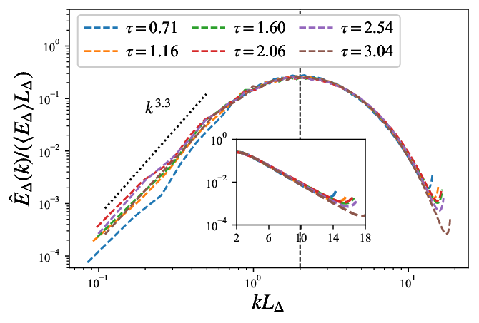
The uncertainty dissipation rate is the integral over all wavenumbers $k$ of $k^{2}\hat{E}_{\Delta}(k)$ where $\hat{E}_{\Delta}(k)$ is the uncertainty spectrum, i.e. the energy spectrum of the velocity difference field. The similarity in the evolutions of uncertainty production and dissipation rates raises the question whether the uncertainty spectrum evolves in some self-similar manner over the time range of that similarity. We answer this question in terms of the integral length scale of the velocity-difference fields considered here which is $L_{\Delta}=\left(3\pi/4\left\langle E_{\Delta}\right\rangle\right)\int k^{-1}\hat{E}_{\Delta}(k){\rm d}k$ (see Batchelor 1953 for an introduction to this length scale for any statistically homogeneous/periodic velocity field). $L_{\Delta}$ is a measure of the length over which the velocity difference field is correlated, i.e. a characteristic length scale of uncertainty containing eddies.

Soon after the initial decay of $\left\langle E_{\Delta}\right\rangle$, the uncertainty spectra collapse with $\left\langle E_{\Delta}\right\rangle(t)$ and $L_{\Delta}(t)$ at wavenumbers larger than $2/L_{\Delta}$ as shown in figure 4, i.e. $\hat{E}_{\Delta}(k,t)=\left\langle E_{\Delta}\right\rangle L_{\Delta}f(kL_{\Delta})$ for $kL_{\Delta}\geq 2$, where $f$ is a dimensionless function of dimensionless wavenumber. At wavenumbers $kL_{\Delta}<1$ the energy spectra have an approximately power law dependence on $k$ but do not collapse till soon after the time when the exponential growth of $\left\langle E_{\Delta}\right\rangle(t)$ and the uncertainty’s production-dissipation similarity ($\left\langle P_{\Delta}\right\rangle/\left\langle\varepsilon_{\Delta}\right\rangle\approx 1.6-1.7$) sets in. Over the time range when $\left\langle P_{\Delta}\right\rangle/\left\langle\varepsilon_{\Delta}\right\rangle\approx 1.6-1.7$, the uncertainty spectrum is self-similar, i.e. evolves as $\hat{E}_{\Delta}(k,t)=\left\langle E_{\Delta}\right\rangle L_{\Delta}f(kL_{\Delta})$ for all wavenumbers (see figure 5). The peak of the spectrum is at $k\approx 2/L_{\Delta}$ in all three cases F1, F2 and F3. At wavenumbers below $2/L_{\Delta}$ the uncertainty spectra have an approximately $k^{3.3}$ power law shape, while at wavenumbers above $2/L_{\Delta}$, they appear to have an exponential shape. Similar uncertainty spectrum shapes have been found in a previous DNS study (Berera & Ho 2018).

It is remarkable that the uncertainty spectrum is self-similar in case F3 in the exact same way that it is self-similar in cases F1 and F2 over the time range where $\left\langle P_{\Delta}\right\rangle/\left\langle\varepsilon_{\Delta}\right\rangle$ is approximately constant. In fact, the self-similar uncertainty spectrum even seems to be the same for F3, F1 and F2 as seen by the collapse in figure 5(d), suggesting a universal shape for the self-similar uncertainty spectrum in HIT. This is remarkable not only because $F3$ has a very different Reynolds number and forcing than F1 and F2, but more importantly because the F3 reference field is not statistically stationary in that time range whereas the F1 and F2 reference fields are. In the F3 case, the uncertainty spectrum reaches its self-similar state at $\tau\approx 5.8$ and the reference field becomes statistically stationary at $\tau=9.4$.

After the time-range where $\left\langle P_{\Delta}\right\rangle/\left\langle\varepsilon_{\Delta}\right\rangle$ is approximately constant, the uncertainty spectrum is no longer self-similar (see figure 6). This happens at $\tau=3.5$ for cases F1 and F2 and at $\tau=12.6$ for case F3 when $\hat{E}_{\Delta}(k_{max})/\hat{E}_{\text{tot}}(k_{max})>0.95$. These are the times when the reference and perturbed fields decorrelate at the largest resolvable wavenumber (see figure 6). The process of decorrelation between the two fields proceeds by decorrelating them at progressively smaller wavenumbers, causing the uncertainty spectrum to collapse with the reference field’s energy spectrum over a progressively wider range of the higher wavenumbers (see figure 6). This progressive decorrelation process from high to small wavenumbers and the uncertainty spectrum’s progressive convergence towards the reference field’s spectrum prevents the uncertainty spectrum from being self-similar. For F1, the uncertainty spectrum finally collapses with the reference field’s energy spectrum at all wavenumbers, indicating that the two fields eventually decorrelate completely at all wavenumbers (see figure 6(a)). The same happens for F2 and F3 except over the wavenumbers acted by the forcing where a gap always remains between the uncertainty and the reference field spectra, indicating that the two fields retain a degree of correlation at these large scales (see figure 6(b), 6(c)).

The growth of $L_{\Delta}$ is evident in figure 6. We therefore plot its time evolution in figure 7 and compare it with the integral and Taylor length scales ($L$ and $l_{\lambda}$ respectively) of the reference field for each case F1, F2 and F3. At the very early times when uncertainty dissipation dominates, the velocity-difference field decays and its integral length scale normalised by $L$ is, correspondingly, increasing. In the stationary turbulence F1 and F2 cases, this time regime is followed by the chaotic regime where $\left\langle E_{\Delta}\right\rangle$ grows exponentially and where $L_{\Delta}/l_{\lambda}^{(1)}$ remains relatively constant at $0.38\pm 0.01$. A constant $L_{\Delta}/l_{\lambda}^{(1)}$ (though a different constant, $L_{\Delta}/l_{\lambda}^{(1)}=0.64\pm 0.03$) is also observed in the non-stationary F3 case during the chaotic regime even though $l_{\lambda}^{(1)}$ grows in time for some of that regime and even though this time regime does not follow immediately after the dissipation-dominated regime. In fact, $L_{\Delta}$ decreases between the dissipation-dominated and the chaotic regime in the F3 case. It is noteworthy that $L_{\Delta}$ reaches $l_{\lambda}^{(1)}$ at $\tau=4.9$ for cases F1 and F2 and at $\tau=14.5$ for case F3, a little before the average uncertainty dissipation rate reaches its stationary value in figure 2, i.e. $\tau\approx 5.6$ for F1 and F2 and $\tau\approx 16.1$ for F3. The link between $L_{\Delta}$ and the Taylor length of the reference field is potentially interesting as the Taylor length is the mean distance between stagnation points in a homogeneous isotropic turbulence (Goto & Vassilicos 2009) and therefore tends to represent the average size of turbulent eddies which is highly weighted towards the more numerous smallest ones.

Following the exponential growth of $\left\langle E_{\Delta}\right\rangle$, three consecutive time regimes follow for F1 and F2. First, one observes an approximately power-law growth of $L_{\Delta}$, identical for both F1 and F2 as shown in figure 7(d), more or less coinciding with the exponential of exponential growth of $\left\langle E_{\Delta}\right\rangle$ till $\tau=6.5$. In this time regime, $L_{\Delta}\sim t^{3/2}$ is a good fit. This fit is reminiscent of the power-law growth of the predictability scale $k_{E}^{-1}\sim t^{3/2}$ obtained in previous numerical simulations (Boffetta & Musacchio 2017; Leith & Kraichnan 1972) and theoretical arguments (Boffetta & Musacchio 2017; Lorenz 1969; Frisch 1995), as a companion conclusion to the linear growth of $\left\langle E_{\Delta}\right\rangle$. However, $L_{\Delta}$ and $k_{E}^{-1}$ are not equivalent: the predictability scale is defined as the inverse of the minimum wavenumber $k_{E}$ such that $\hat{E_{\Delta}}(k_{E})/\hat{E}_{\text{tot}}(k_{E})=1$, and $k_{E}^{-1}\sim t^{3/2}$ is obtained on the assumption that the decorrelation process happens in the inertial range. $L_{\Delta}\sim t^{3/2}$ is observed without concurrent linear growth of $\left\langle E_{\Delta}\right\rangle$ but a concurrent exponential of exponential $\left\langle E_{\Delta}\right\rangle$ growth instead.

The second consecutive regime which follows for F1 and F2 is an apparently linear growth of $L_{\Delta}$ that lasts till the time when $L_{\Delta}$ saturates to a constant. The third and final regime is this approximately constant $L_{\Delta}$ regime where $L_{\Delta}\approx L^{(1)}$ for F1 (see figure 7(a)) in agreement with the eventual complete decorrelation of the reference and perturbed fields and where $L_{\Delta}\approx(0.70\pm 0.06)L^{(1)}$ (smaller than $L^{(1)}$) for F2 (see figure 7(b)) in agreement with the eventual partial correlation between these two fields in this case.

References

- Ashurst et al. (1987) Ashurst, W.T., Kerstein, A.R., Kerr, R.M. & Gibson, C.H. 1987 Alignment of vorticity and scalar gradient with strain rate in simulated Navier–Stokes turbulence. Phys. Fluids 30 (8), 2343–2353.
- Aurell et al. (1997) Aurell, E., Boffetta, G., Crisanti, A., Paladin, G. & Vulpiani, A. 1997 Predictability in the large: an extension of the concept of Lyapunov exponent. J. Phys. A Math. Theor. 30 (1), 1.
- Batchelor (1953) Batchelor, G. K. 1953 The theory of homogeneous turbulence. Cambridge university press.
- Berera & Ho (2018) Berera, A. & Ho, R.D.J.G. 2018 Chaotic properties of a turbulent isotropic fluid. Phys. Rev. Lett. 120 (2), 024101.
- Betchov (1956) Betchov, R. 1956 An inequality concerning the production of vorticity in isotropic turbulence. J. Fluid Mech. 1 (5), 497–504.
- Boffetta et al. (1997) Boffetta, G., Celani, A., Crisanti, A. & Vulpiani, A. 1997 Predictability in two-dimensional decaying turbulence. Phys. Fluids 9 (3), 724–734.
- Boffetta & Musacchio (2017) Boffetta, G. & Musacchio, S. 2017 Chaos and predictability of homogeneous-isotropic turbulence. Phys. Rev. Lett. 119 (5), 054102.
- Cheung & Wong (1987) Cheung, P.Y. & Wong, A.Y. 1987 Chaotic behavior and period doubling in plasmas. Phys. Rev. Lett. 59 (5), 551.
- Clark et al. (2021) Clark, D., Armua, A., Freeman, C., Brener, D.J. & Berera, A. 2021 Chaotic measure of the transition between two-and three-dimensional turbulence. Phys. Rev. Fluids 6 (5), 054612.
- Clark et al. (2022) Clark, D., Armua, A., Ho, R.D.J.G. & Berera, A. 2022 Critical transition to a non-chaotic regime in isotropic turbulence. J. Fluid Mech. 930.
- Crisanti et al. (1993) Crisanti, A., Jensen, M.H., Vulpiani, A. & Paladin, G. 1993 Intermittency and predictability in turbulence. Phys. Rev. Lett. 70 (2), 166.
- Deissler (1986) Deissler, R.G. 1986 Is Navier–Stokes turbulence chaotic? Phys. Fluids 29 (5), 1453–1457.
- Frisch (1995) Frisch, U. 1995 Turbulence: The Legacy of AN Kolmogorov. Cambridge University Press.
- Goto & Vassilicos (2009) Goto, S. & Vassilicos, J.C. 2009 The dissipation rate coefficient of turbulence is not universal and depends on the internal stagnation point structure. Phys. Fluids 21 (3), 035104.
- Ho et al. (2020) Ho, R.D.J.G., Armua, A. & Berera, A. 2020 Fluctuations of Lyapunov exponents in homogeneous and isotropic turbulence. Phys. Rev. Fluids 5 (2), 024602.
- Leith (1971) Leith, C.E. 1971 Atmospheric predictability and two-dimensional turbulence. J. Atmos. Sci. 28 (2), 145–161.
- Leith & Kraichnan (1972) Leith, C.E. & Kraichnan, R.H. 1972 Predictability of turbulent flows. J. Atmos. Sci. 29 (6), 1041–1058.
- Li (2014) Li, Y.C. 2014 The distinction of turbulence from chaos – rough dependence on initial data. Electron. J. Differ. Equ. 2014 (104), 1–8.
- Li et al. (2020) Li, Y.C., Ho, R.D.J.G., Berera, A. & Feng, Z.C. 2020 Superfast amplification and superfast nonlinear saturation of perturbations as a mechanism of turbulence. J. Fluid Mech. 904.
- Lorenz (1963) Lorenz, E.N. 1963 Deterministic nonperiodic flow. J. Atmos. Sci. 20 (2), 130–141.
- Lorenz (1969) Lorenz, E.N. 1969 The predictability of a flow which possesses many scales of motion. Tellus 21 (3), 289–307.
- Mohan et al. (2017) Mohan, P., Fitzsimmons, N. & Moser, R.D. 2017 Scaling of Lyapunov exponents in homogeneous isotropic turbulence. Phys. Rev. Fluids 2 (11), 114606.
- Paul et al. (2017) Paul, I., Papadakis, G. & Vassilicos, J. C. 2017 Genesis and evolution of velocity gradients in near-field spatially developing turbulence. J. Fluid Mech. 815, 295–332.
- Ruelle (1979) Ruelle, D. 1979 Microscopic fluctuations and turbulence. Phys. lett., A 72 (2), 81–82.
- Ruelle (1981) Ruelle, D. 1981 Small random perturbations of dynamical systems and the definition of attractors. Commun. Math. Phys. 82, 137–151.
- Sparrow (2012) Sparrow, C. 2012 The Lorenz equations: bifurcations, chaos, and strange attractors, , vol. 41. Springer Science & Business Media.
- Tennekes (1975) Tennekes, H 1975 Eulerian and Lagrangian time microscales in isotropic turbulence. J. Fluid Mech. 67 (3), 561–567.
- Tennekes & Lumley (1972) Tennekes, H. & Lumley, J.L. 1972 A first course in turbulence. MIT press.
- Vincent & Meneguzzi (1991) Vincent, A. & Meneguzzi, M. 1991 The spatial structure and statistical properties of homogeneous turbulence. J. Fluid Mech. 225, 1–20.
- Yoffe (2012) Yoffe, S.R. 2012 Investigation of the transfer and dissipation of energy in isotropic turbulence. PhD thesis, University of Edinburgh.