An efficient computational model of the in-flow capturing of magnetic nanoparticles by a cylindrical magnet for cancer nanomedicine
Barbara Wirthl1,*, Vitaly Wirthl2, Wolfgang A. Wall1
1 Institute for Computational Mechanics, Technical University of Munich, TUM School of Engineering and Design, Department of Engineering Physics & Computation, Garching b. München, Germany.
2 Max Planck Institute of Quantum Optics (MPQ), Garching b. München, Germany.
* B. Wirthl, E-mail: barbara.wirthl@tum.de
Abstract
Magnetic nanoparticles have emerged as a promising approach to improving cancer treatment. However, many novel nanoparticle designs fail in clinical trials due to a lack of understanding of how to overcome the in vivo transport barriers. To address this shortcoming, we develop a novel computational model aimed at the study of magnetic nanoparticles in vitro and in vivo. In this paper, we present an important building block for this overall goal, namely an efficient computational model of the in-flow capture of magnetic nanoparticles by a cylindrical permanent magnet in an idealised test setup. We use a continuum approach based on the Smoluchowski advection-diffusion equation, combined with a simple approach to consider the capture at an impenetrable boundary, and derive an analytical expression for the magnetic force of a cylindrical magnet of finite length on the nanoparticles. This provides a simple and numerically efficient way to study different magnet configurations and their influence on the nanoparticle distribution in three dimensions. Such an in silico model can increase insight into the underlying physics, help to design novel prototypes and serve as a precursor to more complex systems in vivo and in silico.
1 Introduction
Over the last three decades, nanoparticles have emerged as a promising approach to improve the effectiveness of cancer treatment because of their potential for sophisticated functionalisation and ability to accumulate in tumours [1]. Magnetic nanoparticles are of particular interest because of their ability to be controlled by an external magnetic field. To capture the drug-loaded magnetic nanoparticles in the target region, the applied magnetic force has to be strong enough to overcome fluid forces due to the blood flow or the interstitial fluid flow and further transport barriers, e.g., the extracellular matrix, the blood vessel wall, which the nanoparticles must cross, and different interfaces. However, this is often hard to achieve because of the inherently weak magnetic forces produced by an applied magnetic field—especially deeper in the body [2]. Because of those (and other) challenges, the design and successful application of magnetic nanoparticle-based cancer therapy is very demanding and almost hopeless purely via trial-and-error approaches in experimental research. Here, computational models can help by predicting the distribution of nanoparticles depending on the applied magnetic field and guide the design of novel prototypes.
On the way towards a comprehensive computational model of the capture of magnetic nanoparticles, we here start with an idealised test setup, illustrated in Fig. 1: a cylindrical permanent magnet is placed below a channel to capture the magnetic nanoparticles dispersed in the fluid flowing through the channel. This setup, even though simplified, contains the essential physics of the capture of magnetic nanoparticles: the magnetic force exerted by the magnet combined with the fluid flow, which is known to be a major transport barrier in vivo [3]. The bottom wall of the domain is impenetrable, so the captured nanoparticles accumulate at the wall. Such an idealised test setup, including tumour spheroids in the microfluidic channel, is used in experimental research, e.g., [4, 5, 6], because it allows insight into the fundamental physics of the capture of magnetic nanoparticles and serves as a precursor to more complex in vivo systems. The approaches and results of the current work are essential for exactly modelling the experimental setup where tumour spheroids are placed in the microfluidic channel [7].

To model the transport of magnetic nanoparticles, two approaches are the most common in the literature [8]: the first approach models the nanoparticles as discrete particles, while the second approach assumes that the nanoparticles behave as a continuum ferrofluid. The first approach considers the different forces acting on each particle individually, and Newton’s second law then describes the movement of each particle [9, 10, 11, 12]. This allows investigating the aggregation of the nanoparticles and the formation of particle clusters, e.g., chains [11, 12]. Nevertheless, when the system has a size of millimetres or centimetres, the number of particles in the domain is on the order of , which limits the applicability of this approach. Moreover, we are not interested in the movement of each particle individually. The second approach builds on the assumption that the nanoparticles have an infinitely strong coupling with the base fluid, and this fluid-particle mixture is described as a whole by the classical fluid equations, e.g., the Navier–Stokes equations [13, 14, 15, 16]. Hence, the magnetic force is part of the momentum balance equation. This approach, however, does not allow the nanoparticles to move relative to the fluid [16].
To overcome the limitations of both approaches, we take a different approach here, similar to [17]: we model the nanoparticles in a continuum sense, but consider that the nanoparticles can move relative to the advecting fluid due to diffusion and the exerted magnetic force. We therefore use an advection-diffusion equation to model the concentration of the nanoparticles and include the magnetic force directly in this equation. In this contribution, we address two specific challenges: the boundary condition at an impenetrable boundary and the efficient evaluation of the magnetic force exerted by a cylindrical magnet of finite length.
Concerning the first challenge (the boundary condition at an impenetrable boundary), [16] [16] state that most contributions in the literature that study the transport of magnetic nanoparticles in a continuum sense do not consider the boundary condition at the impenetrable boundary, which results in nanoparticles leaving the domain through the boundary. This however would be questionable for our long term goals, as we among others also want to be able to model complex time-dependent scenarios, where we should not loose nanoparticles. Hence, we present a simple approach to model the capture of magnetic nanoparticles at an impenetrable boundary.
Concerning the second challenge (the efficient evaluation of the magnetic force), we derive an analytical expression for the magnetic force on magnetic nanoparticles exerted by a cylindrical magnet of finite length. This presents a huge advantage of our approach, as it allows us to directly evaluate the magnetic force on the nanoparticles with minimal computational effort compared to numerically solving Maxwell’s equations. At the same time, we can study different magnet orientations in three dimensions—in contrast to two-dimensional models, commonly used in the literature [17, 18, 19, 20, 21, 2], which have the severe limitation that they assume the magnet to be infinitely long and oriented perpendicular to the two-dimensional domain.
In the following, we first introduce the equations for the advection-diffusion problem, including an impenetrable boundary, in Section 2.1. We then present the analytical expression for the magnetic force on the nanoparticles in Section 2.2. Section 3 presents and discusses numerical examples for both and Section 4 draws a conclusion.
2 Methods
2.1 Transport of nanoparticles: Smoluchowski advection-diffusion equation
We assume that the magnetic nanoparticles are dispersed in the fluid in a stable colloidal suspension, so the particle concentration is small (). We therefore assume that nanoparticles do not interact with each other, i.e., we neglect the inter-particle forces for now, and we assume that the nanoparticles do not influence the fluid flow.
The concentration of the nanoparticles is governed by the mass balance equation
| (1) |
where denotes the total flux. We here assume that neither sources nor sinks are present. The total flux is the sum of three contributions
| (2) |
arising from diffusion, advection and the magnetic force, respectively.
First, the diffusive flux arises from a local concentration gradient and is described by Fick’s first law
| (3) |
with the diffusion coefficient . Second, the advective flux arises from the velocity of the fluid advecting the nanoparticles and is given by
The fluid velocity might be given by solving the underlying flow problem, e.g., the Navier–Stokes equations or Darcy flow in a porous medium. For simplicity of presentations in this paper, we here directly prescribe the velocity of the fluid.
When the nanoparticles are not only subjected to fluid flow but additionally to a magnetic force, we include an additional magnetophoretic flux depending on the magnetic force . Typically, the resulting magnetophoretic velocity is assumed to be directly proportional to the applied force, e.g., see [22, 17], resulting in a magnetophoretic flux of
| (4) |
where is the mobility of a particle of radius in a fluid with dynamic viscosity11 1 denotes the dynamic viscosity of the fluid by the superscript (liquid) to distinguish it from the magnetic vacuum permeability introduced in Section 2.2. , based on Stokes’ law. Altogether, this results in the Smoluchowski advection-diffusion equation [23]
| (5) |
Eq. 4 assumes that the velocity is always directly proportional to the applied force. Now consider an example of a channel with an impenetrable wall and a force perpendicular to the wall, as sketched in Fig. 1: the force results in a velocity perpendicular to the wall, which in turn results in the nanoparticles leaving the domain through the impenetrable wall—which is obviously not physical.
We therefore introduce the mobility tensor , which relates the magnetophoretic velocity to the magnetic forces, i.e.,
| (6) |
or more explicitly,
| (7) |
similar to [24, 25]. The mobility is a tensor field that depends on the position . Now, a force in a specific direction does not necessarily result in a velocity in that direction, but only if the particle can move in this direction, i.e., if the mobility is non-zero. At an impenetrable wall, the nanoparticles cannot move in the direction perpendicular to the wall, i.e., into the wall, and thus the mobility is zero in this direction, resulting also in zero velocity. All off-diagonal entries of the mobility tensor are also zero: a force in one direction only causes a velocity in the same direction and no “shear” velocity. Inside the domain , which reduces back to Eq. 4. At the impenetrable wall (at ), the diagonal entries tangential to the wall still equal the scalar mobility, i.e., . However, the entry perpendicular to the wall is zero , as already mentioned above. The mobility tensor at the impenetrable wall is thus given by
| (8) |
The key point here is that we employ the mobility as a tensor field—as opposed to a scalar.
The final form of the Smoluchowski advection-diffusion equation is then given by
| (9) |
To solve this equation in space and time, we employ the standard Galerkin procedure to obtain the weak form of the equation and then discretise the equation in space using the finite element method (FEM) and in time using the backward Euler method. We use our in-house parallel multiphysics research code BACI [26] as a computational framework.
Remark (Stabilisation).
In our case, Eq. 9 is dominated by the two convective terms, which causes numerical instabilities when using the standard Galerkin procedure. We therefore use the streamline upwind Petrov–Galerkin (SUPG) method [27] to stabilise the equation, where numerical diffusion along streamlines is introduced in a consistent manner [28]. We choose the stabilisation parameter based on [29] [29].
2.2 Magnetic force on the nanoparticles
Due to the permanent magnet, the magnetic nanoparticles are subjected to a static non-homogenous external magnetic field leading to a force . This force however does not only depend on the magnetic field but also the magnetic response of the particles.
Due to the small size of the particles, we assume that they can be modelled as an equivalent point dipole located at the centre of the particle (effective dipole moment approach [30, 8, 17]). Also, due to the small size, the nanoparticles are superparamagnetic: they are magnetised with a large magnetic susceptibility when an external magnetic field is applied but do not retain their magnetisation after the external magnetic field is removed. Hence, when a superparamagnetic nanoparticle is placed in an external magnetic field, it magnetises, resulting in a magnetic moment . The force on the magnetic dipole induced in the nanoparticle is then given by
| (10) |
with the magnetic vacuum permeability 22 2 We assume that the fluid (water) and air are non-magnetic, and thus assume that their permeability is equal to the vacuum magnetic permeability defined as [31]. The exact values for water and air differ from the value for vacuum at the fifth and seventh decimal place, respectively. . Using the magnetisation as the magnetic moment per volume, i.e., with being the volume of the nanoparticle, the force can be written as
| (11) |
Thus, the force depends on the magnetisation of the nanoparticle and the derivatives of the applied magnetic field.
The magnetised nanoparticles also produce a magnetic field, affecting the nearby nanoparticles. For now, we assume that the magnetic force that the nanoparticles exert on each other is negligible compared to the magnetic force exerted by the external magnetic field—which is a valid assumption for low concentrations of nanoparticles and hence large distances between the nanoparticles [16, 32, 33, 17, 34]. We will investigate and discuss the validity of this assumption in Section 3.3.
Magnetisation model
To relate the magnetisation of the nanoparticle to the applied magnetic field, we use a linear magnetisation model with saturation, given by
| (12) |
with being the saturation magnetisation and the field strength for which the particle reaches saturation, as presented by [17, 8, 22]. An example of such a magnetisation curve is shown in Fig. 2. If the particle is below saturation, its magnetisation is proportional to the applied magnetic field
| (13) |
and the particle reaches saturation for
| (14) |
which can be derived based on the effective dipole moment approach [30, 17]. Above saturation, the magnetisation is equal to the saturation magnetisation
| (15) |
The magnetisation is always aligned with the applied magnetic field.
Finally, as discussed above, the particles are superparamagnetic: their magnetic susceptibility is much higher than the magnetic susceptibility of paramagnetic materials, i.e., [17, 35, 36]. Eq. 12 can then be simplified to
| (16) |
In sum, the magnetic force on the nanoparticles is given by
| (17) |
which shows that the magnetic force depends both on the strength of the magnetic field and its derivatives.
Analytical expression for the magnetic field
Usually, the magnetic field is obtained by solving Maxwell’s equations numerically. Analytic expressions are only well-known for some classic textbook cases: the magnetic field of point multipoles and infinitely long wires carrying a current [37]. However, for a finite-length cylindrical magnet, which we have here, [38] [38] and [39] [39] presented analytic expressions based on the elliptic integrals. These analytic expressions are beneficial because the magnetic quantities can be evaluated at all coordinates with minimal computational effort compared to numerically solving Maxwell’s equations, e.g., using the FEM.
In the following, we summarise the analytic expression for the magnetic field, as presented by [38, 39], and then extend this by deriving the analytic expressions for the magnetic force. The cylindrical magnet is magnetised in the longitudinal direction. The field components of the magnetic field in cylindrical coordinates are given by
| (18) | ||||
| (19) |
and due to the radial symmetry of the system [38, 39]33 3 Eqs. 18 and 19 are mathematically well-behaved except on the edge of the magnet at and [38].. Here, denotes the magnetisation of the cylindrical magnet and its radius. The origin of the cylindrical coordinate system is located at the centre of the magnet. The two auxiliary functions and are defined as
| (20) | ||||
| (21) |
with the following auxiliary variables
and being the length of the cylindrical magnet. Eqs. 20 and 21 are based on the complete elliptic integrals of the first, second and third kind, which in Legendre’s notation are written as
| (22) | ||||
| (23) | ||||
| (24) |
All three kinds of elliptic integrals can be efficiently evaluated using Carlson’s functions , and [40, 41] as
| (25) | ||||
| (26) | ||||
| (27) |
Numerical Recipies [42] provides algorithms and source code for evaluating Carlson’s functions, which are also implemented in Mathematica [43] and SciPy [44].
Remark (Parameter and sign conventions in the elliptic integrals).
Note that Numerical Recipies [42, p. 315] uses a different sign convention for the variable in the third elliptic integral, such that
| (28) |
Additionally, [39] use the convention with parameter , where in their Eq. (6) in [39]. Mathematica [43] and SciPy [44] however use the parameter , as presented here in Eqs. 22, 23 and 24.
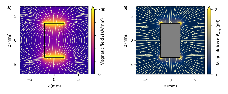
Fig. 3A shows an example of the magnetic field of a cylindrical magnet with radius , length and magnetisation . Inside the magnet, the magnetic field is given by , with the magnetic flux density . For a longitudinally magnetised magnet, the magnetisation vector is , with being the unit vector in -direction. The magnetisation vector is constant inside and zero outside the magnet. The result for the magnetic field in Fig. 3A is qualitatively well known: the magnetic field lines start at one pole and end at the other, forming fanned-out circular segments around the magnet.
Analytical expression for the magnetic force
As discussed above, the magnetic force depends on the magnetic field and its derivatives. Since the first derivatives of the elliptic integrals are known analytically, we can derive an analytical expression for the magnetic force . Evaluating Eq. 17 for the analytical expression for the magnetic field results in the force components given by
| (29) |
and
| (30) |
with two auxiliary functions and based on the elliptic integrals
and the following auxiliary variables44 4 Note that Eqs. 29 and 30 are undefined at and . Outside the magnet, these singularities are removable and is extendable.
The coordinate transformations from cylindrical coordinates to cartesian coordinates are given by
| (31) | ||||
| (32) | ||||
| (33) |
with and 55 5 Most programming languages provide a function arctan2(y,x) which is defined for all and returns the correct angle with respect to the quadrant of the point ..
Fig. 3B shows the magnetic force for a cylindrical magnet with radius and length . Calculating the magnetic force is only meaningful outside the magnet. The magnetic force is on the order of , similar to the order of magnitude estimated in [12] for a similar configuration.
We also provide a Python implementation of the analytical expressions for the magnetic field and force [45].
3 Numerical examples and discussion
In the following, we present and discuss numerical examples to demonstrate the capabilities of the proposed model. In Section 3.1, we start with a two-dimensional example where we investigate the influence of the mobility tensor field on the nanoparticle capture at the impenetrable wall. Next, in Section 3.2, we investigate the nanoparticle distribution in three dimensions for different positions and orientations of a finite-length cylindrical magnet, leveraging the analytic expression for the magnetic force, which we derived. Finally, in Section 3.3, using the analytical expressions for the magnetic field and force, we examine the validity of the assumption that the inter-particle forces are negligible compared to the magnetic force exerted by the external magnetic field.
3.1 Influence of the mobility tensor field
We first present a two-dimensional example where we investigate the influence of the mobility tensor field on the distribution of the magnetic particles.
The computational setup is depicted in Fig. 4A. We study a two-dimensional slice in the XZ-plane with a size of , which is discretised with linear rectangular elements. The time step size is and the total simulation time is . For simplicity, we consider a constant advective flow velocity along the -axis and a constant magnetic force along the -axis, which is a reasonable order of magnitude for the considered cylindrical magnets (see Fig. 3B). For a water-like fluid with a viscosity of and nanoparticles with a radius of , this corresponds to a magnetophoretic velocity of . We assume a diffusion coefficient of . On the inflow boundary at , we prescribe the concentration of nanoparticles as a Dirichlet boundary condition given by a bell-shaped function with a maximum value of .

The wall at the bottom of the domain is impenetrable, and we prescribe a Dirichlet boundary condition for the concentration of nanoparticles given by . Additionally, the z-component of the mobility tensor field is zero at the bottom wall, i.e., . We compare the results for the nanoparticle distribution given different functions for , as given in Fig. 4B. On the one hand, we consider the Heaviside function , with being the boundary layer thickness: this means that the mobility of the nanoparticles is zero in the boundary layer. We choose so that the boundary layer is two or three elements wide (given an element size of ). On the other hand, we consider different smooth functions for , which have the value one inside the domain and have different slopes towards the boundary.
Fig. 4C presents the results given the different functions for . In all cases, the nanoparticles accumulate at the impenetrable wall at the bottom of the domain, which was the primary motivation for introducing the mobility tensor field. All functions lead to a similar distribution of the nanoparticles, with the thickness of the layer of captured nanoparticles depending on the function . However, it shall be noted that the smooth functions are—as to be expected—numerically better behaved than the Heaviside function, which can cause convergence issues.
Defining a tensor field is a simple way to model the accumulation of nanoparticles at an impenetrable wall. It is worth noting that most similar studies in the literature, e.g., [17, 18, 46], do not clarify and also seem to not use appropriate boundary conditions for the nanoparticles at the wall. This allows for studying the trajectories of the nanoparticles in the bulk of the fluid, but it is impossible to investigate the capture of the nanoparticles at a wall. Only [16] [16] presented and discussed an approach for an impermeability condition at the wall: they set the combined advective-diffusive flux to zero
| (34) |
We drop the advective velocity because any physically plausible velocity field cannot have a component perpendicular to an impermeable wall, either by directly imposing a physically plausible velocity field (as we do here) or by prescribing a no-slip boundary condition and solving the fluid equations. [16] [16] subsequently set the normal component of the magnetophoretic velocity at the wall also to zero. Eq. 34 then reduces to the classical Neumann boundary condition , which we also impose. In sum, their boundary condition is equivalent to our approach based on setting the normal component of the mobility tensor to zero, i.e., .
Nevertheless, [16] [16] also stated that their employed boundary condition poses a numerical challenge due to the steep concentration gradient at the wall. They solve this problem by prior grid refinement adaptive to the magnetic field gradient. We circumvent this problem by setting the mobility to zero on several elements or by using a smooth function.
3.2 Nanoparticle capture with a cylindrical magnet of finite length
We now investigate a three-dimensional example with a cylindrical magnet positioned below the fluid domain. The analytical solution for the magnetic force enables us to efficiently compare different orientations of a cylindrical magnet.
The computational setup is the one sketched in Fig. 1. The domain has a size of , which is discretised with linear hexahedral elements. The time step size is again and the total simulated time . For simplicity, we also again assume a constant advective flow velocity of . The parameters for the magnetic nanoparticles, the magnet, and the fluid are given in Table 1. The nanoparticle concentration on the inflow boundary is again defined by and zero at the bottom wall. We use a smooth function for the mobility tensor field, i.e., Function 4 shown in Fig. 4B and discussed in the previous subsection.
| Symbol | Parameter | Value | Units | Ref. |
| Magnetic nanoparticles | ||||
| Radius of the nanoparticles | [17] | |||
| Diffusion coefficient | Assumed | |||
| Saturation magnetisation | [17] | |||
| Magnet | ||||
| Radius of the magnet | Assumed | |||
| Length of the magnet | Assumed | |||
| Magnetisation of the magnet | [17] | |||
| Fluid (water) | ||||
| Dynamic viscosity | Known | |||
The cylindrical magnet has a radius of and a length of and is centered below the domain with a distance of to the bottom wall. In the first step, we compare three different orientations of the magnet: A) The magnet is oriented vertically (along the z-axis); B) The magnet is oriented horizontally (along the x-axis); C) The magnet is rotated around the y-axis.
Fig. 5 shows the concentration of the nanoparticles for the three different orientations of the magnet. For the vertical orientation, the nanoparticles are attracted to the magnet and accumulate at the bottom wall in a circular shape directly above the magnet, similar to experimental results, e.g., [6]. For the horizontal orientation, the nanoparticles accumulate above the two ends of the magnet, forming two ellipses. For the orientation, the nanoparticles form one ellipse above where the edge of the magnet is closest to the bottom wall.

Examples in the literature are restricted to a single orientation of a cylindrical magnet of infinite length, e.g., [17, 2]. In particular, we show that the nanoparticles accumulate above the ends of the magnet—which can obviously not be investigated with a magnet of infinite length.
Further, we here leverage what [38] [38] and [39] [39] stated: their derived analytical expressions for the magnetic field of magnetised cylinders are especially convenient for applications where magnetic forces on magnetic dipoles are required—nanoparticles being one such example. Nevertheless, our results for the magnetic force are restricted to a cylindrical magnet of finite length with longitudinal magnetisation. Similar analytical solutions for cylindrical magnets with arbitrary magnetisation can also be derived based on the respective analytical expressions for the magnetic field presented by [39] [39]. However, if the magnet is of an arbitrary shape, the magnetic field and force must be evaluated based on numerically solving Maxwell’s equations.
Several studies in the literature, e.g., [17, 18, 19, 20, 21, 2] reduced the setup to a two-dimensional problem in the XZ-plane and assumed the cylindrical magnet to be infinitely long. In this case, the magnetic force can also be expressed analytically, as derived in [17], and given by
| (35) | ||||
| (36) |
where the coordinate system is at the centre of the magnet, and the longitudinal axis of the magnet is perpendicular to the XZ-plane. We now compare results based on this assumption of an infinitely long magnet to the results for a finite-length magnet, as derived in this contribution. In both cases, we assume that the magnet has a radius of and a distance of to the bottom boundary of the domain. The cylindrical magnet of finite length has a length of , as used in the previous examples. For simplicity, we here assume that in both cases.
Fig. 6 shows the magnetic force and the resulting nanoparticle distribution for the magnet of infinite length compared to the finite-length magnet. As is also evident in Fig. 3, the magnetic force of the finite-length magnet varies along the longitudinal axis of the magnet, and so we compare the force in different slices along the longitudinal axis, in this case the -axis (but the -axis in Fig. 3). As evident in Fig. 6, the direction of the magnetic force is the same in all cases, but the magnitude is significantly different. For the cylindrical magnet of infinite length, the maximum force in the domain is . For the finite-length magnet, the maximum force varies considerably depending on the position of the slice: the maximum magnitude is , , and for the slices at , , and , respectively. Accordingly, the nanoparticle distributions are also markedly different: the nanoparticles accumulate in a higher concentration above the ends of the finite-length magnet than along the infinitely long magnet.

In sum, one has to be aware that the assumption of an infinitely long magnet leads to significantly different results than a finite-length magnet. The analytical solution for the finite-length magnet—as derived in this contribution—provides a simple and computationally efficient way to investigate the transport of nanoparticles in a more realistic setup.
3.3 Comparison of the force exerted by the permanent magnet to the inter-particle forces
In this contribution, we only consider the external magnetic force the permanent magnet exerts on the nanoparticles. However, the nanoparticles also exert forces on each other, and thus the question arises when these inter-particle forces are negligible compared to the force exerted by the permanent magnet. So far in this contribution, we have assumed that the low concentration of nanoparticles ensures that the inter-particle distance is large enough for the inter-particle forces to be negligible, similar to [16, 32, 33, 17, 34].
In general, the cut-off length of dipole-dipole interactions in nanoparticle assemblies is about three particle diameters [47]. Assuming that the nanoparticles are more than three particle diameters apart seems reasonable for the nanoparticles dissolved in the flowing fluid in our previous examples. However, when the nanoparticles accumulate at the bottom of the domain, they come very close to each other, and thus the inter-particle forces might become relevant there.
Therefore, we compare the external magnetic force to the inter-particle forces. We use our analytical expressions for the magnetic field and the external magnetic force and build on the force comparison presented by [12] [12], who investigated a similar setup. We analyse a simplified example shown in Fig. 7A: we consider two nanoparticles with a diameter of and a distance between their centres. The cylindrical magnet is positioned vertically below the domain (see previous example Fig. 5A). We assume that the two nanoparticles are aligned with the magnetic field such that is parallel to . We again assume for simplicity.

In the following, the non-bold symbols denote the magnitudes of the vectors, e.g., , and a hat denotes the unit vector in the given direction, e.g., .
As discussed in Section 2.2, the nanoparticles are modelled as point dipoles, with the magnetic moment of nanoparticle given by
| (37) |
Thus, the magnetic moment of the nanoparticle is aligned with the applied magnetic field. Since the nanoparticles are much smaller than the computational domain, we assume that and hence . The magnetised nanoparticle generates a magnetic field at the position of nanoparticle given by [37] as
| (38) |
In our case, and Eq. 38 simplifies to
| (39) |
Hence, the total magnetic field at the position of nanoparticle is given by
| (40) |
and accordingly, the magnetic moment of nanoparticle also changes to
| (41) |
The magnetic moments of both particles increase due to the cross-effects. The new values for the magnetic moments can be substituted back into the previous equations to calculate a second correction of the magnetic field and magnetic moments. In practice, this is not necessary, and we omit it [33, 12].
The force between the two particles, i.e., the inter-particle force, is given by [48] as
| (42) |
We evaluate the inter-particle force for different distances between the two nanoparticles: . Fig. 7B shows the force exerted by the external magnet and Fig. 7C the inter-particle force . For a distance of five particle diameters, the forces are on the same order of magnitude, namely . However, the inter-particle force strongly increases for smaller distances: for a distance of one particle diameter, it is about three orders of magnitude larger than the force of the external magnet, especially for the particles at the bottom of the domain. This is in good agreement with the results of [12] [12].
These results underline that one cannot simply assume that the inter-particle forces are negligible but must carefully assess whether they are relevant in the configuration studied with the assumptions made.
4 Conclusion
In this contribution, we presented a continuum approach based on the Smoluchowski advection-diffusion equation to model the capture of magnetic nanoparticles under the combined effect of fluid flow and magnetic forces. We included a simple and numerically stable way to consider an impenetrable boundary where the nanoparticles are captured. Further, the analytical expression for the magnetic force of a cylindrical magnet of finite length on the magnetic nanoparticles, which we derived, provides an efficient way to model the capture of magnetic nanoparticles in a more realistic setup in three dimensions.
Since many novel nanoparticle designs fail in clinical trials, our modelling efforts can help to gain insight into the behaviour of magnetic nanoparticles and help to design novel prototypes. While our expression for the magnetic force is restricted to cylindrical magnets, this is the configuration that is commonly used in experiments, e.g., when studying magnetic nanoparticles in fluidic devices [4, 5, 6]. Hence, such an in silco model can help with experimental design to limit the number of experiments and thus the costs to the most promising configurations. Finally, the presented model can serve as a precursor to more complex models, e.g., including magnets of arbitrary shape or considering complex biomechanical models coupling the transport of the nanoparticles in the blood vessels with the crossing of the vessel walls and the accumulation in the tumour tissue—both in vivo and in silico [49, 50, 7].
Acknowledgements
WAW was supported by BREATHE, a Horizon 2020|ERC-2020-ADG project, grant agreement No. 101021526-BREATHE.
References
- 1. Jinjun Shi, Philip. Kantoff, Richard Wooster and Omid. Farokhzad “Cancer nanomedicine: progress, challenges and opportunities” In Nature Reviews Cancer 17.1 Nature Publishing Group, 2017, pp. 20–37 DOI: 10.1038/nrc.2016.108
- 2. Rodward. Hewlin and Joseph. Tindall “Computational Assessment of Magnetic Nanoparticle Targeting Efficiency in a Simplified Circle of Willis Arterial Model” In International Journal of Molecular Sciences 24.3 Multidisciplinary Digital Publishing Institute, 2023, pp. 2545 DOI: 10.3390/ijms24032545
- 3. Namid. Stillman, Marina Kovacevic, Igor Balaz and Sabine Hauert “In Silico Modelling of Cancer Nanomedicine, across Scales and Transport Barriers” In npj Computational Materials 6.1 Nature Publishing Group, 2020, pp. 1–10 DOI: 10.1038/s41524-020-00366-8
- 4. K. Nguyen, B. Nu, M. M\"uhlberger, H. Unterweger, R.P. Friedrich, C. Alexiou and C. Janko “Superparamagnetic Iron Oxide Nanoparticles Carrying Chemotherapeutics Improve Drug Efficacy in Monolayer and Spheroid Cell Culture by Enabling Active Accumulation” In Nanomaterials 10.8, 2020, pp. 1–21 DOI: 10.3390/nano10081577
- 5. Jessica Behr, Lucas. Carnell, Rene Stein, Felix Pfister, Bernhard Friedrich, Christian Huber, Stefan Lyer, Julia Band, Eveline Schreiber, Christoph Alexiou and Christina Janko “In Vitro Setup for Determination of Nanoparticle-Mediated Magnetic Cell and Drug Accumulation in Tumor Spheroids under Flow Conditions” In Cancers 14.23 Multidisciplinary Digital Publishing Institute, 2022, pp. 5978 DOI: 10.3390/cancers14235978
- 6. Mona Kappes, Bernhard Friedrich, Felix Pfister, Christian Huber, Ralf Friedrich, Ren\’e Stein, Christian Braun, Julia Band, Eveline Schreiber, Christoph Alexiou and Christina Janko “Superparamagnetic Iron Oxide Nanoparticles for Targeted Cell Seeding: Magnetic Patterning and Magnetic 3D Cell Culture” In Advanced Functional Materials, 2022, pp. 2203672 DOI: 10.1002/adfm.202203672
- 7. Barbara Wirthl, Christina Janko, Stefan Lyer, Bernhard Schrefler, Christoph Alexiou and Wolfgang Wall “An in silico model of the capturing of magnetic nanoparticles in tumour spheroids in the presence of flow” Submitted, 2023
- 8. Bart Hallmark, Nicholas. Darton and Daniel Pearce “Modeling the In-Flow Capture of Magnetic Nanoparticles” In Magnetic Nanoparticles in Biosensing and Medicine Cambridge, UK: Cambridge University Press, 2019, pp. 151–171 DOI: 10.1017/9781139381222.006
- 9. P.. Cregg, Kieran Murphy and Adil Mardinoglu “Inclusion of Magnetic Dipole–Dipole and Hydrodynamic Interactions in Implant-Assisted Magnetic Drug Targeting” In Journal of Magnetism and Magnetic Materials 321.23, 2009, pp. 3893–3898 DOI: 10.1016/j.jmmm.2009.07.056
- 10. P.. Cregg, Kieran Murphy, Adil Mardinoglu and Adriele Prina-Mello “Many Particle Magnetic Dipole–Dipole and Hydrodynamic Interactions in Magnetizable Stent Assisted Magnetic Drug Targeting” In Journal of Magnetism and Magnetic Materials 322.15, 2010, pp. 2087–2094 DOI: 10.1016/j.jmmm.2010.01.038
- 11. P\’eter P\’alovics, M\’arton N\’emeth and M\’arta Rencz “Investigation and Modeling of the Magnetic Nanoparticle Aggregation with a Two-Phase CFD Model” In Energies 13.18 Multidisciplinary Digital Publishing Institute, 2020, pp. 4871 DOI: 10.3390/en13184871
- 12. P\’eter P\’alovics and M\’arta Rencz “Investigation of the Motion of Magnetic Nanoparticles in Microfluidics with a Micro Domain Model” In Microsystem Technologies 28.6, 2022, pp. 1545–1559 DOI: 10.1007/s00542-020-05077-0
- 13. X.. Li, K.. Yao, H.. Liu and Z.. Liu “The Investigation of Capture Behaviors of Different Shape Magnetic Sources in the High-Gradient Magnetic Field” In Journal of Magnetism and Magnetic Materials 311.2, 2007, pp. 481–488 DOI: 10.1016/j.jmmm.2006.07.040
- 14. X.. Li, K.. Yao and Z.. Liu “CFD Study on the Magnetic Fluid Delivering in the Vessel in High-Gradient Magnetic Field” In Journal of Magnetism and Magnetic Materials 320.11, 2008, pp. 1753–1758 DOI: 10.1016/j.jmmm.2008.01.041
- 15. A. Munir, J. Wang and H.. Zhou “Dynamics of Capturing Process of Multiple Magnetic Nanoparticles in a Flow through Microfluidic Bioseparation System” In IET Nanobiotechnology 3.3 IET Digital Library, 2009, pp. 55–64 DOI: 10.1049/iet-nbt.2008.0015
- 16. Saud. Khashan, Emad Elnajjar and Yousef Haik “CFD Simulation of the Magnetophoretic Separation in a Microchannel” In Journal of Magnetism and Magnetic Materials 323.23, 2011, pp. 2960–2967 DOI: 10.1016/j.jmmm.2011.06.001
- 17. E.. Furlani and K.. Ng “Analytical Model of Magnetic Nanoparticle Transport and Capture in the Microvasculature” In Physical Review E 73.6 American Physical Society, 2006, pp. 061919 DOI: 10.1103/PhysRevE.73.061919
- 18. Edward. Furlani and Edward. Furlani “A Model for Predicting Magnetic Targeting of Multifunctional Particles in the Microvasculature” In Journal of Magnetism and Magnetic Materials 312.1, 2007, pp. 187–193 DOI: 10.1016/j.jmmm.2006.09.026
- 19. Lioz Etgar, Arie Nakhmani, Allen Tannenbaum, Efrat Lifshitz and Rina Tannenbaum “Trajectory Control of PbSe–-Fe2O3 Nanoplatforms under Viscous Flow and an External Magnetic Field” In Nanotechnology 21.17, 2010, pp. 175702 DOI: 10.1088/0957-4484/21/17/175702
- 20. Sachin Shaw “Mathematical Model on Magnetic Drug Targeting in Microvessel” In Magnetism and Magnetic Materials IntechOpen, 2018 DOI: 10.5772/intechopen.73678
- 21. E.. Yeo, H. Markides, A.. Schade, A.. Studd, J.. Oliver, S.. Waters and A.. El “Experimental and Mathematical Modelling of Magnetically Labelled Mesenchymal Stromal Cell Delivery” In Journal of The Royal Society Interface 18.175 Royal Society, 2021, pp. 20200558 DOI: 10.1098/rsif.2020.0558
- 22. M. Takayasu, R. Gerber and F. Friedlaender “Magnetic Separation of Submicron Particles” In IEEE Transactions on Magnetics 19.5, 1983, pp. 2112–2114 DOI: 10.1109/TMAG.1983.1062681
- 23. M.V. Smoluchowski “Über Brownsche Molekularbewegung Unter Einwirkung Äußerer Kräfte Und Deren Zusammenhang Mit Der Verallgemeinerten Diffusionsgleichung” In Annalen der Physik 4.48, 1915, pp. 1103–1112 DOI: 10.1002/andp.19163532408
- 24. D. Pimponi, M. Chinappi, P. Gualtieri and C.. Casciola “Mobility Tensor of a Sphere Moving on a Superhydrophobic Wall: Application to Particle Separation” In Microfluidics and Nanofluidics 16.3, 2014, pp. 571–585 DOI: 10.1007/s10404-013-1243-4
- 25. Kongtao Chen, Jian Han, Xiaoqing Pan and David. Srolovitz “The Grain Boundary Mobility Tensor” In Proceedings of the National Academy of Sciences 117.9 Proceedings of the National Academy of Sciences, 2020, pp. 4533–4538 DOI: 10.1073/pnas.1920504117
- 26. BACI “A Comprehensive Multi-Physics Simulation Framework.” Accessed: 06.09.2023, 2023 URL: https://baci.pages.gitlab.lrz.de/website/
- 27. Alexander. Brooks and Thomas J.. Hughes “Streamline Upwind/Petrov-Galerkin Formulations for Convection Dominated Flows with Particular Emphasis on the Incompressible Navier-Stokes Equations” In Computer Methods in Applied Mechanics and Engineering 32.1, 1982, pp. 199–259 DOI: 10.1016/0045-7825(82)90071-8
- 28. Volker John and Petr Knobloch “On Discontinuity—Capturing Methods for Convection—Diffusion Equations” In Numerical Mathematics and Advanced Applications Berlin, Heidelberg: Springer, 2006, pp. 336–344 DOI: 10.1007/978-3-540-34288-5_27
- 29. Ramon Codina “Stabilized Finite Element Approximation of Transient Incompressible Flows Using Orthogonal Subscales” In Computer Methods in Applied Mechanics and Engineering 191.39, 2002, pp. 4295–4321 DOI: 10.1016/S0045-7825(02)00337-7
- 30. Thomas. Jones “Fundamentals” In Electromechanics of Particles Cambridge, UK: Cambridge University Press, 1995, pp. 5–33 DOI: 10.1017/CBO9780511574498.004
- 31. Eite Tiesinga, Peter. Mohr, David. Newell and Barry. Taylor “CODATA Recommended Values of the Fundamental Physical Constants: 2018” In Reviews of Modern Physics 93.2 American Physical Society, 2021, pp. 025010 DOI: 10.1103/RevModPhys.93.025010
- 32. Eric. Keaveny and Martin. Maxey “Modeling the Magnetic Interactions between Paramagnetic Beads in Magnetorheological Fluids” In Journal of Computational Physics 227.22, 2008, pp. 9554–9571 DOI: 10.1016/j.jcp.2008.07.008
- 33. K. Han, Y.. Feng and D… Owen “Three-Dimensional Modelling and Simulation of Magnetorheological Fluids” In International Journal for Numerical Methods in Engineering 84.11, 2010, pp. 1273–1302 DOI: 10.1002/nme.2940
- 34. Magdalena Woi\’nska, Jacek Szczytko, Andrzej Majhofer, Jacek Gosk, Konrad Dziatkowski and Andrzej Twardowski “Magnetic Interactions in an Ensemble of Cubic Nanoparticles: A Monte Carlo Study” In Physical Review B 88.14 American Physical Society, 2013, pp. 144421 DOI: 10.1103/PhysRevB.88.144421
- 35. Conroy Sun, Jerry S.. Lee and Miqin Zhang “Magnetic Nanoparticles in MR Imaging and Drug Delivery” In Advanced Drug Delivery Reviews 60.11, Inorganic Nanoparticles in Drug Delivery, 2008, pp. 1252–1265 DOI: 10.1016/j.addr.2008.03.018
- 36. Karrina McNamara and Syed A.. Tofail “Nanoparticles in Biomedical Applications” In Advances in Physics: X 2.1 Taylor & Francis, 2017, pp. 54–88 DOI: 10.1080/23746149.2016.1254570
- 37. John Jackson “Classical Electrodynamics: International Adaptation” Hoboken, NY: Wiley, 2021
- 38. Norman Derby and Stanislaw Olbert “Cylindrical Magnets and Ideal Solenoids” In American Journal of Physics 78.3 American Association of Physics TeachersAAPT, 2010, pp. 229 DOI: 10.1119/1.3256157
- 39. Alessio Caciagli, Roel. Baars, Albert. Philipse and Bonny W.. Kuipers “Exact Expression for the Magnetic Field of a Finite Cylinder with Arbitrary Uniform Magnetization” In Journal of Magnetism and Magnetic Materials 456, 2018, pp. 423–432 DOI: 10.1016/j.jmmm.2018.02.003
- 40. B.. Carlson “Computing Elliptic Integrals by Duplication” In Numerische Mathematik 33.1, 1979, pp. 1–16 DOI: 10.1007/BF01396491
- 41. B.. Carlson and Elaine. Notis “Algorithms for Incomplete Elliptic Integrals” In ACM Transactions on Mathematical Software 7.3, 1981, pp. 398–403 DOI: 10.1145/355958.355970
- 42. William. Press, Saul. Teukolsky, William. Vetterling and Brian. Flannery “Numerical Recipes 3rd Edition: The Art of Scientific Computing” Cambridge, UK: Cambridge University Press, 2007 URL: http://numerical.recipes/
- 43. Wolfram Research, Inc. “Mathematica, Version 13.3”, 2023 URL: https://www.wolfram.com/mathematica/
- 44. Pauli Virtanen et al. “SciPy 1.0: Fundamental Algorithms for Scientific Computing in Python” In Nature Methods 17.3 Nature Publishing Group, 2020, pp. 261–272 DOI: 10.1038/s41592-019-0686-2
- 45. Barbara Wirthl “Implementation of the Analytical Expressions for the Magnetic Field and Force of Finite-Length Cylindrical Permanent Magnet” In GitHub, 2023 URL: https://github.com/bwirthl/cylindrical-magnet-functions
- 46. Laura\’ra Roa-Barrantes and Diego\’an Rodriguez “Magnetic Field Effect on the Magnetic Nanoparticles Trajectories in Pulsating Blood Flow: A Computational Model” In BioNanoScience 12.2, 2022, pp. 571–581 DOI: 10.1007/s12668-022-00949-3
- 47. Gabriele Barrera, Paolo Allia and Paola Tiberto “Dipolar Interactions among Magnetite Nanoparticles for Magnetic Hyperthermia: A Rate-Equation Approach” In Nanoscale 13.7 The Royal Society of Chemistry, 2021, pp. 4103–4121 DOI: 10.1039/D0NR07397K
- 48. David. Griffiths “Introduction to Electrodynamics” Cambridge, UK: Cambridge University Press, 2017 DOI: 10.1017/9781108333511
- 49. Johannes Kremheller, Anh-Tu Vuong, Bernhard. Schrefler and Wolfgang. Wall “An approach for vascular tumor growth based on a hybrid embedded/homogenized treatment of the vasculature within a multiphase porous medium model” In International Journal for Numerical Methods in Biomedical Engineering 35.11, 2019, pp. e3253 DOI: 10.1002/cnm.3253
- 50. Barbara Wirthl, Johannes Kremheller, Bernhard. Schrefler and Wolfgang. Wall “Extension of a multiphase tumour growth model to study nanoparticle delivery to solid tumours” In PLOS ONE 15.2, 2020, pp. e0228443 DOI: 10.1371/journal.pone.0228443