[table]capposition=top
ResolvNet: A Graph Convolutional Network with multi-scale Consistency
Abstract
It is by now a well known fact in the graph learning community that the presence of bottlenecks severely limits the ability of graph neural networks to propagate information over long distances. What so far has not been appreciated is that, counter-intuitively, also the presence of strongly connected sub-graphs may severely restrict information flow in common architectures. Motivated by this observation, we introduce the concept of multi-scale consistency. At the node level this concept refers to the retention of a connected propagation graph even if connectivity varies over a given graph. At the graph-level, multi-scale consistency refers to the fact that distinct graphs describing the same object at different resolutions should be assigned similar feature vectors. As we show, both properties are not satisfied by popular graph neural network architectures. To remedy these shortcomings, we introduce ResolvNet, a flexible graph neural network based on the mathematical concept of resolvents. We rigorously establish its multi-scale consistency theoretically and verify it in extensive experiments on real world data: Here networks based on this ResolvNet architecture prove expressive; out-performing baselines significantly on many tasks; in- and outside the multi-scale setting.
1 Introduction
Learning on graphs has developed into a rich and complex field, providing spectacular results on problems as varied as protein design (Pablo Gainza, 2023), traffic forecasting (Li et al., 2018b), particle physics (Shlomi et al., 2021), recommender systems (Gao et al., 2023) and traditional tasks such as node- and graph classification (Wu et al., 2021; Xiao et al., 2022).
Despite their successes, graph neural networks (GNNs) are still plagued by fundamental issues: Perhaps best known is the phenomenon of oversmoothing, capturing the fact that node-features generated by common GNN architectures become less informative as network depth increases (Li et al., 2018a; Oono & Suzuki, 2020). From the perspective of information flow however deeper networks would be preferable, as a layer message passing network (Gilmer et al., 2017), may only facilitate information exchange between nodes that are at most -edges apart – a phenomenon commonly referred to as under-reaching (Alon & Yahav, 2021; Topping et al., 2021).
However, even if information is reachable within edges, the structure of the graph might not be conducive to communicating it between distant nodes: If bottlenecks are present in the graph at hand, information from an exponentially growing receptive field needs to be squashed into fixed-size vectors to pass through the bottleneck. This oversquashing-phenomenon (Alon & Yahav, 2021; Topping et al., 2021) prevents common architectures from propagating messages between distant nodes without information loss in the presence of bottlenecks.
What has so far not been appreciated within the graph learning community is that – somewhat counter-intuitively – also the presence of strongly connected subgraphs severely restricts the information flow within popular graph neural network architectures; as we establish in this work. Motivated by this observation, we consider the setting of multi-scale graphs and introduce, define and study the corresponding problem of multi-scale consistency for graph neural networks:
Multi-scale graphs are graphs whose edges are distributed on (at least) two scales: One large scale indicating strong connections within certain (connected) clusters, and one regular scale indicating a weaker, regular connectivity outside these subgraphs. The lack of multi-scale consistency of common architectures then arises as two sides of the same coin: At the node level, prominent GNNs are unable to consistently integrate multiple connectivity scales into their propagation schemes: They essentially only propagate information along edges corresponding to the largest scale. At the graph level, current methods are not stable to variations in resolution scale: Two graphs describing the same underlying object at different resolutions are assigned vastly different feature vectors.
Contributions:
We introduce the concept of multi-scale consistency for GNNs and study its two defining characteristics at the node- and graph levels. We establish that common GNN architectures suffer from a lack of multi-scale consistency and – to remedy this shortcoming – propose the ResolvNet architecture. This method is able to consistently integrate multiple connectivity scales occurring within graphs. At the node level, this manifests as ResolvNet – in contrast to common architectures – not being limited to propagating information via a severely disconnected effective propagation scheme, when multiple scales are present within a given graph. At the graph-level, this leads to ResolvNet provably and numerically verifiably assigning similar feature vectors to graphs describing the same underlying object at varying resolution scales; a property which – to the best of our knowledge – no other graph neural network has demonstrated.
2 Multi-Scale Graphs and Multi-Scale Consistency
2.1 Multi-Scale Graphs
We are interested in graphs with edges distributed on (at least) two scales: A large scale indicating strong connections within certain clusters, and a regular scale indicating a weaker, regular connectivity outside these subgraphs. Before giving a precise definition, we consider two instructive examples:
Example I. Large Weights:
A two-scale geometry as outlined above, might e.g. arise within weighted graphs discretizing underlying continuous spaces: Here, edge weights are typically determined by the inverse discretization length (), which might vary over the graph (Post, 2012; Post & Simmer, 2021). Strongly connected sub-graphs would then correspond to clusters of nodes that are spatially closely co-located. Alternatively, such different scales can occur in social networks; e.g. if edge-weights are set to number of exchanged messages. Nodes representing (groups of) close friends would then typically be connected by stronger edges than nodes encoding mere acquaintances, which would typically have exchanged fewer messages.
Given such a weighted graph, we partitions its weighted adjacency matrix into a disjoint sum over a part containing only regular edge-weights and part containing only large edge-weights. This decomposition induces two graph structures on the common node set : We set and (c.f. also Fig. 1).
(a) (b) (c) (d)
Example 2. Many Connections:
Beyond weighted edges, disparate connectivities may also arise in unweightd graphs with binary adjacency matrices: In a social network where edge weights encode a binary friendship status for example, there might still exist closely knit communities within which every user is friends with every other, while connections between such friend-groups may be sparser.
Here we may again split the adjacency matrix into a disjoint sum over a part encoding regular connectivity outside of tight friend groups and a summand encoding closely knit communities into dense matrix blocks. Fig. 2 depicts the corresponding graph structures.
(a) (b) (c) (d)
Exact Definition:
To unify both examples above into a common framework, we make use of tools from spectral graph theory; namely the spectral properties of the Graph Laplacian:
Given a graph on nodes, with weighted adjacency matrix , diagonal degree matrix and node weights collected into the (diagonal) node-weight matrix , the (un-normalized) graph Laplacian associated to the graph is defined as
| (1) |
It is a well known fact in spectral graph theory, that much information about the connectivity of the graph is encoded into the first (i.e. smallest) non-zero eigenvalue of this graph Laplacian (Brouwer & Haemers, 2012; Chung, 1997). For an unweighted graph on nodes, this eigenvalue is for example maximised if every node is connected to all other nodes (i.e. is an -clique); in which case we have . For weighted graphs, it is clear that scaling all weights by a (large) constant exactly also scales this eigenvalue as . Thus the eigenvalue is indeed a good proxy for measuring the strength of communities within a given graph .
In order to formalize the concept of multi-scale graphs containing strongly connected subgraphs, we thus make the following definition:
Definition 2.1.
A Graph is called multi-scale if its weight-matrix admits a disjoint decomposition
| (2) |
Note that this decomposition of also implies for the respective Laplacians. Note also that the graph-structure determined by need not be completely connected for to be large (c.f. Fig.s 1 and 2 (c)): If there are multiple disconnected communities, is given as the minimal non-zero eigenvalue of restricted to these individual components of . The largest eigenvalue of can be interpreted as measuring the "maximal connectivity" within the graph structure : By means of Gershgorin’s circle theorem (Bárány & Solymosi, 2017), we may bound it as , with the maximal node-degree occurring in the graph . Hence is small, if the connectivity within is sparse.
2.2 Multi-Scale consistency
We are now especially interested in the setting where the scales occurring in a given graph are well separated (i.e. ). Below, we describe how graph neural networks should ideally consistently incorporate such differing scales and detail how current architectures fail to do so. As the influence of multiple scales within graphs manifests differently depending on whether node-level- or graph-level tasks are considered, we will discuss these settings separately.
2.2.1 Node Level Consistency: Retention of connected propagation Graphs
The fundamental purpose of graph neural networks is that of generating node embeddings not only dependent on local node-features, but also those of surrounding nodes. Even in the presence of multiple scales in a graph , it is thus very much desirable that information is propagated between all nodes connected via the edges of – and not, say, only along the dominant scale (i.e. via ).
This is however not the case for popular graph neural network architectures: Consider for example the graph convolutional network GCN (Kipf & Welling, 2017): Here, feature matrices are updated via the update rule , with the off-diagonal elements of given as . Hence the relative importance of a message between a node of large (renormalised) degree and a node that is less strongly connected (e.g. ) is severely discounted.
In the presence of multiple scales as in Section 2.1, this thus
leads to messages essentially only being propagated over a disconnected effective propagation graph that is determined by the effective behaviour of in the presence of multiple scales. As we show in Appendix A using
the decompositions , the matrix can in this setting effectively be approximated as:
(3)
Thus information is essentially only propagated within the connected components of and via edges in (detached from edges in ).
(a) (b)
Figure 3: Effective
propagation graphs
for
original
graphs in
Fig. 2 (a) and Fig. 1 (a)
Appendix A further details that this reduction to propagating information only along a disconnected effective graph in the presence of multiple scales generically persists for popular methods (such as e.g. attention based methods (Velickovic et al., 2018) or spectral methods (Defferrard et al., 2016)).
Propagating only over severely disconnected effective graphs as in Fig. 3 is clearly detrimental:
(a) (b)
Figure 4: Individual nodes (a) replaced by -cliques (b)
 Figure 5: Classification Accuracy
As is evident from GCN’s performance in Fig.5, duplicating individual nodes of a popular graph dataset into fully connected -cliques as in Fig. 4 leads to a significant decrease in node-classification accuracy, as propagation between cliques becomes increasingly difficult with growing clique-size . Details are provided in the Experimental-Section 5. In principle however, duplicating nodes does not increase the complexity of the classification task at hand: Nodes and corresponding labels are only duplicated in the train-, val.- and test-sets. What is changing however, is the geometry underlying the problem; turning from a one-scale- into a two-scale setting with increasingly separated scales.
In Section 3 below, we introduce ResolvNet, which is able to consistently integrate multiple scales within a given graph into its propagation scheme. As a result (c.f. Fig. 5) its classification accuracy is not affected by an increasing clique-size (i.e. an increasing imbalance in the underlying geometry).
2.2.2 Graph Level Consistency: Transferability between different Resolutions
At the graph level, we desire that graph-level feature vectors generated by a network for graphs are stable to changes in resolution scales: More precisely, if two graphs and describe the same underlying object, space or phenomenon at different resolution scales, the generated feature vectors should be close, as they encode the same object in the latent space. Ideally, we would have a Lipschitz continuity relation that allows to bound the difference in generated feature vectors in terms of a judiciously chosen distance between the graphs as
| (4) |
Note that a relation such as (4) also allows to make statements about different graphs describing an underlying object at the same resolution scale: If both such graphs are close to the same coarse grained description , the triangle inequality yields .
To make precise what we mean by the coarse grained description , we revisit the example of graphs discretizing an underlying continuous space, with edge weights corresponding to inverse discretization length (). Coarse-graining – or equivalently lowering the resolution scale – then corresponds to merging multiple spatially co-located nodes in the original graph into single aggregate nodes in . As distance scales inversely with edge-weight, this means that we are precisely collapsing the strongly connected clusters within into single nodes. Mathematically, we then make this definition of the (lower resolution) coarse-grained graph exact as follows:
Definition 2.2.
Denote by the set of connected components in . We give this set a graph structure as follows: Let and be elements of (i.e. connected components in ). We define the real number as , with and nodes in the original graph . We define the set of edges on as and assign as weight to such edges. Node weights of nodes in are defined similarly by aggregating weights of all nodes contained in the connected component of as
(a) (b) (c) (d)
This definition is of course also applicable to Example 2 of Section 2.1. Collapsing corresponding strongly connected component in a social network might then e.g. be interpreted as moving from interactions between individual users to considering interactions between (tightly-knit) communities.
While there have been theoretical investigations into this issue of transferability of graph neural networks between distinct graphs describing the same system (Levie et al., 2019; Ruiz et al., 2020; Maskey et al., 2021; Koke, 2023), the construction of an actual network with such properties – especially outside the asymptotic realm of very large graphs – has – to the best of our knowledge – so far not been successful. In Theorem 4.2 and Section 5 below, we show however that the ResolvNet architecture introduced in Section 3 below indeed provably and numerically verifiably satisfies (4), and is thus robust to variations in fine-print articulations of graphs describing the same object.
3 ResolvNet
We now design a network – termed ResolvNet – that can consistently incorporate multiple scales within a given graph into its propagation scheme. At the node level, we clearly want to avoid disconnected effective propagation schemes as discussed in Section 2.2.1 in settings with well-separated connectivity scales. At the graph level – following the discussion of Section 2.2.2 – we want to ensure that graphs containing strongly connected clusters and graphs where these clusters are collapsed into single nodes are assigned similar feature vectors.
We can ensure both properties at the same time, if we manage to design a network whose propagation scheme when deployed on a multi-scale graph is effectively described by propagating over a coarse grained version if the connectivity within the strongly connected clusters of is very large:
-
•
At the node level, this avoids effectively propagating over disconnected limit graphs as in Section 2.2.1. Instead, information within strongly connected clusters is approximately homogenized and message passing is then performed on a (much better connected) coarse-grained version of the original graph (c.f. Fig. 6).
-
•
At the graph level, this means that the stronger the connectivity within the strongly connected clusters is, the more the employed propagation on is like that on its coarse grained version . As we will see below, this can then be used to ensure the continuity property (4).
3.1 The Resolvent Operator
As we have seen in Section 2.2.1 (and as is further discussed in Appendix A), standard message passing schemes are unable to generate networks having our desired multi-scale consistency properties.
A convenient multi-scale description of graphs is instead provided by the graph Laplacian (c.f. Section 2.1), as this operator encodes information about coarse geometry of a graph into small eigenvalues, while fine-print articulations of graphs correspond to large eigenvalues. (Brouwer & Haemers, 2012; Chung, 1997). We are thus motivated to make use of this operator in our propagation scheme for ResolvNet.
In the setting of Example I of Section 2.1, letting the weights within go to infinity (i.e. increasing the connectivity within the strongly connected clusters) however implies for the norm of the Laplacian on . Hence we can not implement propagation simply as : This would not reproduce the corresponding propagation scheme on as we increase the connectivity within : The Laplacian on does not converge to the Laplacian on in the usual sense (it instead diverges ).
In order to capture convergence between operators with such (potentially) diverging norms, mathematicians have developed other – more refined – concepts: Instead of distances between original operators, one considers distances between resolvents of such operators (Teschl, 2014) :
Definition 3.1.
The resolvent of an operator is defined as , with the identity mapping. Such resolvents are defined whenever is not an eigenvalue of .
For Laplacians, taking hence ensures is defined. Using this concept, we now rigorously establish convergence (in the resolvent sense) of the Laplacian on to the (coarse grained) Laplacian on as the connectivity within is increased. To rigorously do so, we need to be able to translate signals between the original graph and its coarse-grained version :
Definition 3.2.
Let be a scalar graph signal. Denote by the vector that has as entries on nodes belonging to the connected (in ) component and has entry zero for all nodes not in . We define the down-projection operator component-wise via evaluating at node in as . This is then extended to feature matrices via linearity. The interpolation operator is defined as ; where is a scalar value (the component entry of at ) and the sum is taken over all connected components of .
With these preparations, we can rigorously establish that the resolvent of approaches that of :
Theorem 3.3.
We have as connectivity within increases. Explicitly:
| (5) |
The fairly involved proof of Theorem 3.3 is contained in Appendix B and builds on previous work: We extend preliminary results in Koke (2023) by establishing omni-directional transferability (c.f. Theorem 4.1 below) and go beyond the toy-example of expanding a single node into a fixed and connected sub-graph with pre-defined edge-weights.
3.2 The ResolvNet Architecture
Building on Section 3.1, we now design filters for which feature propagation essentially proceeds along the coarsified graph of Definition 2.2 as opposed to the disconnected effective graphs of Section 2.2.1, if multiple – well separated – edge-weight scales are present.
To this end, we note that Theorem 3.3 states for (i.e. well separated scales), that applying to a signal is essentially the same as first projecting to via , then applying there and finally lifting back to with . Theorem B.4 In Appendix B establishes that this behaviour also persists for powers of resolvents; i.e. we also have .
Resolvent filters:
This motivates us to choose our learnable filters as polynomials in resolvents
| (6) |
with learnable parameters . Thus our method can be interpreted as a spectral method (Defferrard et al., 2016), with learned functions applied to the operator determining our convolutional filters. The parameter , which determines the starting index of the sum in (6), may either be set to (Type-) or (Type-I). As we show in Theorem 4.1 below, this choice will determine transferability properties of our models based on such filters.
Irrespectively, both Type- and Type-I filters are able to learn a wide array of functions, as the following theorem (proved in Appendix C) shows:
Theorem 3.4.
Fix and . For arbitrary functions with and , there are filters of Type- and Type-I respectively such that .
The ResolvNet Layer:
Collecting resolvent filters into a convolutional architecture, the layer wise update rule is then given as follows: Given a feature matrix in layer , with column vectors , the feature vector in layer is then calculated as with a learnable bias vector . Collecting biases into a matrix , we can efficiently implement this using matrix-multiplications as
| (7) |
with weight matrices in . Biases are implemented as , with the vector of all ones on and learnable. This is done to ensure that the effective propagation on (if well seperated scales are present in ) is not disturbed by non-transferable bias terms on the level of entire networks. This can be traced back to the fact that and . A precise discussion of this matter is contained in Appendix D.
Graph level feature aggregation:
As we will also consider the prediction of graph-level properties in our experimental Section 5 below, we need to sensibly aggregate node-level features into graph-level features on node-weighted graphs: As opposed to standard aggregation schemes (c.f. e.g. Xu et al. (2019)), we define an aggregation scheme that takes into account node weights and maps a feature matrix to a graph-level feature vector via .
4 Multi-Scale consistency and Stability Guarantees
Node Level:
We now establish rigorously that instead of propagating along disconnected effective graphs (c.f. Fig. 3), ResolvNet instead propagates node features along the coarse-grained graphs of Fig. 6 if multiple separated scales are present:
Theorem 4.1.
Let and be the maps associated to ResolvNets with the same learned weight matrices and biases but deployed on graphs and as defined in Section 3. We have
| (8) |
if the network is based on Type- resolvent filters (c.f. Section 3). Additionally, we have
| (9) |
if only Type-I filters are used in the network. Here and are constants that depend polynomially on singular values of learned weight matrices and biases .
The proof – as well as additional results – may be found in Appendix E. Note that Theorem 3.3 implies that both equations tends to zero for increasing scale separation .
The difference between utilizing Type- and Type-I resolvent filters, already alluded to in the preceding Section 3, now can be understood as follows: Networks based on Type- filters effectively propagate signals lifted from the coarse grained graph to the original graph along if . In contrast – in the same setting – networks based on Type-I resolvent filters effectively first project any input signal on to , propagate there and then lift back to .
Graph Level:
Beyond a single graph, we also establish graph-level multi-scale consistency: As discussed in Section 2.2.2, if two graphs describe the same underlying object (at different resolution scales) corresponding feature vectors should be similar. This is captured by our next result:
Theorem 4.2.
This result thus indeed establishes the desired continuity relation (4), with the distance metric provided by the similarity of the resolvents of the two graphs.
5 Experiments
Node Classification:
To establish that the proposed ResolvNet architecture not only performs well in multi-scale settings, we conduct node classification experiments on multiple un-weighted real world datasets, ranging in edge-homophily from (very heterophilic), to (very homophilic). Baselines constitute an ample set of established and recent methods: Spectral approaches, are represented by ChebNet (Defferrard et al., 2016), GCN (Kipf & Welling, 2017), BernNet (He et al., 2021), ARMA (Bianchi et al., 2019) and MagNet (Zhang et al., 2021). Spatial methods are given by GAT (Velickovic et al., 2018), SAGE (Hamilton et al., 2017) and GIN (Xu et al., 2019). We also consider PPNP (Gasteiger et al., 2019b) and NSD (Bodnar et al., 2022). Details on datasets, experimental setup and hyperparameters are provided in Appendix F.
| MS. Acad. | Cora | Pubmed | Citeseer | Cornell | Actor | Squirrel | Texas | |
|---|---|---|---|---|---|---|---|---|
| 0.81 | 0.81 | 0.80 | 0.74 | 0.30 | 0.22 | 0.22 | 0.11 | |
| SAGE | ||||||||
| GIN | ||||||||
| GAT | ||||||||
| NSD | ||||||||
| PPNP | ||||||||
| ChebNet | ||||||||
| GCN | ||||||||
| MagNet | ||||||||
| ARMA | ||||||||
| BernNet | ||||||||
| ResolvNet |
As is evident from Table 1, ResolvNet out-performs all baselines in the homophilic setting. This can be traced back to the inductive bias ResolvNet is equipped with by design: It might be summarized as "Nodes that are strongly connected should be assigned similar feature vectors" (c.f. Theorem 4.1) . This inductive bias – necessary to achieve a consistent incorporation of multiple scales – is of course counterproductive in the presence of heterophily; here nodes that are connected by edges generically have differing labels and should thus be assigned different feature vectors. However the ResolvNet architecture also performs well on most heterophilic graphs: It e.g. out-performs NSD – a recent state of the art method specifically developed for heterophily – on two such graphs.
Node Classification for increasingly separated scales: To test ResolvNet’s ability to consistently incorporate multiple scales in the unweighted setting against a representative baseline, we duplicated individual nodes on the Citeseer dataset (Sen et al., 2008) -times to form (fully connected) -cliques; keeping the train-val-test partition constant. GCN and ResolvNet were then trained on the same (-fold expanded) train-set and asked to classify nodes on the (-fold expanded) test-partition. As discussed in Section 4 (c.f. Fig.5) GCN’s performance decreased significantly, while ResolvNet’s accuracy stayed essentially constant; showcasing its ability to consistently incorporate multiple scales.
Regression on real-world multi-scale graphs:
In order to showcase the properties of our newly developed method on real world data admitting a two-scale behaviour, we evaluate on the task of molecular property prediction. While ResolvNet is not designed for this setting, this task still allows to fairly compare its expressivity and stability properties against other non-specialized graph neural networks (Hu et al., 2020). Our dataset (QM; Rupp et al. (2012)) contains descriptions of organic molecules; each containing hydrogen and up to seven types of heavy atoms. A molecule is represented by its Coulomb matrix, whose off-diagonal elements correspond to the Coulomb repulsion between atoms and . We treat as a weighted adjacency matrix. Prediction target is the molecular atomization energy, which – crucially – depends on long range interaction within molecules (Zhang et al., 2022). However, with edge-weights scaling as inverse distance, long range propagation of information is scale-suppressed in the graph determined by , when compared to the much larger weights between closer atoms. We choose Type-I filters in ResolvNet, set node weights as atomic charge () and use one-hot encodings of atomic charges as node-wise input features.
As is evident from Table 2, our method produces significantly lower mean-absolute-errors (MAEs) than baselines of Table 1 deployable on weighted graphs. We attribute this to the fact that our model allows for long range information propagation within each molecule, as propagation along corresponding edges is suppressed for baselines but not for our model (c.f. Section 2.2.1). Appendix contains additional experiments on QM (Ramakrishnan et al., 2014); finding similar performance for (long-range dependent) energy targets.
| QM | MAE |
|---|---|
| BernNet | |
| GCN | |
| ChebNet | |
| ARMA | |
| ResolvNet |
Stability to varying the resolution-scale:
To numerically verify the Stability-Theorem 4.2 – which guarantees similar graph-level feature vectors for graphs describing the same underlying object at different resolution scales – we conduct additional experiments: We modify (all) molecular graphs of QM by deflecting hydrogen atoms (H) out of their equilibrium positions towards the respective nearest heavy atom. This introduces a two-scale setting precisely as discussed in section 2: Edge weights between heavy atoms remain the same, while Coulomb repulsions between H-atoms and respective nearest heavy atom increasingly diverge. Given an original molecular graph with node weights , the corresponding coarse-grained graph corresponds to a description where heavy atoms and surrounding H-atoms are aggregated into single super-nodes. Node-features of aggregated nodes are now no longer one-hot encoded charges, but normalized bag-of-word vectors whose individual entries encode how much of the total charge of a given super-node is contributed by individual atom-types. Appendix F provides additional details and examples.
In this setting, we now compare features generated for coarsified graphs , with feature
generated for graphs where
hydrogen atoms have
been deflected
but have not yet
completely arrived at the positions of nearest heavy atoms.
Feature vectors are generated with the previously trained networks
of
Table 2. A corresponding plot is presented in Figure 7. Features generated by ResolvNet converge as the larger scale increases (i.e. the distance between hydrogen and heavy atoms decreases). This result numerically verifies the scale-invariance Theorem 4.2. As reference, we also plot the norm differences corresponding to
baselines, which do not decay.
We might thus conclude that these models – as opposed to ResolvNet – are scale- and resolution sensitive when generating graph level features.
For BernNet we
observe a divergence behaviour, which we attribute to numerical instabilities.
Figure 7: Feature-vector-difference for collapsed () and deformed () graphs. 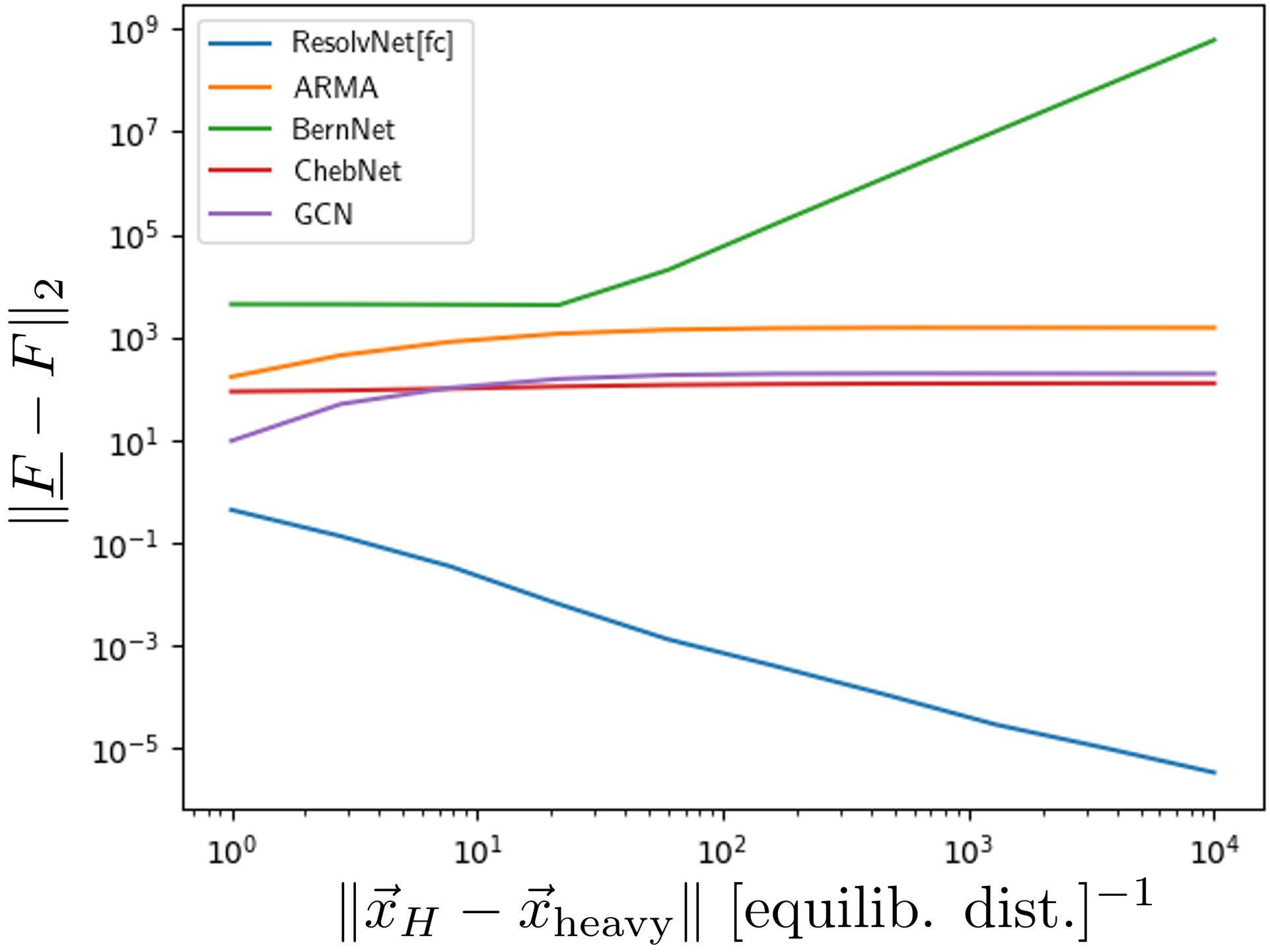
As a final experiment, we treat the coarse-grained molecular graphs as a model for data obtained from a resolution-limited observation process, that is unable to resolve positions of hydrogen and only provides information about how many H-atoms are bound to a given heavy atom. Given models trained on higher resolution data, atomization energies for such observed molecules are now to be predicted. Table 3 contains corresponding results. While the performance of baselines decreases significantly if the resolution scale is varied during inference, the prediction accuracy of ResolvNet remains high; even slightly increasing. While ResolvNet out-performed baselines by a factor of three on same-resolution-scale data (c.f.Table 2), its lead increases to a factor of and higher in the multi-scale setting. Table 3: QM-MAE QM MAE BernNet GCN ChebNet ARMA ResolvNet
6 Conclusion
This work introduced the concept of multi-scale consistency: At the node level this refers to the retention of a propagation scheme not solely determined by the largest given connectivity scale. At the graph-level it mandates that distinct graphs describing the same object at different resolutions should be assigned similar feature vectors. Common GNN architectures were shown to not be multi-scale consistent, while the newly introduced ResolvNet architecture was theoretically and experimentally established to have this property. Deployed on real world data, ResolvNet proved expressive and stable; out-performing baselines significantly on many tasks in- and outside the multi-scale setting.
References
- Alon & Yahav (2021) Uri Alon and Eran Yahav. On the bottleneck of graph neural networks and its practical implications. In International Conference on Learning Representations, 2021. URL https://openreview.net/forum?id=i80OPhOCVH2.
- Bárány & Solymosi (2017) Imre Bárány and József Solymosi. Gershgorin Disks for Multiple Eigenvalues of Non-negative Matrices, pp. 123–133. Springer International Publishing, Cham, 2017. doi: 10.1007/978-3-319-44479-6_6. URL https://doi.org/10.1007/978-3-319-44479-6_6.
- Bianchi et al. (2019) Filippo Maria Bianchi, Daniele Grattarola, Lorenzo Francesco Livi, and Cesare Alippi. Graph neural networks with convolutional arma filters. IEEE Transactions on Pattern Analysis and Machine Intelligence, 44:3496–3507, 2019.
- Blum & Reymond (2009) L. C. Blum and J.-L. Reymond. 970 million druglike small molecules for virtual screening in the chemical universe database GDB-13. J. Am. Chem. Soc., 131:8732, 2009.
- Bodnar et al. (2022) Cristian Bodnar, Francesco Di Giovanni, Benjamin Paul Chamberlain, Pietro Liò, and Michael M. Bronstein. Neural sheaf diffusion: A topological perspective on heterophily and oversmoothing in gnns. CoRR, abs/2202.04579, 2022. URL https://arxiv.org/abs/2202.04579.
- Brouwer & Haemers (2012) Andries E. Brouwer and Willem H. Haemers. Spectra of Graphs. New York, NY, 2012. doi: 10.1007/978-1-4614-1939-6.
- Chung (1997) F. R. K. Chung. Spectral Graph Theory. American Mathematical Society, 1997.
- Defferrard et al. (2016) Michaël Defferrard, Xavier Bresson, and Pierre Vandergheynst. Convolutional neural networks on graphs with fast localized spectral filtering. Advances in neural information processing systems, 29, 2016.
- Fey & Lenssen (2019) Matthias Fey and Jan E. Lenssen. Fast graph representation learning with PyTorch Geometric. In ICLR Workshop on Representation Learning on Graphs and Manifolds, 2019.
- Gao et al. (2023) Chen Gao, Yu Zheng, Nian Li, Yinfeng Li, Yingrong Qin, Jinghua Piao, Yuhan Quan, Jianxin Chang, Depeng Jin, Xiangnan He, and Yong Li. A survey of graph neural networks for recommender systems: Challenges, methods, and directions, 2023.
- Gasteiger et al. (2019a) Johannes Gasteiger, Aleksandar Bojchevski, and Stephan Günnemann. Predict then propagate: Graph neural networks meet personalized pagerank. In 7th International Conference on Learning Representations, ICLR 2019, New Orleans, LA, USA, May 6-9, 2019. OpenReview.net, 2019a. URL https://openreview.net/forum?id=H1gL-2A9Ym.
- Gasteiger et al. (2019b) Johannes Gasteiger, Aleksandar Bojchevski, and Stephan Günnemann. Predict then propagate: Graph neural networks meet personalized pagerank. In 7th International Conference on Learning Representations, ICLR 2019, New Orleans, LA, USA, May 6-9, 2019. OpenReview.net, 2019b. URL https://openreview.net/forum?id=H1gL-2A9Ym.
- Gilmer et al. (2017) Justin Gilmer, Samuel S Schoenholz, Patrick F Riley, Oriol Vinyals, and George E Dahl. Neural message passing for quantum chemistry. In International conference on machine learning, pp. 1263–1272. PMLR, 2017.
- Hamilton et al. (2017) William L. Hamilton, Zhitao Ying, and Jure Leskovec. Inductive representation learning on large graphs. In Isabelle Guyon, Ulrike von Luxburg, Samy Bengio, Hanna M. Wallach, Rob Fergus, S. V. N. Vishwanathan, and Roman Garnett (eds.), Advances in Neural Information Processing Systems 30: Annual Conference on Neural Information Processing Systems 2017, December 4-9, 2017, Long Beach, CA, USA, pp. 1024–1034, 2017. URL https://proceedings.neurips.cc/paper/2017/hash/5dd9db5e033da9c6fb5ba83c7a7ebea9-Abstract.html.
- He et al. (2021) Mingguo He, Zhewei Wei, Zengfeng Huang, and Hongteng Xu. Bernnet: Learning arbitrary graph spectral filters via bernstein approximation. In Marc’Aurelio Ranzato, Alina Beygelzimer, Yann N. Dauphin, Percy Liang, and Jennifer Wortman Vaughan (eds.), Advances in Neural Information Processing Systems 34: Annual Conference on Neural Information Processing Systems 2021, NeurIPS 2021, December 6-14, 2021, virtual, pp. 14239–14251, 2021. URL https://proceedings.neurips.cc/paper/2021/hash/76f1cfd7754a6e4fc3281bcccb3d0902-Abstract.html.
- Horn & Johnson (2012) Roger A Horn and Charles R Johnson. Matrix analysis. Cambridge university press, 2012.
- Hu et al. (2020) Weihua Hu, Matthias Fey, Marinka Zitnik, Yuxiao Dong, Hongyu Ren, Bowen Liu, Michele Catasta, and Jure Leskovec. Open graph benchmark: Datasets for machine learning on graphs. In Hugo Larochelle, Marc’Aurelio Ranzato, Raia Hadsell, Maria-Florina Balcan, and Hsuan-Tien Lin (eds.), Advances in Neural Information Processing Systems 33: Annual Conference on Neural Information Processing Systems 2020, NeurIPS 2020, December 6-12, 2020, virtual, 2020. URL https://proceedings.neurips.cc/paper/2020/hash/fb60d411a5c5b72b2e7d3527cfc84fd0-Abstract.html.
- Kato (1976) Tosio Kato. Perturbation theory for linear operators; 2nd ed. Grundlehren der mathematischen Wissenschaften : a series of comprehensive studies in mathematics. Springer, Berlin, 1976. URL https://cds.cern.ch/record/101545.
- Kipf & Welling (2017) Thomas N. Kipf and Max Welling. Semi-supervised classification with graph convolutional networks. In 5th International Conference on Learning Representations, ICLR 2017, Toulon, France, April 24-26, 2017, Conference Track Proceedings. OpenReview.net, 2017. URL https://openreview.net/forum?id=SJU4ayYgl.
- Koke (2023) Christian Koke. Limitless stability for graph convolutional networks. In 11th International Conference on Learning Representations, ICLR 2023, Kigali, Rwanda, May 1-5, 2023. OpenReview.net, 2023. URL https://openreview.net/forum?id=XqcQhVUr2h0.
- Levie et al. (2019) Ron Levie, Michael M. Bronstein, and Gitta Kutyniok. Transferability of spectral graph convolutional neural networks. CoRR, abs/1907.12972, 2019. URL http://arxiv.org/abs/1907.12972.
- Li et al. (2018a) Qimai Li, Zhichao Han, and Xiao-Ming Wu. Deeper insights into graph convolutional networks for semi-supervised learning. In Sheila A. McIlraith and Kilian Q. Weinberger (eds.), Proceedings of the Thirty-Second AAAI Conference on Artificial Intelligence, (AAAI-18), the 30th innovative Applications of Artificial Intelligence (IAAI-18), and the 8th AAAI Symposium on Educational Advances in Artificial Intelligence (EAAI-18), New Orleans, Louisiana, USA, February 2-7, 2018, pp. 3538–3545. AAAI Press, 2018a. doi: 10.1609/aaai.v32i1.11604. URL https://doi.org/10.1609/aaai.v32i1.11604.
- Li et al. (2018b) Yaguang Li, Rose Yu, Cyrus Shahabi, and Yan Liu. Diffusion convolutional recurrent neural network: Data-driven traffic forecasting. In 6th International Conference on Learning Representations, ICLR 2018, Vancouver, BC, Canada, April 30 - May 3, 2018, Conference Track Proceedings. OpenReview.net, 2018b. URL https://openreview.net/forum?id=SJiHXGWAZ.
- Maskey et al. (2021) Sohir Maskey, Ron Levie, and Gitta Kutyniok. Transferability of graph neural networks: an extended graphon approach. CoRR, abs/2109.10096, 2021. URL https://arxiv.org/abs/2109.10096.
- McCallum et al. (2000) Andrew McCallum, Kamal Nigam, Jason Rennie, and Kristie Seymore. Automating the construction of internet portals with machine learning. Inf. Retr., 3(2):127–163, 2000. doi: 10.1023/A:1009953814988. URL https://doi.org/10.1023/A:1009953814988.
- Namata et al. (2012) Galileo Namata, Ben London, Lise Getoor, and Bert Huang. Query-driven active surveying for collective classification. 2012.
- Oono & Suzuki (2020) Kenta Oono and Taiji Suzuki. Graph neural networks exponentially lose expressive power for node classification. In 8th International Conference on Learning Representations, ICLR 2020, Addis Ababa, Ethiopia, April 26-30, 2020. OpenReview.net, 2020. URL https://openreview.net/forum?id=S1ldO2EFPr.
- Pablo Gainza (2023) et. al. Pablo Gainza. Deciphering interaction fingerprints from protein molecular surfaces using geometric deep learning. Nature, 2023.
- Pei et al. (2020) Hongbin Pei, Bingzhe Wei, Kevin Chen-Chuan Chang, Yu Lei, and Bo Yang. Geom-gcn: Geometric graph convolutional networks, 2020. URL https://arxiv.org/abs/2002.05287.
- Post (2012) Olaf. Post. Spectral Analysis on Graph-like Spaces / by Olaf Post. Lecture Notes in Mathematics, 2039. Springer Berlin Heidelberg, Berlin, Heidelberg, 1st ed. 2012. edition, 2012. ISBN 3-642-23840-8.
- Post & Simmer (2021) Olaf Post and Jan Simmer. Graph-like spaces approximated by discrete graphs and applications. Mathematische Nachrichten, 294(11):2237–2278, 2021. doi: https://doi.org/10.1002/mana.201900108.
- Ramakrishnan et al. (2014) Raghunathan Ramakrishnan, Pavlo O Dral, Matthias Rupp, and O Anatole von Lilienfeld. Quantum chemistry structures and properties of 134 kilo molecules. Scientific Data, 1, 2014.
- Rozemberczki et al. (2021) Benedek Rozemberczki, Carl Allen, and Rik Sarkar. Multi-scale attributed node embedding. J. Complex Networks, 9(2), 2021. doi: 10.1093/comnet/cnab014. URL https://doi.org/10.1093/comnet/cnab014.
- Ruiz et al. (2020) Luana Ruiz, Luiz F. O. Chamon, and Alejandro Ribeiro. Graphon neural networks and the transferability of graph neural networks. In Hugo Larochelle, Marc’Aurelio Ranzato, Raia Hadsell, Maria-Florina Balcan, and Hsuan-Tien Lin (eds.), Advances in Neural Information Processing Systems 33: Annual Conference on Neural Information Processing Systems 2020, NeurIPS 2020, December 6-12, 2020, virtual, 2020. URL https://proceedings.neurips.cc/paper/2020/hash/12bcd658ef0a540cabc36cdf2b1046fd-Abstract.html.
- Rupp et al. (2012) M. Rupp, A. Tkatchenko, K.-R. Müller, and O. A. von Lilienfeld. Fast and accurate modeling of molecular atomization energies with machine learning. Physical Review Letters, 108:058301, 2012.
- Sen et al. (2008) Prithviraj Sen, Galileo Namata, Mustafa Bilgic, Lise Getoor, Brian Galligher, and Tina Eliassi-Rad. Collective classification in network data. AI Magazine, 29(3):93, Sep. 2008. doi: 10.1609/aimag.v29i3.2157. URL https://ojs.aaai.org/index.php/aimagazine/article/view/2157.
- Shchur et al. (2018) Oleksandr Shchur, Maximilian Mumme, Aleksandar Bojchevski, and Stephan Günnemann. Pitfalls of graph neural network evaluation. CoRR, abs/1811.05868, 2018. URL http://arxiv.org/abs/1811.05868.
- Shlomi et al. (2021) Jonathan Shlomi, Peter Battaglia, and Jean-Roch Vlimant. Graph neural networks in particle physics. Machine Learning: Science and Technology, 2(2):021001, jan 2021. doi: 10.1088/2632-2153/abbf9a. URL https://doi.org/10.1088%2F2632-2153%2Fabbf9a.
- Tang et al. (2009) Jie Tang, Jimeng Sun, Chi Wang, and Zi Yang. Social influence analysis in large-scale networks. In John F. Elder IV, Françoise Fogelman-Soulié, Peter A. Flach, and Mohammed Javeed Zaki (eds.), Proceedings of the 15th ACM SIGKDD International Conference on Knowledge Discovery and Data Mining, Paris, France, June 28 - July 1, 2009, pp. 807–816. ACM, 2009. doi: 10.1145/1557019.1557108. URL https://doi.org/10.1145/1557019.1557108.
- Teschl (2014) Gerald Teschl. Mathematical Methods in Quantum Mechanics. American Mathematical Society, 2014.
- Topping et al. (2021) Jake Topping, Francesco Di Giovanni, Benjamin Paul Chamberlain, Xiaowen Dong, and Michael M. Bronstein. Understanding over-squashing and bottlenecks on graphs via curvature, 2021. URL https://arxiv.org/abs/2111.14522.
- Velickovic et al. (2018) Petar Velickovic, Guillem Cucurull, Arantxa Casanova, Adriana Romero, Pietro Liò, and Yoshua Bengio. Graph attention networks. In 6th International Conference on Learning Representations, ICLR 2018, Vancouver, BC, Canada, April 30 - May 3, 2018, Conference Track Proceedings. OpenReview.net, 2018. URL https://openreview.net/forum?id=rJXMpikCZ.
- Wu et al. (2021) Zonghan Wu, Shirui Pan, Fengwen Chen, Guodong Long, Chengqi Zhang, and Philip S. Yu. A comprehensive survey on graph neural networks. IEEE Transactions on Neural Networks and Learning Systems, 32(1):4–24, jan 2021. doi: 10.1109/tnnls.2020.2978386. URL https://doi.org/10.1109%2Ftnnls.2020.2978386.
- Xiao et al. (2022) Shunxin Xiao, Shiping Wang, Yuanfei Dai, and Wenzhong Guo. Graph neural networks in node classification: survey and evaluation. Mach. Vis. Appl., 33(1):4, 2022. doi: 10.1007/s00138-021-01251-0. URL https://doi.org/10.1007/s00138-021-01251-0.
- Xu et al. (2019) Keyulu Xu, Weihua Hu, Jure Leskovec, and Stefanie Jegelka. How powerful are graph neural networks? In 7th International Conference on Learning Representations, ICLR 2019, New Orleans, LA, USA, May 6-9, 2019. OpenReview.net, 2019. URL https://openreview.net/forum?id=ryGs6iA5Km.
- Zhang et al. (2022) Linfeng Zhang, Han Wang, Maria Carolina Muniz, Athanassios Z. Panagiotopoulos, Roberto Car, and Weinan E. A deep potential model with long-range electrostatic interactions. The Journal of Chemical Physics, 156(12), mar 2022. doi: 10.1063/5.0083669. URL https://doi.org/10.1063%2F5.0083669.
- Zhang et al. (2021) Xitong Zhang, Yixuan He, Nathan Brugnone, Michael Perlmutter, and Matthew J. Hirn. Magnet: A neural network for directed graphs. In Marc’Aurelio Ranzato, Alina Beygelzimer, Yann N. Dauphin, Percy Liang, and Jennifer Wortman Vaughan (eds.), Advances in Neural Information Processing Systems 34: Annual Conference on Neural Information Processing Systems 2021, NeurIPS 2021, December 6-14, 2021, virtual, pp. 27003–27015, 2021. URL https://proceedings.neurips.cc/paper/2021/hash/e32084632d369461572832e6582aac36-Abstract.html.
Appendix A Effective Propagation Schemes
For definiteness, we here discuss limit-propagation schemes in the setting where edge-weights are large. The discussion for high-connectivity in the Sense of Example II of Section 2.1 proceeds in complete analogy.
In this section, we then take up again the setting of Section 2. We reformulate this setting here in a slightly modified language, that is more adapted to discussing effective propagation schemes of standard architectures:
We partition edges on a weighted graph , into two disjoint sets , where the set of edges with large weights is given by:
| (11) |
and the set with small weights is given by:
| (12) |
for weight scales . Without loss of generality, assume to be as low as possible (i.e. ) and to be as high as possible (i.e. ) and no weights in between the scales.
(a) (b) (c) (d)
This decomposition induces two graph structures corresponding to the disjoint edge sets on the node set : We set and c.f. Fig. 8).
We also introduce the set of edges
connecting nodes that do not have an incident edge in . A corresponding example-graph is depicted in Fig. 8 (d).
We are now interested in the behaviour of graph convolution schemes if the scales are well separated:
| (13) |
A.1 Spectral Convolutional Filters
We first discuss resulting limit-propagation schemes for spectral convolutional networks. Such networks implement convolutional filters as a mapping
| (14) |
for a node feature , a learnable function and a graph shift operator .
A.1.1 Need for Normalization
The graph shift operator facilitating the graph convolutions needs to be normalized for established spectral graph convolutional architectures:
For Bianchi et al. (2019), this e.g. arises as a necessity for convergence of the proposed implementation scheme for the rational filters introduced there (c.f. eq. (10) in Bianchi et al. (2019)).
The work Defferrard et al. (2016) needs its graph shift operator to be normalized, as it approximates generic filters via a Chebyshev expansion. As argued in Defferrard et al. (2016), such Chebyshev polynomials form an orthogonal basis for the space . Hence, the spectrum of the operator to which the (approximated and learned) function is applied needs to be contained in the interval .
In Kipf & Welling (2017), it has been noted that for the architecture proposed there, choosing to have eigenvalues in the range (as opposed to the normalized ranges or ) has the potential to lead to vanishing- or exploding gradients as well as numerical instabilities. To alleviate this, Kipf & Welling (2017) introduces a "renormalization trick" (c.f. Section 2.2. of Kipf & Welling (2017) to produce a normalized graph shift operator on which the network is then based.
We can understand the relationship between normalization of graph shift operator and the stability of corresponding convolutional filters explicitly: Assume that we have
| (15) |
This might e.g. happen when basing networks on the un-normalized graph Laplacian or the weight-matrix if edge weights are potentially large (such as in the setting that we are considering).
By the spectral mapping theorem (see e.g. Teschl (2014)), we have
| (16) |
with denoting the spectrum (i.e. the set of eigenvalues) of . For the largest (in absolute value) eigenvalue of , we have
| (17) |
Since learned functions are either implemented directly as a polynomial (as e.g. in Defferrard et al. (2016); He et al. (2021)) or approximated as a Neumann type power iteration (as e.g. in Bianchi et al. (2019); Gasteiger et al. (2019a)) which can be thought of as a polynomial, we have
| (18) |
Thus in view of (16) and (17) we have for sufficiently large, that
| (19) |
with the sign determined by . Since non-constant polynomials behave at least linearly for large inputs, there is a constant such that
| (20) |
for all sufficiently large . We thus have the estimate
| (21) |
for at least one input signal (more precisely all in the eigen-space corresponding to the largest (in absolute value) eigenvalue ). Thus if is not normalized (i.e. is not sufficiently bounded), the norm of (hidden) features might increase drastically when moving from one (hidden) layer to the next. This behaviour persists for all input signals have components in eigenspaces corresponding to large (in absolute value) eigenvalues of .
A.1.2 Spectral Normalizations
As discussed in the previous Section A.1.1, instabilities arising from non-normalized graph shift operators can be traced back to the problem of such operators having large eigenvalues. It was thus – among other considerations – suggested in Defferrard et al. (2016) to base convolutional filters on the spectrally normalized graph shift operator
| (22) |
with the un-normalized graph Laplacian. In the setting we are considering, this leads to an effective feature propagation along (c.f. also Fig. 9) only, as Theorem A.1 below establishes:
Theorem A.1.
Proof.
For convenience in notation, let us write
| (25) |
and similarly
| (26) |
In section 2, we already noted that
| (27) |
which we may rewrite as
| (28) |
Let us consider the equivalent expression
| (29) |
We next note that
| (30) |
and
| (31) |
since the operation of taking eigenvalues of operators is multiplicative in the sense of
| (32) |
for non-negative .
Since the right-hand-side of (29) constitutes an analytic perturbation of , we may apply analytic perturbation theory (c.f. e.g. Kato (1976) for an extensive discussion) to this problem. With this (together with ) we find
| (33) |
Using (30) and the fact that
| (34) |
we thus have
| (35) |
Since for small , we also have
| (36) |
the relation (34) also implies
| (37) |
Multiplying (28) with yields
| (38) |
Since and
| (39) |
for sufficiently large , relation (38) implies
| (40) |
as desired.
Note that we might in principle also make use of Lemma A.2 below, to provide quantitative bounds: Lemma A.2 states that
| (41) |
for self-adjoint operators and and their respective eigenvalues ordered by magnitude. On a graph with nodes, we clearly have for eigenvalues of (rescaled) graph Laplacians, since all such eigenvalues are non-negative. This implies for the difference arising in (33) that explicitly
| (42) |
This in turn can then be used to provide a quantitative bound in (24). Since we are only interested in the qualitative behaviour for , we shall however not pursue this further.
∎
Lemma A.2.
Let and be two hermitian dimensional matrices. Denote by
the eigenvalues of a hermitian matrix in increasing order.
With this we have:
| (43) |
Proof.
After the redefinition , what we need to prove is
| (44) |
for Hermitian . Since we have
| (45) |
and it follows that it suffices to prove
| (46) |
for arbitrary hermitian .
We note that the Courant-Fischer theorem tells us that if is an Hermitian matrix, we have
| (47) |
With this we find
| (48) | ||||
| (49) | ||||
| (50) | ||||
| (51) | ||||
| (52) | ||||
| (53) | ||||
| (54) |
∎
A.1.3 Symmetric Normalizations
Most common spectral graph convolutional networks (such as e.g. He et al. (2021); Bianchi et al. (2019); Defferrard et al. (2016)) base the learnable filters that they propose on the symmetrically normalized graph Laplacian
| (55) |
In the setting we are considering, this leads to an effective feature propagation along edges in and (c.f. also Fig. 10) only, as Theorem A.3 below establishes:
Theorem A.3.
Proof.
We first note that instead of (57), we may equivalently establish
| (58) |
In Section 2, we already noted that
| (59) |
With this, we may write
| (60) |
Let us first examine the term . We note for the corresponding matrix entries that
| (61) |
Let us use the notation
| (62) |
We then find
| (63) |
Using the Taylor expansion
| (64) |
we thus have
| (65) |
Since we have
| (66) |
this yields
| (67) |
Thus let us turn towards the second summand on the right-hand-side of (60). We have
| (68) |
Suppose that either or is not in . Without loss of generality (since the matrix under consideration is symmetric), assume , but . We may again write
| (69) |
Since
| (70) |
we have
| (71) |
If instead we have , then clearly
| (72) |
Thus in total we have established
| (73) |
which was to be established.
∎
Apart from networks that make use of the symmetrically normalized graph Laplacian , some methods, such as most notably Kipf & Welling (2017), instead base their filters on the operator
| (74) |
with
| (75) |
and
| (76) |
In analogy to Theorem A.3, we here establish the limit propagation scheme determined by such operators:
Theorem A.4.
With
| (77) |
where and as well as the scale decompositionof Section 2, we have that
| (78) |
for . Here is given as
| (79) |
and denotes the vector whose entries are one for nodes in and zero for all other nodes.
The difference to the result of Theorem A.3 is thus that applicability of the limit propagation scheme of Fig. 10 for the GCN Kipf & Welling (2017) is not only contingent upon but also .
Proof.
To establish this – as in the proof of Theorem A.3 – we first decompose :
| (80) | ||||
| (81) |
For the first term, we note
| (82) |
We then find
| (83) |
Analogously to the proof of Theorem A.3, this yields
| (84) |
This implies
| (85) |
Next we turn to the second summand in (80):
| (86) |
Suppose that either or is not in . Without loss of generality (since the matrix under consideration is symmetric), assume , but . We may again write
| (87) |
Since
| (88) |
we have
| (89) | ||||
| (90) | ||||
| (91) |
If instead we have , then clearly
| (92) |
In total we thus have found
| (94) |
which was to be proved. ∎
A.2 Spatial Convolutional Filters
Apart from spectral methods, there of course also exist methods that purely operate in the spatial domain of the graph. Such methods most often fall into the paradigm of message passing neural networks (MPNNs) Gilmer et al. (2017); Fey & Lenssen (2019): With denoting the features of node in layer and denoting edge features, a message passing neural network may be described by the update rule (c.f. Gilmer et al. (2017))
| (95) |
Here denotes the neighbourhood of node , denotes a differentiable and permutation invariant function (typically "sum", "mean" or "max") while and denote differentiable functions such as multi-layer-perceptrons (MLPs) which might not be the same in each layer. Fey & Lenssen (2019).
Before we discuss corresponding limit-propagation schemes, we first establish that MPNNs are not able to reproduce the limit propagation scheme of Section 3 and are thus not stable to scale transitions and topological perturbations as discussed in Theorem 4.2 and Section 2.2.2.
A.2.1 Scale-Sensitivity of Message Passing Neural Networks
As we established in Theorem 4.1 and Theorem 4.2 (c.f. also the corresponding proofs in Appendix D and Appendix E respectively), the stability to scale-variations (such as coarse-graining) of ResolvNets arises from the reliance on resolvents and the limit propagation scheme that they establish if separated weight-scales are present (c.f. Appendix B below).
Here we establish that message passing networks (as defined in (95) above) are unable to emulate this limit propagation scheme. Hence such architectures are also not stable to scale-changing topological perturbations such as coarse-graining procedures.
To this end, we consider a simple, fully connected graph on three nodes labeled , and (c.f. Fig. 11). We assume all node-weights to be equal to one ( for ) and edge weights
| (96) |
as well as
| (97) |
We now assume .
Given states in layer , the limit propagation scheme introduced in Section 3 would require the updated feature vector of node to be given by
| (98) |
However, the actual updated feature at node is given as (c.f. (95)):
| (99) |
Since there is no dependence on in equation (99) – which defines – the desired propagation scheme can not arise, unless it is paradoxically already present at all scales . If it is present at all scales, there is however only propagation along edges in , even if , which would imply that the message passing network would not respect the graph structure of . Hence does not converge as increases.
A.2.2 Limit Propagation Schemes
The number of possible choices of message functions , aggregation functions and update functions is clearly endless. Here we shall exemplarily discuss limit propagation schemes for two popular architectures: We first discuss the most general case where the message function is given as a learnable perceptron. Subsequently we assume that node features are updated with an attention-type mechanism.
Generic message functions:
We first consider the possibility that the message function in (99) is implemented via an MLP using ReLU-activations: Assuming (for simplicity in notation) a one-hidden-layer MLP mapping features to features we have
| (100) |
with bias term and weight matrices and .
We will assume that the weight-vecor has no-nonzero entries. This is not a severe limitation experimentally and in fact generically justified: The complementary event of at-least one entry of being assigned precisely zero during training has probability weight zero (assuming an absolutely continuous probability distribtuion according to which weights are learned).
Let us now assume that the edge belongs to and the corresponding weight is large (). The behaviour of entries of the message is then determined by the sign of the corresponding entry of the weight vector :
If we have , then approaches zero for larger edge-weights :
| (101) |
If we have , then increasingly diverges for larger edge-weights :
| (102) |
For either choice of aggregation function in (95) among "max", "sum" or "mean" the behaviour in (102) leads to unstable networks if the update function is also given as an MLP with ReLU activations. Apart from instabilities, we also make the following observation: If , then by (102) and continuity of we can conclude that components of messages propagated along for which dominate over messages propagated along edges in . By (101), the former clearly also dominate over components of messages propagated along for which . This behaviour is irrespective of whether "max", "sum" or "mean" aggregations are employed. Hence the limit propagation scheme essentially only takes into account message channels for which and .
Similar considerations apply, if non-linearities are chosen as leaky ReLU. If instead of ReLU activations a sigmoid-nonlinearity like is employed, messages propagated along become increasingly uninformative, since they are progressively more independent of features and weights . Indeed, for sigmoid activations, the limits (101) and (102) are given as follows:
If we have , then we have for larger edge-weights that
| (103) |
If we have , then
| (104) |
In both cases, the messages propagated along become increasingly constant as the scale increases.
Attention based messages:
Apart from general learnable message functions as above, we here also discuss an approach where edge weights are re-learned in an attention based manner. For this we modify the method Velickovic et al. (2018) to include edge weights. The resulting propagation scheme – with a single attention head for simplicity and a non-linearity – is given as
| (105) |
Here we have and
| (106) |
with denoting concatenation. The weight vector is assumed to have a non zero entry in its last component. Otherwise, this attention mechanism would correspond to the one proposed in Velickovic et al. (2018), which does not take into account edge weights. Let us denote this entry of ()determining attention on the weight ) by .
If , we have for that
| (107) |
as the weight increases. Thus propagation along edges in is essentially suppressed in this case.
If , we have for that
| (108) |
as the weight increases. Thus for edges (i.e. those that are not in ), we have
| (109) |
since the denominator in (106) diverges. Hence in this case, propagation along is essentially suppressed and features are effectively only propagated along .
Appendix B Proof of Theorem 3.3
In this section, we prove Theorem 3.3. For convenience, we first restate the result – together with the definitions leading up to it – again:
Definition B.1.
Denote by the set of connected components in . We give this set a graph structure as follows: Let and be elements of (i.e. connected components in ). We define the real number
| (110) |
with and nodes in the original graph . We define the set of edges on as
| (111) |
and assign as weight to such edges. Node weights of limit nodes are defined similarly as aggregated weights of all nodes (in ) contained in the component as
| (112) |
In order to translate signals between the original graph and the limit description , we need translation operators mapping signals from one graph to the other:
Definition B.2.
Denote by the vector that has as entries on nodes belonging to the connected (in ) component and has entry zero for all nodes not in . We define the down-projection operator component-wise via evaluating at node in as
| (113) |
The upsampling operator is defined as
| (114) |
where is a scalar value (the component entry of at ) and the sum is taken over all connected components in .
The result we then have to prove is the following:
Theorem B.3.
We have
| (115) |
holds; with denoting the first non-zero eigenvalue of .
Note that this then indeed proves Theorem 3.3, since we have
| (116) |
Proof.
We will split the proof of this result into multiple steps. For Let us denote by
| (117) | ||||
| (118) | ||||
| (119) |
the resolvents correspodning to , and respectively.
Our first goal is establishing that we may write
| (120) |
This will follow as a consequence of what is called the second resolvent formula Teschl (2014):
"Given self-adjoint operators , we may write
| (121) |
In our case, this translates to
| (122) |
or equivalently
| (123) |
Multiplying with from the left then yields
| (124) |
as desired.
Hence we need to establish that is invertible for .
To establish a contradiction, assume it is not invertible. Then there is a signal such that
| (125) |
Multiplying with from the left yields
| (126) |
which is precisely to say that
| (127) |
But since is a graph Laplacian, it only has non-negative eigenvalues. Hence we have reached our contradiction and established
| (128) |
Our next step is to establish that
| (129) |
where is the spectral projection onto the eigenspace corresponding to the lowest lying eigenvalue of . Indeed, by the spectral theorem for finite dimensional operators (c.f. e.g. Teschl (2014)), we may write
| (130) |
Here denotes the spectrum (i.e. the collection of eigenvalues) of and the are the corresponding (orthogonal) eigenprojections onto the eigenspaces of the respective eigenvalues. Thus we find
| (131) |
where the sum on the right hand side now excludes the eigenvalue .
Using orthonormality of the spectral projections, the fact that and monotonicity of we find
| (132) |
Here is the firt non-zero eigenvalue of .
Non-zero eigenvalues scale linearly with the weight scale since we have
| (133) |
for any graph Laplacian (in fact any matrix) with eigenvalue . Thus we have
| (134) |
as .
Our next task is to use this result in order to bound the difference
| (135) |
To this end we first note that the relation
| (136) |
provided to us by the second resolvent formula, implies
| (137) |
Thus we have
| (138) | ||||
| (139) |
With this, we have
| (140) | ||||
| (141) | ||||
| (142) | ||||
| (143) |
Hence it remains to bound the left hand summand. For this we use the following fact (c.f. Horn & Johnson (2012), Section 5.8. "Condition numbers: inverses and linear systems"):
Given square matrices with and , we have
| (144) |
In our case, this yields (together with ) that
| (145) | ||||
| (146) |
For sufficiently large, we have
| (147) |
so that we may estimate
| (148) | ||||
| (149) | ||||
| (150) |
Thus we have now established
| (151) |
Hence we are done with the proof, as soon as we can establish
| (152) |
with as defined above. To this end, we first note that
| (153) |
and
| (154) |
Indeed,the relation (153) follows from the fact that the eigenspace corresponding to the eignvalue zero is spanned by the vectors , with the connected components of . Equation (154) follows from the fact that
| (155) |
With this we have
| (156) |
To proceed, set
| (157) |
and
| (158) |
Then
| (159) |
and hence . Thus we have
| (160) |
Multiplying with from the left yields
| (161) |
Thus we have
| (162) |
This – in turn – implies
| (163) |
Using
| (164) |
we then have
| (165) |
We have thus concluded the proof if we can prove that is the Laplacian corresponding to the graph defined in Definition B.1. But this is a straightforward calculation. ∎
As a corollary, we find
Corollary B.4.
We have
| (166) |
Proof.
This follows directly from the fact that
| (167) |
∎
Appendix C Proof of Theorem 3.4
Here we prove Theorem 3.4, which we restate for convenience:
Theorem C.1.
Fix and . For arbitrary functions with and , there are filters of Type- and Type-I respectively such that .
Proof.
The Stone-Weierstrass theorem (see e.g. Teschl (2014)) states that any sub-algebra of continuous functions that are constant at infinity is already dense (in the topoloogy of uniform convergence) if this sub-algebra separates points.
Thus – using the Stone-Weierstrass Theorem – all we have to prove to establish the claim is that for every pair of points there is a function with
| (168) |
But this is clear since (for ) the function
| (169) |
(which generates the algebra of functions we consider) is already everywhere defined and injective. ∎
Appendix D Stability Theory
Here we provide stability results to input- and edge-weight- perturbations for our architecture. For convenience, we restate our layer-wise update rule here again:
Given a feature matrix in layer , with column vectors , the feature vector in layer is calculated as with a learnable bias vector . Collecting biases into a matrix , we efficiently implement this using matrix-multiplications as
| (170) |
with weight matrices in . Biases are implemented as , with the vector of all ones on and learnable.
Our first result main-body of the paper then concerns stability to perturbations of input signals:
Theorem D.1.
Let be the map associated to an -layer deep ResolvNet. Denote the collection of weight matrices in layer by . We have
| (171) |
with
| (172) |
aggregating singular values of weight matrices.
Proof.
Let us denote (hidden) feature matrices in layer by (resp. ).
We note the following:
| (173) | ||||
| (174) | ||||
| (175) | ||||
| (176) | ||||
| (177) | ||||
| (178) |
Iterating through the layers yields the desired inequality (171). ∎
In preparation for our next result – Theorem D.5 below – we note the following:
Lemma D.2.
Let be the map associated to an -layer deep ResolvNet. With weights and biases denoted as above, we have
| (179) |
Proof.
Before we can establish Theorem D.5 below, we need two additional (related) preliminary results:
Lemma D.3.
Let us use the notation and for resulvents corresponding to two different Laplacians and . We have
| (185) |
Proof.
Let and be (finite dimensional) operators. Choose so that it is neither an eigenvalue of nor .
To showcase the principles underlying the proof, let us use the notation
| (186) |
We note the following
| (187) | ||||
| (188) | ||||
| (189) | ||||
| (190) |
Rearranging and using
| (191) |
together with the sub-multiplicativity of the operator-norm yields the claim. ∎
We also note the following estimate on differences of powers of resolvents:
Lemma D.4.
Let and . For any natural number , we have
| (192) |
Proof.
We note that for arbitrary matrices , we have
| (193) | ||||
| (194) |
Iterating this and using
| (195) |
for then yields the claim. ∎
Having established the preceding lemmata, we can now establish stability to perturbations of the edge weights:
Theorem D.5.
Let and be the maps associated to ResolvNets with the same network architecture, but based on Laplacians and respectively. We have
| (196) |
Here, the stability constants and are polynomials in (the largest) singular values of weight matrices and weight matrices as well as bias matrices, respectively.
Proof.
Denote by and the (hidden) feature matrices generated in layer for networks based on Laplacians and respectively: I.e. we have
| (197) |
and
| (198) |
Using the fact that is Lipschitz continuous with Lipschitz constant , we have
| (199) | ||||
| (200) | ||||
| (201) | ||||
| (202) | ||||
| (203) | ||||
| (204) | ||||
| (205) |
Applying Lemma D.4 yields
| (207) | ||||
| (208) |
Using Lemma D.3, we then have
| (210) | ||||
| (211) |
Appendix E Stability under Scale Variations
Here we provide details on the scale-invariance results discussed in Section 4.
In preparation, we will first need to prove a lemma relating powers of resolvents on the original graph and its limit-description :
Lemma E.1.
Let and . For any natural number , we have
| (217) |
The proof proceeds in analogy to that of Lemma D.4:
Proof.
We note that for arbitrary matrices , we have
| (218) | ||||
| (219) |
Iterating this, using
| (220) |
for together with and
| (221) |
(which holds since ) then yields the claim.
Note that the equation
| (222) |
holds, because we may write
| (223) |
∎
Hence let us now prove Stability-Theorem 4.1, which we restate here for convenience:
Theorem E.2.
Let and be the maps associated to ResolvNets with the same learned weight matrices and biases but deployed on graphs and as defined in Section 2.2.2 . We have
| (224) |
if the network is based on Type- resolvent filters (c.f. Section 3). Additionally, we have
| (225) |
if only Type-I filters are used in the network. Here and are constants that depend polynomially on singular values of learned weight matrices and biases .
Proof.
Denote by and the (hidden) feature matrices generated in layer for networks based on resolvents and respectively: I.e. we have
| (227) |
and
| (228) |
Here, since bias terms are proportional to constant vectors on the graphs, as detailed in Section 3, we have
| (229) |
and
| (230) |
for bias matrices and in networks deployed on and respectively.
We then have
| (231) | ||||
| (232) | ||||
| (233) | ||||
| (234) |
Here we used the fact that since maps positive entries to positive entries and acts pointwise, it commutes with . We also made use of (230).
Using the fact that is Lipschitz-continuous with Lipschitz constant , we can establish
| (235) |
Using the fact that , we have
| (236) |
From this, we find (using ), that
| (237) | ||||
| (238) | ||||
| (239) | ||||
| (240) | ||||
| (241) |
Applying Lemma E.1 yields
| (243) | ||||
| (244) |
Lemma then D.2 in Appendix D established that we have
| (246) |
Hence the summand on the left-hand-side can be bounded in terms of a polynomial in singular values of bias- and weight matrices, as well as and most importantly the factor which tends to zero.
For the summand on the right-hand-side, we can iterate the above procedure (aggregating terms like (246) multiplied by ) until reaching the last layer . There we observe
| (247) | ||||
| (248) | ||||
| (249) | ||||
| (250) | ||||
| (251) |
The last step is only possible because we let the sums over powers of resolvents start at as opposed to . In the latter case, there would have remained a term , which would not decay as .
Aggregating terms, we build up the polynomial stability constants of (225) layer by layer, and complete the proof.
The proof of (224) proceeds in complete analogy upon defining
| (252) |
Note that starting with on , implies that we have
| (253) |
This avoids any complications arising from employing Type- filters in this setting.
∎
Next we transfer the previous result to the graph level setting:
Theorem E.3.
Proof.
Let us first recall that our aggregation scheme mapped a feature matrix to a graph-level feature vector defined component-wise as
| (255) |
In light of Theorem E.2, we are done with the proof, once we have established that
| (256) |
To this end, we first note that
| (257) |
Indeed, this follows from the fact that given a connected component in , the map assigns the same feature vector to each node (c.f. (114)), together with the fact that
| (258) |
Thus we have
| (259) |
Next let us simplify notation and write
| (260) |
and
| (261) |
with . We note:
| (262) |
By means of the Cauchy-Schwarz inequality together with the inverse triangle-inequality, we have
| (263) | ||||
| (264) |
Since we have
| (265) |
the claim is established. ∎
Appendix F Additional Details on Experiments:
All experiments were performed on a single NVIDIA Quadro RTX 8000 graphics card.
F.1 Node Classification
Datasets:
We test our approach for the task of node-classification on eight different standard datasets across the entire homophily-spectrum. Among these, Citeseer Sen et al. (2008), Cora-ML McCallum et al. (2000) and PubMed Namata et al. (2012) are citation graphs. Here each node represents a paper and edges correspond to citations. We also test on the Microsoft Academic graph Shchur et al. (2018) where an edge that is present corresponds to co-authorship. Bag-of-word representations act as node features. The WebKB datasets Cornell and Texas are datasets modeling links between websites at computer science departments of various universitiesPei et al. (2020). Node features are bag-of-words representation of the respective web pages. We also consider the actor co-occurence dataset Actor Tang et al. (2009) as well as the Wikipedia based dataset Squirrel Rozemberczki et al. (2021).
Experimental setup
We closely follow the experimental setup of Gasteiger et al. (2019b) on which our codebase builds: All models are trained for a fixed maximum (and unreachably high) number of epochs. Early stopping is performed when the validation performance has not improved for epochs. Test-results for the parameter set achieving the highest validation-accuracy are then reported. Ties are broken by selecting the lowest loss (c.f. Velickovic et al. (2018); Gasteiger et al. (2019a)). Confidence intervals are calculated over multiple splits and random seeds at the confidence level via bootstrapping.
Additional details on training and models:
We train all models on a fixed learning rate of
| (266) |
Global dropout probability of all models is optimized individually over
| (267) |
We use weight decay and optimize the weight decay parameter for all models over
| (268) |
Where applicable (i.e. not for Gasteiger et al. (2019a); He et al. (2021)) we choose a two-layer deep convolutional architecture with the dimensions of hidden features optimized over
| (269) |
In addition to the hyperparemeters specified above, some baselines have additional hyperparameters, which we detail here: BernNet uses an additional in-layer dropout rate of and for its filters a polynomial order of as suggested in He et al. (2021). As suggested in Gasteiger et al. (2019a), the hyperparameter of PPNP is set to on the MS_Academic dataset and to on other datasets. Hyperparameters depth and number of stacks of the ARMA convolutional layer Bianchi et al. (2019) are set to and . ChebNet also uses to avoid the known over-fitting issue Kipf & Welling (2017) for higher polynomial orders. For MagNet we use as suggested in Zhang et al. (2021) and choose the parameter as given in Table 1 of Zhang et al. (2021) for the respective datasets. The graph attention network Velickovic et al. (2018) uses attention heads, as suggested in Velickovic et al. (2018).
For our ResolvNet model, we choose a depth of with hidden feature dimension optimized over the values in (269) as for baselines. We empirically observed in the setting of unweighted graphs, that rescaling the Laplacian as
| (270) |
with a normalizing factor before calculating the resolvent
| (271) |
on which we base our ResolvNet architectures improved performance.
For our ResolvNet architecture, we express this normalizing factor in terms of the largest singular value of the (non-normalized) graph Laplacian. It is then selected among
| (272) |
The value in (271) is selected among
| (273) |
We base our ResolvNet architecture on Type-0 filters and choose the maximum resolvent-exponent as .
F.2 Graph Regression
Datasets:
The first dataset we consider is the QM dataset, introduced in Blum & Reymond (2009); Rupp et al. (2012). This dataset contains descriptions of organic molecules, each with up to seven heavy atoms, with all non-hydrogen atoms being considered heavy. A molecule is represented by its Coulomb matrix , whose off-diagonal elements
| (274) |
correspond to the Coulomb-repulsion between atoms and . We discard diagonal entries of Coulomb matrices; which would encode a polynomial fit of atomic energies to nuclear charge Rupp et al. (2012).
For each atom in any given molecular graph, the individual Cartesian coordinates and the atomic charge are also accessible individually. To each molecule an atomization energy - calculated via density functional theory - is associated. The objective is to predict this quantity. The performance metric is mean absolute error. Numerically, atomization energies are negative numbers in the range to . The associated unit is .
The second dataset we consider is the QM dataset Ramakrishnan et al. (2014), which consists of roughly 130 000 molecules in equilibrium. Beyond atomization energy, there are in total targets available on QM. We provide a complete list of targets together with abbreviations in Table 4 below:
| Symbol | Property | Unit |
|---|---|---|
| Internal energy at | ||
| Internal energy at | ||
| Enthalpy at | ||
| Free energy at | ||
| Atomization energy at | ||
| Atomization energy at | ||
| Atomization enthalpy at | ||
| Atomization free energy at | ||
| Heat capacity at | ||
| Dipole moment | ||
| Isotropic polarizability | ||
| Highest occupied molecular orbital energy | ||
| Lowest unoccupied molecular orbital energy | ||
| Gap between and | ||
| Electronic spatial extent | ||
| ZPVE | Zero point vibrational energy | |
| A | Rotational constant | |
| B | Rotational constant | |
| C | Rotational constant |
Molecules in QM are not directly encoded via their Coulomb-matrices, as in QM. However, positions and charges of individual molecules are available, from which the Coulomb matrix description is calculated for each molecule.
Experimental Setup:
On both datasets, we randomly select molecules for testing and train on the remaining graphs. On QM we run experiments for different random random seeds and report mean and standard deviation. Due to computational limitations we run experiments for different random seeds on the larger QM dataset, and report mean and standard deviation.
Additional details on training and models:
All considered convolutional layers are incorporated into a two layer deep and fully connected graph convolutional architecture. In each hidden layer, we set the width (i.e. the hidden feature dimension) to
| (275) |
For BernNet, we set the polynomial order to to combat appearing numerical instabilities. ARMA is set to and . ChebNet uses . For all baselines, the standard mean-aggregation scheme is employed after the graph-convolutional layers to generate graph level features. Finally, predictions are generated via an MLP.
For our model, we choose a two-layer deep instantiation of our ResolvNet architecture introduced in Section 3. We choose Type-I filters and set . Laplacians are not rescaled and resolvents are thus given as
| (276) |
As aggregation, we employ the graph level feature aggregation scheme introduced at the end of Section 3 with node weights set to atomic charges of individual atoms. Predictions are then generated via a final MLP with the same specifications as the one used for baselines.
All models are trained independently on each respective target.
Results:
Beyond the results already showcased in the main body of the paper, we here provide results for ResolvNet as well as baselines on all targets of Table 4. These results are collected in Table 5, Table 6 and Table 7 below.
As is evident from the tables, the ResolvNet architecture produces mean-absolute-errors comparable to those of baselines on of targets, while it performs significantly better on of targets.
The difference in performance is especially significant on the (extensive) energy targets of Table 5. In this Table, baselines are out-performed by factors varying between and .
Table 6 contains three additional targets where MAEs produced by ResolvNet are lower by factors varying between roughly two and four, when compared to baselines.
Table 7 finally contains MAEs corresponding to predictions of rotational constants. Here our model yields a comparable error on one target and provides better results than baselines on two out of three targets.
| Property | ||||||||
|---|---|---|---|---|---|---|---|---|
| BernNet | ||||||||
| GCN | ||||||||
| ChebNet | ||||||||
| ARMA | ||||||||
| R.N. |
| Property | ZPVE | |||||||
|---|---|---|---|---|---|---|---|---|
| BernNet | ||||||||
| GCN | ||||||||
| ChebNet | ||||||||
| ARMA | ||||||||
| R.N. |
| Property | |||
|---|---|---|---|
| BernNet | |||
| GCN | |||
| ChebNet | |||
| ARMA | |||
| R.N. |
F.3 Scale Invariance
Dataset:
Again, we make use of the QM dataset Rupp et al. (2012) and its Coulomb matrix description
| (277) |
of molecules.
Details on collapsing procedure:
We modify (all) molecular graphs in QM by deflecting hydrogen atoms (H) out of their equilibrium positions towards the respective nearest heavy atom. This is possible since the QM dataset also contains the Cartesian coordinates of individual atoms.
This introduces a two-scale setting precisely as discussed in section 2: Edge weights between heavy atoms remain the same, while Coulomb repulsions between H-atoms and respective nearest heavy atom increasingly diverge; as is evident from (277).
Given an original molecular graph with node weights , the corresponding limit graph corresponds to a coarse grained description, where heavy atoms and surrounding H-atoms are aggregated into single super-nodes in the sense of Section 2.2.2 .
Mathematically, is obtained by removing all nodes corresponding to H-atoms from , while adding the corresponding charges to the node-weights of the respective nearest heavy atom. Charges in (277) are modified similarly to generate the weight matrix .
On original molecular graphs, atomic charges are provided via one-hot encodings. For the graph of methane – consisting of one carbon atom with charge and four hydrogen atoms of charges – the corresponding node-feature-matrix is e.g. given as
| (278) |
with the non-zero entry in the first row being in the column, in order to encode the charge for carbon.
The feature vector of an aggregated node represents charges of the heavy atom and its neighbouring H-atoms jointly.
As discussed in Definition 3.2, node feature matrices are translated as . Applying to one-hot encoded atomic charges yields (normalized) bag-of-word embeddings on : Individual entries of feature vectors encode how much of the total charge of the super-node is contributed by individual atom-types. In the example of methane, the limit graph consists of a single node with node-weight
| (279) |
The feature matrix
| (280) |
is a single row-vector given as
| (281) |
Results:
For convenience, we repeat here in Table 8 and Figure 12 the results corresponding to the use of resolution-limited data in the form of coarse-grained molecular graphs during inference, that were already presented in the main body of the paper.
| QM | MAE |
|---|---|
| BernNet | |
| GCN | |
| ChebNet | |
| ARMA | |
| ResolvNet |
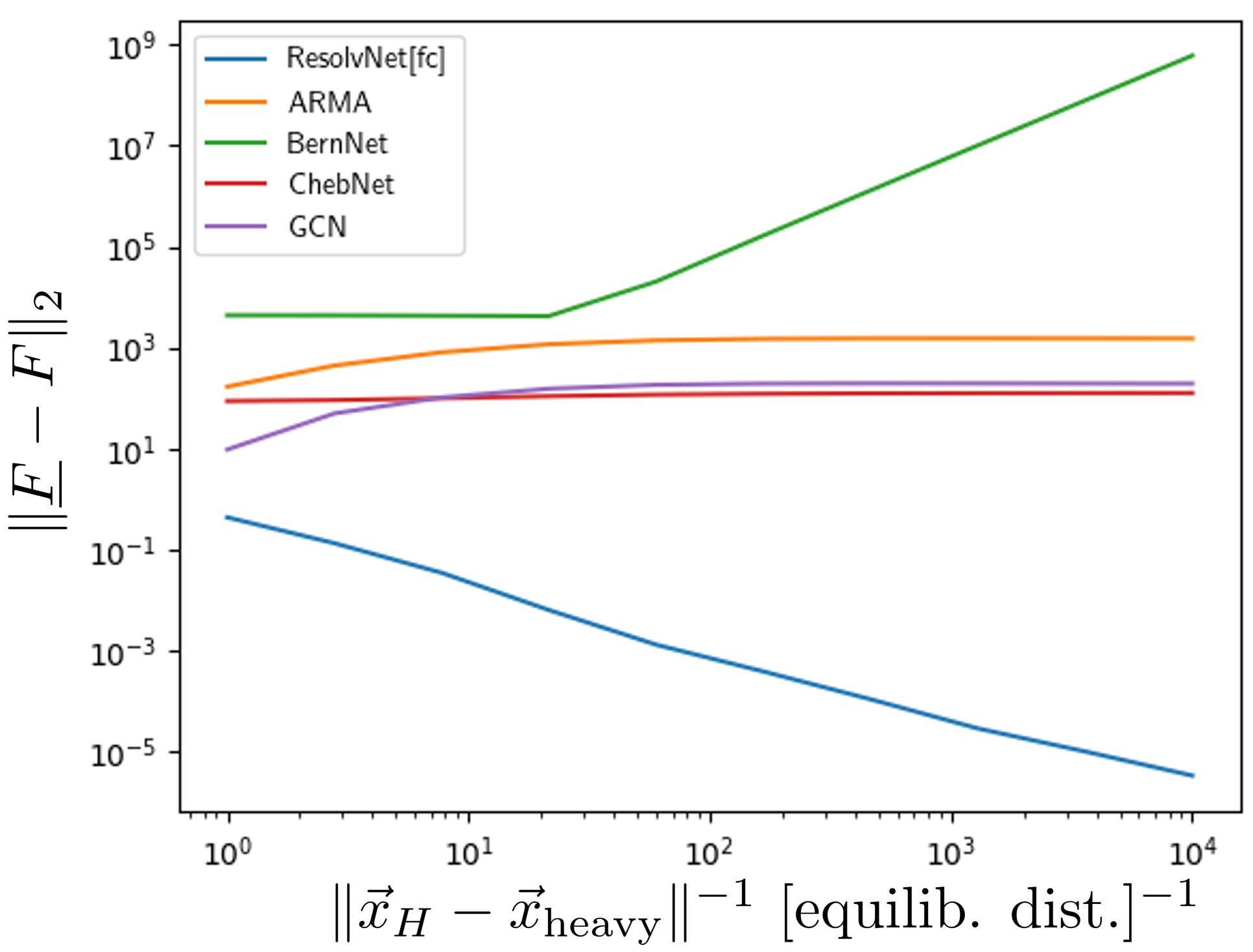
Appendix G Analysis of Computational Overhead
Here we provide an analysis of the overhead of our ResolvNet method. As is evident from Tables 9, 10, 11 below, on most datasets our method is not the most memory intensive to train when compared to representative (spatial and spectral) baselines. For training times (total and per-epoch), we note that on most small to medium sized graphs, our model is not the slowest to train. On larger graphs it does take longer to train. Regarding complexity, the node update for our model is essentially (dense-dense matrix multiplication), while message passing baselines scale linearly in the number of edges.
| MS_Acad. | Cora | Pubmed | Citeseer | Cornell | Actor | Squirrel | Texas | |
|---|---|---|---|---|---|---|---|---|
| ResolvNet | 3.47 | 0.1266 | 2.9915 | 0.0996 | 0.0070 | 0.4936 | 0.2915 | 0.0175 |
| GAT | 1.49 | 0.1559 | 0.6486 | 0.1105 | 0.0228 | 0.3666 | 2.1107 | 0.0219 |
| ChebNet | 10.19 | 0.4741 | 0.4848 | 0.3389 | 0.0249 | 0.4830 | 6.3569 | 0.0241 |
| MS_Acad. | Cora | Pubmed | Citeseer | Cornell | Actor | Squirrel | Texas | |
|---|---|---|---|---|---|---|---|---|
| ResolvNet | 474.409 | 3.671 | 34.140 | 1.387 | 1.745 | 9.623 | 4.874 | 0.875 |
| GAT | 34.388 | 2.194 | 5.741 | 0.891 | 2.123 | 1.610 | 23.060 | 1.375 |
| ChebNet | 87.567 | 6.818 | 3.221 | 2.833 | 2.713 | 1.488 | 14.383 | 4.511 |
| MS_Acad. | Cora | Pubmed | Citeseer | Cornell | Actor | Squirrel | Texas | |
|---|---|---|---|---|---|---|---|---|
| ResolvNet | 1359.34 | 13.16 | 161.80 | 11.01 | 2.58 | 32.51 | 41.30 | 2.54 |
| GAT | 60.01 | 8.22 | 29.59 | 7.24 | 3.93 | 15.05 | 62.49 | 4.07 |
| ChebNet | 202.23 | 12.11 | 14.31 | 10.61 | 3.89 | 13.28 | 126.17 | 3.83 |
