On Learning with LAD

Suppose we have a collection of observations for a particular phenomenon in the form of data points and the information about its occurrence at each data point. We refer to such a data set as the training set. Data points are (feature) vectors whose coordinates are values of variables called features. The information on the occurrence or non-occurrence of the phenomenon under consideration can be recorded by labeling each data point as a “false” point or a “true” point, alternatively, by $0$ or $1$, respectively. Peter L. Hammer [1] proposed using partially defined Boolean functions to explore the cause-effect relationship of a data point’s membership in the set of “true” points or “false” points. Crama et al. [2] developed this theory and named it the Logical Analysis of Data, or LAD for short. Another noteworthy survey article is by Alexe et al. [3], where the authors discuss LAD in detail and focus on using LAD for biomedical data analysis.

Here, we consider LAD in the Probably Approximately Correct (PAC) learning model framework. We denote the hypothesis set by ${\mathcal{H}}$. We restrict ${\mathcal{H}}$ to the set of Disjunctive Normal Forms (DNFs) involving a small number of cubic terms and estimate the Vapnik-Chervonenkis (VC) dimension for the hypothesis set. Recently, Chauhan et al. [4] compared LAD with DNN and CNN for analyzing intrusion detection data sets. It was observed that LAD with low-degree terms (cubic and degree four) offer classifiers that outperform DNN or CNN classifiers. In this article, we theoretically explain why we can expect to learn from data using LAD is possible by solely checking the accuracy of the proposed Boolean classifiers within the training set.

Let $\mathbb{Z}$ be the ring of integers, and $\mathbb{Z}^{+}$ be the set of positive integers. Consider the set ${\mathcal{B}}=\{0,1\}$. For any $u,v\in{\mathcal{B}}$, not necessarily distinct, we define disjunction, conjunction, and negation as $u\vee v=u+v-uv$, $u\wedge v=uv$, and $\bar{u}=1-u$, respectively, where the operations on the right-hand side are over $\mathbb{Z}$. It is customary to write $uv$ instead of $u\wedge v$. The set ${\mathcal{B}}=\{0,1\}$ along with these operations is a Boolean algebra. For $n\in\mathbb{Z}^{+}$, let $[n]=\{1,\ldots,n\}\subset\mathbb{Z}^{+}$. The cartesian product of $n$ copies of ${\mathcal{B}}$ is ${\mathcal{B}}^{n}=\{{\bf x}=(x_{1},\ldots,x_{n})\mathrel{\mathop{\mathchar 58\relax}}x_{i}\in{\mathcal{B}},i\in[n]\}$. The set ${\mathcal{B}}^{n}$ is a Boolean algebra where disjunction, conjunction, and negation are induced from those defined over ${\mathcal{B}}$ as: ${\bf x}\vee{\bf y}=(x_{1}\vee y_{1},\ldots,x_{n}\vee y_{n})$, ${\bf x}\wedge{\bf y}=(x_{1}\wedge y_{1},\ldots,x_{n}\wedge y_{n})$, and $\bar{{\bf x}}=(\bar{x}_{1},\ldots,\bar{x}_{n})$, for all ${\bf x},{\bf y}\in{\mathcal{B}}^{n}$.

Let the set of all functions from a set ${\mathcal{X}}$ to a set ${\mathcal{Y}}$ be denoted by ${\mathcal{F}}^{{\mathcal{X}},{\mathcal{Y}}}$. In this paper, ${\mathcal{X}}={\mathcal{B}}^{n}$ and ${\mathcal{Y}}={\mathcal{B}}$. A function $f\in{\mathcal{F}}^{{\mathcal{B}}^{n},{\mathcal{B}}}$ is said to be an $n$-variable Boolean function. The support or the set of true points of $f$ is $T(f)=\{{\bf x}\in{\mathcal{B}}^{n}\mathrel{\mathop{\mathchar 58\relax}}f({\bf x})=1\}$, and the set of false points is $F(f)=\{{\bf x}\in{\mathcal{B}}^{n}\mathrel{\mathop{\mathchar 58\relax}}f({\bf x})=0\}$. An $n$-variable Boolean function can be completely defined by the ordered pair of sets $(T(f),F(f))$. Clearly, $T(f)\cup F(f)={\mathcal{B}}^{n}$ and $T(f)\cap F(f)=\emptyset$. Hammer [1] proposed the notion of partially defined Boolean functions as follows.

For a pdBf $(T,F)$, it is understood that $T\cup F\neq{\mathcal{B}}^{n}$, otherwise the pdBf $(T,F)$ is a Boolean function. For studying Boolean functions and their various applications, we refer to [5].

This paper considers two-class classification problems with feature vectors in ${\mathcal{B}}^{n}$. For a positive integer $N$, consider a random sample of ${\mathcal{S}}=\{{\bf x}^{(1)},\ldots,{\bf x}^{(N)}\}\subseteq{\mathcal{B}}^{n}$ of size $N$. Let the label corresponding to the ${\bf x}^{(i)}$ be denoted by $y^{(i)}\in{\mathcal{B}}$ for all $i\in[N]$. The vectors belonging to ${\mathcal{S}}$, each augmented with its binary label, form the training set ${\mathcal{D}}=\{({\bf x}^{(i)},y^{(i)})\mathrel{\mathop{\mathchar 58\relax}}i\in[N]\}$. The sets

are said to be the sets of positive and negative examples, respectively. The pair of subsets $(T_{{\mathcal{D}}},F_{{\mathcal{D}}})$ is a partially defined Boolean function over ${\mathcal{B}}^{n}$.

LAD uses the pdBf $(T_{{\mathcal{D}}},F_{{\mathcal{D}}})$ corresponding to a training set ${\mathcal{D}}$ and proposes its extension as an approximation of the target function. Researchers have demonstrated that such extensions, when carefully constructed using particular conjunctive rules, provide excellent approximations of target functions. Boros et al. [6, page 34, line 7] call them classifiers based on the “most justifiable” rules and further state that these “rules do not seem to lead to overfitting, even though it (the process of finding them) involves an element of optimization.” In this paper, we prove this observation within the framework of the PAC learning model. Before proceeding further, we introduce some definitions and notations to describe our results.

A Boolean variable is a variable that can take values from the set ${\mathcal{B}}$. Let $x$ be a Boolean variable. We associate a Boolean variable, $\bar{x}$, with $x$ such that for all $x\in{\mathcal{B}}$, $x\bar{x}=0$ and $x\vee\bar{x}=1$. The symbol $x^{\alpha}$ is defined by

The symbol $x^{\alpha}$ is said to be a literal.

A LAD algorithm outputs a collection of prime patterns that maximally cover the true points of the pdBf $(T,F)$ obtained from the training set ${\mathcal{D}}$. For the technical details, we refer to [1, 2, 3, 5] and other related research results. In this paper, we do not focus on developing efficient algorithms to obtain theories and testing for how accurately they approximate a target function. Instead, we aim to establish the conditions that make learning by Boolean rules feasible. In other words, we would like to understand why we do not usually see overfitting even if the LAD algorithms are designed to maximally fit a theory with the training set data. We propose to do this analysis by using the PAC learning model.

Valiant [7, 8] proposed the theory of Probably Approximately Correct (PAC) in 1984. For an introduction to the concept of the VC dimension, we refer to Abu-Mostafa et al. [9]. Let us denote the set of all possible feature vectors and labels by ${\mathcal{X}}={\mathcal{B}}^{n}$ and ${\mathcal{Y}}={\mathcal{B}}$, respectively. We assume that for each phenomenon there is a target function $f\in{\mathcal{F}}^{{\mathcal{X}},{\mathcal{Y}}}$ that correctly labels all the vectors in ${\mathcal{X}}$. We consider training sets with binary features and labels of the form ${\mathcal{D}}=\{({\bf x}^{(i)},y^{(i)})\mathrel{\mathop{\mathchar 58\relax}}i\in[N]\}$ where each ${\bf x}^{(i)}\in{\mathcal{B}}^{n}$ and $y^{(i)}\in{\mathcal{B}}$ are data points and binary labels, respectively. By definition, the target function $f\in{\mathcal{F}}^{{\mathcal{X}},{\mathcal{Y}}}$ satisfies $f({\bf x}^{(i)})=y^{(i)}$, for all $i\in[N]$. Let ${\mathcal{H}}\subset{\mathcal{F}}^{{\mathcal{X}},{\mathcal{Y}}}$ be a set of functions called the hypothesis set. The PAC learning involves approximating the target function $f\in{\mathcal{F}}^{{\mathcal{X}},{\mathcal{Y}}}$ by a function $h\in{\mathcal{H}}\subset{\mathcal{F}}^{{\mathcal{X}},{\mathcal{Y}}}$ such that it has the lowest average error for points inside and outside the training set ${\mathcal{D}}$. The hypothesis set ought to be carefully chosen and fixed before the execution of a learning algorithm over a training set.

It is realistic to assume that the input space ${\mathcal{X}}$ has a probability distribution $\mu$ defined on it. For an input ${\bf x}$ chosen from this space satisfying the probability distribution $\mu$, we write ${\bf x}\sim\mu$. The out-of-sample error is the probability that $h({\bf x})\neq f({\bf x})$ when ${\bf x}\sim\mu$.

Learning is feasible if the learning algorithm can produce a function $g\in{\mathcal{H}}$ such that the in-sample error is close enough to the out-of-sample error asymptotically with increasing sample size $N$, and $E_{\rm{in}}(g)$ is sufficiently small.

We introduce the notions of the growth function and Vapnik-Chervonenkis dimension to explore the feasibility of learning using LAD.

The set of dichotomies generated by ${\mathcal{H}}$ on the points ${\bf x}^{(1)},\ldots,{\bf x}^{(N)}\in{\mathcal{X}}$ is ${\mathcal{H}}({\bf x}^{(1)},\ldots,{\bf x}^{(N)})=\{(h({\bf x}^{(1)}),\ldots,h({\bf x}^{(N)}))\mathrel{\mathop{\mathchar 58\relax}}h\in{\mathcal{H}}\}$. If ${\mathcal{H}}$ is capable of generating all possible dichotomies on ${\bf x}^{(1)},\ldots,{\bf x}^{(N)}$, i.e., ${\mathcal{H}}({\bf x}^{(1)},\ldots,{\bf x}^{(N)})={\mathcal{B}}^{N}$, we say that ${\mathcal{H}}$ shatters the set $\{{\bf x}^{(1)},\ldots,{\bf x}^{(N)}\}$.

The growth function $m_{{\mathcal{H}}}(N)\leq 2^{N}$ since for any ${\mathcal{H}}$ and ${\bf x}^{(1)},\ldots,{\bf x}^{(N)}\in{\mathcal{B}}^{n}$, the set ${\mathcal{H}}({\bf x}^{(1)},\ldots,{\bf x}^{(N)})\subseteq{\mathcal{B}}^{N}$. The Vapnik-Chervonenkis dimension, i.e., the VC dimension, of a hypothesis set ${\mathcal{H}}$ is defined as follows.

The following inequality provides an upper bound for the growth function as a function of the VC dimension and the sample size.

Finally, we state the VC generalization bound.

Suppose the data points in our training set ${\mathcal{D}}$ involve $n$ binary features for some positive integer $n$. We use Boolean functions defined on ${\mathcal{B}}^{n}$ to learn from such a training set. First, we consider the hypothesis set ${\mathcal{H}}_{n}$ consisting of all cubic monomials in $n$ binary variables. That is

The following theorem estimates the VC dimension of ${\mathcal{H}}_{n}$.

Proof. Suppose ${\mathcal{S}}\subset{\mathcal{B}}^{n}$ contains $N$ vectors denoted by

We set $b^{(i)}_{1}=b^{(i)}_{2}=1$ for all $i\in[N]$. The vector corresponding to the binary representation of the non-negative integer $m$, where $0\leq m\leq 2^{N}-1$, is denoted by ${\bf y}^{(m)}=(y^{(m)}_{1},\ldots,y^{(m)}_{N})$. Our aim is to construct ${\mathcal{S}}$ such that there exist $2^{N}$ cubic monomials in ${\mathcal{H}}_{n}$ each generating a distinct vector in ${\mathcal{B}}^{N}$ as the restriction of its truth table on ${\mathcal{S}}$.

The vectors ${\bf y}^{(0)}$ and ${\bf y}^{(2^{N}-1)}$ are generated by the monomials $x_{1}x_{2}x_{3}$ and $x_{1}x_{2}\overline{x}_{3}$, if we set $b^{(i)}_{3}=y^{(0)}_{i}$, for all $i\in[N]$. We note that $y^{(0)}_{i}=0$, for all $i\in[N]$. For each non-negative integer $m$ where $0\leq m\leq 2^{N}-1$, let $\overline{m}$ be the integer in the same interval that satisfies the condition ${\bf y}^{\overline{m}}=\overline{{\bf y}}^{(m)}$. If we set $b^{(i)}_{m}=y^{(m)}_{i}$, for all $i\in[N]$, the restrictions of the monomials $x_{1}x_{2}x_{m}$ and $x_{1}x_{2}\overline{x}_{m}$ of the set ${\mathcal{S}}$ are ${\bf y}^{(m)}$ and $\overline{{\bf y}}^{(m)}={\bf y}^{(\overline{m})}$, respectively. Therefore, if $n=2+2^{N-1}$, the hypothesis set ${\mathcal{H}}_{n}$ shatters a sample of size $N$. This means that if $n=2+2^{N-1}$, the VC dimension of $d_{{\rm vc}}({\mathcal{H}}_{n})$ satisfies $n=2+2^{N-1}\leq 2+2^{d_{{\rm vc}}({\mathcal{H}}_{n})-1}.$ Taking logarithm on both sides

Since the number of distinct cubic monomials is $2^{3}\times{{n}\choose{3}}$ we have $2^{d_{{\rm vc}}({\mathcal{H}}_{n})}\leq 2^{3}\times{{n}\choose{3}}$, that is

Combining (8) and (9) we have $d_{{\rm vc}}({\mathcal{H}}_{n})=\Theta(\log_{2}n)$. $\Box$

We conjecture that $d_{{\rm vc}}({\mathcal{H}}_{n})=\lfloor\log_{2}(n-2)+1\rfloor$. Our experimental observations in the next section support our conjecture. Restricting to the asymptotic analysis we obtain the bounds for a larger class of functions.

Proof. Let $A(n;3)=2^{3}\times{{n}\choose{3}}$, the number of cubic monomials in $n$ binary variables. The number of DNFs in ${\mathcal{H}}^{(t)}_{n}$ with $t$ terms is $B(n;t,3)={A(n;3)\choose t}$. Since $A(n;3)=2^{3}\times{{n}\choose{3}}=\Theta(n^{3})$,

The VC dimension $d_{{\rm vc}}({\mathcal{H}}^{(t)}_{n})$ satisfies $2^{d_{{\rm vc}}({\mathcal{H}}^{(t)}_{n})}\leq B(n;t,3)=\Theta(n^{3t})$. Therefore,

Since $t\leq n/3$, there are $t$ mutually exclusive subsets of binary variables each of size three. The lower bound (8) obtained in Theorem 4.1 implies

Combining (12) and (13) we have $d_{{\rm vc}}({\mathcal{H}}^{(t)}_{n})=\Theta(t\log_{2}n)$. $\Box$

The significance of Theorem 4.2 is that if we have a data set with $n$ features, we are assured that the VC dimension $d_{{\rm vc}}({\mathcal{H}}_{n}^{(t)})=\Theta(t\log_{2}n)$. Therefore, we can start learning from this data set using samples of size $\Theta(t\log_{2}(n))$. Furthermore, the upper bound given in (4) implies that if the VC dimension is finite then the growth function $m_{{\mathcal{H}}}(N)=O(N^{d_{\rm{vc}}})$. Therefore, by (5)

for some positive constant $k$. This implies that for a hypothesis class with a finite VC dimension, the in-sample error is an accurate approximation of the out-of sample error for large enough training size, $N$. As mentioned in [9, page 56], choosing $N=10\times d_{\rm{vc}}$ yields a good enough generalization to the out-of-sample error from the in-sample error.

Since LAD attempts to approximate a pdBF, we are considering the approximation of a random Boolean function using cubic Boolean monomials. In particular, we are considering the approximation of a Boolean function $f\mathrel{\mathop{\mathchar 58\relax}}{\mathcal{B}}^{10}\rightarrow{\mathcal{B}}$ using the hypothesis class ${\mathcal{H}}_{10}$ as defined in (6).

We conducted an experiment wherein we chose $100$ random Boolean functions. For each function $f$, $50$ training sets were sampled as training data sets from the truth table of the Boolean function where each training set was of size $N$. Hypotheses in ${\mathcal{H}}_{10}$ that corresponded to the lowest value of $E_{\rm{in}}$ for each training sample were considered as suitable candidates for approximating $f$. The corresponding $E_{\rm{out}}$ was calculated from the entire truth table. The algorithm of the experiment is as follows:

If in Step $4$ of the above algorithm, there are multiple functions having minimum $E_{\rm{in}}$, then all of them are considered for the following step. This was observed to be the case in almost all instances.

The experiment described in Algorithm 1 was initially repeated for values around $N=4$. The reason for this choice is because our conjectured VC dimension of ${\mathcal{H}}_{10}$ is given by $\lfloor\log_{2}(10-2)+1\rfloor=4$, and the given values will enable us to observe the connection between VC dimension and the extent to which learning is possible in the given experiment.

The same experiment was then run for values $N=10,20,40,60$; this was done to observe the relation between $E_{\rm{out}}$ and $E_{\rm{in}}$ in the $10\times d_{\rm{vc}}$ limit and to confirm if the in-sample error is indeed a good approximation of the out of sample error.

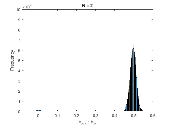
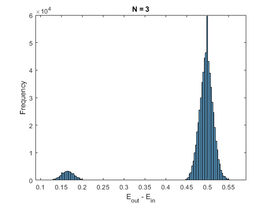
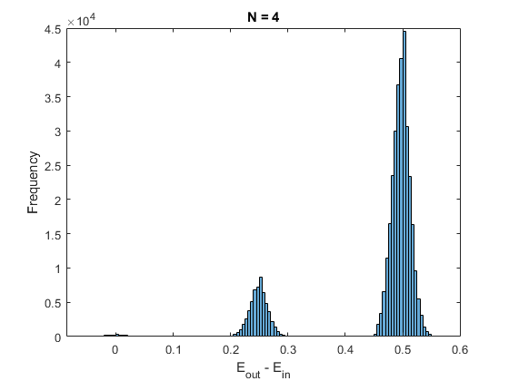
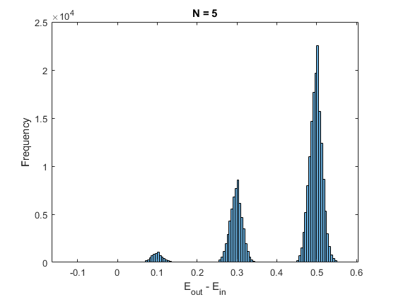
Since we are attempting to approximate randomly generated Boolean functions $f$, the average value of $E_{\rm{out}}$ is going to be $0.5$. This is so because a randomly generated Boolean function can evaluate to $0$ or $1$ with equal probability at every input value. Therefore, the given experiment is not going to yield good approximations of $f$. This is fine as we are concerned with observing the connection between the in-sample and out-of-sample errors as the sample size $N$ increases.

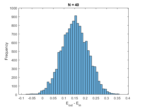
The results of the initial run of the experiment can are given in Figure 1. In the cases where the sample $N$ size is below $d_{\rm{vc}}=4$, it can be seen that $E_{\rm{out}}-E_{\rm{in}}$ is around $0.5$ for a vast number of cases, this is due to the fact that for small sample sizes, it is possible to find a large number of hypotheses with near-zero $E_{\rm{in}}$, but many of these hypotheses will invariably be poor approximations and therefore the in-sample error is a very poor generalization for the out-of-sample error.

This situation changes as we reach $N=4$, the (conjectured) VC dimension for this problem. There are now some situations where $E_{\rm{out}}-E_{\rm{in}}<0.5$. In these cases, $E_{\rm{in}}$ is a relatively better generalization of $E_{\rm{out}}$. This situation improves further as one moves beyond the VC dimension in $N=5$.

The result of the experiment for the larger values of $N$ are given in Figure 2, it can now be seen that lower values of $E_{\rm{out}}-E_{\rm{in}}$ are occurring with greater frequency. This enables us to establish confidence intervals for the difference between the two errors. This implies that we are in the regime of probably approximately correct (PAC) learning.

Therefore, one can state the probability for the accuracy of the estimate of the out-of-sample error with respect to $E_{\rm{in}}(g)$ for the functions belonging to ${\mathcal{H}}_{10}$. This serves as an elementary illustration that learning becomes feasible as the size of the sample $N$, increases beyond the VC dimension.

It should be noted that increasing the sample size after a point does not increase the overall accuracy of the approximation. This can be seen by reading off the values of the average in-sample error from Table 1 and observing the corresponding plot from Figure 1 or Figure 2.

Logical Analysis of Data (LAD) as proposed by Peter L. Hammer demonstrates significantly accurate results by fitting Boolean functions to the training set. However, we have not found any research on incorporating LAD into the PAC learning framework. We initiate such an effort in this article. We believe that research in this direction will help us in characterizing cases when LAD can be used as feasible learning algorithm. The methods presented here may also let us construct provably unlearnable Boolean functions.

References

- Hammer [1986] P.L. Hammer. Partially defined boolean functions and cause-effect relationships. In International Conference on Multi-attribute Decision Making Via OR-based Expert Systems. University of Passau, Passau, Germany, April 1986.
- Crama et al. [1988] Y. Crama, P.L. Hammer, and T. Ibaraki. Cause-effect relationships and partially defined boolean functions. Ann. Oper. Res., 16(1-4):299–325, January 1988. ISSN 0254-5330.
- Alexe et al. [2007] Gabriela Alexe, Sorin Alexe, Tibérius O. Bonates, and Alexander Kogan. Logical analysis of data – the vision of Peter L. Hammer. Annals of Mathematics and Artificial Intelligence, 49(1):265–312, Apr 2007. doi: 10.1007/s10472-007-9065-2. URL https://doi.org/10.1007/s10472-007-9065-2.
- Chauhan et al. [2022] Sneha Chauhan, Loreen Mahmoud, Sugata Gangopadhyay, and Aditi Kar Gangopadhyay. A comparative study of lad, CNN and DNN for detecting intrusions. In Hujun Yin, David Camacho, and Peter Tiño, editors, Intelligent Data Engineering and Automated Learning - IDEAL 2022 - 23rd International Conference, IDEAL 2022, Manchester, UK, November 24-26, 2022, Proceedings, volume 13756 of Lecture Notes in Computer Science, pages 443–455. Springer, 2022. doi: 10.1007/978-3-031-21753-1\_43. URL https://doi.org/10.1007/978-3-031-21753-1_43.
- Crama and Hammer [2011] Yves Crama and Peter L. Hammer. Boolean Functions - Theory, Algorithms, and Applications, volume 142 of Encyclopedia of mathematics and its applications. Cambridge University Press, 2011. ISBN 978-0-521-84751-3. URL http://www.cambridge.org/gb/knowledge/isbn/item6222210/?site_locale=en_GB.
- Boros et al. [2011] Endre Boros, Yves Crama, Peter L. Hammer, Toshihide Ibaraki, Alexander Kogan, and Kazuhisa Makino. Logical analysis of data: classification with justification. Ann. Oper. Res., 188(1):33–61, 2011. doi: 10.1007/s10479-011-0916-1. URL https://doi.org/10.1007/s10479-011-0916-1.
- Valiant [1984a] Leslie G. Valiant. A theory of the learnable. Commun. ACM, 27(11):1134–1142, 1984a. doi: 10.1145/1968.1972. URL https://doi.org/10.1145/1968.1972.
- Valiant [1984b] Leslie G. Valiant. A theory of the learnable. In Richard A. DeMillo, editor, Proceedings of the 16th Annual ACM Symposium on Theory of Computing, April 30 - May 2, 1984, Washington, DC, USA, pages 436–445. ACM, 1984b. doi: 10.1145/800057.808710. URL https://doi.org/10.1145/800057.808710.
- Abu-Mostafa et al. [2012] Yaser S. Abu-Mostafa, Malik Magdon-Ismail, and Hsuan-Tien Lin. Learning From Data. AMLBook, 2012. ISBN 1600490069.