Hierarchical Imitation Learning for Stochastic Environments

Learning to imitate behaviour is crucial when reward design is infeasible [1, 2, 3, 4], for overcoming hard exploration problems [5, 6], and for realistic modelling of dynamical systems with multiple interacting agents [7]. Such systems, including games, driving simulations, and agent-based economic models, often have known state transition functions, but require accurate agent models to be realistic. For example, for driving simulations, which are crucial for accelerating the development of autonomous vehicles [8, 9], faithful reactions of all road users are paramount. Furthermore, it is not enough to mimic a single mode in the data; instead, agents must reproduce the full distribution of behaviours to avoid sim2real gaps in modelled systems [10, 11].

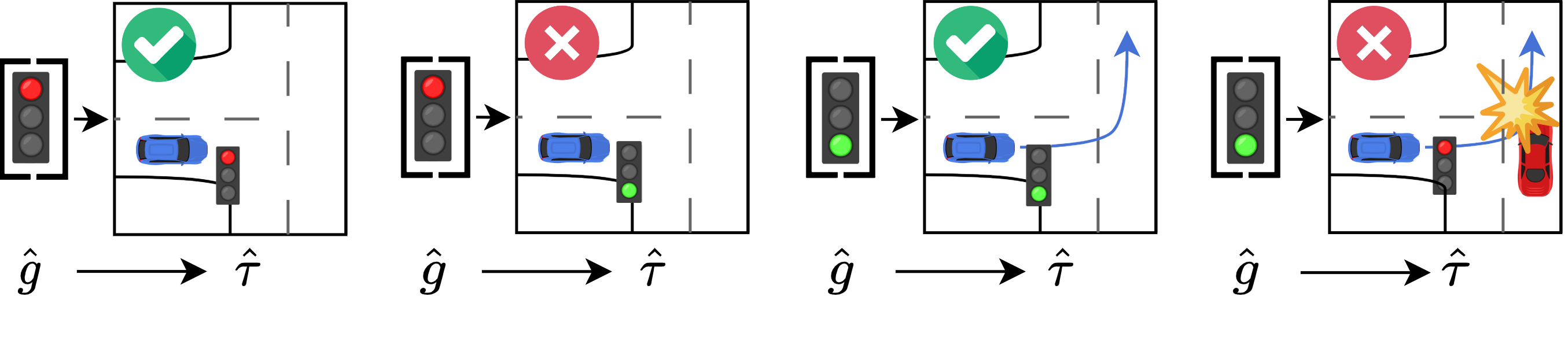
Current imitation learning (IL) methods fall short of achieving such distributional realism: while they are capable of generating individual trajectories that are realistic, they fail to match the full distribution of observed behaviour. Indeed, the adversarial training objective which enables state-of-the-art performance of most current IL methods is known to be prone to mode dropping in practice [12, 13, 14], even though it optimises a distribution-matching objective in principle [15, 16, 17]. Furthermore, progress on distributional realism is hindered by a lack of suitable benchmarks, with most relying on unimodal data and only evaluating task performance as measured by rewards, but not mode coverage or recall. By contrast, many applications, such as agent modeling for autonomous vehicles, require distributional realism in addition to good task performance. Consequently, our goal is to improve distributional realism while maintaining strong task performance.

To mitigate mode collapse and improve distributional realism in complex environments, previous work uses hierarchical policies in an autoencoder-like framework [12, 8, 9, 18]. During training, an encoder infers goals from observed future trajectories and the agent, conditioned on those goals, strives to imitate the original trajectory. At test time, a prior distribution proposes distributionally realistic goals, without requiring access to privileged future information. We refer to these goals as an agent’s inferred type since it can express not only goals, but many agent characteristics responsible for multi-modal behaviour, such as persona, goal, or strategy.

However, as we show in section III, using such hierarchical policies in stochastic environments can create a distribution shift between training and testing, possibly leading to out-of-distribution inputs and reduced performance. Unfortunately, the autoencoder training does not prevent extrinsic information from being encoded. Intuitively, the type should only capture agent-intrinsic choices that are under the agent’s control.

Consider a car waiting at an intersection (see fig. 1). During training, because the agent’s type (e.g., goal and driving style) are not directly observed, they must be inferred from its future trajectory. However, this inferred type might not only capture their goal and driving style, but also external factors out of the agent’s control, such as the time until the traffic light turns green. Even innocuous seeming type representations can leak external information; for example, a goal location extracted from the future trajectory can leak information about waiting times based on its distance to the starting position.

Capturing information about external events in the inferred type causes problems at test time, when the type must be sampled randomly without foresight of future events. For example, if the type contains information about traffic light timings, the actual timing on the test data will almost surely differ from the randomly sampled one, resulting in out-of-distribution inputs to the policy which never encountered such a mismatch during training where the type was always inferred from the actual future. Furthermore, the agent might have learned to ignore the actual traffic light, instead relying entirely on the inferred type that was always optimal during training. This could cause it to enter the intersection too early, resulting in potentially catastrophic consequences such as collisions.

Existing hierarchical work either assumes no external stochasticity in the environment [12, 8], relies on manually designed type representations that cannot capture external events but limit expressiveness [9], or relies on manually designed cost functions and type filters that mitigate the performance degradation but do not solve the underlying problem and induce biases in the learned behaviour [18].

In this paper, we identify the challenges arising under stochastic environments and formulate them as a new form of distribution shift for hierarchical policies. Unlike the familiar covariate shift in the state distribution [19], this conditional type shift occurs in the distribution of the inferred latent type. It greatly reduces performance by yielding causally confused agents that rely on the latent type for information about external factors, instead of inferring them from the latest environment observation. We propose Robust Type Conditioning (RTC) to eliminate this distribution shift through a coupled adversarial training objective under randomly sampled types. We do not require access to an expert, counterfactuals, or manually specified type labels for trajectories.

Experimentally, we show the need for improved distributional realism in state-of-the-art imitation learning techniques such as GAIL [16]. Furthermore, we show that naively trained hierarchical models with inferred types improve distributional realism, but exhibit poor task performance in stochastic environments. By contrast, RTC can maintain good task performance in stochastic environments while improving distributional realism. We evaluate RTC on the illustrative Double Goal Problem as well as the large scale Waymo Open Motion Dataset [20] of real driving behaviour.

We are given a dataset $\mathcal{D}=\{\tau_{i}\}_{i=1}^{N}$ of $N$ trajectories $\tau_{i}=\boldsymbol{s}_{0}^{(i)},\boldsymbol{a}_{0}^{(i)},\dots\boldsymbol{s}_{T}^{(i)}$, drawn from $p(\tau)$ of one or more experts interacting with a stochastic environment $p(\boldsymbol{s}_{t+1}|\boldsymbol{s}_{t},\boldsymbol{a}_{t})$ where $\boldsymbol{s}_{t}\in\mathcal{S}$ are states and $\boldsymbol{a}_{t}\in\mathcal{A}$ are actions. Our goal is to learn a policy $\boldsymbol{\pi}_{\boldsymbol{\theta}}(\boldsymbol{a}_{t}|\boldsymbol{s}_{t})$ to match $p(\tau)$ when replacing the unknown expert and generating rollouts $\hat{\tau}\sim p(\hat{\tau})=p(\boldsymbol{s}_{0})\prod_{t=0}^{T-1}\boldsymbol{\pi}_{\boldsymbol{\theta}}(\boldsymbol{\hat{a}}_{t}|\boldsymbol{\hat{s}}_{t})p(\boldsymbol{\hat{s}}_{t+1}|\boldsymbol{\hat{s}}_{t},\boldsymbol{\hat{a}}_{t})$ from the inital states $\boldsymbol{s}_{0}\sim p(\boldsymbol{s}_{0})$. We simplify notation and write $\hat{\tau}\sim\boldsymbol{\pi}_{\boldsymbol{\theta}}(\hat{\tau})$ and $\tau\sim\mathcal{D}(\tau)$ to indicate rollouts generated by the policy or drawn from the data respectively. Expectations $\mathbb{E}_{\tau\sim\mathcal{D}}$ and $\mathbb{E}_{\hat{\tau}\sim\boldsymbol{\pi}_{\boldsymbol{\theta}}}$ are taken over all pairs $(\boldsymbol{s}_{t},\boldsymbol{a}_{t})\in\tau$ and $(\boldsymbol{\hat{s}}_{t},\boldsymbol{\hat{a}}_{t})\in\hat{\tau}$.

Previous work [19, 16, e.g.,] shows that a core challenge of learning from demonstration is reducing or eliminating the covariate shift in the state-visitation frequencies $p(\boldsymbol{s})$ caused by accumulating errors when using $\boldsymbol{\pi}_{\boldsymbol{\theta}}$. Unfortunately, Behavioural Cloning (BC), a simple supervised training objective optimising $\max_{\boldsymbol{\theta}}\mathbb{E}_{\tau\sim\mathcal{D}}\left[\log\boldsymbol{\pi}_{\boldsymbol{\theta}}(\boldsymbol{a}_{t}|\boldsymbol{s}_{t})\right]$ is not robust to it. To overcome covariate shift, generative adversarial imitation learning (GAIL) [16] optimises $\boldsymbol{\pi}_{\boldsymbol{\theta}}$ to fool a learned discriminator $D_{\boldsymbol{\phi}}(\boldsymbol{\hat{a}}_{t},\boldsymbol{\hat{s}}_{t})$ that is trained to distinguish between trajectories in $\mathcal{D}$ and those generated by $\boldsymbol{\pi}_{\boldsymbol{\theta}}$:

The policy can be optimised using reinforcement learning, by treating the log-discriminator scores as costs, $r_{t}=-\log D_{\boldsymbol{\phi}}(\boldsymbol{\hat{a}}_{t},\boldsymbol{\hat{s}}_{t})$. Alternatively, if the policy can be reparameterized [21] and the environment is differentiable, the sum of log discriminator scores can be optimised directly without relying on high-variance score function estimators by backpropagating through the transition dynamics, $\mathcal{L}_{\text{adv}}(\hat{\tau})=\mathbb{E}_{\hat{\tau}\sim\boldsymbol{\pi}_{\boldsymbol{\theta}}}\left[\sum_{t}-\log D_{\boldsymbol{\phi}}(\boldsymbol{\hat{a}}_{t},\boldsymbol{\hat{s}}_{t})\right]$. We refer to this as Model-based GAIL (MGAIL) and assume a known differentiable environment instead of a learned model as in [17].

In this work, we are concerned with multimodal distributions $p(\tau)$ and how mode collapse can be avoided when learning $\boldsymbol{\pi}_{\boldsymbol{\theta}}$. To this end, we assume the dataset is sampled from $p(\tau)=p(\boldsymbol{s}_{0})\int p(\boldsymbol{g})p(\boldsymbol{\xi})\prod_{t=0}^{T}p(\boldsymbol{a}_{t}|\boldsymbol{s}_{t},\boldsymbol{g})p(\boldsymbol{s}_{t+1}|\boldsymbol{s}_{t},\boldsymbol{a}_{t},\boldsymbol{\xi})d\boldsymbol{\xi}d\boldsymbol{g}$, where $\boldsymbol{g}$ is the agent type, expressing agent characteristics such as persona, goal, or, strategy, and $\boldsymbol{\xi}$ is a random variable capturing the stochasticity in the environment, i.e., $p(\boldsymbol{s}_{t+1}|\boldsymbol{s}_{t},\boldsymbol{a}_{t},\boldsymbol{\xi})$ is a delta distribution $\delta_{f(\boldsymbol{s}_{t},\boldsymbol{a}_{t},\boldsymbol{\xi})}(s_{t+1})$ for some transition function $f$. We call an agent realistic if its generated trajectories $\hat{\tau}\sim\boldsymbol{\pi}_{\boldsymbol{\theta}}$ lie in the support of $p(\tau)$. We call an agent distributionally realistic if its distribution over trajectories matches the data, i.e. $p(\hat{\tau})\approx p(\tau)$. As we show in section VI, current non-hierarchical adversarial methods [16] are not distributionally realistic.

To combat mode collapse, hierarchical methods [12, 22, 8, 9, 18, e.g.,] often rely on an encoder to infer latent agent types $\boldsymbol{\hat{g}}_{e}$ from trajectories during training, $\boldsymbol{\hat{g}_{e}}\sim\boldsymbol{e}_{\boldsymbol{\theta}}(\boldsymbol{\hat{g}}_{e}|\tau)$, and optimise the control policy $\boldsymbol{\pi}_{\boldsymbol{\theta}}(\boldsymbol{\hat{a}}_{t}|\boldsymbol{\hat{s}}_{t},\boldsymbol{\hat{g}}_{e})$ to generate trajectories $\hat{\tau}_{e}$ similar to $\tau$: $\hat{\tau}_{e}\sim p(\hat{\tau}_{e}|\boldsymbol{\hat{g}}_{e})=p(\boldsymbol{s}_{0})\prod_{t=0}^{T-1}\boldsymbol{\pi}_{\boldsymbol{\theta}}(\boldsymbol{\hat{a}}_{t}|\boldsymbol{\hat{s}}_{t},\boldsymbol{\hat{g}}_{e})p(\boldsymbol{\hat{s}}_{t+1}|\boldsymbol{\hat{a}}_{t},\boldsymbol{\hat{s}}_{t})$. As ground truth trajectories are not accessible during testing, a prior $p_{\boldsymbol{\theta}}(\boldsymbol{\hat{g}}_{p})$, which has been trained to match the marginal distribution $p_{e}(\boldsymbol{\hat{g}}_{e})=\mathbb{E}_{\tau}\left[\boldsymbol{e}_{\boldsymbol{\theta}}(\boldsymbol{\hat{g}}_{e}|\tau)\right]$, is used to sample distributionally realistic types $\boldsymbol{\hat{g}}_{p}$. We indicate by subscript $\boldsymbol{\hat{g}}_{p}$ or $\boldsymbol{\hat{g}}_{e}$ whether the inferred type and trajectory are drawn from the prior distribution $p_{\boldsymbol{\theta}}(\boldsymbol{\hat{g}}_{p})$ or encoder $\boldsymbol{e}_{\boldsymbol{\theta}}(\boldsymbol{\hat{g}}_{e}|\tau)$. Subscripts are omitted for states and actions to simplify notation. Inferred types and predicted trajectories without subscripts indicate that either sampling distribution could be used. For information theoretic quantities we use capital letters ${S},{A},{\hat{A}},{\hat{G}}$ and ${\Xi}$ to denote the random variables for values $\boldsymbol{s},\boldsymbol{a},\boldsymbol{\hat{a}},\boldsymbol{\hat{g}}$ and $\boldsymbol{\xi}$.

Here we outline the challenge of conditional type shift that arises for hierarchical policies in stochastic environments. We provide a simple example illustrating the challenge and how it can be overcome, as well as formulate a proof for the exact conditions under which such a distribution shift occurs. These insights motivate the algorithm in section IV.

We present Robust Type Conditioning (RTC), a method for improving distributional realism in imitation learning while maintaining high task performance, even in stochastic environments. As shown in previous work [8, 9, 18], and confirmed in section VI, hierarchical policies trained in an autoencoder framework are currently the most effective approach at improving distributional realism. However, such policies require the latent type to be inferred from the future trajectory, which can cause problems in stochastic environments (see section III).

To overcome this limitation, we propose to combine the autoencoder training objective $\mathcal{L}_{\text{vae}}=\mathcal{L}_{\text{rec}}+\beta\mathcal{L}_{\text{kl}}$ with an additional adversarial objective $\mathcal{L}_{\text{adv}}$ utilising a learned discriminator $D_{\boldsymbol{\phi}}(\boldsymbol{a}_{t},\boldsymbol{s}_{t})$. Importantly, this additional objective allows us to sample training types not only from the encoder, but also from the prior. When types are sampled from the prior, the hierarchical loss $\mathcal{L}_{\text{vae}}$ cannot be used as we generally do not have access to ground truth trajectories corresponding to this specific type, which are required for the reconstruction loss $\mathcal{L}_{\text{rec}}$. Instead, for these types, we only optimise the adversarial objective $\mathcal{L}_{\text{adv}}(\hat{\tau})=\sum_{t}-\log D_{\boldsymbol{\phi}}(\boldsymbol{\hat{a}}_{t},\boldsymbol{\hat{s}}_{t})$.

During training, we hence split each minibatch $\mathcal{B}=\{\tau^{(b)}\}_{b}^{N_{b}}$ of $N_{b}$ trajectories sampled from $\mathcal{D}$ into two parts. For the fraction $f$ of trajectories in $\mathcal{B}_{\text{}}$ the rollouts $\hat{\tau}_{e}$ are generated from types sampled from the encoder $\boldsymbol{\hat{g}}_{e}\sim\boldsymbol{e}_{\boldsymbol{\theta}}(\boldsymbol{\hat{g}}_{e}|\tau)$ and objectives $\mathcal{L}_{\text{adv}}+\lambda\mathcal{L}_{\text{vae}}$ are optimised (first line in eq. 4). For the remaining fraction $(1-f)$ of trajectories, types are sampled from the prior $p_{\boldsymbol{\theta}}(\boldsymbol{\hat{g}}_{p})$ and only $\mathcal{L}_{\text{adv}}$ is optimised (second line in eq. 4).

Because the policy does not know whether the type is sampled from the encoder or prior, this combination ensures that policies follow agent-internal information in the type, due to the autoencoder training objective, but ignore any information in the type about external stochastic events, as this would lead to unrealistic trajectories under prior types, which are penalised by the adversarial training objective. Lastly, because the KL objective $\mathcal{L}_{\text{kl}}(\tau)=\mathbb{E}_{\tau\sim\mathcal{D}}\left[\KL\left[p_{\boldsymbol{\theta}}(\boldsymbol{\hat{g}}_{p})\|\boldsymbol{e}_{\boldsymbol{\theta}}(\boldsymbol{\hat{g}}_{e}|\tau)\right]\right]$ minimises the amount of information encoded in the type, such unused information would not even be encoded.

Consequently, the full RTC loss is

with

where $p_{\boldsymbol{\theta}}(\boldsymbol{\hat{g}}_{p})$ is a learned prior, $\boldsymbol{e}_{\boldsymbol{\theta}}(\boldsymbol{\hat{g}}_{e}|\tau)$ a learned trajectory encoder and $\boldsymbol{\pi}_{\boldsymbol{\theta}}(\hat{\tau}|\boldsymbol{\hat{g}})$ is shorthand for generating trajectories $\hat{\tau}$ by rolling out the learned control policy $\boldsymbol{\pi}_{\boldsymbol{\theta}}(\boldsymbol{\hat{a}}|\boldsymbol{\hat{s}},\boldsymbol{\hat{g}})$ in the environment. Parameters $\boldsymbol{\bar{\theta}}$ are held fixed and $\lambda$ and $\beta$ are scalar weights. $D_{\boldsymbol{\phi}}(\boldsymbol{a}_{t},\boldsymbol{s}_{t})$ is a learned per-timestep discriminator. Lastly, $\mathcal{L}_{\text{rec}}(\tau,\hat{\tau})$ is a reconstruction loss between $\tau$ and $\hat{\tau}_{e}$ which can take different forms. For example, in section VI-A we use the BC loss $\mathcal{L}_{\text{rec}}(\tau,\hat{\tau})=-\log\boldsymbol{\pi}_{\boldsymbol{\theta}}(\boldsymbol{a}_{t}|\boldsymbol{s}_{t},\boldsymbol{\hat{g}}_{e})$ while in section VI-B we minimise the $L_{2}$ distance between agent positions in $\boldsymbol{s}_{t}$ and $\boldsymbol{\hat{s}}_{t}$. The loss $\mathcal{L}_{\text{kl}}(\tau)$ optimises the prior to propose distributionally realistic types by matching the marginal encoder distribution.

One can understand the problem of conditional type shift as one of causally confused policies which refer to the type for information about external stochastic events, instead of acquiring this information directly from the currently observed states. From this perspective, sampling from the prior constitutes a causal intervention $do(\boldsymbol{\hat{g}})$ in which $\boldsymbol{\hat{g}}$ is changed independently of the environmental factor $\boldsymbol{\xi}$. [23] show that causal confusion can be avoided by applying such interventions and optimising the policy to correctly predict the counterfactual expert trajectory distribution, in our case $p_{\text{expert}}(\tau|\boldsymbol{\xi},do(\boldsymbol{\hat{g}}))$. Unfortunately, we do not have access to this counterfactual trajectory. Instead, we rely on the generalisation of $\boldsymbol{\pi}_{\boldsymbol{\theta}}$ to get us ‘close’ to such a counterfactual trajectory for types $do(\boldsymbol{\hat{g}})$ and then refine the policy locally using the adversarial objective.

We find that both continuous type representations with and discrete type representations using straight-through gradient estimation work well in practice (see section VI-B).

Optimisation of $\mathcal{L}_{\text{adv}}$ and $\mathcal{L}_{\text{rec}}$ can either be performed directly, similar to MGAIL [17], by using a differentiable environment and reparameterised policies and encoder [21] or by treating them as rewards and using RL methods such as TRPO [24, 16] or PPO [25]. The loss $\mathcal{L}_{\text{kl}}$ can always be optimised directly.

Hierarchical policies have been extensively studied in RL [26, 27, 28, 29, 30, e.g.,] and IL. In RL, they improve exploration, sample efficiency and fast adaptation. By contrast, in IL, hierarchies are used to capture multimodal distributions, improve data efficiency [31, 32], and enable goal conditioning [33]. Similar to our work, [12] and [22] learn to encode trajectories into latent types that influence a control policy. Crucially, both only consider deterministic environments and hence avoid the distribution shifts and unwanted information leakage we address. They extend prior work in which the type, or context, is provided in the dataset [34], which is also assumed in [35]. [36] use a sampling method to infer latent types. [37] and [9] use manually designed encoders specific to road users by expressing future goals as sequences of lane segments. This avoids information leakage but cannot express all characteristics of human drivers, such as persona, and cannot transfer to other tasks. BITS [18] uses goal positions as types, which suffer from conditional type shift. Consequently, their method requires behaviour prediction and a manually specified cost function to filter goals that might mismatch with predicted futures. Futures states in deterministic environments [38], language [39], and predefined strategy statistics [40] have also been used as types.

Information theoretic regularization offers an alternative to learning hierarchical policies using the auto-encoder framework [41, 42]. However, these methods are less expressive since their prior distribution cannot be learned and only aim to cluster modes already captured by the agent but not penalize dropping modes in the data. This provides a useful inductive bias but often struggles in complex environments with high diversity, requiring manual feature engineering [43, 44].

Lastly, TrafficSim [8] uses IL to model driving agents, controlling all stochasticity in the scene but using independent prior distributions for separate agents. Hence, while the environment is assumed deterministic, conditional type shift can occur between the separate agent-types which are correlated during training but independent during testing. They use a biased “common sense” collision avoidance loss, motivated by covariate shift in visited states. Our work suggests that type shift might also explain the benefits gained. In contrast, our adversarial objective is unbiased.

We show in two stochastic environments with multimodal expert behaviour that i) existing IL methods suffer from insufficient distributional realism, ii) hierarchical methods can suffer from conditional type shift and degrading task performance, and iii) RTC improves distributional realism while maintaining excellent task performance.

We compare the following models: MGAIL uses an adversarial training objective with learned discriminator. It also optimises a BC loss as we found this to improve performance. Symphony [9] (called ‘MGAIL+H’ in the original paper), building on MGAIL, utilises future lane segments as manually specified types which avoid conditional type shift but limit expressiveness. InfoMGAIL [41] augments MGAIL to elicit distinct trajectories for different types by using an information-theoretic loss. This is an alternative training paradigm for hierarchical policies, besides using autoencoders with reconstruction loss. For fair comparison, our method RTC uses the same MGAIL implementation as adversarial objective. We investigate both continuous and discrete type representations, RTC-C and RTC-D. NaiveHierarchy is a hierarchical autoencoder not training on prior-sampled types (but also using the adversarial MGAIL objective) and hence experiencing conditional type shift and high collision frequency.

This paper identified new challenges in learning hierarchical policies from demonstration to capture multimodal trajectory distributions in stochastic environments. We expressed them as conditional type shifts in the hierarchical policy. We proposed Robust Type Conditioning (RTC) to eliminate these distribution shifts and showed improved distributional realism while maintaining or improving task performance on two stochastic environments, including the Waymo Open Motion Dataset [20]. Future work will address conditional distributional realism by not only matching the marginal distribution $p(\tau)$, but the conditional distribution $p(\tau|\boldsymbol{\xi})$ under a specific realization of the environment. For example, drivers might change their intent based on the current traffic situation or players might adapt their strategy as the game unfolds. Achieving such conditional distributional realism will also require new models and metrics.

References

- [1] D. Amodei, C. Olah, J. Steinhardt, P. Christiano, J. Schulman, and D. Mané, “Concrete problems in ai safety,” arXiv preprint arXiv:1606.06565, 2016.
- [2] D. Hadfield-Menell, S. Milli, P. Abbeel, S. J. Russell, and A. Dragan, “Inverse reward design,” Advances in neural information processing systems, vol. 30, 2017.
- [3] J. Fu, K. Luo, and S. Levine, “Learning robust rewards with adverserial inverse reinforcement learning,” in International Conference on Learning Representations, 2018. [Online]. Available: https://openreview.net/forum?id=rkHywl-A-
- [4] T. Everitt, M. Hutter, R. Kumar, and V. Krakovna, “Reward tampering problems and solutions in reinforcement learning: A causal influence diagram perspective,” Synthese, vol. 198, no. 27, pp. 6435–6467, 2021.
- [5] A. Rajeswaran, V. Kumar, A. Gupta, G. Vezzani, J. Schulman, E. Todorov, and S. Levine, “Learning complex dexterous manipulation with deep reinforcement learning and demonstrations,” arXiv preprint arXiv:1709.10087, 2017.
- [6] Y. Zhu, Z. Wang, J. Merel, A. Rusu, T. Erez, S. Cabi, S. Tunyasuvunakool, J. Kramár, R. Hadsell, N. de Freitas et al., “Reinforcement and imitation learning for diverse visuomotor skills,” arXiv preprint arXiv:1802.09564, 2018.
- [7] J. D. Farmer and D. Foley, “The economy needs agent-based modelling,” Nature, vol. 460, no. 7256, pp. 685–686, 2009.
- [8] S. Suo, S. Regalado, S. Casas, and R. Urtasun, “Trafficsim: Learning to simulate realistic multi-agent behaviors,” in ICCV, 2021.
- [9] M. Igl, D. Kim, A. Kuefler, P. Mougin, P. Shah, K. Shiarlis, D. Anguelov, M. Palatucci, B. White, and S. Whiteson, “Symphony: Learning realistic and diverse agents for autonomous driving simulation,” in ICRA, 2022.
- [10] A. Grover, M. Al-Shedivat, J. Gupta, Y. Burda, and H. Edwards, “Learning policy representations in multiagent systems,” in International conference on machine learning. PMLR, 2018, pp. 1802–1811.
- [11] Y. Liang, C. Guo, Z. Ding, and H. Hua, “Agent-based modeling in electricity market using deep deterministic policy gradient algorithm,” IEEE Transactions on Power Systems, vol. 35, no. 6, 2020.
- [12] Z. Wang, J. S. Merel, S. E. Reed, N. de Freitas, G. Wayne, and N. Heess, “Robust imitation of diverse behaviors,” NeurIPS, 2017.
- [13] M. Lucic, K. Kurach, M. Michalski, S. Gelly, and O. Bousquet, “Are gans created equal? a large-scale study,” NeurIPS, 2018.
- [14] A. Creswell, T. White, V. Dumoulin, K. Arulkumaran, B. Sengupta, and A. A. Bharath, “Generative adversarial networks: An overview,” IEEE signal processing magazine, vol. 35, no. 1, pp. 53–65, 2018.
- [15] I. Goodfellow, J. Pouget-Abadie, M. Mirza, B. Xu, D. Warde-Farley, S. Ozair, A. Courville, and Y. Bengio, “Generative adversarial networks,” Communications of the ACM, vol. 63, no. 11, pp. 139–144, 2020.
- [16] J. Ho and S. Ermon, “Generative adversarial imitation learning,” NeurIPS, 2016.
- [17] N. Baram, O. Anschel, and S. Mannor, “Model-based adversarial imitation learning,” arXiv preprint arXiv:1612.02179, 2016.
- [18] D. Xu, Y. Chen, B. Ivanovic, and M. Pavone, “Bits: Bi-level imitation for traffic simulation,” arXiv preprint arXiv:2208.12403, 2022.
- [19] S. Ross, G. Gordon, and D. Bagnell, “A reduction of imitation learning and structured prediction to no-regret online learning.” JMLR Workshop and Conference Proceedings, 2011.
- [20] S. Ettinger, S. Cheng, B. Caine, C. Liu, H. Zhao, S. Pradhan, Y. Chai, B. Sapp, C. Qi, Y. Zhou, Z. Yang, A. Chouard, P. Sun, J. Ngiam, V. Vasudevan, A. McCauley, J. Shlens, and D. Anguelov, “Large scale interactive motion forecasting for autonomous driving : The waymo open motion dataset,” CoRR, 2021.
- [21] D. P. Kingma and M. Welling, “Auto-encoding variational bayes,” ICLR, 2014.
- [22] C. Lynch, M. Khansari, T. Xiao, V. Kumar, J. Tompson, S. Levine, and P. Sermanet, “Learning latent plans from play,” in Conference on robot learning. PMLR, 2020, pp. 1113–1132.
- [23] P. De Haan, D. Jayaraman, and S. Levine, “Causal confusion in imitation learning,” NeurIPS, 2019.
- [24] J. Schulman, S. Levine, P. Abbeel, M. Jordan, and P. Moritz, “Trust region policy optimization,” in ICML, 2015.
- [25] J. Schulman, F. Wolski, P. Dhariwal, A. Radford, and O. Klimov, “Proximal policy optimization algorithms,” arXiv:1707.06347, 2017.
- [26] R. S. Sutton, D. Precup, and S. Singh, “Between mdps and semi-mdps: A framework for temporal abstraction in reinforcement learning,” Artificial intelligence, vol. 112, no. 1-2, pp. 181–211, 1999.
- [27] P.-L. Bacon, J. Harb, and D. Precup, “The option-critic architecture,” in AAAI, 2017.
- [28] A. S. Vezhnevets, S. Osindero, T. Schaul, N. Heess, M. Jaderberg, D. Silver, and K. Kavukcuoglu, “Feudal networks for hierarchical reinforcement learning,” in ICML, 2017.
- [29] O. Nachum, S. Gu, H. Lee, and S. Levine, “Near-optimal representation learning for hierarchical reinforcement learning,” in ICLR, 2019.
- [30] M. Igl, A. Gambardella, J. He, N. Nardelli, N. Siddharth, W. Böhmer, and S. Whiteson, “Multitask soft option learning,” in UCA, 2020.
- [31] S. Krishnan, R. Fox, I. Stoica, and K. Goldberg, “Ddco: Discovery of deep continuous options for robot learning from demonstrations,” in Conference on robot learning. PMLR, 2017, pp. 418–437.
- [32] H. Le, N. Jiang, A. Agarwal, M. Dudik, Y. Yue, and H. Daumé III, “Hierarchical imitation and reinforcement learning,” in ICML, 2018.
- [33] K. Shiarlis, M. Wulfmeier, S. Salter, S. Whiteson, and I. Posner, “Taco: Learning task decomposition via temporal alignment for control,” in ICML, 2018.
- [34] J. Merel, Y. Tassa, D. TB, S. Srinivasan, J. Lemmon, Z. Wang, G. Wayne, and N. Heess, “Learning human behaviors from motion capture by adversarial imitation,” arXiv:1707.02201, 2017.
- [35] C. Fei, B. Wang, Y. Zhuang, Z. Zhang, J. Hao, H. Zhang, X. Ji, and W. Liu, “Triple-gail: a multi-modal imitation learning framework with generative adversarial nets,” arXiv preprint arXiv:2005.10622, 2020.
- [36] A. Tamar, K. Rohanimanesh, Y. Chow, C. Vigorito, B. Goodrich, M. Kahane, and D. Pridmore, “Imitation learning from visual data with multiple intentions,” in ICLR, 2018.
- [37] S. Khandelwal, W. Qi, J. Singh, A. Hartnett, and D. Ramanan, “What-if motion prediction for autonomous driving,” arXiv preprint arXiv:2008.10587, 2020.
- [38] Y. Ding, C. Florensa, P. Abbeel, and M. Phielipp, “Goal-conditioned imitation learning,” NeurIPS, 2019.
- [39] A. Pashevich, C. Schmid, and C. Sun, “Episodic transformer for vision-and-language navigation,” in ICCV, 2021.
- [40] O. Vinyals, I. Babuschkin, W. M. Czarnecki, M. Mathieu, A. Dudzik, J. Chung, D. H. Choi, R. Powell, T. Ewalds, P. Georgiev et al., “Grandmaster level in starcraft ii using multi-agent reinforcement learning,” Nature, vol. 575, no. 7782, pp. 350–354, 2019.
- [41] Y. Li, J. Song, and S. Ermon, “Infogail: Interpretable imitation learning from visual demonstrations,” Advances in Neural Information Processing Systems, vol. 30, 2017.
- [42] K. Hausman, Y. Chebotar, S. Schaal, G. Sukhatme, and J. J. Lim, “Multi-modal imitation learning from unstructured demonstrations using generative adversarial nets,” in NeurIPS, 2017.
- [43] B. Eysenbach, A. Gupta, J. Ibarz, and S. Levine, “Diversity is all you need: Learning skills without a reward function,” in ICLR, 2019.
- [44] D. Pathak, D. Gandhi, and A. Gupta, “Self-supervised exploration via disagreement,” in ICML, 2019.