Neural Stochastic Screened Poisson ReconstructionCCS: Computing methodologies Point-based modelsCCS: Computing methodologies 3D imagingCCS: Computing methodologies Active visionCCS: Computing methodologies Uncertainty quantificationConference: SIGGRAPH Asia 2023 Conference Papers; December 12–15, 2023; Sydney, NSW, AustraliaSIGGRAPH Asia 2023 Conference Papers (SA Conference Papers ’23), December 12–15, 2023, Sydney, NSW, AustraliaPrice: 15.00DOI: 10.1145/3610548.3618162ISBN: 979-8-4007-0315-7/23/12

Abstract.
Reconstructing a surface from a point cloud is an underdetermined problem. We use a neural network to study and quantify this reconstruction uncertainty under a Poisson smoothness prior. Our algorithm addresses the main limitations of existing work and can be fully integrated into the 3D scanning pipeline, from obtaining an initial reconstruction to deciding on the next best sensor position and updating the reconstruction upon capturing more data.
Keywords:
neural surface reconstruction, uncertainty quantification1. Introduction


Surface reconstruction is the process of transforming a discrete set of points in space (a common format for captured 3D geometry) into a complete two-dimensional manifold for use in downstream scientific applications. Given the fundamentally underdetermined nature of the problem, algorithms must rely on priors to decide on an output surface.
Absent task-specific knowledge, the predominant geometry processing algorithm for surface reconstruction is Poisson Surface Reconstruction (PSR) [Kazhdan et al. 2006]. PSR encourages smoothness in the reconstruction through a Partial Differential Equation (PDE) whose solution can be computed efficiently and robustly. Drawing inspiration from it, Dai and Nießner 2022 recently introduced a neural approximation of PSR, which sidesteps the PDE perspective on the problem, achieving some performance gains at the cost of losing theoretical guarantees (see Figure 4), overfitting (see Figure 3) and additional requirements (e.g., sensor positioning).
Statistically, PSR generates the most probable reconstruction based on the selected prior. This choice inherently defines an entire posterior distribution in the space of possible reconstructions. While Stochastic PSR [Sellán and Jacobson 2022] computes this distribution for the first time in the context of PSR, it demands a complex discretization scheme and relies on multiple approximations to achieve computational tractability.
We build on the work by Sellán and Jacobson 2022 and introduce a neural formulation of Stochastic PSR that provides a full statistical formalism of the reconstruction process while avoiding overfitting and requiring no additional sensor information. Unlike Sellán and Jacobson 2022, we parametrize the mean and covariance of the implicit field describing the reconstructed surface using a neural network (see Figure 2), which we optimize using gradient-based optimization on losses derived from the variational version of the Poisson equation. Our neural formulation also allows us to extend this stochastic perspective beyond the original PSR and into Screened PSR [Kazhdan and Hoppe 2013].
We showcase the power of our algorithm by showing its performance in a breadth of applications made possible by our novel neural perspective. In particular, we show how one can fully integrate our algorithm in the 3D scanning pipeline, from obtaining an initial reconstruction to defining a differential camera score that can guide the choice of the next best scanning position and efficiently updating the previous reconstruction (see Figure 1) by fine-tuning our network with additional data. We also explore promising avenues for future work, like latent space generalization over scanning positions for a given object or over a space of objects.
2. Related Work
2.1. Surface reconstruction
Three-dimensional geometry is often captured by recording the distance from a sensor or depth camera to a real-world object [Raj et al. 2020; Özyeşil et al. 2017]. Combining the information from many sensors allows us to represent the raw captured geometry as a discrete set of points in space or point cloud. It is often possible to use properties about the sensor positioning or heuristics based on global or local cloud attributes [Hoppe et al. 1992; König and Gumhold 2009; Schertler et al. 2017; Metzer et al. 2021] to equip every point with a normal direction, allow for the slightly more complete representation of an oriented point cloud.
Despite their ubiquitousness, (oriented) point clouds are a fundamentally underdetermined surface representation: by specifying only a discrete set of points in space through which a surface passes, it describes a theoretically infinite number of possible surfaces. Surface Reconstruction algorithms (see [Berger et al. 2017] for a survey) use a prior to decide between them and output a fully determined surface, usually in a format appropriate for specific downstream tasks like a mesh or an implicit function. These priors range from simple geometric primitives [Schnabel et al. 2009] to global properties like symmetry [Pauly et al. 2008] or self-similarity [Williams et al. 2019], user-specified ones [Sharf et al. 2007] and, especially in recent years, data-driven [Remil et al. 2017; Groueix et al. 2018].
Absent task-specific knowledge, a commonly used prior is smoothness. This can be enforced explicitly by considering only surfaces parametrized by a smooth family of functions; for example, spatially-varying polynomials [Levin 2004; Alexa et al. 2003; Ohtake et al. 2005] and linear combinations of radial basis functions [Carr et al. 2001]. Smoothness can also be enforced variationally: Poisson Surface Reconstruction (PSR) [Kazhdan et al. 2006; Kazhdan and Hoppe 2013] encodes volumetric smoothness away from the input point cloud by minimizing the integrated gradient of the surface’s implicit representation and remains one of the best performing general surface reconstruction algorithms in terms of robustness and efficiency (see Table 1 in [Berger et al. 2017]). While the authors solve this optimization problem using the Finite Element Method on a hierarchical grid, Dai and Nießner 2022 have recently proposed using a neural network for a similar task, albeit they suggest forgoeing the volumetric integration and instead minimizing the gradient only at the point cloud points (see Figs. 3 and 4). We cover PSR and its variants in more detail in Section 3.1.
2.2. Stochastic Surface Reconstruction
From a statistical perspective, the vast majority of surface reconstruction works limit themselves to outputting the likeliest surface given the point cloud observations and their assumed prior. Relatively fewer works take this stochastic perspective one step further and compute a posterior distribution of all possible surfaces conditioned on the observations. For example, Pauly et al. 2004 quantify the likelihood of any spatial point belonging to the reconstructed surface by measuring its alignment with the point cloud.
More recently, Stochastic Poisson Surface Reconstruction [Sellán and Jacobson 2022] reinterprets the classic algorithm as a Gaussian Process, enabling the computation of statistical queries crucial to the reconstruction process and applications such as ray casting, point cloud repair, and collision detection. The authors utilize a Finite Element discretization to compute the mean and covariance functions of the posterior multivariate Gaussian distribution, which represents the likelihood of all possible reconstructions (see Section 3.2), resorting to a several approximations and parameter choices for computational tractability (see Figure 5). In contrast, our work proposes the parametrization of these functions using neural networks, optimizing them through gradient-based methods for a more efficient and flexible approach while still computing the same statistical quantities (see Figure 7).
2.3. Neural PDE solvers
We propose solving the Poisson equation in Stochastic PSR using a neural network. As such, our algorithm is one more application in the growing field of neural partial differential equation solvers. A broad class of these are Physics-Informed Neural Networks (PINNs) (see [Cuomo et al. 2022] for a literature review), which effectively soften a PDE and its boundary conditions into integral loss terms that are minimized with, e.g., stochastic gradient descent.
If a given PDE accepts a variational formulation, the above process can be done in a more principled way, as shown by Yu et al. 2018. This is the case for the Poisson equation, which can be equivalently described as a variational Dirichlet energy minimization. This is noted by Sitzmann et al. 2020, who show the impressive performance of sinusoidal activation functions when applied to Dirichlet-type problems. We borrow from their observations and propose a network architecture with sine activations.

2.4. Next-Best-View planning
A key benefit of proposed approach is its integration in the 3D scanning process. Specifically, it allows us to compute a score function that quantifies how useful a proposed next sensor position would be for the reconstruction task. This is a common first step in the active vision or next-best-view planning pipeline, which has been a subject of study for decades (see, e.g., [Scott et al. 2003; Chen et al. 2011] for surveys). In it, prospective sensor placements may be scored by accounting for one or several factors like coverage [Connolly 1985; Yamauchi 1997; Bircher et al. 2016], navigation distance, expected reconstruction error [Vasquez-Gomez et al. 2014], scene segmentation entropy [Xu et al. 2015] and redundancy of multiple views [Lauri et al. 2020]. Orthogonally, works may need to rely on coarse shape priors for the reconstruction [Zhou et al. 2020; Zhang et al. 2021] or balance improving reconstruction in sampled areas with exploring new unsampled ones.
More recently, volumetric methods like those by Isler et al. 2016, and Daudelin and Campbell 2017 use simple heuristics (e.g., distance to the point cloud combined with visibility) to quantify the marginal likelihood of a given point in space being contained in the reconstructed object. This quantity is discretized onto a voxel grid and used to quantify the expected information gain from a given sensor position. Building on these works, our proposed utility function requires no heuristics, coming instead directly from the statistically formalized reconstruction process and, unlike [Daudelin and Campbell 2017], accounts for the possible spatial interdependencies along a single ray (see Figure 13). Further, since our reconstruction is parametrized by a neural network, this score is differentiable with respect to the sensor parameters, allowing for the efficient discovery of locally optimal camera placements (see Figure 6). While we introduce said novel, differentiable utility function, the development of a comprehensive next-best-view planning pipeline, which would encompass global searches, travel times, collision avoidance, and robot constraints, falls outside the scope of this paper.
Finally, outside of the point cloud reconstruction realm, the recent popularity of Neural Radiance Fields [Mildenhall et al. 2021] has also given rise to uncertainty-driven approaches for next-best-view planning in RGB multi-view representations (see, e.g., [Smith et al. 2022; Sucar et al. 2021; Kong et al. 2023; Jin et al. 2023]).


3. Background
Given an oriented point cloud with points and corresponding (outward-facing) normal observations , we consider the implicit reconstruction task of finding a function such that
| (1) |
The zero levelset is the reconstructed surface, whose interior is . We will be consistent with this convention that places negative implicit function values inside the reconstruction, and positive ones outside.


3.1. Poisson Surface Reconstruction
Poisson Surface Reconstruction (PSR) [Kazhdan et al. 2006] builds in two steps. First, a smear kernel is used to interpolate into a vector field defined in a box containing :
| (2) |
Then, is defined as the function whose gradient best matches :
| (3) |
This variational problem is equivalent to the Poisson equation
| (4) |
which the authors discretize using the Finite Element Method on an octree and solve using a purpose-built multigrid algorithm. Since Eq. (4) alone does not uniquely determine , a valid is computed and its values shifted to best satisfy .
In Screened Poisson Surface Reconstruction, Kazhdan and Hoppe 2013 circunvent this by adding a screening term to Eq. (3)
| (5) |
which translates into a Screened Poisson equation
| (6) |
for a specific masking operator .
3.2. Stochastic Poisson Surface Reconstruction
Screened or not, the output of Poisson reconstruction is a single function . However, the reconstruction task is fundamentally uncertain: Eq. (1) alone is underdetermined and satisfied by an infinite number of possible functions . When subject to appropriate boundary conditions, Poisson reconstruction selects one particular solution, which can be understood as the most likely solution under a given prior. Sellán and Jacobson 2022 formalize this statistical intuition by interpreting as observations of a Gaussian Process and computing the posterior distribution
| (7) |
Eq. (3) is then enforced in the space of distributions, obtaining a posterior for ,
| (8) |
whose mean and covariance functions are solutions to the variational problem
| (9) | ||||
| (10) |
where is the matrix whose entries are
| (11) |
In the same way of Eq. (3), Eqs. (9) and (10) can be written as Poisson-style PDEs that are solved using the Finite Element Method on a uniform or hierarchical grid. Like the original work by Kazhdan et al. 2006, Sellán and Jacobson 2022 shift the values of and after the fact to satisfy on average.
4. Method
We propose discretizing and in Eqs. (9) and (10) using neural networks parametrized by weights and and solving them directly using gradient-based optimization.
4.1. Loss
Given samples drawn from a uniform distribution of (see Figure 8), let us define the Dirichlet mean loss as
| (12) |
and its covariance counterpart
| (13) |
By Monte Carlo integration, we have
| (14) |
and
| (15) |
Thus, the functions and parametrized by the minimizers
| (16) |
are solutions to the variational problem in Eqs. (9) and (10) when restricted to the space of neural-network-parametrized functions. Thus, they are also Poisson solutions.
It should be noted that, if one substitutes the samples with the points in the input point cloud in Eq. (12), is identical to the loss proposed by Dai and Nießner 2022. However, our decoupling of the sampling from the point cloud is critical. Importantly, it is only by sampling from the volumetric bounding box in Eq. (12) that we can claim to be approximating the volumetric integral in Eq. (14) and thus solving a Poisson equation. Theoretically, this choice has the effect of making our algorithm into a strict generalization of PSR (see Figure 4); in practice, it imposes a volumetric smoothness prior that avoids overfitting (see Figure 3).
An immediate benefit of this neural perspective is the possibility to extend the statistical formalism of Sellán and Jacobson 2022 from the original Poisson Surface Reconstruction [Kazhdan et al. 2006] to its improved, screened version [Kazhdan and Hoppe 2013]. We can do so merely by adding mean and covariance screen losses
| (17) |
which we combine with the Dirichlet losses to reach our total loss
| (18) |
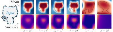
Inspired by the choice made by Dai and Nießner 2022, which we validate experimentally (see Figure 9), we fix .

4.2. Data generation
To evaluate , we first choose to be a loose box around the input point cloud and uniformly sample . Then, as described by Sellán and Jacobson 2022, we compute the matrices
| (19) |
as well as the lumped sample covariance matrix
| (20) |
We employ the same approximated Gaussian kernel suggested by the authors and make use of its compact support to efficiently evaluate the above matrices with a KD tree. Using these matrices, we compute the Gaussian Process posterior mean
| (21) |
where concatenates , and the covariance
| (22) |
The row entries in then correspond to , while each scalar entry in determines the matrix through . As we validate experimentally in Figure 8, sampling uniformly during training is necessary to maintain the theoretical guarantees in Eqs. 14 and 15. More elaborate strategies beyond this work’s scope (e.g., Metropolis-Hastings integration) that would result in weights being added in Eqs. 14 and 15 may yield performance improvements.
4.3. Architecture & Training
We model and using two five-layered MLPs (see Figure 11) with 512 internal hidden units and sine activation functions [Sitzmann et al. 2020]. Our covariance network also includes a SoftPlus layer to enforce positivity, followed by an averaging (see Figure 2). Combined with Schwarz’s theorem, this forces in Eq. (15) to be symmetric by construction. We experimented with residual connection layers as suggested by Yu et al. 2018, but found no significant performance improvement.
At each epoch, we generate 100,000 covariance and 100,000 mean Poisson samples together with an equal number of screening samples selected from the point cloud (with repetition if necessary) as detailed in Section 4.2. This sampling results in four datasets (covariance, mean, covariance screening and mean screening). We cycle through all four with repetition until they are all exhausted with a 512 batch size, evaluating our losses and backpropagating through them to compute the gradient of with respect to . We then use the Adam [Kingma and Ba 2014] optimizer with learning rate and weight decay . We repeat this process for a number of epochs between 50 and 200 (see Figure 10).
Implementation details
We implement our algorithm in Python, using PyTorch to build and train our model and Gpytoolbox [Sellán et al. 2023] for common geometry processing subroutines. In our 3.0Ghz 18-core Linux machine with a 48 GB NVIDIA RTX A6000 graphics card and 528 GB RAM, our unoptimized implementation lasts around 30 seconds to train each epoch, the main bottleneck being the backpropagation through the operator in Eq. (11). For Figures 3 and 4, we implemented the algorithm by Dai and Nießner 2022 following their instructions in the absence of author-provided code. We rendered our 3D results using Blender.
5. Results & Applications
5.1. 3D Scanning integration
Once a point cloud has been captured, our method can be used to compute all kinds of statistical queries useful to the reconstruction (Figure 7) in the same way as described by Sellán and Jacobson 2022. However, our novel neural perspective goes one qualitative step further and allows for a full integration into the scanning process, providing feedback over where to scan next and efficiently updating a given reconstruction upon capturing more data.

5.1.1. Ray casting
Given a captured scan and a proposed sensor position and direction , a crucial question is where a ray travelling from the sensor would intersect the surface. In traditional volumetric rendering terms, this amounts to computing the opacity along the ray, or the likelihood that a ray emanating from the sensor reaches a given distance without terminating.
Sellán and Jacobson 2022 suggest computing the marginal probabilities along the ray
| (23) |
and interpreting these as densities
| (24) |
that they propose integrating to compute the opacity
| (25) |
However, we note that this expression for the opacity is usually employed in the context of gases, for which the effects of inter-particle interactions are negligible and one can assume that the likelihood of encountering a gas particle at time is independent of encountering one at time , giving validity to the integral in Eq. (25). This independence assumption does not hold for the case of uncertain solids, as evidenced by Figure 13: while the marginal likelihood is for all between and , there is no configuration of the shape for which a ray terminates at . Statistically, this is because the point at time is fully correlated with the point at time . While Figure 13 is an extreme example, this difference appears in general reconstruction examples (see Figure 14)
Accounting for these correlations is simple. Instead of Eq. (25), one can compute the opacity as the joint probability that was positive at every point in the ray prior to :
| (26) |
We uniformly discretize the interval such that it amounts to querying a cumulative multivariate Gaussian. Fortunately, as shown by Marmin et al. 2015, this expression can be differentiated with respect to the entries in the covariance matrix with the aid of Plackett’s formula [Berman 1987]. We use the PyTorch implementation of this formula by Marmin 2023 for this task.

5.1.2. Next view planning
As seen above, the time travelled by a ray from a given camera position before colliding with the surface can be interpreted as a random variable, whose cumulative distribution function is the opacity in Eq. (26). Crucially, by Foubini’s theorem, this means one can compute the expected collision time as
| (27) |
leading to the expected collision point
| (28) |
The optimal sensor position will be one that generates a new point cloud point in an area of high variance. Therefore, it makes sense to define the score of a camera as
| (29) |
While Sellán and Jacobson 2022 propose a camera scoring criteria, our novel neural perspective allows us to backpropagate through , meaning that we can compute the gradient of the score with respect to camera parameters , and find an optimal camera position with gradient descent. We show the potential of this contribution in Figure 6, inspired by Fig. 26 by Sellán and Jacobson 2022.
This gradient-based next view angle optimization will often converge to suboptimal local minima. Indeed, as we show in Figure 12, it is better combined with a global search by sampling several initial sensor positions, backpropagating to find an optimum near them, and then choosing the converged camera with the best global score. In Figure 15, we quantify the quality of our subsequent chosen views of a mechanical object by showing they improve on randomly sampled ones. Only in this simplified setup in which views are sampled from a sphere around the object and the directions are constrained to aim to the same spatial point, we are able to compare also to other heuristics like furthest-point sampling, which we show our more generally applicable method matches or outperforms.


5.1.3. Fine-tuning
Once a new sensor position is chosen and a new scan is taken, points are added to the cloud. Traditional algorithms like PSR would then require investing in an updated discretization and entirely new Poisson solve to obtain an updated reconstruction.
Fortunately, our neural perspective allows us to take advantage of an earlier reconstruction to update it more efficiently. Indeed, as shown in Figure 16, we may consider our model’s training on the initial point cloud as a pretraining of our model, which is fine-tuned for only a few epochs every time new points are captured.
Our model can thus be integrated in an end-to-end scanning pipeline, as once an updated mean and variance is obtained, the best next view angle optimization can start again (see Figure 1). Our algorithm can even provide a stopping criterion, in the form of the integrated uncertainty proposed by Sellán and Jacobson 2022.
5.2. Generalization
Another major advantage of our neural formalism over a traditional one is the possibility to train our network on many given reconstructions and trust it to generalize to similar-yet-unseen data. This can circumvent expensive optimizations in cases where one has access to a large training set of point clouds and must quickly make inference on a newly observed set of points.
We show a prototypical example of what such a process could look like in Figure 17, where a training set of point clouds is captured by scanning a shape from several different angles. Our model is then expanded to accept a latent encoding , the values of which are trained simultaneously with the model parameters in the “autodecoder” style proposed by Park et al. 2019. When a new scan of the object is captured, test-time optimization (with the model parameters frozen) produces an optimal latent encoding for the new point cloud. This reconstruction can be used as-is or fine-tuned for a very limited number of epochs for a final reconstruction.
We believe this generalization capability can prove useful in industrial applications, where one may be able to produce a number of partial training scans of an object. Then, objects on an assembly line can be quickly scanned and projected into the learned latent space of partial scans. As we show in Figure 18, our model’s statistical formalism can then be used (in the form of the point cloud’s average log likelihood) to identify foreign objects or defective pieces.
One can also use our model to generalize over a space of different-yet-similar shapes, as we show in Figure 19, where a latent space of scans is learned over 20 diverse human scans generated using STAR [Osman et al. 2020]. Upon capturing a new scan, test-time latent code optimization can efficiently provide a novel reconstruction.


6. Limitations & Conclusion
As we have shown, a key advantage of our neural formulation is the possibility to iteratively fine-tune reconstructions upon capturing more data. To fully take advantage of our method’s efficiency, one may need to optimize its runtime, which we did not do beyond asymptotics. We believe the clearest avenues for speedups are exploring non-uniform distributions for data generation and task-specific weight initializations.
We introduce a method for formalizing reconstruction uncertainty using a neural network. However, it should be noted that this uncertainty is encoded by the Gaussian Process used to generate data, while the network is merely solving a PDE. A promising avenue for future work is circumventing the GP altogether, using Machine Learning uncertainty quantification techniques to obtain a posterior distribution directly from the input point cloud. While this may mean deviating from Poisson Surface Reconstruction, it could present a major improvement in accuracy (removing the need for covariance matrix lumping) and applicability (allowing for sensor-specific non-Gaussian noise patterns).
All our generalization results (Figures 17, 18 and 19) use identical (virtual) scanning devices, and every input point cloud is re-scaled to the unit cube; as such, we do not expect our results to generalize beyond these choices. Future work could mitigate this; for example, by learning a latent space of device parameters and positions as suggested by Martin-Brualla et al. 2021 in the context of NeRF.
While uncertainty quantification has become a common consideration in neighboring fields like Computer Vision and Robotics [Kendall and Gal 2017], it remains rare for Computer Graphics works to expose their algorithmic uncertainties. It is our hope that as our tool set grows and our field’s application realm diversifies, our work can serve as a first step in the right direction.


Acknowledgements.
This project is funded in part by NSERC Discovery (RGPIN2017-05235, RGPAS-2017-507938), New Frontiers of Research Fund (NFRFE-201), the Ontario Early Research Award program, the Canada Research Chairs Program, a Sloan Research Fellowship and the DSI Catalyst Grant program. The first author is funded in part by an NSERC Vanier Scholarship. We thank Kirill Serkh, Kiriakos Kutulakos, David Lindell, Eitan Grinspun, David I.W. Levin, Oded Stein, Andrea Tagliasacchi, Otman Benchekroun, Lily Goli and Claas A. Voelcker for insightful conversations that inspired us in this work; Hsueh-Ti Derek Liu for his help rendering our results; as well as Rafael Rodrigues (Fig. 6, CC BY-NC-SA 4.0) and ShaggyDude (Fig. 13, CC BY 4.0) for releasing their 3D models for academic use. We would also like to thank Xuan Dam, John Hancock and all the University of Toronto Department of Computer Science research, administrative and maintenance staff.References
- [1]
- Alexa et al. [2003] Marc Alexa, Johannes Behr, Daniel Cohen-Or, Shachar Fleishman, David Levin, and Claudio T. Silva. 2003. Computing and rendering point set surfaces. IEEE TVCG 9, 1 (2003), 3–15.
- Berger et al. [2017] Matthew Berger, Andrea Tagliasacchi, Lee M Seversky, Pierre Alliez, Gael Guennebaud, Joshua A Levine, Andrei Sharf, and Claudio T Silva. 2017. A survey of surface reconstruction from point clouds. In Comput. Graph. Forum, Vol. 36. Wiley Online Library, 301–329.
- Berman [1987] Simeon M Berman. 1987. An extension of Plackett’s differential equation for the multivariate normal density. SIAM Journal on Algebraic Discrete Methods 8, 2 (1987), 196–197.
- Bircher et al. [2016] Andreas Bircher, Mina Kamel, Kostas Alexis, Helen Oleynikova, and Roland Siegwart. 2016. Receding horizon" next-best-view" planner for 3d exploration. In 2016 IEEE international conference on robotics and automation (ICRA). IEEE, 1462–1468.
- Carr et al. [2001] Jonathan C Carr, Richard K Beatson, Jon B Cherrie, Tim J Mitchell, W Richard Fright, Bruce C McCallum, and Tim R Evans. 2001. Reconstruction and representation of 3D objects with radial basis functions. In Proceedings of the 28th annual conference on Computer graphics and interactive techniques. 67–76.
- Chen et al. [2011] Shengyong Chen, Youfu Li, and Ngai Ming Kwok. 2011. Active vision in robotic systems: A survey of recent developments. The International Journal of Robotics Research 30, 11 (2011), 1343–1377.
- Connolly [1985] Cl Connolly. 1985. The determination of next best views. In Proceedings. 1985 IEEE international conference on robotics and automation, Vol. 2. IEEE, 432–435.
- Cuomo et al. [2022] Salvatore Cuomo, Vincenzo Schiano Di Cola, Fabio Giampaolo, Gianluigi Rozza, Maziar Raissi, and Francesco Piccialli. 2022. Scientific machine learning through physics–informed neural networks: where we are and what’s next. Journal of Scientific Computing 92, 3 (2022), 88.
- Dai and Nießner [2022] Angela Dai and Matthias Nießner. 2022. Neural Poisson: Indicator Functions for Neural Fields. arXiv preprint arXiv:2211.14249 (2022).
- Daudelin and Campbell [2017] Jonathan Daudelin and Mark Campbell. 2017. An adaptable, probabilistic, next-best view algorithm for reconstruction of unknown 3-d objects. IEEE Robotics and Automation Letters 2, 3 (2017), 1540–1547.
- Groueix et al. [2018] Thibault Groueix, Matthew Fisher, Vladimir G Kim, Bryan C Russell, and Mathieu Aubry. 2018. A papier-mâché approach to learning 3d surface generation. In Proc. CVPR. 216–224.
- Hoppe et al. [1992] Hugues Hoppe, Tony DeRose, Tom Duchamp, John McDonald, and Werner Stuetzle. 1992. Surface reconstruction from unorganized points. In Proceedings of the 19th annual conference on computer graphics and interactive techniques. 71–78.
- Isler et al. [2016] Stefan Isler, Reza Sabzevari, Jeffrey Delmerico, and Davide Scaramuzza. 2016. An information gain formulation for active volumetric 3D reconstruction. In 2016 IEEE International Conference on Robotics and Automation (ICRA). IEEE, 3477–3484.
- Jin et al. [2023] Liren Jin, Xieyuanli Chen, Julius Rückin, and Marija Popović. 2023. NeU-NBV: Next Best View Planning Using Uncertainty Estimation in Image-Based Neural Rendering. arXiv preprint arXiv:2303.01284 (2023).
- Kazhdan et al. [2006] Michael Kazhdan, Matthew Bolitho, and Hugues Hoppe. 2006. Poisson surface reconstruction. In Proc. SGP, Vol. 7. 0.
- Kazhdan and Hoppe [2013] Michael Kazhdan and Hugues Hoppe. 2013. Screened poisson surface reconstruction. ACM Trans. Graph. 32, 3 (2013), 1–13.
- Kendall and Gal [2017] Alex Kendall and Yarin Gal. 2017. What uncertainties do we need in bayesian deep learning for computer vision? Proc. NeurIPS 30 (2017).
- Kingma and Ba [2014] Diederik P Kingma and Jimmy Ba. 2014. Adam: A method for stochastic optimization. arXiv preprint arXiv:1412.6980 (2014).
- Kong et al. [2023] Xin Kong, Shikun Liu, Marwan Taher, and Andrew J Davison. 2023. vMAP: Vectorised Object Mapping for Neural Field SLAM. arXiv preprint arXiv:2302.01838 (2023).
- König and Gumhold [2009] Sören König and Stefan Gumhold. 2009. Consistent Propagation of Normal Orientations in Point Clouds.. In VMV. 83–92.
- Lauri et al. [2020] Mikko Lauri, Joni Pajarinen, Jan Peters, and Simone Frintrop. 2020. Multi-Sensor Next-Best-View Planning as Matroid-Constrained Submodular Maximization. IEEE Robotics and Automation Letters 5, 4 (Oct. 2020), 5323–5330. https://doi.org/10.1109/LRA.2020.3007445 arXiv:2007.02084
- Levin [2004] David Levin. 2004. Mesh-independent surface interpolation. In Geometric modeling for scientific visualization. Springer, 37–49.
- Marmin [2023] Sébastien Marmin. 2023. Torch-MvNorm. https://github.com/SebastienMarmin/torch-mvnorm.
- Marmin et al. [2015] Sébastien Marmin, Clément Chevalier, and David Ginsbourger. 2015. Differentiating the multipoint expected improvement for optimal batch design. In International Workshop on Machine Learning, Optimization and Big Data. Springer, 37–48.
- Martin-Brualla et al. [2021] Ricardo Martin-Brualla, Noha Radwan, Mehdi SM Sajjadi, Jonathan T Barron, Alexey Dosovitskiy, and Daniel Duckworth. 2021. Nerf in the wild: Neural radiance fields for unconstrained photo collections. In Proceedings of the IEEE/CVF Conference on Computer Vision and Pattern Recognition. 7210–7219.
- Metzer et al. [2021] Gal Metzer, Rana Hanocka, Denis Zorin, Raja Giryes, Daniele Panozzo, and Daniel Cohen-Or. 2021. Orienting point clouds with dipole propagation. ACM Trans. Graph. 40, 4 (2021), 1–14.
- Mildenhall et al. [2021] Ben Mildenhall, Pratul P Srinivasan, Matthew Tancik, Jonathan T Barron, Ravi Ramamoorthi, and Ren Ng. 2021. Nerf: Representing scenes as neural radiance fields for view synthesis. Commun. ACM 65, 1 (2021), 99–106.
- Ohtake et al. [2005] Yutaka Ohtake, Alexander Belyaev, Marc Alexa, Greg Turk, and Hans-Peter Seidel. 2005. Multi-level partition of unity implicits. In Acm Siggraph 2005 Courses. 173–es.
- Osman et al. [2020] Ahmed AA Osman, Timo Bolkart, and Michael J Black. 2020. Star: Sparse trained articulated human body regressor. In Proc. ECCV. Springer, 598–613.
- Özyeşil et al. [2017] Onur Özyeşil, Vladislav Voroninski, Ronen Basri, and Amit Singer. 2017. A survey of structure from motion*. Acta Numerica 26 (2017), 305–364.
- Park et al. [2019] Jeong Joon Park, Peter Florence, Julian Straub, Richard Newcombe, and Steven Lovegrove. 2019. Deepsdf: Learning continuous signed distance functions for shape representation. In Proc. CVPR. 165–174.
- Pauly et al. [2004] Mark Pauly, Niloy J Mitra, and Leonidas J Guibas. 2004. Uncertainty and variability in point cloud surface data.. In PBG. 77–84.
- Pauly et al. [2008] Mark Pauly, Niloy J Mitra, Johannes Wallner, Helmut Pottmann, and Leonidas J Guibas. 2008. Discovering structural regularity in 3D geometry. ACM Trans. Graph. (2008), 1–11.
- Raj et al. [2020] Thinal Raj, Fazida Hanim Hashim, Aqilah Baseri Huddin, Mohd Faisal Ibrahim, and Aini Hussain. 2020. A survey on LiDAR scanning mechanisms. Electronics 9, 5 (2020), 741.
- Remil et al. [2017] Oussama Remil, Qian Xie, Xingyu Xie, Kai Xu, and Jun Wang. 2017. Surface reconstruction with data-driven exemplar priors. 88 (2017), 31–41.
- Schertler et al. [2017] Nico Schertler, Bogdan Savchynskyy, and Stefan Gumhold. 2017. Towards globally optimal normal orientations for large point clouds. In Comput. Graph. Forum, Vol. 36. Wiley Online Library, 197–208.
- Schnabel et al. [2009] Ruwen Schnabel, Patrick Degener, and Reinhard Klein. 2009. Completion and reconstruction with primitive shapes. In Comput. Graph. Forum, Vol. 28. Wiley Online Library, 503–512.
- Scott et al. [2003] William R Scott, Gerhard Roth, and Jean-François Rivest. 2003. View planning for automated three-dimensional object reconstruction and inspection. ACM Computing Surveys (CSUR) 35, 1 (2003), 64–96.
- Sellán and Jacobson [2022] Silvia Sellán and Alec Jacobson. 2022. Stochastic Poisson Surface Reconstruction. ACM Trans. Graph. 41, 6 (2022), 1–12.
- Sellán et al. [2023] Silvia Sellán, Oded Stein, et al. 2023. gptyoolbox: A Python Geometry Processing Toolbox. https://gpytoolbox.org/.
- Sharf et al. [2007] Andrei Sharf, Thomas Lewiner, Gil Shklarski, Sivan Toledo, and Daniel Cohen-Or. 2007. Interactive topology-aware surface reconstruction. ACM Trans. Graph. 26, 3 (2007), 43–es.
- Sitzmann et al. [2020] Vincent Sitzmann, Julien N.P. Martel, Alexander W. Bergman, David B. Lindell, and Gordon Wetzstein. 2020. Implicit Neural Representations with Periodic Activation Functions. In Proc. NeurIPS.
- Smith et al. [2022] Edward J Smith, Michal Drozdzal, Derek Nowrouzezahrai, David Meger, and Adriana Romero-Soriano. 2022. Uncertainty-Driven Active Vision for Implicit Scene Reconstruction. arXiv preprint arXiv:2210.00978 (2022).
- Sucar et al. [2021] Edgar Sucar, Shikun Liu, Joseph Ortiz, and Andrew J Davison. 2021. iMAP: Implicit mapping and positioning in real-time. In Proc. ICCV. 6229–6238.
- Vasquez-Gomez et al. [2014] J Irving Vasquez-Gomez, L Enrique Sucar, Rafael Murrieta-Cid, and Efrain Lopez-Damian. 2014. Volumetric next-best-view planning for 3D object reconstruction with positioning error. International Journal of Advanced Robotic Systems 11, 10 (2014), 159.
- Williams et al. [2019] Francis Williams, Teseo Schneider, Claudio Silva, Denis Zorin, Joan Bruna, and Daniele Panozzo. 2019. Deep geometric prior for surface reconstruction. In Proc. CVPR. 10130–10139.
- Xu et al. [2015] Kai Xu, Hui Huang, Yifei Shi, Hao Li, Pinxin Long, Jianong Caichen, Wei Sun, and Baoquan Chen. 2015. Autoscanning for coupled scene reconstruction and proactive object analysis. ACM Trans. Graph. 34, 6 (2015), 1–14.
- Yamauchi [1997] Brian Yamauchi. 1997. A frontier-based approach for autonomous exploration. In Proceedings 1997 IEEE International Symposium on Computational Intelligence in Robotics and Automation CIRA’97.’Towards New Computational Principles for Robotics and Automation’. IEEE, 146–151.
- Yu et al. [2018] Bing Yu et al. 2018. The deep Ritz method: a deep learning-based numerical algorithm for solving variational problems. Communications in Mathematics and Statistics 6, 1 (2018), 1–12.
- Zhang et al. [2021] Han Zhang, Yucong Yao, Ke Xie, Chi-Wing Fu, Hao Zhang, and Hui Huang. 2021. Continuous aerial path planning for 3D urban scene reconstruction. ACM Trans. Graph. 40, 6 (2021), 225–1.
- Zhou et al. [2020] Xiaohui Zhou, Ke Xie, Kai Huang, Yilin Liu, Yang Zhou, Minglun Gong, and Hui Huang. 2020. Offsite aerial path planning for efficient urban scene reconstruction. ACM Trans. Graph. 39, 6 (2020), 1–16.
