A Finite-Volume Scheme for
Fractional Diffusion on Bounded Domains

Rafael Bailo Affiliation: Mathematical Institute, University of Oxford José A. Carrillo Affiliation: Mathematical Institute, University of Oxford
Stefano Fronzoni Affiliation: Mathematical Institute, University of Oxford David Gómez-Castro Affiliation: OX2 6GG Oxford, United Kingdom Affiliation: bailo@maths.ox.ac.uk, carrillo@maths.ox.ac.uk, fronzoni@maths.ox.ac.uk Affiliation: Affiliation: Ciudad Universitaria de Cantoblanco, 28049 Madrid, Spain Affiliation: david.gomezcastro@uam.es Affiliation: Mathematical Institute, University of Oxford Affiliation: Departamento de Matemáticas, Universidad Autónoma de Madrid

Abstract

We propose a new fractional Laplacian for bounded domains, expressed as a conservation law and thus particularly suited to finite-volume schemes. Our approach permits the direct prescription of no-flux boundary conditions. We first show the well-posedness theory for the fractional heat equation. We also develop a numerical scheme, which correctly captures the action of the fractional Laplacian and its anomalous diffusion effect. We benchmark numerical solutions for the Lévy-Fokker-Planck equation against known analytical solutions. We conclude by numerically exploring properties of these equations with respect to their stationary states and long-time asymptotics.

AMS Subject Classification — 35R11; 65N08.

Keywords — Fractional Laplacian; Levy-Fokker-Planck equation; finite-volume schemes.

1 Introduction

The aim of this work is the design of a finite-volume numerical scheme to approximate the solution of the non-local diffusion problem given by the fractional heat equation and the related Lévy-Fokker-Planck equation. The fractional heat equation is defined in ${\mathbb{R}^{d}}$ as

\frac{\partial\rho}{\partial t}=-(-\Delta)^{\frac{\alpha}{2}}\rho

(1.1)

for $0<\alpha\leq 2$ . The so-called fractional Laplacian, $(-\Delta)^{\frac{\alpha}{2}}\rho$ , can be formally defined by its Fourier symbol $|\xi|^{\alpha}\hat{\rho}$ , although it admits up to ten equivalent definitions (see [28]). There is a suitable self-similar change of variables that leads to $\frac{\partial\rho}{\partial t}=\nabla\cdot(x\rho)-(-\Delta)^{\frac{\alpha}{2}}\rho$ , a particular case of Lévy-Fokker-Planck equation given by

\frac{\partial\rho}{\partial t}=\nabla\cdot(\beta x\rho)-(-\Delta)^{\frac{\alpha}{2}}\rho

(1.2)

for $0<\alpha\leq 2$ and $\beta\geq 0$ . Notice that this equation generalises the usual Fokker-Planck equation $\frac{\partial\rho}{\partial t}=\nabla\cdot(\beta x\rho)+\Delta\rho$ by replacing the Laplacian with a fractional operator, see [8, 24].

Fractional diffusion (in particular, the fractional Laplacian) has been shown to be the mean field limit of Lévy walks under certain scalings [40]. This kind of stochastic process consists in the random movement of particles in space, subject to a probability that allows long jumps with a polynomial tail. Such random walks are long range stochastic processes and they are generally considered more realistic in the modelling of certain biological phenomena [22, 32, 11, 21, 29].

The inverse Fourier transform of the symbol $|\xi|^{\alpha}\hat{\rho}$ yields, after some work, the Riesz or singular integral definition of the fractional Laplacian:

\displaystyle(-\Delta)^{\frac{\alpha}{2}}\rho(x)\coloneqq\mathcal{C}(d,\alpha)\;\textrm{p.v.}\int_{\mathbb{R}^{d}}\frac{\rho(x)-\rho(y)}{\left|x-y\right|^{d+\alpha}}\mathop{}\!\mathrm{d}y,

(1.3)

where the integral is understood in the Cauchy principal value sense in order to overcome the singularity. The constant $\mathcal{C}(d,\alpha)$ , a term which arises in the computation of the inverse transform of $|\xi|^{\alpha}$ , is given by

\displaystyle\mathcal{C}(d,\alpha)=\frac{2^{\alpha}\Gamma\left(\frac{d+\alpha}{2}\right)}{\pi^{\frac{d}{2}}\left|\Gamma\left(-\frac{\alpha}{2}\right)\right|}.

(1.4)

Using the Riesz potential, Eq. 1.2 can be formally written in divergence form as

\frac{\partial\rho}{\partial t}+\nabla\cdot F=0,\quad\text{where }F=-\beta x\rho+\nabla\left[(-\Delta)^{\frac{\alpha}{2}-1}\rho\right].

(1.5)

The advantage of this form is that the fractional operator now appears with a negative exponent. In this case, the inverse Fourier transform of the symbol $|\xi|^{-\alpha}\hat{\rho}$ yields (see [38, Chapter 5])

\displaystyle(-\Delta)^{-\frac{\alpha}{2}}\rho(x)=\mathcal{C}(d,-\alpha)\int_{\mathbb{R}^{d}}\frac{\rho(y)}{\left|x-y\right|^{d-\alpha}}\mathop{}\!\mathrm{d}y

(1.6)

whenever $0<\alpha<d$ . This form for the inverse operator bypasses the singularity altogether. Equation 1.5 can therefore be rewritten as

\frac{\partial\rho}{\partial t}+\nabla\cdot F=0,\quad\text{where }F=-\beta x\rho+\mathcal{C}(d,\alpha-2)\nabla\int_{\mathbb{R}^{d}}\frac{\rho(y)}{\left|x-y\right|^{d+\alpha-2}}\mathop{}\!\mathrm{d}y

(1.7)

whenever $\alpha>2-d$ . Therefore, in dimension one this formulation is only valid for $1<\alpha\leq 2$ ; in higher dimensions, for $0<\alpha\leq 2$ . This new form of the equation has two advantages: the first, that the fractional operator is no longer singular; and the second, that an equation in divergence form lends itself to be discretised in the finite-volume fashion. Finite volume schemes have been used with success to produce structure preserving schemes for equations in divergence form of gradient flow type and related systems, see [15, 5, 6, 16]. This is a departure from the numerical methods for fractional diffusions that have been developed in the past, where the literature has been focused on finite-element and finite-difference methods [20, 25, 35, 3, 18, 4, 10, 33]. We also highlight several spectral methods [34, 37, 17, 41] which deal exclusively with problems on unbounded domains.

For the sake of computation, we would like to pose Eq. 1.2 on an open bounded domain $\Omega\subset{\mathbb{R}^{d}}$ . There are several non-equivalent definitions of fractional-type Laplacians on bounded domains that can be obtained as suitable restrictions of the definitions in ${\mathbb{R}^{d}}$ (see [1, Section 1.2] and the references therein). In this work, we construct a new fractional Laplacian by restricting Eq. 1.7 to the domain $\Omega$ , prescribing zero-flux conditions for the divergence, and extending the density as $\rho\equiv 0$ on ${\mathbb{R}^{d}}\setminus\Omega$ in order to ensure that the non-local operator is well-defined. Thus, our interpretation of the Lévy-Fokker-Planck equation on a bounded domain is

\left\{\begin{aligned} &\frac{\partial\rho}{\partial t}+\nabla\cdot F=0,\\ &F=-\beta x\rho+\mathcal{C}(d,\alpha)\nabla\int_{\Omega}\frac{\rho(y)}{\left|x-y\right|^{d+\alpha-2}}\mathop{}\!\mathrm{d}y,\\ &F\cdot n_{\partial\Omega}=0.\end{aligned}\right.

(1.8)

In the absence of a drift term (when $\beta=0$ ), we also obtain an interpretation of the fractional heat equation on a bounded domain. Notice, however, that the steady states of this problem will satisfy

\int_{\Omega}\frac{\rho_{\infty}(y)}{\left|x-y\right|^{d+\alpha-2}}\mathop{}\!\mathrm{d}y=C,

(1.9)

which causes $\rho_{\infty}$ to be singular on the boundary. However, for $\beta>0$ , our numerical results on suitably scaled quadrangular domains show that the numerical steady state is very similar to the self-similar profile of the ${\mathbb{R}^{d}}$ case (see Sections 4.2.1 and 4.1.3).

The rest of this work is organised as follows: in Section 2 we study the well-posedness of Eq. 1.8, distinguishing the cases $\beta=0$ and $\beta>0$ ; in Section 3 we introduce a finite-volume numerical scheme for Eq. 1.8 in one dimension, and then generalise it to higher dimensions via dimensional splitting; we conclude in Section 4 by validating our schemes against known analytical results.

2 A new fractional Laplacian in bounded domains

The aim of this section is to establish a well-posedness theory for the new fractional operator on a bounded domain introduced above. We first define the Riesz kernel and the extension operator

\mathcal{I}_{\gamma}[u](x)=\mathcal{C}(d,-\gamma)\int_{\mathbb{R}^{d}}\frac{u(y)}{|x-y|^{d-\gamma}}dy,\qquad\qquad\mathcal{E}[u](x)=\begin{cases}u(x)&\text{if }x\in\Omega,\\ 0&\text{otherwise},\end{cases}

(2.1)

where we assume that $0<\gamma<d$ for the operator to be well defined. The operator $\mathcal{I}_{\gamma}:L^{p}(\mathbb{R}^{d})\to L^{q}(\mathbb{R}^{d})$ has been widely studied. Note that the flux in Eq. 1.8 reduces, whenever $\beta=0$ , to

F=\nabla\Big(\mathcal{I}_{2(1-\frac{\alpha}{2})}\mathcal{E}u\Big).

(2.2)

Thus, besides $\alpha\in(0,2)$ , we require $0<2(1-\frac{\alpha}{2})<d$ for well-posedness, i.e. $\alpha>2-d$ . This is only restrictive in dimension $d=1$ .

Let $\mathcal{B}=\mathcal{I}_{2(1-\frac{\alpha}{2})}\mathcal{E}$ . If $\Omega={\mathbb{R}^{d}}$ , then $\mathcal{B}=(-\Delta)^{-(1-\frac{\alpha}{2})}$ , an inverse fractional Laplacian. Our new diffusion operator is therefore $\mathcal{A}=-\Delta\mathcal{B}u$ , and we denote its domain by $D(\mathcal{A})$ . Equation 1.8 can be now written in the $\beta=0$ case as

\begin{cases}\frac{\partial u}{\partial t}=\Delta\mathcal{B}u&\text{in }(0,\infty)\times\Omega,\\ \frac{\partial(\mathcal{B}u)}{\partial n}=0&\text{on }(0,\infty)\times\Omega.\end{cases}

(2.3)

Theorem 2.1.

There exists a unique semigroup $\mathcal{S}(t):L^{2}(\Omega)\to L^{2}(\Omega)$ of solutions of (2.3). In fact, if $\mathcal{B}u_{0}\in H^{2}(\Omega)$ then $\mathcal{B}u(t)\in H^{2}(\Omega)$ for all times and the equation is satisfied in the operator sense.

Proof.

We will first justify the well-posedness of this problem using the Hille-Yosida theorem applied to the operator $\mathcal{A}$ with the Neumann condition in $L^{2}(\Omega)$ (see [12, Theorem 7.4]).

Let us construct $D(\mathcal{A})$ . We begin by remarking that $\mathcal{B}:L^{2}(\Omega)\to L^{2}(\Omega)$ is self-adjoint, since

\int_{\Omega}v(x)\mathcal{B}u(x)\mathop{}\!\mathrm{d}x=\int_{\Omega}\int_{\Omega}\frac{u(y)v(x)}{|x-y|^{d-2(1-\frac{\alpha}{2})}}\mathop{}\!\mathrm{d}x\mathop{}\!\mathrm{d}y=\int_{\Omega}u(y)\mathcal{B}v(y)\mathop{}\!\mathrm{d}y.

(2.4)

Since $\mathcal{I}_{\alpha}$ is a compact operator on $L^{2}_{c}({\mathbb{R}^{d}})$ , so is $\mathcal{B}$ in $L^{2}(\Omega)$ . Thus, by the spectral theorem, there exists a basis of $L^{2}(\Omega)$ of orthonormal eigenfunctions $\varphi_{i}$ of $\mathcal{B}$ with eigenvalues $\lambda_{i}\to 0$ , and, defining $u_{i}=\int_{\Omega}u\varphi_{i}\mathop{}\!\mathrm{d}x$ , it holds

u(x)=\sum_{i=1}^{\infty}u_{i}\varphi_{i}(x),\qquad\text{and}\qquad\mathcal{B}u(x)=\sum_{i=1}^{\infty}\lambda_{i}u_{i}\varphi_{i}(x).

(2.5)

Furthermore, with this construction $\|u\|_{L^{2}}=\sum_{i}|u_{i}|^{2}$ .

Let us show that $\lambda_{i}\geq 0$ . Defining $U\coloneqq\mathcal{B}u$ , notice that $(-\Delta)^{1-\frac{\alpha}{2}}U=\mathcal{E}(u)$ in ${\mathbb{R}^{d}}$ . Therefore, for $u\in C_{c}^{\infty}(\Omega)$ , we have

\int_{\Omega}u\mathcal{B}u=\int_{\Omega}U(-\Delta)^{1-\frac{\alpha}{2}}U=\int_{\mathbb{R}^{d}}U(-\Delta)^{1-\frac{\alpha}{2}}U=\int_{\mathbb{R}^{d}}\left|(-\Delta)^{\frac{1-\frac{\alpha}{2}}{2}}U\right|^{2}\geq 0.

(2.6)

Hence $\lambda_{i}\geq 0$ .

We now show that $\lambda_{i}>0$ for all $i$ . Suppose, to the contrary, that $\lambda_{i}=0$ for some $i$ . We therefore have that $U\coloneqq\mathcal{B}\varphi_{i}=0$ . But then, a.e. in $\Omega$ we have that $\varphi_{i}=\mathcal{E}(\varphi_{i})=(-\Delta)^{1-\frac{\alpha}{2}}U=0$ , a contradiction.

Therefore, we can formally define the operator $\mathcal{B}^{-1}$ through the series $\mathcal{B}^{-1}u(x)=\sum_{i}\lambda_{i}^{-1}u_{i}\varphi_{i}(x)$ . We define

D(\mathcal{A})=\left\{u=\mathcal{B}^{-1}v:v\in H^{2}(\Omega),\nabla v\cdot n=0\text{ on }\partial\Omega\text{, and }\sum_{i}\lambda_{i}^{-2}|v_{i}|^{2}<\infty\right\}.

(2.7)

Notice, by construction, that $D(\mathcal{A})=L^{2}(\Omega)\cap\mathcal{B}^{-1}(H^{2}(\Omega))$ . Since $\lambda_{i}>0$ , this set is not empty. Then $\mathcal{A}:D(\mathcal{A})\subset L^{2}(\Omega)\to L^{2}(\Omega)$ .

Now we check that $\mathcal{A}$ is monotone. Take $u\in D(\mathcal{A})$ . Due the spectral decomposition of $\mathcal{B}$ it admits a square root and inverse square root $\mathcal{B}^{\pm\frac{1}{2}}$ ; take $w=\mathcal{B}^{\frac{1}{2}}u$ . Then, due to the Neumann boundary condition

\int_{\Omega}u(\mathcal{A}u)=\int_{\Omega}\nabla u\cdot\nabla\mathcal{A}u=\int_{\Omega}|\nabla\mathcal{B}^{\frac{1}{2}}w|^{2}\geq 0.

(2.8)

Lastly, we check that $\mathcal{A}$ is maximal monotone. Take $f\in L^{2}(\Omega)$ ; we want to show there exists $u\in D(\mathcal{A})$ such that $u+\mathcal{A}u=f$ . Consider the weak formulation

\int_{\Omega}u\varphi+\int_{\Omega}\nabla\mathcal{B}u\cdot\nabla\varphi=\int_{\Omega}f\varphi,\qquad\forall\varphi\in H^{1}(\Omega).

(2.9)

Letting again $w=\mathcal{B}^{\frac{1}{2}}u$ and $\psi=\mathcal{B}^{-\frac{1}{2}}\varphi$ , we obtain

\int_{\Omega}w\psi+\int_{\Omega}\nabla\mathcal{B}^{\frac{1}{2}}w\cdot\nabla\mathcal{B}^{\frac{1}{2}}\psi=\int_{\Omega}\mathcal{B}^{-\frac{1}{2}}w\mathcal{B}^{\frac{1}{2}}\psi+\int_{\Omega}\nabla\mathcal{B}^{\frac{1}{2}}w\cdot\nabla\mathcal{B}^{\frac{1}{2}}\psi=\int_{\Omega}f\mathcal{B}^{\frac{1}{2}}\psi.

(2.10)

This is a problem of the form $a(w,\psi)=L(\psi)$ where $w,\psi\in V=\mathcal{B}^{-\frac{1}{2}}(H^{1}(\Omega))\cap L^{2}(\Omega)$ , where the bilinear form $a$ is symmetric and continuous in $V$ . Hence, it can be solved using the Lax-Milgram theorem. A posteriori, it is trivial to verify that $u\in D(\mathcal{A})$ .

We now satisfy all the hypotheses of the Hille-Yosida theorem. Thus, if $u_{0}\in D(\mathcal{A})$ , then $\mathcal{S}(t)u_{0}$ is a solution in the strong sense, i.e. $u\in C([0,\infty),D(A))\cap C^{1}([0,\infty),L^{2}(\Omega))$ and the equation is satisfied. ∎

The problem (1.8) is not purely diffusive when $\beta>0$ , hence the existence does not follow directly from the Hille-Yosida (or Lumer-Phillips) theorems. Unlike in ${\mathbb{R}^{d}}$ , it cannot be deduced from the diffusive problem by a change of variables; that would lead to a domain $\Omega_{t}$ that evolves in time. Thus the theory of well-posedness for (1.8) when $\beta>0$ is an open problem. A sensible approach would be to prove the convergence of our numerical scheme below.

3 Numerical schemes

The thrust of this work is the discretisation of the fractional Laplacian term in Eq. 1.8. First we introduce the scheme in one spatial dimension, in order to highlight the technique used to approximate the fractional term, and then we generalise it to higher dimensions. Our discretisation of the advection term follows previous finite-volume works for generalised Fokker-Planck equations.

3.1 One dimension

In one dimension, we construct a scheme for Eq. 1.8 in the range $1<\alpha<2$ . We consider, without loss of generality, a domain $\Omega=(-R,R)$ , and divide it into $N$ cells $C_{i}=[x_{i-\frac{1}{2}},x_{i+\frac{1}{2}}]$ , for $i=1,\cdots,N$ . Each cell is centred at the points $x_{i}$ , where $x_{i}=-R+(i-1/2)\Delta x$ . For simplicity, we assume a uniform grid with cell size $\Delta x=2RN^{-1}$ .

We denote by $\bar{\rho}_{i}(t)$ the average of the solution $\rho(t,x)$ over the $i$ -th cell:

\bar{\rho}_{i}(t)=\frac{1}{\Delta x}\int_{C_{i}}\rho(t,x)\mathop{}\!\mathrm{d}x.

(3.1)

Then, equation (1.8) can be integrated on each cell $C_{i}$ to yield

\frac{\mathrm{d}\bar{\rho}_{i}(t)}{\mathrm{d}t}+\frac{F\left[\rho(t,x_{i+\frac{1}{2}})\right]-F\left[\rho(t,x_{i-\frac{1}{2}})\right]}{\Delta x}=0,\quad i=1,\cdots,N,

(3.2)

which we approximate as


	$\displaystyle\frac{\mathrm{d}\bar{\rho}_{i}(t)}{\mathrm{d}t}+\frac{F_{i+\frac{1}{2}}(t)-F_{i-\frac{1}{2}}(t)}{\Delta x}=0,\quad i=1,\cdots,N.$		(3.3a)
The flux $F$ is split into an advective part $F^{\textrm{ad}}$ and a diffusive part $F^{\textrm{dif}}$ :

	$\displaystyle F_{i+\frac{1}{2}}(t)=F^{\textrm{ad}}_{i+\frac{1}{2}}(t)+F^{\textrm{dif}}_{i+\frac{1}{2}}(t).$		(3.3b)
The advection flux corresponds to the discretisation of the Fokker-Planck term $\beta\nabla\cdot(\rho x)$ ; here we follow the discretisation of [15, 5]:

	$\displaystyle F^{\textrm{ad}}_{i+\frac{1}{2}}(t)$	$\displaystyle=\bar{\rho}_{i}(t)(v_{i+\frac{1}{2}})^{+}+\bar{\rho}_{i+1}(t)(v_{i+\frac{1}{2}})^{-},$	(3.3c)
where

	$\displaystyle v_{i+\frac{1}{2}}=-\frac{\xi_{i+1}-\xi_{i}}{\Delta x}\text{ and }\xi_{i}=\beta\frac{\|x_{i}\|^{2}}{2},$		(3.3d)
for $(s)^{+}=\max\{0,s\}$ and $(s)^{-}=\min\{0,s\}$ .

To treat the diffusion, the gradient term $\mathcal{C}(1,\alpha-2)\nabla\int_{\mathbb{R}^{d}}\rho(y)\left|x-y\right|^{1-\alpha}\mathop{}\!\mathrm{d}y$ is replaced by the difference

\displaystyle F^{\textrm{dif}}_{i+\frac{1}{2}}(t)=\frac{I(t,x_{i+1})-I(t,x_{i})}{\Delta x}.

(3.3e)

The term $I(t,x_{i})$ is the approximation of the integral $\mathcal{I}_{2-\alpha}[\rho](x_{i})$ , given as a discrete sum by

\displaystyle I(t,x_{i})

\displaystyle=\sum_{k=1}^{N}\bar{\rho}_{k}(t)I_{k}(x_{i}),\quad\textrm{where}\quad I_{k}(x_{i})\coloneqq\mathcal{C}(1,\alpha-2)\int_{C_{k}}\left|x_{i}-y\right|^{1-\alpha}\mathop{}\!\mathrm{d}y.

(3.3f)

To conclude, we impose no-flux boundary conditions:

\displaystyle F_{1-\frac{1}{2}}(t)=F_{N+\frac{1}{2}}(t)\equiv 0.

(3.3g)

Remark 3.1 (Linearity).

Scheme (3.3) is linear. We can rewrite Eq. 3.3a as a system

\frac{\mathrm{d}\boldsymbol{\bar{\rho}}(t)}{\mathrm{d}t}+A\boldsymbol{\bar{\rho}}(t)=0,

(3.4)

for a vector $\boldsymbol{\bar{\rho}}=\begin{pmatrix}\bar{\rho}_{1}&\cdots&\bar{\rho}_{i}&\cdots&\bar{\rho}_{N}\end{pmatrix}^{\top}$ . As with the flux, the constant matrix $A$ can be split into an advective part and a diffusive part, $A=A^{\textrm{ad}}+A^{\textrm{dif}}$ . The advection matrix is simply

\displaystyle A^{\textrm{ad}}

\displaystyle=\frac{\beta}{\Delta x}\begin{pmatrix}(v_{1+\frac{1}{2}})^{+}&(v_{1+\frac{1}{2}})^{-}\\ \ddots&\ddots&\ddots\\ &-(v_{i-\frac{1}{2}})^{+}&-(v_{i-\frac{1}{2}})^{-}+(v_{i+\frac{1}{2}})^{+}&(v_{i+\frac{1}{2}})^{-}\\ &&\ddots&\ddots&\ddots\\ &&&-(v_{N-\frac{1}{2}})^{+}&-(v_{N-\frac{1}{2}})^{-}\end{pmatrix}.

(3.5)

The diffusion matrix can be written as the product of a discrete Laplacian and a dense matrix, $A^{\textrm{dif}}=LD$ , where

\displaystyle L

\displaystyle=-\frac{1}{\Delta x^{2}}\begin{pmatrix}-1&1\\ 1&-2&1\\ &\ddots&\ddots&\ddots\\ &&1&-2&1\\ &&&1&-1\end{pmatrix},\quad D=\begin{pmatrix}I_{1}(x_{1})&I_{2}(x_{1})&\ldots&I_{N}(x_{1})\\ I_{1}(x_{2})&I_{2}(x_{2})&\ldots&I_{N}(x_{2})\\ \vdots&\vdots&\ddots&\vdots\\ I_{1}(x_{N})&I_{2}(x_{N})&\ldots&I_{N}(x_{N})\end{pmatrix}.

(3.6)

Remark 3.2 (Symmetry).

The terms in (3.3f) are symmetric, $I_{k}(x_{i})=I_{i}(x_{k})$ . The matrix $D$ is thus symmetric, and it can be constructed by evaluating only $N$ terms.

Remark 3.3 (Higher order advection).

The discretisation of the fractional diffusion term is consistent to second order, a fact which will be verified in Section 4. However, the treatment of the advection term described above is only first-order accurate. A higher order discretisation (eg. flux limiters, MUSCL) may be used, at the expense of the linearity of the scheme. An example is presented in the Appendix.

Remark 3.4 (Time discretisation).

In practice, we discretise scheme (3.3) on the interval $t\in(0,T)$ using a uniform step $\Delta t$ . For the sake of stability, we employ the implicit time discretisation

\boldsymbol{\bar{\rho}}^{m+1}=(\textrm{Id}+\Delta tA)^{-1}\boldsymbol{\bar{\rho}}^{m},

(3.7)

where Id is the identity matrix. The update matrix $(\textrm{Id}+\Delta tA)^{-1}$ is computed once, offline, for each mesh size $(\Delta t,\Delta x)$ , and then stored for successive use.

Remark 3.5 (The range $\alpha\leq 1$ ).

The scheme presented in Section 3.1 is only valid in the range $1<\alpha<2$ due to the inversion formula (1.6) used to rewrite the Lévy-Fokker-Planck equation as (1.7). The range $0<\alpha\leq 1$ can be handled using instead the inversion formulae for the Poisson problem on the ball. The relevant kernels are given in [13, Section 3]:

	$\displaystyle I_{k}(x_{i})$	$\displaystyle=\frac{1}{\pi}\int_{x_{k-\frac{1}{2}}}^{x_{k+\frac{1}{2}}}\log\left(\frac{R^{2}-x_{i}y+\sqrt{(R^{2}-x_{i}^{2})(R^{2}-y^{2})}}{R\|x_{i}-y\|}\right)\mathop{}\!\mathrm{d}y,\quad\text{for }\alpha=1;$		(3.8)
	$\displaystyle I_{k}(x_{i})$	$\displaystyle=\kappa\left(1,\alpha\right)\int_{x_{k-\frac{1}{2}}}^{x_{k+\frac{1}{2}}}\|x_{i}-y\|^{\alpha-1}\int_{0}^{r_{0}(x_{i},y)}\frac{t^{\frac{\alpha}{2}-1}}{(t+1)^{\frac{1}{2}}}\mathop{}\!\mathrm{d}t\mathop{}\!\mathrm{d}y,\quad\text{for }0<\alpha<1;$		(3.9)

where

\displaystyle r_{0}(x_{i},y)=\frac{(R^{2}-|x_{i}|^{2})(R^{2}-|y|^{2})}{R^{2}|x_{i}-y|^{2}},\quad\kappa\left(1,\alpha\right)=\frac{\Gamma(\frac{1}{2})}{2^{\alpha}\pi^{\frac{1}{2}}\Gamma^{2}(\frac{\alpha}{2})}.

(3.10)

Unfortunately, this approach renders the matrix $D$ no longer symmetric. We will not address this case directly.

3.2 Two dimensions

In two dimensions, the inversion formula (1.6) no longer restricts the fractional exponent. Therefore, we construct a scheme for Eq. 1.8 in the range $0<\alpha<2$ .

We consider without loss of generality a square domain $\Omega=(-R,R)^{2}$ , divided into $N^{2}$ cells given by $C_{i,\,j}=[x_{i-\frac{1}{2}},x_{i+\frac{1}{2}}]\times[y_{j-\frac{1}{2}},y_{j+\frac{1}{2}}]$ , for $i,j=1,\cdots,N$ . Each cell is centred at the points $\left(x_{i},y_{j}\right)$ , where $x_{i}=-R+(i-1/2)\Delta x$ , $y_{j}=-R+(j-1/2)\Delta y$ , and $\Delta x=\Delta y=2RN^{-1}$ . As in Section 3.1, we approximate the cell averages of equation (1.8) to arrive at


	$\displaystyle\frac{\mathrm{d}\bar{\rho}_{i,\,j}(t)}{\mathrm{d}t}+\frac{F_{i+\frac{1}{2},\,j}(t)-F_{i-\frac{1}{2},\,j}(t)}{\Delta x}+\frac{G_{i,\,j+\frac{1}{2}}(t)-G_{i,\,j-\frac{1}{2}}(t)}{\Delta y}=0,\quad i,j=1,\cdots,N.$		(3.11a)
Once again, the fluxes are split into an advective part $F^{\textrm{ad}}$ and a diffusive part $F^{\textrm{dif}}$ :

	$\displaystyle F_{i+\frac{1}{2},\,j}(t)=F^{\textrm{ad}}_{i+\frac{1}{2},\,j}(t)+F^{\textrm{dif}}_{i+\frac{1}{2},\,j}(t),\quad G_{i,\,j+\frac{1}{2}}(t)=G^{\textrm{ad}}_{i,\,j+\frac{1}{2}}(t)+G^{\textrm{dif}}_{i,\,j+\frac{1}{2}}(t).$		(3.11b)
The advection terms are now

	$\displaystyle F^{\textrm{ad}}_{i+\frac{1}{2},\,j}(t)$	$\displaystyle=\bar{\rho}_{i,\,j}(t)(v_{i+\frac{1}{2},\,j})^{+}+\bar{\rho}_{i+1,\,j}(t)(v_{i+\frac{1}{2},\,j})^{-},$	(3.11c)
	$\displaystyle G^{\textrm{ad}}_{i,\,j+\frac{1}{2}}(t)$	$\displaystyle=\bar{\rho}_{i,\,j}(t)(w_{i,\,j+\frac{1}{2}})^{+}+\bar{\rho}_{i,\,j+1}(t)(w_{i,\,j+\frac{1}{2}})^{-},$	(3.11d)
where

	$\displaystyle v_{i+\frac{1}{2},\,j}=-\frac{\xi_{i+1,\,j}-\xi_{i,\,j}}{\Delta x},\quad w_{i,\,j+\frac{1}{2}}=-\frac{\xi_{i,\,j+1}-\xi_{i,\,j}}{\Delta y},\quad\xi_{i,\,j}=\beta\frac{\|x_{i}\|^{2}+\|y_{j}\|^{2}}{2},$		(3.11e)
following [15, 5].

The treatment of the diffusive part described in the previous section generalises to two dimensions:

\displaystyle F_{i+\frac{1}{2},\,j}^{\textrm{dif}}(t)=\frac{I(t,x_{i+1},y_{j})-I(t,x_{i},y_{j})}{\Delta x}\quad\textrm{and}\quad G_{i,\,j+\frac{1}{2}}^{\textrm{dif}}(t)=\frac{I(t,x_{i},y_{j+1})-I(t,x_{i},y_{j})}{\Delta y}.

(3.11f)

The discrete integrals $I(t,x_{i},y_{j})$ are given by the sum

\displaystyle I(t,x_{i},y_{j})=\sum_{k,l=1}^{N}\bar{\rho}_{k,\,l}(t)I_{k,\,l}(x_{i},y_{j}),

(3.11g)

where

\displaystyle I_{k,\,l}(x_{i},y_{j})\coloneqq\mathcal{C}(2,\alpha-2)\int_{C_{k,\,l}}|(x_{i},y_{j})-(u,v)|^{-\alpha}\mathop{}\!\mathrm{d}u\mathop{}\!\mathrm{d}v.

(3.11h)

Once again, we impose no-flux boundary conditions:

\displaystyle F_{1-\frac{1}{2},\,j}(t)=F_{N+\frac{1}{2},\,j}(t)\equiv 0,\quad G_{i,\,1-\frac{1}{2}}(t)=G_{i,\,N+\frac{1}{2}}(t)\equiv 0,\quad i,j=1,\cdots,N.

(3.11i)

3.2.1 Dimensional Splitting

As in the one-dimensional case, scheme (3.11) is linear. Writing

\frac{\mathrm{d}\boldsymbol{\bar{\rho}}(t)}{\mathrm{d}t}+A\boldsymbol{\bar{\rho}}(t)=0

(3.12)

for a vector $\boldsymbol{\bar{\rho}}=\begin{pmatrix}\bar{\rho}_{1,1}&\bar{\rho}_{2,1}&\cdots&\bar{\rho}_{N,1}&\bar{\rho}_{1,2}&\cdots&\bar{\rho}_{i,j}&\cdots&\bar{\rho}_{N,N}\end{pmatrix}^{\top}$ , we may split the matrix of the scheme into an advective part and a diffusive part, $A=A^{\textrm{ad}}+A^{\textrm{dif}}$ , which are two-dimensional generalisations of (3.5) and (3.6).

However, the linear treatment of the scheme becomes impractical here, as the storage required for matrix of the scheme grows exponentially. While $A^{\textrm{ad}}$ is a banded matrix, $A^{\textrm{dif}}$ is dense. For $N=2^{7}$ , a dense $N^{2}\times N^{2}$ matrix would require 2 gigabytes of RAM. For $N=2^{8}$ , the size would be 16 gigabytes, or 128 gigabytes for $N=2^{9}$ . In order to handle the computation, an approach which does not require the direct inversion of the matrix $(\textrm{Id}+\Delta tA)$ is required. The Krylov subspace methods, such as GMRES or BiCGSTAB [36], are among the available options. Instead, we resort to a dimensional splitting strategy.

The (matrix) operator $A$ in Eq. 3.12 is decomposed as $A=A_{2}+A_{1}$ , where $A_{1}$ corresponds to the transport terms along the $x$ -direction (those in Eq. 3.11a which arise from the fluxes $F_{i+\frac{1}{2},\,j}$ ), and $A_{2}$ corresponds to the transport along the $y$ -direction (terms related to $G_{i,\,j+\frac{1}{2}}$ ); naturally, $A_{1}$ and $A_{2}$ are independent of $\boldsymbol{\bar{\rho}}$ , as is $A$ . Formally, the solution to (3.12) can be written as $\boldsymbol{\bar{\rho}}(t)=\exp(tA)\boldsymbol{\bar{\rho}}_{0}$ . One would like to approximate this by $\exp(tA_{2})\exp(tA_{1})\boldsymbol{\bar{\rho}}_{0}$ (i.e., by solving the problem one dimension at a time) but, in general, the solution operator cannot be factored in that way: $\exp(tA_{2}+tA_{1})\neq\exp(tA_{2})\exp(tA_{1})$ . However, the Lie-Trotter (or Trotter-Kato) formula

\displaystyle\exp\left(tA_{2}+tA_{1}\right)=\lim\limits_{n\rightarrow\infty}\left(\exp\left(\frac{t}{n}A_{2}\right)\exp\left(\frac{t}{n}A_{1}\right)\right)^{n}

(3.13)

does hold for general square matrices [39] and some linear operators [27], and has been used to study the convergence of dimensional splitting in the case of linear semi-groups [26]. Choosing $\Delta t=tn^{-1}$ , we see that the exact solution operator $\exp\left(tA_{2}+tA_{1}\right)$ can be approximated by applying the operators $\exp\left(\Delta tA_{1}\right)$ and $\exp\left(\Delta tA_{2}\right)$ in an alternating sequence; i.e., the exact solution $\boldsymbol{\bar{\rho}}(t)$ can be approximated by performing a sequence of intermediate updates of $\boldsymbol{\bar{\rho}}_{0}$ , each involving a short time, alternating the $x$ -direction and $y$ -direction sub-problems. Upon discretising time, the approximate solution $\boldsymbol{\bar{\rho}}^{m+1}$ at time $(m+1)\Delta t$ is computed from $\boldsymbol{\bar{\rho}}^{m}$ (that at time $m\Delta t$ ) via $\boldsymbol{\bar{\rho}}^{m+\frac{1}{2}}$ , an intermediate step; $\boldsymbol{\bar{\rho}}^{m+\frac{1}{2}}$ is computed from $\boldsymbol{\bar{\rho}}^{m}$ by solving the $x$ -direction problem, and $\boldsymbol{\bar{\rho}}^{m+1}$ is found from $\boldsymbol{\bar{\rho}}^{m+\frac{1}{2}}$ by solving the $y$ -problem.

At this stage, the advantage of the dimensional splitting approach is not clear: the matrices $A_{1}$ and $A_{2}$ are dense, as was $A$ , so the memory requirement has effectively doubled. However, one further approximation is possible: each of the dimensional updates can be approximately decomposed row-wise or column-wise. For instance, to compute $\boldsymbol{\bar{\rho}}^{m+\frac{1}{2}}$ from $\boldsymbol{\bar{\rho}}^{m}$ : for each row $j$ , compute $\bar{\rho}^{m+\frac{1}{2}}_{i,\,j}$ by solving the one-dimensional implicit problem within the row, assuming the value of the density will not change outside of it (i.e. $\bar{\rho}^{m+\frac{1}{2}}_{i,\,k}\equiv\bar{\rho}^{m}_{i,\,k}$ whenever $k\neq j$ ). This is done independently on each row, and therefore can be trivially parallelised. A schematic diagram of the update is shown in Fig. 1. Each update now involves the inversion of an $N\times N$ matrix, rather than $N^{2}\times N^{2}$ , though the matrices are no longer independent of $\boldsymbol{\bar{\rho}}^{m}$ . To obtain $\boldsymbol{\bar{\rho}}^{m+1}$ , the process is repeated along the $y$ -direction, mutatis mutandis.

While this approach to dimensional splitting is partially justified by Lie-Trotter formula above, we will nevertheless justify it numerically in Section 4, both in terms of checking the convergence of the scheme and its long-time behaviour.

Figure 1: Dimensional splitting, row update. The split implicit problem considers information on the whole domain, but the density is allowed to change only within a single row. These updates take place independently for each row in parallel, and can be parallelised.

Remark 3.6 (Sweeping dimensional splitting).

A valid alternative is the sweeping dimensional splitting described in [5]. In that approach, the row and column updates take place sequentially, each considering the updated information from the previous step. This approach can be beneficial in some settings (it was used in [5] to prove structural properties of the scheme), but was discarded here because it cannot be parallelised.

4 Numerical experiments

We now demonstrate the accuracy and performance of our scheme in a variety of test cases, both in one and two dimensions. We will refer to the fractional heat equation (1.1) and the Lévy-Fokker-Plank equation (1.2) in the discussion; however, for the numerics, these are always understood as Eq. 1.8 with $\beta=0$ and $\beta=1$ , respectively.

In one dimension we employ scheme (3.3); in two dimensions we employ scheme (3.11) with the dimensional splitting described in Section 3.2.1. Experiments use the first-order upwind fluxes (3.3c) and (3.11c), unless otherwise stated. The experiments that compute the order of accuracy of the scheme use instead the second-order minmod flux (A.1) presented in the Appendix and discussed in Remark 3.3.

4.1 One dimension

4.1.1 Fractional diffusion

We first consider the fractional heat equation (1.1). As in the classical heat equation, an explicit self-similar solution on the whole space is known when $\alpha=1$ :

\phi(t,x)=C(d)\frac{t}{\left(t^{2}+|x|^{2}\right)^{\frac{d+1}{2}}}.

(4.1)

Notice that the problem is linear. We pick $C(d)$ so that $\|\phi\|_{L^{1}}=1$ , i.e., $C(1)=\frac{1}{\pi}$ and $C(2)=\frac{1}{2\pi}$ . We shall use this explicit solution to validate our numerical scheme. Technically, scheme (3.3) is not valid for $\alpha=1$ ; however, we can set $\alpha=1+\varepsilon$ and perform the comparison regardless. In practice, we choose $\varepsilon=10^{-11}$ .

Figure 2 shows a comparison of the numerical solution ( $\alpha=1+\varepsilon$ , $R=100$ , $\Delta x=0.1$ , $\Delta t=0.1$ ) on $\Omega=(-R,R)$ and the restriction of $\phi$ to $\Omega$ . The initial datum is taken as $\phi(\Delta t,x)$ . Both solutions match well on the interior of the domain; however there is a clear discrepancy on the boundary, where the numerical solution behaves singularly. The discrepancy is explained by the fact that the self-similar profile $\phi$ is leptokurtic (i.e. has higher kurtosis, or thicker tails, than a Gaussian); therefore, the amount of mass that is ignored by considering $\phi$ on a bounded domain is never exponentially small. The singular behaviour at the boundary is a known effect of certain fractional operators [2]. This effect is explored further in the next experiment.

4.1.2 Singular behaviour at the boundary

We consider here the steady states of the fractional heat equation (1.1) on a bounded domain in order to explore the singular behaviour at the boundary. In one dimension, the steady state $\rho_{\infty}$ of (1.8) with $\beta=0$ satisfies

\displaystyle\partial_{xx}\left(\int_{-R}^{R}\frac{\rho_{\infty}(y)}{|x-y|^{\alpha-1}}\mathop{}\!\mathrm{d}y\right)=0,

(4.2)

which, upon considering the boundary conditions, reduces to

\int_{-R}^{R}\frac{\rho_{\infty}(y)}{|x-y|^{\alpha-1}}\mathop{}\!\mathrm{d}y=C

(4.3)

for some constant $C$ . For $\alpha>1$ , the steady profile can be found explicitly:

	$\displaystyle\rho_{\infty}(x)$	$\displaystyle=\cos^{2}\left(\frac{\pi(\alpha-1)}{2}\right)\frac{C(R+x)^{\frac{\alpha}{2}-1}}{\pi^{2}(R-x)^{1-\frac{\alpha}{2}}}\int_{-R}^{R}\frac{(R-y)^{1-\frac{\alpha}{2}}(R+y)^{\frac{\alpha}{2}-1}}{y-x}\mathop{}\!\mathrm{d}y$		(4.4)
		$\displaystyle\quad+\frac{A\sin\left(\pi(\alpha-1)\right)}{2\pi(R+x)^{2-\alpha}};$		(4.5)

see [23] for details.

Figure 3 shows the numerical solution ( $\alpha=1.5$ , $R=50$ , $\Delta x=0.1$ , $\Delta t=0.5$ ) on $\Omega=(-R,R)$ as it tends to the stationary profile (4.4). The datum is taken as in the previous section. The explicit steady state is captured by the numerical solution as time grows. Note, however, that we have to run the simulation for a long time before the match is apparent; this is in contrast to the experiment in the next section. The slow convergence may be due to the singular behaviour at the boundary.

4.1.3 Steady states as a function of domain size

We now turn to the Lévy-Fokker-Planck equation (1.2). First we consider the case $\alpha=1$ , where an explicit solution on the whole line is known:

\rho^{\ast}(t,x)=\frac{1}{\pi}\frac{e^{t}(e^{t}-1)}{(1+x^{2})e^{2t}-2e^{t}+1};

(4.6)

as $t\rightarrow\infty$ , this solution tends to the steady state

\rho_{\infty}(x)=\frac{1}{\pi}\frac{1}{1+x^{2}}.

(4.7)

Figure 4 shows the the numerical solution ( $\alpha=1+\varepsilon$ , $R=50$ , $\Delta x=0.05$ , $\Delta t=0.01$ ) on $\Omega=(-R,R)$ compared to the explicit steady state (4.7). The datum for the numerical solution is a uniform distribution with unit mass. Once again, the explicit steady state is captured well by the numerical solution as time grows. Unlike in the previous experiment, this solution approaches the corresponding steady state very rapidly.

As was the case with the fractional heat equation, the typical solution of the Lévy-Fokker-Planck equation is leptokurtic, as it has algebraic tails. Thus, the error committed when a whole-space solution is restricted to a bounded domain is not exponentially small, even if the presence of the Fokker-Planck term prevents singularities from developing at the boundary. We therefore expect that the steady state in a bounded domain will differ from (4.7) by a non-trivial amount.

Figure 5 shows the ${L^{1}}(\Omega)$ distance between the numerical steady state of the Lévy-Fokker-Planck equation ( $\alpha=1+\varepsilon$ , $\Delta x=2R/2^{12}$ , $\Delta t=0.1$ ) on $\Omega=(-R,R)$ for various values of $R$ , and the explicit steady state (4.7). As expected, the error decreases as $R$ tends to infinity, though the decay does not follow an obvious pattern.

We show the relative entropy of our numerical solution (for $\alpha=1+\varepsilon$ ) with respect to the equilibrium $\rho_{\infty}$ in Figure 6. The results show good agreement with the exponential trend predicted by [24], using two most common entropy functions: $\Phi(x)=(x-1)^{2}$ and $\Phi(x)=x(\log x-1)+1$ .

A similar analysis can be performed when $\alpha/2=1$ . The Lévy-Fokker-Planck equation reduces to the classical Fokker-Planck equation

\displaystyle\partial_{t}\rho=\Delta\rho+\nabla\cdot(x\rho),

(4.8)

whose unique, asymptotically stable steady state is

\displaystyle\rho^{\infty}(x)=\frac{1}{(2\pi)^{\frac{d}{2}}}e^{-\frac{|x|^{2}}{2}}

(4.9)

in dimension $d$ (for solutions with unit mass on the whole space). If we let $\frac{\alpha}{2}=0.99$ , the steady state of our numerical scheme should be close to this one, and the agreement should improve as the domain grows.

Figure 7 shows the ${L^{1}}(\Omega)$ distance between the numerical steady state of the Lévy-Fokker-Planck equation ( $\alpha/2=0.99$ , $\Delta x=2R/2^{12}$ , $\Delta t=0.1$ ) on $\Omega=(-R,R)$ for various values of $R$ and the explicit steady state (4.9). Once again, the error decreases as $R$ tends to infinity, as expected.

Figure 8 shows the numerical steady states of the Lévy-Fokker-Planck equation (1.2) ( $R=50$ , $\Delta x=0.05$ , $\Delta t=0.01$ ) on $\Omega=(-R,R)$ for various fractional orders $\alpha\in(1,2)$ . We recover symmetric distributions with algebraic tails that become thicker as $\alpha$ decreases. We compare the tails of our numerical results with the expected behaviour predicted in [9], given by $\rho(t,x)\asymp\min\{1,|x|^{-\alpha-d}\}$ .

4.1.4 Convergence of steady states

To conclude, we verify the order of convergence of the scheme. We fix the domain and compute the steady state of the Lévy-Fokker-Planck equation (1.2) as in the previous section, for various values of $\alpha$ . We compute the steady states on a sequence of refining meshes, and study their convergence. Since the analytical steady state is not known explicitly, we shall monitor the error between numerical steady states, and show that this decays with the mesh size.

Figure 9 shows the ${L^{1}}(\Omega)$ and ${L^{2}}(\Omega)$ distance between successive numerical steady states ( $R=50$ , $\Delta t=\Delta x=2R/2^{n}$ for $5\leq n\leq 10$ ) computed with scheme (3.3) on $\Omega=(-R,R)$ . The scheme is first-order accurate for all fractional orders $\alpha\in(1,2)$ .

Figure 10 performs the same analysis on scheme (3.3) with the second-order flux (A.1) (viz. Remark 3.3), letting $\Delta t=\Delta x^{2}$ instead. The scheme is second-order accurate for all fractional orders $\alpha\in(1,2)$ .

4.2 Two dimensions

4.2.1 Steady states as a function of domain size

We begin our two-dimensional experiments by verifying the behaviour of the dimensionally split scheme. Figure 11 shows the numerical steady states of the Lévy-Fokker-Planck equation (1.2) ( $R=20$ , $\Delta x=\Delta y=0.15$ , $\Delta t=0.2$ ) on $\Omega=(-R,R)^{2}$ for various fractional orders. We recover radially symmetric distributions with algebraic tails that become thicker as $\alpha$ decreases. We compare the tails of our numerical results with the expected behaviour predicted in [9], which is given by $\rho(t,x)\asymp\min\{1,|x|^{-\alpha-d}\}$ .

As in the one-dimensional case, an explicit solution to the Lévy-Fokker-Planck equation on the whole space is known for $\alpha=1$ . The solution is found from the self-similar solution to the fractional heat equation [19] through the change of variables proposed in [8], just as a solution to the classical Fokker-Planck equation can be derived from a solution to the heat equation. The solution in question is given by

\rho^{\ast}(t,x,y)=\frac{1}{2\pi}\frac{e^{2t}(e^{t}-1)}{\left((1+x^{2}+y^{2})e^{2t}-2e^{t}+1\right)^{\frac{3}{2}}},

(4.10)

which tends to the steady state

\rho_{\infty}(x,y)=\frac{1}{2\pi}\frac{1}{\left(1+x^{2}+y^{2}\right)^{\frac{3}{2}}}.

(4.11)

Figure 12 shows the the numerical solution ( $\alpha=1$ , $R=20$ , $\Delta x=\Delta y=0.08$ , $\Delta t=0.1$ ) on $\Omega=(-R,R)^{2}$ compared to the explicit steady state (4.11). The datum for the numerical solution is a uniform distribution with unit mass.

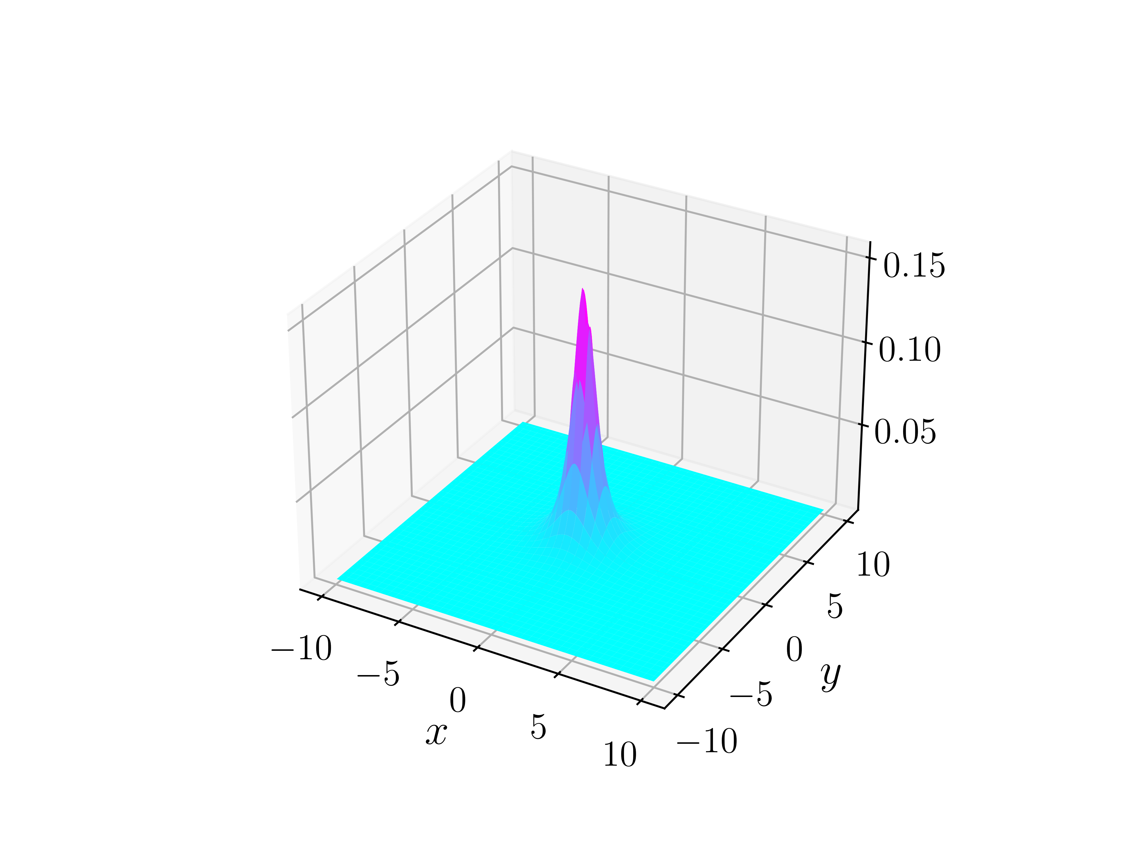
We now study the convergence of the numerical steady state to the profile (4.11) as the size of the domain grows. Unlike the one-dimensional test, the two-dimensional analysis can be performed setting $\alpha=1$ exactly. Figure 13 shows the ${L^{1}}(\Omega)$ distance between the numerical steady state of the Lévy-Fokker-Planck equation ( $\alpha=1$ , $\Delta x=\Delta y=2R/2^{8}$ , $\Delta t=0.1$ ) on $\Omega=(-R,R)^{2}$ , for various values of $R$ , and the explicit steady state (4.11). As in the one-dimensional case, the error decreases as $R$ tends to infinity.

4.2.2 Convergence of steady states

We verify the order of convergence of the dimensionally split scheme. As in one dimension, we fix the domain size and compute the steady state of the Lévy-Fokker-Planck equation (1.2) for various values of $\alpha$ . Figure 14 shows the ${L^{1}}(\Omega)$ and ${L^{2}}(\Omega)$ distance between numerical steady states ( $R=20$ , $\Delta t=\Delta x=\Delta y=2R/2^{n}$ for $5\leq n\leq 8$ ) computed with scheme (3.11) on $\Omega=(-R,R)^{2}$ as the mesh size is halved. The order of the scheme appears slightly less than one; this might be a consequence of the dimensional splitting. Noticeably, the convergence is initially very slow when the fractional order is close to zero.

4.2.3 Long-time asymptotics

To conclude, we study the rate of convergence of the numerical solution of the Lévy-Fokker-Planck equation (1.2) to the corresponding steady states. Figure 15 shows the ${L^{1}}(\Omega)$ and ${L^{2}}(\Omega)$ distances of the numerical solution ( $R=20$ , $\Delta x=\Delta y=0.15$ , $\Delta t=0.08$ ) on $\Omega=(-R,R)^{2}$ for various fractional orders to their asymptotic steady states as a function of time. Perhaps due to the highly symmetric initial data, the numerical solutions show an improved rate of convergence ( $e^{-2t}$ ) towards the steady state with respect to the result of [24] ( $e^{-\alpha t}$ ). This acceleration phenomena due to symmetry of the datum is well-documented, as it has been observed also in the classical Fokker-Planck setting [7], as well as in the porous medium equation [14].

Acknowledgements

This work was supported by the Advanced Grant Nonlocal-CPD (Nonlocal PDEs for Complex Particle Dynamics: Phase Transitions, Patterns and Synchronization) of the European Research Council Executive Agency (ERC) under the European Union’s Horizon 2020 research and innovation programme (grant agreement No. 883363). RB and JAC were also supported by the EPSRC grant numbers EP/T022132/1. JAC was also partially supported by EP/V051121/1. DGC was partially supported by RYC2022-037317-I and PID2021-127105NB-I00 from the Spanish Government. Part of this work was done during the visit of SF as master student from University of Trento by the Erasmus+ programme.

Appendix: A Second Order Discretisation

The discretisation of the advection terms described in Section 3 is only accurate to first order. However, the discretisation of the fractional diffusion term is second-order accurate, as discussed in Remark 3.3. In order to verify this, the validation tests of Section 4 employ a higher order scheme for the advection part. The discretisation of choice is classical: upwind with a minmod limiter [30, 31], which has been used successfully for generalised Fokker-Planck equations [15, 5]. For the sake of self-consistency, we detail here the one-dimensional discretisation.

The definition of the diffusive flux $F^{\textrm{dif}}_{i+\frac{1}{2}}(t)$ given in (3.3e) is not modified. Similarly, the advective velocity $v_{i+\frac{1}{2}}$ is kept as given in (3.3d). The only alteration takes place in the advective flux $F^{\textrm{ad}}_{i+\frac{1}{2}}(t)$ ; the first-order upwind formula (3.3c) is replaced by

\displaystyle F^{\textrm{ad}}_{i+\frac{1}{2}}(t)

\displaystyle=\bar{\rho}^{E}_{i}(t)(v_{i+\frac{1}{2}})^{+}+\bar{\rho}^{W}_{i+1}(t)(v_{i+\frac{1}{2}})^{-}.

(A.1)

These east and west values are computed from a piecewise linear reconstruction:

\displaystyle\bar{\rho}^{E}_{i}(t)=\bar{\rho}_{i}(t)+\frac{\Delta x}{2}\mathrm{d}\bar{\rho}_{i}(t),\quad\bar{\rho}^{W}_{i}(t)=\bar{\rho}_{i}(t)-\frac{\Delta x}{2}\mathrm{d}\bar{\rho}_{i}(t).

(A.2)

The discrete gradient $\mathrm{d}\bar{\rho}_{i}$ is defined as

\displaystyle\mathrm{d}\bar{\rho}_{i}(t)=\minmod\left(\frac{\bar{\rho}_{i}-\bar{\rho}_{i-1}}{\Delta x},\frac{\bar{\rho}_{i+1}-\bar{\rho}_{i-1}}{2\Delta x},\frac{\bar{\rho}_{i+1}-\bar{\rho}_{i}}{\Delta x}\right),

(A.3)

where

\displaystyle\minmod(a,b,c)\coloneqq\begin{cases}\min\{a,b,c\}&\text{if }a,b,c>0,\\ \max\{a,b,c\}&\text{if }a,b,c<0,\\ 0&\text{otherwise}.\end{cases}

(A.4)

References

[1] N. Abatangelo, D. Gómez-Castro, and J. L. Vázquez. Singular boundary behaviour and large solutions for fractional elliptic equations. Journal of the London Mathematical Society, 107:568–615, 2023.
[2] N. Abatangelo, D. Gómez-Castro, and J. L. Vázquez. Singular boundary behaviour and large solutions for fractional elliptic equations. Journal of the London Mathematical Society, 107(2):568–615, 2023.
[3] G. Acosta and J. P. Borthagaray. A fractional Laplace equation: Regularity of solutions and finite element approximations. SIAM Journal on Numerical Analysis, 55(2):472–495, jan 2017.
[4] M. Ainsworth and C. Glusa. Towards an efficient finite element method for the integral fractional Laplacian on polygonal domains. In Contemporary Computational Mathematics - A Celebration of the 80th Birthday of Ian Sloan, pages 17–57. Springer International Publishing, 2018.
[5] R. Bailo, J. A. Carrillo, and J. Hu. Fully discrete positivity-preserving and energy-dissipating schemes for aggregation-diffusion equations with a gradient-flow structure. Commun. Math. Sci., 18(5):1259–1303, Sept. 2020.
[6] R. Bailo, J. A. Carrillo, H. Murakawa, and M. Schmidtchen. Convergence of a fully discrete and energy-dissipating finite-volume scheme for aggregation-diffusion equations. Math. Models Methods Appl. Sci., 30(13):2487–2522, Nov. 2020.
[7] J.-P. Bartier, A. Blanchet, J. Dolbeault, and M. Escobedo. Improved intermediate asymptotics for the heat equation. Appl. Math. Lett., 24(1):76–81, 2011.
[8] P. Biler and G. Karch. Generalized fokker-planck equations and convergence to their equilibria. Banach Center Publ., 60:307–318, 2003.
[9] R. M. Blumenthal and R. K. Getoor. Some theorems on stable processes. Trans. Amer. Math. Soc., 95(2):263–273, 1960.
[10] A. Bonito, J. P. Borthagaray, R. H. Nochetto, E. Otárola, and A. J. Salgado. Numerical methods for fractional diffusion. Comput. Vis. Sci., 19(5-6):19–46, mar 2018.
[11] N. Bournaveas and V. Calvez. The one-dimensional Keller-Segel model with fractional diffusion of cells. Nonlinearity, 23(4):923–935, 2010.
[12] H. Brezis. Functional Analysis, Sobolev Spaces and Partial Differential Equations. Springer, New York, 2010.
[13] C. Bucur. Some observations on the green function for the ball in the fractional Laplace framework. Commun. Pure Appl. Anal., 15(2):657–699, jan 2016.
[14] J. Carrillo, M. Di Francesco, and G. Toscani. Strict contractivity of the 2-wasserstein distance for the porous medium equation by mass-centering. Proc. Amer. Math. Soc., 135(2):353–363, 2007.
[15] J. A. Carrillo, A. Chertock, and Y. Huang. A finite-volume method for nonlinear nonlocal equations with a gradient flow structure. Commun. Comput. Phys., 17(1):233–258, 2015.
[16] J. A. Carrillo, F. Filbet, and M. Schmidtchen. Convergence of a finite volume scheme for a system of interacting species with cross-diffusion. Numer. Math., 145(3):473–511, 2020.
[17] J. Cayama, C. M. Cuesta, and F. de la Hoz. A pseudospectral method for the one-dimensional fractional laplacian on $\mathbb{R}$ . Appl. Math. Comput., 389:125577, 2021.
[18] N. Cusimano, F. del Teso, L. Gerardo-Giorda, and G. Pagnini. Discretizations of the spectral fractional Laplacian on general domains with Dirichlet, Neumann, and Robin boundary conditions. SIAM J. Numer. Anal., 56(3):1243–1272, 2018.
[19] N. De Nitti and S. Sakaguchi. The stationary critical points of the fractional heat flow. Preprint arXiv: 2212.05383, 2022.
[20] F. del Teso. Finite difference method for a fractional porous medium equation. Calcolo, 51(4):615–638, 2014.
[21] E. Di Nezza, G. Palatucci, and E. Valdinoci. Hitchhiker’s guide to the fractional Sobolev spaces. Bull. des Sci. Math., 136(5):521–573, 2012.
[22] C. Escudero. The fractional Keller-Segel model. Nonlinearity, 19(12):2909–2918, 2006.
[23] R. Estrada and R. P. Kanwal. Singular Integral Equations. Birkhäuser Boston, 2000.
[24] I. Gentil and C. Imbert. The Lévy–Fokker–Planck equation: $\phi$ -entropies and convergence to equilibrium. Asymptot. Anal., 59(3-4):125–138, 2008.
[25] Y. Huang and A. Oberman. Numerical methods for the fractional Laplacian: A finite difference-quadrature approach. SIAM J. Numer. Anal., 52(6):3056–3084, 2014.
[26] K. Ito and F. Kappel. The trotter-kato theorem and approximation of pdes. Math. Comp., 67(221):21–44, 1998.
[27] T. Kato. Trotter’s product formula for an arbitrary pair of self-adjoint contraction semigroup. Topics in Func. Anal., Adv. Math. Suppl. Studies, 3:185–195, 1978.
[28] M. Kwasnicki. Ten equivalent definitions of the fractional laplace operator. Fract. Calc. Appl. Anal., 20(1):7–51, 2017.
[29] L. Lafleche and S. Salem. Fractional Keller-Segel equation: global well-posedness and finite time blow-up. Commun. Math. Sci., 17(8):2055–2087, 2019.
[30] R. J. LeVeque. Numerical Methods for Conservation Laws. Birkhäuser Basel, 1990.
[31] R. J. LeVeque. Finite Volume Methods for Hyperbolic Problems. Cambridge Texts in Applied Mathematics. Cambridge University Press, 2002.
[32] D. Li and J. Rodrigo. Finite-time singularities of an aggregation equation in $\mathbb{R}^{n}$ with fractional dissipation. Comm. Math. Phys., 287(2):687–703, 2009.
[33] A. Lischke, G. Pang, M. Gulian, F. Song, C. Glusa, X. Zheng, Z. Mao, W. Cai, M. M. Meerschaert, M. Ainsworth, and G. E. Karniadakis. What is the fractional Laplacian? a comparative review with new results. J. Comput. Phys., 404:109009, mar 2020.
[34] Z. Mao and J. Shen. Hermite spectral methods for fractional PDEs in unbounded domains. SIAM J. Sci. Comput., 39(5):A1928–A1950, 2017.
[35] R. H. Nochetto, E. Otárola, and A. J. Salgado. A PDE approach to fractional diffusion in general domains: a priori error analysis. Found. Comput. Math., 15(3):733–791, 2015.
[36] Y. Saad. Iterative Methods for Sparse Linear Systems. Society for Industrial and Applied Mathematics, Jan. 2003.
[37] C. Sheng, J. Shen, T. Tang, L.-L. Wang, and H. Yuan. Fast Fourier-like mapped Chebyshev spectral-Galerkin methods for PDEs with integral fractional Laplacian in unbounded domains. SIAM J. Numer. Anal., 58(5):2435–2464, 2020.
[38] E. M. Stein. Singular Integrals and Differentiability Properties of Functions. Princeton University Press, 1970.
[39] H. F. Trotter. On the product of semi-groups of operators. Proc. Amer. Math. Soc., 10(4):545–551, 1959.
[40] E. Valdinoci. From the long jump random walk to the fractional Laplacian. SeMA J. Boletín la Soc. Española Matemática Apl., 49:1–7, 2009.
[41] W. Xu and L. Wang. An asymptotic preserving scheme for Lévy-Fokker-Planck equation with fractional diffusion limit. Preprint arXiv: 2103.08848, 2021.

A Finite-Volume Scheme for Fractional Diffusion on Bounded Domains

Abstract

1 Introduction

2 A new fractional Laplacian in bounded domains

Theorem 2.1.

Proof.

3 Numerical schemes

3.1 One dimension

Remark 3.1 (Linearity).

Remark 3.2 (Symmetry).

Remark 3.3 (Higher order advection).

Remark 3.4 (Time discretisation).

Remark 3.5 (The range α≤1\alpha\leq 1).

3.2 Two dimensions

3.2.1 Dimensional Splitting

Remark 3.6 (Sweeping dimensional splitting).

4 Numerical experiments

4.1 One dimension

4.1.1 Fractional diffusion

4.1.2 Singular behaviour at the boundary

4.1.3 Steady states as a function of domain size

4.1.4 Convergence of steady states

4.2 Two dimensions

4.2.1 Steady states as a function of domain size

4.2.2 Convergence of steady states

4.2.3 Long-time asymptotics

Acknowledgements

Appendix: A Second Order Discretisation

References

A Finite-Volume Scheme for
Fractional Diffusion on Bounded Domains

Remark 3.5 (The range $\alpha\leq 1$ ).