Topological and geometric analysis of cell states in single-cell transcriptomic data

To explore the structure-function relationship underlying single-cell data, we develop scGeom, a tool that characterizes the geometric and topological properties of cell networks and gene networks and relate them to the biological properties of cells (Fig. 1). The single-cell data is first preprocessed following the common pipelines of normalization, highly variable gene selection and PCA dimension reduction. A cell network denoted by $G_{\mathrm{c}}=(V_{\mathrm{c}},E_{\mathrm{c}})$ is then constructed by building a $k$-nearest neighbor graph with respect to Euclidean distance of the PCA embeddings. On $G_{\mathrm{c}}$, a graph curvature is computed for each edge using a discretization of Ricci curvature on graphs, the Ollivier-Ricci curvature (ORC)[27] which measures the divergence of local geometry from the Euclidean space. Specifically, for the edge $e_{ij}\in E_{\mathrm{c}}$, ORC examines the difference between the edge length $e_{ij}$ and the distance between neighborhoods of $v_{i}$ and $v_{j}$ by optimal transport with shortest path distance as the ground cost. The curvatures on nodes are then defined by summing over the corresponding edges. A cell within a community or between communities is likely to have a positive or negative graph curvature respectively, analogous to scalar curvature in Riemannian geometry.

The topological structures are characterized by persistent homology[20, 19]. The structure of the network is represented by a growing sequence of simplicial complexes that generalize graphs to higher dimensions. This sequence is called a filtration which captures the structural features at various scales compared to using one fixed graph or simplicial complex. Along the filtration, persistent homology tracks the appearances and disappearances of $k$-dimensional holes and their persistence through the filtration. For example, the $0$, $1$, and $2-$dimensional holes correspond to connected components, loops, and voids. Given a graph or point cloud, persistent homology outputs collections of persistence intervals, also called persistence diagrams, $\mathrm{Dgm}_{k}=[b_{i},d_{i})_{i=1}^{n^{(k)}}$ representing the filtration values corresponding to the appearance ($b_{i}$) and the disappearance ($d_{i}$) of the $k$th homology groups associated to the $k$-dimensional holes. Details of graph curvature and persistent homology are discussed in Sections 3.1 and 3.2. For each cell in the cell network, persistent homology is computed for its local neighborhood. The graph curvature $\kappa$ and featurizations of the persistence diagram such as the total persistence $\sum_{i}(d_{i}-b_{i})$ are used to distinguish cells in the transition and stable states (Fig. 1b).

A cell-specific gene network[11], $G_{\mathrm{g}}$ is constructed to reveal higher-order properties of cells in addition to the first-order gene expression levels. Persistence diagrams are computed for $G_{\mathrm{g}}^{i}$ of cell $i$ using filtrations such as edge-weighted Vietoris-Rips complex, resulting in persistence diagrams $\mathrm{Dgm}_{k}(G_{\mathrm{g}}^{i})$. We then turn the persistence diagrams into features including persistence images that fit kernels to the $\mathrm{Dgm}_{k}$ regarded as point clouds, Betti curves that count the number of homology groups at every filtration value, and various statistics of $\mathrm{Dgm}_{k}$ such as total persistence and longest persistence. These features are then used to analyze the pluripotency or developmental potency of cells and fed to machine learning methods together with gene expression features for predicting cell types (Fig. 1c). Details of the methods and preprocessing of data can be found in Section 3.

We first analyzed a scRNA-seq data of myelopoiesis which captures several transitional intermediate states during differentiation of blood cells [28]. In this dataset, two relatively unstable states, a multi-lineage state and a monocyte intermediate state were identified by the original study using the ICGS approach[28] and another analysis of the dataset using a physics-based modeling tool MuTrans[9] (Fig. 2a). Further, the MuTrans analysis constructed a differentiation landscape and identified transition cells between states depicted by the entropy of probability score assigned to each state (Fig. 2a). Here, based on $k$-nearest neighbors graphs of cells using the PCA embedding, we computed the Ollivier-Ricci curvature for each cell. We also computed topological features of each cell including local persistent homology on a neighborhood graph centered at the cell and the relative persistent homology of the global structure relative to a small neighborhood of the cell. The local persistent homology captures the multiscale and multidimensional structural characteristics of the local structure centered at each cell and the resulting persistence diagrams are turned into features by computing the total persistence and the persistence entropy[29]. The relative persistent homology examines the significance of a cell in defining the global structure of the dataset. The resulting persistence diagrams are described by computing the Wasserstein distance between the relative persistence diagram and the regular persistence diagram of the whole dataset. These geometric and topological features were able to highlight both the relatively unstable cell states and the transition cells between states (Fig. 2b).

We then analyzed a single-cell dataset of induced pluripotent stem cells (iPSCs) taken at several real time points[30] (Fig. 2c). This dataset depicts two major transition events, epiblast (EPI) to primitive-streak (PS) cells and PS to mesenchymal (M) and endodermal (En) cells. Utilizing biological knowledge, the original study[30] projected these two transition events to happen around day 1.5 and day 2.5, respectively. Here, we perform an unbiased analysis without using any prior knowledge. We computed the graph curvature and local persistent homology on the PCA embedding and found a significant decrease in curvature and an increase in total persistence at day 1.5 and day 2.5. A smaller curvature indicates bridges between stable states. For topology, more significant topological features, for example, higher total persistence, reflect divergence from trivial structures and thus reveal the transition processes.

In addition to examining the structures of cell networks, we further explore the relation between cell states and the structures of gene networks. A prior knowledge-based gene network[13] was assigned to each cell where the node weights were determined by the gene expression levels in the corresponding cell. For each cell, persistent homology was computed on this node-weighted gene network using vertex-based clique complex filtration where the edge filtration value is determined as the smaller weights of its two nodes.

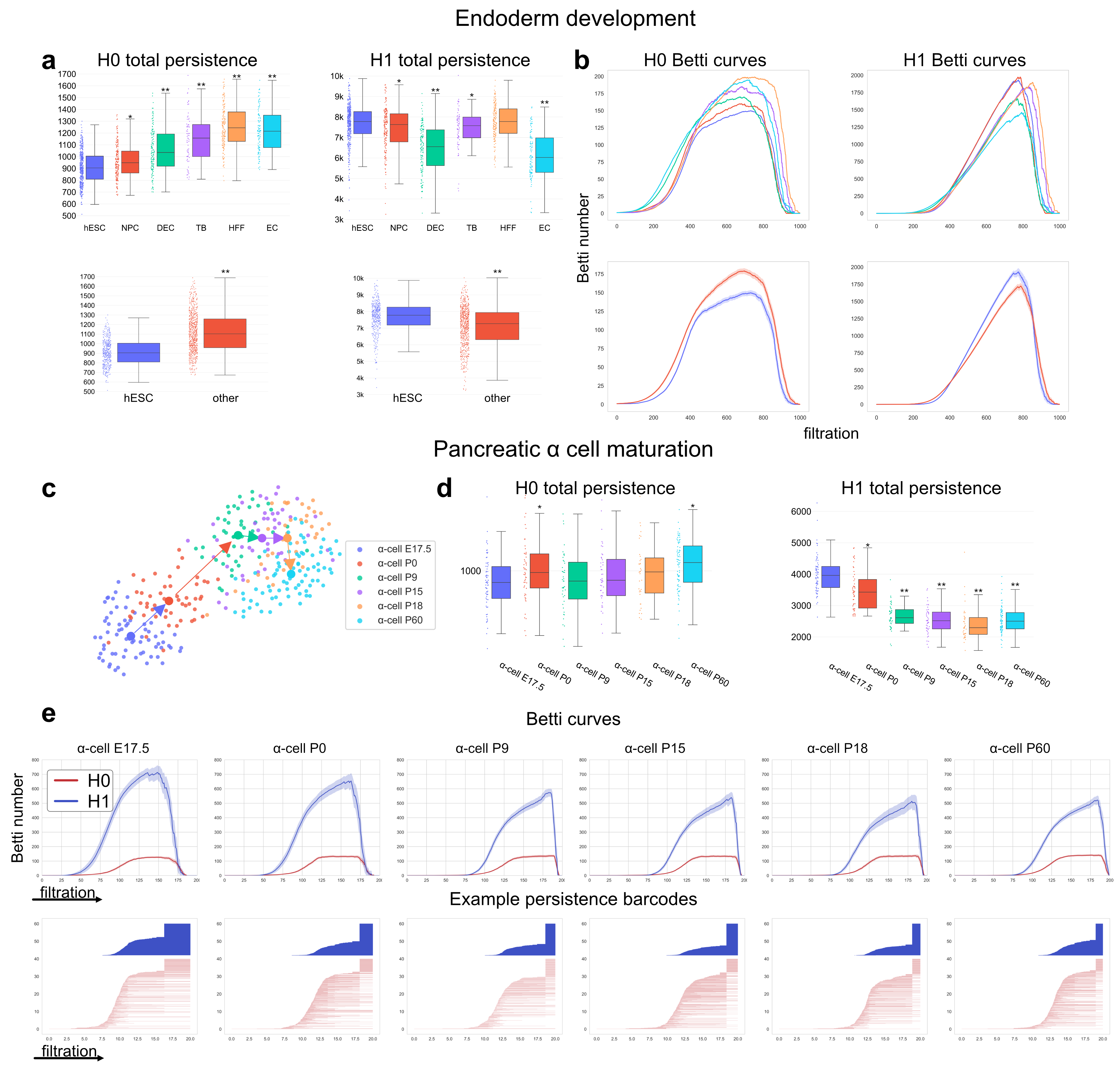
We first analyzed a scRNA-seq data of human definitive endoderm development[31]. In this dataset, the human embryonic stem cells (hESC) are pluripotent cells that differentiate into several lineage-specific progenitors. Evaluating the persistent homology of cells at each state, we observe an increase in $H_{0}$ total persistence and a decrease of $H_{1}$ total persistence along the differentiating progress (Fig. 3a). The $H_{0}$ and $H_{1}$ persistent homology captures connected components and loop-like structures which indicates that the gene network of pluripotent cells tends to have less isolated components (shorter $H_{0}$ persistence) and differentiated cells tend to be active in a localized part of the gene network (shorter $H_{1}$ persistence). Comparing hESC cells with all other cells also shows significantly lower $H_{0}$ persistence and higher $H_{1}$ persistence in hESC cells (Fig. 3a). The Betti curves summarize the number of connected components ($H_{0}$) and $1$-dimensional holes or loops ($H_{1}$) at every filtration value which also show that hESC cells have fewer disconnected parts and larger-scale loops with more coverage of the gene network(Fig. 3b).

We also analyzed a scRNA-seq data of mouse pancreatic $\alpha$ cell maturation tracking along one cell lineage[32]. In this dataset, scRNA-seq experiments were performed for pancreatic $\alpha$ cells at different developmental stages including embryonic data 17.5 (E17.5) and postnatal day P0, P9, P15, P18, and P60 (Fig. 3c). During the maturation, we also observed a similar pattern with increasing $H_{0}$ persistence and decreasing $H_{1}$ persistence (Fig. 3d). The observation is further confirmed in the Betti curves and persistence barcodes of example cells from each maturation stage (Fig. 3e). Together, these examples demonstrate that the topological signatures of gene networks reflect the developmental potential of cells.

Having shown the utility of topological and geometric structures in single-cell data for analyzing transition cells and developmental potential, here, we explore the usage of these structures in the general task of cell type annotations. We used a mouse brain dataset and a mouse kidney dataset from the cell type annotation subtask in a benchmarking resource[33] with pre-defined train/test splittings. In this task, a predictive model is trained on annotated data to predict cell types from their gene expression profiles.

We performed two topological characterizations of the gene networks for each cell. First, a cell-specific gene network (CSN) is constructed using a correlation-based approach[11] which results in an edge-weighted gene network for each cell. The CSNs were generated on processed data using the preprocessing pipeline of SingleCellNet[34] to select the marker genes of each cell type. Then, we computed persistent homology using an inverse Vietoris-Rips complex-based filtration which adds $1$-simplexes and subsequently the higher dimensional simplices with large edge weights first. Second, we utilize a prior knowledge-based gene network (SCENT[13]) on the single-cell datasets without gene filtering. The same gene network structure is assigned to each cell but with different node weights assigned from gene expression levels. In this case, persistent homology was computed based on a vertex-based clique-complex filtration where $0$-simplices and subsequent higher dimensional simplices with higher weights are added first. The total persistence and persistence entropy[29] of the resulting persistence diagrams were used as topological features for the cells.

In both benchmarks, the classification performance is improved with the additional topological features evaluated by accuracy, balanced accuracy, and macro-average precision and recall (Fig. 4. The Betti curves and persistence barcodes of several example cells demonstrate the differences in the topological signature of gene networks across different cell types (Fig. 4c,f). In the brain dataset, interestingly, we observe significantly longer persistence in the $H_{1}$ persistence barcodes of neuron cells compared to other brain cells indicating a broader coverage of gene network and diverse functions. This observation agrees with the diverse signals sent and functions controlled by neuron cells[35].

Given a metric, the Ricci curvature describes how much the local geometry on a manifold differs from that of the ordinary Euclidean space. It measures intrinsic local properties of manifolds such as divergence of geodesics and meeting probabilities of coupled random walks. Several constructions have been introduced to define Ricci curvature on graphs, such as Ollivier-Ricci[36, 27, 37] curvature. For an edge connecting two nodes, Ollivier-Ricci curvature (ORC) measures the difference between the edge distance between the nodes and the optimal transport distance between the nodes’ neighborhoods. Let $G=(V,E)$ be an undirected graph with vertices $V=\{v_{i}\}_{i=1}^{n}$ and edges $E=\{e_{ij}\}_{1\leq i,j\leq n}$, a measure is defined for each node describing its local neighborhood such that

where $N(v_{i})$ is the set of nodes connected to $v_{i}$ in $G$ and $\alpha\in[0,1]$ is the parameter annotating the weight on the center node. The ORC $\kappa_{ij}$ between $v_{i}$ and $v_{j}$ is then defined to be

where $d()$ is the shortest path distance on $G$ and $d_{W}$ is the Wasserstein distance with $d()$ as the ground metric. Specifically, an optimal transport problem is solved, $d_{W}(m_{v_{i}},m_{v_{j}})=\inf\limits_{\pi\in\Pi(m_{v_{i}},m_{v_{j}})}<\pi,C>_{F}$ with $C_{ij}=d(v_{i},v_{j})$ and $\Pi(a,b)=\{\pi\in\mathbb{R}_{+}^{n\times n}|\pi\mathbf{1}=a,\pi^{T}\mathbf{1}=b\}$.

Persistent homology[20, 19, 21] provides a comprehensive multiscale topological characterization by tracking the appearance and disappearance of homology groups through a filtration which is a growing sequence of simplicial complexes defined on the data. An abstract $k$-simplex is a set of $k+1$ vertices denoted $\sigma^{k}=\{v_{0},\cdots,v_{k}\}$. Any subset $\sigma^{\prime}\subseteq\sigma^{k}$ is called a face of $\sigma^{k}$. A simplicial complex $K$ is a set of simplices satisfying that all faces of any simplex in $K$ is also in $K$ and the intersection of any pair of simplices is either empty or a common face of the two. A filtration of a simplicial complex $K$ is a nested sequence of its subcomplexes, $\emptyset=K^{0}\subset K^{1}\subset\cdots\subset K^{n}=K$. A $k$-chain of a simplicial complex $K$ denoted by $c_{k}$ is a formal sum of $k$-simplices in $K$ with coefficients from a chosen set, for example, $\mathbb{Z}_{2}$. The $k$-chains of $K$ forms a group called the $k$th chains group denoted by $C_{k}(K)$. The $k$-chains are connected by a linear boundary operator $\partial_{k}:C_{k}(K)\rightarrow C_{k-1}(K)$ such that $\partial_{k}(\sigma^{k})=\sum\limits_{i=0}^{k}(-1)^{i}\hat{\sigma}^{k-1}_{i}$ where $\hat{\sigma}^{k-1}_{i}$ is a face of $\sigma^{k}$ obtained by removing vertex $i$. Based on the boundary operator, two groups are defined, the kernel of $\partial_{k}$, $Z_{k}(K)=\mathrm{ker}(\partial_{k})$ whose elements are called $k$-cycles and the image of $\partial_{k+1}$ denoted by $B_{k}(K)$ also called the $k$th boundary group. The $k$th homology group is then defined as the quotient group $H_{k}(K)=Z_{k}(K)/B_{k}(K)$ whose rank $\mathrm{rank}(H_{k}(K))=\mathrm{rank}(B_{k}(K))-\mathrm{rank}(B_{k}(K))$ is also the $k$th Betti number of $K$ representing the number of $k$-dimensional holes in $K$. On the filtration of $K$, the $p$-persistent $k$th homology group is defined to be $H_{k}^{p}(K^{i})=Z_{k}(K^{i})/(B_{k}(K^{i+p})\cap Z_{k}(K^{i}))$ which intuitively represents a topological feature observed at filtration step $i$ and persists through step $i+p$. An equivalence class in $H_{k}(K^{i})$ persisting through $H_{k}(K^{j})$ but is not present in $H_{k}(K^{i-1})$ or $H_{k}(K^{j+1})$ result in a persistence pair conveniently represented as the interval $[x_{i},x_{j})$ often called the birth-death pairs where $x_{i}$ and $x_{j}$ are the filtration values of $K^{i}$ and $K^{j}$ respectively. Persistent homology characterization of a dataset results in a collection of such birth-death pairs and is often visualized as persistence barcodes (plotting each pair as a horizontal bar whose two endpoints correspond to the birth and death values) or persistence diagrams (plotting each pair as a point in 2D).

The raw single-cell data was first preprocessed by normalizing total counts in every cell and log1p transformation ($\log(1+x)$). Principal component analysis is then performed with the selected highly variable genes. A $k$-nearest neighbor graph is constructed based on the Euclidean distance in the space of top principal components. The ORC is computed on this cell network with the $\alpha$ parameter (the portion of mass assigned to the center cell when determining a mass distribution representing the neighborhood of the cell) set to 0.5. The preprocessing was performed using the Scanpy package[38].

To characterize the topological structures of the cell network for each cell, we use two approaches, a local persistent homology and a relative persistent homology. The local persistent homology aims to capture the local structure surrounding a cell in the cell network. Here, we adopt a simple approach by computing the regular persistent homology on a sub-network surrounding a cell defined by either the top $k$ nearest neighbors or a distance cutoff. This approach has been shown effective in capturing local topological structures in various applications such as biomolecular structure analysis[24]. The relative persistent homology, on the other hand, captures the significance of a cell or the neighborhood of a cell in assembling the global structure of the dataset. Let $\emptyset=K^{0}\subset K^{1}\subset\cdots\subset K^{n}=K$ be a filtration of the whole dataset. For cell $i$, we define a subcomplex $L_{i}$ which contains only this cell or its local neighborhood on the network. Then, relative persistent homology examines the homology on the relative chain groups which are quotient groups $C_{k}(K^{j})/C_{k}(K^{j}\cap L_{i})$. The impact of cell $i$ on assembling the global dataset structure is then quantified by computing the Wasserstein distance between the relative persistent homology diagrams and the regular persistent homology diagram of the whole dataset. For both approaches, we used the Vietoris-Rips filtration with the Euclidean distance between cells in their PCA embeddings.

Here, we consider two types of gene networks, a cell-specific gene network in the form of edge-weighted networks and a prior knowledge-based gene network in the form of node-weighted networks.

The package CSN[11] is used to construct a cell-specific gene network for each cell on the top highly variable genes in the dataset. The core statistic in this method evaluates the local association between each gene pair for every cell. Specifically, for cell $k$ and genes $x$ and $y$, $\rho_{xy}^{(k)}=n_{xy}^{(k)}/n-(n_{x}^{(k)}/n)(n_{y}^{(k)}/n)$, where $n$ is the total number of cells. The parameter $n_{x}^{(k)}$ is predefined and induces an interval $I_{x}^{(k)}$ of the expression of gene $x$ in the top $n_{x}^{(k)}$ cells whose gene $x$ expression is the closest to cell $k$. Similarly, an interval for gene $y$, $I_{y}^{(k)}$ is determined by $n_{y}^{(k)}$. Then $n_{x}y^{(k)}$ counts the number of cells in whose expressions of gene $x$ and gene $y$ both fall in the two intervals, respectively. Here, we used the top 1000 highly variable genes and used the default parameter values in the CSN method[11] with $n_{x}^{(k)}=n_{y}^{(k)}=0.1n$ and significant level set to $0.01$. The constructed cell-specific gene networks are edge-weighted networks. Denoting the network of a cell by $G=(V,E,W^{(e)})$, we compute persistent homology with the Vietoris-Rips filtration

The filtration is computed from $\delta=\delta_{max}=\max\{W^{(e)}\}$ to $\delta=0.$ The resulting persistence pairs $[b_{i},d_{i})_{i}$ are transformed to $[\delta_{max}-b_{i},\delta_{max}-d_{i})_{i}$.

For the prior knowledge-based gene network, a base network is first assigned to each cell and the gene expression levels in each cell are assigned as node weights. Denoting the network of a cell by $G=\{V,E,W^{(v)}\}$, persistent homology is computed using the vertex-based clique complex filtration

Similar to the edge-weighted network, the filtration is computed from $\delta=\delta_{max}=\max\{W^{(v)}\}$ to $\delta=0$. The resulting persistence pairs $[b_{i},d_{i})_{i}$ are also transformed to $[\delta_{max}-b_{i},\delta_{max}-d_{i})_{i}$. The log1p transformed gene expression levels are used to assign node weight and the full dataset without gene filtering is used with the knowledge-based gene network.

The computation of filtration and persistent homology was based on the packages Gudhi[39], Dionysus2[40], and Ripser[41].

For dimension $k$, persistent homology computation results in a collection of $n^{(k)}$ persistence pairs $[b^{(k)}_{i},d^{(k)}_{i})_{i=1}^{n^{(k)}}$ where $b^{(k)}_{i}$ and $d^{(k)}_{i}$ are the filtration values corresponding to the birth and death of a topological feature ($k$-dimensional holes). Several summaries and features are derived from the persistence pairs. Total persistence describes the overall significance of topological features in the data and is computed as $L^{(k)}=\sum_{i=1}^{n}(\bar{d}^{(k)}_{i}-b^{(k)}_{i})$ where $\bar{d}^{(k)}_{i}=\min\{d^{(k)}_{i},\delta_{max}\}$. Persistence entropy[29] describes the heterogeneity of persistence similar to Shannon entropy and is stable with respect to small perturbations in the input space. Specifically, it is computed as $E^{(k)}=-\sum_{i=1}^{n^{(k)}}\frac{l^{(k)}_{i}}{L^{(k)}}\log_{2}(\frac{l^{(k)}_{i}}{L^{(k)}})$ where $l^{(k)}_{i}=\bar{d}^{(k)}_{i}-b^{(k)}_{i}$ is the persistence of the $i$th pair. In addition to global summaries, Betti curves describe the structural changes along the filtration and are convenient for illustrating the average behavior of a group of persistence barcodes. For a filtration value $\delta$, the $k$-dimensional Betti curve is computed as $BC^{(k)}(\delta)=\#\{[b^{(k)}_{i},d^{(k)}_{i}):\delta\in[b^{(k)}_{i},d^{(k)}_{i})\}$. Betti curve is computed on a discretization of the filtration interval $[0,\delta_{max}]$. The Gudhi package[39] was used to compute the persistence entropy and Betti curves.

In the application of cell type classification, the implementation of random forest model in scikit-learn package[42] was used with 5000 trees and "class_weight" parameter set to "balanced". All other parameters are set to default values. The classification results on the testing set were evaluated using accuracy: $(1/N)\sum_{i}1(\hat{y}_{i}=y_{i})$; balanced accuracy (adjusted): $\left(1/\sum_{i}\frac{1}{N_{c(i)}}\right)\sum_{i}1(\hat{y}_{i}=y_{i})\frac{1}{N_{c(i)}}-\frac{1}{C}$; precision (macro-average): $\frac{1}{C}\sum_{c=1}^{C}\frac{|\hat{Y}_{c}\cap Y_{c}|}{|\hat{Y}_{c}|}$; and recall (macro-average): $\frac{1}{C}\sum_{c=1}^{C}\frac{|\hat{Y}_{c}\cap Y_{c}|}{|Y_{c}|}$. Here, $N$ is the total number of samples, $N_{c(i)}$ is the number of samples of the same class as sample $i$ in the ground truth, $y_{i}$ is the true label of sample $i$, $\hat{y}_{i}$ is the predicted label of sample $i$, $C$ is the number of classes, $Y_{c}$ is the set of samples of class $c$ in ground truth, $\hat{Y}_{c}$ is the set of sample predicted to be class $c$, and $1()$ is the indicator function.

References

- [1] Valentine Svensson, Roser Vento-Tormo, and Sarah A Teichmann. Exponential scaling of single-cell rna-seq in the past decade. Nature protocols, 13(4):599–604, 2018.
- [2] Malte D Luecken and Fabian J Theis. Current best practices in single-cell rna-seq analysis: a tutorial. Molecular systems biology, 15(6):e8746, 2019.
- [3] Michael Ashburner, Catherine A Ball, Judith A Blake, David Botstein, Heather Butler, J Michael Cherry, Allan P Davis, Kara Dolinski, Selina S Dwight, Janan T Eppig, et al. Gene ontology: tool for the unification of biology. Nature genetics, 25(1):25–29, 2000.
- [4] Yutong Sha, Shuxiong Wang, Peijie Zhou, and Qing Nie. Inference and multiscale model of epithelial-to-mesenchymal transition via single-cell transcriptomic data. Nucleic acids research, 48(17):9505–9520, 2020.
- [5] Xiaoying Zheng, Suoqin Jin, Qing Nie, and Xiufen Zou. scrcmf: Identification of cell subpopulations and transition states from single-cell transcriptomes. IEEE Transactions on Biomedical Engineering, 67(5):1418–1428, 2019.
- [6] Lingxue Zhu, Jing Lei, Lambertus Klei, Bernie Devlin, and Kathryn Roeder. Semisoft clustering of single-cell data. Proceedings of the National Academy of Sciences, 116(2):466–471, 2019.
- [7] Tian Lan, Gyorgy Hutvagner, Xuan Zhang, Tao Liu, Limsoon Wong, and Jinyan Li. Density-based detection of cell transition states to construct disparate and bifurcating trajectories. Nucleic Acids Research, 50(21):e122–e122, 2022.
- [8] Yanglan Gan, Cheng Guo, Wenjing Guo, Guangwei Xu, and Guobing Zou. Entropy-based inference of transition states and cellular trajectory for single-cell transcriptomics. Briefings in Bioinformatics, 23(4):bbac225, 2022.
- [9] Peijie Zhou, Shuxiong Wang, Tiejun Li, and Qing Nie. Dissecting transition cells from single-cell transcriptome data through multiscale stochastic dynamics. Nature communications, 12(1):5609, 2021.
- [10] Wenjun Kong, Yuheng C Fu, Emily M Holloway, Görkem Garipler, Xue Yang, Esteban O Mazzoni, and Samantha A Morris. Capybara: A computational tool to measure cell identity and fate transitions. Cell Stem Cell, 29(4):635–649, 2022.
- [11] Hao Dai, Lin Li, Tao Zeng, and Luonan Chen. Cell-specific network constructed by single-cell rna sequencing data. Nucleic acids research, 47(11):e62–e62, 2019.
- [12] Xuran Wang, David Choi, and Kathryn Roeder. Constructing local cell-specific networks from single-cell data. Proceedings of the National Academy of Sciences, 118(51):e2113178118, 2021.
- [13] Christopher RS Banerji, Diego Miranda-Saavedra, Simone Severini, Martin Widschwendter, Tariq Enver, Joseph X Zhou, and Andrew E Teschendorff. Cellular network entropy as the energy potential in waddington’s differentiation landscape. Scientific reports, 3(1):3039, 2013.
- [14] Andrew E Teschendorff and Tariq Enver. Single-cell entropy for accurate estimation of differentiation potency from a cell’s transcriptome. Nature communications, 8(1):15599, 2017.
- [15] Kevin A Murgas, Emil Saucan, and Romeil Sandhu. Hypergraph geometry reflects higher-order dynamics in protein interaction networks. Scientific Reports, 12(1):20879, 2022.
- [16] Larry Wasserman. Topological data analysis. Annual Review of Statistics and Its Application, 5:501–532, 2018.
- [17] Gurjeet Singh, Facundo Mémoli, Gunnar E Carlsson, et al. Topological methods for the analysis of high dimensional data sets and 3d object recognition. PBG@ Eurographics, 2:091–100, 2007.
- [18] Abbas H Rizvi, Pablo G Camara, Elena K Kandror, Thomas J Roberts, Ira Schieren, Tom Maniatis, and Raul Rabadan. Single-cell topological rna-seq analysis reveals insights into cellular differentiation and development. Nature biotechnology, 35(6):551–560, 2017.
- [19] Afra Zomorodian and Gunnar Carlsson. Computing persistent homology. In Proceedings of the twentieth annual symposium on Computational geometry, pages 347–356, 2004.
- [20] Edelsbrunner, Letscher, and Zomorodian. Topological persistence and simplification. Discrete & Computational Geometry, 28:511–533, 2002.
- [21] Herbert Edelsbrunner, John Harer, et al. Persistent homology-a survey. Contemporary mathematics, 453(26):257–282, 2008.
- [22] Ann E Sizemore, Jennifer E Phillips-Cremins, Robert Ghrist, and Danielle S Bassett. The importance of the whole: topological data analysis for the network neuroscientist. Network Neuroscience, 3(3):656–673, 2019.
- [23] Zixuan Cang and Guo-Wei Wei. Topologynet: Topology based deep convolutional and multi-task neural networks for biomolecular property predictions. PLoS computational biology, 13(7):e1005690, 2017.
- [24] Zhenyu Meng, D Vijay Anand, Yunpeng Lu, Jie Wu, and Kelin Xia. Weighted persistent homology for biomolecular data analysis. Scientific reports, 10(1):2079, 2020.
- [25] Tomasz Kaczynski, Konstantin Michael Mischaikow, and Marian Mrozek. Computational homology, volume 3. Springer, 2004.
- [26] Mehmet E Aktas, Esra Akbas, and Ahmed El Fatmaoui. Persistence homology of networks: methods and applications. Applied Network Science, 4(1):1–28, 2019.
- [27] Yann Ollivier. Ricci curvature of markov chains on metric spaces. Journal of Functional Analysis, 256(3):810–864, 2009.
- [28] Andre Olsson, Meenakshi Venkatasubramanian, Viren K Chaudhri, Bruce J Aronow, Nathan Salomonis, Harinder Singh, and H Leighton Grimes. Single-cell analysis of mixed-lineage states leading to a binary cell fate choice. Nature, 537(7622):698–702, 2016.
- [29] Nieves Atienza, Rocío González-Díaz, and Manuel Soriano-Trigueros. On the stability of persistent entropy and new summary functions for topological data analysis. Pattern Recognition, 107:107509, 2020.
- [30] Rhishikesh Bargaje, Kalliopi Trachana, Martin N Shelton, Christopher S McGinnis, Joseph X Zhou, Cora Chadick, Savannah Cook, Christopher Cavanaugh, Sui Huang, and Leroy Hood. Cell population structure prior to bifurcation predicts efficiency of directed differentiation in human induced pluripotent cells. Proceedings of the National Academy of Sciences, 114(9):2271–2276, 2017.
- [31] Li-Fang Chu, Ning Leng, Jue Zhang, Zhonggang Hou, Daniel Mamott, David T Vereide, Jeea Choi, Christina Kendziorski, Ron Stewart, and James A Thomson. Single-cell rna-seq reveals novel regulators of human embryonic stem cell differentiation to definitive endoderm. Genome biology, 17:1–20, 2016.
- [32] Wei-Lin Qiu, Yu-Wei Zhang, Ye Feng, Lin-Chen Li, Liu Yang, and Cheng-Ran Xu. Deciphering pancreatic islet cell and cell maturation pathways and characteristic features at the single-cell level. Cell metabolism, 25(5):1194–1205, 2017.
- [33] Jiayuan Ding, Hongzhi Wen, Wenzhuo Tang, Renming Liu, Zhaoheng Li, Julian Venegas, Runze Su, Dylan Molho, Wei Jin, Wangyang Zuo, et al. Dance: A deep learning library and benchmark platform for single-cell analysis. bioRxiv, pages 2022–10, 2022.
- [34] Yuqi Tan and Patrick Cahan. Singlecellnet: a computational tool to classify single cell rna-seq data across platforms and across species. Cell systems, 9(2):207–213, 2019.
- [35] Lucio M Schiapparelli, Pranav Sharma, Hai-Yan He, Jianli Li, Sahil H Shah, Daniel B McClatchy, Yuanhui Ma, Han-Hsuan Liu, Jeffrey L Goldberg, John R Yates, et al. Proteomic screen reveals diverse protein transport between connected neurons in the visual system. Cell reports, 38(4), 2022.
- [36] John Lott and Cédric Villani. Ricci curvature for metric-measure spaces via optimal transport. Annals of Mathematics, pages 903–991, 2009.
- [37] Yann Ollivier. A survey of ricci curvature for metric spaces and markov chains. In Probabilistic approach to geometry, volume 57, pages 343–382. Mathematical Society of Japan, 2010.
- [38] F Alexander Wolf, Philipp Angerer, and Fabian J Theis. Scanpy: large-scale single-cell gene expression data analysis. Genome biology, 19:1–5, 2018.
- [39] The GUDHI Project. GUDHI User and Reference Manual. GUDHI Editorial Board, 2015.
- [40] Dmitriy Morozov. Dionysus2: a c++ library for computing persistent homology, 2023.
- [41] Ulrich Bauer. Ripser: efficient computation of Vietoris-Rips persistence barcodes. J. Appl. Comput. Topol., 5(3):391–423, 2021.
- [42] F. Pedregosa, G. Varoquaux, A. Gramfort, V. Michel, B. Thirion, O. Grisel, M. Blondel, P. Prettenhofer, R. Weiss, V. Dubourg, J. Vanderplas, A. Passos, D. Cournapeau, M. Brucher, M. Perrot, and E. Duchesnay. Scikit-learn: Machine learning in Python. Journal of Machine Learning Research, 12:2825–2830, 2011.
- [43] Paul Bendich, Peter Bubenik, and Alexander Wagner. Stabilizing the unstable output of persistent homology computations. Journal of Applied and Computational Topology, 4(2):309–338, 2020.
- [44] Ippei Obayashi. Volume-optimal cycle: Tightest representative cycle of a generator in persistent homology. SIAM Journal on Applied Algebra and Geometry, 2(4):508–534, 2018.
- [45] Zixuan Cang and Guo-Wei Wei. Persistent cohomology for data with multicomponent heterogeneous information. SIAM journal on mathematics of data science, 2(2):396–418, 2020.
- [46] Hee Rhang Yoon, Robert Ghrist, and Chad Giusti. Persistent extensions and analogous bars: data-induced relations between persistence barcodes. Journal of Applied and Computational Topology, pages 1–47, 2023.
- [47] Alev Baysoy, Zhiliang Bai, Rahul Satija, and Rong Fan. The technological landscape and applications of single-cell multi-omics. Nature Reviews Molecular Cell Biology, pages 1–19, 2023.
- [48] Magnus Bakke Botnan and Michael Lesnick. An introduction to multiparameter persistence. arXiv preprint arXiv:2203.14289, 2022.