Variational Quantum Linear Solver enhanced Quantum Support Vector Machine
test is test is
Abstract
Quantum Support Vector Machines (QSVM) play a vital role in using quantum resources for supervised machine learning tasks, such as classification. However, current methods are strongly limited in terms of scalability on Noisy Intermediate Scale Quantum (NISQ) devices. In this work, we propose a novel approach called the Variational Quantum Linear Solver (VQLS) enhanced QSVM. This is built upon our idea of utilizing the variational quantum linear solver to solve system of linear equations of a least squares-SVM on a NISQ device. The implementation of our approach is evaluated by an extensive series of numerical experiments with the Iris dataset, which consists of three distinct iris plant species. Based on this, we explore the practicality and effectiveness of our algorithm by constructing a classifier capable of classification in a feature space ranging from one to seven dimensions. Furthermore, by strategically exploiting both classical and quantum computing for various subroutines of our algorithm, we effectively mitigate practical challenges associated with the implementation. These include significant improvement in the trainability of the variational ansatz and notable reductions in run-time for cost calculations. Based on the numerical experiments, our approach exhibits the capability of identifying a separating hyperplane in an 8-dimensional feature space. Moreover, it consistently demonstrated strong performance across various instances with the same dataset.
I Introduction
Support vector machines (SVMs) are one of the most renowned and widely used machine learning algorithms due to its ability to handle high dimensional data. It was initially formulated as a quadratic programming problem [1]. The primary task of an SVM is to construct a separating hyperplane that classifies data in the feature space. While SVMs are effective for many tasks, they might not be as scalable as some other methods, such as the least square formulation of SVM (LS-SVM), especially for large datasets [2]. The LS-SVM is a reformulation of SVM as a linear programming problem which is equivalent to solving a system of linear equations (SLEs), making it computationally easier [3].
Rebentrost et al. proposed a quantum version of LS-SVM, known as the QSVM [4]. This method successfully computes the inverse of the feature matrix by leveraging the principles of the HHL algorithm, coming from Harrow, Hassidim, and Lloyd (HHL) [5]. HHL is designed to efficiently solve SLEs and its computational complexity scales logarithmically with respect to the system size. However, the implementation of the HHL poses significant challenges when it comes to the efficient execution on the current Noisy Intermediate Scale Quantum (NISQ) devices. This is primarily due to the extensive demand of quantum resources such as circuit depth and large number of gates which are restricted due to quantum noise and decoherence. Additionally, QSVM [4] requires that the training data is prepared as a coherent superposition and provided as an imput to the quantum hardware for computing the inverse of the kernel matrix, thus making it a plausible algorithm only when implemented on a fault tolerant, large scale quantum computer.
Thus, quantum classical hybrid algorithms are being developed that are capable of efficiently solving a task partially on a quantum computer. Variational hybrid quantum-classical algorithms (VHQCAs) are a class of such hybrid algorithms, where a task is partially solved using a quantum subroutine and additionally involves classical pre or post processing methods. They have been used to solve a variety of physical problems varying from quantum chemistry to quantum machine learning [6, 7]. The general idea of VHQCAs is to use shallow quantum circuits for quantum subroutines combined with classical post processing or optimization techniques. In 2019, Havlıček et al. proposed a variational approach, where the authors estimated the kernel function on a quantum computer and subsequently optimized a classical SVM on the classical computer [8]. However, this approach was assessed using a small toy dataset with just two features. Similar ideas were explored applying different classical optimization procedures based on gradient descent [9] and regularized Newton method [10]. QSVM has been realized experimentally on quantum hardware limited to two features [11]. Hence, this leaves an unexplored research area regarding the performance and practical scalability of QSVM when applied to larger-scale, real-world problems on NISQ hardware. This motivates our investigation presented henceforth.
We propose a novel approach within the realm of QSVM, the Variational Quantum Linear Solver enhanced QSVM (VQLS-enhanced QSVM). A pictorial representation of our algorithm is presented in Fig. 1. The idea of VQLS was proposed by Bravo-Prieto et al. [12] as a hybrid quantum classical algorithm, designed to solve SLEs with a polylogarithmic scaling in problem size. VQLS has proven to be effectively scalable on NISQ devices for large problem sizes given a well conditioned, sparse matrix. However, as of our current knowledge, the practicality and effectiveness of VQLS for solving SLEs with dense matrices derived from real-world datasets has not yet been investigated. To this end, we develop a classifier from VQLS-enhanced QSVM. We then evaluate the performance, by conducting an extensive series of numerical experiment using the Iris dataset [13]. These experiments were executed on IBM-Q simulators [14] in the noise-free environment. In this paper, we analyze the numerical results of our experiments and present strategies to mitigate the hurdles of utilizing VQLS-based QSVM for real-world applications. Based on the numerical analysis of our experiments, our VQLS-enhanced QSVM succeeded in identifying optimal hyperplane parameters within an 8-dimensional feature space. This is further supported by the construction of support vector classifier (SVC) and the subsequent evaluation of its classification accuracy.
II Theoretical Preliminaries
II-A Support Vector Machines
SVMs have long been a cornerstone of classical supervised machine learning, serving as a powerful tool for data classification in feature spaces [1]. An SVM constructs a separating hyperplane that classifies data, illustrated in Fig. 1. An SVM is a quadratic programming problem and the least squares formulation in [3] proposes a method to obtain parameters via solving an SLE. In this section, we discuss briefly the least squares formulation of SVMs (LS-SVM). Given the tuple as the training set of data points, the weights are given by and the offset by . The function is a map from the input vector space spanned by the training data to a higher dimensional space where classification is possible. Solving an SVM and finding the parameters for constructing the optimal hyperplane can be reformulated as an optimization problem with variables [3] in the following way:
| (1) |
In which case, the separating hyperplane takes the form:
| (2) | ||||
In [3], the least squares version is introduced as
| (3) |
where corresponds to a set of slack variables which are inserted to get an equality sign instead of inequality in Eq. (2). Here, the separating hyperplane takes the form:
| (4) |
where is a tunable hyperparameter. The optimization Lagrangian takes the form:
| (5) |
where are the Lagrange multipliers. Optimality conditions correspond to the linear system defined in [3]:
| (6) |
Here is a column vector of dimension and is the -dimensional identity matrix in the canonical basis. Once the hyperparameters such as are fixed, the LS-SVM classifier is evaluated using the test data [3]:
| (7) |
II-B Variational Quantum Linear Solver
In this section, we summarize the essentials of the algorithm from [12] solving SLEs by a variational approach. VQLS takes the following inputs: the state , the matrix representation of and the set of as the initial set of parameters. For state initialization, there is a unitary operator that is able to efficiently execute as a quantum circuit [15]. And the given matrix is decomposed into a linear combination of unitary matrices,
| (8) |
It is imperative that the condition number of is finite, , and the unitary can be efficiently implemented by a quantum circuit. Generally, for qubit systems, can be further decomposed as a combination of Pauli strings , where .
II-B1 Variational Ansatz
The solution state is prepared by a quantum circuit as , where is a sequence of parameterized quantum gates for the chosen ansatz. The cost function is computed in the same circuit to estimate the overlap between and . A popular choice is the hardware efficient ansatz [6] from the family of fixed layer ansatz. However, it is known to be hard to train [16, 17]. An overview of different ansatze is presented in [18].
II-B2 Cost Functions
The global cost function is defined in [12] as:
| (9) | ||||
where . Alternatively, a local cost function is proposed in [12] which is resilient to Barren plateaus for large system sizes [17], as grows.
The cost functions are computed in the variational circuit by using the Hadamard test or the Hadamard overlap test. In terms of minimizing the number of controlled operations, the Hadamard overlap test is preferred at the expense of increasing the number of qubits in the quantum circuit. In this work, the values of quantities and are determined by using the Hadamard test. The first component is equivalent to computing [12]:
| (10) |
Each term of the form inside the sum of Eq. (10) is evaluated by controlled execution of and . The implementation of a quantum circuit for this term is presented in Fig. 2.

Similarly, the computation of the second component is given by [12],
| (11) |

Here, the implementation of two inner products and inside the sum requires two more controlled operations of , with and . Fig. 3 illustrates the implementation of the term .
II-B3 Classical Optimization
To obtain an optimal set of parameters , a classical optimizer is necessary. In [12], gradient based optimization is used. In this work, we use gradient free optimizer, specifically, cobyla [19]. A comparison between different optimization methods for hybrid quantum classical variational algorithms is presented in [20, 21].
III Algorithm
We take advantage of VQLS to solve Eq. (6), extract parameters to estimate the solution state , and construct a separating hyperplane. This hyperplane is further used for the classification of the samples in test dataset. A pictorial representation of our algorithm is presented in Fig. 1. Further specifications about the execution are discussed in this section. Additionally, the pseudo-code for our novel VQLS-enhanced QSVM algorithm is presented in Algorithm 1 and 2.
III-A Dataset
In this work, we use the Iris dataset [13] to evaluate the effectiveness and feasibility of our algorithm. It contains 50 examples for each of the three distinct iris plant species, Setosa, Virginica, and Versicolor. Each sample is composed of four distinct attributes: sepal length, sepal width, petal length, and petal width, all quantified in centimeters. For our numerical experiments, two species, Setosa and Virginica have been selected. From these two species, a total of seven samples have been chosen randomly for the training dataset. Table. II in Appendix -A presents a concise overview of a single instance of the utilized training dataset.
III-B Data preprocessing and construction of kernel model
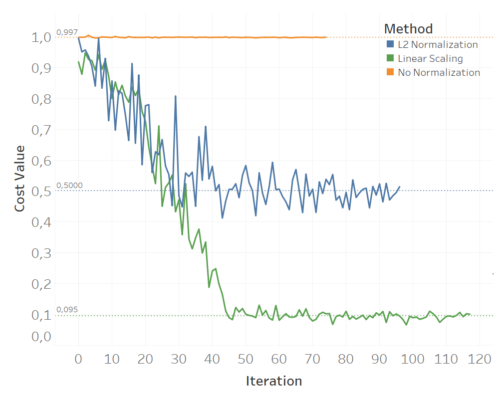
In order to prevent a particular feature from dominating the others due to its large magnitude, a data normalization technique known as linear scaling has been applied in our work, so that they all fall within the range of . It is worth highlighting that normalization significantly influences the trainability of variational ansatz, as detailed in Appendix -B.
The normalization for a feature is given by:
| (12) | ||||
where is the index of training samples.
The representation of the kernel matrix is formulated in Eq. (6). The dimension of the kernel matrix is , where is the number of samples in the training dataset. The presence of an additional row and column is a consequence of the non-zero offset . In the context of the linear equation , the kernel matrix corresponds to the matrix .
In designing hybrid quantum classical algorithms executed on current quantum hardware effectively, it is important to strategically distribute different parts of our algorithm on different computing platforms. For this reason, we use SVD prior to Pauli decomposition to reduce the number of controlled components of the kernel matrix, subsequently reducing the hard part of the calculation of the cost function. It is worthwhile to note that the Pauli decomposition in [12] is executed on a classical computer as a one-time preprocessing step. Although there exists efficient methods to simulate such decomposition on a quantum computer [22, 23], the comparison of resource overhead has not been explored in the context of employing them for variational algorithms. To that end, we aim to enhance the performance of VQLS by introducing SVD. This step is crucial towards the trainability of the variational ansatz we use and the reduction in the time for training as we will discuss in Sec. IV. Hence, we recast the problem as follows:
| (13) |
The above can be reformulated as :
| (14) |
where , . In case of the termination of the algorithm, the estimated state is related to our solution by .
Hamiltonian decomposition is a pivotal factor when it comes to variational algorithms in determining plausible effectiveness. Hence, various methods offer efficient Hamiltonian decomposition [24, 25], particulary when the Hamiltonian exhibits the sparsity. Extending the same framework to our kernel matrix, it is imperative to improve the sparsity by employing SVD for an efficient quantum subroutine.
III-C Implementation of VQLS
Building upon the basic implementation of VQLS detailed in [14], we extend its functionality to implement our VQLS-enhanced QSVM.
III-C1 Variational Ansatz
The Ansatz in the VQLS is realized by using a hardware-efficient ansatz designed for a three-qubit circuit, as introduced in [12]. The quantum circuit of this hardware-efficient ansatz, initialized with random parameters, is shown in Fig. 4.

III-C2 Quantum circuit for computing the cost function
The state is prepared with the ansatz by . The value of the cost function indicates the overlap of with the solution state . A higher cost indicates a lower overlap between current and desired solution. Therefore, it is crucial to determine an optimal set of the parameters through an optimization method on a classical computer by minimizing the cost function from Eq. (9). Details of the code to compute the cost function are explained in the pseudocode presented in Algorithm 1.
III-C3 Construction and validation of SVC
The set of optimal parameters obtained through Algorithm 1 is delivered to initialize the hardware-efficient ansatz, allowing us to estimate the vector after measurement.
The measured probabilities of each basis state in the statevector indicate the weights of , where , used in constructing the SVC. Since we obtained only the normalized statevector from the quantum subroutine, an additional machinery is required to estimate its actual magnitude. Therefore, we employ linear regression to estimate both and . Algorithm 2 shows the pseudocode, which was used for construction and validation of the SVC.
IV Results
In this section, we discuss the results of our numerical experiments, aiming to evaluate the performance of our VQLS-enhanced QSVM algorithm. In our work, we use the three qubit VQLS model and the size of the kernel matrix is .
For the VQLS subroutine, we set the termination condition for the optimization routine as follows: either the program terminates at maximum iterations (= 300) or if the cost value is the same for the last certain number of iterations. For this work,we use the IBM-Q aer simulator and the optimizer cobyla for the classical optimization routine on our local computing resource [26].
In Sec. IV-A, we show how employing SVD prior to Pauli decomposition and solving an equivalent problem gives us an edge over merely using Pauli decomposition [12], in terms of convergence to a minimum and run-time. In the rest of our analysis, we include SVD as an element in the construction of the classifiers.
In Sec. IV-B and Sec. IV-C, we use different datasets and different instances within a given dataset to derive SLEs and explore the consequent impact on the convergence of the cost function. This variation leads to SLEs with varying condition numbers, yielding insight into the behavior of VQLS in these cases. In Sec. IV-C, we also analyze the accuracy of classifiers constructed using the VQLS-enhanced QSVM, in comparison to the LS-SVM.
IV-A Impact of SVD on run-time and convergence
Since VQLS shows promise in terms of scalability to larger systems in [12], it is crucial to reduce the total number of Pauli strings in Eq. (8) for the computation of the cost function in Eq. (9) and improve its trainability. As proposed in Sec. III-B, we replace the kernel matrix with its SVD component . By solving the new system of equations given by Eq. (14), we accelerate the convergence and enhance the trainability compared to the tradional method of using Pauli decomposition for the matrix in the original problem in Eq. (13).
In our experiment, the number of Pauli strings after decomposition for and are 36 and 8, respectively. Consequently, the total number of expectation values to be computed within the sum in Eqs. (10) and (11) is reduced. For example, when the number of terms in the decomposition is given by , we need loops at most to compute the inner product in Eq. (11). In our case, this translates to 1296 () and 64 () loops for and respectively. This reduction significantly decreases the number of terms required to compute expectation values within Eqs. (10) and (11) and the run-time. The combination of SVD and Pauli decomposition reduces the system run-time to approximately one-sixteenth of what it would be used using the Pauli decomposition alone, when and in Eq. (9) are computed for our specific example. Fig. 5 illustrates the run-time for identifying an optimal set of parameters for the construction of the separating hyperplane when executed using only Pauli decomposition versus the combination of SVD and Pauli decomposition.

We also note that recasting the problem into Eq. (14) yields a lower minimum of the cost function, indicating a possibly more accurate solution. Fig. 5 also compares the final cost minima. Notably, Bravo-Prieto et al. [12, Appendix A] discuss precision of the cost function computation and its dependence on sparsity. Specifically, for a -sparse matrix, the discussion presented in [12] implies that the precision of the cost function computation is inversely proportional to . Consequently, improving sparsity by solving for instead of improves the precision of the cost function calculation. For more details on the role of sparsity in solving SLEs with quantum algorithms, we refer to [5, 25].
IV-B Influence of the condition number on the convergence of the cost function in VQLS
We study the influence of parameter on the convergence of cost function numerically, varying the values of . Numerical experiments are categorized into two parts based on the chosen dataset: toy dataset and the Iris dataset.
IV-B1 Results with toy dataset
In this analysis, we randomly choose three different instances of data. The Pauli decomposition of the matrix contains two Pauli strings, III () and YYZ (). Each instance has two different sets of coefficients. Solving each of these SLEs demonstrates a clearer understanding of the impact of on the convergence of the cost function. Fig. 6 illustrates ’s influence on convergence in three instances.

Given the substantial impact of on the convergence of the cost function shown in Fig. 6, we further investigate the relationship between the number of Pauli strings in the decomposition of several matrices with similar condition number and the convergence of the cost function. This analysis involves four instances with the kernel matrix having 10, 15, 20, and 36 Pauli strings. The condition number of all these matrices is . The convergence of the cost function is illustrated in Fig. 7.

For SLEs constructed with the toy dataset, VQLS is accurate when the kernel matrix is well conditioned. In such a situation, the number of Pauli strings in its decomposition does not play a major role.
IV-B2 Results with the Iris dataset
In this section, we present numerical results that highlight the impact of the condition number on the convergence of the cost function, when utilizing the Iris dataset to evaluate our approach without the use of SVD. We extracted one instance of training dataset, including seven samples from Setosa and Virginica, and generated five different kernel matrices using Eq. (6). The condition numbers of these kernel matrices are and , which is realized by adjusting the hyperparameter from Eq. (6). The results shown in Fig. 8 align nicely with those for the toy dataset (Fig. 6 in Sec. IV-B1).


We observe that the use of SVD in preprocessing weakens the existing correlation between the condition number of the kernel matrix and the convergence of cost function in VQLS. To evaluate our approach’s performance when utilizing the SVD, we conducted subsequent experiments using the same five kernel matrices used previously in the analysis presented in Fig. 8. The numerical results demonstrate a lower cost minimum even under a high condition number . This can be observed in Fig. 9.
The weakening of correlation between the condition number and convergence of cost function due to inclusion of SVD is advantageous. This results in a better convergence at higher condition numbers and a significant enhancement in the trainability of variational ansatz.
IV-C Performance evaluation of SVC built with VQLS-enhanced QSVM

In this analysis, we consider ten random instances of training sets from the Iris dataset. Four of them have , three fall within and three have .
The classification hyperplanes for these ten instances are constructed using the VQLS-enhanced QSVM detailed in Sec. III. For accuracy validation, we compare the performances of QSVM-based and LS-SVM-based classifiers. The influence of different condition numbers of the kernel matrix, which are manipulated through , is evident on the classifier accuracy as seen in Fig. 10. The final cost values are also plotted for these matrices alongside the accuracy. Furthermore, Table. IV in Appendix -D shows the evaluation of classification performance employing a range of metrics.
Furthermore, we repeated each of our numerical experiments five times to examine the stability. Table. I displays the experimental results for one instance. Based on the table, it is evident that the majority of the outcomes yields similar classification accuracy. Results of three more experiments for additional instances are reported in Appendix -C. It is important to note that having a lower cost value does not inherently guarantee higher classification accuracy. This is due to the fact that a lower cost value does not guarantee an accurate solution in the case of VQLS [12]. Hence, it is important to include a verification step to validate the solution.
| No. | No. of incorrect classification | accuracy of our SVC | accuracy of classical SVC | |
| 1 | 1 | |||
| 2 | 1 | |||
| 4.8 | 3 | 1 | ||
| 4 | 1 | |||
| 5 | 41 | |||
| 1 | 1 | |||
| 2 | 1 | |||
| 287 | 3 | 1 | ||
| 4 | 1 | |||
| 5 | 46 | |||
| 1 | 50 | |||
| 2 | 50 | |||
| 4594 | 3 | 50 | ||
| 4 | 50 | |||
| 5 | 48 |
V Conclusion and Outlook
This work aims to identify an optimal set of parameters for constructing a classifier on a quantum computer. We then use this classifier to complete the classification tasks in supervised learning. This objective is realized by utilizing our proposed hybrid quantum-classical algorithm on NISQ devices, named as the VQLS-enhanced QSVM. Additionally, we benchmarked this approach by examining the SVC with real-world data, the Iris dataset.
The VQLS-enhanced QSVM is capable of robustly identifying a separating hyperplane that highly accurately classify samples in the test data. We note that SVD is crucial for minimizing the number of controlled unitaries applied during a Hadamard test. Hence, we applied SVD on the kernel matrix in our numerical experiments. It significantly reduces the number of expectation values computed in one iteration for a faster and more accurate result. Furthermore, appropriately selecting the hyper parameter in Eq. (6), utilized for the design of the kernel matrix, crucially influences both the trainability of variational ansatze and the classification accuracy. The classifiers constructed using our approach exhibits a strong performance for problems with small condition number of the kernel matrix .
This work can be further explored by employing noise models and executing numerical experiments on real quantum hardware. It is also worthwhile to investigate the scalability of the VQLS-based QSVM with increasing problem size.
Acknowledgment
We thank Katja Schladitz and Alexander Geng for helpful conversations regarding the manuscript. This work was funded by the Federal Ministry for Economic Affairs and Climate Action (German: Bundesministerium für Wirtschaft und Klimaschutz) under the project EniQmA with funding number 01MQ22007A.
References
- [1] N Vladimir and Vlamimir Vapnik “Statistical learning theory” In Xu JH and Zhang XG. translation. Beijing: Publishing House of Electronics Industry, 2004, 1998
- [2] Kok Chua “Efficient computations for large least square support vector machine classifiers” In Pattern Recognition Letters 24.1, 2003, pp. 75–80
- [3] Johan Suykens and Joos Vandewalle “Least squares support vector machine classifiers” In Neural processing letters 9 Springer, 1999, pp. 293–300
- [4] Patrick Rebentrost, Masoud Mohseni and Seth Lloyd “Quantum support vector machine for big data classification” In Physical review letters 113.13 APS, 2014, pp. 130503
- [5] Aram Harrow, Avinatan Hassidim and Seth Lloyd “Quantum algorithm for linear systems of equations” In Physical review letters 103.15 APS, 2009, pp. 150502
- [6] Abhinav Kandala et al. “Hardware-efficient variational quantum eigensolver for small molecules and quantum magnets” In Nature 549.7671 Nature Publishing Group UK London, 2017, pp. 242–246
- [7] Jacob Biamonte et al. “Quantum machine learning” In Nature 549.7671 Nature Publishing Group UK London, 2017, pp. 195–202
- [8] Vojtěch Havlíček et al. “Supervised learning with quantum-enhanced feature spaces” In Nature 567.7747 Nature Publishing Group UK London, 2019, pp. 209–212
- [9] Hong Li et al. “Quantum support vector machine based on gradient descent” In International Journal of Theoretical Physics 61.3 Springer, 2022, pp. 92
- [10] Rui Zhang et al. “Quantum support vector machine based on regularized Newton method” In Neural Networks 151 Elsevier, 2022, pp. 376–384
- [11] Zhaokai Li, Xiaomei Liu, Nanyang Xu and Jiangfeng Du “Experimental realization of a quantum support vector machine” In Physical review letters 114.14 APS, 2015, pp. 140504
- [12] Carlos Bravo-Prieto et al. “Variational quantum linear solver” In arXiv preprint arXiv:1909.05820, 2019
- [13] R.. Fisher “Iris” UCI Machine Learning Repository, 1988 DOI: 10.24432/C56C76
- [14] Qiskit contributors “Qiskit: An Open-source Framework for Quantum Computing”, 2023 DOI: 10.5281/zenodo.2573505
- [15] Vivek Shende, Stephen Bullock and Igor Markov “Synthesis of quantum logic circuits” In Proceedings of the 2005 Asia and South Pacific Design Automation Conference, 2005, pp. 272–275
- [16] Samson Wang et al. “Noise-induced barren plateaus in variational quantum algorithms” In Nature communications 12.1 Nature Publishing Group UK London, 2021, pp. 6961
- [17] Marco Cerezo et al. “Cost function dependent barren plateaus in shallow parametrized quantum circuits” In Nature communications 12.1 Nature Publishing Group UK London, 2021, pp. 1791
- [18] Jules Tilly et al. “The variational quantum eigensolver: a review of methods and best practices” In Physics Reports 986 Elsevier, 2022, pp. 1–128
- [19] Michael Powell “A direct search optimization method that models the objective and constraint functions by linear interpolation” Springer, 1994
- [20] Giacomo Nannicini “Performance of hybrid quantum-classical variational heuristics for combinatorial optimization” In Physical Review E 99.1 APS, 2019, pp. 013304
- [21] Aidan Pellow-Jarman, Ilya Sinayskiy, Anban Pillay and Francesco Petruccione “A comparison of various classical optimizers for a variational quantum linear solver” In Quantum Information Processing 20.6 Springer, 2021, pp. 202
- [22] Mohsen Heidari and Wojciech Szpankowski “Learning k-qubit Quantum Operators via Pauli Decomposition” In International Conference on Artificial Intelligence and Statistics, 2023, pp. 490–504 PMLR
- [23] Ashley Montanaro and Tobias Osborne “Quantum boolean functions” In arXiv preprint arXiv:0810.2435, 2019
- [24] Dominic Berry, Graeme Ahokas, Richard Cleve and Barry Sanders “Efficient quantum algorithms for simulating sparse Hamiltonians” In Communications in Mathematical Physics 270 Springer, 2007, pp. 359–371
- [25] Andrew Childs, Robin Kothari and Rolando Somma “Quantum algorithm for systems of linear equations with exponentially improved dependence on precision” In SIAM Journal on Computing 46.6 SIAM, 2017, pp. 1920–1950
- [26] We use Intel-2670., Running at system specifications of 2.60 Hz and 64 GB RAM. This system was used for all numerical experiments.
-A An instance of the training dataset
In this section, in Table. II we have an overview of one instance of dataset used for training.
| No. | Sepal Length | Sepal Width | Petal length | Petal Width | Sepal |
| 1 | 5.1 | 3.5 | 1.4 | 0.2 | Setosa |
| 2 | 4.9 | 3.0 | 1.4 | 0.2 | Setosa |
| 3 | 4.7 | 3.2 | 1.3 | 0.2 | Setosa |
| 4 | 5.0 | 3.6 | 1.4 | 0.2 | Setosa |
| 5 | 6.7 | 3.0 | 5.2 | 2.3 | Virginica |
| 6 | 6.3 | 2.5 | 5.0 | 1.9 | Virginica |
| 7 | 5.9 | 3.0 | 5.1 | 1.8 | Virginica |
-B Influence of the data normalization technique on the cost function convergence
Data normalization plays a key role in data preprocessing, particularly in machine learning and data analysis. It encompasses the transformation of data into a standardized format or scale, thereby enhancing its suitability for subsequent analysis or model training. The significance of data normalization is introduced by our cost function convergence analysis in Fig. 11.
-C Numerical results for evaluating the stability with additional instances of the kernel matrix
The data in Table. III indicates that most of the classification results are similarly precise.
| Instance 1 | ||||
| No. | No. of incorrect classification | accuracy of our SVC | accuracy of classical SVC | |
| 1 | 1 | |||
| 2 | 3 | |||
| 17 | 3 | 1 | ||
| 4 | 1 | |||
| 5 | 37 | |||
| 1 | 1 | |||
| 2 | 49 | |||
| 30 | 3 | 1 | ||
| 4 | 1 | |||
| 5 | 5 | |||
| 1 | 1 | |||
| 2 | 3 | |||
| 319 | 3 | 1 | ||
| 4 | 14 | |||
| 5 | 48 | |||
| Instance 2 | ||||
| No. | No. of incorrect classification | accuracy of our SVC | accuracy of classical SVC | |
| 1 | 1 | |||
| 2 | 7 | |||
| 11 | 3 | 1 | ||
| 4 | 44 | |||
| 5 | 41 | |||
| 1 | 14 | |||
| 2 | 50 | |||
| 35 | 3 | 1 | ||
| 4 | 1 | |||
| 5 | 2 | |||
| 1 | 2 | |||
| 2 | 31 | |||
| 14742 | 3 | 37 | ||
| 4 | 1 | |||
| 5 | 49 | |||
| Instance 3 | ||||
| No. | No. of incorrect classification | accuracy of our SVC | accuracy of classical SVC | |
| 1 | 50 | |||
| 2 | 50 | |||
| 8 | 3 | 46 | ||
| 4 | 49 | |||
| 5 | 49 | |||
| 1 | 1 | |||
| 2 | 50 | |||
| 21 | 3 | 48 | ||
| 4 | 1 | |||
| 5 | 46 | |||
| 1 | 50 | |||
| 2 | 50 | |||
| 222 | 3 | 1 | ||
| 4 | 50 | |||
| 5 | 50 | |||
-D Numerical results for classification accuracy with additional instances of the kernel matrix
Table. IV summarizes the main classification metrics for two instances from the Iris dataset.
| Matrix | |||||
| Class | Precision | Recall | F1-score | Support | |
| 5.5 | Virginica | 0.98 | 1.00 | 0.99 | 50 |
| Setosa | 1.00 | 0.98 | 0.99 | 50 | |
| 13 | Virginica | 0.91 | 1.00 | 0.95 | 50 |
| Setosa | 1.00 | 0.90 | 0.95 | 50 | |
| 17 | Virginica | 0.91 | 1.00 | 0.95 | 50 |
| Setosa | 1.00 | 0.90 | 0.95 | 50 | |
| 25 | Virginica | 0.74 | 1.00 | 0.85 | 50 |
| Setosa | 1.00 | 0.64 | 0.78 | 50 | |
| 287 | Virginica | 0.00 | 0.00 | 0.00 | 50 |
| Setosa | 0.50 | 1.00 | 0.67 | 50 | |
| 5696 | Virginica | 0.00 | 0.00 | 0.00 | 50 |
| Setosa | 0.50 | 1.00 | 0.67 | 50 | |
| Matrix | |||||
| Class | Precision | Recall | F1 - score | Support | |
| 4.8 | Virginica | 0.98 | 1.00 | 0.99 | 50 |
| Setosa | 1.00 | 0.98 | 0.99 | 50 | |
| 10 | Virginica | 0.98 | 1.00 | 0.99 | 50 |
| Setosa | 1.00 | 0.98 | 0.99 | 50 | |
| 13 | Virginica | 0.88 | 1.00 | 0.93 | 50 |
| Setosa | 1.00 | 0.86 | 0.92 | 50 | |
| 19 | Virginica | 0.98 | 1.00 | 0.99 | 50 |
| Setosa | 1.00 | 0.98 | 0.99 | 50 | |
| 144 | Virginica | 0.52 | 1.00 | 0.68 | 50 |
| Setosa | 1.00 | 0.08 | 0.15 | 50 | |
| 4594 | Virginica | 0.00 | 0.00 | 0.00 | 50 |
| Setosa | 0.50 | 1.00 | 0.67 | 50 | |
we present the classification accuracy for the repetitions of a specific instance in Table. V. This also serves as a stability analysis for the program.
| Instance | No. of incorrect classification | accuracy of our SVC | accuracy of classical SVC | ||
| 5 | 1 | ||||
| 11 | 1 | ||||
| 1 | 19 | 7 | |||
| 144 | 46 | ||||
| 4594 | 50 | ||||
| 6 | 2 | ||||
| 13 | 5 | ||||
| 3 | 25 | 5 | |||
| 287 | 18 | ||||
| 5696 | 1 | ||||
| 18 | 1 | ||||
| 30 | 46 | ||||
| 4 | 319 | 3 | |||
| 635 | 47 | ||||
| 6961 | 1 | ||||
| 5 | 1 | ||||
| 11 | 6 | ||||
| 5 | 21 | 50 | |||
| 138 | 1 | ||||
| 5230 | 1 | ||||
| 18 | 1 | ||||
| 30 | 46 | ||||
| 6 | 319 | 3 | |||
| 635 | 47 | ||||
| 6961 | 1 | ||||
| 21 | 50 | ||||
| 50 | 18 | ||||
| 7 | 76 | 37 | |||
| 178 | 1 | ||||
| 8302 | 50 | ||||
| 22 | 48 | ||||
| 30 | 49 | ||||
| 8 | 102 | 45 | |||
| 156 | 1 | ||||
| 7880 | 50 | ||||
| 26 | 50 | ||||
| 34 | 1 | ||||
| 9 | 47 | 1 | |||
| 544 | 1 | ||||
| 7528 | 1 | ||||
| 25 | 50 | ||||
| 34 | 49 | ||||
| 10 | 83 | 50 | |||
| 178 | 50 | ||||
| 8936 | 50 | ||||
| 34 | 49 | ||||
| 39 | 3 | ||||
| 11 | 65 | 50 | |||
| 370 | 1 | ||||
| 8887 | 13 |
