On dynamics of the Chebyshev’s method for quartic polynomials
Abstract
Let be a normalized (monic and centered) quartic polynomial with non-trivial symmetry groups. It is already known that if is unicritical, with only two distinct roots with the same multiplicity or having a root at the origin then the Julia set of its Chebyshev’s method is connected and symmetry groups of and coincide [Nayak, T., and Pal, S., Symmetry and dynamics of Chebyshev’s method, [5]]. Every other quartic polynomial is shown to be of the form where . Some dynamical aspects of the Chebyshev’s method of are investigated in this article for all real . It is proved that all the extraneous fixed points of are repelling which gives that there is no invariant Siegel disk for . It is also shown that there is no Herman ring in the Fatou set of . For positive , it is proved that at least two immediate basins of corresponding to the roots of are unbounded and simply connected. For negative , it is however proved that all the four immediate basins of corresponding to the roots of are unbounded and those corresponding to are simply connected.
Keyword:
Quartic polynomials; Fatou and Julia sets; Symmetry; Chebyshev’s method.
AMS Subject Classification: 37F10, 65H05
1 Introduction
A root-finding method is a function from the space of all polynomials that assigns a rational map to a polynomial such that each root of is an attracting fixed point of , i.e., if is a root of then and . Though there are several such methods appearing in the literature, the family of König’s methods [2] and Chebyshev-Halley methods [3] seem to be comparatively well-studied among them. The Newton method is the first member of the König’s methods and its order of convergence (i.e., the local degree of at each of the simple roots of ) is two. Further, it has no finite extraneous fixed point, i.e., each finite fixed point of is a root of . Note that the sequence of forward iterates of every root-finding method converges to a root of a polynomial in a suitably small neighborhood of the root. The non-existence of finite extraneous fixed points for the Newton method have been found to be crucial in the study of its global dynamics (i.e., not only in a neighborhood of the roots of the polynomial but in ) of the Newton method. For example, this is precisely the reason why the Julia set (it is the set of all points in at which the sequence of iterates is not normal [1]) of the Newton method applied to a polynomial is connected [9]. These are possibly some reasons for which this method has drawn a good amount of attention of researchers. However there are root-finding methods whose order of convergence is three and which has finite extraneous fixed points. One such, namely the Chebyshev’s method is the subject of this article.
For a polynomial , its Chebyshev’s method is given by
where
The Fatou set of a rational map , denoted by is the set of all points in in a neighborhood of which is normal. Its complement in is known as the Julia set of and is denoted by . A maximally connected open subset of the Fatou set, called a Fatou component is said to be periodic if . It is well-known that for every Fatou component of a rational map , there is a such that is periodic. A periodic Fatou component can be an attracting domain, a parabolic domain, a Siegel disk or a Herman ring. Other properties of these Fatou component can be found in [1]. We are concerned with the dynamics (the Fatou and the Julia sets) of the Chebyshev’s method applied to polynomials. The nature of extraneous fixed points and some other dynamical aspects of Chebyshev’s method applied to quadratic and cubic polynomial have been studied in [7]. Existence of superattracting cycles for Chebyshev’s method applied to cubic polynomial are investigated in [8]. The first systematic study of the dynamics of Chebyshev’s method applied to cubic polynomials can be found in [4]. The family of Chebyshev’s method applied to cubic polynomials is parametrized in terms of the multiplier of an extraneous fixed point and its dynamics is determined for parameters in . A discussion of the Chebyshev’s method applied to some quartic polynomials appeared in [5] which mainly deals with the relation between the group of Euclidean isometries preserving the Julia set of a polynomial and its Chebyshev’s method, whenever the earlier is non-trivial. It is shown that both these groups are isomorphic for all centered cubic and quartic polynomials with non-trivial symmetry groups.
This article deals with the quartic polynomials. First, we parametrize the family of maps arising as the Chebyshev’s method of quartic polynomials.
A root-finding method is said to satisfy the Scaling theorem (see [4]) if for every affine map and every non-zero constant , where . A quartic polynomial is of the form where . It is well-known that every polynomial can be transformed to a monic and centered (called normalized) polynomial by post-composing an affine map and then multiplying by a suitable non-zero constant . Indeed, by taking to be the reciprocal of the leading coefficient of and where is the centroid of (see page 205, [1]), it can be seen that is normalized. As the Chebyshev’s method satisfies the Scaling theorem (See Theorem 2.2, [4]), . Therefore, without loss of generality we assume that is normalized, i.e., and . Then
| (1) |
Though the ongoing discussion is on polynomials, we define the symmetry group of the Julia set of a rational map . It is denoted by and is defined as . A normalized polynomial can be written as
| (2) |
where is a monic polynomial, and are maximal. We call it normal form of and it is unique. Then by Theorem 9.5.4, [1],
Note that if and only if is trivial.
If then . Further, if then is a monomial, whose Chebyshev’s method is a linear map and this case is not of interest. As seen in the following is non-trivial in all other situations.
- Case 1:
If then and .
- Case 2:
If then and .
- Case 3:
If then and .
For the quartic polynomial of the form given in Equation 1, let . If both and are non-zero then is in its normal form with and . If and then in its normal form is , and and . Similarly, if and then is in its normal form with and . On the other hand if both are zero then and . This is the only case for where is non-trivial.
- Case 4:
, and in this case.
In this article, we attempt to understand the dynamics of for all quartic with non-trivial . The non-identity elements of are used to understand the dynamics of . This approach of determining the dynamics by the symmetries does not work when is trivial. This is a reason why this case needs to be dealt with differently, which we postpone for our future work.
The polynomials in Case are unicritical. Those in Cases and have one of their roots at the origin (the centroid of ) and have non-trivial symmetry. The dynamics of the Chebyshev’s method applied to these polynomials and those in Case having exactly two distinct roots follows from Theorem 1.3, [5]. In all these cases, the Julia set is found to be connected and . Whether, these are true for the rest of the cases is not known.
The polynomials given in Case 3 can not have exactly three distinct roots because zero is not a root and the roots appear in pairs symmetric about the origin. Note that, in Case , can be expressed as , where . The Chebyshev’s method of is conjugate to by Scaling theorem. Therefore, assume without loss of generality that where . If then is of the form as given in Case ; if then has exactly two roots with the same multiplicity, which is already dealt with in Theorem 1.3 (1) of [5]. Hence it is sufficient to consider where . Further, if then consider the polynomial , whose Chebyshev’s method is conjugate to by the Scaling theorem.
Therefore, it is enough to consider
| (3) |
where . We denote the Chebyshev’s method of by . This paper takes up the case when is real. All extraneous fixed points of are shown to be repelling. As a consequence, it follows that there is no invariant Siegel disk for . This is because every such Siegel disk requires an indifferent fixed point whereas all fixed points are found to be either attracting (when these are the roots of ) or repelling (where these are extraneous). It is proved that every periodic Fatou component on which a multiply connected Fatou component lands is an attracting or parabolic domain corresponding to a real periodic point. Here, we say a Fatou component lands on a Fatou component if there is a such that . In particular this means that there is no Herman ring in the Fatou set of . It is also found that the Julia set of is connected if and only if the Julia component containing a non-zero pole is unbounded.
For we have proved that the immediate basins of and are unbounded and at least two immediate basins (out of four corresponding to the four roots of ) are simply connected. For , all the immediate basins corresponding to the four roots of are found to be unbounded and those corresponding to the purely imaginary roots are shown to be simply connected. Under the assumption that the Fatou set is the union of the basins of attraction of the fixed points corresponding to the roots of , it is shown that for all positive . For negative this is proved with an additional assumption that the largest positive extraneous fixed point and the purely imaginary extraneous fixed points are with the same absolute value.
Section 1 describes some useful properties of . Results on fixed points and dynamics of are stated and proved in the first part of Section 2. Then in the two subsections of Section 2, the main results are proved.
By conjugacy, we mean conformal conjugacy throughout this article.
2 Basic properties of
Now, we enumerate some basic properties of .
Lemma 2.1.
- 1.
(Degree) The map is an odd rational map of degree ten.
- 2.
(Critical points) The map has eighteen critical points, counting with multiplicities. The multiple critical points are the four (simple) roots of and three poles of . Each of these has multiplicity two as a critical point of . The other four critical points are simple. If is real then these four critical points are neither real nor purely imaginary and the poles are all real.
- 3.
(Fixed points) The roots of are the superattracting fixed points of . The point at infinity is a repelling fixed point of with multiplier . The extraneous fixed points are the solutions of .
Proof.
- 1.
It follows from Equation 5 that is an odd rational map with degree ten.
- 2.
By Theorem 2.7.1. [1], has eighteen critical points counting with multiplicity. Recall that the multiplicity of a critical point is one less than the local degree of the function at that point. The derivate of is
(6) The critical points of are , , each of multiplicity (these are the roots of ), with multiplicity each (these are the poles of ) and the solutions of
(7) The above equation has four distinct roots, namely the solutions of and each is a simple critical point of .
That simple critical points are neither real nor purely imaginary and non-zero poles are real whenever is obvious.
- 3.
As the roots of are fixed points as well as critical points of , their multiplier is zero. In other words, these are superattracting fixed points of . It is evident from Equation 5 that the degree of the numerator is bigger than that of the denominator of giving that is a fixed point of . Its multiplier is (see page no. 41 [1] for the formula). Thus is a repelling fixed point of .
∎
Remark 2.1.
- 1.
(Free critical points) The critical points and are superattracting fixed points of . The poles and are also critical points and are mapped to which is a repelling fixed point of . Hence the poles are in the Julia set.
In order to determine the existence of Fatou components different from the basins of superattracting fixed points, the forward orbits of the four simple critical points of need to be followed. These are and where and are principal square roots of and respectively. Following the general practice, we call these as free critical points.
- 2.
If is a free critical point then
For
Further, if is real then
where and . Since ,
Note that if then and . But and can be shown not to have any common root. Hence the critical values corresponding to the free critical points are non-zero whenever is real.
3 Dynamics of for real parameter
In view of Equation 3, for every real , is conjugate to for some . The study of dynamics of is undertaken in this section. We start with an almost obvious but useful observation. We say a Fatou component lands on a Fatou component if there is a such that . Note that every Fatou component lands on each of its iterated forward image and in particular, periodic Fatou components land on themselves. By Sullivan’s No Wandering theorem, every Fatou component of a rational map lands on a periodic Fatou component.
Lemma 3.1.
For every non-zero real , preserves the real as well as the imaginary axis. Further, the following are true about the Fatou set of .
- 1.
If a Fatou component intersects either the real axis or the imaginary axis then it does not land on any rotation domain (Siegel disk or Herman ring).
- 2.
No Fatou component intersects both the real and the imaginary axis.
- 3.
The Julia component containing the origin is unbounded.
Proof.
Since all the coefficients of the denominator and numerator of are real, . Now for every ,
| (9) |
where and are defined in Equation 5. This shows that the imaginary axis is preserved by .
- 1.
We prove this assuming that a Fatou component intersects the real axis. The proof in the other case, when the Fatou component intersects the imaginary axis, is exactly the same. Let a Fatou component intersect the real axis and let . If lands on a rotation domain with period , then for some . Now for all where . Since is conformally conjugate to an irrational rotation (for some irrational number ) on a disk or on an annulus about the origin, the set is dense in a Jordan curve contained in . Since is real for all , this Jordan curve can only be . But is not in the Fatou set leading to a contradiction.
- 2.
If a Fatou component of intersects both the real and the imaginary axis then the periodic Fatou component on which it lands intersects both the axes and hence can not be a rotation domain by (1) of this lemma. Therefore, it must be an attracting or parabolic domain. The corresponding periodic points are in the intersection of both the axes because both the axes are invariant under . In other words, the periodic point can only be either or . Since and is a fixed point, the periodic point must be . But is a repelling fixed point leading to a contradiction.
- 3.
If the Julia component containing the origin is bounded then a Jordan curve can be found in the Fatou set surrounding the origin, i.e., the bounded component of the complement of the Jordan curve contains the origin. The Fatou component containing this Jordan curve has to intersect both the real and the imaginary axes, which is not possible by (2) of this lemma. Therefore, the Julia component containing the origin is unbounded.
∎
There are some important consequences. We say a Fatou component surrounds a point if the point is in a bounded component of its complement.
Theorem 3.2.
If is a multiply connected Fatou component of then there is an such that is a Fatou component surrounding a non-zero pole. If is a periodic Fatou component on which lands then is an attracting or parabolic domain corresponding to a real periodic point. In particular, there is no Herman ring for .
Proof.
Consider a Jordan curve such that each of its complementary component intersects the Julia set. Since the Julia set is the closure of the backward orbit of any point in it (see Theorem 4.2.7 (ii), [1]) and all the poles are in the Julia set of , there is an such that surrounds a pole of . Indeed, can be taken as the smallest natural number such that is analytic in the bounded component of the complement of and the preceding statement follows from the Open Mapping Theorem. The curve can not surround the pole at the origin by Lemma 3.1(3) and therefore it surrounds a non-zero pole. The Fatou component containing clearly surrounds the non-zero pole of .
If is a periodic Fatou component on which lands then intersects the real line because the real line invariant under and intersects the real line. Since can not be a rotation domain, it is either an attracting domain or a parabolic domain. Again the invariance of the real line under gives that the periodic point corresponding to must be real.
Since Herman rings are multiply connected, it must land on an attracting or parabolic domain which is absurd. Therefore does not have any Herman ring. ∎
Note that there are two non-zero poles and the Julia component containing one is bounded if and only if that containing the other is bounded. This is because is an odd function giving that if and only if . The boundedness of such Julia components determines the connectedness of the whole Julia set.
Corollary 3.2.1.
The Julia set of is connected if and only if the Julia component containing a non-zero pole is unbounded.
Proof.
If the Julia set of is connected then there is only a single Julia component. Since and the non-zero poles are in the Julia set, the Julia component containing a non-zero pole is unbounded. Conversely, if the Julia set is not connected then there is a multiply connected Fatou component, say . By Theorem 3.2, there is an such that surrounds a non-zero pole. In particular, the Julia component containing this non-zero pole is bounded. In other words, if the Julia component containing a non-zero pole is unbounded then the Julia set is connected. ∎
For , all the roots of are real where as for , has two real and two purely imaginary roots. These two cases need to be treated differently. Before we consider them separately, two useful lemmas are presented.
Lemma 3.3 (Symmetry about the coordinate axes).
The map preserves the Fatou and the Julia sets of for all real non-zero . In particular, if a Fatou component contains a real (or a purely imaginary) number then it is symmetric about the real axis (or the imaginary axis respectively).
Proof.
Since is odd and all the coefficients of its denominator as well as numerator are real, . Therefore, if then for all and all . This gives that and . ∎
If is an extraneous fixed point of then its multiplier is given by the formula (see [4]), which is nothing but
| (10) |
Lemma 3.4.
All the real extraneous fixed points of are repelling for every non-zero .
Proof.
For every if denotes the positive square root of then can be rewritten as
In order to determine the multipliers of the real extraneous fixed points, we need to analyse the function
on the real line. It suffices to do it in as the function is even.
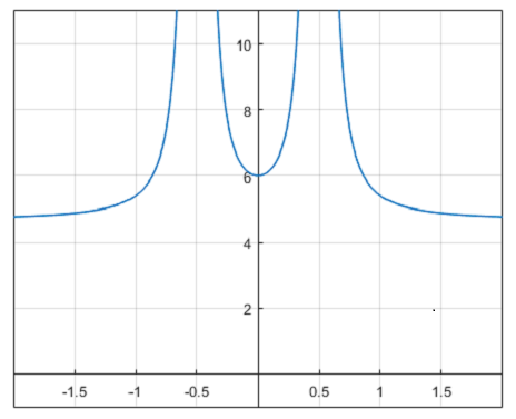
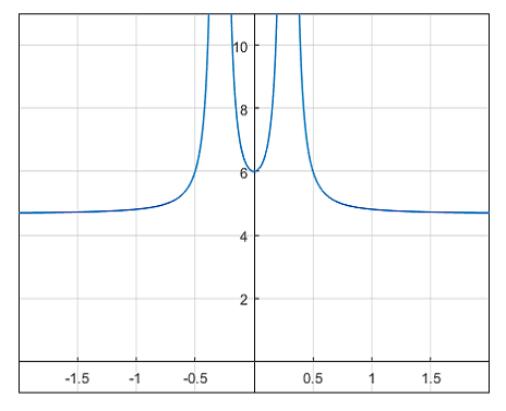
The function for all and therefore is increasing in this interval. Consequently, for all . Similarly, for all . Since , is a strictly decreasing function in with minimum value . Consequently for all real . Thus the multiplier of every real extraneous fixed point of is at least . Hence every real extraneous fixed point of is repelling. The graphs of are given in Figure 1. ∎
3.1 Positive parameter
First, we determine the location of extraneous fixed points. Recall that there are six extraneous fixed point of and these are the solutions of where is as given in Lemma 2.1(3).
Lemma 3.5.
All the extraneous fixed points of are in and hence are repelling.
Proof.
In view of Lemma!3.4, it is enough to show that all the extraneous fixed points of are in . Let and
(see Lemma 2.1(3)). Then , , and . Therefore, has a root in each of the intervals , and , and the square roots of these roots are precisely the extraneous fixed points of . If are the positive extraneous fixed points in decreasing order then
and the other three extraneous fixed points satisfy
Thus all the extraneous fixed points of for are in . ∎
The graph of , is described in Figure 2(a). Green dots represent the extraneous fixed points, blue dots along with are the superattracting fixed points of corresponding to the roots of , whereas the poles are indicated by the red dots.
From Equation (2), for , we have
As is not zero for any real and is positive at (see Equation 7), for all real . Therefore, is increasing in . Further,
| (11) |
where are as mentioned in Lemma 3.5. Recall that has four superattracting fixed points, namely and these are all real. Let be their respective immediate basins of attractions.
Theorem 3.6.
The immediate basins and contain and respectively. In particular, these are unbounded and their respective boundaries contain a pole.
Proof.
It follows from Equation 11 that for every , . Since is strictly increasing, for every . This implies that converges to for every , i.e., . Now maps onto itself and by Equation 11. Since is strictly increasing in this interval, for all . In other words, and in particular is unbounded.
Since is invariant and unbounded, it follows from Lemma 4.3 [4] that its boundary contains a pole.


As is odd, and is also unbounded. Further, its boundary contains a pole. ∎
Remark 3.1.
- 1.
- 2.
Since is strictly increasing in and , the left hand limit of at is . Hence has a unique root in . Now is contained in and therefore does not contain any root of (as roots are in the Julia set). Repeating the same argument for in , it is found that has a unique root between and . Since is odd, it has two positive roots, one in and the other in .
Recall from Equation 9 that where
Here are as given in Equation 5. Further, is a real-valued function defined on the real axis and , where . Note that for all real non-zero ,
| (12) |
It is enough to study the function on the real line for understanding on the imaginary axis.
First we look at the possible zeros of on the imaginary axis.
Lemma 3.7.
The function has exactly two purely imaginary roots.
Proof.
Consider . Then and . Since , there is an such that . As , has a root in . This root is unique as is strictly increasing by Equation 12. It follows from the discussion preceding this lemma that has two purely imaginary roots. ∎
Here is a remark.
Remark 3.2.
Note that is a critical point of , and is an increasing function on the negative real axis. As has no fixed point on the imaginary axis, the same is true for . Since , for all . As is an odd function, for all (see Figure 2(b)).
Though the imaginary axis does not contain any fixed point of , the existence of periodic or pre-periodic points in the imaginary axis can not be ruled out.
Observation 1.
The imaginary axis contains two-periodic points of and those are repelling.
Proof.
Let be the positive root of and . Then and . In fact, maps bijectively onto . The branch of such that is a contraction. By the Contraction Mapping Principle, has a fixed point in . As does not have any fixed point on the real line by Remark 3.2, this fixed point of is a two periodic point of . Further, this is attracting for and hence repelling for . Since , has a repelling -periodic point on the positive imaginary axis. ∎
Remark 3.3.
Using similar arguments, it can be seen that has a two periodic point in . Indeed, this is in the same cycle of the two periodic point mentioned in the above lemma.
As is real for every real , is a real number for every purely imaginary . Therefore, the periodic points of lying on the imaginary axis can not be irrationally indifferent. Thus, these are attracting, rationally indifferent or repelling. If these are repelling then we have an important consequence.
Lemma 3.8.
If all the periodic points of lying on the imaginary axis are repelling then the imaginary axis is in the Julia set of .
Proof.
Suppose on the contrary that there is a Fatou component intersecting the imaginary axis. Let be the periodic Fatou component on which lands. Then intersects the imaginary axis and by Lemma 3.1, can not be a rotation domain. The other possibility that is an attracting domain or a parabolic domain would imply that the corresponding attracting or parabolic periodic point must be purely imaginary, which is contrary to the hypothesis. This completes the proof. ∎
Though each multiply connected Fatou component is restricted in the sense that it lands on a Fatou component intersecting the real axis, their existence can not be completely ruled out. We are able to show that not all immediate basins of superattracting fixed points of corresponding to the roots of are multiply connected.
Theorem 3.9.
At least two immediate basins of attraction corresponding to the roots of are simply connected.
Proof.
If none of the immediate basins contain any free critical point then these are simply connected by Theorem 3.9 [6].
If there is a free critical point say in an immediate basin of attraction of then . This is because each Fatou component containing a real number is symmetric about the real axis by Lemma 3.3. Further, it follows from the same lemma that . Therefore, the other two immediate basins of superattracting fixed points contain no critical points other than the respective roots of . Hence these two immediate basins of attraction (corresponding to the roots of ) are simply connected by Theorem 3.9 [6]. ∎
Here is a remark.
Remark 3.4.
We have the following result about the symmetry group of the Julia set of .
Theorem 3.10.
If the Fatou set of consists only of the basins of attraction of the superattracting fixed points of then .
Proof.
It is known that and every element of is a rotation about the origin, the centroid of (Theorem 1.1. [5]). It is shown in Theorem 3.6 that the immediate basins are unbounded. As is a repelling fixed point, by Lemma 3.2. [5], every Fatou component landing on these immediate basins is bounded. If are bounded then every Fatou component landing on these will be bounded as is a fixed point. On the other hand, if are unbounded then Lemma 3.2. [5] gives that every Fatou component landing on is bounded. Hence the Fatou set of contains at most four unbounded components.
Let . Then can not be equal to or and therefore or . Thus is either the identity or . Since is the only non-identity element of , we have . Thus and hence . ∎
Remark 3.5.
- 1.
If and the Fatou set of consists of only the basins of the fixed points of corresponding to the roots of (all of these are real) then there is no Fatou component intersecting the imaginary axis. This is because the imaginary axis is invariant and no Fatou component can intersect both the axes. Therefore, the imaginary axis is in the Julia set of where and consists of only the basins of the fixed points of corresponding to the roots of .
- 2.
It is not known whether the non-zero poles are on the boundary of or not.
- 3.
For it is believed (but yet not proved) that the immediate basins are unbounded. This is supported by Figure 3(a), which is generated using MatLab.


Figure 3(a) illustrates the Fatou and the Julia sets of . The largest regions in deep blue, blue, yellow and deep yellow represent the immediate basins of attractions of and respectively. All the smaller regions in deep blue belong to the basin (but not the immediate basin) of . Similar is the case of smaller regions in other three colours. The Julia set is the complement of the union of these four basins.
3.2 Negative parameters
We are to deal with for . Let where so that
for . Then the Chebyshev’s method of of , denoted by , is defined as
| (13) |
where , , and . The critical points of are , each with multiplicity two and the solutions of (see Equation 7) which are all simple. If is such a solution then .
We prove as in positive parameter case that all extraneous fixed points are repelling.
Lemma 3.11.
All the extraneous fixed points of for are repelling.
Proof.
The extraneous fixed points are the solutions of Equation 8. Let and . Then , , and . Therefore has a root in each of the intervals and and the square roots of these roots are precisely the extraneous fixed points of . There are four real and two purely imaginary extraneous fixed points. If are the positive extraneous fixed points in decreasing order then
It follows from Lemma 3.4 that these four (real) extraneous fixed points are repelling.
If are purely imaginary extraneous fixed points such that then is a square root of the negative root of (lying in ) and therefore,
If is an extraneous fixed point of then its multiplier is given by where . Let be defined by
Then
| (14) |
Since is even, it is enough to analyse it in . Since , is a repelling fixed point of if and only if . We are going to establish this by showing that for all . This is so because . There are two cases depending on whether or .
If then and for all . Therefore is a decreasing function in and consequently, Letting , it is seen that in and its minimum value is attained at . Therefore for all . This gives that for all .
If then and has a critical point in the interval (see Equation 14). Indeed, decreases in and then increases in attaining its minimum at . Therefore for any .
This concludes the proof. ∎
Unlike the case of positive parameter, all the superattracting basins corresponding to the roots of are found to be unbounded in this case.
Theorem 3.12.
All immediate basins corresponding to the superattracting fixed points of are unbounded.
Proof.
Recall that the superattracting fixed points of are and . In view of Lemma 3.3, it is enough to prove that the immediate basins and corresponding to and respectively are unbounded.
To show that is unbounded, we need to analyse the iterative behavour of on . For ,
where is the positive square root of . Since all simple critical points of are non-real, for every . In particular, is increasing in .
Also
where are real and are purely imaginary extraneous fixed points of (see Lemma 3.11). It follows from Lemma 3.11 that which gives that for all . Now is a decreasing sequence which is bounded below by for each . Therefore, and hence . Figure 4(a) illustrates the case when .


To show that is unbounded, first note that for where
where , , and . This follows from Equation 13. The dynamics of on the imaginary axis is the same as that of on the real line. The unboundedness of will be proved by showing that for each , .
Observe that
The equation has no real root ( else will be equal to which is not possible). Therefore for every . Since
for all . Therefore is a decreasing sequence which is bounded below by and hence for all (see Figure 4(b)). ∎
Remark 3.6.
Following a similar argument used in the proof of Theorem 3.12, it can also be shown that whenever , where is the extraneous fixed point of lying on , and for all , where is the purely imaginary extraneous fixed point of lying on . Thus and , where is an interval on the imaginary axis.
The next theorem assures the simply connectedness of the immediate basins of the purely imaginary superattracting fixed points of . The connectedness of the Julia set is also proved under a condition.
Theorem 3.13.
The immediate basins and are simply connected. If there is a non-zero pole on the boundary of any of these immediate basins then the Julia set of is connected.
Proof.
That the symmetry groups of and coincide in some case is now proved.
Theorem 3.14.
If the Fatou set of consists only of the basins of attraction of the superattracting fixed points of and where is the largest positive extraneous fixed point and is the extraneous fixed point of lying on the imaginary axis then .
Proof.
First note that and every element of is a rotation about the origin, the centroid of (Theorem 1.1. [5]). Following the proof of Theorem 3.10, we get that there are exactly four unbounded components in . Therefore, for any , is either or . From Remark 3.6, we get , whereas, the interval on the imaginary axis is in . Thus if then . As the extraneous fixed points and are in the Julia set, this can only possible whenever , that contradicts our assumption. Therefore . Since two purely imaginary extraneous fixed points are with same modulus, by the similar argument we get . Therefore . As is an arbitrary element in , we get . Since is the only non-identity element of , . ∎
The Fatou set of is given in Figure 3(b). The regions with deep blue, blue, yellow and deep yellow signify the basins of attraction of the four super attracting fixed points of . The largest region of each colour is the respective immediate basin. The Julia set of is the complement of the union of these four basins. Lastly, we provide the following table illustrating some comparisons between the two cases: and .
| The real and imaginary axes are invariant and is symmetric with respect to both the axes. | |
| All roots of and poles of are critical points of with multiplicity two each. There are four other simple critical points of the form , , and , where . Thus simple critical points are non-real. | |
| There are six extraneous fixed points. | |
| All extraneous fixed points are real and repelling. | Four extraneous fixed points are real and two are purely imaginary. All are repelling. |
| Immediate basins of and are unbounded. | Immediate basins and are unbounded. |
| At least two immediate basins are simply connected. | At least two immediate basins are simply connected. More precisely, are simply connected. |
| There is no Herman ring. | |
| There is no invariant Siegel disk. | |
4 Declarations
4.1 Funding
The second author is supported by the University Grants Commission, Govt. of India.
4.2 Conflicts of interest/Competing interests
Not Applicable.
4.3 Data Availability statement
Data sharing not applicable to this article as no datasets were generated or analysed during the current study.
4.4 Code availability
Not Applicable
References
- [1] Beardon, A.F., Iteration of Rational Functions, Grad. Texts in Math. 132, Springer-Verlag, 1991.
- [2] Buff, X., Henriksen, C., On König’s root-finding algorithms, Nonlinearity, 16 (2003), no. 3, 989-1015.
- [3] Campos, B., Canela, J., Vindel, P., Connectivity of the Julia set for the Chebyshev-Halley family on degree polynomials, Commun. Nonlinear Sci. Numer. Simul. 82 (2020).
- [4] Nayak, T., Pal, S., The Julia sets of Chebyshev’s method with small degrees, Nonlinear Dyn (2022). https://doi.org/10.1007/s11071-022-07648-4.
- [5] Nayak, T., Pal, S., Symmetry and dynamics of Chebyshev’s method, Preprint, arXiv:2208.11322. https://doi.org/10.48550/arXiv.2208.11322.
- [6] J. Milnor, Dynamics in One Complex Variable, Third edition. Princeton University Press, 2006.
- [7] M. García-Olivo, J.M. Gutiérrez, Á. A. Magreñán, A complex dynamical approach of Chebyshev’s method, SeMA J. 71 (2015), 57–68.
- [8] J. M. Gutiérrz, J. L. Varona, Superattracting extraneous fixed points and -cycles for Chebyshev’s method on cubic polynomials, Qual. Theory Dyn. Syst. 19 (2020), no. 2, Paper No. 54, 23pp.
- [9] M. Shishikura, The connectivity of the Julia set and fixed points. Complex dynamics, 257–276, A K Peters, Wellesley, MA, 2009.
