Finite-time Cosmological Singularities and the Possible Fate of the Universe
Abstract
Singularities in any physical theory are either remarkable indicators of the unknown underlying fundamental theory, or indicate a change in the description of the physical reality. In General Relativity there are three fundamental kinds of singularities that might occur, firstly the black hole spacelike crushing singularities, e.g. in the Schwarzschild case and two cosmological spacelike singularities appearing in finite-time, namely, the Big Bang singularity and the Big Rip singularity. In the case of black hole and Big Bang singularity, the singularity indicates that the physics is no longer described by the classical gravity theory but some quantum version of gravity is probably needed. The Big Rip is a future singularity which appears in the context of General Relativity due to a phantom scalar field needed to describe the dark energy era. Apart from the Big Rip singularity, a variety of finite-time future singularities, such as, sudden singularity, Big Freeze singularity, generalized sudden singularity, -singularity and so on, are allowed in various class of cosmological models irrespective of their origin. The occurrence of these finite-time singularities has been intensively investigated in the context of a variety of dark energy, modified gravity, and other alternative cosmological theories. These singularities suggest that the current cosmological scenario is probably an approximate version of a fundamental theory yet to be discovered. In this review we provide a concrete overview of the cosmological theories constructed in the context of Einstein’s General Relativity and modified gravity theories that may lead to finite-time cosmological singularities. We also discuss various approaches suggested in the literature that could potentially prevent or mitigate finite-time singularities within the cosmological scenarios.
I Introduction
The dynamics of our Universe is one of the most intriguing mysteries in modern theoretical physics. The physics of the Universe at the early phase and the late phase is understood at a certain level. With the increasing sensitivity in the astronomical observations, modern cosmology has witnessed remarkable success being now a precision science, but there are many fundamental questions that are still unanswered. The finite-time cosmic singularities constitute one of the mysteries in modern cosmology, first pointed out in Caldwell:2003vq (also see McInnes:2001zw) motivated by the existence of some phantom fluid in the universe sector Caldwell:1999ew. The theory of inflation Liddle:2000cg is able to describe consistently the post-Planck classical early Universe and plays a crucial role to answer some theoretical shortcomings of the standard Big Bang model of cosmology. From the observational point of view, even though the cosmic microwave background radiation goes in support of inflation COBE:1992syq; WMAP:2003ivt; WMAP:2003syu; Planck:2015sxf; Planck:2018jri, however, inflation also has some limitations, and thus, at this moment, it is very hard to conclude that the inflation is the only theory for the early Universe. On the other hand, the discovery of the late-time accelerating phase of the Universe SupernovaSearchTeam:1998fmf; SupernovaCosmologyProject:1998vns has made compelling the presence of some hypothetical fluid with a negative pressure in the Universe sector. However, the source of such hypothetical fluid is not clearly known yet and this imposed to the entire scientific community a difficult puzzle to solve. The puzzle is basically how to model the late-time acceleration era in an observationally viable way. One has to have in mind, that describing nature in broken phases might not be a subtle way to describe accurately nature, so the correct description must also take into account the consistent description of all the evolutionary eras of the Universe. The most basic approach to explain this late-time cosmic acceleration is to add a hypothetical fluid dubbed as Dark Energy (DE), with strong negative pressure in the context of Einstein’s gravitational theory described by the General Relativity (GR). The simplest DE candidate is Einstein’s positive cosmological constant , which together with Cold Dark Matter (CDM), the so-called -Cold Dark Matter (CDM) is constructed, and the latter has been quite successful in describing a large span of observational data related with the Cosmic Microwave Background radiation polarization anisotropies. However, there are mainly two potential issues within this simplest CDM cosmology, namely, the cosmological constant problem Weinberg:1988cp and the cosmic coincidence problem (also known as ‘why now?’ problem) Zlatev:1998tr. Apart from that, the latest observational data Planck:2018vyg indicate that the DE equation of state (EoS) parameter is allowed to take values that cross the phantom divide line. Within the framework of simple GR, the only way to model such an observationally allowed phantom value is by using a phantom scalar field, which is not a theoretically elegant description for any sensible physics model. Apart from these issues, there is always the question whether the DE can be dynamical or not. These shortcomings of the CDM description, point out towards a modification of the matter sector of the universe within the context of Einstein’s GR to describe consistently the late-time era. Several modifications of the matter sector are suggested in various forms in the literature, and they have been investigated from theoretical perspectives and further tested with the available observational data from diverse astronomical sources, see for instance Carroll:1998zi; Amendola:1999er; Barreiro:1999zs; Sahni:1999qe; delaMacorra:1999ff; Brax:1999yv; Urena-Lopez:2000ewq; Gonzalez-Diaz:2000glv; Matos:2000ng; Huterer:2000mj; Kamenshchik:2001cp; Bilic:2001cg; Zimdahl:2001ar; Baccigalupi:2001aa; Gu:2001tr; Bento:2001yv; Bento:2002ps; Padmanabhan:2002cp; Cardenas:2002np; Franca:2002iju; Huterer:2002hy; Corasaniti:2001mf; Freese:2002sq; Melchiorri:2002ux; Gerke:2002sx; Gorini:2002kf; Singh:2003vx; Huey:2004qv; Chae:2004jp; Chen:2004nqb; Li:2004rb; Scherrer:2004au; Alam:2004jy; Debnath:2004cd; Wetterich:2004pv; Jarv:2004uk; Bassett:2004wz; Capozziello:2005pa; Banerjee:2005ef; Banerjee:2005nv; Guo:2005ata; Cataldo:2005qh; Sahlen:2005zw; Kaloper:2005aj; Fabris:2005ts; Sola:2005et; Zhang:2004gc; Guo:2005qy; Banerjee:2006rp; Linder:2006sv; Sahlen:2006dn; Nojiri:2006zh; Zhang:2006qu; Huterer:2006mv; Zhang:2006av; Nojiri:2006jy; Wei:2007ty; Olivares:2007rt; Gao:2007ep; Linder:2007wa; Avelino:2008ph; Zhang:2008mb; Wu:2008jt; Dutta:2009yb; Zhang:2009un; Li:2009mf; Banerjee:2008rs; Gagnon:2011id; Adak:2012bv; Chen:2013vea; Velten:2013qna; Roy:2013wqa; Mahata:2013oza; Sharov:2014voa; Chakraborty:2014fia; Banerjee:2015kva; Sharov:2015ifa; Mahata:2015lja; Magana:2017nfs; Zhao:2017cud; Rezaei:2017yyj; Yang:2018qmz; Malekjani:2018qcz; Chakraborty:2018nrk; Yang:2019nhz; Perkovic:2019vxm; Yang:2019jwn; Rezaei:2019hvb; Pan:2019hac; Rezaei:2019xwo; Chakraborty:2019swx; Sinha:2020vob; Yang:2021flj; Yang:2021eud; Saridakis:2021qxb; Saridakis:2021xqy; Benaoum:2020qsi; Sharov:2022hxi; Liu:2022mpj; Cardona:2022pwm; Yao:2023ybs (also see the review articles in this direction Peebles:2002gy; Padmanabhan:2002ji; Sahni:2002kh; Copeland:2006wr; Sahni:2006pa; Padmanabhan:2007xy; Frieman:2008sn; Martin:2008qp; Caldwell:2009ix; Silvestri:2009hh; Bamba:2012cp; Li:2012dt; Mortonson:2013zfa; Sami:2013ssa; Brevik:2017msy and the references therein). On the other hand, this late-time accelerating era, can also be described if one modifies Einstein’s gravitational theory (without modifying the matter sector) or introduce new gravitational theories. The resulting hypothetical fluid in this modified or new gravitational sector is dubbed as the Geometric Dark Energy (GDE) and this resulted in a large number of modified gravity theories and models that have been widely investigated from both theoretical and observational perspectives, see for instance Banerjee:2000gt; Banerjee:2000mj; Capozziello:2002rd; Capozziello:2003gx; Nojiri:2003ft; Nojiri:2003ni; Carroll:2003wy; Nojiri:2004bi; Elizalde:2004mq; Nojiri:2005vv; Capozziello:2005ku; Nojiri:2005jg; Amarzguioui:2005zq; Carter:2005fu; Das:2005bn; Cognola:2006eg; Brookfield:2006mq; Song:2006ej; Koivisto:2006xf; Koivisto:2006ai; Capozziello:2006dj; Li:2006ag; Li:2006vi; Nojiri:2006gh; Li:2007xn; Nojiri:2007uq; Bertolami:2007gv; Hu:2007nk; Li:2007xw; Li:2007jm; Starobinsky:2007hu; Nojiri:2007te; Nojiri:2007cq; Cognola:2007zu; Fay:2007uy; Pogosian:2007sw; Carloni:2007yv; Bengochea:2008gz; Dev:2008rx; Jhingan:2008ym; Capozziello:2008gu; Das:2008iq; Brax:2008hh; Frolov:2008uf; Oyaizu:2008sr; Oyaizu:2008tb; Schmidt:2008tn; Bamba:2008ja; Bamba:2008xa; Nojiri:2009kx; Appleby:2009uf; Thongkool:2009js; Thongkool:2009vf; Linder:2010py; Wu:2010mn; Bamba:2010wb; Capozziello:2010uv; Li:2010cg; Dunsby:2010wg; Geng:2011aj; Harko:2011kv; Koyama:2011wx; Gumrukcuoglu:2011ew; Cai:2011tc; Paliathanasis:2011jq; Olmo:2011uz; Li:2012by; deHaro:2012zt; Gannouji:2012iy; Cardone:2012xq; Sami:2012uh; Chakraborty:2012kj; Maluf:2013gaa; Odintsov:2013iba; Nesseris:2013jea; Brax:2013fda; vandeBruck:2012vq; Nojiri:2013zza; Tamanini:2013ltp; Basilakos:2013rua; Cai:2013lqa; Chakraborty:2012sd; Chakraborty:2013ywa; Cai:2013toa; Nojiri:2014zqa; Cai:2014upa; Bose:2014zba; Barreira:2014ija; Chakraborty:2014xla; Harko:2014aja; Leon:2014yua; He:2014eva; Ling:2014xoi; Thomas:2015dfa; Chakraborty:2015bja; Chakraborty:2015wma; Paliathanasis:2015arj; Chakraborty:2015taq; He:2015bua; Nunes:2016qyp; Paliathanasis:2016tch; Paliathanasis:2016vsw; Nunes:2016plz; Nunes:2016drj; Liu:2016xes; Cataneo:2016iav; Shirasaki:2016twn; Bose:2016wms; Rezazadeh:2017edd; Paliathanasis:2017efk; Li:2017xdi; Roy:2017mnz; Paliathanasis:2017htk; Akarsu:2018aro; He:2018oai; Mitchell:2018qrg; Nunes:2018xbm; Li:2018ixg; Leon:2018skk; Nunes:2018evm; Nojiri:2012zu; Nojiri:2012re; Nojiri:2015qyc; Gannouji:2018aaw; Papagiannopoulos:2018mez; Banerjee:2018yyi; Mitchell:2019qke; Paliathanasis:2019luv; Arnold:2019zup; Arnold:2019vpg; Leon:2019mbo; Pozdeeva:2019agu; Choudhury:2019zod; Paliathanasis:2019ega; Cai:2019bdh; Chen:2019ftv; Papagiannopoulos:2019kar; Yan:2019gbw; Paliathanasis:2020bgs; Mitchell:2020aep; Paliathanasis:2020axi; Alam:2020jdv; Paliathanasis:2020plf; Mitchell:2021aex; Mitchell:2021uzh; Mitchell:2021ter; Ren:2021tfi; Ren:2021uqb; Paliathanasis:2021qns; Paliathanasis:2021uvd; dosSantos:2021owt; Hernandez-Aguayo:2021kuh; Ruan:2021wup; Paliathanasis:2022pgu; Ren:2022aeo; Leon:2022oyy; Paliathanasis:2022xvn; Dimakis:2022wkj; Santos:2022atq; Kumar:2023bqj; Qi:2023ncd; Millano:2023czt; Hu:2023juh (also see the review articles in this direction Nojiri:2006ri; Nojiri:2017ncd; Capozziello:2007ec; Padmanabhan:2007xy; Sotiriou:2008rp; Silvestri:2009hh; DeFelice:2010aj; Nojiri:2010wj; Clifton:2011jh; Hinterbichler:2011tt; Capozziello:2011et; Sami:2013ssa; deRham:2014zqa; Cai:2015emx; Bahamonde:2021gfp and the references therein). Modified gravity theories can also explain the inflationary phase of the Universe Carter:2005fu; Ferraro:2006jd; Nojiri:2007as; Nojiri:2007uq; Bamba:2008ja; Bamba:2008xa; Bonanno:2010bt; Elizalde:2010ep; Nojiri:2014zqa; Johnson:2017pwo; Zhong:2018tqn; Fomin:2018blx; He:2018gyf; Cuzinatto:2018chu; Antoniadis:2018ywb; Chakraborty:2018scm; Canko:2019mud; Gialamas:2019nly; Pozdeeva:2020apf; Gamonal:2020itt; Oikonomou:2020oex; Dimopoulos:2020pas; Sangtawee:2021mhz; Zhang:2021ppy; Baffou:2021ycm; Bhattacharjee:2022lcs; Shiravand:2022ccb and in some cases, the unified description of inflation with the DE era is achieved while in parallel with the presence of dark matter (DM) is also accommodated Oikonomou:2022tux; Oikonomou:2020qah; Odintsov:2020nwm (see also Nojiri:2003ft; Nojiri:2010ny; Nojiri:2019fft; Houndjo:2022oxe). Apart from the DE and modified gravity models, modern cosmology has witnessed the emergence of a cluster of proposals for explaining different phases of our Universe. The cosmology with gravitationally induced adiabatic matter creation rates is one of them where one can explain the late-time accelerating phase of the Universe Lima:2008qy; Steigman:2008bc; Lima:2009ic; Basilakos:2010yp; Lima:2011hq; Jesus:2011ek; Lima:2012cm; Lima:2014qpa; Ramos:2014dba; Fabris:2014fda; Lima:2015xpa; Pan:2016jli; Nunes:2016aup and the early inflationary phase as well Lima:1995xz; Abramo:1996ip; Gunzig:1997tk for some specific matter creation rate function. However, there exists a large number of proposals aiming to explain the dynamics of the Universe at high and low energy scales, nevertheless, no cosmological model, irrespective of its fundamental origin, has been found to be successful over others. With the increasing sensitivity in the astronomical data and thanks to the large amount of the astronomical data, currently we are able to offer precise constraints on the cosmological models and test their soundness and predictions by confronting them with the observational data.
The peculiar prediction of modified gravity models of DE is the occurrence of finite-time cosmological singularities. Interestingly enough, the GR description of a phantom DE era also results in a future finite-time cosmological singularity. The cosmological community is already very much familiar with finite-time singularities in the past, for example, the Big Bang singularity. However, DE studies commenced a new perspective for cosmological singularities. The first well-known prediction of the occurrence of a finite-time singularity was developed in Ref. Caldwell:2003vq and initiated a new perspective in cosmology. Specifically, it was shown in Caldwell:2003vq that a phantom DE dominated Universe may end up in a Big Rip singularity Caldwell:2003vq. This pioneering work initiated the investigation of the possible occurrence of finite-time future singularities in the context of various DE models originating from various theoretical contexts. It was reported by a number of investigators that cosmological models may develop a variety of finite-time singularities in the future and the Big Rip singularity is not alone in the list of finite-time future singularities appearing in several cosmological models, there may appear other types of finite-time singularities in the cosmological models, such as the sudden singularity Barrow:2004xh (also see Lake:2004fu; Fernandez-Jambrina:2004yjt; Dabrowski:2004bz; Stefancic:2004kb; Barrow:2004he; Dabrowski:2005fg; Barrow:2009df; Barrow:2011ub; Elizalde:2012zu; Denkiewicz:2012bz; deHaro:2012wv; Barrow:2013ria; Perivolaropoulos:2016nhp; Lymperis:2017ulc; Barrow:2019cuv; Barrow:2020rhh; Rosa:2021ish; Goncalves:2022ggq; Balcerzak:2023ynk), the big freeze singularity Bouhmadi-Lopez:2006fwq, the generalized sudden singularity Barrow:2004hk, singularity Dabrowski:2009kg; Fernandez-Jambrina:2010ngm. The appearance of such finite-time future cosmological singularities became an important part of modern cosmology and this got massive attention in the scientific community. The first concrete classification of finite-time future cosmological singularities was done in Ref. Nojiri:2005sx and for an important stream of articles on finite-time cosmological singularities, see Refs. Nojiri:2003vn; Sami:2003xv; Bouhmadi-Lopez:2004mpi; Scherrer:2004eq; Curbelo:2005dh; Nojiri:2005sr; Chimento:2005au; JimenezMadrid:2005gd; Nojiri:2006ww; Zhang:2006ck; Faraoni:2007kx; Naskar:2007dn; Dabrowski:2007ci; Yurov:2007tw; Kamenshchik:2007zj; Bouhmadi-Lopez:2007xco; Fernandez-Jambrina:2008pwx; Cannata:2008xc; Keresztes:2009vc; Capozziello:2009hc; Bouhmadi-Lopez:2009ggt; Yurov:2009gj; Nojiri:2009pf; Brevik:2010okp; Antoniadis:2010ik; Carloni:2010nx; Bamba:2011sm; Lopez-Revelles:2012ine; Haro:2011zzb; Xi:2011uz; Denkiewicz:2011uz; Pavon:2012pt; Astashenok:2012tv; Meng:2012mb; Bamba:2012vg; deHaro:2012cj; deHaro:2012wv; Saez-Gomez:2012uwp; deHaro:2012xj; delaCruz-Dombriz:2012bni; Bamba:2012ka; Astashenok:2012iy; Capozziello:2012re; Balakin:2012ee; Kamenshchik:2013naa; AghaeiAbchouyeh:2013jkw; Myrzakul:2013qka; Bouhmadi-Lopez:2013tua; Bouhmadi-Lopez:2014tna; Fernandez-Jambrina:2014sga; Odintsov:2015zza; Shojai:2015dpa; BeltranJimenez:2016fuy; Fernandez-Jambrina:2016clh; Carlson:2016iuw; BeltranJimenez:2016dfc; Perivolaropoulos:2016nhp; Odintsov:2015ynk; Cataldo:2017nck; Albarran:2017swy; Bouhmadi-Lopez:2017ckh; Elizalde:2018ahd; Granda:2019aan; Granda:2019iwj; Heydarzade:2019dpf; Galkina:2020zle; Nojiri:2020sti; Rosa:2021ish; Cruz:2021knz; Fernandez-Jambrina:2021foi; Mousavi:2022puq; Odintsov:2022eqm; Trivedi:2022ngt; Trivedi:2022svr; Trivedi:2022jbu and the references therein. Note that the possibility of finite time singularities in the context of inflation was investigated and some models along this line were proposed Nojiri:2015wsa; Nojiri:2015fia.
It is worth discussing what a physical spacetime singularity is. For smooth singularities, like the pressure and Type IV singularities, no geodesics incompleteness occurs, but for strong, crushing type singularities, geodesics incompleteness always occurs. For all the singularities, these are classified according the singular or non-singular behavior of physical quantities and higher order curvature invariants defined on the three dimensional spacelike hypersurface defined by the time instance , where is the time instance where the singularity occurs. The physical quantities that determine the type of a finite-time physical singularity, according to the classification of Nojiri:2005sx, are the pressure, the energy density and the scale factor. According to Penrose’s definition of a physical spacetime singularity, if the strong and weak energy conditions are satisfied, a singularity in spacetime is accompanied by geodesics incompleteness, which also covers the case that the spacetime is spatially flat and a single point is removed from the spacetime. The latter is geodesically incomplete, although the curvature is null everywhere. The physical spacetime singularities on smooth spacetime manifolds are accompanied by higher order curvature divergences. Specifically certain integrals of higher order curvature invariants calculated on geodesics are divergent, when a finite-time singularity is developed. One example of this sort is the following integral Fernandez-Jambrina:2004yjt,
| (1) |
which depends on the Riemann tensor, and if a crushing type singularity occurs at , it strongly diverges. This is the best way to perceive an actual crushing type finite-time singularity, the fact that geodesics incompleteness occurs. The geodesics incompleteness is always accompanied by singular behaviors in higher order curvature invariants, but for singular spacetimes, the definition of the curvature itself is ill defined, in an open set in the spacetime surrounding the spacetime singularity. In fact, a strong finite-time singularity in spacetime maybe have exotic implications on the topology of spacetime, since it is speculated that topology change might actually occur Oikonomou:2018qsc. Also the presence of a singularity is accompanied by closed time-like curves and in all cases the notion of differentiability is lost because the smoothness of spacetime itself is lost. Also a finite-time singularity may not actually be considered as an isolated point in spacetime but as a three dimensional hypersurface defined by , on which physical observables and curvature invariants strongly diverge. This is also Penrose’s view of the Big Bang singularity, who states that the Big Bang singularity cannot be viewed as a singular isolated spacetime point but an initial singular hypersurface 1988QJRAS..29…61P. This perspective is a valid one because if the Big Bang was an isolated point in spacetime, this would indicate that when it occurs, this would lead to an infinite number of overlapping particle horizons, and therefore at the next time instance we would end up with an infinity of causally disconnected regions as the Universe evolves.
With this review, we aim to present all the different theories that may lead to finite-time future singularities. We shall include many different theoretical frameworks that lead to cosmological singularities and we shall analyze in detail the reasons why these theories lead to cosmic singularities. Our purpose is two-fold: first to provide to the literature a unique text that gathers all the theoretical frameworks that lead to cosmic singularities, and second by using our initial aim, to further inspire the academic society to seek fundamental physics behind cosmic singularities. The latter is the most important motivation, because singularities in physics always indicate an effective theory behind a classical physics description. Indeed the singularities of classical electrodynamics are resolved if one considers the complete effective theory of quantum electrodynamics, so it is tempting to consider this analogy and seek for a fundamental theory behind an apparent future cosmological singularity. However, the cosmological singularities in a GR or modified GR framework are not similar to the singularities in quantum systems. It is known most GR singularities are well hidden behind cosmic horizons. So the question is whether such a horizon exists for future or past finite-time singularities. What are the implications of such horizons for classical physics, and to some extent, what does a crushing type singularity implies for the spacetime itself? Does a crushing singularity indicate a change in the topology, or equivalently, the shape of the Universe? Is the very own fabric of the Universe ripped by a future cosmic singularity? These are the fundamental questions and the answers to these are not trivial. Several aspects of such exotic scenarios regarding the effects of horizons and topology changing Universe due to the occurrence of crushing type singularities were developed in Refs. Nojiri:2022nmu; Oikonomou:2018qsc, which may be considered as starting points, among other works too. Nature provides us with similar pictures of singularities indicating changes in topology of the physical system in solid state physics, like for example in the Hele-Shaw systems 2009PhyD..238.1113L, so with this review we aim to bring forth all the different theories that lead to cosmic singularities and to impose the question whether there is a quantum or even classical resolution of cosmic singularities, and further inspire work towards this research line.
The review is organized as follows: In Section II, we discuss various types of finite-time singularities in the past and future, where in particular, Section II.1 deals with the hot Big Bang singularity in the past, Section II.2 describes the variety of finite-time future singularities. In Section III, we discuss the emergence of finite-time singularities in various DE models where in particular, section III.1 deals with the singularities in viscous cosmologies, section III.2 describes the appearance of finite time singularities in the context of interacting dark matter–dark energy cosmologies. Then in Section IV, we discuss the finite-time singularities appearing in various modified gravity theories. In particular, we organize Section IV as follows: Section IV.1 describes the Scalar-tensor gravity; Section IV.2 describes the Brans-Dicke gravity; Section IV.3 describes the essence model; Section IV.4 presents the Scalar-Einstein–Gauss–Bonnet gravity; Section IV.5 describes the gravity ( is the Ricci scalar) which further includes Section IV.5.1 and Section IV.5.2 describing the correspondence of singularities in and unimodular gravity theories, respectively; Section IV.6 describes the gravity ( is the Gauss-Bonnet invariant); Section IV.7 describes the gravity; Section IV.8 describes the gravity ( is the torsion scalar); Section IV.9 discusses the non-local gravity; Section IV.10 describes the non-minimal Maxwell–Einstein gravity; Section IV.11 describes the semi-classical gravity. Then in Section V, we describe the finite-time singularities in the braneworld gravity. Section VI describes the finite-time singularities in matter creation models. In Section VII we discuss the finite-time singularities in the context of Loop Quantum Cosmology (LQC). Further, in Section VIII, we make a correspondence between the dynamical analysis and the finite time singularities. Then in Section IX, we discuss the possibility to avoid the finite-time singularities through some heuristic routes that include the quantum, thermal and other non-standard effects. Finally, in Section X, we present a brief summary of the review by highlighting the important features that need to be considered for upcoming works. We also discuss the fundamental future perspectives of cosmological finite-time singularities that need to be addressed by the future researchers.
II Classification of Finite-time Singularities
In this section, we describe the finite-time singularities appearing in the past and future evolution of the Universe. In agreement with the observational evidences in the large scale, our Universe is almost homogeneous and isotropic and such geometrical configuration of the Universe is well described by the Friedmann–Lemaître–Robertson–Walker (FLRW) line element:
| (2) |
where is the expansion scale factor of the Universe, are the co-moving coordinates and describes three different geometries for three distinct values, namely, spatially flat (), closed (), open (). We often use the case for which Eq. (2) takes the form
| (3) |
II.1 Big Bang: What is it?
The Big Bang is the simplest past singularity, and appears, for example, when one studies a fluid with linear Equation of State (EoS) where the EoS parameter satisfy (non-phantom fluid), and and are the pressure and the energy density of the Universe, respectively. Writing , and dealing with the flat FLRW line element, after combining the Friedmann and Raychaudhuri equations
| (4) |
where is the Hubble rate of the FLRW Universe and ( is the Newton’s gravitational constant) is the Einstein’s gravitational constant, one gets
| (5) |
which could be integrated obtaining
| (6) |
where is present cosmic time, is the current value of the Hubble rate and . Inserting this expression into the Friedmann equation, one gets the following value of the energy density:
| (7) |
One can see that both the Hubble rate and the energy density diverge at the finite past time . In addition, since the scale factor , at time is given by , where is the current value of the scale factor, one easily gets . This is the well-known Big Bang singularity.
On the other hand, note that gives us an indication of the age of the Universe. Effectively, for this model one gets
| (8) |
where we have used that the current value of the Hubble rate is approximately .
Here, it is very important to realize that the Big Bang solution we have found is just a singular mathematical solution of the comic equations. In addition, it is well-known that the General Theory of Relativity is a viable theory that has been proved to match the observational data at low energy densities, but we still do not know what are the valid physical laws at very high energy densities.
Taking this into account, and the fact that GR is of no use to describe the physics in very small scales, e.g., the atomic scale, it is accepted that we need to quantize gravity in order to depict our Universe at very early times, at least up to the Planck scales. But, for the moment, nobody knows how to obtain a quantum theory of gravity, it even might be simply impossible. Maybe gravity is a force of a very different nature, as compared to the electromagnetic and the nuclear forces. However, as we will see in this review, there are attempts to introduce the quantum effects to understand the past evolution of our Universe.
II.2 Finite-time Future Singularities
In this section, we outline the type of future singularities that appear in various cosmological models, which are classified as follows in Nojiri:2005sx:
- 1.
Type I (Big Rip) singularity: , , and .
- 2.
Type II (Sudden) singularity: , , and .
- 3.
Type III (Big Freeze) singularity: , , and .
- 4.
Type IV (Generalized Sudden) singularity: , , , and some higher derivatives of diverge.
- 5.
Type V () singularity: but , are finite.
In the following, we shall give a brief illustration to each finite-time cosmological singularity mentioned above.
II.2.1 Type I Singularity
This kind of future singularity was introduced first by the authors of Ref. Caldwell:2003vq. For a linear EoS, when , that is, when one deals with a phantom fluid Caldwell:1999ew, as we can see from the Eqs. (6) and (7), one obtains a future singularity because in that case . In this situation the Hubble rate and the energy density also diverge at this moment, but now . This is known as the Type I or Big Rip singularity.
II.2.2 Type II Singularity
In Ref. Barrow:2004xh, Barrow proposed a new kind of finite-time future singularity appearing in an expanding FLRW Universe. The singularity may appear without violating the strong energy condition: and . This kind of singularity was named as the Sudden singularity. To deal with this kind of singularities, we consider a nonlinear EoS of the form Nojiri:2005sr
| (9) |
where is an analytic function of the energy density . In that case the conservation equation
| (10) |
becomes , and using the Friedmann equation, one gets
| (11) |
Choosing, as in Ref. Nojiri:2005sr
| (12) |
where and are two free parameters, from Eq. (11), one obtains the first order differential equation
| (13) |
whose solution is given by
where is the current value of the energy density. Firstly, we consider the case . From the Friedmann equation the Hubble rate is given by
| (16) |
which introducing the time , could be written as
| (17) |
and thus, the scale factor is given by
| (18) |
Then, for a non phantom fluid, that is for , the effective EoS parameter is given by . Since in that case, and vanishes, we find that the pressure diverges at the instant , obtaining a Sudden singularity Barrow:2004xh; Barrow:2004hk.
II.2.3 Type III Singularity
We consider the same EoS (9) where is given in Eq. (12), but here we consider the case and , that is, a phantom fluid, which implies that . From Eq. (18), we see that (finite) when , and from Eq. (16), we deduce that both the energy density and the pressure diverge at that instant, which leads to a Big Freeze singularity.
II.2.4 Type IV Singularity
We continue with the same EoS (9) where given in Eq. (12), but with and (non-phantom fluid). In this situation, , and once again, the scale factor converges to (finite) when , but now the energy density and the pressure go to zero when the cosmic time approaches to . In addition, looking at the Hubble rate obtained in Eq. (16) we easily conclude that when is not a natural number, some higher order derivatives of the Hubble parameter diverge at , obtaining a Generalized Sudden singularity.
II.2.5 Type V () Singularity
For , , , or to a finite value, but the EoS, . This kind of singularity is known as Type V or singularity Dabrowski:2009kg. This future singularity appears when the Hubble rate has the following analytic form near the singularity Fernandez-Jambrina:2010pep,
| (19) |
where all ’s () are positive numbers. In that case, using the EoS
| (20) |
near , one finds that
| (21) |
where is the first non-vanishing term of the series. We can see that the EoS parameter diverges at time , but the energy density and the pressure,
| (22) |
are finite at time . In fact, the energy density vanishes and the pressure is equal to , so it vanishes only when .
As an example we continue with the model (9) where is given by Eq. (12). And we consider the simple case and . Then, we have
| (23) |
Now, from Eq. (17) the Hubble rate has the form
| (24) |
and the energy density becomes
| (25) |
which means that at , the energy density vanishes and the pressure has the finite value , and, as a consequence, the EoS parameter diverges at .
To end this section, note that the case and (non-phantom fluid) corresponds to a Big Bang singularity and for and (phantom fluid) one gets a Big Rip singularity. In addition, when and one obtains the so-called Little Rip Frampton:2011sp; Frampton:2011rh11 1 The Little Rip scenario has been discussed in detail in section IX.1. where and it asymptotically converges to . Effectively, in this case the energy density is given by which diverges when . So, we find
| (26) |
Finally, for the remaining case and , the Hubble rate is given by
| (27) |
and thus, the scale factor is given by
| (28) |
which shows that the scale factor diverges when , and thus, a Big Rip singularity occurs.
Summarizing, for the EoS , we have the following classification for future singularities as a function of :
- •
For and , one has a Type II singularity.
- •
For and , one has a Little Rip.
- •
For and , one has a Type V singularity.
- •
For and , one has a Type IV singularity.
- •
For and , one has a Little Rip.
- •
For and , one has a Big Rip singularity.
- •
For and , one has a Type III singularity.
II.3 The Hamilton-Jacobi approach to cosmological singularities
The Hamilton-Jacobi approach developed by Salopek and Bond Salopek:1990jq can be used in the context of cosmological singularities. According to this approach Salopek:1990jq, cosmological models can be written as a function of a scalar field with a potential associated with any dependence of the Hubble rate. Therefore, one can find the corresponding potential associated with the singular behavior studied above.
Starting with the Big Rip singularity, with a Hubble rate given by with , one can find the potential of a phantom field leading to this dynamical behavior. Denoting as the derivative with respect to the scalar field , we have , and thus, the Raychaudhuri equation becomes (recall that we are dealing with a phantom field). Thus, the Friedmann equation will be
| (29) |
Next, from the Raychaudhuri equation one can find the following relation between the field and the cosmic time , which for our Hubble rate leads to
| (30) |
where as an initial condition we have chosen . Then, we have , and the corresponding potential is given by
| (31) |
Dealing with the singularities of Type II-IV, we consider that the Hubble rate given in the equation (17), which can be written as
| (32) |
Here, it is important to realize that in order to realize this dynamics, since for the Type II and IV singularities one has , we need a non phantom field, and for the Type III, a phantom field is needed. Therefore, following the similar steps as in the Big Rip singularity, we find
| (33) |
where the sign refers to the Type III singularity because in that case , and the sign refers to the singularities of Type II and IV, because in that case .
Then, the corresponding potential is given by
| (34) |
the shape of which depends on the value of the parameter . Effectively, we have the following observations:
- 1.
For the Type II singularity where , one has and .
- 2.
For the Type III singularity where , one has and .
- 3.
For the Type IV singularity where , one has and .
Finally, to discuss the Type V singularity one may choose the Hubble rate given in Eq. (24) which corresponds to the case and , and thus, a non phantom fluid is represented. As we have already explained, to depict this behavior we need a non phantom field whose potential, for this Hubble rate, is given by
| (35) |
III Finite-time Singularities in DE Models
Within the context of GR, a hypothetical cosmic fluid is added to explain the accelerating phase of the Universe, known as DE. The nature and dynamics of DE are not known. Hence, over the last several years, a plethora of DE models have been introduced in the literature Carroll:1998zi; Amendola:1999er; Barreiro:1999zs; Sahni:1999qe; delaMacorra:1999ff; Brax:1999yv; Urena-Lopez:2000ewq; Gonzalez-Diaz:2000glv; Matos:2000ng; Huterer:2000mj; Kamenshchik:2001cp; Bilic:2001cg; Zimdahl:2001ar; Baccigalupi:2001aa; Gu:2001tr; Bento:2001yv; Bento:2002ps; Padmanabhan:2002cp; Cardenas:2002np; Franca:2002iju; Huterer:2002hy; Corasaniti:2001mf; Freese:2002sq; Melchiorri:2002ux; Gerke:2002sx; Gorini:2002kf; Singh:2003vx; Huey:2004qv; Chae:2004jp; Chen:2004nqb; Li:2004rb; Scherrer:2004au; Alam:2004jy; Debnath:2004cd; Wetterich:2004pv; Jarv:2004uk; Bassett:2004wz; Capozziello:2005pa; Banerjee:2005ef; Banerjee:2005nv; Guo:2005ata; Cataldo:2005qh; Sahlen:2005zw; Kaloper:2005aj; Fabris:2005ts; Sola:2005et; Zhang:2004gc; Guo:2005qy; Banerjee:2006rp; Linder:2006sv; Sahlen:2006dn; Nojiri:2006zh; Zhang:2006qu; Huterer:2006mv; Zhang:2006av; Nojiri:2006jy; Wei:2007ty; Olivares:2007rt; Gao:2007ep; Linder:2007wa; Avelino:2008ph; Zhang:2008mb; Wu:2008jt; Dutta:2009yb; Zhang:2009un; Li:2009mf; Banerjee:2008rs; Gagnon:2011id; Adak:2012bv; Chen:2013vea; Velten:2013qna; Roy:2013wqa; Mahata:2013oza; Sharov:2014voa; Chakraborty:2014fia; Banerjee:2015kva; Sharov:2015ifa; Mahata:2015lja; Magana:2017nfs; Zhao:2017cud; Rezaei:2017yyj; Yang:2018qmz; Malekjani:2018qcz; Chakraborty:2018nrk; Yang:2019nhz; Perkovic:2019vxm; Yang:2019jwn; Rezaei:2019hvb; Pan:2019hac; Rezaei:2019xwo; Chakraborty:2019swx; Sinha:2020vob; Yang:2021flj; Yang:2021eud; Saridakis:2021qxb; Saridakis:2021xqy; Benaoum:2020qsi; Sharov:2022hxi; Liu:2022mpj; Cardona:2022pwm; Yao:2023ybs (also see the review articles in this direction Peebles:2002gy; Padmanabhan:2002ji; Sahni:2002kh; Copeland:2006wr; Sahni:2006pa; Padmanabhan:2007xy; Frieman:2008sn; Martin:2008qp; Caldwell:2009ix; Silvestri:2009hh; Bamba:2012cp; Li:2012dt; Mortonson:2013zfa; Sami:2013ssa; Brevik:2017msy and the references therein).
III.1 Viscous Cosmologies
A bulk viscous fluid is characterized by its energy density and pressure , where the pressure component has two sub-components, one is the conventional component and other is the bulk viscosity component , where is the fluid expansion scalar, and is the bulk viscous coefficient which could be either constant or dynamical. Thus, the pressure of a bulk viscous fluid is represented as
| (36) |
In the flat FLRW Universe, one has , thus, in pressure of the bulk viscous fluid, the pressure term given in Eq. (36) reduces to
| (37) |
where if is dynamical, then it could take one of the forms such as, , , , , , or it can take a more general form like . The microscopic dynamics may determine the dynamics of . Because we do not know the microscopic dynamics, we consider arbitrary cases.
We start once again with the simple choice of the EoS, , given in Eq. (9). One can realize that Eq. (9) is a very special case of Eq. (37). For example, if does not depend on time, i.e., (constant), then from the Friedmann equation (4), one can express the Hubble rate as, (taking the expansion of the Universe, i.e., ) and consequently, Eq. (37) turns out to be in which . On the other hand, if is a function of , then similarly one can find a suitable .
Let us introduce a more generalized EoS of the bulk viscous fluid as follows Nojiri:2005sr:
| (38) |
where is some arbitrary function of the Hubble parameter . However, can be any arbitrary function of and its derivatives of any order and the scale factor of the Universe Odintsov:2020voa; Nojiri:2021dze. We start with the simple case where is the function of the Hubble parameter only, that means, we focus on Eq. (9). Let us note that for a spatially flat Universe, the EoS given in Eqs. (9) and (38) are equivalent since using the Friedmann equation, one can express the Hubble parameter in terms of the energy density of the Universe, while for a non-flat case, Eq. (38) is not equivalent to Eq. (9). Therefore, we also keep the EoS shown in Eq. (38) in our discussion. Now plugging Eq. (38) into the conservation equation, i.e. Eq. (10), one gets,
| (39) |
And using the Friedmann equation, i.e. Eq. (4) in an expanding Universe, one derives that
| (40) |
We start with a simple EoS as follows
| (41) |
where and are constants. Now, using the Friedmann equation, the above EoS (41), can be rewritten as
| (42) |
which takes the form of in which has the following expression
| (43) |
Now from Eq. (43), as long as even if , no Big Rip singularity occurs. However, on the other hand, even if , but one may obtain for sufficiently negative value of , and thus the Big Rip singularity may occur.
A more generalized EoS can be considered where can be modified as
| (44) |
For example, choosing and , and using the Friedmann equation (4), gets modified as,
| (45) |
For , when is large, the second term in the right hand side (r.h.s.) of Eq. (45) becomes dominant leading to
| (46) |
On the other hand, if , the second term in the right hand side of Eq. (45) becomes dominant and we obtain again (46) for .
Following Ref. Nojiri:2005sr, we summarize the appearance of singularities for this EoS considering various ranges of and :
- •
When : for most of the values of , there Type III singularity occurs. Additionally, when , Type IV singularity appears and when , Type II singularity appears.
- •
When : if , then Type III singularity appears (for , we get the EoS as in Eq. (41)); if and , Big Rip or Type I singularity occurs. In addition to the Type I singularity, Type IV singularity appears for and Type II singularity appears for .
- •
When : Type III singularity appears for ; Type I singularity appears for (even for ) or and ; Type IV singularity appears for ; and Type II singularity appears for .
- •
When : Type III singularity appears for ; Type I singularity appears for or and ; Type IV singularity appears for ; Type II singularity occurs for . We note that for or , no singularity appears.
- •
For : Type IV singularity appears for ; Type II singularity appears for . In addition to Type IV singularity, Type III singularity occurs for and Type I singularity occurs for or .
- •
When : Type II singularity occurs. In addition to Type II singularity, Type III singularity appears for ; Type I singularity for or and .
We also propose an implicit inhomogeneous EoS by generalizing the expression as
| (47) |
In order to understand the cosmological consequences of the implicit inhomogeneous EoS, we present the following example:
| (48) |
with (dimensionless) and as positive constants. Plugging Eq. (48) into the Raychaudhuri equation and using the Friedmann equation in Eq. (4), we acquire
| (49) |
We can integrate Eq. (49) as
| (50) |
with
| (51) |
where is a constant of integration. By substituting Eq. (50) into and we find
| (52) |
Thus, we have
| (53) |
From Eq. (50), we see that if , . At , becomes the minimum of . On the other hand, in the limit of , . This may be interpreted that at , there exists a Big Bang singularity, whereas at , a Big Rip singularity appears. It is clearly seen from Eq. (50) that when , (the non-phantom (quintessence) phase), and when , (the phantom phase). At , the crossing of the phantom divide line from the non-phantom phase to the phantom phase occurs. This is realized by an inhomogeneous term in the EoS.
III.2 Interacting DE Models
Cosmological models allowing a non-gravitational interaction between DM and DE are widely known as Interacting DE (IDE) or Coupled DE (CDE) models. The theory of IDE has received massive attention due to its ability to explain several cosmological puzzles and for offering some interesting results Amendola:1999er; Gondolo:2002fh; Farrar:2003uw; Huey:2004qv; Cai:2004dk; Guo:2004xx; Wang:2005jx; Pavon:2005yx; Das:2005yg; Barrow:2006hia; Amendola:2006dg; delCampo:2006vv; Wang:2006qw; Bertolami:2007zm; delCampo:2008sr; Valiviita:2008iv; delCampo:2008jx; He:2008tn; Boehmer:2008av; Gavela:2009cy; Jackson:2009mz; Koyama:2009gd; Majerotto:2009np; Boehmer:2009tk; Jamil:2009eb; He:2010im; Li:2010ju; Chimento:2011pk; Chimento:2012zz; Pettorino:2013oxa; Costa:2013sva; Chimento:2013rya; Chakraborty:2012gr; Yang:2014gza; yang:2014vza; Yang:2014hea; Pan:2012ki; Nunes:2016dlj; vandeBruck:2016jgg; Pourtsidou:2016ico; vandeBruck:2016hpz; Mukherjee:2016shl; An:2017crg; Sharov:2017iue; DiValentino:2017iww; Yang:2017yme; vandeBruck:2017idm; Cai:2017yww; Kumar:2017dnp; Yang:2017ccc; Yang:2017zjs; VanDeBruck:2017mua; Mifsud:2017fsy; Pan:2017ent; Yang:2018euj; Yang:2018xlt; Gonzalez:2018rop; Yang:2018qec; Pan:2019jqh; Paliathanasis:2019hbi; Yang:2019uog; Li:2019loh; Yang:2019vni; vonMarttens:2019ixw; Li:2019ajo; Pan:2019gop; Mifsud:2019fut; Yang:2020uga; Pan:2020bur; DiValentino:2019ffd; DiValentino:2019jae; Lucca:2020zjb; Yang:2020tax; Pan:2020mst; DiValentino:2020kpf; Wang:2021kxc; Anchordoqui:2021gji; Gao:2021xnk; Yang:2021hxg; Guo:2021rrz; Johnson:2021wou; Yang:2021oxc; Paliathanasis:2021egx; Lucca:2021dxo; Gariazzo:2021qtg; Bonilla:2021dql; Mukherjee:2021ggf; Nunes:2022bhn; Yao:2022kub; Alvarez-Ortega:2022vbo; Harko:2022unn; Yang:2022csz; Pan:2022qrr; Zhao:2022ycr; Zhai:2023yny (also see two review articles in this direction, e.g. Refs. Bolotin:2013jpa; Wang:2016lxa). In IDE theory, the choice of the interaction function or the interaction rate is usually made from the phenomenological ground. Even though there are some attempts to derive the interaction function from the fundamental principle vandeBruck:2015ida; Boehmer:2015kta; Boehmer:2015sha; Gleyzes:2015pma; DAmico:2016jbm; Pan:2020zza; Chatzidakis:2022mpf, however, this sector needs considerable progress. Therefore, usually, in most of the IDE scenarios, the interaction function is chosen by hand, therefore, the appearance of finite-time singularities in those models is not unnatural. In this section, we shall investigate whether the interacting models allow the finite-time singularities in the future.
In a homogeneous and isotropic Universe characterized by the FLRW line element, the conservation equations of the DM and DE sectors in presence of an interaction between them take the forms
where , are the energy density of DM and DE, respectively, ( is the pressure of DE) refers to the EoS parameter of DE and DM has been assumed to be pressure-less, and is the energy exchange rate between the dark sectors. The sign of determines the direction of energy flow between the dark components. For , energy flows from DM to DE and for the direction of flow is reversed, i.e. energy flows from DE to DM. The Friedmann and Raychaudhuri equations (4) in the flat FLRW Universe (3) are
| (56) |
from which one could rewrite the energy densities of DE and DM as
| (57) | |||
| (58) |
Now if one combine this last expression (i.e. Eq. (58)) with the conservation equation for DM given in Eq. (III.2), one gets the following expression for BeltranJimenez:2016dfc
| (59) |
which means that given a dynamics, characterized by , one recovers the interaction rate . Moreover, any singularity in , or determines a singularity in and vice versa. In the following we shall discuss the possibility of singularities for various choices for the DE EoS parameter.
III.2.1 IDE with constant EoS in DE
For the choice of constant EoS in DE, the contribution of from Eq. (59) is removed. We remark that for some specific dynamics, the interaction models may encounter with finite-time future singularities. We consider the following dynamics where the Hubble rate takes the form BeltranJimenez:2016dfc
| (60) |
where and are some positive constants and is a dimensionless parameter which determines the type of singularity at time . Let us note that the above parametrization depicts a matter dominated early Universe while at late-time, close to , the Universe is dominated by a cosmological constant when , with a deviation from the CDM model controlled by the last term in (60). On the contrary, it has a singularity at for positive values of .
Inserting Eq. (60) into Eq. (59) and retaining the leading term near , for one gets and for the leading term is . Then, the following cases appear:
- •
When : close to , one has
(61) which means that a Big Rip singularity appears.
- •
When : near one has
(62) which also indicates a Big Rip singularity.
- •
When : at one has
(63) which indicates a Type III singularity.
- •
When : at one has
(64) and thus both quantities are finite, but , which means that, the pressure diverges, and hence, a Type II singularity is obtained.
- •
When : at the scale factor, the Hubble rate and its derivative are finite, but the second derivative of the Hubble rate diverges, and thus, a Type IV (Generalized Sudden) singularity appears.
III.2.2 IDE with dynamical EoS in DE
In this Section we follow the approach of BeltranJimenez:2016dfc, and we consider the following EoS parameter of DE
| (65) |
where , and are free parameters. Note that when , the quantity in (59) diverges when , and thus, diverges. Here, we analyze different situations: we start with positive values of . Then, and the dynamics is given by
| (66) |
and thus,
| (67) |
From this result, we have the following observations:
- •
For , there is a Type V singularity at .
- •
For , there is a Type II singularity at .
On the other hand, for negative values of , as . Thus, the Hubble rate and its derivatives do not diverge at . The only divergence appears in the energy exchange rate , which diverges for .
III.2.3 Some Specific Interaction Models
According to the existing records, a variety of interaction models have been proposed in the literature, see Refs. Amendola:1999er; Huey:2004qv; Cai:2004dk; Wang:2005jx; Pavon:2005yx; Das:2005yg; Barrow:2006hia; Amendola:2006dg; delCampo:2006vv; delCampo:2008sr; Valiviita:2008iv; delCampo:2008jx; Gavela:2009cy; Koyama:2009gd; Majerotto:2009np; Boehmer:2009tk; Chimento:2011pk; Chimento:2012zz; Pettorino:2013oxa; Chimento:2013rya; Chakraborty:2012gr; Yang:2014gza; yang:2014vza; Yang:2014hea; Pan:2012ki; Nunes:2016dlj; vandeBruck:2016jgg; Pourtsidou:2016ico; vandeBruck:2016hpz; Mukherjee:2016shl; An:2017crg; DiValentino:2017iww; Yang:2017yme; vandeBruck:2017idm; Cai:2017yww; Kumar:2017dnp; Yang:2017ccc; Yang:2017zjs; VanDeBruck:2017mua; Mifsud:2017fsy; Pan:2017ent; Yang:2018euj; Yang:2018xlt; Gonzalez:2018rop; Yang:2018qec; Pan:2019jqh; Paliathanasis:2019hbi; Yang:2019uog; Li:2019loh; Yang:2019vni; vonMarttens:2019ixw; Li:2019ajo; Pan:2019gop; Mifsud:2019fut; Yang:2020uga; Pan:2020bur; DiValentino:2019ffd; DiValentino:2019jae; Lucca:2020zjb; Yang:2020tax; Pan:2020mst; DiValentino:2020kpf; Wang:2021kxc; Anchordoqui:2021gji; Gao:2021xnk; Yang:2021hxg; Guo:2021rrz; Johnson:2021wou; Yang:2021oxc; Paliathanasis:2021egx; Lucca:2021dxo; Gariazzo:2021qtg; Bonilla:2021dql; Mukherjee:2021ggf; Nunes:2022bhn; Yao:2022kub; Alvarez-Ortega:2022vbo; Harko:2022unn; Yang:2022csz; Pan:2022qrr; Zhao:2022ycr; Zhai:2023yny (also see Refs. Bolotin:2013jpa; Wang:2016lxa) and they have been investigated by many authors. If one closely looks at the conservation equations for DM and DE, i.e. Eq. (III.2) one may realize that the interaction rate , irrespective of its form, modifies the EoS parameter of DM and DE. And thus, similar to the non-interacting cosmological scenarios, the interacting scenarios may lead to finite time singularities. In this section we consider some well known interaction functions in order to investigate the possibility of finite time future singularities.
(i) Interaction model I
The first interaction rate characterizing the energy transfer between DE and DM has the following form BeltranJimenez:2016dfc
| (68) |
where is the coupling parameter of the interaction rate. Now, using the expression of from Eq. (57), the interaction rate of Eq. (68) can be recast as
| (70) |
Now, from this equation (i.e. Eq. (70)) one can analyze the behavior of , and hence, the presence of finite time future singularities, if any. We consider the simplest case, i.e. the constant equation of state in DE for which for which Eq.(70) leads to
| (71) |
Notice that the only critical point of Eq. (71) is the Minkowski solution with , which is unstable as discussed in BeltranJimenez:2016dfc. However, even though Eq. (71) is a nonlinear differential equation, but by taking advantage of its time rescaling invariance, one can obtain its analytical solution BeltranJimenez:2016dfc. Following BeltranJimenez:2016dfc, we look for the solutions of the form , where is some dimensionless parameter. For this choice, one can solve the Hubble function as
| (72) |
where denotes some reference time. One can notice that as , the Hubble parameter diverges. Now, inserting (72) into Eq. (71), one arrives at
| (73) |
which leads to two different branches of solutions, namely, and . The first branch corresponds to a matter dominated universe which is unstable in the presence of the DE component (see the Figure of BeltranJimenez:2016dfc), while on the other hand, the second branch corresponds to a universe where either the DE or the interaction term dominates. In the second branch, the effective equation of state is given by 22 2 Notice that the conservation equation of DE in presence of this interaction can be written as in which . . Thus, if the coupling parameter satisfies , then an effective phantom behavior is realized which leads to a Big Rip singularity even if DE satisfies the null energy condition.
(ii) Interaction model II
The second interaction rate between DE and DM has the following form BeltranJimenez:2016dfc
| (74) |
where is a dimensionless parameter and is the coupling parameter having dimension equal to the dimension of the Hubble parameter. Again using the expression of from Eq. (57), the interaction rate of Eq. (74)
| (76) |
For simplicity we consider the constant equation of state in DE for which in Eq. (76) which leads to
| (77) |
Now, looking carefully at (77), one can see that in addition to the Minkowski critical point , it also admits de Sitter critical points BeltranJimenez:2016dfc
| (78) |
which exist for . Within this interaction model, under certain restrictions, one can obtain other type of future singularities apart from the Big Rip singularity. We look for the solutions where and additionally we focus on the solutions driven by the interaction function which requires . Under these conditions, Eq. (78) reduces to BeltranJimenez:2016dfc
| (79) |
Note that Eq. (79) remains invariant under a constant shift of which is important to keep finite. Moreover, Eq. (79) can be solved leading to
| (80) |
where and are integration constants and
| (81) |
Now, if we take , then from Eq. (79) one finds that which gives but for , , i.e. a type II or Sudden Singularity is realized. This behavior remains general for values of for which . Additionally, this interaction model could lead to a Big Freeze or a type III singularity for which is obtained for . In this case, , and hence, . Thus, for , and its derivatives diverge but remains finite which shows the occurrence of a type III singularity. In fact, for those values of which restricts in the interval, one always has a type III singularity.
(iii) Interaction model III
The interaction function has the following form Chimento:2003iea; Quartin:2008px; MohseniSadjadi:2008na; Cruz:2008er; Caldera-Cabral:2008yyo; Pan:2012ki; Pan:2016ngu
| (82) |
where and are the coupling parameters of the interaction function. For a perfect fluid with stress-tensor , where and is the four-velocity of the fluid. We consider the following covariant interacting system
| (83) |
where
| (84) |
At the background level we will have , and , then if we define and , we obtain the dynamical system (III.2) with . Now introducing a new variable , where denotes the present value of the scale factor, and taking into account that , the system (III.2) leads to the following linear first order autonomous dynamical system:
where now the prime denotes the derivative with respect the variable . The autonomous system (III.2.3) can be expressed in the matrix form as , where
and
Now in order to get singular behaviors, one of the eigenvalues of the matrix should have a positive real part. In terms of the trace and determinant of , this means that there are two different situations:
- 1.
and .
- 2.
.
In the former case both the eigenvalues are positive, and the origin of coordinates is a repeller. In order to ensure that the energy densities of both the fluids are always positive, one has to impose that the origin is not a focus, because if so, then at early times, the orbits would oscillate around the origin leading to negative energy densities. To prevent this behavior one has to impose that the discriminant is positive, that means, the origin is a node. In addition, for a node, to ensure that the energy densities should be positive, both the orbits following the respective eigenvectors of the matrix ( and being and the eigenvalues of the matrix and, and their corresponding eigenvectors) must belong to the first quadrant, that is, the condition and must be satisfied. As a consequence, all orbits with an initial condition in the first quadrant, i.e., with initial positive values of and , will remain in the first quadrant, which ensures that the energy densities are always positive.
All these conditions lead to the following constraints that the parameters and need to satisfy:
where the first equation is , the second is and the third is . On the other hand, the eigenvalues of are given by , and the corresponding eigenvectors are given by as follows:
- 1.
For ,
(94) - 2.
For , the eigenvalues are and . This implies that (phantom fluid) and also . The eigenvectors are given by
(95)
Then, the conditions and lead to the following restrictions:
Thus, in order that the initial condition was in the region defined by the orbits and , and the energy densities are always positive, is
| (98) |
for , and
| (99) |
for . Now, considering the simple case , and taking into account that , where, as usual, we denote by , and taking the observationally reliable values of the present day density parameters and , from Eq. (99) we deduce that the parameter must satisfy the condition
| (100) |
and from Eq. (III.2.3), we conclude that the value of the parameter has to satisfy
| (101) |
IV Finite time singularities in Modified gravity theories
Modified gravity theories are rich from both theoretical and observational perspectives Banerjee:2000gt; Banerjee:2000mj; Capozziello:2002rd; Capozziello:2003gx; Nojiri:2003ft; Nojiri:2003ni; Carroll:2003wy; Nojiri:2004bi; Elizalde:2004mq; Nojiri:2005vv; Capozziello:2005ku; Nojiri:2005jg; Amarzguioui:2005zq; Carter:2005fu; Das:2005bn; Cognola:2006eg; Brookfield:2006mq; Song:2006ej; Koivisto:2006xf; Koivisto:2006ai; Capozziello:2006dj; Li:2006ag; Li:2006vi; Nojiri:2006gh; Li:2007xn; Nojiri:2007uq; Bertolami:2007gv; Hu:2007nk; Li:2007xw; Li:2007jm; Starobinsky:2007hu; Nojiri:2007te; Nojiri:2007cq; Cognola:2007zu; Fay:2007uy; Pogosian:2007sw; Carloni:2007yv; Bengochea:2008gz; Dev:2008rx; Jhingan:2008ym; Capozziello:2008gu; Das:2008iq; Brax:2008hh; Frolov:2008uf; Oyaizu:2008sr; Oyaizu:2008tb; Schmidt:2008tn; Bamba:2008ja; Bamba:2008xa; Nojiri:2009kx; Appleby:2009uf; Thongkool:2009js; Thongkool:2009vf; Linder:2010py; Wu:2010mn; Bamba:2010wb; Capozziello:2010uv; Li:2010cg; Dunsby:2010wg; Geng:2011aj; Harko:2011kv; Koyama:2011wx; Gumrukcuoglu:2011ew; Cai:2011tc; Paliathanasis:2011jq; Olmo:2011uz; Li:2012by; deHaro:2012zt; Gannouji:2012iy; Cardone:2012xq; Sami:2012uh; Chakraborty:2012kj; Maluf:2013gaa; Odintsov:2013iba; Nesseris:2013jea; Brax:2013fda; vandeBruck:2012vq; Nojiri:2013zza; Tamanini:2013ltp; Basilakos:2013rua; Cai:2013lqa; Chakraborty:2012sd; Chakraborty:2013ywa; Cai:2013toa; Nojiri:2014zqa; Cai:2014upa; Bose:2014zba; Barreira:2014ija; Chakraborty:2014xla; Harko:2014aja; Leon:2014yua; He:2014eva; Ling:2014xoi; Thomas:2015dfa; Chakraborty:2015bja; Chakraborty:2015wma; Paliathanasis:2015arj; Chakraborty:2015taq; He:2015bua; Nunes:2016qyp; Paliathanasis:2016tch; Paliathanasis:2016vsw; Nunes:2016plz; Nunes:2016drj; Liu:2016xes; Cataneo:2016iav; Shirasaki:2016twn; Bose:2016wms; Rezazadeh:2017edd; Paliathanasis:2017efk; Li:2017xdi; Roy:2017mnz; Paliathanasis:2017htk; Akarsu:2018aro; He:2018oai; Mitchell:2018qrg; Nunes:2018xbm; Li:2018ixg; Leon:2018skk; Nunes:2018evm; Nojiri:2012zu; Nojiri:2012re; Nojiri:2015qyc; Gannouji:2018aaw; Papagiannopoulos:2018mez; Banerjee:2018yyi; Mitchell:2019qke; Paliathanasis:2019luv; Arnold:2019zup; Arnold:2019vpg; Leon:2019mbo; Pozdeeva:2019agu; Choudhury:2019zod; Paliathanasis:2019ega; Cai:2019bdh; Chen:2019ftv; Papagiannopoulos:2019kar; Yan:2019gbw; Paliathanasis:2020bgs; Mitchell:2020aep; Paliathanasis:2020axi; Alam:2020jdv; Paliathanasis:2020plf; Mitchell:2021aex; Mitchell:2021uzh; Mitchell:2021ter; Ren:2021tfi; Ren:2021uqb; Paliathanasis:2021qns; Paliathanasis:2021uvd; dosSantos:2021owt; Hernandez-Aguayo:2021kuh; Ruan:2021wup; Paliathanasis:2022pgu; Ren:2022aeo; Leon:2022oyy; Paliathanasis:2022xvn; Dimakis:2022wkj; Santos:2022atq; Kumar:2023bqj; Qi:2023ncd; Millano:2023czt; Hu:2023juh (also see the review articles in this direction Nojiri:2006ri; Nojiri:2017ncd; Capozziello:2007ec; Padmanabhan:2007xy; Sotiriou:2008rp; Silvestri:2009hh; DeFelice:2010aj; Nojiri:2010wj; Clifton:2011jh; Hinterbichler:2011tt; Capozziello:2011et; Sami:2013ssa; deRham:2014zqa; Cai:2015emx; Bahamonde:2021gfp and the references therein). It has been consistently observed that the modified gravity models can successfully describe both the late-time accelerating expansion of the Universe Capozziello:2002rd; Nojiri:2003ni; Nojiri:2005jg; Capozziello:2005ku; Cognola:2006eg; Nojiri:2008nt; Nojiri:2017ncd as well as its evolution in the early phase, known as inflationary era Hwang:2002fp; Ferraro:2006jd; Cognola:2007zu; Nojiri:2008nt; Sebastiani:2013eqa; Bamba:2014jia; Bamba:2015uma; Nojiri:2017ncd. Additionally, it has been found that the modified gravity theories can also unify both inflation and DE eras in a single picture Nojiri:2003ft; Nojiri:2007as; Nojiri:2007cq; Cognola:2007zu; Fay:2007uy; Elizalde:2010ep; Artymowski:2014gea; Odintsov:2018nch; Nojiri:2019fft; Odintsov:2020nwm; Oikonomou:2020qah. Thus, undoubtedly, modified gravity theories are very appealing to explain different phases of the Universe. However, as there is no unique way to modify the gravitational sector of the Universe, therefore, over the years several modified gravity models have been introduced and confronted with the observational data. Based on the qualitative nature of a specific modified gravity model, this can lead to finite-time singularities in the future. In this section we shall discuss how finite-time singularities appear in different modified gravity theories.
In the case of GR, we have already seen that the cosmological equations can be written as
| (104) |
Motivated by Eq. (104), we may define the effective energy density and the effective pressure , as follows,
| (105) |
Note that and defined in Eq. (105) satisfy the conservation equation
| (106) |
We now assume that the Hubble rate behaves as in (61),
| (107) |
with a constant when . When and different from zero, and behaves as , . On the other hand, when , we find . Then corresponds to Type I singularity, to Type III, to Type II, and the case that and is not an integer corresponds to Type IV. In the case of Type IV singularity, if for a positive integer, diverges at . For , the behavior of (107) could be modified to be
| (108) |
Here is a function which can be differentiated -times (that is, it is a class function). Then for , the first term in (108) becomes dominant when and for , the second term dominates when .
In this section, by using the formalism of the reconstruction, we construct models which realize the above singularities in (107). Usually, we start from a theory, which is defined by the action, and solve equations of motion to define the background dynamics. We may consider, however, the inverse problem, i.e., the cosmological reconstruction of gravitational theories, that is, by using the fact that modified gravity is defined in terms of some arbitrary function(s), we can show how the complicated background cosmology, which complies with the observational data, may be reconstructed. The general approach to reconstruction in modified gravity and DE models was developed in Refs. Nojiri:2006gh; Capozziello:2006dj; Nojiri:2006be.
IV.1 Scalar-tensor Gravity
We remind the reconstruction of the scalar-Einstein gravity (or scalar-tensor theory), whose action can be written as
| (109) |
Here, is the matter Lagrangian, and and are functions of the scalar . The function is not relevant and can be absorbed into the redefinition of the scalar field . In fact, if one redefines the scalar field by
| (110) |
the kinetic term of the scalar field in the action (109) has the following form:
The case of corresponds to the quintessence or non-phantom scalar field, but the case of corresponds to the phantom scalar. Although can be absorbed into the redefinition of the scalar field, we keep for later convenience. The reconstruction of the scalar-tensor gravity is based on the Refs. Nojiri:2005pu; Capozziello:2005tf; Vikman:2004dc.
For the action (109), in the flat FLRW spacetime (3), the energy density and the pressure are as follows,
| (113) |
The above equations in (113) can be rewritten as
| (114) |
Assuming and are given by a single function , as follows,
| (115) |
we find that in the case where we neglect the contribution from the matter, the exact solution of the Friedmann and Raychaudhuri equations or the FLRW equations with (113) has the following form:
| (116) |
We also note that the equation given by the variation with respect to
| (117) |
is also satisfied by the solution (116). Therefore, the arbitrary Universe evolution expressed by can be realized by an appropriate choice of and . In other words, by defining the particular type of Universe evolution, the corresponding scalar-Einstein gravity can be found. Especially in the case of the singular behavior in (107), we find
| (118) |
We should note that in the case that is positive, becomes negative when , which means that the scalar field is a ghost. The ghost generates negative norm states in the quantum theories and conflicts with the so-called Copenhagen interpretation. By using other kinds of modified gravity theories, we can realize the behavior of (107) without generating the ghost.
Now, from Eq. (110), one can see that the new field , is given by
Therefore, the action (109) has the following form when ,
| (122) |
when and ,
| (123) |
and when ,
| (124) |
In the case of Eqs. (IV.1) and (124), the signature in front of the kinetic term of the scalar field is negative and therefore the scalar field becomes a ghost. The Eq. (IV.1) with and (124) correspond to a Type I singularity; Eq. (IV.1) with corresponds to a Type III singularity; Eq. (IV.1) with corresponds to a Type II singularity; and Eq. (IV.1) where and is not a negative integer corresponds to a Type IV singularity.
IV.2 Brans-Dicke Gravity
The action of the original Brans-Dicke model is given by Brans:1961sx
| (125) |
Here is a constant known as the Brans-Dicke coupling constant. We now consider the following generalization,
| (126) |
In the original Brans-Dicke model, there is a strong constraint on the Brans-Dicke coupling constant but in the generalized model (IV.2), by adjusting the parameters in the potential , which includes the mass term, we can escape from the constraint. The generalized model was applied to the DE problem in Elizalde:2004mq, and it was found that the phantom Universe can be realized even if , that is, the scalar field is canonical, which is contrary to the case of the scalar-tensor model in Eq. (109), where, as discussed after Eq. (118), there appears the ghost when is negative and in the case of the phantom Universe.
If we re-scale the metric by , the action (IV.2) has the following form,
| (127) |
The action in Eq. (IV.2) is called the Einstein frame action. Except for the matter part, the action can be regarded with the action of the scalar-tensor theory given in Eq. (109). In the Einstein frame, there appears the coupling of the scalar field with the matter due to the rescaling . If the matter is minimally coupled with the gravity in the action (IV.2), the cosmological time observed by the observer made of the matter is given by the original metric but never . Then even if the Universe is not accelerating expanding in the Einstein frame, the expansion of the Universe may be accelerated in the original frame given by the original metric , which is called the Jordan frame. It is straightforward, however, to discuss the existence of the ghost in the Einstein frame because there is no direct coupling of the scalar field with the scalar curvature . The ghost can be avoided if
| (128) |
The Friedmann and Raychaudhuri equations or the FLRW equations are given as follows,
| (129) |
this can be rewritten as
| (130) |
Then, if we take the following choice of scalar potentials using a function ,
| (131) |
the explicit solution is given by Eq. (116). Note that can be an arbitrary function of . In the case of the singular behavior in Eq. (107), we find
| (132) |
By using Eq. (IV.2), the action in Eq. (IV.2) has the following form,
| (133) |
Different from the case of the scalar-tensor theory (118), by adjusting the function , we can choose to be positive and avoid the ghost even if is positive. In fact, now the left hand side (l.h.s.) of Eq. (128) has the following form,
| (134) |
Then, for example, when , if we choose
| (135) |
we obtain,
| (136) |
Therefore, the condition (128) is satisfied. When , we may choose,
| (137) |
we obtain,
| (138) |
and we find that the condition (128) is satisfied, again.
By using (135), when , the action (IV.2) can be rewritten as
| (139) |
Furthermore, if we define a new scalar field by
| (140) |
the action (139) is further rewritten as
| (141) |
On the other hand, when , by using (137) the action (IV.2) is rewritten as
| (142) |
In addition, if we define a new scalar field by
| (143) |
the action (139) is further rewritten as
| (144) |
IV.3 The essence Model
Here, based on Matsumoto:2010uv, we review the reconstruction of the -essence model, which is a generalization of quintessence theory. The -essence model is a rather general model that includes only one scalar field and the action is given by
| (145) |
Here, is a scalar field, again. The Einstein equation has the following form:
| (146) |
Here, . On the other hand, the variation of the action with respect to gives
| (147) |
Here, and it is assumed that the scalar field does not directly couple with the matter. When we neglect the contribution from the matter, the Friedmann and Raychaudhuri equations or the FLRW equations are given by
| (148) |
As in the previous model, if we consider the following model
| (149) |
there exists a solution given by (116)., again. Note that in (149), can be an arbitrary function but is related with the stability of the solution and is related with the existence of the Schwarzschild spacetime. As in the previous models, we can realize the singular behavior in (107) by choosing . More explicitly, in (149) is given by
| (150) |
Then, the model with generates Type I singularity, the model , Type III, the model with Type II, and the model where and is not a negative integer generates Type IV singularity.
IV.4 Scalar-Einstein–Gauss–Bonnet Gravity
We now consider the reconstruction of the scalar-Einstein–Gauss–Bonnet gravity (For pioneering work on the scalar-Einstein–Gauss–Bonnet gravity, see Boulware:1986dr) based on Nojiri:2005vv; Nojiri:2006je. The scalar-Einstein–Gauss–Bonnet gravity was first considered as a candidate of the DE in Nojiri:2005vv.
The action of the Einstein–Gauss–Bonnet gravity with a scalar field is
| (151) |
Here is the Gauss-Bonnet invariant defined by
| (152) |
The variation of the action (151) with respect to the scalar field yields the following equation:
| (153) |
When we neglect the contribution from the matter, the variation of the action (151) with respect to the metric yields the following field equations,
| (154) |
We should note that the scalar field equation (153) can be obtained from Eq. (IV.4). Therefore Eq. (153) is not an independent equation and we forget the equation hereafter.
In the flat FLRW spacetime (3), Eq. (IV.4) has the following forms,
| (155) | ||||
| (156) |
By combining (155) and (156) and deleting , we obtain
| (157) |
and integrating Eq. (IV.4) with respect to , we get
| (158) |
Therefore, for the model where and are given by using adequate functions and in the following way,
| (160) |
the solution of (IV.4) is given by
| (161) |
Then by choosing
| (162) |
we obtain the singular behavior in (107). We should note that as clear from the action (151), the ghost does not appear in this model even if , that is, the case of Type I and Type III singularities.
It is difficult to execute the integrations in (IV.4) for general in (162). Then as an example, we consider the following case which corresponds to Type I singularity,
| (163) |
Then, we find and
| (164) |
which is the model proposed in Elizalde:2004mq.
IV.5 Theories of Gravity
The theory of -gravity is the most simplest and straightforward generalization of Einstein’s General theory of Relativity and it has received quite remarkable attention in the cosmological community for two reasons: One is due to its simple construction and the other is its ability to explain the late-time accelerating expansion of the Universe and the early dynamics of the Universe. Over the last several years, the theory of gravity has been investigated by numerous investigators including its successes and failures in different domains of astrophysics and cosmology Capozziello:2002rd; Nojiri:2006gh; Capozziello:2006dj; Song:2006ej; Nojiri:2006be; Li:2007xn; Sawicki:2007tf; Fay:2007uy; Boehmer:2007tr; deSouza:2007zpn; Starobinsky:2007hu; Nojiri:2007jr; Nojiri:2007as; Capozziello:2007ms; Nojiri:2007cq; Paliathanasis:2011jq; Paliathanasis:2016tch; Dimakis:2017tvb; Papagiannopoulos:2018mez. We refer to the review articles on gravity for more details in this direction Nojiri:2006ri; Sotiriou:2008rp; DeFelice:2010aj; Nojiri:2017ncd.
The action of gravity is obtained by replacing the scalar curvature of the Einstein-Hilbert action by a suitable function as follows Capozziello:2002rd; Nojiri:2006ri
| (165) |
One can view the modified part in compared to the Einstein-Hilbert part as . Now, in the background of a spatially flat FLRW Universe (3), one can derive the gravitational equations in this modified gravitational theory taking the forms:
| (166) |
where and are given by
| (167) | ||||
| (168) |
in which , are the energy density and pressure of the matter sector, respectively, and . If the matter sector has a constant EoS parameter , then using Eqs. (167) and (168), one can quickly derive that
| (169) |
where
| (170) |
and the explicit form of is given by
| (171) |
The above equations (170) and (IV.5) have a very important consequence in cosmology. For example, if a cosmology is given in terms of the Hubble rate , then the r.h.s. of Eq. (170) can be expressed in terms of a function of time, say . Now, if we can find a combination of , , in that reproduces the function , then the cosmology given by can be realized by this reconstruction mechanism. Let us illustrate the above by taking an example which will be essential to investigate the singularities in this context. Assume that a cosmology is given by the following Hubble rate:
| (172) |
where and are constants. Thus, for the choice of in Eq. (172), one can derive its time derivatives as follows:
| (173) |
As a consequence, the r.h.s. of Eq. (170) turns out to be
| (174) |
Now, if is given by the following function
| (175) |
then Eq. (172) is a solution of Eq. (170). However, the choice of in Eq. (175), is indeed not unique and there is a large freedom in its choice, but the choice mainly depends on the underlying gravitational theory where we are interested in, see for instance Refs. Capozziello:2006dj; Nojiri:2006gh; Nojiri:2006be.
Now, we shall investigate the appearance of finite-time future singularities in some gravity models using the reconstruction technique. This phenomenon is not surprising because the modified gravity can be represented as the Einstein gravity with an effective ideal fluid having a phantom or quintessence-like EoS (see the details in Ref. Capozziello:2005mj). It is known that in some cases, such ideal fluid having a phantom or quintessence-like EoS may induce the finite-time future singularities.
(i) Big Rip singularity:
We start with the Big Rip singularity which is characterized by the following evolution of the Hubble rate Bamba:2008ut
| (176) |
where and are positive real numbers. As one can notice, for , of Eq. (176) diverges. Now, we shall apply the reconstruction technique. That means one can reconstruct the gravity theory realizing the cosmology given in terms of the Hubble rate of Eq. (176) which has a Big Rip singularity.
One can rewrite the action of Eq. (165) with the use of proper functions and of a scalar field as follows Nojiri:2006gh:
| (177) |
As the scalar field does not have a kinetic term, therefore, it can be considered to be an auxiliary field. Now, varying the action (177) with respect to the scalar field , one gets
| (178) |
where the prime denotes the derivative with respect to and this can in principle be solved with respect to as . Now plugging into the action (177), one can certainly express the action in terms of given by
| (179) |
Now by varying the action (177) with respect to the metric tensor , one can find
| (180) |
where is the energy momentum tensor of the matter sector. In the background of a spatially flat FLRW Universe (3), the gravitational field equations in Eq. (180) reduce to
| (181) | |||
| (182) |
By combining Eqs. (181) and (182) we get
| (183) |
As one can redefine the scalar field , therefore, we may choose . Now for the Hubble rate in Eq. (176), one can solve for the scale factor as
| (184) |
where is a constant and . Concerning the matter sector we can assume that and where and denotes the energy density and pressure of the -th fluid, respectively. If the fluid components do not interact with each other, then using the usual conservation equation, one can find , where is the current value of the energy density and denotes the EoS parameter of the -th fluid. With the above considerations, we can now re-express Eq. (183) as
| (185) |
If Eq. (185) is solved for , then from Eq. (181), one can find as
| (186) |
Thus, we see that a given expansion history of the Universe specified by the Hubble rate or the scale factor can be realized by some specific gravity model. Now, neglecting the matter sector from this context, the general solution of Eq. (185), can either be given by
| (187) |
when or or can be given by
| (188) |
when . Here and are arbitrary constants. Now, using Eqs. (178), (179), and (186) (without matter sector), the forms of for large can be derived as follows:
| (189) | ||||
| (190) |
(ii) Other types of singularities
Here we discuss more general singularities appearing in the context of gravity. In order to proceed with the general singularities, we consider that the Hubble rate be given in (61) or (107) as Nojiri:2008fk; Bamba:2008ut, where we assume , are real numbers,33 3 The case corresponds to the de Sitter space and corresponds to the Big Rip singularity as discussed above, hence, we are interested to investigate the cases that . and since we are living in an expanding Universe. Note that for non-integer , some derivatives of and therefore the curvature may become singular. For the above Hubble rate in (107), one may realize the evolution of the scale factor as in (61). Notice from Eq. (61) that for non-integer values of , when , the scale factor, and therefore the metric tensor may become complex number which is unphysical. This could hint towards the ending of our Universe at even if could be negative or less than . As we are interested to explore the general singularities, we focus on and examine its various ranges. When , the scalar curvature behaves as
| (191) |
while for , the scalar curvature behaves as
| (192) |
Now, it is possible to trace the asymptotic solution for when as follows:
- 1.
- 2.
For , one gets the asymptotic expression of as follows:
(195) and is given by
(196) - 3.
For , the asymptotic expression of is given by:
(197) and consequently, is given by
(198) where note that for real solution.
Alternatively, one can trace the behavior of from the behavior of . Let us consider the case when behaves as,
| (199) |
Which corresponds to . In this situation: If , which corresponds to , is given by
| (200) |
And if , which corresponds to , then follows
| (201) |
where is an arbitrary constant and it does not affect the behavior of . Note that has been chosen to vanish in Eq. (107). On the contrary, if , which corresponds to , one has and behaves as
| (202) |
Now, for the above expressions of the Hubble rate, one can find the evolution of the scale factor. If , we find that the scale factor evolves as
| (203) |
When , evolves as
| (204) |
And if , we get
| (205) |
However, we see that a sudden future singularity appears at Barrow:2004xh; Nojiri:2004pf; Barrow:2004he; Fernandez-Jambrina:2004yjt when . Now, dealing with the case , as the second term in Eq. (201) is smaller than the first term, one may solve the differential Eq. (185) asymptotically in the following way
| (206) |
where is a constant, which finally leads to
| (207) |
Now, since for gravity, one can introduce the effective energy density and effective pressure, see Eqs. (166), (167), (168), thus, for different values of of the Hubble rate (107), the nature of the singularities can be studied as follows. When , as , we see that
| (208) |
which means that a Big Rip (Type I) singularity occurs. If , goes to a constant but , that means a Type III singularity occurs. If , then and vanish but which means that a Type II singularity occurs. When , instead of Eq. (107), as in Eq. (201), one may assume, as in (108) with is a constant,
| (209) |
Now, if , for , approaches to finite value but diverges, so we have a Sudden singularity. If but is not an integer, then remains finite and , vanish if or and are finite if , however, higher derivatives of diverge. That means in this case a Type IV singularity occurs. Thus, we see that gravity may allow various type of finite-time future singularities. This is not unnatural because in the context of modified gravity, one can find an effective phantom/quintessence phase Nojiri:2006ri and it is well-known that a phantom/quintessence-dominated Universe may end up with finite-time future singularities of various types. Hence, with the reconstruction of the gravity from a given cosmology one can find the possible functional forms of that may lead to finite-time future singularities. For example, from the present discussions, one can see that with leads to a Type I singularity and with leads to a Type III singularity where and are any real numbers.
IV.5.1 Occurrence of Singularities in Different Frames: Gravity
The choice of the physical frame in the context of gravity is an important point because cosmology of an gravity in one frame could be different in other frame. The accelerating phase of the Universe in one frame may correspond to its decelerating phase Bahamonde:2017kbs. Also, the type of a singularity changes from one frame to other frame Briscese:2006xu; Bahamonde:2016wmz. In this section, we shall discuss the second possibility in detail, that means, how the choice of the frames affects the type of finite-time future singularities appearing in gravity theory. We start with the vacuum gravity in the Jordan frame whose action is given by (165) when we neglect the contribution from matter by putting Bahamonde:2016wmz. Varying the action (165) with with respect to the metric representing a spatially flat FLRW geometry (3), one can obtain the following gravitational field equations, which is equivalent to (166) with (167) and (168) when we neglect the matter,
| (210) | ||||
| (211) |
where an overhead dot represents the differentiation with respect to the cosmic time in (3) and the prime corresponds to the differentiation with respect to the Ricci scalar .
Now introducing the auxiliary fields and , the action of Eq. (165) with written in the Jordan frame can be expressed into an equivalent action as follows Maeda:1988ab (see also Chiba:2003ir)
| (212) |
The action (212) can be varied with respect to the auxiliary scalar leading to the condition , and hence, one can recover the action (165) with . Moreover, varying the action (212) with respect to , one can eliminate the auxiliary field from it ending up . Hence, the action (212) takes the equivalent form
| (213) |
Taking a conformal transformation of the metric tensor, one may obtain a minimally coupled scalar-tensor theory, called the Einstein frame scalar-tensor theory. We use a particular conformal factor taking the following expression Bahamonde:2016wmz
| (214) |
which modifies the Ricci scalar as . With the conformal transformation (214), and then by defining a new scalar field in terms of the auxiliary scalar field ,
| (215) |
the action (213) takes the form
| (216) |
where the potential takes the form
| (217) |
Notice that with the use of Eq. (215), the potential of Eq. (217) can be expressed in terms of the scalar field . Thus, corresponding to the Jordan frame gravity characterized by the action of Eq. (165) with , the Einstein frame scalar-tensor theory can be found as given by the action of Eq. (216). Finally, we note that with the use of the following transformation
| (218) |
the action (216) can be expressed into the canonical form Bahamonde:2016wmz
| (219) |
Alternatively, starting with the scalar-tensor canonical scalar field action given by Bahamonde:2016wmz
| (220) |
one can find its equivalent Jordan frame gravity action. Assuming a spatially flat FLRW line element (3), the FLRW equations corresponding to the action (220) can be written as
| (221) |
where we have used ‘tilde’ in the physical quantities in this frame (i.e., the Einstein frame) in order to differ the corresponding physical quantities in the Jordan frame.
Now one can map the above action (220) to a modified gravity theory. In order to do this, we need to perform the conformal transformation given by , and as a result, the FLRW metric becomes,
| (222) |
where we have introduced a new time coordinate , given by , the solution of which, denoted by , is an increasing function. Let us note that if the function allows singularities, then we may have some problems. As we are considering two different frames, i.e., the Jordan frame and the Einstein frame, therefore, following the relation between and , the range of the values of could be mapped to a different region in the coordinate. Let us consider an interval in the Einstein frame, with the scale factor at being equal to and at , the scale factor is equal to, or . As one can identify that , corresponds to a Big Crunch or to a Big Rip singularity, respectively, in which case with potentially and/or , so that these singularities effectively do not occur, a fact which crucially depends on the particular form of the scale factor at hand. The new range of coordinate will be , assuming is regular everywhere in the interval .
In the following we shall discuss the correspondence of the finite-time singularities in the Jordan and Einstein frames using some simple examples. We note that while discussing the singularities below, we have followed the same unit system as in Ref. Bahamonde:2016wmz, that means, we have considered the same unit system so that the gravitational coupling constant becomes unity, i.e., .
(i) Power law cosmology
We consider the power law cosmology which is described by the following scale factor,
| (223) |
where is a fiducial value of the cosmic time, is a positive real number and from the above relation we identify that . Note that such a power law cosmology described in Eq. (223) is a solution of the Friedmann equation in the Einstein frame scalar-tensor theory when the potential has the exponential form. In this case the scalar field evolves as
| (224) |
In this case and and in this model the Hubble rate diverges at , so we have a Big Bang singularity in the Einstein frame.
Now in order to understand the behavior of the singularities in the Jordan frame, we can follow the procedure as described in Section IV.5.1. The new time variable in the Jordan frame can be found from the differential equation
| (225) |
having the following solution,
| (226) |
The corresponding scale factor as a function of the cosmic time takes the form
| (227) |
Now we have the following observations. When the minus sign is chosen in the conformal factor, the cosmological evolution (227) has a Big Bang singularity at if the power law parameter lies in the interval . If , the Jordan frame metric becomes static and we do not have any finite-time singularity. When , the Big Bang singularity at in the Einstein frame becomes the beginning of a contracting Universe in the Jordan frame. In the case , from (226) we can see the direction of time is reversed, meaning that this case must be disregarded. Finally, for the time correspond to , so the Big Bang singularity disappears in the Jordan frame.
(ii) Cosmology generated by gravity in the Jordan Frame
We now consider the cosmology driven by gravity in the Jordan frame (see Briscese:2006xu for details). So, for , from Eqs. (210) and (211) one can see that the corresponding scale factor takes the power law form
| (228) |
Therefore, if either or , a Big Rip Type I singularity appears at in the Jordan frame, and in the remaining cases, a Type III Big Crunch singularity is present at this point. In this case, the corresponding Einstein frame canonical scalar field takes the form
| (229) |
and the Ricci scalar takes the following expression
| (230) |
Now the time coordinate in the corresponding Einstein frame scalar-tensor theory is given by
| (231) |
which gives . Therefore, for , approaches in the Jordan frame corresponds to in the Einstein frame. As a consequence, we observe that the singularity changes its structure abruptly, that means it does not appear in finite-time in the Einstein frame scalar-tensor theory. Nevertheless, a new additional singularity may be present, as when approaches infinity in the Einstein frame, it corresponds to the new time coordinate , and thus any singularities at infinity can be brought back to a finite-time. On the other hand, when , the limit in the Jordan frame corresponds to in the Einstein frame. Finally, we note that the metric in the Einstein frame scalar-tensor theory behaves as
| (232) |
where the constant is a real number. In this case, the power of the scale factor is negative only when or , and thus a Big Rip singularity is present. Thus, for the Big Rip singularity in the Jordan frame, the scale factor in the Einstein frame behaves as when , thus, it becomes a Type III Big Crunch singularity in the Einstein frame.
(iii) A singular cosmological evolution
In this section, we examine how the simplest singular cosmology behaves in different frames. We consider the following Hubble rate which describes the simplest singular cosmology as in (107),
| (233) |
where is any positive real number and is a real number. From the values of one can determine the singularity type. In particular, we realize the following type of singularities based on the values of :
- •
For , we realize a Type I singularity.
- •
For , a Type III singularity is found.
- •
When , a Type II singularity occurs.
- •
When , a Type IV singularity is realized.
Let us assume that the Hubble rate of Eq. (233) is given in the Einstein frame and we aim to investigate the singular behavior captured in the Hubble rate of Eq. (233) in the context of Jordan frame theory. We use the conformal factor given by which results in the transformation of the metric as
| (234) |
and the scale factor now becomes,
| (235) |
where the Jordan frame time parameter is defined as
| (236) |
the solution of which is an incomplete gamma function. However, for the Hubble rate as given in Eq. (233), using the corresponding equations of motion, the Einstein frame scalar field can be found to be
| (237) |
where is an essential criterion in order for the scalar field to be canonical. We further notice that the transformation blows up at if , hence, extra caution is required in this case. in effect, the new Hubble rate in terms of our initial time coordinate , i.e., , is equal to,
| (238) |
and the question is what is the effect on the time coordinate . We suppose . Now, when, , we have,
| (239) |
and consequently the following relation
| (240) |
holds, that means, the expression diverges if and only if diverges for , as the conformal factor is finite at . Now the Big Rip (Type I) singularity occurs when the Hubble rate diverges at a finite-time thus, we need to examine whether is finite or not. One can easily derive given by Bahamonde:2016wmz
| (241) |
which is finite, provided is not a negative integer. This readily implies that the singularity appears in the Hubble rate at a finite-time, as long as where is an integer. Accordingly, a Type II singularity is found if diverges, but does not diverge. Combining together, these imply that . On the other hand, for , a Type IV singularity occurs. Now we investigate the evolution of the scale factor when it is conformally transformed. The evolution of the scale factor in the Einstein frame reads, as in (61),
| (242) |
which in the Jordan frame reads,
| (243) |
Now, depending on the values of , from the scale factor (243), one can witness the following type of singularities:
- 1.
For , a Type I or no singularity occurs.
- 2.
For , a Type III singularity occurs.
- 3.
For , a Type II singularity occurs.
- 4.
For , a Type IV singularity occurs.
In TABLE 1, we show the correspondence of the finite-time singularities between the Jordan frame and the Einstein frame. TABLE 1 clearly shows that the singularity in one frame may not be same in the other frame. For example, as displayed in TABLE 1, the Type I (Big Rip) singularity in the Einstein frame may correspond to a non-singular evolution in the Jordan frame. Further, the Type II singularity in the Einstein frame could be modified to a more severe Type III singularity in the Jordan frame, and the Type IV singularity in the Einstein frame may correspond to a Type II singularity in the Jordan frame.
| Singularity in the Einstein Frame | Singularity in the Jordan Frame |
|---|---|
| Type I | Type I or No Singularity |
| Type II | Type III |
| Type III | Type III |
| Type IV | Type IV or Type II |
We close this section with a special case of the singular evolution (233) describing the singular bounce cosmology, a special case of the symmetric bounce Nojiri:2015sfd; Nojiri:2016ppu; Nojiri:2016ygo. One can rewrite the scale factor of the cosmological evolution (233) as follows,
| (244) |
for which the Hubble rate becomes
| (245) |
where and it has been chosen in such a way so that all the quantities remain real. Now, in order to realize a bouncing scenario, for the Hubble rate must become negative (i.e., ) and additionally, in order for the bounce (244) to be a deformation of the symmetric bounce described by , the parameter must lie in the interval having the following form
| (246) |
where and are integers and they are chosen in such a way so that is satisfied. Now, for this choice of , the cosmology described by the scale factor (244) and the Hubble rate (245) clearly depicts a Type IV singular cosmology, in which case, the Hubble rate and its first derivative with respect to the cosmic time, i.e., remain finite, but its second derivative with respect to the cosmic time, i.e., diverges. As demonstrated in Refs. Odintsov:2015jca; Odintsov:2015gba with the use of reconstruction techniques, the pure gravity realizing the cosmological evolution (245) can approximately be given by
| (247) |
where is a positive real number, near the bouncing point, which is . Let us define a new parameter for simplicity. Thus, the limit near the bouncing point, i.e., , corresponds to the limit . Now, in order to transform the theory in the Einstein frame, we consider the following conformal transformation
| (248) |
where the scalar field is equal to . In terms of the new parameter , the Ricci scalar reads
| (249) |
and if we are close to the singularity where is small, then the Ricci scalar becomes,
| (250) |
Consequently, by combining Eqs. (247) and (250), one obtains
| (251) |
where is a positive real number. This means that the new time coordinate of the Einstein frame FLRW metric will be given in terms of as follows
| (252) |
the solution of which is a hypergeometric function. The new scale factor in terms of reads
| (253) |
and subsequently, the derivative of the scale factor is given by
| (254) |
As at , thus, looking at the second derivative of the scale factor , one may conclude that the scale factor diverges at provided . Hence, the Type IV singularity in the Jordan frame becomes a Type II singularity in the Einstein frame, also reflected from TABLE 1.
IV.5.2 Occurrence of Singularities in Different Frames: Unimodular Gravity
In this section, we discuss the correspondence between the frames in the context of unimodular gravity Nojiri:2015sfd; Nojiri:2016ppu; Nojiri:2016ygo; Odintsov:2016imq. The Jordan frame unimodular gravity is described by the action Nojiri:2015sfd
| (255) |
where we assume that is a smooth function of the Ricci scalar , denotes the Lagrange multiplier function and stands for the action of the matter fluids present in the Universe sector. Notice that the variation of the action (255) with respect to leads to the unimodular constraint
| (256) |
The unimodular constraint given in Eq. (256) is the key point of unimodular gravity. Now if we vary the unimodular gravity action (255) with respect to the metric tensor , we obtain the unimodular gravity field equations as follows
| (257) |
Now, in order to proceed with the cosmological evolution, one needs to be very careful because the flat standard FLRW metric (3) does not satisfy the unimodular constraint given in Eq. (256). Nevertheless, taking the following coordinate transformation
| (258) |
one can verify that the resulting metric satisfies the unimodular condition (256). Now, with the use of the transformation (258), the FLRW metric in (3) can be written as
| (259) |
which for the sake of brevity we call the unimodular FLRW metric. Using this unimodular FLRW metric, the vacuum field equations become Nojiri:2015sfd; Nojiri:2016ppu; Nojiri:2016ygo; Odintsov:2016imq,
| (260) | ||||
| (261) |
where the function is defined as the corresponding Hubble rate in the “” coordinate, that is,
| (262) |
By using the unimodular FLRW metric of Eq. (259), the corresponding Ricci scalar now becomes
| (263) |
Now, in the following sections we describe the correspondence of the Jordan frame unimodular gravity in the Einstein frame.
We begin with the unimodular gravity action in the Jordan frame, i.e., Eq. (255) without the matter sector, and following the same approach as in the ordinary gravity, that means, introducing the auxiliary field , we rewrite the action (255) as follows
| (264) |
We note that the last term of the action (264) will remain unaffected by the conformal transformations. Now to obtain a minimally coupled scalar-tensor theory, we perform the conformal transformation as in the standard gravity case, i.e., , where denotes the metric in the Einstein frame, and is the metric in the Jordan frame. Further, the scalar field in terms of the auxiliary field is given by, , hence, the action (264) becomes,
| (265) |
which describes a canonical scalar field action, in the absence of any matter sector. We note that the unimodular constraint is not unaffected by the conformal transformation, so in the case it becomes
| (266) |
In effect, the FLRW metric does not satisfy this constraint identically, so in order to overcome this issue, similar to the earlier approach, we introduce a new time coordinate , which is related to the cosmic time as follows
| (267) |
so that the conformally transformed unimodular constraint of Eq. (266) is satisfied and the corresponding Einstein frame unimodular FLRW metric takes the form
| (268) |
In summary, in order to transform from one frame to other at the level of metric, we have the following transformations. The scale factor transforms as
| (269) |
where the parameter is related to as follows,
| (270) |
Combining Eqs. (269) and (270), one can easily observe that the new time coordinate is the same as the coordinate , i.e., .
So far we discuss the unimodular gravity scenario, however, we also need to discuss the scalar-tensor unimodular gravity. To proceed, we begin with the following minimally coupled scalar-tensor action
| (271) |
where is a constant and in addition, for the time being we have assumed that the determinant of the metric is given by an arbitrary function of the scalar field but this will be determined later by the requirement that the action has a Jordan frame. Now, considering the flat unimodular FLRW metric, for the above action (271), one can write down the gravitational equations which are nothing but the standard scalar field cosmological equations with a modified scalar potential having the form . In particular, the gravitational equations read
| (272) | ||||
| (273) |
where denotes the unimodular Hubble parameter in the Einstein frame, explicitly given by
| (274) |
Now in order to conformally transform this action (271) to a Jordan frame, we apply the following conformal transformation
| (275) |
This rescaling eliminates the kinetic term from the action (271) and recast into the following form
| (276) |
Now, varying the action (276) with respect to the scalar field , which is now just an auxiliary field, we get
| (277) |
In order to find the Jordan frame unimodular gravity, one needs to invert Eq. (277) to get the scalar field , as a function of only, and so independent of . This directs us to choose
| (278) |
Hence, in this case we can invert to find , and consequently, the resulting unimodular gravity theory takes the form
| (279) |
where the expression of is given by
| (280) |
Now, having the correspondence between the Jordan and Einstein frames, in the following we discuss the correspondence of the finite-time singularities in the two frames. We again note that for all the physical quantities in the Einstein frame we use tilde to differ it from the Jordan frame, and additionally, we set the gravitational coupling constant to be unity throughout the discussions, i.e., .
(i) Power law evolution
We consider the power law cosmology characterized by the following scale factor expressed in terms of (the time coordinate of the unimodular Einstein frame FLRW metric (268)) as follows
| (281) |
where is some fiducial time and is a positive real number. For this scale factor, the unimodular Hubble parameter becomes . Thus, one can see that at , the unimodular Hubble rate diverges, and hence, for the power law cosmology in the Einstein frame, a Big Bang singularity is realized. The above scale factor is a solution of the Einstein frame Friedmann and Raychaudhuri equations (272)-(273) when the potential has an exponential form. In this case the scalar field takes the form
| (282) |
Now, using this solution (282), it is possible to change all the variables from the Einstein frame to the Jordan frame with the use of the following conformal transformation
| (283) |
As discussed above, the time coordinate in the Jordan frame is equivalent to the original time coordinate in the Einstein frame. Thus, using the transformation (283), one can express scale factor in the Jordan frame as follows
| (284) |
Now, when the minus sign is taken in the conformal transformation, we see that for the quantity is negative, so at the scale factor diverges, this means that in the Jordan frame we have a contracting Universe. For the Universe becomes static. When , in the Jordan frame, the Universe conserves the Big Bang singularity at , and finally, for the exponent in (284) becomes complex, meaning that this case does not make physical sense.
(ii) The case in the Jordan Frame
Here we investigate a model starting in the Jordan frame and conformally transform it to the Einstein frame. Let us consider the vacuum unimodular gravity having a typical form . In this case, the scale factor evolves as
| (285) |
where we have used the coordinate of the unimodular FLRW metric. One can see that a Big Rip singularity occurs in the coordinate, if the parameter lies in the range . Now, in terms of the original FLRW cosmic time , the scale factor takes the form
| (286) |
which shows that a Big Rip singularity in the coordinate, appears in the coordinate if , or, .
We shall now investigate what happens in the corresponding Einstein frame scalar-tensor theory. The scalar field of the conformal factor is given by
| (287) |
where the Ricci scalar in the unimodular time parameter is given by
| (288) |
This means that under a conformal transformation, the scale factor transforms as
| (289) |
where the parameter is the same as the original time coordinate , that means, . Therefore, we get
| (290) |
These conditions show that we could have more values of for which the power of the scale factor is negative. As one can see that for , the power of the scale factor becomes negative. Thus, we conclude that a Type I singularity will appear for more values of .
(iii) A singular cosmological model
Here we consider a toy model where the unimodular Hubble parameter in the Einstein frame is given by
| (291) |
where , are real numbers and refers to a specific time instant of . For this Hubble parameter, the scale factor can be given by
| (292) |
where is a constant.
Now, to convert this Einstein frame solution to the Jordan frame, one needs to find the scalar field giving rise to such a solution (291). To do this it is essential to solve the differential equation obtained by subtracting the unimodular Friedmann equations (272) and (273) as follows
| (293) |
However, this equation cannot be solved in general for an arbitrary power of , hence, one needs to find an approximate solution to the above differential equation. Thus, in order to proceed, one needs to approximate the solution around the singularity . This can be done for two cases as follows: when and the Hubble rate is that of a Type I singularity, and when and the other types of singularities are present. For , and around the singularity, the second term of (293) dominates over the third term and the differential equation (293) is approximated to be
| (294) |
In this case, the solution for becomes imaginary, and hence, such a Hubble rate could only be described by a phantom scalar field. For such a phantom field, the corresponding Jordan frame becomes complex and this is unphysical.
However, for , and around the singularity, the third term of (293) dominates over the second term and therefore the scalar field behaves as
| (295) |
which is real if and nontrivial if . Thus, in this case one can continue further and conformally transform to the Jordan frame. Applying the conformal transformation (275) and using the fact that the time coordinate is unchanged, i.e., , the scale factor in the Jordan frame reads
| (296) |
Now from this scale factor (296), one can describe a variety of finite-time singularities as follows:
- •
For , a Type III singularity occurs.
- •
For , a Type II singularity occurs.
- •
For , a Type IV singularity occurs.
In TABLE 2 we show how the singularities change their types from one frame to another44 4 We note that in TABLE 2, we do not keep Type I singularity since it only appears when , and hence, we have a phantom scalar field and consequently for such a phantom scalar field, the corresponding Jordan frame becomes complex and this is unphysical.. One can observe that the unimodular case behaves similarly to the standard case. From TABLE 2, we observe that a Type II singularity in the Einstein frame is modified to the more severe Type III singularity in the Jordan frame. The Type IV singularity in the Einstein frame may become a more severe Type II singularity in the Jordan frame if the parameter lies in the range .
| Singularity in the Einstein Frame | Singularity in the Jordan Frame |
|---|---|
| Type II | Type III |
| Type III | Type III |
| Type IV | Type IV or Type II |
2.1. Qualitative Analysis of the Phase structure of Unimodular gravity near Finite-Time Singularities
Here we discuss the qualitative behavior of the dynamical system corresponding to the vacuum unimodular gravity near the finite-time singularities. To begin with, we introduce the following variables Bahamonde:2016wmz
| (297) |
which allows one to write the Friedmann equation as
| (298) |
This constraint tells us that in order to describe the dynamics one needs only three variables as the fourth variable can be obtained using the remaining three variables. Using the above variables, the Raychaudhuri equation becomes
| (299) |
Now, differentiating the variables as defined in Eq. (297) with respect to a cosmological time , one gets the following dynamical system Bahamonde:2016wmz
| (300) |
where . Let us note that from the constraint Eq. (298), in reality, one only has three dynamical equations in (IV.5.2). In fact, one can disregard the fourth equation which is a combination of the other three. The dynamical system, as one can notice, is non-autonomous due to the existence of the term . The critical points of the system (IV.5.2) have been shown in TABLE 3. For an autonomous system should vanish. Now if we consider that with which corresponds to the Big Rip singularity as , then the parameter is equal to, , and consequently, the dynamical system of Eq. (IV.5.2) becomes autonomous near the Big Rip singularity. Thus, one may expect that finding the fixed points of the dynamical system near the Big Rip singularity could offer some insights on the non-autonomous system, however, from TABLE 3, one can clearly see that if one sets , then and become complex, that means the critical points are not real. In fact, if we assume that is a constant, then in order to have real critical points one needs . This indicates that the dynamics near the Big Rip singularity behaves very strangely.
| Critical Point | ||||
|---|---|---|---|---|
IV.6 Gravity
Apart from the popular modified gravity models, namely, and , another very interesting class of modified gravity models which can explain the late-time cosmic acceleration is the string-inspired modified Gauss–Bonnet gravity the so called -gravity Nojiri:2005jg; Nojiri:2005am; Cognola:2006eg; Cognola:2006sp; Brevik:2006nh; Li:2007jm; Boehmer:2009fey; Sadeghi:2009hi; Elizalde:2010jx; MohseniSadjadi:2010pc; Garcia:2010xz; Banijamali:2012zz; Rodrigues:2012qu; Bamba:2014mya; Momeni:2014bua; Huang:2015kca; Abdolmaleki:2015iaa; Astashenok:2015haa; Kusakabe:2015ida; Oikonomou:2015qha; Carloni:2017ucm; Oikonomou:2017ppp; Terrucha:2019jpm; Inagaki:2019rhm; Bahamonde:2019swy where is any arbitrary function of the Gauss-Bonnet invariant defined in (152). Even though this class of modified gravity models can explain the late-time accelerating expansion of the Universe, however, it has been found that they can lead to finite-time future singularities Bamba:2008ut; Bamba:2010wfw. In this section, we shall describe the appearance of finite-time singularities in this class of modified gravity models. Unfortunately this model includes ghosts DeFelice:2009ak although the ghost-free modifications have been proposed Nojiri:2018ouv; Nojiri:2019dwl. In this section, however, we show the structure of the singularities based on the original models for the purpose of the illustration.
We start with the action of -gravity which is given by Nojiri:2005jg
| (301) |
In the background of a spatially flat FLRW Universe in (3), one can write down the equation of motion for this gravity as follows
| (302) | ||||
| (303) |
where the overhead dot stands for the derivative with respect to the cosmic time and the prime denotes the differentiation with respect to . The above two equations (302) and (303) can also be alternatively represented as
| (304) |
where and are the effective energy density and pressure of the Universe, respectively. We note that the energy density and pressure of the matter sector described by in Eq. (301) are contained in and . Now, using the expressions of and in the FLRW Universe, given by and , one can visualize and of Eq. (304) as follows:
| (305) | ||||
| (306) |
Assuming the matter sector with a constant EoS parameter , and then combining the Friedmann and Raychaudhuri equations in Eq. (304), one leads to the following equation:
| (307) |
where
| (308) |
The Eq. (307) brings in a very crucial physical insight in terms of the new function which involves , and the higher order derivatives of . When a cosmological model is prescribed in terms of the Hubble rate , the right-hand side of Eq. (307) then reduces to a function, of the cosmic time . Now, if the function in Eq. (308) is chosen in such a way so that reproduces the above function , then the aforementioned cosmology given by can be realized. Therefore, the function plays a very crucial role to judge the viability of a given cosmological scenario characterized by the Hubble rate Bamba:2008ut.
The mathematical form of can be determined from the prescribed gravitational theory. In the context of -gravity, inserting Eqs. (305) and (306) into Eq. (308), one obtains,
| (309) |
IV.6.1 Finite-time Singularities
In this section, we investigate the possibility of finite-time future singularities in gravity models. To start with we consider the following expression of the Hubble parameter in (209). From Eq. (209) one can clearly notice that if , the becomes singular in the limit . Therefore, determines the time when a singularity appears in the above model. While on the other hand, for , does not exhibit any singular behavior, but for non-integer negative values of , some derivative of may be singular and consequently the curvature could exhibit singular behavior Bamba:2008ut. Therefore, we see that for both positive and negative values of , singularities in or in the curvature may appear. Therefore, we assume because the case corresponds to the de Sitter space, which has no singularity.
Thus, for the above cosmology characterized by the Hubble rate in Eq. (209), one can try to find the equivalent models following the reconstruction technique described in Refs. Nojiri:2006su; Nojiri:2006gh; Bamba:2008ut; Bamba:2010wfw. Now, with the choice of suitable functions and of a scalar field which in this case is identified with the cosmic time, the action integral in Eq. (301) can be expressed as
| (310) |
The variation of the action in Eq. (310) with respect to gives,
| (311) |
from which one can in principle express . Now, substituting into Eq. (310), one can express the action in terms of where
| (312) |
Now, subtracting the equations of motion, namely, Eqs. (302) and (303), we obtain a second order differential equation
| (313) |
where refers to the present energy density of . We note that instead of considering only one fluid in Eqs. (305) and (306), if one would consider several matter components with being the EoS parameter of the -th fluid, then in this case, the last term of the equation (313) will be replaced by . If one can solve for from Eq. (313), then from Eq. (302), one can find as follows
| (314) |
Thus, one can see that any cosmology which is prescribed in terms of any Hubble rate, then this cosmology can be realized by some specific gravity model. Just for simplicity, we neglect the matter term from the above equations and focus on the specific models described by the Hubble rate given in Eq. (209). Therefore, under the absence of matter term, Eqs. (313) and (314) become,
| (315) |
and
| (316) |
In the following we show a correspondence between the finite-time singularities and the associated model.
(i) Big Rip singularity:
Let us focus on the Big Rip singularity which is realized by some of the gravity models. To begin with we consider and in Eq. (209), for which the Hubble rate takes the form of (61) Bamba:2010wfw and consequently one can derive as follows,
| (317) |
Thus, with the above choice of , the most general solution of the second order differential equation (315) is Bamba:2010wfw
| (318) |
where and are arbitrary constants. Having the solution for as in Eq. (318), from Eq. (316), one can derive as Bamba:2010wfw
| (319) |
Further, from Eq. (311) we obtain
| (320) |
which, as one can see, is consistent with Eq. (317). Thus, having all the above information, using Eq. (312), one can write down the most general form of realizing the Big Rip singularity as follows Bamba:2010wfw:
| (321) |
For , that means when the Hubble rate becomes , one can also find another exact solution for as follows,
| (322) |
where is a positive real number, From Eq. (316), one can derive,
| (323) |
Thus, using the expressions for and , the form of is given by Bamba:2010wfw
| (324) |
This form of corresponds to the Hubble rate (209) with and and it realizes the Big Rip singularity. In general, for large values of , with , , and the Big Rip singularity may appear. Moreover, the Big Rip singularity may also appear for with , , where is a constant such that .
(ii) Other types of singularities:
Let us now discuss the appearance of other types of singularities in -gravity models. We consider the Hubble rate of Eq. (209) with but . In this case, the evolution of the scale factor turns out to be
| (325) |
and we observe the emergence of following singularities:
- •
When , then and are given by
(326) A solution of the Eq. (315) in the limit can be found as
(327) where and . The expression of now follows
(328) Hence, if for large values of , with , then a Type I singularity could appear.
- •
When for which the forms of and are given by
(329) In this case, an asymptotic solution of Eq. (315) in the limit can be found as
(330) where and . The form of now becomes
(331) Hence, if for large values of , has the following form
(332) where and , then because we are assuming and in that case, a Type III singularity could emerge.
Finally, for a general value of we have the following:
- –
If for , has the form as in Eq. (332) with and , then we find and a Type II (sudden) singularity could appear.
- –
If for , takes the form of Eq. (332) with and , then we obtain and a Type II singularity could occur.
- –
If for , assumes the form as in Eq. (332) with and , then we obtain and a Type IV singularity could appear. We also require that , i.e., , where is a natural number.
Let us note that we can generate all the possible Type II singularities as shown above except for , i.e., for because . In this case, takes the form:
(333) - –
Thus, in order to express in terms of , it is essential to consider the whole expression of , and by considering the leading term involving in (313) and (314) with , we obtain
| (334) |
which satisfies Eq. (307) in the limit . Consequently, the specific model , where , and are positive constants, can generate a Type II singularity.
IV.7 Gravity
The -gravity is a very generalized gravitational theory where is a generalized function of the Ricci scalar and the Gauss-Bonnet invariant is defined in Eq. (152). One can clearly see that the gravity theory can recover -gravity and -gravity as special cases. Moreover, with the suitable choice for leading to , one recovers Einstein’s GR as well. Thus, one can see that this modified gravity theory being the generalized version of both and gravity theories can offer some appealing consequences and very soon of its introduction, gravity theory received significant attention in the community Bamba:2010wfw; Elizalde:2010jx; DeFelice:2010hg; DeFelice:2011ka; delaCruz-Dombriz:2011oii; Makarenko:2012gm; Atazadeh:2013cz; SantosDaCosta:2018bbw; Wu:2018jve; Odintsov:2018nch; Camci:2018apx; Barros:2019pvc; KumarSanyal:2019rpa; Shekh:2019rib; Inagaki:2019rhm; Elizalde:2020zcb; Navo:2020eqt; Odintsov:2021nim; Lohakare:2021yuo; Nojiri:2021mxf. In the present section we shall investigate the finite-time future singularities appearing in this generalized modified gravitational theory. This model includes ghosts DeFelice:2009ak and the ghost-free modifications have been proposed in Ref. Nojiri:2021mxf. In this section, however, again for the illustration, we show the structure of the singularities based on the original models.
The action of the -gravity is given by Bamba:2010wfw; delaCruz-Dombriz:2011oii; Atazadeh:2013cz:
| (335) |
For the action (335), one can derive the gravitational equations as follows
| (336) |
where is the covariant derivative operator associated with the metric tensor ; denotes the covariant d’Alembertian for a scalar field; is the energy-momentum tensor of the matter sector that includes all the ordinary matter fluids with and are the total energy density and pressure of all the fluids, respectively (, being the representatives of the -th fluid), and
| (337) |
In the background of a spatially flat FLRW Universe (3), the gravitational field equations in (336) can be expressed as
| (338) |
where and , termed as the effective energy density and pressure of the Universe, respectively, are given by
| (339) | ||||
| (340) |
Let us now proceed towards the investigations of the finite-time singularities in the -gravity. Similar to the earlier section IV.6 on , we reconstruct the -gravity models that can produce finite-time singularities. In order to do so, we consider the pure gravitation action of -gravity, that means action (335) without matter sector exactly what we have considered in the earlier section IV.6. In this case, from Eqs. (339) and (340), one can write down the gravitational equations as
| (341) | ||||
| (342) |
We note that in the case of pure gravity (i.e., when no matter sector is present in the gravitational action), the above equations (341) and (342) are linearly dependent.
Now, following the similar fashion as adopted in the earlier section (IV.6), with the choice of the proper functions , and of a scalar field (where we identify the scalar field with time ), one can rewrite Eq. (335) without as
| (343) |
By varying the action in Eq. (310) with respect to , we obtain
| (344) |
where the prime denotes differentiation with respect to . From Eq. (344), one can in principle express as a function of , i.e., . Now, with the substitution of in Eq. (310), we can express as
| (345) |
IV.7.1 Finite-time Singularities
We consider, once again, the following expression of the Hubble parameter in (209) Bamba:2010wfw. From Eq. (209), one can express the scale factor as
| (346) |
where is a constant and is some differentiable function of satisfying . Using the conservation law and Eq. (341), we arrive at the following second order differential equation
| (347) |
where we have implemented the expression of the scale factor as given in Eq. (346). Now, from Eq. (341), one can derive as
| (348) |
If , then can be written as
| (349) |
where and is any generic function of and . Now, from Eqs. (339) and (340), we obtain,
| (350) |
and
| (351) |
and similar to the earlier Section IV.6, the function can be written as
| (352) |
where more explicitly,
| (353) |
where is the EoS parameter of the matter. It is important to note that the use of the above equation (353) demands on the solution. Let us now explicitly describe the finite-time singularities allowed in various -gravity models.
(i) Big Rip singularity
Let us first discuss the appearance of the Big Rip singularity in this modified gravity model. We consider the Hubble rate of Eq. (209) with and which gives the Hubble rate in (61) and consequently, one can derive and for Eq. (61) as
| (354) |
A very trivial solution of Eq. (347) can be given by
| (355) |
where and be any real numbers; , and can be found from
| (356) |
Therefore, the most general solution of can be given as
| (357) |
where and are any real numbers. Now, from Eq. (348), one can derive
| (358) |
Now for the condition or , the solution of is given by
| (359) |
where some factors have been absorbed into the constants. Note also that , otherwise vanishes which is a contradiction.
Another solution of Eq. (347) can be given by
| (360) |
where , are real numbers; and is given by
| (361) |
From Eq. (348), one finds
| (362) |
The solution of the Eq. (344) is given by
| (363) |
where and . In order to get real solutions, one has to ensure that first of all, we should have in Eq. (363) and secondly, the entire term inside the third brace of Eq. (363) has to be positive. For , the principal cases with the real solutions of (363) are the following:
- •
Case I: For , , , we need to use the sign in the r.h.s. of Eq. (363).
- •
Case II: For , , , we need to use the sign in the r.h.s. of Eq. (363).
- •
Case III: For , , , we must use the sign in the r.h.s. of Eq. (363).
- •
Case IV: For , , , we need to use the sign in the r.h.s. of Eq. (363).
- •
Case V: For , , , we must use the sign in the r.h.s. of Eq. (363).
- •
Case VI: For , , , we need to use the sign in the right hand side of Eq. (363).
- •
Case VII: For , , we must use the sign in the r.h.s. of Eq. (363).
- •
Case VIII: For , , we must use the sign in the r.h.s. of Eq. (363).
The solution of is then given by
| (364) |
where is given by Eq. (363). The expression for in Eq. (364) represents an exact solution of the equation of motion in Eqs. (339) and (340) allowing the Big Rip singularity. Let us show some specific examples of -gravity models allowing the Big Rip singularity obtained for some specific values of and .
- •
For and , we find
(365) - •
If and (this case corresponds to Case (I) Case (VI), presented above), then one finds
(366) which is actually equivalent to Eq. (359) for .
- •
If , then the model reduces to
(367) Thus, we see that for large values of and , with and , then the Big Rip singularity could appear.
- •
For , the model becomes (by absorbing some constants)
(368) Thus, we see that for large values of and , with and or , and the Big Rip singularity could appear.
We close the discussion with a general model that allows Big Rip singularity. One can verify that the model
| (369) |
with being any real number, is a solution of Eqs. (339) and (340) in the case of the Big Rip singularity for some value of . In general, it is possible to obtain solutions for if , and . For example, the case and realizes the Big Rip singularity in ; the case and realizes the big rip singularity in and so on. This is a generalization of Eq. (368). It is important here to mention that for and , we do not recover a physical scenario because in this case we obtain . However, this case (i.e., and ), has a similarity with Eq. (367) allowing the Big Rip singularity. Finally, for the case with or , we recover the model in Eq. (359).
(ii) Other types of singularities
Here we discuss other types of singularities that may appear in various -gravity models. To begin with we consider the following expansion of the Hubble rate in (107). For the above choice of the Hubble rate, an exact solution of the differential Eq. (347) can be found as
| (370) |
where is a constant. The form of from Eq. (348) can now be derived as
| (371) |
Now we examine the cases when or .
- •
For , one may obtain the asymptotic real solution of Eq. (344):
(372) Thus, the mathematical form of can now be expressed as
(373) This is an asymptotic solution of Eq. (352) for , when
(374) Interestingly, for , the mathematical form of is given by
(375) and this is the asymptotic behavior of a model where a “strong” Type I singularity () may appear.
We consider some other explicit cases where Type I singularity appears as follows. Taking
(376) and using Eqs. (339) and (340), one can verify that the function in Eq. (353) becomes,
(377) which under the restriction , represents an asymptotic solution of Eq. (352) for . Thus, we see that for the model with , the Type I singularity may appear. This observation has some important consequences in the context of other modified gravity models because one can see that the modified gravity models where either with or with can allow singularities.
One can also find some other models allowing the Type I singularities and we can construct these models following section IV.6 as follows. The Type I singularities actually correspond to the asymptotic limits for and
(378) Since and in the asymptotic limits are nothing but the functions of the Hubble parameter only, therefore, one can write that,
(379) Now, if we substitute for in Eq. (328) considering Eq. (379), then we obtain a zero function55 5 The reason for obtaining the zero function is that, in this case Eq. (328) becomes zero on the singularity solution. . Thus, if we instead substitute for , we therefore obtain the following model
(380) which is an asymptotic solution of Eq. (352) such as Eq. (374). Thus, we see that Type I singularity appears in the model with .
- •
For the Hubble rate in Eq. (107) with , it is not possible to express and as the functions of the same variable (i.e., or the same combination of and ). However, if we examine the asymptotic behavior of and , we have
(381) and
(382) If we replace by (as given in Eq. (382)) in Eq. (331), then we find that the asymptotic time dependence in Eq. (352) for is exactly same as follows:
(383) With this consideration, one can derive a specific -gravity model (by setting some parameters) from Eq. (331) as
(384) which may encounter with other types of singularities. So, in the model with , Type II, Type III and Type IV singularities may appear. Then, by substituting for we get
(385) which is a well-know result in cosmology. Now we have the following observations:
- –
In the model , for and , a Type III singularity may appear.
- –
In the model , for and , a Type II singularity may appear.
- –
In the model , for and (being a natural number) and , a Type IV singularity may appear.
- –
IV.8 Gravity
One of the alternative gravitational theories beyond Einstein’s GR is the Teleparallel Equivalent of GR (TEGR) where instead of the curvature scalar defined by the Levi-Civita connection one uses the concept of torsion scalar defined by the Weitzenböck connection Hehl:1976kj. The idea of this gravitational theory was originally introduced by Einstein in 1928 under the name “Fern-Parallelismus” or “distant parallelism” or “teleparallelism” Einstein; 2005physics…3046U. It was found that the modified teleparallel gravity theory in which is an arbitrary function of the torsion scalar , can explain the late-time accelerating expansion of the Universe for some suitable choices of Bengochea:2008gz; Linder:2010py. Moreover, it was also recognized that the models can also take an active role to describe the early inflationary phase Rezazadeh:2017edd; Awad:2017ign; Bamba:2016wjm; Rezazadeh:2015dza; Nashed:2014lva. With such appealing consequences, the modified teleparallel gravitation models got massive attention in the astrophysical and cosmological community Paliathanasis:2021uvd; Paliathanasis:2017htk; Paliathanasis:2016vsw; Bamba:2016gbu; Haro:2014xtk; Paliathanasis:2014iva; Amoros:2013nxa; Basilakos:2013rua; Bamba:2012vg. We refer to two recent reviews on teleparallel gravity models Cai:2015emx; Bahamonde:2021gfp. In Ref. Izumi:2012qj; Ong:2013qja, however, it has been proved that superluminal modes appear in the gravity and therefore the gravity model is physically inconsistent. In this section, however, just for the illustration, we show the structure of the singularities in the framework of the gravity.
In order to discuss the teleparallelism, we use the orthonormal tetrad components . We assume that the index runs over , , , for the tangent space at each point of the manifold and forms the tangent vector of the manifold. The relation between the metric and the tetrad components is given by where . Compared to the General theory of Relativity where the torsionless Levi-Civita connection is used, in Teleparallelism the curvatureless Weitzenböck connection is used Weitzenbock, hence, the gravitational field is described by the non-null torsion tensor
| (386) |
The torsion scalar , one of the main ingredients of the teleparallel gravity, is defined by Hayashi:1979qx; Maluf:2013gaa:
| (387) |
where
| (388) |
and , the contorsion tensor is given by
| (389) |
The action of the modified teleparallel gravity as Linder:2010py
| (390) |
. Now, varying the action in Eq. (390) with respect to the vierbein vector field one can obtain the gravitational field equations Bengochea:2008gz
| (391) |
where prime denotes the differentiation with respect to the torsion scalar and is the energy-momentum tensor describing the entire matter sector.
Now, let us assume that the background manifold is described well by the spatially flat FLRW Universe (3). Then, vierbein takes the form where is the scale factor of the FLRW Universe. One can quickly derive the line element of the FLRW Universe (3). For this tetrad, using Eqs. (386), (388), and (389), one can derive the torsion scalar . In this flat FLRW background, one can write down the gravitational equations
| (392) | ||||
| (393) |
where and are the total energy density and total pressure of the Universe, respectively, and denote the energy density and pressure of all the perfect fluids comprising the entire matter sector where they satisfy the conservation law . Further, and are given by
| (394) |
Notice that the effective fluid characterized by and satisfies the continuity equation . As one can clearly notice that the choice of highly influences the gravitational equations. In the following we shall focus on the finite-time future singularities that may appear in the context of modified teleparallel gravity.
We consider, as in the previous sections, the following Hubble rate in (61) and (209) Bamba:2012vg
| (395) | ||||
| (396) |
One can clearly notice that as , finite-time singularities may appear depending on the nature of . This can be illustrated as follows: when , for , both and diverge to infinity; for , is finite, but becomes infinity; for , but is not any integer, both and are finite, but the higher derivatives of can diverge to infinity.
From Eq. (395) one can derive the evolution of the scale factor as
| (397) | ||||
| (398) |
where and are some positive constants. Now, from Eq. (397) one can see that, when , for , , whilst for and , . Additionally, one can further notice that from (Eq. (392)) and (395) that, for , and as a result, , while on the other hand, for , asymptotically becomes finite and asymptotically approaches to a finite constant value . Furthermore, from and Eq. (396) one can see that for , and as a consequence, . While for , but is not any integer, , and are finite since both and are finite, however, the higher derivatives of diverges.
Thus, we see that for the Hubble parameter described in Eqs. (395) and (396) the gravity models can encounter with the finite-time singularities for the following values of :
- •
For , Type I (“Big Rip”) singularity appears.
- •
For , Type II (“sudden”) singularity appears.
- •
For , Type III singularity appears.
- •
For , but is not any integer, Type IV singularity appears.
| Region of | Type of the Singularity | () | () |
|---|---|---|---|
| Type I | |||
| Type II | |||
| Type III | |||
| , but is not any integer | Type IV | ||
| (and higher order | |||
| derivatives of diverge) |
In TABLE 4, we summarize the appearance of finite-time singularities out of the expressions of the Hubble parameter as given in Eqs. (395) and (396). Thus, one can see that the above expressions of the Hubble parameter can be used to reconstruct the gravity models which may allow the finite-time singularities. We focus on the finite-time singularities when the geometrical sector dominates over the matter sector, that means when and , that means . Following this, one can have
| (399) |
On the other hand, from Eq. (394) one can write
| (400) |
where . From Eq.(393) one can quickly write , where we have using that the geometrical sector dominates over the matter one. Now, comparing this with (400), we obtain the following differential equation
| (401) |
In the following we shall illustrate the the appearance of the finite-time singularities in a specific gravity model having the power law form:
| (402) |
where and are constants. With this choice of , Eq. (401) becomes
| (403) |
Notice that for both Eqs. (395) and (396), . In the limit of , Eq. (403) needs to be satisfied. Now, from Eqs. (395) and (396), one can see that for [here two different cases may arise in this way: (i) (i.e., Type I singularity) and (Type III singularity)], , so that Eq. (403) is asymptotically satisfied. While on the other hand, for [here one can similarly explore two different cases: (Type II singularity and (Type IV singularity)], , in which Eq. (403) is always satisfied. At this point it is very crucial to mention that the conditions: (i) for (Type I singularity corresponds to and Type III singularity corresponds to ), , while (ii) for (Type II singularity corresponds to and Type IV singularity corresponds to ), are “necessary conditions” for the appearance of the finite-time future singularities but they are not the sufficient conditions. Because if , then the Type I singularity with appears rather than the Type III singularity with , since in the limit of , both and with diverge more rapidly than those with . This is because of the absolute value of the power , namely, the absolute value of for the Type I singularity () is larger than the absolute value of for the Type III singularity (). As a consequence, the Type I singularity is realized faster than the Type III singularity, and this results in the appearance of the Type I singularity. In a similar fashion, if , then Type IV singularity with appears compared to the Type II singularity with because again in the limit of , and with are realized more quickly than and with . This is again because of the absolute value of the power , namely, the absolute value of for the Type IV singularity () is larger than the absolute value of for the Type II singularity (). Hence, the Type IV singularity appears faster than the Type II singularity, and Type IV singularity appears as a result.
Finally, we note that Type V (“”) singularity can also appear in this model. In the Type V singularity, a specific choice of the scale factor can be considered Dabrowski:2009kg
| (404) |
where are any arbitrary real numbers. In the limit of , we have and . The effective EoS where is the deceleration parameter of the Universe. Thus, for the power law model (402) with , Eq. (403) can be satisfied asymptotically. Hence, the Type V (“”) singularity can appear in this model.
IV.9 Non-local Gravity
Along with the known modified gravitational theories presented in the earlier sections, an addition to the class of modified gravity theories is the non-local gravitational theory, i.e., non-local additions to GR Deser:2007jk. These non-local corrections naturally arise due to quantum effects and with such new corrections, it is also possible to explain the accelerating expansion of the Universe Deser:2007jk. In this section we shall describe how the finite-time future singularities may appear in this gravitational theory.
The action of the non-local gravity is given by Bamba:2012ky
| (405) |
where is the Ricci scalar, is the determinant of the metric tensor , with being the covariant derivative is the covariant d’Alembertian for a scalar field, and is any arbitrary function of , is a cosmological constant, and denotes the matter Lagrangian in which stands for the matter fields.
Introducing two scalar fields and , we can rewrite the above action (405) as
| (406) |
In the context of a spatially flat FLRW metric (3), one can write down the gravitational field equations as
| (407) | ||||
| (408) |
where we have considered that the scalar fields and depend only on time Bamba:2012ky. Note that here and are respectively the energy density and pressure of the matter sector. One can further write down the equations of motion for the scalar fields and as
| (409) | ||||
| (410) |
where we have used . Let us now focus on the emergence of the finite-time singularities in this gravitational theory.
IV.9.1 Finite-time Singularities
We start with the following expression of the Hubble parameter in (61) or (107) (see Bamba:2012ky). The scale factor is also given in (61). Now with the use of and Eq. (409), one can express as
| (411) |
We note that in the limit : for , , and hence, , whilst for and , , and hence, . By applying these relations to Eq. (411) and then taking the leading term in terms of , one can express for different regions of as follows Bamba:2012ky:
| (412) | ||||
| (413) |
where is an integration constant. As discussed in Bamba:2012ky, for , the finite-time future singularities depicted by the Hubble parameter in Eq. (61) or (107) do not appear, however, for , finite time future singularities can occur.
For , note that, if the power in terms of is negative, i.e. , then the first term proportional to is the leading one. On the other hand, if the power in terms of is positive, i.e. , then the second constant term becomes the leading one. Thus, for , the first term is the leading one, i.e., , while for and , the second term is the leading one, i.e., . For in Eq. (61) or (107), it follows from Eq. (409) that,
| (414) |
We continue by taking a particular form of as Bamba:2012ky
Now we apply the conditions (for ) and (for ) to Eq. (416) and taking into account the leading term in terms of , we obtain Bamba:2012ky
| (417) | |||
| (418) |
where is the constant of integration. Now, if the power in terms of is negative, i.e. , the first term proportional to is the leading one. On the other hand, if the power in terms of is positive, i.e. , then the second constant term becomes the leading one. Therefore, we see that for , , , while for (, ) and (), . Therefore one arrives at the following three cases Bamba:2012ky:
- •
For , : and .
- •
For , : and .
- •
For : and .
Now, having all of these, following Bamba:2012ky one can further investigate the possibility of the finite time future singularities in this gravitational theory when the Hubble rate is given in Eq. (61) or (107) and the results are as follows
- •
For , with and , Type I (Big Rip) singularity can occur for .
- •
If , and , then Type II (sudden) singularity can occur for .
- •
If , and , there Type III singularity can occur for .
IV.10 Non-minimal Maxwell-Einstein Gravity
In this section, we discuss the finite-time future singularities appearing in the non-minimal Maxwell-Einstein gravity with general gravitational coupling. To begin with, we consider the following action Bamba:2008ja; Bamba:2008ut:
| (419) |
where is any function of the Ricci scalar, is the electromagnetic field-strength tensor in which denotes the gauge field. It is well-known that the coupling between the scalar curvature and the Lagrangian of the electromagnetic field, as shown in action (419), arises in curved spacetime due to one-loop vacuum-polarization effects in Quantum Electrodynamics Drummond:1979pp.
Now. taking the variations of the action in Eq. (419) with respect to the metric and the gauge field , one can find the gravitational field equations and the equation of motion of , respectively, as Bamba:2008ja; Bamba:2008ut
| (420) |
and
| (421) |
where in Eq. (420) denotes the contribution to the energy-momentum tensor from the electromagnetic field:
| (422) |
in which the prime refers to the derivative with respect to ; denotes the covariant derivative operator associated with , and is the covariant d’Alembertian for a scalar field. To understand the dynamics of the Universe within this gravitational theory, we consider the flat FLRW metric and following Ref. Bamba:2008ut we consider the case where only the effects of magnetic fields are present that means the effects of electric fields are negligible. Additionally, we further consider that only one component of the magnetic field is non-zero, that means other two components are zero. Thus, it follows from that the off-diagonal components of the last term of the r.h.s. of Eq. (422) for , i.e., are zero. Hence, all of the off-diagonal components of are zero. Furthermore, since we have assumed that we only have the magnetic fields as background quantities at the order, therefore, the magnetic fields remain independent of the space components .
In the FLRW spacetime, the equation of motion for the gauge field in the Coulomb gauge, , and the case of , becomes
| (423) |
where is the flat 3-dimensional Laplacian. From Eq. (423) it follows that the Fourier mode satisfies the equation
| (424) |
which can alternatively be expressed (by replacing the cosmic time in terms of the conformal time ) as
| (425) |
We note that finding the exact solution of Eq. (425) for any arbitrary coupling function is not possible while with the use of the Wentzel–Kramers–Brillouin (WKB) approximation on subhorizon scales and the long-wavelength approximation on superhorizon scales, and finally matching these solutions at the horizon crossing Bamba:2006ga; Bamba:2007sx, an approximate solution can be found as
| (426) |
where and denotes the conformal time at the horizon-crossing and the conformal time at the end of inflation, respectively. From Eq. (426),one may obtain the amplitude of the proper magnetic fields in the position space
| (427) |
on a comoving scale . From Eq. (427) one can see that the proper magnetic fields evolve as , where is a constant Bamba:2008ut. This means that the impact of the coupling function on the value of the proper magnetic fields exists only during the inflationary stage. On the other hand, the conductivity of the Universe, , is extremely small during the period of inflation since at that time only a few charged particles exist. After the reheating stage, a number of charged particles are produced, so that the conductivity immediately jumps to a large value . Consequently, for a large enough conductivity at the reheating stage, the proper magnetic fields evolve in proportion to in the radiation-dominated stage and in the subsequent matter-dominated stage Ratra:1991bn.
Now, from (422), one can express the effective energy density and effective pressure of the Universe as follows
| (428) | ||||
| (429) |
where the following relations under the assumption of negligible electric fields have been used: and .
We recall that in terms of the effective energy density and pressure, the Friedmann and Raychaudhuri equations for this gravitational theory can be written as
| (430) | ||||
| (431) |
where and are given in Eqs. (428) and (429), respectively. Since the Friedmann and Raychaudhuri equations (430) and (431) includes , therefore, depending on the functional forms of , the Maxwell-Einstein gravity may allow finite-time future singularities. In the following we discuss the possible finite-time future singularities.
(i) Big Rip singularity
We consider the Hubble rate in (176). For this Hubble rate, one can derive the scale factor and the Ricci scalar as in (62) and (354). We assume that for the large curvature, behaves as
| (432) |
where and are constants. Thus, with the choice of in Eq. (432), in Eq. (428) behaves as while from the l.h.s. of the Friedmann equation, i.e., Eq. (431) behaves as . From the consistency in , we have,
| (433) |
Now, from Eq. (431) one can write,
| (434) |
which can be simplified with the use of from (433) as
| (435) |
which clearly infers that must be negative. This tells that is also negative and therefore the gauge field becomes ghost and the model becomes physically inconsistent.
Thus, it follows from Eqs. (432) and (433) that the Big rip singularity as described through the Hubble rate in Eq. (176) may emerge when for the large curvature, behaves as . However, for other choices of , we do not get the Big rip singularity. We in fact note that for , is an exact solution.
(ii) Other types of singularities
We now focus on other types of singularities that may arise for a more general choice of . Thus, we consider the general case where the Hubble parameter takes the form of (176). For this choice of the Hubble rate, one can find the scale factor and the scalar curvature as follows
| (436) |
where is a positive constant. Similar to the previous case, we assume that in the large curvature, behaves as in Eq. (432). We note that the case with is unphysical because, for , in the limit , and as a consequence, and since and . On the other hand, as . Thus, we see that for , Eqs. (430) and (431) are not satisfied leading to a unphysical case. Therefore, we restrict ourselves to and explore the possible singularities as follows.
- •
- •
If and , then in the limit , , , , and . Although we can see that the final value of is not a finite value but it vanishes ( as ), however, this singularity can be considered to be the singularity of Type II. Because, when and are given by and (where is a constant), respectively, then in the limit , , a constant, where can be found from Eqs. (428) and (430) as .
- •
If , then in the limit , and . Now, for , in the limit , , , and higher derivatives of diverge. That means, Type IV singularity appears.
We further note here that for and , , but in the limit , which shows that Eq. (430) is not satisfied. That means, the case with and is not physical in the sense that the Friedmann equation is inconsistent. We also find that If and , then , but . Hence, Eq. (430) is again not satisfied. Further, if and , then we have unphysical scenario because in this case, in the limit , , , , and , but . Thus, we see that Eq. (431) is not satisfied.
We mention that if is a constant66 6 Let us note that the case corresponds to the ordinary Maxwell theory., we do not find any finite-time future singularity. We close this section with two examples of as follows. Suppose takes the Hu–Sawicki form given by Hu:2007nk
| (439) |
where and are dimensionless constants, is a positive constant, and denotes a mass scale. We see that the model in Eq. (439) satisfies the following conditions: (i) and (ii) . The second example of having the same features as with the Hu–Sawicki form of in Eq. (439) takes the form Nojiri:2007as
| (440) |
where and are dimensionless constants, is a positive integer, denotes a mass scale, and is current curvature. One can check that given in Eq. (440) satisfies the conditions: (i) and (ii) If and is given either by in Eq. (439) or in Eq. (440), in the limit , , , , and . In addition, higher derivatives of diverge. Thus, the Type IV singularity emerges. Thus, we see that the Maxwell theory which is non-minimally coupled to Einstein gravity may produce finite-time future singularities depending on the form of non-minimal gravitational coupling.
We conclude that the general conditions on for which the finite-time future singularities characterized by Eq. (176) cannot emerge are that in the limit , (where is a finite constant), , , and .
J.1: Influence of non-minimal gravitational coupling on the finite-time future singularities in modified gravity
In this section, we discuss the influence of non-minimal gravitational coupling of the electromagnetic field on the gravity theory Bamba:2008ut. This is a generalization of the previous section IV.10. In this case, the total energy density and pressure of the Universe are contributed as, and , respectively, where and are given by Eqs. (428) and (429), respectively. And and can be found from Eqs. (167) and (168) as follows
| (441) | ||||
| (442) |
In this case, it follows from Eqs. (104), (428), (429), (441) and (442) that the flat Friedmann and Raychaudhuri equations can be given by Bamba:2008ut
| (443) | ||||
| (444) |
Recalling that in modified gravity with the ordinary Maxwell theory, if behaves as in Eq. (207), i.e.,
| (446) |
a finite-time future singularity appears. Thus, one may investigate the possibility of finite-time singularities when the non-minimal gravitational electromagnetic theory is taken into account in this -gravity model.
Now, when by putting in (107), behaves as Bamba:2008ut
| (447) |
where is an positive integer, then there exists no finite-time future singularity. In what follows, we consider the case when . From Eq. (447), one finds that
| (448) |
where in the expression of we have considered only the leading term.
Now, we examine the non-minimal gravitational coupling of the electromagnetic field characterized by which gives the solution in Eq. (448). We again consider that behaves as in Eq. (432). Concerning Eq. (445), its first and second terms in the left hand side are coming from the non-minimal gravitational electromagnetic coupling and the modified-gravity sectors, respectively. When is close to , the leading term of the non-minimal gravitational electromagnetic coupling sector evolves as . On the other hand, if , or and , then the modified gravity part, i.e., the second term of the l.h.s. of Eq. (445) evolves as . The consistency thus gives . Additionally, if we consider that the leading term of the non-minimal gravitational electromagnetic coupling sector should not diverge in the limit , then must satisfy the relation . Taking only the leading terms in Eq. (445) and using , one gets Bamba:2008ut
| (449) |
When and , then the leading term of the modified-gravity sector evolves as . Thus, the consistency here gives . In this case, considering only the leading terms in Eq. (445) and using , one gets Bamba:2008ut
| (450) |
Consequently, one may observe that the non-minimal gravitational coupling of the electromagnetic field given by with the specific values of and stated above can avoid the finite-time future singularities arising in pure modified gravity.
However,, on the contrary, it may also happen that the non-minimal gravitational coupling of the electromagnetic field is unable to remove the finite-time singularity while such coupling could make the singularity stronger (or weaker). We further assume that for the large curvature, behaves exactly as in Eq. (432). Now, using the result of Eq. (189), we consider that for large curvature, behaves as , where . In this case, the Big Rip singularity characterized as in eq. (176) appears. It follows from Eq. (433) that if , then in the limit , and which means that the singularity becomes stronger when the non-minimal gravitational coupling of the electromagnetic field is taken into account.
Let us now consider a more general case. We assume evolves as in Eq. (107) with which corresponds to a Type III singularity and this singularity appears when takes the form of Eq. (196), and , then in the limit , and . Thus, we see that the non-minimal gravitational coupling of the electromagnetic field makes the singularity stronger. If , then there exists a Type II singularity, which can appear when the takes the form of Eq. (198), and , then and . For (or ), the non-minimal gravitational coupling of the electromagnetic field can make the singularity stronger (weaker). In conclusion, we observe that the non-minimal gravitational coupling in the Maxwell theory could qualitatively influence the future dynamics of the Universe.
IV.11 Semi-classical Gravity
In Einstein’s GR where the gravitational equations are given by , the spacetime geometry and the matter distribution are classical in nature. However, in a physical scenario where the matter evolution follows the principles of quantum mechanics, there the energy-momentum tensor should be an operator in the quantum world. Thus, in order to realize a consistent picture, the spacetime geometry needs to be quantized Belenchia:2018szb; Wald:2020jow, however, this theory is under construction. While on the other hand, an alternative semi-classical approach can be furnish where the spacetime geometry remains classical but it is sourced by the quantum expectation of the energy-momentum tensor operator Liu:2022wog, i.e., ( is the quantum state of matter which evolves with the spacetime) proposed by Möller and Rosenfeld Mueller1962; Rosenfeld:1963hjy. In this section, we discuss the finite-time future singularities appearing in semi-classical gravity. We follow the notation of Davies:1977ti where we consider the spatially flat FLRW Universe characterized by the line element , and thus, the stress-tensor for a perfect fluid is given by . Then, if one considers some massless fields conformally coupled to gravity, the vacuum stress-tensor acquire an anomalous trace given by Davies:1977ti
| (451) |
where is the Ricci scalar and is the Gauss-Bonnet invariant defined in (152). In terms of the Hubble rate one has
| (452) |
On the other hand, the coefficients and are fixed by the regularization process. For instance, if one uses adiabatic regularization one has Fischetti:1979ue
| (453) |
while point splitting gives Davies:1977ti
| (454) |
where being the number of scalar fields, the number of four-component neutrinos and the number of electromagnetic fields.
What is important, as pointed out in Ref. Wald:1978pj, is that the coefficient is arbitrary and it is influenced by the regularization method and also by the fields present in the Universe, but is independent of the regularization scheme and it is always negative.
Now, we are interested in the value of the vacuum energy density, namely . Since the trace is given by , inserting this expression in the conservation equation one gets
| (455) |
which is a first order linear differential equation which could integrated using the variation of constants method, leading to
| (456) |
where is a constant of integration which for the flat FLRW spacetime vanishes. This could be understanding as follows: for a static spacetime reduces to , and the flat FLRW spacetime reduces to the Minkowski one, for which . Therefore, in semi-classical gravity the Friedmann equation becomes
| (457) |
Now first of all, we consider the simplest case: . The Friedmann equation will become
| (458) |
which implies that , because the energy density must be positive.
Differentiating Eq. (458) with respect to the cosmic time and using the conservation equation, one gets the following Raychaudhuri equation
| (459) |
which for a fluid with linear EoS, could be written as
| (460) |
Then, for a phantom fluid (), there are two different situations:
- 1.
. In this case becomes positive, and thus, the Hubble rate always increases. Since when approaches to the velocity of the Hubble rate increases, one can deduce that the value is reached in a finite-time , at with diverges (and also the Ricci scalar), meaning that we have a Type IV singularity.
- 2.
. Now, becomes negative, and once again the value of the Hubble rate is reached in a finite-time, and thus, becomes singular at finite-time and a Type IV singularity is obtained.
In fact, the time could be analytically calculated because Eq. (460) may be integrated and leads to Haro:2011zzb
(461) where to simplify, we have introduced the notation , and we have defined with . Then, when one gets
(462)
Finally, we consider the case , and we look for future singular solutions whose leading term for the energy density is . Inserting this expression in the conservation equation , one gets the leading term of the Hubble rate
| (463) |
Plugging this expression in the modified Friedmann equation and picking up the leading term, one gets , meaning that must be negative (i.e. phantom fluid) in order to have a positive Hubble rate, but in that case one has when is positive and is negative, obtaining a negative value of the energy density of the form,
| (464) |
Thus, we see that for positive values of the parameter , this is unrealistic, and indicates that when there is no future singular solutions in the expanding phase.
However, if one allows all the values of the parameter , as we can see from the equation (470), then there exists finite-time future singularities. For example, for a phantom fluid when and with , one gets but now with . In fact, a very deep study was done in Ref. Haro:2011zzb, where it was shown that the Universe bounces, and for , the Universe develops a future singularity at finite-time in the contracting phase. On the contrary, for one gets a Universe bouncing infinitely many times, and thus, without future singularities.
Now, we consider the non-linear EoS, , with as in Section II (see also the analysis done in Nojiri:2004ip). As discussed in Section II, for this non-linear EoS, the Hubble rate and the energy density evolve respectively as and when does not vanish, and one can quickly recall that:
- 1.
For and , there is a Type II (Sudden singularity).
- 2.
For and , there is a Generalized Sudden singularity.
- 3.
For and (phantom fluid), there is a Big Rip singularity.
- 4.
For and (phantom fluid), there is a Big Freeze singularity.
Then, allowing all the values of the parameter and taking , our goal is to investigate if quantum effects are able to avoid or mitigate these singularities.
Once again we look for future solutions whose leading term of the energy density is . Inserting it into the conservation equation , one gets
| (465) |
Now, plugging the leading terms of the energy density and the Hubble rate in the semi-classical Friedmann equation (457), one realizes a variety of possibilities:
- 1.
and : In this case, for a phantom fluid, the energy density is singular but the Hubble rate vanishes at the singularity or is constant (). The dominant terms of are
(466) and
(467) Then, equaling these terms to one gets
(468) and , meaning that this solution is only obtained for negative values of the parameter , because as we will see .
On the other hand, the conditions and are equivalent to
(469) where we have used the relation . And since one conclude that as we have already explained.
Finally, the leading terms of the Hubble rate and the energy density are given by
(470) - 2.
and : In this case the dominant terms of the energy density of the vacuum are, as in the case , and . In this case, we also have and , but now must be positive because we are assuming that is negative.
On the other hand, the condition leads to
(471) So, in this case for a phantom fluid, the Hubble rate and the energy density evolve as in Eq. (470), but both the quantities are singular at .
- 3.
and : All the terms of scale as , which means that must be and , so the EoS is linear and this case reduces to the one previously studied.
- 4.
and : Now the dominant term of is , and the leading terms must satisfy
(472) which means that and , showing that no singular solutions arise in this case.
Note that the condition together with leads to
(473)
Summing up, for a phantom fluid with EoS, , taking into account the vacuum effects due to conformally coupled massless fields, we have the following observations:
- 1.
For , there are future singular solutions where the energy density diverges but not the Hubble rate, when the parameter is negative.
- 2.
For , there are future singular solutions where both the energy density and the Hubble rate diverge, when the parameter is positive.
- 3.
For , it is the linear case, and, as we have already seen, only there are singular solutions when the condition with and is satisfied.
- 4.
For , no future singular solutions arise.
V Singularities in Braneworld Models
In this section, we shall discuss the emergence of finite-time singularities of unusual form and nature admitted in the braneworld theory, a fascinating theory where it is argued that our observable Universe could be a -dimensional surface (named as “brane”) immersed into a -dimensional spacetime (named as “bulk”) with standard model particles and fields confined on the brane while gravity can freely access the bulk Randall:1999ee; Randall:1999vf. The braneworld gravity caught the attention of the scientific community and the models have been investigated widely from both theoretical and observational perspectives, see for instance Refs. Nojiri:2000gb; Sahni:2000ubn; Gregory:2001dn; Himemoto:2001hu; Deffayet:2001pu; Sahni:2002dx; Nojiri:2003jn; Koley:2005nv; Pal:2005pa; Pal:2006hg; Pal:2006yi; Banerjee:2007qi; Ge:2007yu; Bandyopadhyay:2006yk; Banerjee:2007sg; Pal:2007ap; Das:2007qn; Sheykhi:2008qs; Pal:2007gp; Pal:2008hr; Sheykhi:2009zza; Feng:2009hr; Lombriser:2009xg; Chakraborty:2009zz; Mukherji:2008hs; Guha:2010vyk; Dutta:2010zza; Dutta:2010mp; Bazeia:2013uva; Banerjee:2011wk; Ghaffari:2014pxa; Biswas:2015zka; Dutta:2015jaq; Heydarzade:2015dba; Bazeia:2015oqa; Ghaffari:2015foa; Wang:2018jsw (also see the review articles on the braneworld gravity and cosmology Brax:2003fv; Brax:2004xh; Maartens:2010ar). One of the pioneering works in braneworld geometry is the Randall–Sundrum scenario described by the following action Brax:2003fv; Brax:2004xh
| (474) |
where is the bulk metric, the Ricci scalar in the bulk, is the bulk cosmological constant, is the brane tension and stands for the action of the matter sector as in (255). For this action, corresponding Friedmann equation is given by
| (475) |
As we will see and study in Section VII, when the brane tension is negative, defining , one obtains the so-called holonomy corrected Friedmann equation. Since, we will study the negative case in Section VII, we consider here . Then, the Friedmann equation in the flat FLRW spacetime can be written as follows
| (476) |
where one can see that when the brane tension goes to infinite, one recovers the usual Friedmann equation of GR.
It is not difficult to see that when the brane tension is positive, one obtains the same kind of singularities as in GR. Here, we only show that for a linear EoS of the form with , one has the Big Rip singularity. Effectively, the conservation equation is given by
| (477) |
which for large value of the energy density reduces to
| (478) |
whose solution is given by
| (479) |
where we have introduced the notation , being the energy density at the present time . Then, since , we can see that , and thus, the singularity appears as a Big Rip one.
Now we consider the more elaborated action Shtanov:2002ek
| (480) |
where is the fundamental scale of the theory, is the cosmological constant in the -th bulk component, the brane tension, the induced metric, the Ricci scalar for the induced metric, the extrinsic curvature, corresponds to the presence of matter fields on the brane interacting with the induced metric and describes their dynamics and arises when one considers quantum effects generated by matter fields residing in the brane.
Dealing with the symmetry of reflection, which requires equal cosmological constants on the two sides of the brane, i.e., , the corresponding Friedmann equation is given by Collins:2000yb; Shtanov:2000vr; Shtanov:2002ek
| (481) |
where denotes the spatial curvature, is the length scale and the term , sometimes referred to as the dark radiation, arising due to the projection of the bulk gravitational degrees of freedom onto the brane.
The two new singularities that we will discuss in this Section are connected with the fact that the expression under the square root of Eq. (481) turns to zero at some point during the evolution of the Universe, so that solutions of the cosmological equations cannot be continued beyond this point.
These two types of quiescent singularities display the following behavior Shtanov:2002ek:
- 1.
The first type of singularity (labeled as ‘S1’) which is essentially induced by the presence of the dark radiation term in the square root of Eq. (481) arises one of the following two cases:
- (a)
and the density of matter increases slower than in the limit . Such singularities may appear if the Universe is filled with the matter sector having EoS . An example is the pressure-less matter (dust) for which . In addition, a special case, in which it also occurs, is an empty Universe (i.e., where ).
- (b)
The energy density of the Universe is radiation-dominated, that means and in addition, .
The above singularities may occur either in the past of an expanding Universe or in the future of a collapsing one, i.e., when the spatial curvature is .
- (a)
- 2.
A second type of singularity (labeled as ‘S2’) arises when
(482) In this case, it is important to realize that the combination decreases monotonically with the expansion of the Universe. As an effect, the expression under the square root of Eq. (481) can become zero at a suitable late-time beyond that the cosmological solution cannot be extended. Let us note that (S2) has some interesting features than (S1), because
- (a)
It may appear during the late-time expansion of the Universe.
- (b)
It may occur even if dark radiation is totally absent, i.e., .
- (a)
Note that in both (S1) and (S2), the scale factor and its first time derivatives remain finite, however, all the higher derivatives of with respect to the cosmic time tend to infinity as the singularity is approached. This is due to the fact that when one takes the temporal derivative of Eq. (481) the square root appears in the denominator, and thus, since it vanishes at the singularity, all the derivatives of the Hubble rate tend to infinite at the singular time.
Now let us consider the general braneworld without symmetry. In this case, the Friedmann equation for the brane embedded into the five-dimensional bulk is given by Shtanov:2001pk
| (483) |
where is a constant of integration. In this case we can see that the singularity (S2) is always present in the past of the expanding brane. The reason for this rests in the negative character of the last term on the right-hand side of Eq. (483), which rapidly grows by absolute value as , while the left-hand side of this equation is constrained to remain positive. In the case of an expanding brane, the last term on the right-hand side of Eq. (483) rapidly decays and becomes unimportant. Therefore, provided Eq. (481) is satisfied, the expanding Universe will encounter an (S2) singularity in the future.
Finally, we note that the singularities (S1) and (S2) do not appear for , the usual singularities in GR appear only. Effectively, in this situation Eq. (483) turns out to be
| (484) |
which only admits cosmological singularities, when the scale factor vanishes, associated with an infinite density of matter and dark radiation () or the last term in Eq. (484).
VI Singularities in Matter Creation Models
The theory of matter creation or particle creation, plays a crucial role in the understanding of the dynamical evolution of our Universe. A consistent framework of the continuous matter creation was initiated by Parker and his collaborators Parker:1968mv; Parker:1969au; Parker:1971pt; Parker:1972kp; Fulling:1974pu; Ford:1977in; Papastamatiou:1979rv, and Zeldovich and others Zeldovich:1970si; Zeldovich:1971mw; Grib:1974ym; Grib:1976pw; Zeldovich:1977vgo; Grib:1980au through the investigations of the material content of the Universe. Within this framework, the existing material content of the Universe is a result of the continuous creation of radiation and matter particles due to the gravitational field of the expanding Universe acting on the quantum vacuum. These produced particles have their mass, energy and momentum. The matter creation theory gained significant attention after the pioneering work by Prigogine et al Prigogine:1989zz who showed how to insert the creation of matter into Einstein’s gravitational equations. This was achieved through the modification of the usual conservation equation as follows Prigogine:1989zz
| (485) |
where is the particle number density, is the usual particle four velocity and denotes the particle creation or matter creation rate. The particle creation rate is the heart of this theory since this quantity controls the dynamics of the Universe by modifying its expansion history. From the thermodynamical point of view, as the entropy flux vector of the matter field which allows the particle creation, , where is the entropy per particle (specific entropy) must satisfy the second law of thermodynamics, i.e., , therefore, one can derive that Calvao:1991wg. According to the Parker’s theorem parker_toms_2009, in the radiation dominated era, the production of particles, is heavily suppressed, and hence, this quantity is considered to have no effect during the radiation dominated era. After Prigogine et al Prigogine:1989zz, the thermodynamics of particle creation was discussed in detail through the covariant formalism Calvao:1991wg; Lima:1992np. A special attention was given to the ‘adiabatic’ or ‘isentropic’ particle creation where the entropy per particle remains constant. The cosmological scenarios driven by such adiabatic particle creation have been investigated widely over the years with many interesting results Lima:1995xz; Abramo:1996ip; Lima:1996mp; Gunzig:1997tk; Lima:1999rt; Alcaniz:1999hu; Zimdahl:1999tn; Lima:2008qy; Steigman:2008bc; Lima:2009ic; Basilakos:2010yp; Lima:2011hq; Lima:2012cm; Lima:2014qpa; Chakraborty:2014ora; Lima:2014hda; Chakraborty:2014fia; Nunes:2015rea; Baranov:2015eha; deHaro:2015hdp; Pan:2016jli; Nunes:2016aup; Pan:2016bug; Bhattacharya:2017lvr; Ivanov:2019zvm. In particular, particle creation mechanism can explain the late-time accelerating expansion without any need of DE or modified gravity theory Lima:2008qy; Steigman:2008bc; Lima:2009ic; Basilakos:2010yp; Lima:2012cm; Lima:2014qpa. Moreover, such adiabatic particle creation process can also explain the early time inflationary phase Lima:1995xz; Abramo:1996ip; Gunzig:1997tk; Zimdahl:1999tn. It is essential to note that a non vanishing particle creation rate is dynamically equivalent to a bulk pressure scenario HU1982375; Barrow:1986yf; Barrow:1987kw; Barrow:1988yc; Sussman:1994uy; Gariel:1995kh; Desikan:1996da; Belinchon:1998ij; Zimdahl:2000zx; Zimdahl:2000zm; Fabris:2005ts; Colistete:2007xi; Hipolito-Ricaldi:2009xbk; Avelino:2008ph; Li:2009mf; Avelino:2010pb; Hipolito-Ricaldi:2010wrq; Gagnon:2011id; Piattella:2011bs; Meng:2012mb; Velten:2013qna; Li:2014bsa; Acquaviva:2014vga; Disconzi:2014oda; Brevik:2017msy; Yang:2019qza; Yang:2023qqz, however, as pointed out in Ref. Lima:1992np, such bulk viscosity and the particle creation processes are not thermodynamically equivalent. In the following we describe the most basic equations of a cosmological scenario where adiabatic matter creation is allowed.
In a spatially flat FLRW Universe (3), the gravitational equations endowed with particle creation can be written as Lima:2008qy; Steigman:2008bc; deHaro:2015hdp
| (486) |
where is the Hubble rate of the FLRW Universe, , are the pressure and energy density of the Universe, respectively, and is the creation rate of particles. Using the gravitational equations of (486), one can see that the conservation equation of the matter sector endowed with the particle creation is modified as
| (487) |
from which one can see that under the condition , the standard conservation equation is recovered. If the rate of the particle production, , is prescribed, then the dynamics of the Universe can in principle be determined. In general there is no such guiding principle available yet to derive the particle creation rate, thus, one usually proposes some phenomenological choices for . This approach is similar to the phenomenological model buildings of DE.
VI.1 Constant Matter Creation Rate
In this section, we consider the simplest case when the particle creation rate is a constant, i.e., deHaro:2015hdp. Assuming that the fluid obeys the linear EoS , where is a constant, using Eq. (486), for the constant matter creation rate, one arrives at
| (488) |
which can be integrated into
| (489) |
where , and denote, once again, the present values of the cosmic time, respectively, and the Hubble parameter. One can clearly see from Eq. (489) that if for some finite-time , the denominator of the right hand side of Eq. (489) vanishes, then the model allows a finite-time singularity. The condition for finite-time singularity is,
| (490) |
which actually provides with the following condition
| (491) |
where the condition must be satisfied. Naturally, one can see that as provided that (non-phantom fluid), that is one has a Big Bang singularity. On the contrary, when (phantom fluid), we have obtaining a Big Rip singularity. In fact, one could check that
| (492) |
with as , which confirms our conclusion.
VI.2 Variable Matter Creation Rate
For the time dependent matter creation rate, we realize a more generalized cosmological scenario with new possibilities. We consider the following time dependent matter creation rate Pan:2016jli
| (493) |
where and are dimensionless parameters and is a constant. Notice that for specific values of , , one can recover a number of matter creation rates, for example, for ; by setting and ; under the choices of and ; and several more. Here we restrict to the matter creation scenario when the matter creation rate takes the full expression as in Eq. (493). For this general matter creation rate, assuming a linear EoS for the perfect fluid given by , the Raychaudhuri equation is given by
| (494) |
Since the dynamical system is depicted by a first order autonomous differential equation
| (495) |
thus, to understand the dynamics we only need to find the fixed points of the system, i.e., the points satisfying . And then, given a fixed point, namely , when the fixed point is asymptotically stable (an attractor) and when the fixed point is unstable (a repeller). For the present matter creation rate, i.e., Eq. (493), the fixed points are given by
| (496) |
It is also important to note that the nature of the fluid depends on the parameter . For , it behaves like a phantom fluid while , it behaves like a quintessence fluid. Here, we will consider the case of a phantom fluid (the non-phantom case has been studied in detail in Ref. Pan:2016jli). A simple calculation shows that for our model
| (497) |
Then, for a phantom fluid and for a positive , is always an attractor and is always a repeller. In the following we show that there are six different regions in the plane of parameters :
- 1.
. One has and . In addition, since is an attractor, then for any initial condition greater than , the Universe converges at late times asymptotically to a de Sitter phase with , and going back in time, the Universe has a Big Bang singularity, because for large values of the Hubble rate, the Raychaudhuri equation will become .
- 2.
. One has and . Now, since is a repeller, for any initial condition greater than , the Hubble rate diverges in the future in a finite-time because, once again, for large values of the Raychaudhuri equation becomes , and thus, a Big Rip singularity is obtained.
- 3.
. In this situation one has , and for any initial condition greater than , there is a Big Bang singularity and the Universe ends in a de Sitter phase with . For an initial condition between and , the Universe is no-singular starting at and ending in an infinite-time to . Finally, for an initial condition less than , the Universe enters into the contracting phase forever.
- 4.
. Now , and thus, for any initial condition greater than , there is a Big Rip singularity.
- 5.
. There are no fixed points and is always negative, meaning that for any initial condition there is a Big Bang singularity.
- 6.
. Once again there are no fixed points, but now is positive, and thus, a Big Rip singularity always occurs.
On the other hand, considering once again a phantom fluid but taking , one has the following observations:
- 1.
. One has and . In addition, since is an attractor, then for any initial condition greater than , the Universe at late times converges asymptotically to a de Sitter phase with , and going back in time, the Universe has a Big Bang singularity, because for large values of the Hubble rate, the Raychaudhuri equation becomes .
- 2.
. One has and . Now, since is a repeller, then for any initial condition greater than , the Hubble rate diverges in the future in a finite-time because, once again, for large values of , the Raychaudhuri equation is , and thus, a Big Rip singularity occurs.
- 3.
. In this situation one has , and for any initial condition greater than , there is a Big Bang singularity, and the Universe enters in the contracting phase and it ends in a de Sitter phase with . For an initial condition between and , the Universe is non-singular starting at and ending in an infinite-time to . Finally, for an initial condition less than , the Universe enters into the contracting phase forever.
- 4.
. Now , and thus, for any initial condition greater than , there is a Big Rip singularity.
- 5.
. There are no fixed points and is always negative, meaning that for any initial condition there is a Big Bang singularity.
- 6.
. Once again there are no fixed points, but now is positive, and thus, a Big Rip singularity always occurs.
Finally, we mention that as the matter creation rate is not properly known, thus, one can consider a different matter creation rate to investigate the possible occurrence of finite-time singularities.
VII Singularities in Loop Quantum Cosmology
An approach to quantum cosmology that could avoid finite time singularities is Loop Quantum Cosmology (LQC). For a general overview on LQC, we refer to the following works Bojowald:1999tr; Bojowald:2001xe; Bojowald:2002gz; Ashtekar:2003hd; Singh:2003au; Date:2004fj; Bojowald:2005epg; Ashtekar:2006es; Sami:2006wj; Bojowald:2006qu; Szulc:2006ep; Vandersloot:2006ws; Ashtekar:2007tv; Samart:2007xz; Wei:2007rp; Zhang:2007bi; Parisi:2007kv; Szulc:2007uk; Ashtekar:2008zu; Mielczarek:2008zv; Rovelli:2008aa; Fu:2008gh; Corichi:2009pp; Ashtekar:2011ni; Corichi:2011pg; Singh:2011gp; Pawlowski:2011zf; Wilson-Ewing:2012lmx; Bamba:2012ka; Barrau:2013ula; Rovelli:2013zaa; Amoros:2014tha; deHaro:2014kxa; Odintsov:2014gea; Ashtekar:2015dja; deBlas:2016puz; Langlois:2017hdf; Zhu:2017jew. The main idea is that LQC assumes a discrete nature of space which leads, at quantum level, to consider a Hilbert space where quantum states are represented by almost periodic functions of the dynamical part of the connection Ashtekar:2011ni. Unfortunately, the connection variable does not correspond to a well defined quantum operator in this Hilbert space and therefore we re-express the gravitational part of the Hamiltonian in terms of almost periodic function. It could be executed from a process of regularization Ashtekar:2003hd. This new regularized Hamiltonian introduces a quadratic modification () in the Friedmann equation at high energies, which give rise to a bounce when the energy density becomes equal to a critical value of the order of the Planck energy density. Thus, the holonomy corrected Friedmann equation is given by Singh:2006im; Singh:2009wm; Haro:2010wmu; Dzierzak:2009ip
| (498) |
where is the so-called critical density. A way to obtain this Friedmann equation goes as follows: The gravitational part of the Hamiltonian in GR is given by
| (499) |
where we have introduced the canonically conjugate variable
| (500) |
whose Poisson braked is , where is the Immirzi parameter. Then, to capture the holonomy effects one makes the replacement , where is a parameter with the dimension of length, whose numerical value is determined by invoking the quantum nature of the geometry, that is, identifying its square with the minimum eigenvalue of the area operator in Loop Quantum Gravity (LQG) Singh:2008uxj. Thus, the full Hamiltonian in LQC is given by
| (501) |
and the Hamiltonian constraint leads to . On the other hand, the Hamiltonian equation
| (502) |
and by taking the square of this last equation (502)
| (503) |
and using the Hamiltonian constraint , together with the critical density defined as, , one arrives at the holonomy corrected Friedmann equation.
Next, the Raychaudhuri equation in LQC could be obtained taking the temporal derivative of the holonomy corrected Friedmann equation and using the conservation one. The result is
| (504) |
As we will see when the equation (498) coincides with the standard Friedmann equation of GR. From the holonomy corrected Friedmann and Raychaudhuri equation, the future singularities were studied in several works such as Sami:2006wj; Singh:2009mz; Bamba:2012ka, where the authors concluded that only the singularities of type I and III are removed in LQC, because the difference appears at high energy densities, because the standard Friedmann equation depicts in the plane a parabola, which is an unbounded curve, and thus, singularities with a divergent energy density are allowed. On the contrary, in LQC the holonomy corrected Friedmann equation depicts, in the plane , an ellipse, where the energy density is always bounded by , meaning that the singularities of Type I and III are forbidden in LQC. As a consequence, the Big Rip and Big Bang singularities do not exist in this theory, and it is argued that the Big Bang singularity is replaced by a Big Bounce which is produced when the energy density reaches the value . In fact, from the conservation equation one can see that for a non-phantom fluid, the movement along the ellipse depicted by the holonomy corrected Friedmann equation is clockwise and anti-clockwise for a phantom fluid.
On the other hand, the singularity of Type II appears in LQC provided that the value of the energy density at the singularity, namely is less than the critical one. This is simple to understand: the Type II singularity appears when the pressure diverges for a finite value of the energy density which happens for the nonlinear EoS considered in section II.2, with and . In the same way, the Type IV singularity appears near , that is, when the holonomy corrections could be disregarded and GR is recovered. This kind of singularity has been discussed in section II.2.
Another approach to LQC is the Dapor-Lieger model which depicts an emergent Universe from a de Sitter regime in the contracting phase Dapor:2017rwv; Assanioussi:2018hee. For this model the corresponding Friedmann equation, which is more complicated than in standard LQC, is given by Li:2018opr; deHaro:2018khb
| (505) |
where is, once again, the well-known Immirzi parameter and is the maximum value reached by the energy density in this theory. Then, since the curves depicted by this Friedmann equation are also bounded, one gets the same kind of singularities as in standard LQC, that is, only singularities of Type II and IV could appear in LQC.
VIII Cosmological Finite-time Singularities in Modified Gravity and in Interacting Multifluid Cosmology: Dynamical System versus Finite-time Cosmological Singularities
Modified gravity in its various forms makes possible the realization of finite-time future cosmological singularities without the need of phantom scalars, as in the case of ordinary GR Caldwell:2003vq. In the literature, the GR perspective of DE can marginally accommodate a phantom fluid evolution and cosmic singularities without invoking phantom scalars, however, modified gravity can perfectly generate a phantom DE era and even cosmic singularities. Another interesting perspective along with modified gravity is to take into account the interacting multifluids that can be viscous or not Barrow:1994nx; Zimdahl:1998rx; Tsagas:1998jm; Hipolito-Ricaldi:2009xbk; Gorini:2005nw; Kremer:2003vs; Carturan:2002si; Buchert:2001sa; Hwang:2001fb; Cruz:2011zza; Oikonomou:2017mlk; Brevik:2017msy; Nojiri:2005sr; Capozziello:2006dj; Nojiri:2006zh; Elizalde:2009gx; Elizalde:2017dmu; Brevik:2016kuy; Balakin:2012ee.
Most of the multifluid approaches in cosmology invoke an interaction between the DE and DM, which is supported theoretically by the fact that DE dominates over DM after the formation of the galactic structures. Also, the interaction between the dark sectors is further supported by the degeneracy of the DE models, since the DM density parameter cannot accurately be measured Kunz:2007rk. As already argued, cosmology with interacting DM-DE sectors is vastly considered in the literature Amendola:1999er; Gondolo:2002fh; Farrar:2003uw; Huey:2004qv; Cai:2004dk; Guo:2004xx; Wang:2005jx; Pavon:2005yx; Das:2005yg; Barrow:2006hia; Amendola:2006dg; delCampo:2006vv; Wang:2006qw; Bertolami:2007zm; delCampo:2008sr; Valiviita:2008iv; delCampo:2008jx; He:2008tn; Boehmer:2008av; Gavela:2009cy; Jackson:2009mz; Koyama:2009gd; Majerotto:2009np; Boehmer:2009tk; Jamil:2009eb; He:2010im; Li:2010ju; Chimento:2011pk; Chimento:2012zz; Pettorino:2013oxa; Costa:2013sva; Chimento:2013rya; Chakraborty:2012gr; Yang:2014gza; yang:2014vza; Yang:2014hea; Pan:2012ki; Nunes:2016dlj; vandeBruck:2016jgg; Pourtsidou:2016ico; vandeBruck:2016hpz; Mukherjee:2016shl; An:2017crg; Sharov:2017iue; DiValentino:2017iww; Yang:2017yme; vandeBruck:2017idm; Cai:2017yww; Kumar:2017dnp; Yang:2017ccc; Yang:2017zjs; VanDeBruck:2017mua; Mifsud:2017fsy; Pan:2017ent; Yang:2018euj; Yang:2018xlt; Gonzalez:2018rop; Yang:2018qec; Pan:2019jqh; Paliathanasis:2019hbi; Yang:2019uog; Li:2019loh; Yang:2019vni; vonMarttens:2019ixw; Li:2019ajo; Pan:2019gop; Mifsud:2019fut; Yang:2020uga; Pan:2020bur; DiValentino:2019ffd; DiValentino:2019jae; Lucca:2020zjb; Yang:2020tax; Pan:2020mst; DiValentino:2020kpf; Anchordoqui:2021gji; Gao:2021xnk; Yang:2021hxg; Johnson:2021wou; Yang:2021oxc; Paliathanasis:2021egx; Lucca:2021dxo; Gariazzo:2021qtg; Bonilla:2021dql; Mukherjee:2021ggf; Nunes:2022bhn; Yao:2022kub; Yang:2022csz; Pan:2022qrr; Zhai:2023yny and it is a quite popular research line. It is notable though that some specific interacting DM-DE models are plagued with instabilities, due to the fact that the growth of matter perturbations can be affected by an existing non-trivial interaction between the components of the dark sectors. On the other hand, baryonic fluids cannot be coupled to any of the components of the dark sector since such a coupling would eventually result in a fifth force, which is not a physically acceptable feature in contemporary physics. Since the discovery of the late-time accelerating epoch of the Universe in the late 90’s, many proposals try to model the DE fluid, which is a negative pressure fluid, with a quintessence, de Sitter or slightly phantom EoS parameter. Also, it is possible that finite-time singularities may occur in the Universe, and it is quite hard to model these in standard GR since a phantom scalar would be required, as we already mentioned. Finite-time cosmological singularities are not perfectly understood, since they share the problems of all cosmological singularities, the main problem being the geodesics incompleteness, at least for crushing types of singularities. In this section, we shall study finite-time singularities using the dynamical system approach, in the context of gravity and coupled DE-DM models. The study of the cosmological phase space for the aforementioned systems offers many insights for the complete understanding of finite-time singularities, among which the understanding of the fixed points and of the stability of the solutions, and studying cosmological systems in terms of their dynamical systems are quite popular in the literature, see for example Bahamonde:2017ize; Boehmer:2014vea; Boehmer:2010jqg; Goheer:2007wu; Leon:2014yua; Leon:2010pu; deSouza:2007zpn; Giacomini:2017yuk; Kofinas:2014aka; Leon:2012mt; Gonzalez:2006cj; Alho:2016gzi; Biswas:2015cva; Muller:2014qja; Mirza:2014nfa; Rippl:1995bg; Ivanov:2011vy; Khurshudyan:2016qox; Boko:2016mwr; Odintsov:2017icc; Odintsov:2017tbc; Oikonomou:2017ppp; Odintsov:2015wwp. For our analysis in this section, we shall form the gravity field equations for a spatially flat FLRW spacetime in terms of an autonomous dynamical system, by using specific choices of variables. The resulting dynamical system will be studied in the vicinity of finite-time future singularities, emphasizing mainly on the Big Rip singularity. An important outcome of our analysis is that a Big Rip singularity in the context of gravity always occurs while the Universe is accelerating. This is due to the fact that for the Big Rip case, the dynamical system is attracted to a stable accelerating cosmological attractor, which is also the final attractor of the asymptotically autonomous gravity dynamical system. For the Big Rip case, we also reveal which is the leading order gravity term which can realize a Big Rip finite-time singularity, and we also consider the occurrence of Type II, III and IV singularities in gravity cosmological systems. We also stress the fact that dynamical systems singularities may not necessarily indicate the presence of a physical finite-time singularity, which is quite important to note. Apart from gravity finite-time singularities, we shall also study multifluid cosmology using again the dynamical systems approach. Specifically, we shall consider a three-fluid system consisting of interacting DE-DM fluids in the presence of a non-interacting baryonic fluid. By using the cosmological equations, we shall construct an autonomous dynamical system, and we shall study the phase space of this system. We shall focus on analyzing the dynamical system singularities, using the dominant balance technique developed in Ref. GORIELY2000422, and we shall examine when a dynamical system singularity is actually a true finite-time singularity of the cosmological system. As we shall show, the cosmological dynamical system has no global attractors which may drive the cosmological system to a finite-time singularity. Finally, the analysis we shall perform indicates that the dynamical system possesses de Sitter fixed points, the occurrence of which depends on the interaction between DE and DM.
VIII.1 Analysis of Finite-time Singularities in Gravity via the Autonomous Gravity Dynamical System
In order to study the phase space of gravity near cosmic finite-time singularities, let us first form the dynamical system of gravity in an autonomous form Odintsov:2017tbc. Consider the vacuum gravity action (165) with . Now, by varying the gravitational action (165) with respect to the metric tensor we obtain the field equations for gravity in vacuum,
| (506) |
which takes the following form,
| (507) |
For a flat FLRW metric, the gravity field equations take the forms in (210) and (211).
The autonomous dynamical system of gravity can be formed by using the dimensionless variables , , and , which are defined as follows,
| (508) |
We shall choose the -foldings number to quantify the dynamical evolution of the variables , , and , instead of the cosmic time. Using the transformation,
| (509) |
and also by expressing the field equations with respect to the variables , , and defined in Eq. (508), the vacuum gravity dynamical system takes the form,
| (510) |
with the parameter being defined as follows,
| (511) |
This parameter contains cosmic time-dependent quantities, or equivalently, variables that depend explicitly on the -foldings number . Obviously, the presence of this parameter renders the dynamical system non-autonomous. The only case for which the gravity dynamical system is autonomous is when takes constant values. This narrows the options for studying the full phase space thus by choosing to be constant, we examine subspaces of the full gravity phase space which correspond to specific cosmological evolutions. For example the case among other things, describes a quasi-de Sitter evolution or the evolution near a quasi-de Sitter fixed point, thus the study of the dynamical system will reveal the behavior of the dynamical system for a quasi-de Sitter evolution. The full analysis of the gravity dynamical system was performed in Ref. Odintsov:2017tbc. We shall focus on the case which is relevant for the studies of some finite time cosmological singularities. The total EoS of the system in terms of the variables takes the form Nojiri:2017ncd,
| (512) |
Furthermore, the dimensionless variables satisfy the following constraint,
| (513) |
which stems from the Friedmann equation. Let us present the phase space structure of the gravity dynamical system for the case which is of particular importance. Following Odintsov:2017tbc, the fixed points of the dynamical system in terms of a general constant value of the parameter read,
| (514) |
Hence, for , the fixed points are,
| (515) |
Neither of the above two fixed points are hyperbolic for , therefore the stability analysis must be performed numerically. This analysis was performed in Ref. Odintsov:2017tbc and as it was shown that the fixed point is stable, while is unstable. These results are important for the analysis of the dynamical system near finite-time singularity using an analytical approach. These results are important both for physical and mathematical reasons, especially the ones related to the fixed point , which is essential for the Big Rip singularity analysis. For this fixed point, since , the EoS becomes . Thus, we shall show the extremely important result that as the Universe approaches a Big Rip singularity, it accelerates prior to approaching the singularity.
VIII.1.1 Finite-time Singularities of Cosmology and its Dynamical System
Since we are interested in studying the phase space of vacuum gravity near finite-time singularities, let us consider the cases for which the Hubble rate can be approximated as follows,
| (516) |
with signifying the time instance at which the singularity occurs, is a real parameter which determines the type of the finite-time singularity and is some free parameter with dimensions (GeV). Since the finite-time singularity at is a future singularity, we have . Now, according to the following values of , the following types of singularities may be developed,
- •
For , a Type I (Big Rip) singularity occurs.
- •
For , a Type III singularity occurs.
- •
For , a Type II (pressure) singularity occurs.
- •
For , a Type IV singularity occurs.
As we will show later on in this section, the parameter crucially affects the behavior of gravity near a cosmic singularity. Now let us investigate which is the form of the dynamical system of vacuum gravity near a finite-time singularity of the form (516). By expressing the cosmic time as a function of the -foldings number, using the definition of the latter,
| (517) |
we get,
| (518) |
with being an integration constant which basically depends on the chosen initial conditions. For the form of the Hubble rate (516), the parameter can be calculated as a function of the -foldings number , and it has the following form,
| (519) |
The above relation is a universal relation which covers all the cases of cosmic singularities that may occur for various values of the parameter , which stems from the Hubble rate (516). However, as takes different values for each type of singularity as approaches , the parameter will take distinct values too for the various types of singularities which correspond to different limiting values of the -foldings number . Upon substituting from Eq. (519) in Eq. (VIII.1), the dynamical system of vacuum gravity takes the form,
| (520) |
The dynamical system of Eq. (VIII.1.1) is non-autonomous, so it is quite hard to tackle it since most theorems governing the autonomous dynamical systems do not apply. However, as we shall see, in some limiting cases, the dynamical system is rendered autonomous, in the cases of interest, the behavior of the phase space can be revealed near cosmological evolutions developing finite-time singularities. In the next subsections, we shall analyze the behavior of the gravity phase space near crushing and non-crushing types of singularities. In the same research line we shall investigate which approximate gravity can generate such singularities, based on the fixed points of the phase space near singularities. The major outcome is the behavior of the phase space near Big Rip singularities, in which case in the context of gravity the Big Rip singularity always occurs while the Universe is accelerating.
VIII.1.2 The Case of the Big Rip Singularity
We shall begin our analysis with the most severe type of a finite-time singularity, namely, the Big Rip, which is a crushing type singularity, meaning that geodesics incompleteness occurs. From a practical and quantitative point of view, this case is the easiest to tackle since the dynamical system near the singularity is rendered autonomous. For a full analysis of this study, see Ref. Odintsov:2018uaw. For the Big Rip singularity, the parameter in the Hubble rate (516) takes the values , so as the cosmic time approaches the singularity time , as we can see from Eq. (518), this corresponds to . Therefore, in this case the parameter of Eq. (519) approaches zero as the singularity time instance is approached, therefore, remarkably the dynamical system near the Big Rip singularity is rendered asymptotically autonomous. From a mathematical point of view, this is a great simplification, since it will enable us to study the structure of the phase space in a semi-analytic way. This simplification only occurs for the Big Rip singularity which is the most interesting case, thus this is a remarkable feature of the theory.
Let us now analyze in some detail the phase space behavior of gravity near a Big Rip singularity. Since for a Big Rip singularity, the parameter takes values , we consider first the case that takes large values, that is, . This case offers great simplifications since in this case, the parameter becomes , therefore the dynamical system can be integrated analytically. The solutions for , , and in this case are,
| (521) |
with being the error function, and furthermore, the parameter is a freely chosen integration constant. Asymptotically, in the case , the solutions , , and are,
| (522) |
Remarkably, as the Big Rip singularity is approached asymptotically for , the functions approach the phase space point . Recall that from Eq. (515) the trajectories in the phase space of gravity approaching a Big Rip singularity are attracted to the stable de Sitter point. Hence, in a nutshell the asymptotically autonomous dynamical system of gravity near a Big Rip singularity approaches the unstable de Sitter point of the de Sitter subspace of the gravity phase space. In general, this is not the general rule in dynamical systems. Proving that a solution of an autonomous dynamical system is also a solution of the non-autonomous dynamical system is quite difficult formally, but in our case we proved it through the analytic solutions we obtained. Now apart from the major feature apart from the fact that the dynamical system trajectories near a Big Rip singularity are attracted to a stable de Sitter attractor, it is important to highlight another major feature, and specifically that the total EoS parameter near the singularity is . This stems from the fact that the fixed point has , hence, the total EoS parameter which is given in Eq. (512) tends to the value as the Big Rip singularity is approached. Thus this shows the important feature of our analysis that as the Big Rip singularity is approached, the Universe accelerates, thus the singularity is approached in an accelerating way. In order to further highlight the behavior of the gravity phase space near a Big Rip singularity, we shall analyze the dynamical system in a numerical way. In FIG. 1 upper left, we showcase the vector-flow and the trajectories of the phase space in the for , using various initial conditions near the fixed point . It is worth to further study the behavior of the phase space, so in FIG. 1, we present the vector flow and trajectories in the plane for the dynamical system that is obtained for , for various initial conditions near the point, with the red dot indicating the fixed point .
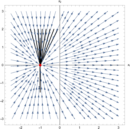
In all cases, the trajectories with initial conditions near the Big Rip de Sitter fixed point values, tend asymptotically to the fixed point, which is stable. This means that once the trajectories are attracted to the fixed point, they remain there permanently.
Now let us address another important issue, namely that of the behavior of the gravity function near the Big Rip singularity. As it is conceivable, only approximate forms of gravity can be obtained due to the complexity of the field equations. To this end, we shall utilize the functional forms of the fixed point variables, namely and their definition in terms of the gravity function and the Hubble rate. Since asymptotically we have we get,
| (523) |
hence, by using Eq. (516) and also the fact that at leading order near the Big Rip singularity the Ricci scalar at leading order is,
| (524) |
we get the following solution for the derivative of the gravity function,
| (525) |
with being an arbitrary integration constant, and the parameter is equal to,
| (526) |
Upon integration of Eq. (525) with respect to , we get the functional form of the gravity as the Big Rip singularity is approached, which is,
| (527) |
with being an arbitrary integration constant. We can further simplify the gravity utilizing the fact that as , the Ricci scalar blows up , and also due to the fact that , the gravity of Eq. (527) can be further approximated as,
| (528) |
We need to note that for consistency we need to require that the parameter has the form , with and being positive integers. The resulting expression for gravity in Eq. (528) is functionally similar to the ones found in Refs. Bamba:2008ut; Nojiri:2008fk, however, the general analytic treatment of finding the gravity near general forms of singularities could be quite demanding.
To recapitulate the findings of this section, let us highlight the most important findings. As a Big Rip singularity is approached, the gravity dynamical system becomes asymptotically autonomous, and its solutions tend asymptotically to the stable de Sitter fixed point of the autonomous gravity dynamical system for a de Sitter evolution. This is quite remarkable and it indicates two things: firstly and more importantly that the Universe as it approaches a Big Rip singularity driven by an gravity, it approaches in an accelerating way. Simply state that in gravity, a Big Rip singularity is approached during the DE era. Secondly the fact that the autonomous de Sitter gravity dynamical system and the gravity dynamical system near a Big Rip singularity, which is render autonomous near the Big Rip singularity, share the same fixed point solution, or stated differently, the same final attractors in the theory. Let us note that in general, the addition of an term in the gravity Lagrangian may significantly affect the development of the singularity since terms are known that they remedy finite-time singularities Bamba:2008ut; Nojiri:2008fk; Capozziello:2009hc; Nojiri:2009pf; Elizalde:2010ts. In addition, the combined presence of an term may provide a unified description of inflation with DE era Bamba:2008ut; Nojiri:2008fk; Capozziello:2009hc; Nojiri:2009pf; Elizalde:2010ts; Oikonomou:2022tux; Oikonomou:2020qah; Odintsov:2020iui; Odintsov:2020nwm. However, the addition of an term greatly obscures the mathematical appearance of the dynamical system and thus makes it impossible to reveal the behavior of the trajectories in this case.
Finally, let us note that the correspondence between the Einstein and Jordan frames, may reveal important relationships between the two frames, for example a Big Rip singularity in the Jordan frame may correspond to a Type IV singularity in the Einstein frame Bamba:2008hq.
VIII.1.3 The Cases of Type III, Type II and Type IV Singularities
We shall now consider the cases of Type III, Type II, and Type IV singularities, in which cases, as the cosmic time tends to the singularity occurring value , we have that , see Eq. (518). Hence, in this case we have,
| (529) |
with and being positive integers. Let us analyze first the case of the Type III singularity, and since as , the parameter defined in Eq. (519) diverges. The analytic treatment of both the Type III and Type II singularities is difficult to tackle, however, for the case of the Type IV singularity, things are easier, in the case that . In this case, becomes and thus the dynamical system (VIII.1.1) has the solutions , , and which are identical with the ones in Eq. (VIII.1.2), for a general , but for the case at hand, at , the parameters , , and become,
| (530) |
and therefore, as , the trajectories of the dynamical system approaches in the phase space. It is noticeable that although and diverge as the singularity is approached, the Friedmann constraint is still satisfied because the singularities in the variables and cancel. We can reveal the functional form of the gravity near the Type IV singularity, simply by solving the differential equation which stems form the condition . Following the same procedure as in the Big Rip case, as we have at leading order,
| (531) |
hence, the derivative of the gravity reads,
| (532) |
with being an integration constant and the parameter is,
| (533) |
The integration of Eq. (532) yields the following functional form of the gravity,
| (534) |
with being an integration constant. We can further simplify the above functional form of the gravity by exploiting the fact that as the Ricci scalar tends to zero because , hence, we have at leading order,
| (535) |
Furthermore for the extremely soft Type IV singularity , we have,
| (536) |
VIII.1.4 The Case of non-vacuum Gravity
In the previous subsections we considered the dynamical system of gravity near finite-time singularities in the absence of matter perfect fluids. In this subsection, we shall consider the inclusion of perfect matter fluids in the dynamical system of gravity. As we shall evince, this will perplex things in the dynamical system when finite-time singularities are approached. With regard to perfect fluids we shall consider non-relativistic matter and radiation perfect fluids. In the presence of matter perfect fluids, the field equations of gravity for a FLRW metric read,
| (537) | ||||
| (538) |
with and being the total effective energy density and the total effective pressure of all the matter fluids present. In this case we introduce the following dimensionless variables,
| (539) |
where and respectively denotes the energy density of radiation and the matter fluid. In the presence of matter fluids, using Eqs. (537) and the variables (539), the dynamical system (VIII.1) of the vacuum gravity takes the following form,
| (540) |
where the parameter is defined in Eq. (511). In the case the Hubble rate is given in Eq. (516), the parameter is given in Eq. (519), but in this case, the dynamical system cannot be analytically solved even in the limiting cases of the parameter considered in the previous subsections. In addition it is impossible to reveal the behavior of the dynamical system even numerically, except for the variable which behaves in an identical way as in the autonomous dynamical system case. Now let us stress for the first time the difference between a finite-time cosmological singularity and a singularity of the dynamical system variables. If some of the variables of the dynamical system blow up at some finite-time, this singular behavior does not necessarily indicate a finite-time cosmological singularity. Take for example the variable , for the vacuum gravity case. As the Big Rip cosmological singularity is approached, the variable tends asymptotically to the value while when the rest of the finite-time singularities are considered, the variable as the finite-time singularities are approached. Thus, the singularities in the field variables do not necessarily indicate a cosmological singularity, except for the variables and in Eq. (539) which depend explicitly on the energy density. Regarding finite-time dynamical system singularities, these can offer insights toward the complete understanding of the behavior of the trajectories in the phase space. The most formal way to study finite-time dynamical system singularities is by studying the dominant balances of the dynamical system based on a -series approach near a finite-time dynamical system singularity GORIELY2000422, see also Refs. Odintsov:2018uaw; Odintsov:2018awm for recent cosmological applications. This method only applies for autonomous dynamical systems and thus cannot be applied for the gravity case or some other modified gravity. Interacting multifluid cosmologies though are relatively simple theories and their dynamical systems is in most cases autonomous, thus can be studied using the dominant balances method. This is the subject of the next subsection.
VIII.2 Finite-time Cosmological and Dynamical Systems Singularities in Interacting Multifluids Cosmology
The dark sector is composed by the DM and DE fluids, which may or may not interact. The perfect fluids can be different in nature, for example the DE fluid may be generated by some non-trivial underlying modified gravity. Without explicitly using the modified gravity we may model the DE fluid in an agnostic way by a dark fluid which interacts with the other dark sector fluids, such as the one of DM, adding an interaction among them. The interaction between the dark sectors though must carefully be chosen because it may have considerable effects on the primordial matter density perturbations Eingorn:2015rma; Koshelev:2010umw. Both the dark sector fluids though cannot interact with the baryonic perfect fluid in order to avoid unobservable fifth force effects. We shall write the field equations corresponding to the three fluids and we shall form them in an autonomous dynamical system way in order to study its trajectories, its singularities and the connection of finite-time dynamical system singularities with the finite-time cosmological singularities. For the dynamical systems singularities, we shall use the dominant balances method developed in GORIELY2000422 which we shall briefly review.
For a flat FLRW metric, the three fluid cosmological field equations in a modified gravity cosmology context reads,
| (541) |
with denoting the total energy density of the cosmological fluids where , , are respectively the energy density of the pressureless DM, DE and baryons. Now, differentiating Eq. (541) with respect to the cosmic time and using the conservation equation for the total fluid we get,
| (542) |
with being the total pressure of the fluids, which basically consists of the pressure of the DE fluid since DM and baryons are pressureless. For the DE sector, we shall consider a generalized EoS of the form Nojiri:2005sr,
| (543) |
with being a real dimensionless parameter. From the energy-momentum conservation equations, we have,
| (544) |
where denotes the interaction term among the DE and DM fluids and the sign of determines which fluid gains energy at the expense of the other fluid which loses energy. Here, implies that energy flow takes place from DE to DM (i.e. DE fluid loses energy and DM fluid gains energy) and indicates that energy flows from DM to DE (i.e. DM fluid loses energy and DE fluid gains energy). We shall assume that has the following form,
| (545) |
which has many phenomenological supports Caldera-Cabral:2008yyo; Pavon:2005yx; Quartin:2008px; Sadjadi:2006qp; Zimdahl:2005bk. Note that , , are the coupling parameters of the interaction model (545) and they are real constants. We can construct an autonomous dynamical system for the cosmological system at hand based on the equations (541), (542), and (VIII.2), so we choose the dimensionless variables of the dynamical system as follows,
| (546) |
The variables of the dynamical system satisfy the Friedmann equation, which is the case at hand is,
| (547) |
Also the total EoS, , of the cosmological system, is also expressed in terms of the variables of the dynamical system in the following way,
| (548) |
In view of the cosmological equations (541), (542), and (VIII.2) considered together with the dynamical system variables (546), we get
| (549) |
which hold true for a general interaction term . Also we used the -foldings number as a dynamical variable instead of the cosmic time. If we use the form of the interaction term , we further have two terms in the dynamical system (VIII.2), which are
| (550) |
hence, the dynamical system (VIII.2) has two additional linear contributions for the dynamical system variables and .
VIII.2.1 Singularity Structure of Autonomous Dynamical Systems Using the Dominant Balances Technique
In this subsection we shall introduce the dominant balances technique for studying the finite-time singularities of polynomial autonomous dynamical systems of an arbitrary dimension. This method was introduced by GORIELY2000422, and the theorems that apply may specify the nature of the finite-time dynamical system singularities. Extra work is required in order to reveal whether a finite-time dynamical system singularity is a physical finite-time cosmological singularity though. For brevity we shall refer to the dominant balances framework as “dominant balance analysis”. Let a general a -dimensional dynamical system having the following form,
| (551) |
with being some real vector of , and also is some vector containing polynomials of . A finite-time singularity developed by this dynamical system is some sort of a moving singularity, which is always related to and determined by the initial conditions of the vector . We can quantify the terminology moving singularity, which is a singularity of the form , with being simply an integration constant. An example is given by the differential equation , which has the solution , with being an integration constant. This solution develops a singularity which mainly depends on the chosen initial conditions, at , so this justifies why it is called a moving singularity. Now in order to find whether the autonomous dynamical system (551) develops finite-time singularities is predominantly based on the decomposition, or simply truncation, of the function in several possible dominant and subdominant terms, which we will denote as and , so in effect the dominant terms of the dynamical system yield,
| (552) |
The dominant terms of the function can be chosen in several ways, and also recall that one polynomial term is allowed to be inserted in the dominant vector each time. Each component , of the vector is written as follows,
| (553) |
and also notice that we require that the full dynamical system solution may be written in a form of -series in terms of , with being the time instance that the singularity occurs. Upon substituting the forms of the solutions ’s of Eq. (553), in Eq. (552), we equate the powers at each order of the resulting polynomials, for each distinct choice of . By using this procedure, we will be able to determine the parameters , by having in mind that the sole solutions accepted are fractional numbers or integers. Accordingly, we form out of the the new vector , which is an important ingredient of the method we apply. Accordingly we find the parameters , which can be determined in a unique way by simply equating the coefficients of the polynomials that result from the dominant part . Using these coefficients we form the vector , which is called dominant balance. For the dominant balance analysis, only non-zero values of the balances are allowed, real or even complex numbers. The two vectors and form the balance . Now following the theorem developed by Goriely and Hyde in GORIELY2000422, we have that if the dominant balance contains complex entries, then the autonomous dynamical system under consideration (551) develops no finite-time singularities. In the case that the dominant balance entries are real, then in principle finite-time singularities occur in the dynamical system, meaning that some trajectories in the phase space will certainly blow-up for some initial conditions. But the question is whether these initial conditions that drive the singular trajectories, are generic or correspond to a limited set of initial conditions. In order to further enlighten this situation, one needs extra criteria that need to be fulfilled. To this end, we construct the Kovalevskaya matrix , defined in the following way,
and it should be evaluated at each non-zero dominant balance found earlier in the method. The eigenvalues of the Kovalevskaya matrix then, should be of the form . Now in the case that the are positive, the dynamical system of Eq. (551) has general trajectories-solutions which will definitely develop a finite-time dynamical system singularity. In this case, all the initial conditions used in this case, drive the dynamical system to a finite-time dynamical system singularity. One the other hand if one of the eigenvalues turns out to be negative, in this case only a limited set of initial conditions will lead the trajectories to a finite-time singularity, since the solution found is not general. It is noticeable that if a singularity is developed by the dynamical system, then the singularity occurs in the same orthant of in the -dimensional phase space spanned by the variables . Practically, this means that if the dominant balance value is negative, then the singularity occurs at the orthant in the space of the dynamical system variables. Let us here provide a simple example of how the dominant balance method works, and to this end consider the dynamical system,
| (564) |
with . From the r.h.s. of the above dynamical system, we can form the following 2-dimensional vector field ,
By applying the dominant balances method, we find easily that the only truncation which is dominant, denoted as , is the following,
and note that this dominant balance results in an acceptable dominant balance . Specifically, the only balances found, denoted as and , are the following,
| (569) |
Accordingly, the evaluation of the Kovalevskaya matrix leads to the eigenvalues and , hence, due to the main theorem related to the Kovalevskaya matrix, we find that the autonomous dynamical system (569) contains solutions that for general initial conditions are attracted to a finite-time singularity.
VIII.2.2 Dominant Balance Analysis of Multifluid Cosmology, Dynamical System Finite-time Singularities versus Physical Finite-time Singularities
The analysis that follows was firstly considered in Ref. Odintsov:2018uaw. In general, the functional form of a cosmological dynamical system variable may reveal whether a dynamical system finite-time singularity may or may not be related to a physical finite-time singularity. Let us consider the variables (546) and apparently, if the variable for example is finite in terms of , then the quantity is finite. In such a case, if one of the variables diverges, then this would simply imply that one of the following energy densities , , or diverges.
In turn, such a situation would imply the occurrence of a Big Rip or a Type II singularity in general, however, in reality things are more complicated that it seems. Considering the Friedmann constraint (547) which is satisfied by all the variables (), for all the -foldings numbers, if finite-time singularities occur in the variables (), then these must occur in such a way so that the infinities cancel and the Friedman constraint is formally satisfied. From a physics standpoint, we first consider the case that the baryon density is finite, thus we shall seek singular behaviors in the dark sector variables and , in which case these would cancel in the Friedmann constraint. Thus the singular behavior would occur in such a way so that the singularities of the dark sector variables and cancel when their sum is considered. For the corresponding dominant balances, this would simply imply that and furthermore . If a finite-time singularity is found in , then the singularities should also occur in the dark sector variables, so that the Friedmann constraint is finite. Also note that if is singular, this indicates a physical singularity for sure, most likely a Type II, a Big Rip, or Type III. Furthermore, let us not that in all cases the variable must be positive. Apparently, the most easy case to handle mathematically is the occurrence of a finite-time singularity in the variable . This would signify a pressure singularity probably.
In conclusion, the only case that a singularity is acceptable that can be verified for sure, is if the variable diverges at finite-time, and in turn this would indicate the possible presence of a finite-time singularity. The type of physical cosmological singularity that occurs in depends strongly on the dependence of the Hubble rate on the -foldings number . Let us see this by using the Hubble rate (516), which expressed in terms of the -foldings number , takes the form,
| (570) |
In the case of a Big Rip singularity () and also for the case of a Type III singularity (), as , we have that , hence, the Hubble rate diverges as the singularity is approached . For both the Type II and Type IV cases, the Hubble rate tends to zero. Thus a singular behavior of the dynamical system variable , indicates either a Big Rip or a Type III singularity physical cosmological singularity. Hence, with certainty, the only case that a dynamical system singularity indicates a physical cosmological finite-time singularity is when diverges. It is noticeable that when the Hubble rate diverges, in which case a singularity in is developed, the term tends to zero, when , in the Big Rip case and when , for the case of the Type III singularity. Therefore, the dark sector dynamical system variables and are finite when a Big Rip or a Type III singularity is developed. We used this characteristic example just to make the point stronger, although the Hubble rate (516) is not a solution of the cosmological system. The most difficult dynamical system singularities to interpret are singularities occurring in one of the dark sector dynamical system variables and , since it is hard to know if a physical singularity occurs when these two blow-up. The only certain about the latter case is that the singular behavior must definitely cancel when the sum is considered. Below we summarize the main outcomes of the above discussion when the dynamical system (VIII.2) is considered:
- •
Singularity in : This indicates a physical singularity, either a Big Rip or Type III.
- •
Singularity in and : Dynamical system singularities, we must have, and .
- •
Singularity in : This is not possible.
- •
Constraints on : always and non-singular.
- •
Singularities in and : If develops a singularity, then and diverge in such a way so that and are singular, and these two must satisfy . If the variable is regular, and furthermore and are singular, then and are not necessarily singular, but they must satisfy .
We note that for all the above cases, the Friedmann constraint must hold true. Now, in the following, we shall analyze the dominant balances and the corresponding singularities of the multifluid system we considered previously. Before going to that, we will make some clarifications. Firstly we shall assume that , , , and , near the possible finite-time dynamical system singularities, behave as follows at leading order,
| (571) |
hence, we shall seek for dominant balances , with the vectors and having the form,
| (572) |
We can rewrite the dynamical system (VIII.2) in the form , with , and also the function is defined as,
Therefore we shall seek for all the consistent truncations of the vector defined in Eq. (VIII.2.2), and using the method of dominant balances we shall examine the behavior of the dynamical system near finite-time singularities.
VIII.2.3 Consistent Truncation I
One truncation of (VIII.2.2) has the following form,
hence, by following the procedure we developed previously, we find the following solution for the vector ,
| (581) |
In the same way, for the above , we find the following solutions and
| (582) |
and the corresponding Kovalevskaya matrix for the truncation (VIII.2.3) has the following form,
We can find the Kovalevskaya matrix for each of the vectors appearing in Eq. (582), hence, for , the Kovalevskaya matrix has the following form,
and also the corresponding eigenvalues for the vector are,
| (591) |
The Kovalevskaya matrix for the vector , has the same form as for the vector , and also the same eigenvalues. In effect, the truncation (VIII.2.3) shows us that the Kovalevskaya matrix contains, apart from , other negative eigenvalues, meaning that the singularities do not occur for the general set of initial conditions.
VIII.2.4 Consistent Truncation II
We can form the second consistent truncation of (VIII.2.2) as follows,
which results in the following vector ,
| (596) |
and now there is only one vector
| (597) |
In the same way, for the consistent truncation (VIII.2.4), the Kovalevskaya matrix takes the following form,
which for leads to
and its eigenvalues are,
| (606) |
For the dominant balances, we shall now analyze the development of phase space singularities for the dynamical system (VIII.2). It develops finite-time singularities and further investigation is required in order to see whether these occur for general initial conditions or for limited ones. This will be revealed by the form of the eigenvalues (606), hence, since , this indicates that the singularities do not occur for a general set of initial conditions, but for a limited set of initial conditions. Furthermore, the singularities for the three phase space variables , , and , is not the wanted one, as it can be seen from in Eq. (596). This is due to the fact that at leading order, the exponents of , , and , are not of the same order, hence, the Friedmann constraint of Eq. (547) is not satisfied in this case. Hence, in this case, the limited set which yields singular solutions, does not yield physically acceptable solutions. Therefore, the mathematically consistent truncation (VIII.2.4) does not yield singular solutions which are generated by a general set of initial conditions.
We can form a third consistent truncation of (VIII.2.2), which has the following form,
which results in given by,
| (611) |
while the vectors are,
| (612) |
and the corresponding Kovalevskaya matrix has the following form,
For the vector , the Kovalevskaya matrix takes the following form,
and its eigenvalues are,
| (621) |
Hence, this truncation leads to a situation with degeneracies, thus, let us further analyze the case . As it occurs, the singularity analysis is identical with the truncation (VIII.2.4). Therefore, no general initial conditions can lead to singularities in the dynamical system in this case too, and furthermore, the singular solutions are non-physical since the Friedmann constraint (547) is not satisfied. The conclusion of this section is that the dominant balance analysis does not yield any singular solutions which are generated by general initial conditions. Thus, it is rather compelling to present in more detail the phase space of the dynamical system, which we do in the next subsection.
VIII.2.5 Phase Space Analysis of Multifluid Cosmological Model
Now we shall analytically investigate the phase space structure of the dynamical system in order to further understand the various phase space structures that emerge in it. We will focus in finding the fixed points of the dynamical system and we shall examine the stability of the fixed points against linear perturbations, by using the well-known Hartman–Grobman theorem, when it applies. The standard way to analyze autonomous non-linear dynamical system is based on the linearization techniques essentially quantified by the Hartman–Grobman linearization theorem. The latter reveals the stability of the various fixed points and further indicates whether non-trivial topological structures exist in the phase space of the dynamical system, only in the case when the fixed points are hyperbolic. Let us describe in brief the theoretical approach we shall use. Consider the vector field , which satisfies the differential flow,
| (622) |
with being a locally Lipschitz continuous map having the form . Let the fixed points of the dynamical system (622) be denoted as and also let denote the Jacobian matrix which corresponds to the linearized version of the dynamical system (622) near some fixed point, with the Jacobian matrix being equal to,
| (623) |
In the case of a fixed point being hyperbolic, the Jacobian matrix evaluated at the fixed point reveals the stability of the fixed point. Let us remind here that a fixed point is called hyperbolic only if the spectrum of the eigenvalues of the Jacobian matrix is comprised by elements satisfying the condition . In this case, following the Hartman–Grobman theorem, the linearized version of the dynamical system,
| (624) |
is equivalent topologically, to the dynamical system of Eq. (622), at the vicinity of the hyperbolic fixed points . Specifically, the Hartman–Grobman theorem guarantees the existence of a homeomorphism , in a neighborhood of the hyperbolic fixed point , with being an open set. This homeomorphism generates the flow , satisfying,
| (625) |
In view of the Hartman–Grobman theorem, the flows in Eqs. (625) and (622) are homeomorphic. Now regarding the stability of the fixed point , the Hartman–Grobman predicts that in the case that the spectrum of the eigenvalues of the Jacobian matrix are negative, that is , then the fixed point is stable asymptotically. In all the other cases, the fixed point leads to instabilities in the phase space. We shall now apply the Hartman–Grobman theorem on the dynamical system of Eq. (VIII.2) with the interaction term being chosen as in Eq. (545). We shall calculate the fixed points and we examine their stability against linear perturbations. Our analysis indicates that for general non-zero values of , the analytic study of the fixed points is very complicated and somewhat leads to extended and complicated. So we shall focus on the case . Interactions like the one in (545), with are frequently used in the literature Boehmer:2008av. The case with can be dealt numerically, and in TABLE 5, we gather our results, for various signs of the free parameters and of the interaction function (545). For all the cases appearing in the TABLE 5, the distinct fixed points and physically interesting fixed points are unstable, without the result to be dependent on the values of the free parameter .
| Case No. | Region of and | Nature of Fixed Points |
|---|---|---|
| Case I | , , for every | Unstable |
| Case II | , , for every | Unstable |
| Case III | , , for every | Unstable |
| Case IV | , , for every | Unstable |
Now let us consider the analytic form of the fixed points for , in which case the fixed points are,
| (626) |
The Jacobian matrix for the current scenario, has the simple closed form,
For the last two cases, the fixed points correspond to de Sitter vacuum, since we have at the two fixed points. Regarding the other cases, the variable is equal to zero at the fixed point, hence, the most interesting cases from a phenomenological point of view correspond to and , for which tends to zero. Hence, in this case, asymptotically near the fixed point, the baryonic fluid does not contribute to the dynamical evolution of the Universe, asymptotically near the two fixed points. Furthermore, in order to be consistent physically, the interaction constant must be . The eigenvalues of the Jacobian matrix evaluated at the fixed points, for the first four fixed points, have the following form,
| (631) |
Regarding the first two fixed points, these are not hyperbolic, hence, we cannot use the Hartman–Grobman theorem for analyzing these two. In contrast, the fixed points and are hyperbolic, but not stable because some eigenvalues are positive. Hence, in this case the fixed points are unstable but physically appealing because these lead to a Hubble rate that tends to zero, so this might describe the late-time era.
Now we turn our focus on the fixed points and in which case, the calculation of the eigenvalues results in a complicated algebraic equation, which is too extended to present here. By doing a numerical analysis though, for and for being positive and negative, we end up with unstable de Sitter fixed points. The instability can be easily explained due to the fact that enters the EoS as and not as , hence, instability occurs.
Also, a detailed analysis of the trajectories for the dynamical system at hand verifies the above findings. Indeed, for a wide range of values of the free parameters and indicates that there exist limited initial conditions which lead to dynamical system blow-ups at finite-time. Also, there are regions in which the dynamical system has regular trajectories, a fact which is also supported by the stability study of the fixed points. Concluding, the dynamical system (VIII.2) which describes a multifluid cosmology with non-trivial interactions between the dark sector fluids, is unstable in general and has no global attractors leading to finite-time singularities, but has limited trajectories leading to finite-time blow-ups of the dynamical system variables.
VIII.3 Dynamical System Analysis of Exponential Quintessence DE Models
In this section, we shall analyze the dynamical system of exponential quintessence models, which are relevant in swampland models. For a full analysis of this model, see Odintsov:2018zai, on which the presentation of this subsection will be based. Consider the action of a quintessence scalar field model in vacuum,
| (632) |
The field equations for this quintessence scalar theory in a flat FLRW background are,
| (633) |
with the prime denoting differentiation with respect to . We shall be focusing on exponential quintessence models, hence, the scalar potential takes the form . For this choice of the potential, the field equations (VIII.3) can form an autonomous dynamical system by introducing the dimensionless variables,
| (634) |
with the “dot” indicating the differentiation with respect to . As in the previous sections, we shall use the -foldings number to quantify the dynamical evolution variable, so by combining Eqs. (VIII.3) and (634), we can form the following autonomous dynamical system,
| (635) |
Furthermore, the dimensionless variables and satisfy the Friedmann constraint,
| (636) |
which means that in the variables and the dynamical system does not develop singularities. The phase space structure of this simple autonomous dynamical system has been performed in detail in Ref. Agrawal:2018own.
VIII.3.1 Singularity Structure of the Dynamical System Describing Swampland DE Models
In this subsection, we shall use the dominant balance analysis described in a previous section for the dynamical system of Eq. (VIII.3), with the Friedmann constraint (636) holding always true. For doing so, we recast the dynamical system of Eq. (VIII.3), in the following form,
| (637) |
with , and furthermore, we defined the vector-valued function as follows,
with the ’s appearing in Eq. (VIII.3.1) being equal to,
| (640) |
We can form several truncations of this vector function , one of which is the following,
By using the method of dominant balances, we find for this truncation that the vector takes the form,
| (643) |
and accordingly, the following non-trivial vector is obtained,
| (644) |
All the vectors found above have complex entries, and also the Friedmann constraint (636) is satisfied for all the vectors . Indeed, at leading order, the expression forming the Friedmann constraint at leading order reads,
| (645) |
which vanishes, and we should note that . Now let us investigate whether singular solutions can be found. Due to the fact that the vectors have complex entries, this indicates that no singular solutions exist, as we have already shown from the Friedmann constraint (636). What now remains to check is whether these solutions are general or not, meaning whether these correspond to general initial conditions or not. The answer to this will be given by the evaluation of the Kovalevskaya matrix , for the solutions , and for the truncation (VIII.3.1),
The evaluation of the Kovalevskaya matrix for , yields,
the eigenvalues of which are,
| (650) |
The same set of eigenvalues are found for all the rest of solutions ,. The form of the eigenvalues indicates that the dynamical system (VIII.3) has not finite-time singularities, and also these non-singular solutions correspond to a general set of initial conditions. However, these non-singular solutions found do not exclude the existence of an actual physical cosmological finite-time singularity. What we proved is that the dynamical system variables and do not become singular for a general set of initial conditions, which does not exclude the case that an actual physical singularity may be developed. In order to investigate the occurrence of physical singularities, let us assume that the Hubble rate has the general form,
| (651) |
with the parameter taking the general form , and are positive integers, and also and are assumed to be regular at and furthermore, for consistency , . Moreover, the first and second order derivatives of and are assumed to satisfy the same constraints. Although that the Hubble rate (651) may not be a solution to the field equations, we will examine the case that the dominant part of the solution is of the form (651) near a singularity. The results of the singularity structure of the dynamical system indicate that and , never become singular for all the cosmic times. Now, the singularity structure of the Hubble rate (651), strongly depends on the values of and specifically,
- •
If , a physical Big Rip singularity is developed.
- •
If , a physical Type III singularity is developed.
- •
If , a physical Type II singularity is developed.
- •
If , a physical Type IV singularity is developed.
By combining Eqs. (VIII.3) and (651), we can express the terms and as functions of the Hubble rate. Indeed, the two equations needed are,
| (652) | ||||
| (653) |
but the resulting expressions are too lengthy to quote here. Having though these expressions at hand, we shall investigate the occurrence of physical singularities, having in mind that the variables and never become singular for the dynamical system at hand. Considering the case of a Type IV singularity, this can never occur when , since the term is present in the variable . On the contrary, when , the two variables , never become singular, so in the case of a Type IV singularity, this can be developed by the physical system for the values of in the range . Regarding the Type II case, which recall that it occurs for , the dynamical system variable is singular in this case since it depends on the term , therefore a Type II singularity can never occur for the model at hand. Regarding the Type III case, it cannot also occur due to the term , which is singular for . Regarding, the Big Rip singularity, it can always occur, because for , the dynamical system variables and never develop singular behavior. The results of our analysis are presented in TABLE 6.
| Type of the Singularity | Occurrence/Non-occurrence |
|---|---|
| Type I | It occurs for |
| Type II | Does not occur |
| Type III | Does not occur |
| Type IV | Does not occur for , but occurs for |
Therefore, in conclusion, if the dominant behavior of the Hubble rate solution for the model at hand is given in Eq. (651), the Type III, and Type II never occur in the physical system. However, the Type IV and Type I singularities occur when and for any , respectively.
VIII.4 Dynamical System of Interacting Multifluids in LQC
In this section, we shall investigate the occurrence of finite-time singularities in the context of a LQC interacting multifluid system. The full analysis of the subject of this section was performed in Ref. Odintsov:2018awm on which the presentation will be based. The three fluids that are considered are a non-interacting baryonic fluid and the interacting DE-DM fluids. Also the DE fluid will contain a bulk viscosity term. The Friedmann equation in the context of LQC in the presence of the three fluids and for a FLRW spacetime, has the following form,
| (654) |
where, once again, denotes the critical density of LQC and is the total energy density of all the three fluids present in which , and denote the energy density of DM, DE and baryons, respectively. Upon differentiation with respect to the cosmic time, Eq. (654) yields,
| (655) |
where denotes the total pressure of the three fluids, which is basically equal to the pressure of the DE fluid, since DM and the baryonic fluids are pressureless. For the DE fluid, we assume the following EoS Nojiri:2005sr,
| (656) |
with being a real dimensionless parameter. The energy-momentum conservation yields the following three continuity equations,
| (657) |
where denotes the interaction between the dark fluids, and once again indicates that the DE fluid loses energy and indicates that the DE fluid gains energy at the expense of the DM fluid. We shall consider the following interaction between the dark sector fluids,
| (658) |
which is phenomenologically interesting Caldera-Cabral:2008yyo; Pavon:2005yx; Quartin:2008px; Sadjadi:2006qp; Zimdahl:2005bk and here , are the coupling parameters. For the three-fluid LQC system with equations (654) and (655), we can construct an autonomous dynamical system by appropriately introducing some dimensionless variables. After this, we shall investigate whether the resulting polynomial dynamical system develops singularities at some finite-time, using the dominant balance technique we presented in previous sections of this chapter. We shall also discriminate the dynamical system singularities from the actual physical finite-time singularities. The major outcome of this section is the fact that we shall analytically prove that the resulting LQC dynamical system has no finite-time singularities, which verifies that LQC actually leads to non-singular behavior. We now construct the autonomous dynamical system from Eqs. (654), (655) and (657). We choose the dimensionless dynamical system variables as follows,
| (659) |
which are constrained to satisfy the Friedmann constraint,
| (660) |
for all cosmic times. Furthermore, the total EoS parameter corresponding to the multifluid system, expressed in terms of the dimensionless dynamical system variables (659), takes the following form,
| (661) |
Now we can form the polynomial autonomous dynamical system for the three multi-fluids system, by combining Eqs. (654), (655), (657), and (659), so after some algebra, we get,
| (662) |
and note that, as in the previous sections in this chapter, we used the -foldings number to quantify the dynamical evolution of the variables, instead of the cosmic time. Furthermore, by choosing the interaction term as in Eq. (658), the -containing terms in the dynamical system (VIII.4), can be expressed in terms of the variables and in the following way,
| (663) |
Now having the dynamical system (VIII.4) at hand, we can apply the dominant balance analysis in order to reveal the dynamical system singularities and we shall also investigate whether physical singularities occur too. This is the subject of the next subsection.
VIII.4.1 Dominant Balance Analysis of the three-fluid Cosmological Dynamical System
We shall use the method of dominant balances in order to investigate whether the dynamical system (VIII.4) develops finite-time singularities. As we shall show, the dynamical system is singularity-free and in fact this result holds true for a general set of initial conditions. One should have in mind of course that there exists a limited set of initial conditions that may lead in principle to finite-time dynamical system singularities, but this limited set is not of interest. Near a singularity, the dimensionless variables , , and at leading order behave as follows,
| (664) |
The dynamical system (VIII.4) can be rewritten as follows , with being , and also is defined to be equal to,
and the corresponding functions , are,
| (669) |
Now we shall seek for consistent truncations of the vector-valued function defined in Eq. (VIII.4.1), and investigate whether singular solutions exist or not. Among many distinct truncations of the vector function , one is the following,
The corresponding vector , which obviously corresponds to the solution , is easily found,
| (674) |
and the corresponding vectors are,
| (675) |
The corresponding Kovalevskaya matrix is given by
with eigenvalues
| (680) |
In conclusion, the major outcome of this section is the fact that LQC utterly erases any finite-time singularities that may have occurred in the classical interacting three fluid system. We have to take into account that the variables diverge when the Hubble rate vanishes, and this happens when or . That means, the singularity, in the variables, exhibits that the total energy density coincides with the critical one, and thus, this singularity in the variables is not a physical singularity in the sense that neither the Hubble rate diverges nor the corresponding energy densities diverge for our interacting three fluid system in the context of LQC.
We shall conclude the analysis by finding analytically the fixed points of the dynamical system. Also, we shall reveal the behavior of the total EoS parameter of Eq. (661), in terms of the coefficients and appearing in the interaction term . We can find the fixed points of the dynamical system which well-known linearization techniques for dynamical systems. In the case that the fixed point is hyperbolic, in which case the eigenvalues of the matrix that results after the linearization of the dynamical system contain non-zero real part, the stability of the fixed point can be determined. In the case of a hyperbolic fixed point, when the eigenvalue of the linearization matrix has a negative real part, then the fixed stable, and if the real part is negative, then the fixed point is unstable. We shall denote the fixed points of the dynamical system (VIII.4) as , and the Jacobian of the linearized dynamical system near the fixed points as, , with the latter being equal,
| (681) |
Now we shall solve the equation , with appearing in Eq. (VIII.4.1), and this process will reveal the fixed points of the dynamical system (VIII.4), which are,
| (682) |
Apparently, the fixed points and are not hyperbolic, and the fixed points , and are hyperbolic. Omitting the exact form of the eigenvalues for brevity, a thorough analysis of the phase space indicates that the fixed points are unstable, regardless the values of the parameters , , . Also the total EoS in Eq. (661) must be studied for various values of the free parameters. We shall consider the case that we fix the DE EoS parameter to have various values, varying from quintessential values () to phantom values (). A numerical analysis of the total EoS parameter (661) indicates that in the context of the three fluid interacting cosmology, it is possible to realize various cosmological evolutions, for example quintessential, phantom and also matter dominated eras.
VIII.4.2 The Choice of the DE EoS and its Physical Implications
For the analysis performed in the previous subsections, the choice of the DE EoS was chosen to be that of Eq. (656). However, a more general EoS can be used, which may include higher powers of the Hubble rate and also further effects of viscosity might be included. In this subsection we report the implications of the chosen EoS (656) for DE phenomenology. Using the formalism of Astashenok:2012iy which we extend in the context of LQC, a comparison of the classical theory with the LQC one can be done for the chosen EoS (656). We note that when the LQC effects are not considered, the EoS of Eq. (656) drives the cosmological system to finite-time singularities of the Type III form Nojiri:2005sx. On the other hand, in the case of LQC, with one fluid, the singularities are eliminated Sami:2006wj, and as we demonstrated previously, the same applies in the three fluid system in which DM and DE are interacting with each other. Thus, LQC eliminates the finite-time singularities. Our findings and comparisons are presented in TABLE 7.
| Case Study | Cosmological Scenario | Occurrence of Singularities |
|---|---|---|
| Classical Case | Interacting Multi-fluids | Type III singularity occurs |
| LQC | One DE Fluid | No singularity occurs |
| LQC | Interacting Multi-fluids | No singularity occurs |
IX The Avoidance of Finite-time Future Singularities
Near the singularity, especially in the case of Type I and Type III, the Hubble rate becomes very large, which means that the curvature and the temperature become very large and therefore the quantum effect and the thermal effect become important. One may naturally wonder whether it is possible to avoid the finite-time singularities from the cosmological picture so that we realize a non-singular Universe. In this section, we shall examine the possibility of avoiding the finite-time singularities in the cosmological scenarios. More specifically, we shall discuss what could happen with the future singular dark Universe when the effects of quantum or thermal radiation are included. This section is based on Refs. Frampton:2011sp; Brevik:2011mm; Nojiri:2020sti; Carroll:2003st.
IX.1 Little Rip Scenario
The possibility of a phantom DE EoS (i.e., ) is very hard to exclude from the cosmological picture DiValentino:2020vnx. The phantom DE can solve the Hubble constant tension DiValentino:2021izs quite excellently. However, one of the serious features that the phantom DE carries is the following. For , the DE density increases with the increasing scale factor and both of them can blow up at some finite-time in the future leading to a Big Rip singularity Caldwell:2003vq. However, this future singularity can be avoided even if and this heuristic scenario, dubbed as “Little Rip” was introduced in Ref. Frampton:2011sp. With such fantastic proposal, the Little Rip scenario received significant attention to the scientific community Frampton:2011sp; Brevik:2011mm; Frampton:2011rh; Nojiri:2011kd; Granda:2011kx; Ito:2011ae; Xi:2011uz; Liu:2012iba; Saez-Gomez:2012uwp; Brevik:2012nt; Brevik:2012ka; Balakin:2012ee; Frampton:2013fxa; Makarenko:2014nca; Bouhmadi-Lopez:2014cca; Albarran:2015cda; Morais:2016bev. In this section, we shall describe how the Big Rip singularity could be avoided even if is less than .
In order to realize a non-singular scenario, one can proceed with a non-singular scale factor having the following form
| (683) |
where is any arbitrary non-singular function satisfying . From the Friedmann equation , one can derive that . And from the condition that is an increasing function of which implies , gives the restriction
| (684) |
because we are dealing with an expanding Universe, i.e., with . Thus, one may note that all Little Rip scenarios which are described by the evolution of the scale factor given by Eq. (683), with non-singular should satisfy the Eq. (684).
To proceed further in this direction, let us now consider the well-known non-linear EoS Nojiri:2005sr
| (685) |
where ensures that the increases with the scale factor, because in that case . From the conservation equation, , one can find the scale factor as
| (686) |
where we set , the present value of the scale factor to be unity and denotes the present value of the energy density. Now, using the conservation equation and the Friedmann equation , one finds
| (687) |
We assume that is given by the power law , where and are constants. We select in the above form (i.e., we consider ) and for which one can find the time from (687) as
| (688) |
which clearly shows that is not reached in some finite-time. That means even if we have but we can avoid the future singularity and it is known as the Little Rip scenario.
Now, solving (686) for , one can express as a function of as Brevik:2011mm:
| (689) |
and consequently, using the first Friedmann equation, one can explicitly find the scale factor in terms of the time as Brevik:2011mm:
| (690) |
which does not exhibit any finite-time singularity in the future.
IX.1.1 Little Rip in Viscous Universe
The Little Rip scenario can also be realized in the viscous Universe as well. We refer to section III.1 for the basic dynamical equations for a viscous Universe. In the viscous Universe, the effective pressure term as in Eq. (36) or (37) which includes the bulk viscosity component plays the crucial role. We generalize (685) in presence of the bulk viscosity as
| (691) |
where notice that we have generalized the last term in the right hand side of Eq. (37) as in which refers to the coefficient of the bulk viscosity. We investigate the cosmological scenario with
| (692) |
For the constant , using the conservation equation , one can find the scale factor as
| (693) |
where we have explicitly set . Further, using the conservation and Friedmann equations, one can express the time as
| (694) |
Now, for the model (in this case, the dimension of , in natural units, is of the Planck’s mass), we can solve
| (695) |
and consequently,
| (696) |
Thus, we can see that in order to realize , is essential. This is the Little Rip scenario in the viscous Universe. However, it is important to mention that the above Little Rip scenario is dependent on the above EoS (691) with the constant .
Interestingly, one can also realize the Little Rip phenomenon in a more generalized scenario where in addition is not strictly a constant. To illustrate this, we consider the following example:
| (697) |
where , and are constants.77 7 One can quickly note that for and , we realize the previous scenario and . Thus, for the above choice, one can solve for the cosmic time as
| (698) |
which can be expressed after integration in terms of the hypergeometric function as
| (699) |
For constant bulk viscous coefficient, i.e., (equivalently, in Eq. (697)) together with in Eq. (697), we obtain (note that in that case and have units of the Planck mass):
| (700) |
and this presents the Little Rip phenomenon because requires , that means the energy density does not diverge at some finite-time Brevik:2011mm.
IX.2 Geometrical invariants to remove the finite-time future singularities
In Section IV we have seen that different modified gravity theories may lead to a variety of finite time future singularities. However, with the proper choice of the geometrical invariants describing the underlying gravitational theory, it is possible to remove such finite-time singularities. In this section we shall describe briefly how one can avoid such finite time future singularities from various modified gravity theories.
In the context of gravity theory, one can reconstruct the gravity models in such a way so that the finite-time future singularities may disappear from the picture. However, such reconstructions should be consistent with the existing theories of the Universe and the reconstructed model should pass the essential tests of gravity. This point was first raised in Ref. Abdalla:2004sw and subsequently discussed in Refs. Nojiri:2008fk; Bamba:2008ut. We recall that the general action of gravity in the Jordan frame that depends solely on the curvature [i.e. Eq. (165) without matter] having the form
| (701) |
Introducing the auxiliary fields , , one can rewrite the action (701) as Eq. (212) and consequently as Eq. (213). Now, using the conformal transformation where , one can obtain the action in the Einstein frame in Eq. (216) and the corresponding potential in Eq. (217) [see section IV.5.1 for more details].
Dealing with the model
| (702) |
we consider the following case , , and and with these choices, the field turns out to be where , and the potential has the following form
| (703) |
Now, since
| (704) |
then there is a branch point, at or where or . For small values of , the behavior of the potential approaches to . However, when is very large, then approaches to a constant, . Also, the potential vanishes at (since , hence, ). Further, looking at the expression for given by
| (705) |
one can notice that has an extremum at . Now, as there is a branch point at , then if we start from the small curvature, the growth of the curvature stops at , where . In fact, at the branch point, where , the mass of becomes infinite since
| (706) |
Note also that when . Then the growth of is finished at . Hence, with the addition of the term, cosmic doomsday does not occur but the Universe ends up in a de Sitter phase.
The same situation arises for the Hořava–Lifshitz gravity too. As explored in Ref. Carloni:2010nx, the Hořava–Lifshitz gravity has a quite rich cosmological structure and the inclusion of in could avoid the finite time future singularities from the picture.
On the other hand, recalling the gravitational theory, it is also possible to construct some models of gravity where the finite-time future singularities can be avoided. We consider the correction of the power law model of Eq.(402) as follows
| (707) |
where (, ) is the correction term. This model has some interesting features. For , all four types finite time future singularities can be avoided in this model Bamba:2012vg. We emphasize that the model where is treated as the correction term, which is obtained for , the minimum integer satisfying the condition , therefore removes all four types of finite time future singularities. This has similarity with the gravity theory where it has been observed that the inclusion of term could cure the finite time future singularities Abdalla:2004sw; Nojiri:2008fk; Bamba:2008ut. Apart from the above models, there are other type of models which can avoid the finite-time future singularities:
- •
Exponential model: In the exponential model of type
(708) where and are nonzero constants, we do not realize any finite-time future singularities Bamba:2012vg.
- •
Logarithmic model: In the logarithmic model of the form
(709) where and are constants, we do not realize any finite-time future singularities Bamba:2012vg.
In the context of non-local gravity (section IV.9), one can also avoid the finite time future singularities. We consider the scenario where a correction term of the form where is any real number, is added to the action (405) as follows Bamba:2012ky:
| (710) |
Along with the two fields , as in section IV.9, introducing a scalar field . the action in Eq. (710) can be expressed as
| (711) |
Note that by varying action (711) with respect to , one obtains and hence by substituting in (711), one gets back (710).
Now, in the context of a flat FLRW universe, the gravitational field equations for the action (710) can be written as Bamba:2012ky
| (712) | |||
| (713) |
where , are respectively the energy density and pressure of the matter sector; and are respectively the contributions from the additional term given by
| (714) | |||
| (715) |
Now, for the Hubble parameter as in (61) or (107), in the limit , of Eq. (714) and of Eq. (715) are approximately given by
| (716) |
| (717) |
We now examine the r.h.s. of Eq. (407) with in Eq. (714). For , , the first term of Eq. (716), i.e. , becomes the leading term. As , and , therefore, this leading term does not vanish, which means that the additional term can remove the finite-time future singularities. On the other hand, for , the second and third terms of Eq. (716) become the leading terms. Again since , , and , hence, these leading terms do not vanish. This means that the additional term can remove the finite-time future singularities.
We remark that similar to the gravity, where the inclusion of a correction term could cure the singularities Bamba:2012ky, in the non-local gravity too, this situation happens.
IX.3 Scalar field models avoiding finite-time future singularities
According to Carroll:2003st, it is possible to construct scalar field phantom DE models where the big rip singularity can be avoided. Considering a phantom scalar field with potential as in Carroll:2003st, in the background of a FLRW universe, the energy density and pressure of the phantom field, are respectively given by Copeland:2006wr
| (718) |
and the equation of state of this phantom field, takes the form
| (719) |
which satisfies if . The equation of motion of the phantom field is given by
| (720) |
where prime denotes the derivative with respect to and denotes the spatial Laplacian, i.e. . In this model scenario, the dynamics of the universe heavily depends on the potential function . As argued in Carroll:2003st, the following gaussian potential has some interesting consequences in the context of finite time singularities:
| (721) |
where and are constants. For this particular choice of the potential, the evolution of the scalar field, the density parameter of phantom scalar field and its equation of state have been numerically investigated in Carroll:2003st. From the evolution of the equation of state , one finds that Carroll:2003st: during the initial stages of evolution, the phantom scalar field is frozen by the expansion and it behaves like the cosmological constant (i.e. ). After that the field starts to evolve quite rapidly towards the maximum of its potential and the energy density of the phantom field becomes dominant where crosses the phantom divide line and becomes more negative. Finally, in the very late phase of the universe, the field comes to rest at the maximum of the potential and the accelerating expansion begins with . In the late phase, as does not go beyond , hence no future singularity appears. In fact, the universe approaches to a de Sitter phase.
On the other hand, it is interesting to note that for (i.e. the Starobinksy model Starobinsky:1980te) where is a dimensionless constant, one can derive the corresponding quintessence scalar field potential of exponential type Chaichian:2022apa. As due to the presence of in , no finite-time future singularities appear Abdalla:2004sw, therefore, we conclude that quintessence scalar field model with exponential potential could avoid the finite-time future singularities.
IX.4 Inhomogeneous equation of state
In the context of various modified gravity theories, using the effective energy density and pressure , one can derive an effective equation of state , see Eq. (169) for the gravity case [while this is true for other gravity theories as well] in which , see Eq. (170). The explicit form of that involves the geometric invariants and their time derivatives is given in Eq. (IV.5). Therefore, the modified gravity theories can lead to various inhomogeneous equation of state parameters depending on the choice of the underlying gravitational theory. In this section we shall investigate the conditions on that may prevent the appearance of finite time future singularities. If Eq. (170) is found to be inconsistent for kind of finite time future singularities, then one can conclude that no finite time future singularities are realized in this case.
We consider the case when evolves as (108). In that case, the r.h.s. of (170) behaves as Bamba:2008ut
Now for , , which correspond to Type I, II and III singularities, notice that the l.h.s. of (IX.4), i.e., of (170) diverges. Thus, in order to avoid the appearance of such finite time singularities, must be bounded and in this case, Eq. (170) becomes inconsistent with the behavior of the r.h.s. of (IX.4).
An example in this direction is the following Bamba:2008ut
| (726) |
where and are positive real numbers and is a constant.
We further note that for corresponding to Type I or III singularity, the r.h.s. of (IX.4) becomes negative. Hence, if is positive for large , we do not realize any finite time future singularity.
Another chance is that if contains the term like , which becomes imaginary for large , then Eq. (IX.4) becomes inconsistent. Thus, singularities where the curvature blows up (Type I, II, III) could be avoided.
We remark that such mechanism could be applied even if we have the phantom EoS, i.e. . In that case one can add an extra term to . Here, and are real numbers. If is considered to be large enough, is not relevant for the small curvature but relevant for large scale and hence the possibility of the curvature singularity is avoided.
IX.5 Future Singularities with the Account of Quantum Effects
In this subsection we will extend our analysis of singularities performed when we have studied semi-classical gravity. It is well known that, when the Universe approaches the future singularity, its curvature and other geometrical invariants grow up. As a result, the quantum effects may change the behavior of the future spacetime singularity. For example, one can show that quantum effects may change the structure of future singularity, see Nojiri:2004ip; Nojiri:2004pf (see also Kamenshchik:2013naa; Bates:2010nv; Tretyakov:2005en; Calderon:2004bi; Carlson:2016iuw). We will use simple qualitative arguments of Ref. Nojiri:2010wj to show the role of quantum effects in conformally-invariant theories to future singularity.
It is well-known that the generalized conformal anomaly has the following form:
| (727) |
where is the Gauss-Bonnet invariant in (152) and denotes the square of the 4D Weyl tensor, given by
| (728) |
In case when matter is conformally-invariant and there appear scalars, spinors, vector fields, () gravitons, and higher-derivative conformal scalars, and , which are obtained using adiabatic regularization, take the following forms,
| (729) |
As given in (729), for the usual matter, is positive and is negative. An exception is the higher-derivative conformal scalar. Note that the value of can always be shifted with the addition of to the classical action.
If one writes the energy density and pressure corresponding to the trace anomaly , then one has . Now with the use of the energy conservation law in the FLRW Universe, one gets
| (730) |
which can be expressed by eliminating as
| (731) |
and with the help of integration, can be found as Nojiri:2005sx:
| (732) |
Now, using the above expression and identifying , we will consider the FLRW equation, later. Before considering the FLRW equation, as in Nojiri:2010wj, however, we first consider the trace of the Einstein equation, for simplicity, by including the trace anomaly, as follows,
| (733) |
Here, refers to the trace of the matter energy-momentum tensor. Now, for the FLRW Universe, and are as follows
| (734) |
What we would like to show is that, if there is a singularity, then the trace equation (734) cannot be consistent. In particular, we will show that the contribution from the conformal anomaly in the r.h.s. of Eq. (733) is more singular than the scalar curvature in the l.h.s. of Eq. (733). Note that a rigorous study on the quantum effects may be done following Carlson:2016iuw, however, this needs an extensive numerical investigations depending on the particles content of the Universe as well as effective dark fluid.
Now we assume that behaves as in (107) or (108) and neglect the contribution from matter and put . In the case of Type I singularity, the scalar curvature , which is given by , behaves as and in the case of Type III singularity, behaves as . On the other hand, in the case of Type II singularity, behaves as . When Type IV singularity appears, if in (108), is finite but if , .
In the case of Type I singularity, near the singularity, , as seen from Eq. (734), the Gauss-Bonnet invariant behaves as and therefore becomes very large and the contribution from the matter in (733) can be neglected. On the other hand, one finds . Then since , becomes much larger than and therefore Eq. (733) cannot be satisfied. This shows that the quantum effects coming from the conformal anomaly remove Type I singularity.
In the case of Type II singularity, we find that behaves as . Since , the Gauss-Bonnet term in is less singular and therefore negligible compared with and the contribution from the matter. Therefore, the Gauss-Bonnet term in does not help to prevent Type II singularity. Note, however, behaves as , which is more singular than the scalar curvature. Then if , the contribution from becomes much larger than near the singularity and Eq. (733) cannot be satisfied. Therefore, if , even Type II singularity can also be prevented when the quantum effects due to conformal anomaly are included.
In the case of Type III singularity, the Gauss-Bonnet invariant behaves as and behaves as . Because the scalar curvature behaves as , both of the terms, and , are more singular than the scalar curvature and Type III singularity is also prevented. Thus, we demonstrated that quantum effects may remove finite-time future singularities. Note that account of quantum gravity effects in specific models is also known to remove the Big Rip singularity Elizalde:2004mq.
IX.6 FLRW equation including Trace Anomaly
Here we consider the FLRW equation including the effective energy density induced by the trace anomaly in (732). By using (727), (734), and (732), we find the explicit form of as follows
| (735) |
Then the FLRW equation is given by
| (736) |
Here is the energy density corresponding to the phantom DE, which behaves as with . By combining (735) and (736) and assuming (we take ), we obtain
| (737) |
Differentiating the above expression with respect to , we obtain
| (738) |
If we assume
| (739) |
with a positive constant , we find
| (742) |
By using the above behaviors, we investigate what kind of singularity can be realized or prohibited.
First, we consider the case of Type I singularity, where . If , the energy density of matter grows up very rapidly when , other terms in (738) cannot cancel the term and therefore Eq. (738) is not satisfied. If , the l.h.s. of (738) behaves as
| (743) |
On the other hand, the first term in the r.h.s. of (738), which comes from the matter, as found in (IX.6),
| (744) |
and the second term in the r.h.s. of (738), which comes from the trace anomaly, behaves as
| (745) |
Because and as in (729) and is arbitrary, as long as , the second term in the r.h.s. of (738) is positive. Compared with (743) and (IX.6), we find that the l.h.s. of (738) cannot balance with the second term in the r.h.s. of (738). Furthermore, because both of the first and second terms of (738) are positive as , they cannot cancel each other. This tells that the behavior with does not satisfy Eq. (738). By combining the results with and , we find that the Type I singularity is prohibited.
We now consider Type III singularity, where . We should note that in Eq. (738), in the limit of , the first term in the r.h.s. is finite and the l.h.s. and the second term in the r.h.s. diverge. Therefore we may neglect the first term in the r.h.s. of (738). Because now , the l.h.s. cannot balance with the second term in the r.h.s. and therefore (738) cannot be satisfied and the Type III singularity is prohibited.
In case of Type II, where , n the limit of , the first term in the r.h.s. is finite, again. On the other hand, in the limit, the l.h.s. (738) diverges as and the second term in the r.h.s. behaves as if , or if , the l.h.s. cannot balance with the second term in the r.h.s. and therefore (738) cannot be satisfied, again and the Type II singularity is prohibited.
By combining the above results, we find the Type I, II, and III singularities are prohibited by the quantum effects coming from the trace anomaly. The Type IV singularity can be allowed in general when there is any matter.
When the matter can be neglected, to see what could happen, we solve (738) by putting and by adjusting so that . Then we can rewrite (738) as follows,
| (746) |
which can be integrated to be
| (747) |
The solution has two branches for positive , that is, the region and . When , goes to the plus infinity and , goes to the plus infinity, again. That is, there is a local minimum in the region . In the region, , when , goes to the plus infinity and after that monotonically decreases as a function of and when , vanishes as . Then there could be three scenarios for the cosmology. In one scenario, the Universe starts from the finite corresponding to the local minimum in the region . After that, there are two possibilities. In one possibility, when increases, and in another possibility, when increases, . In another scenario, the Universe starts at with . After that, monotonically decreases and goes to when .
IX.7 Future Singularities with the Account of Thermal Effects
We may remind that the large Hubble rate means the large temperature of the Universe. The Hawking radiation effectively should be generated at the apparent horizon of the FLRW Universe Gibbons:1977mu; Cai:2008gw. Eventually, it should give an important contribution to the energy density of the late-time Universe, especially right before the Rip time. In other words, at a large temperature that may even diverge at the Rip time, there should appear thermal radiation.
IX.7.1 Type I Singularity with Thermal Effects: Transition to Type II Singularity
Near the Type I (Big Rip) singularity, the temperature of the Universe becomes large and we may expect the generation of thermal radiation as in the case of the Hawking radiation. The Hawking temperature is proportional to the inverse of the radius of the apparent horizon and the radius is proportional to the inverse of the Hubble rate . Therefore the temperature is proportional to the Hubble rate . As well-known in statistical physics, the energy-density of the thermal radiation is proportional to the fourth power of the temperature. Then when is large enough, we may assume that the energy-density of the thermal radiation is given by
| (748) |
with a positive constant . At the late time, the FLRW equation should be modified by the account of thermal radiation,
| (749) |
Here is the energy density corresponding to the phantom DE, which behaves as with . At the late-time but much before the Big Rip time, the first term in the equation (749) dominates and therefore the Universe expands to the Big Rip singularity, where the Hubble rate behaves as in (107) with . Then near the Big Rip time , the second term in (749) should dominate and we obtain
| (750) |
whose non-trivial solution is given by
| (751) |
As goes to a constant, we might expect that the spacetime goes to the asymptotically de Sitter spacetime but it is not true. Even in the de Sitter spacetime, the scale factor becomes larger and larger as an exponential function of , then the first term in the equation (749) should dominate finally. The Hubble rate is, however, already larger than , there is no solution of (749). Then the Universe should end up at the finite-time with some kind of the singularity.
For more quantitative analysis, we solve (749), with respect to as follows,
| (752) |
As is a real number, we find that there is a maximum for the scale factor ,
| (753) |
Then we consider the behavior of or around the maximal by writing the scale factor as
| (754) |
Here, corresponds to the -folding number but should be negative because . Furthermore, as we are interested in the region , we assume . Then by using , Eq. (752) can be rewritten as
| (755) |
which can be integrated as
| (756) |
Here when . Because we are assuming , Eq. (756) can be rewritten as
| (757) |
Because , we find
| (758) |
Then in the limit , although is finite but diverges. Therefore, the Universe ends up with Type II singularity at . Thus, we demonstrated that the account of thermal effects near the Big Rip singularity changes the Universe evolution to the finite-time Type II singularity.
IX.7.2 Type III Singularity with the Account of Thermal Effects: Transition to Type II Singularity
The scale factor which generates Type III singularity can be expressed as
| (759) |
with , , , and some constants. In order to generate Type III singularity we restrict the value of as
| (760) |
Then the Hubble rate is given by
| (761) |
Hence, in the limit , diverges but the scale factor is finite. From Eq. (105) it follows
| (762) |
By deleting , we find the following EoS,
| (763) |
Using (759) and (762), one gets
| (764) |
With the account of the thermal radiation, instead of (749), we have
| (765) |
Then instead of (752), we obtain
| (766) |
Then in order that to be real, we find that there is a maximum for ,
| (767) |
Because is smaller than , we find that dark Universe with the future Type III singularity is transited to the one with Type II singularity due to the account of thermal effects.
IX.7.3 Thermal Radiation for Type II and Type IV Singularities
When we consider Type II and Type IV singularities, in (108) is finite and positive, When one considers general matter, the first FLRW equation where usual matter and the thermal radiation as in (749) are included, is given by
| (768) |
Here, is the matter energy-density. In case of Type II or Type IV singularity, if , near the singularity, the l.h.s. goes to a finite value and the contribution from the thermal radiation in the r.h.s. also becomes finite, . Therefore, the thermal radiation does not change the structure of the singularity. Even if , the r.h.s. behaves as and the contribution from the thermal radiation behaves as . Because , the contribution from the thermal radiation is less dominant and therefore the thermal radiation does not change the structure of the singularity.
IX.8 Combination of Quantum Effect and Thermal Effect
We now combine the quantum effect and the thermal effect. In Subsection IX.5 the trace part of the Einstein equation is used. As the radiation is usually conformal, the trace part of the energy-momentum tensor of the radiation should vanish and the thermal radiation does not contribute to the trace equation. We should be, however, more careful in the present situation. The energy density of the thermal radiation is only determined by the temperature. Therefore, the Universe expands and its volume with the thermal radiation increases, the total energy should also be increased if the temperature is not changed or increases as in the case of Type I (Big Rip) or Type III singularity. In other words, say, in the phantom Universe, there should exist effectively negative pressure. The energy of the thermal radiation is not conserved because the expansion produces the new thermal radiation. We should note, however, in order that the effective pressure, which includes the effect of the expansion, is consistent with the FLRW equations, the energy-density of the thermal radiation and the effective pressure must satisfy the conservation law
| (769) |
To show the conservation law, we may start from the first FLRW equation where usual matter and the thermal radiation as in (749) are included,
| (770) |
Here is matter energy-density. By considering the derivative of Eq. (770) with respect to time , we obtain,
| (771) |
Then by using the standard conservation law for matter,
| (772) |
with the matter pressure, and combining (770) and (771), we obtain
| (773) |
which is nothing but the second FLRW equation and we can identify the effective pressure of the thermal radiation as follows,
| (774) |
Thus, effectively, the energy density and the effective pressure of the thermal radiation satisfy the conservation law (769) or we can find the exact and unique form of the effective pressure in (774) directly by using the conservation law (769) and assuming the form of the energy density of the radiation in (748).
Then the trace part of the energy-momentum tensor for the radiation including the effect of the expansion of the Universe is given by
| (775) |
Let us assume the behavior of the Hubble rate as in (107). Then in the case of Type I (Big Rip) case (), near the singularity, we find , whose behavior is not so changed from that of although we need to compare with to see which term is the dominant one.
In case of Type II singularity (), we find . As , the contribution from is negligible. In case , which is arbitrary and can be put to vanish if we do not add term, the contribution from in dominates and the Type II singularity does not occur.
In case of Type III singularity (), we find , whose behavior is not changed from that of the Gauss-Bonnet invariant in but weaker than the behavior of . Then if , the contribution from the thermal radiation is less dominant than that of the conformal anomaly . If , the contribution from is not changed from that from and we need to compare with to see which could be dominant, again. Thus, we demonstrated that when quantum effects dominate over thermal effects then future singularities are removed. However, in some cases which depend on the specific features of the theory under consideration, the dominant contribution is due to the thermal effects. In this case, the most possible future of the Universe is the Type II singularity.
IX.9 Quantum Effects May Change the Occurrence of a Finite-time Future Singularity
In this section, for the scalar-tensor theory, which often generates the Big Rip singularity, we consider the quantum correction found in Ref. Barvinsky:1993zg. The action of the scalar-tensor theory with a single scalar is given by,
| (776) |
where . When , the scalar field is the phantom universe and therefore often generates the Big Rip singularity It would be interesting to investigate the quantum properties of such scalar-tensor gravity.
The calculation of the one-loop effective action in the model (776) has been performed as follows,
| (777) |
The above one-loop action is found in Ref. Barvinsky:1993zg. We may regard this effective action (IX.9) as a finite quantum correction to the classical one. In (IX.9), the cut-off should be identified with the corresponding physical quantity like the GUT scale or the Planck scale. When the universe is approximated by the de Sitter spacetime, the natural choice is because the curvature is large enough and constant Buchbinder:1984giy; Buchbinder:1992rb. On the other hand, in the case that , should be identified with .
The phantom terms may be induced even if and , which corresponds to the canonical scalar. This happens if the universe goes through a region with negative curvature. By the fine-tuning of , there may appear the quantum gravity-induced phantom theory, which subsequently may change the universe’s evolution.
Here, we consider the action where is replaced with as a simple example,
| (778) |
The variations of this action with respect the scalar field and the metric are given by
| (779) | ||||
| (780) |
In the case when the Big Rip singularity occurs, the curvature becomes quickly very large. This means that quantum effects (e.g., quantum gravity effects) become important not only for the early universe but also for the future universe. These quantum effects may even become dominant when the universe approaches the Big Rip singularity. In fact, the quantum correction becomes dominant because contains higher derivative terms, when we may neglect the classical terms. In order to simplify the situation more, we assume that the curvature and the scalar field are constant , , and . We also choose the potential as the exponential function of , . Then by using (IX.9) and (IX.9), we obtain
| (781) | ||||
| (782) |
Eq. (IX.9) can be solved with respect to as follows,
| (783) |
We should note, however, that Eq. (IX.9) is not consistent with the expression in Eq. (783) in general. Then, Eq. (IX.9) might be regarded as an equation determining . We should also note that the r.h.s. in (783) is not always positive. In the case , when , the r.h.s. in Eq. (783) is positive, but when , it is positive if or . On the other hand, in a phantom case , the r.h.s. in (783) is positive if . Anyway, there may occur an (asymptotically) de Sitter solution. Thus, the universe becomes a quantum de Sitter space before entering the Big Rip singularity. This qualitative discussion indicates that the finite time future singularity may never occur (or, at least may become milder) under the conjecture that quantum effects become dominant just before the Big Rip. Due to the sharp increase of the curvature invariants near the Big Rip, such a conjecture looks quite natural.
X Summary and Conclusions
In this review we aimed to present an overview of how finite-time cosmological singularities may arise in various cosmological contexts and to show the nature of singularities. There are various types of singularities that may be developed from cosmological theories, and we focused to demonstrate how soft and crushing types singularities may be developed. In all the cases, it is vital to understand that these cosmic singularities cannot be developed from standard GR approaches, unless a phantom ingredient is added in the theory. On the other hand, standard and non-standard modifications of GR give rise naturally to cosmic singularities without the need of a phantom ingredient. Thus, we presented all the distinct cases that may give rise to finite-time cosmological singularities. Our aim was to provide the theoretical frameworks that allow this singularity occurrence to happen. But our inherent reasoning for this work is to further motivate the study of finite-time cosmological singularities. The point is that cosmic singularities have their own physical significance, apart from the mathematical structures they imply. The fabric of spacetime that can accommodate such spacelike future singularities may have its own mysteries to reveal. A singularity, especially if it is a crushing type singularity, indicates our inability to describe physics adequately. The reason might be unknown for the moment, but this should be the aim of future scientists. The fact that GR cannot produce such singularities, while some modifications of it can, indicates the fact that GR may be an effective theory active in less strong gravity regimes, while the modifications of it might be the more fundamental theories that correctly describe to some extent nature in strong gravity limits. The fact that the modifications of GR predict cosmic singularities on the other hand, might be an indication that these theories link the classical physics to the unknown quantum nature of the Universe. Indeed, as gravity effects become stronger, the modifications of GR come into play, so they might act as a direct link between the classical GR physics and the unknown quantum nature of our Universe. The links are the singularities developed by the modifications of GR. The singularities are always mysterious, but our experience from electrodynamics indicates that they are the links between the classical and quantum physics. Their appearance indicates the need for a fundamental quantum theory. GR itself does not lead to finite-time singularities, unless a phantom ingredient is added to the description. On the other hand, GR modifications lead to singularities, that in some sense touch the quantum theory, they are in between the classical GR theory and the quantum theory of the Universe. The singularities themselves might be a direct indication that these theories are the correct description of nature, and they are closer to the physical reality. These theories are a step closer to the underlying fundamental quantum theory that governs our Universe at high energy and at strong gravity regimes. There are three things that are remarkable to point out, firstly spacelike singularities in GR occur only at the center of the Schwarzschild black holes, the nature of which is unknown, regarding the interior of the black hole, thus the singularity itself points to an underlying fundamental theory of quantum nature beyond GR. Secondly, string corrections to the GR Lagrangian always introduce higher curvature terms in the Lagrangian, and these corrections may lead to finite-time singularities. Thirdly the Big Bang singularity, present in some theories, indeed points out a quantum era for our Universe. Thus singularities always point out the urge for an underlying fundamental theory governing the Universe at strong gravity and high energy regimes, that is yet to be found.
There are many fundamental questions that future scientists should address at some point. Was spacetime itself created along with matter? What is the relation of spacetime itself with matter, from a fundamental point of view? Is spacetime evolving with matter or it evolves independently? What is spacetime in the end, is it another manifestation of matter or are these independent? Obviously, the Big Bang singularity relates all these questions, and of course a future crushing singularity brings all these questions to the mainstream of theoretical physics. A singularity in spacetime means geodesics incompleteness and the latter indicates our inability to describe physics, to reach that era physically. This might indicate the change in the topology of the Universe occurring at the time instance of the finite-time future singularity. These questions are not easy to address. Thus, with this review we provided a comprehensive overview of all the distinct theories associated with the finite-time singularities, which may potentially yield indications of an underlying fundamental quantum theory.
XI Acknowledgments
The work of JdH has been supported by grant PID2021-123903NB-I00 funded by MCIN/AEI/10.13039/501100011033 and by “ERDF A way of making Europe”. This work was supported by MINECO (Spain), project PID2019-104397GB-I00 and also partially supported by the program Unidad de Excelencia Maria de Maeztu CEX2020-001058-M, Spain (S.D.O). SP acknowledges the financial support from the Department of Science and Technology (DST), Govt. of India under the Scheme “Fund for Improvement of S&T Infrastructure (FIST)” [File No. SR/FST/MS-I/2019/41].
References
- (1) R. R. Caldwell, M. Kamionkowski, and N. N. Weinberg, “Phantom energy and cosmic doomsday,” Phys. Rev. Lett. 91 (2003) 071301, arXiv:astro-ph/0302506.
- (2) B. McInnes, “The dS / CFT correspondence and the big smash,” JHEP 08 (2002) 029, arXiv:hep-th/0112066.
- (3) R. R. Caldwell, “A Phantom menace?,” Phys. Lett. B 545 (2002) 23–29, arXiv:astro-ph/9908168.
- (4) A. R. Liddle and D. H. Lyth, Cosmological inflation and large scale structure. 2000.
- (5) COBE Collaboration, G. F. Smoot et al., “Structure in the COBE differential microwave radiometer first year maps,” Astrophys. J. Lett. 396 (1992) L1–L5.
- (6) WMAP Collaboration, C. L. Bennett et al., “First year Wilkinson Microwave Anisotropy Probe (WMAP) observations: Preliminary maps and basic results,” Astrophys. J. Suppl. 148 (2003) 1–27, arXiv:astro-ph/0302207.
- (7) WMAP Collaboration, H. V. Peiris et al., “First year Wilkinson Microwave Anisotropy Probe (WMAP) observations: Implications for inflation,” Astrophys. J. Suppl. 148 (2003) 213–231, arXiv:astro-ph/0302225.
- (8) Planck Collaboration, P. A. R. Ade et al., “Planck 2015 results. XX. Constraints on inflation,” Astron. Astrophys. 594 (2016) A20, arXiv:1502.02114 [astro-ph.CO].
- (9) Planck Collaboration, Y. Akrami et al., “Planck 2018 results. X. Constraints on inflation,” Astron. Astrophys. 641 (2020) A10, arXiv:1807.06211 [astro-ph.CO].
- (10) Supernova Search Team Collaboration, A. G. Riess et al., “Observational evidence from supernovae for an accelerating universe and a cosmological constant,” Astron. J. 116 (1998) 1009–1038, arXiv:astro-ph/9805201.
- (11) Supernova Cosmology Project Collaboration, S. Perlmutter et al., “Measurements of and from 42 high redshift supernovae,” Astrophys. J. 517 (1999) 565–586, arXiv:astro-ph/9812133.
- (12) S. Weinberg, “The Cosmological Constant Problem,” Rev. Mod. Phys. 61 (1989) 1–23.
- (13) I. Zlatev, L.-M. Wang, and P. J. Steinhardt, “Quintessence, cosmic coincidence, and the cosmological constant,” Phys. Rev. Lett. 82 (1999) 896–899, arXiv:astro-ph/9807002.
- (14) Planck Collaboration, N. Aghanim et al., “Planck 2018 results. VI. Cosmological parameters,” Astron. Astrophys. 641 (2020) A6, arXiv:1807.06209 [astro-ph.CO]. [Erratum: Astron.Astrophys. 652, C4 (2021)].
- (15) S. M. Carroll, “Quintessence and the rest of the world,” Phys. Rev. Lett. 81 (1998) 3067–3070, arXiv:astro-ph/9806099.
- (16) L. Amendola, “Coupled quintessence,” Phys. Rev. D 62 (2000) 043511, arXiv:astro-ph/9908023.
- (17) T. Barreiro, E. J. Copeland, and N. J. Nunes, “Quintessence arising from exponential potentials,” Phys. Rev. D 61 (2000) 127301, arXiv:astro-ph/9910214.
- (18) V. Sahni and L.-M. Wang, “A New cosmological model of quintessence and dark matter,” Phys. Rev. D 62 (2000) 103517, arXiv:astro-ph/9910097.
- (19) A. de la Macorra and G. Piccinelli, “General scalar fields as quintessence,” Phys. Rev. D 61 (2000) 123503, arXiv:hep-ph/9909459.
- (20) P. Brax and J. Martin, “The Robustness of quintessence,” Phys. Rev. D 61 (2000) 103502, arXiv:astro-ph/9912046.
- (21) L. A. Urena-Lopez and T. Matos, “A New cosmological tracker solution for quintessence,” Phys. Rev. D 62 (2000) 081302, arXiv:astro-ph/0003364.
- (22) P. F. Gonzalez-Diaz, “Cosmological models from quintessence,” Phys. Rev. D 62 (2000) 023513, arXiv:astro-ph/0004125.
- (23) T. Matos and L. A. Urena-Lopez, “Quintessence and scalar dark matter in the universe,” Class. Quant. Grav. 17 (2000) L75–L81, arXiv:astro-ph/0004332.
- (24) D. Huterer and M. S. Turner, “Probing the dark energy: Methods and strategies,” Phys. Rev. D 64 (2001) 123527, arXiv:astro-ph/0012510.
- (25) A. Y. Kamenshchik, U. Moschella, and V. Pasquier, “An Alternative to quintessence,” Phys. Lett. B 511 (2001) 265–268, arXiv:gr-qc/0103004.
- (26) N. Bilic, G. B. Tupper, and R. D. Viollier, “Unification of dark matter and dark energy: The Inhomogeneous Chaplygin gas,” Phys. Lett. B 535 (2002) 17–21, arXiv:astro-ph/0111325.
- (27) W. Zimdahl and D. Pavón, “Interacting quintessence,” Phys. Lett. B 521 (2001) 133–138, arXiv:astro-ph/0105479.
- (28) C. Baccigalupi, A. Balbi, S. Matarrese, F. Perrotta, and N. Vittorio, “Constraints on flat cosmologies with tracking quintessence from cosmic microwave background observations,” Phys. Rev. D 65 (2002) 063520, arXiv:astro-ph/0109097.
- (29) J.-A. Gu and W.-Y. P. Hwang, “Can the quintessence be a complex scalar field?,” Phys. Lett. B 517 (2001) 1–6, arXiv:astro-ph/0105099.
- (30) M. C. Bento, O. Bertolami, and N. M. C. Santos, “A Two field quintessence model,” Phys. Rev. D 65 (2002) 067301, arXiv:astro-ph/0106405.
- (31) M. C. Bento, O. Bertolami, and A. A. Sen, “Generalized Chaplygin gas, accelerated expansion and dark energy matter unification,” Phys. Rev. D 66 (2002) 043507, arXiv:gr-qc/0202064.
- (32) T. Padmanabhan, “Accelerated expansion of the universe driven by tachyonic matter,” Phys. Rev. D 66 (2002) 021301, arXiv:hep-th/0204150.
- (33) R. Cardenas, T. Gonzalez, Y. Leiva, O. Martin, and I. Quiros, “A model of the universe including dark energy accounted for by both a quintessence field and a (negative) cosmological constant,” Phys. Rev. D 67 (2003) 083501, arXiv:astro-ph/0206315.
- (34) U. França and R. Rosenfeld, “Fine tuning in quintessence models with exponential potentials,” JHEP 10 (2002) 015, arXiv:astro-ph/0206194.
- (35) D. Huterer and G. Starkman, “Parameterization of dark-energy properties: A Principal-component approach,” Phys. Rev. Lett. 90 (2003) 031301, arXiv:astro-ph/0207517.
- (36) P. S. Corasaniti and E. J. Copeland, “Constraining the quintessence equation of state with SnIa data and CMB peaks,” Phys. Rev. D 65 (2002) 043004, arXiv:astro-ph/0107378.
- (37) K. Freese and M. Lewis, “Cardassian expansion: A Model in which the universe is flat, matter dominated, and accelerating,” Phys. Lett. B 540 (2002) 1–8, arXiv:astro-ph/0201229.
- (38) A. Melchiorri, L. Mersini-Houghton, C. J. Odman, and M. Trodden, “The State of the dark energy equation of state,” Phys. Rev. D 68 (2003) 043509, arXiv:astro-ph/0211522.
- (39) B. F. Gerke and G. Efstathiou, “Probing quintessence: Reconstruction and parameter estimation from supernovae,” Mon. Not. Roy. Astron. Soc. 335 (2002) 33, arXiv:astro-ph/0201336.
- (40) V. Gorini, A. Kamenshchik, and U. Moschella, “Can the Chaplygin gas be a plausible model for dark energy?,” Phys. Rev. D 67 (2003) 063509, arXiv:astro-ph/0209395.
- (41) P. Singh, M. Sami, and N. Dadhich, “Cosmological dynamics of phantom field,” Phys. Rev. D 68 (2003) 023522, arXiv:hep-th/0305110.
- (42) G. Huey and B. D. Wandelt, “Interacting quintessence. The Coincidence problem and cosmic acceleration,” Phys. Rev. D 74 (2006) 023519, arXiv:astro-ph/0407196.
- (43) K.-H. Chae, G. Chen, B. Ratra, and D.-W. Lee, “Constraints on scalar - field dark energy from the Cosmic Lens All - Sky Survey gravitational lens statistics,” Astrophys. J. Lett. 607 (2004) L71–L74, arXiv:astro-ph/0403256.
- (44) G. Chen and B. Ratra, “Constraints on scalar-field dark energy from galaxy cluster gas mass fraction versus redshift,” Astrophys. J. Lett. 612 (2004) L1–4, arXiv:astro-ph/0405636.
- (45) M. Li, “A Model of holographic dark energy,” Phys. Lett. B 603 (2004) 1, arXiv:hep-th/0403127.
- (46) R. J. Scherrer, “Purely kinetic k-essence as unified dark matter,” Phys. Rev. Lett. 93 (2004) 011301, arXiv:astro-ph/0402316.
- (47) U. Alam, V. Sahni, and A. A. Starobinsky, “The Case for dynamical dark energy revisited,” JCAP 06 (2004) 008, arXiv:astro-ph/0403687.
- (48) U. Debnath, A. Banerjee, and S. Chakraborty, “Role of modified Chaplygin gas in accelerated universe,” Class. Quant. Grav. 21 (2004) 5609–5618, arXiv:gr-qc/0411015.
- (49) C. Wetterich, “Phenomenological parameterization of quintessence,” Phys. Lett. B 594 (2004) 17–22, arXiv:astro-ph/0403289.
- (50) L. Jarv, T. Mohaupt, and F. Saueressig, “Quintessence cosmologies with a double exponential potential,” JCAP 08 (2004) 016, arXiv:hep-th/0403063.
- (51) B. A. Bassett, P. S. Corasaniti, and M. Kunz, “The Essence of quintessence and the cost of compression,” Astrophys. J. Lett. 617 (2004) L1–L4, arXiv:astro-ph/0407364.
- (52) S. Capozziello, V. F. Cardone, E. Elizalde, S. Nojiri, and S. D. Odintsov, “Observational constraints on dark energy with generalized equations of state,” Phys. Rev. D 73 (2006) 043512, arXiv:astro-ph/0508350.
- (53) N. Banerjee and S. Das, “Acceleration of the Universe with a simple trigonometric potential,” Gen. Rel. Grav. 37 (2005) 1695–1703, arXiv:astro-ph/0505121.
- (54) N. Banerjee and S. Das, “Spintessence: A Possible candidate as a driver of the late time cosmic acceleration,” Astrophys. Space Sci. 305 (2006) 25–27, arXiv:gr-qc/0512036.
- (55) Z.-K. Guo, N. Ohta, and Y.-Z. Zhang, “Parametrization of quintessence and its potential,” Phys. Rev. D 72 (2005) 023504, arXiv:astro-ph/0505253.
- (56) M. Cataldo, N. Cruz, and S. Lepe, “Viscous dark energy and phantom evolution,” Phys. Lett. B 619 (2005) 5–10, arXiv:hep-th/0506153.
- (57) M. Sahlen, A. R. Liddle, and D. Parkinson, “Direct reconstruction of the quintessence potential,” Phys. Rev. D 72 (2005) 083511, arXiv:astro-ph/0506696.
- (58) N. Kaloper and L. Sorbo, “Of pngb quintessence,” JCAP 04 (2006) 007, arXiv:astro-ph/0511543.
- (59) J. C. Fabris, S. V. B. Goncalves, and R. de Sa Ribeiro, “Bulk viscosity driving the acceleration of the Universe,” Gen. Rel. Grav. 38 (2006) 495–506, arXiv:astro-ph/0503362.
- (60) J. Solà and H. Stefancic, “Effective equation of state for dark energy: Mimicking quintessence and phantom energy through a variable lambda,” Phys. Lett. B 624 (2005) 147–157, arXiv:astro-ph/0505133.
- (61) X. Zhang, F.-Q. Wu, and J. Zhang, “A New generalized Chaplygin gas as a scheme for unification of dark energy and dark matter,” JCAP 01 (2006) 003, arXiv:astro-ph/0411221.
- (62) Z.-K. Guo and Y.-Z. Zhang, “Cosmology with a variable Chaplygin gas,” Phys. Lett. B 645 (2007) 326–329, arXiv:astro-ph/0506091.
- (63) N. Banerjee and S. Das, “A Late time acceleration of the universe with two scalar fields: Many possibilities,” Mod. Phys. Lett. A 21 (2006) 2663–2670, arXiv:gr-qc/0605110.
- (64) E. V. Linder, “The paths of quintessence,” Phys. Rev. D 73 (2006) 063010, arXiv:astro-ph/0601052.
- (65) M. Sahlen, A. R. Liddle, and D. Parkinson, “Quintessence reconstructed: New constraints and tracker viability,” Phys. Rev. D 75 (2007) 023502, arXiv:astro-ph/0610812.
- (66) S. Nojiri and S. D. Odintsov, “The New form of the equation of state for dark energy fluid and accelerating universe,” Phys. Lett. B 639 (2006) 144–150, arXiv:hep-th/0606025.
- (67) X. Zhang, “Dynamical vacuum energy, holographic quintom, and the reconstruction of scalar-field dark energy,” Phys. Rev. D 74 (2006) 103505, arXiv:astro-ph/0609699.
- (68) D. Huterer and H. V. Peiris, “Dynamical behavior of generic quintessence potentials: Constraints on key dark energy observables,” Phys. Rev. D 75 (2007) 083503, arXiv:astro-ph/0610427.
- (69) X. Zhang, “Reconstructing holographic quintessence,” Phys. Lett. B 648 (2007) 1–7, arXiv:astro-ph/0604484.
- (70) S. Nojiri, S. D. Odintsov, and H. Stefancic, “On the way from matter-dominated era to dark energy universe,” Phys. Rev. D 74 (2006) 086009, arXiv:hep-th/0608168.
- (71) H. Wei and R.-G. Cai, “A New Model of Agegraphic Dark Energy,” Phys. Lett. B 660 (2008) 113–117, arXiv:0708.0884 [astro-ph].
- (72) G. Olivares, F. Atrio-Barandela, and D. Pavón, “Dynamics of Interacting Quintessence Models: Observational Constraints,” Phys. Rev. D 77 (2008) 063513, arXiv:0706.3860 [astro-ph].
- (73) C. Gao, F. Wu, X. Chen, and Y.-G. Shen, “A Holographic Dark Energy Model from Ricci Scalar Curvature,” Phys. Rev. D 79 (2009) 043511, arXiv:0712.1394 [astro-ph].
- (74) E. V. Linder, “The Dynamics of Quintessence, The Quintessence of Dynamics,” Gen. Rel. Grav. 40 (2008) 329–356, arXiv:0704.2064 [astro-ph].
- (75) A. Avelino and U. Nucamendi, “Can a matter-dominated model with constant bulk viscosity drive the accelerated expansion of the universe?,” JCAP 04 (2009) 006, arXiv:0811.3253 [gr-qc].
- (76) X. Zhang, J. Zhang, and H. Liu, “Agegraphic dark energy as a quintessence,” Eur. Phys. J. C 54 (2008) 303–309, arXiv:0801.2809 [astro-ph].
- (77) J.-P. Wu, D.-Z. Ma, and Y. Ling, “Quintessence reconstruction of the new agegraphic dark energy model,” Phys. Lett. B 663 (2008) 152–159, arXiv:0805.0546 [hep-th].
- (78) S. Dutta, E. N. Saridakis, and R. J. Scherrer, “Dark energy from a quintessence (phantom) field rolling near potential minimum (maximum),” Phys. Rev. D 79 (2009) 103005, arXiv:0903.3412 [astro-ph.CO].
- (79) X. Zhang, “Holographic Ricci dark energy: Current observational constraints, quintom feature, and the reconstruction of scalar-field dark energy,” Phys. Rev. D 79 (2009) 103509, arXiv:0901.2262 [astro-ph.CO].
- (80) B. Li and J. D. Barrow, “Does Bulk Viscosity Create a Viable Unified Dark Matter Model?,” Phys. Rev. D 79 (2009) 103521, arXiv:0902.3163 [gr-qc].
- (81) N. Banerjee, S. Das, and K. Ganguly, “Chameleon field and the late time acceleration of the universe,” Pramana 74 (2010) L481–L489, arXiv:0801.1204 [gr-qc].
- (82) J.-S. Gagnon and J. Lesgourgues, “Dark goo: Bulk viscosity as an alternative to dark energy,” JCAP 09 (2011) 026, arXiv:1107.1503 [astro-ph.CO].
- (83) D. Adak, D. Majumdar, and S. Pal, “Generalizing thawing dark energy models: the standard vis-à-vis model independent diagnostics,” Mon. Not. Roy. Astron. Soc. 437 no. 1, (2014) 831–842, arXiv:1210.2565 [astro-ph.CO].
- (84) Y. Chen, C.-Q. Geng, S. Cao, Y.-M. Huang, and Z.-H. Zhu, “Constraints on a CDM model from strong gravitational lensing and updated Hubble parameter measurements,” JCAP 02 (2015) 010, arXiv:1312.1443 [astro-ph.CO].
- (85) H. Velten, J. Wang, and X. Meng, “Phantom dark energy as an effect of bulk viscosity,” Phys. Rev. D 88 (2013) 123504, arXiv:1307.4262 [astro-ph.CO].
- (86) N. Roy and N. Banerjee, “Tracking quintessence: a dynamical systems study,” Gen. Rel. Grav. 46 (2014) 1651, arXiv:1312.2670 [gr-qc].
- (87) N. Mahata and S. Chakraborty, “Dynamical System Analysis for a phantom model,” Gen. Rel. Grav. 46 (2014) 1721, arXiv:1312.7644 [gr-qc].
- (88) G. S. Sharov and E. G. Vorontsova, “Parameters of cosmological models and recent astronomical observations,” JCAP 10 (2014) 057, arXiv:1407.5405 [gr-qc].
- (89) S. Chakraborty, S. Pan, and S. Saha, “A third alternative to explain recent observations: Future deceleration,” Phys. Lett. B 738 (2014) 424–427, arXiv:1411.0941 [gr-qc].
- (90) N. Banerjee and N. Roy, “Stability analysis of a holographic dark energy model,” Gen. Rel. Grav. 47 no. 8, (2015) 92.
- (91) G. S. Sharov, “Observational constraints on cosmological models with Chaplygin gas and quadratic equation of state,” JCAP 06 (2016) 023, arXiv:1506.05246 [gr-qc].
- (92) N. Mahata and S. Chakraborty, “Dynamical system analysis for DBI dark energy interacting with dark matter,” Mod. Phys. Lett. A 30 no. 02, (2015) 1550009, arXiv:1501.04441 [gr-qc].
- (93) J. Magana, M. H. Amante, M. A. Garcia-Aspeitia, and V. Motta, “The Cardassian expansion revisited: constraints from updated Hubble parameter measurements and type Ia supernova data,” Mon. Not. Roy. Astron. Soc. 476 no. 1, (2018) 1036–1049, arXiv:1706.09848 [astro-ph.CO].
- (94) G.-B. Zhao et al., “Dynamical dark energy in light of the latest observations,” Nature Astron. 1 no. 9, (2017) 627–632, arXiv:1701.08165 [astro-ph.CO].
- (95) M. Rezaei, M. Malekjani, S. Basilakos, A. Mehrabi, and D. F. Mota, “Constraints to Dark Energy Using PADE Parameterizations,” Astrophys. J. 843 no. 1, (2017) 65, arXiv:1706.02537 [astro-ph.CO].
- (96) W. Yang, S. Pan, E. Di Valentino, E. N. Saridakis, and S. Chakraborty, “Observational constraints on one-parameter dynamical dark-energy parametrizations and the tension,” Phys. Rev. D 99 no. 4, (2019) 043543, arXiv:1810.05141 [astro-ph.CO].
- (97) M. Malekjani, M. Rezaei, and I. A. Akhlaghi, “Can Holographic dark energy models fit the observational data?,” Phys. Rev. D 98 no. 6, (2018) 063533, arXiv:1809.08792 [gr-qc].
- (98) A. Chakraborty, N. Banerjee, and A. Ghosh, “Thawing versus tracker solutions: a dynamical systems approach,” Gen. Rel. Grav. 51 no. 1, (2019) 5, arXiv:1811.00736 [gr-qc].
- (99) W. Yang, S. Pan, S. Vagnozzi, E. Di Valentino, D. F. Mota, and S. Capozziello, “Dawn of the dark: unified dark sectors and the EDGES Cosmic Dawn 21-cm signal,” JCAP 1911 (2019) 044, arXiv:1907.05344 [astro-ph.CO].
- (100) D. Perkovic and H. Stefancic, “Dark sector unifications: dark matter-phantom energy, dark matter - constant dark energy, dark matter-dark energy-dark matter,” Phys. Lett. B 797 (2019) 134806, arXiv:1902.05365 [gr-qc].
- (101) W. Yang, S. Pan, A. Paliathanasis, S. Ghosh, and Y. Wu, “Observational constraints of a new unified dark fluid and the tension,” Mon. Not. Roy. Astron. Soc. 490 no. 2, (2019) 2071–2085, arXiv:1904.10436 [gr-qc].
- (102) M. Rezaei, “Structure formation in dark energy cosmologies described by PADE parametrization,” Mon. Not. Roy. Astron. Soc. 485 no. 4, (2019) 4841–4851, arXiv:1904.02785 [gr-qc].
- (103) S. Pan, W. Yang, E. Di Valentino, A. Shafieloo, and S. Chakraborty, “Reconciling tension in a six parameter space?,” JCAP 06 no. 06, (2020) 062, arXiv:1907.12551 [astro-ph.CO].
- (104) M. Rezaei, M. Malekjani, and J. Solà, “Can dark energy be expressed as a power series of the Hubble parameter?,” Phys. Rev. D 100 no. 2, (2019) 023539, arXiv:1905.00100 [gr-qc].
- (105) A. Chakraborty, A. Ghosh, and N. Banerjee, “Dynamical systems analysis of a -essence model,” Phys. Rev. D 99 no. 10, (2019) 103513, arXiv:1904.10149 [gr-qc].
- (106) S. Sinha and N. Banerjee, “Perturbations in a scalar field model with virtues of CDM,” JCAP 04 (2021) 060, arXiv:2010.02651 [astro-ph.CO].
- (107) W. Yang, E. Di Valentino, S. Pan, Y. Wu, and J. Lu, “Dynamical dark energy after Planck CMB final release and tension,” Mon. Not. Roy. Astron. Soc. 501 no. 4, (2021) 5845–5858, arXiv:2101.02168 [astro-ph.CO].
- (108) W. Yang, E. Di Valentino, S. Pan, A. Shafieloo, and X. Li, “Generalized emergent dark energy model and the Hubble constant tension,” Phys. Rev. D 104 no. 6, (2021) 063521, arXiv:2103.03815 [astro-ph.CO].
- (109) E. N. Saridakis, “Do we need soft cosmology?,” Phys. Lett. B 822 (2021) 136649, arXiv:2105.08646 [astro-ph.CO].
- (110) E. N. Saridakis, W. Yang, S. Pan, F. K. Anagnostopoulos, and S. Basilakos, “Observational constraints on soft dark energy and soft dark matter: Challenging CDM cosmology,” Nucl. Phys. B 986 (2023) 116042, arXiv:2112.08330 [astro-ph.CO].
- (111) H. B. Benaoum, W. Yang, S. Pan, and E. Di Valentino, “Modified emergent dark energy and its astronomical constraints,” Int. J. Mod. Phys. D 31 no. 03, (2022) 2250015, arXiv:2008.09098 [gr-qc].
- (112) G. S. Sharov and V. E. Myachin, “Modified Equations of State for Dark Energy and Observational Limitations,” Universe 8 no. 4, (2022) 201, arXiv:2203.14336 [gr-qc].
- (113) T. Liu, S. Cao, X. Li, H. Zheng, Y. Liu, W. Guo, and C. Zheng, “Revising the Hubble constant, spatial curvature and dark energy dynamics with the latest observations of quasars,” Astron. Astrophys. 668 (2022) A51, arXiv:2210.02765 [astro-ph.CO].
- (114) W. Cardona and M. A. Sabogal, “Holographic energy density, dark energy sound speed, and tensions in cosmological parameters: H0 and S8,” JCAP 02 (2023) 045, arXiv:2210.13335 [astro-ph.CO].
- (115) Y.-H. Yao, J.-C. Wang, and X.-H. Meng, “Observational constraints on non-cold dark matter and phenomenological emergent dark energy,” arXiv:2303.00961 [astro-ph.CO].
- (116) P. J. E. Peebles and B. Ratra, “The Cosmological Constant and Dark Energy,” Rev. Mod. Phys. 75 (2003) 559–606, arXiv:astro-ph/0207347.
- (117) T. Padmanabhan, “Cosmological constant: The Weight of the vacuum,” Phys. Rept. 380 (2003) 235–320, arXiv:hep-th/0212290.
- (118) V. Sahni, “The Cosmological constant problem and quintessence,” Class. Quant. Grav. 19 (2002) 3435–3448, arXiv:astro-ph/0202076.
- (119) E. J. Copeland, M. Sami, and S. Tsujikawa, “Dynamics of dark energy,” Int. J. Mod. Phys. D 15 (2006) 1753–1936, arXiv:hep-th/0603057.
- (120) V. Sahni and A. Starobinsky, “Reconstructing Dark Energy,” Int. J. Mod. Phys. D 15 (2006) 2105–2132, arXiv:astro-ph/0610026.
- (121) T. Padmanabhan, “Dark energy and gravity,” Gen. Rel. Grav. 40 (2008) 529–564, arXiv:0705.2533 [gr-qc].
- (122) J. Frieman, M. Turner, and D. Huterer, “Dark Energy and the Accelerating Universe,” Ann. Rev. Astron. Astrophys. 46 (2008) 385–432, arXiv:0803.0982 [astro-ph].
- (123) J. Martin, “Quintessence: a mini-review,” Mod. Phys. Lett. A 23 (2008) 1252–1265, arXiv:0803.4076 [astro-ph].
- (124) R. R. Caldwell and M. Kamionkowski, “The Physics of Cosmic Acceleration,” Ann. Rev. Nucl. Part. Sci. 59 (2009) 397–429, arXiv:0903.0866 [astro-ph.CO].
- (125) A. Silvestri and M. Trodden, “Approaches to Understanding Cosmic Acceleration,” Rept. Prog. Phys. 72 (2009) 096901, arXiv:0904.0024 [astro-ph.CO].
- (126) K. Bamba, S. Capozziello, S. Nojiri, and S. D. Odintsov, “Dark energy cosmology: the equivalent description via different theoretical models and cosmography tests,” Astrophys. Space Sci. 342 (2012) 155–228, arXiv:1205.3421 [gr-qc].
- (127) M. Li, X.-D. Li, S. Wang, and Y. Wang, “Dark Energy: A Brief Review,” Front. Phys. (Beijing) 8 (2013) 828–846, arXiv:1209.0922 [astro-ph.CO].
- (128) M. J. Mortonson, D. H. Weinberg, and M. White, “Dark Energy: A Short Review,” arXiv:1401.0046 [astro-ph.CO].
- (129) M. Sami and R. Myrzakulov, “Late time cosmic acceleration: ABCD of dark energy and modified theories of gravity,” Int. J. Mod. Phys. D 25 no. 12, (2016) 1630031, arXiv:1309.4188 [hep-th].
- (130) I. Brevik, O. Grøn, J. de Haro, S. D. Odintsov, and E. N. Saridakis, “Viscous Cosmology for Early- and Late-Time Universe,” Int. J. Mod. Phys. D 26 no. 14, (2017) 1730024, arXiv:1706.02543 [gr-qc].
- (131) N. Banerjee and D. Pavón, “A Quintessence scalar field in Brans-Dicke theory,” Class. Quant. Grav. 18 (2001) 593, arXiv:gr-qc/0012098.
- (132) N. Banerjee and D. Pavón, “Cosmic acceleration without quintessence,” Phys. Rev. D 63 (2001) 043504, arXiv:gr-qc/0012048.
- (133) S. Capozziello, “Curvature quintessence,” Int. J. Mod. Phys. D 11 (2002) 483–492, arXiv:gr-qc/0201033.
- (134) S. Capozziello, V. F. Cardone, S. Carloni, and A. Troisi, “Curvature quintessence matched with observational data,” Int. J. Mod. Phys. D 12 (2003) 1969–1982, arXiv:astro-ph/0307018.
- (135) S. Nojiri and S. D. Odintsov, “Modified gravity with negative and positive powers of the curvature: Unification of the inflation and of the cosmic acceleration,” Phys. Rev. D 68 (2003) 123512, arXiv:hep-th/0307288.
- (136) S. Nojiri and S. D. Odintsov, “Modified gravity with terms and cosmic acceleration,” Gen. Rel. Grav. 36 (2004) 1765–1780, arXiv:hep-th/0308176.
- (137) S. M. Carroll, V. Duvvuri, M. Trodden, and M. S. Turner, “Is cosmic speed - up due to new gravitational physics?,” Phys. Rev. D 70 (2004) 043528, arXiv:astro-ph/0306438.
- (138) S. Nojiri and S. D. Odintsov, “Gravity assisted dark energy dominance and cosmic acceleration,” Phys. Lett. B 599 (2004) 137–142, arXiv:astro-ph/0403622.
- (139) E. Elizalde, S. Nojiri, and S. D. Odintsov, “Late-time cosmology in (phantom) scalar-tensor theory: Dark energy and the cosmic speed-up,” Phys. Rev. D 70 (2004) 043539, arXiv:hep-th/0405034.
- (140) S. Nojiri, S. D. Odintsov, and M. Sasaki, “Gauss-Bonnet dark energy,” Phys. Rev. D 71 (2005) 123509, arXiv:hep-th/0504052.
- (141) S. Capozziello, V. F. Cardone, and A. Troisi, “Reconciling dark energy models with theories,” Phys. Rev. D 71 (2005) 043503, arXiv:astro-ph/0501426.
- (142) S. Nojiri and S. D. Odintsov, “Modified Gauss-Bonnet theory as gravitational alternative for dark energy,” Phys. Lett. B 631 (2005) 1–6, arXiv:hep-th/0508049.
- (143) M. Amarzguioui, O. Elgaroy, D. F. Mota, and T. Multamaki, “Cosmological constraints on gravity theories within the palatini approach,” Astron. Astrophys. 454 (2006) 707–714, arXiv:astro-ph/0510519.
- (144) B. M. N. Carter and I. P. Neupane, “Towards inflation and dark energy cosmologies from modified Gauss-Bonnet theory,” JCAP 06 (2006) 004, arXiv:hep-th/0512262.
- (145) S. Das, N. Banerjee, and N. Dadhich, “Curvature driven acceleration : a utopia or a reality ?,” Class. Quant. Grav. 23 (2006) 4159–4166, arXiv:astro-ph/0505096.
- (146) G. Cognola, E. Elizalde, S. Nojiri, S. D. Odintsov, and S. Zerbini, “Dark energy in modified Gauss-Bonnet gravity: Late-time acceleration and the hierarchy problem,” Phys. Rev. D 73 (2006) 084007, arXiv:hep-th/0601008.
- (147) A. W. Brookfield, C. van de Bruck, and L. M. H. Hall, “Viability of Theories with Additional Powers of Curvature,” Phys. Rev. D 74 (2006) 064028, arXiv:hep-th/0608015.
- (148) Y.-S. Song, W. Hu, and I. Sawicki, “The Large Scale Structure of Gravity,” Phys. Rev. D 75 (2007) 044004, arXiv:astro-ph/0610532.
- (149) T. Koivisto and D. F. Mota, “Cosmology and Astrophysical Constraints of Gauss-Bonnet Dark Energy,” Phys. Lett. B 644 (2007) 104–108, arXiv:astro-ph/0606078.
- (150) T. Koivisto and D. F. Mota, “Gauss-Bonnet Quintessence: Background Evolution, Large Scale Structure and Cosmological Constraints,” Phys. Rev. D 75 (2007) 023518, arXiv:hep-th/0609155.
- (151) S. Capozziello, S. Nojiri, S. D. Odintsov, and A. Troisi, “Cosmological viability of -gravity as an ideal fluid and its compatibility with a matter dominated phase,” Phys. Lett. B 639 (2006) 135–143, arXiv:astro-ph/0604431.
- (152) B. Li, K. C. Chan, and M. C. Chu, “Constraints on Cosmology in the Palatini Formalism,” Phys. Rev. D 76 (2007) 024002, arXiv:astro-ph/0610794.
- (153) B. Li and M. C. Chu, “CMB and Matter Power Spectra of Early Cosmology in Palatini Formalism,” Phys. Rev. D 74 (2006) 104010, arXiv:astro-ph/0610486.
- (154) S. Nojiri and S. D. Odintsov, “Modified f(R) gravity consistent with realistic cosmology: From matter dominated epoch to dark energy universe,” Phys. Rev. D 74 (2006) 086005, arXiv:hep-th/0608008.
- (155) B. Li and J. D. Barrow, “The Cosmology of gravity in metric variational approach,” Phys. Rev. D 75 (2007) 084010, arXiv:gr-qc/0701111.
- (156) S. Nojiri and S. D. Odintsov, “Modified non-local- gravity as the key for the inflation and dark energy,” Phys. Lett. B 659 (2008) 821–826, arXiv:0708.0924 [hep-th].
- (157) O. Bertolami, C. G. Bohmer, T. Harko, and F. S. N. Lobo, “Extra force in modified theories of gravity,” Phys. Rev. D 75 (2007) 104016, arXiv:0704.1733 [gr-qc].
- (158) W. Hu and I. Sawicki, “Models of Cosmic Acceleration that Evade Solar-System Tests,” Phys. Rev. D 76 (2007) 064004, arXiv:0705.1158 [astro-ph].
- (159) B. Li, J. D. Barrow, and D. F. Mota, “The Cosmology of Ricci-Tensor-Squared gravity in the Palatini variational approach,” Phys. Rev. D 76 (2007) 104047, arXiv:0707.2664 [gr-qc].
- (160) B. Li, J. D. Barrow, and D. F. Mota, “The Cosmology of Modified Gauss-Bonnet Gravity,” Phys. Rev. D 76 (2007) 044027, arXiv:0705.3795 [gr-qc].
- (161) A. A. Starobinsky, “Disappearing cosmological constant in gravity,” JETP Lett. 86 (2007) 157–163, arXiv:0706.2041 [astro-ph].
- (162) S. Nojiri, S. D. Odintsov, and P. V. Tretyakov, “Dark energy from modified -scalar-Gauss-Bonnet gravity,” Phys. Lett. B 651 (2007) 224–231, arXiv:0704.2520 [hep-th].
- (163) S. Nojiri and S. D. Odintsov, “Modified gravity unifying inflation with CDM epoch,” Phys. Rev. D 77 (2008) 026007, arXiv:0710.1738 [hep-th].
- (164) G. Cognola, E. Elizalde, S. Nojiri, S. D. Odintsov, L. Sebastiani, and S. Zerbini, “A Class of viable modified gravities describing inflation and the onset of accelerated expansion,” Phys. Rev. D 77 (2008) 046009, arXiv:0712.4017 [hep-th].
- (165) S. Fay, S. Nesseris, and L. Perivolaropoulos, “Can Modified Gravity Theories Mimic a LCDM Cosmology?,” Phys. Rev. D 76 (2007) 063504, arXiv:gr-qc/0703006.
- (166) L. Pogosian and A. Silvestri, “The pattern of growth in viable cosmologies,” Phys. Rev. D 77 (2008) 023503, arXiv:0709.0296 [astro-ph]. [Erratum: Phys.Rev.D 81, 049901 (2010)].
- (167) S. Carloni, P. K. S. Dunsby, and A. Troisi, “The Evolution of density perturbations in gravity,” Phys. Rev. D 77 (2008) 024024, arXiv:0707.0106 [gr-qc].
- (168) G. R. Bengochea and R. Ferraro, “Dark torsion as the cosmic speed-up,” Phys. Rev. D 79 (2009) 124019, arXiv:0812.1205 [astro-ph].
- (169) A. Dev, D. Jain, S. Jhingan, S. Nojiri, M. Sami, and I. Thongkool, “Delicate gravity models with disappearing cosmological constant and observational constraints on the model parameters,” Phys. Rev. D 78 (2008) 083515, arXiv:0807.3445 [hep-th].
- (170) S. Jhingan, S. Nojiri, S. D. Odintsov, M. Sami, I. Thongkool, and S. Zerbini, “Phantom and non-phantom dark energy: The Cosmological relevance of non-locally corrected gravity,” Phys. Lett. B 663 (2008) 424–428, arXiv:0803.2613 [hep-th].
- (171) S. Capozziello, E. Elizalde, S. Nojiri, and S. D. Odintsov, “Accelerating cosmologies from non-local higher-derivative gravity,” Phys. Lett. B 671 (2009) 193–198, arXiv:0809.1535 [hep-th].
- (172) S. Das and N. Banerjee, “Brans-Dicke Scalar Field as a Chameleon,” Phys. Rev. D 78 (2008) 043512, arXiv:0803.3936 [gr-qc].
- (173) P. Brax, C. van de Bruck, A.-C. Davis, and D. J. Shaw, “ Gravity and Chameleon Theories,” Phys. Rev. D 78 (2008) 104021, arXiv:0806.3415 [astro-ph].
- (174) A. V. Frolov, “A Singularity Problem with Dark Energy,” Phys. Rev. Lett. 101 (2008) 061103, arXiv:0803.2500 [astro-ph].
- (175) H. Oyaizu, “Non-linear evolution of cosmologies I: methodology,” Phys. Rev. D 78 (2008) 123523, arXiv:0807.2449 [astro-ph].
- (176) H. Oyaizu, M. Lima, and W. Hu, “Nonlinear evolution of cosmologies. 2. Power spectrum,” Phys. Rev. D 78 (2008) 123524, arXiv:0807.2462 [astro-ph].
- (177) F. Schmidt, M. V. Lima, H. Oyaizu, and W. Hu, “Non-linear Evolution of Cosmologies III: Halo Statistics,” Phys. Rev. D 79 (2009) 083518, arXiv:0812.0545 [astro-ph].
- (178) K. Bamba and S. D. Odintsov, “Inflation and late-time cosmic acceleration in non-minimal Maxwell- gravity and the generation of large-scale magnetic fields,” JCAP 04 (2008) 024, arXiv:0801.0954 [astro-ph].
- (179) K. Bamba, S. Nojiri, and S. D. Odintsov, “Inflationary cosmology and the late-time accelerated expansion of the universe in non-minimal Yang-Mills- gravity and non-minimal vector- gravity,” Phys. Rev. D 77 (2008) 123532, arXiv:0803.3384 [hep-th].
- (180) S. Nojiri, S. D. Odintsov, and D. Saez-Gomez, “Cosmological reconstruction of realistic modified gravities,” Phys. Lett. B 681 (2009) 74–80, arXiv:0908.1269 [hep-th].
- (181) S. A. Appleby, R. A. Battye, and A. A. Starobinsky, “Curing singularities in cosmological evolution of gravity,” JCAP 06 (2010) 005, arXiv:0909.1737 [astro-ph.CO].
- (182) I. Thongkool, M. Sami, R. Gannouji, and S. Jhingan, “Constraining gravity models with disappearing cosmological constant,” Phys. Rev. D 80 (2009) 043523, arXiv:0906.2460 [hep-th].
- (183) I. Thongkool, M. Sami, and S. R. Choudhury, “How delicate are the gravity models with disappearing cosmological constant?,” Phys. Rev. D 80 (2009) 127501, arXiv:0908.1693 [gr-qc].
- (184) E. V. Linder, “Einstein’s Other Gravity and the Acceleration of the Universe,” Phys. Rev. D 81 (2010) 127301, arXiv:1005.3039 [astro-ph.CO]. [Erratum: Phys.Rev.D 82, 109902 (2010)].
- (185) P. Wu and H. W. Yu, “Observational constraints on theory,” Phys. Lett. B 693 (2010) 415–420, arXiv:1006.0674 [gr-qc].
- (186) K. Bamba, C.-Q. Geng, C.-C. Lee, and L.-W. Luo, “Equation of state for dark energy in gravity,” JCAP 01 (2011) 021, arXiv:1011.0508 [astro-ph.CO].
- (187) S. Capozziello, J. Matsumoto, S. Nojiri, and S. D. Odintsov, “Dark energy from modified gravity with Lagrange multipliers,” Phys. Lett. B 693 (2010) 198–208, arXiv:1004.3691 [hep-th].
- (188) B. Li, T. P. Sotiriou, and J. D. Barrow, “ gravity and local Lorentz invariance,” Phys. Rev. D 83 (2011) 064035, arXiv:1010.1041 [gr-qc].
- (189) P. K. S. Dunsby, E. Elizalde, R. Goswami, S. Odintsov, and D. S. Gomez, “On the LCDM Universe in gravity,” Phys. Rev. D 82 (2010) 023519, arXiv:1005.2205 [gr-qc].
- (190) C.-Q. Geng, C.-C. Lee, E. N. Saridakis, and Y.-P. Wu, ““Teleparallel” dark energy,” Phys. Lett. B 704 (2011) 384–387, arXiv:1109.1092 [hep-th].
- (191) T. Harko, F. S. N. Lobo, S. Nojiri, and S. D. Odintsov, “ gravity,” Phys. Rev. D 84 (2011) 024020, arXiv:1104.2669 [gr-qc].
- (192) K. Koyama, G. Niz, and G. Tasinato, “The Self-Accelerating Universe with Vectors in Massive Gravity,” JHEP 12 (2011) 065, arXiv:1110.2618 [hep-th].
- (193) A. E. Gumrukcuoglu, C. Lin, and S. Mukohyama, “Open FRW universes and self-acceleration from nonlinear massive gravity,” JCAP 11 (2011) 030, arXiv:1109.3845 [hep-th].
- (194) Y.-F. Cai, S.-H. Chen, J. B. Dent, S. Dutta, and E. N. Saridakis, “Matter Bounce Cosmology with the Gravity,” Class. Quant. Grav. 28 (2011) 215011, arXiv:1104.4349 [astro-ph.CO].
- (195) A. Paliathanasis, M. Tsamparlis, and S. Basilakos, “Constraints and analytical solutions of theories of gravity using Noether symmetries,” Phys. Rev. D 84 (2011) 123514, arXiv:1111.4547 [astro-ph.CO].
- (196) G. J. Olmo, “Palatini Approach to Modified Gravity: Theories and Beyond,” Int. J. Mod. Phys. D 20 (2011) 413–462, arXiv:1101.3864 [gr-qc].
- (197) B. Li, W. A. Hellwing, K. Koyama, G.-B. Zhao, E. Jennings, and C. M. Baugh, “The nonlinear matter and velocity power spectra in gravity,” Mon. Not. Roy. Astron. Soc. 428 (2013) 743–755, arXiv:1206.4317 [astro-ph.CO].
- (198) J. de Haro and J. Amoros, “Nonsingular Models of Universes in Teleparallel Theories,” Phys. Rev. Lett. 110 no. 7, (2013) 071104, arXiv:1211.5336 [gr-qc].
- (199) R. Gannouji, M. Sami, and I. Thongkool, “Generic theories and classicality of their scalarons,” Phys. Lett. B 716 (2012) 255–259, arXiv:1206.3395 [hep-th].
- (200) V. F. Cardone, N. Radicella, and S. Camera, “Accelerating gravity models constrained by recent cosmological data,” Phys. Rev. D 85 (2012) 124007, arXiv:1204.5294 [astro-ph.CO].
- (201) M. Sami, M. Shahalam, M. Skugoreva, A. Toporensky, M. Shahalam, M. Skugoreva, and A. Toporensky, “Cosmological dynamics of non-minimally coupled scalar field system and its late time cosmic relevance,” Phys. Rev. D 86 (2012) 103532, arXiv:1207.6691 [hep-th].
- (202) S. Chakraborty, “An alternative gravity theory and the dark energy problem,” Gen. Rel. Grav. 45 (2013) 2039–2052, arXiv:1212.3050 [physics.gen-ph].
- (203) J. W. Maluf, “The teleparallel equivalent of general relativity,” Annalen Phys. 525 (2013) 339–357, arXiv:1303.3897 [gr-qc].
- (204) S. D. Odintsov and D. Sáez-Gómez, “ gravity phenomenology and CDM universe,” Phys. Lett. B 725 (2013) 437–444, arXiv:1304.5411 [gr-qc].
- (205) S. Nesseris, S. Basilakos, E. N. Saridakis, and L. Perivolaropoulos, “Viable models are practically indistinguishable from CDM,” Phys. Rev. D 88 (2013) 103010, arXiv:1308.6142 [astro-ph.CO].
- (206) P. Brax, C. van de Bruck, S. Clesse, A.-C. Davis, and G. Sculthorpe, “Early Modified Gravity: Implications for Cosmology,” Phys. Rev. D 89 no. 12, (2014) 123507, arXiv:1312.3361 [astro-ph.CO].
- (207) C. van de Bruck and G. Sculthorpe, “Modified Gravity and the Radiation Dominated Epoch,” Phys. Rev. D 87 no. 4, (2013) 044004, arXiv:1210.2168 [astro-ph.CO].
- (208) S. Nojiri and S. D. Odintsov, “Accelerating cosmology in modified gravity: from convenient or string-inspired theory to bimetric gravity,” Int. J. Geom. Meth. Mod. Phys. 11 (2014) 1460006, arXiv:1306.4426 [gr-qc].
- (209) N. Tamanini and C. G. Boehmer, “Generalized hybrid metric-Palatini gravity,” Phys. Rev. D 87 no. 8, (2013) 084031, arXiv:1302.2355 [gr-qc].
- (210) S. Basilakos, S. Capozziello, M. De Laurentis, A. Paliathanasis, and M. Tsamparlis, “Noether symmetries and analytical solutions in -cosmology: A complete study,” Phys. Rev. D 88 (2013) 103526, arXiv:1311.2173 [gr-qc].
- (211) Y.-F. Cai, F. Duplessis, and E. N. Saridakis, “ nonlinear massive theories of gravity and their cosmological implications,” Phys. Rev. D 90 no. 6, (2014) 064051, arXiv:1307.7150 [hep-th].
- (212) S. Chakraborty and S. SenGupta, “Solar system constraints on alternative gravity theories,” Phys. Rev. D 89 no. 2, (2014) 026003, arXiv:1208.1433 [gr-qc].
- (213) S. Chakraborty, “Constraining alternative gravity theories using the solar neutrino problem,” Class. Quant. Grav. 31 (2014) 055005, arXiv:1309.0693 [gr-qc].
- (214) Y.-C. Cai, B. Li, S. Cole, C. S. Frenk, and M. Neyrinck, “The integrated Sachs–Wolfe effect in gravity,” Mon. Not. Roy. Astron. Soc. 439 no. 3, (2014) 2978–2989, arXiv:1310.6986 [astro-ph.CO].
- (215) S. Nojiri and S. D. Odintsov, “Mimetic gravity: inflation, dark energy and bounce,” arXiv:1408.3561 [hep-th]. [Erratum: Mod.Phys.Lett.A 29, 1450211 (2014)].
- (216) Y.-F. Cai and E. N. Saridakis, “Cosmology of nonlinear massive gravity,” Phys. Rev. D 90 no. 6, (2014) 063528, arXiv:1401.4418 [astro-ph.CO].
- (217) S. Bose, W. A. Hellwing, and B. Li, “Testing the quasi-static approximation in gravity simulations,” JCAP 02 (2015) 034, arXiv:1411.6128 [astro-ph.CO].
- (218) A. Barreira, B. Li, C. Baugh, and S. Pascoli, “Modified gravity with massive neutrinos as a testable alternative cosmological model,” Phys. Rev. D 90 no. 2, (2014) 023528, arXiv:1404.1365 [astro-ph.CO].
- (219) S. Chakraborty and S. SenGupta, “Spherically symmetric brane spacetime with bulk gravity,” Eur. Phys. J. C 75 no. 1, (2015) 11, arXiv:1409.4115 [gr-qc].
- (220) T. Harko, F. S. N. Lobo, G. Otalora, and E. N. Saridakis, “ gravity and cosmology,” JCAP 12 (2014) 021, arXiv:1405.0519 [gr-qc].
- (221) G. Leon and E. N. Saridakis, “Dynamical behavior in mimetic gravity,” JCAP 04 (2015) 031, arXiv:1501.00488 [gr-qc].
- (222) J.-h. He, B. Li, A. J. Hawken, and B. R. Granett, “Revisiting the screening mechanism in gravity,” Phys. Rev. D 90 no. 10, (2014) 103505, arXiv:1406.6820 [astro-ph.CO].
- (223) C. Ling, Q. Wang, R. Li, B. Li, J. Wang, and L. Gao, “Distinguishing general relativity and gravity with the gravitational lensing Minkowski functionals,” Phys. Rev. D 92 no. 6, (2015) 064024, arXiv:1410.2734 [astro-ph.CO].
- (224) D. B. Thomas, M. Bruni, K. Koyama, B. Li, and G.-B. Zhao, “ gravity on non-linear scales: The post-Friedmann expansion and the vector potential,” JCAP 07 (2015) 051, arXiv:1503.07204 [gr-qc].
- (225) S. Chakraborty and S. SenGupta, “Effective gravitational field equations on -brane embedded in n-dimensional bulk of Einstein and gravity,” Eur. Phys. J. C 75 no. 11, (2015) 538, arXiv:1504.07519 [gr-qc].
- (226) S. Chakraborty, “Lanczos-Lovelock gravity from a thermodynamic perspective,” JHEP 08 (2015) 029, arXiv:1505.07272 [gr-qc].
- (227) A. Paliathanasis, M. Tsamparlis, S. Basilakos, and J. D. Barrow, “Classical and Quantum Solutions in Brans-Dicke Cosmology with a Perfect Fluid,” Phys. Rev. D 93 no. 4, (2016) 043528, arXiv:1511.00439 [gr-qc].
- (228) S. Chakraborty and S. SenGupta, “Spherically symmetric brane in a bulk of and Gauss–Bonnet gravity,” Class. Quant. Grav. 33 no. 22, (2016) 225001, arXiv:1510.01953 [gr-qc].
- (229) J.-h. He, B. Li, and A. J. Hawken, “Effective dark matter power spectra in gravity,” Phys. Rev. D 92 no. 10, (2015) 103508, arXiv:1505.03656 [astro-ph.CO].
- (230) R. C. Nunes, S. Pan, and E. N. Saridakis, “New observational constraints on gravity from cosmic chronometers,” JCAP 08 (2016) 011, arXiv:1606.04359 [gr-qc].
- (231) A. Paliathanasis and P. G. L. Leach, “Analytical solutions in cosmology from singularity analysis,” Phys. Lett. A 380 (2016) 2815–2818, arXiv:1605.04204 [gr-qc].
- (232) A. Paliathanasis, J. D. Barrow, and P. G. L. Leach, “Cosmological Solutions of Gravity,” Phys. Rev. D 94 no. 2, (2016) 023525, arXiv:1606.00659 [gr-qc].
- (233) R. C. Nunes, A. Bonilla, S. Pan, and E. N. Saridakis, “Observational Constraints on gravity from varying fundamental constants,” Eur. Phys. J. C 77 no. 4, (2017) 230, arXiv:1608.01960 [gr-qc].
- (234) R. C. Nunes, S. Pan, E. N. Saridakis, and E. M. C. Abreu, “New observational constraints on gravity from cosmic chronometers,” JCAP 01 (2017) 005, arXiv:1610.07518 [astro-ph.CO].
- (235) X. Liu et al., “Constraining Gravity Theory Using Weak Lensing Peak Statistics from the Canada-France-Hawaii-Telescope Lensing Survey,” Phys. Rev. Lett. 117 no. 5, (2016) 051101, arXiv:1607.00184 [astro-ph.CO].
- (236) M. Cataneo, D. Rapetti, L. Lombriser, and B. Li, “Cluster abundance in chameleon gravity I: toward an accurate halo mass function prediction,” JCAP 12 (2016) 024, arXiv:1607.08788 [astro-ph.CO].
- (237) M. Shirasaki, T. Nishimichi, B. Li, and Y. Higuchi, “The imprint of gravity on weak gravitational lensing – II. Information content in cosmic shear statistics,” Mon. Not. Roy. Astron. Soc. 466 no. 2, (2017) 2402–2417, arXiv:1610.03600 [astro-ph.CO].
- (238) S. Bose, B. Li, A. Barreira, J.-h. He, W. A. Hellwing, K. Koyama, C. Llinares, and G.-B. Zhao, “Speeding up -body simulations of modified gravity: Chameleon screening models,” JCAP 02 (2017) 050, arXiv:1611.09375 [astro-ph.CO].
- (239) K. Rezazadeh, A. Abdolmaleki, and K. Karami, “Logamediate Inflation in f(T) Teleparallel Gravity,” Astrophys. J. 836 no. 2, (2017) 228, arXiv:1702.07877 [gr-qc].
- (240) A. Paliathanasis, “Cosmological Evolution and Exact Solutions in a Fourth-order Theory of Gravity,” Phys. Rev. D 95 no. 6, (2017) 064062, arXiv:1701.04360 [gr-qc].
- (241) B. Li and M. Shirasaki, “Galaxy–galaxy weak gravitational lensing in gravity,” Mon. Not. Roy. Astron. Soc. 474 no. 3, (2018) 3599–3614, arXiv:1710.07291 [astro-ph.CO].
- (242) N. Roy and N. Banerjee, “Generalized Brans-Dicke Theory: A Dynamical Systems Analysis,” Phys. Rev. D 95 no. 6, (2017) 064048, arXiv:1702.02169 [gr-qc].
- (243) A. Paliathanasis, J. Levi Said, and J. D. Barrow, “Stability of the Kasner Universe in Gravity,” Phys. Rev. D 97 no. 4, (2018) 044008, arXiv:1709.03432 [gr-qc].
- (244) O. Akarsu, N. Katirci, S. Kumar, R. C. Nunes, and M. Sami, “Cosmological implications of scale-independent energy-momentum squared gravity: Pseudo nonminimal interactions in dark matter and relativistic relics,” Phys. Rev. D 98 no. 6, (2018) 063522, arXiv:1807.01588 [gr-qc].
- (245) J.-h. He, L. Guzzo, B. Li, and C. M. Baugh, “No evidence for modifications of gravity from galaxy motions on cosmological scales,” Nature Astron. 2 no. 12, (2018) 967–972, arXiv:1809.09019 [astro-ph.CO].
- (246) M. A. Mitchell, J.-h. He, C. Arnold, and B. Li, “A general framework to test gravity using galaxy clusters – I. Modelling the dynamical mass of haloes in gravity,” Mon. Not. Roy. Astron. Soc. 477 no. 1, (2018) 1133–1152, arXiv:1802.02165 [astro-ph.CO].
- (247) R. C. Nunes, “Structure formation in gravity and a solution for tension,” JCAP 05 (2018) 052, arXiv:1802.02281 [gr-qc].
- (248) C. Li, Y. Cai, Y.-F. Cai, and E. N. Saridakis, “The effective field theory approach of teleparallel gravity, gravity and beyond,” JCAP 10 (2018) 001, arXiv:1803.09818 [gr-qc].
- (249) G. Leon, A. Paliathanasis, and L. Velazquez Abab, “Stability of a modified Jordan-Brans-Dicke theory in the dilatonic frame,” Gen. Rel. Grav. 52 (2020) 71, arXiv:1812.03830 [physics.gen-ph].
- (250) R. C. Nunes, S. Pan, and E. N. Saridakis, “New observational constraints on gravity through gravitational-wave astronomy,” Phys. Rev. D 98 no. 10, (2018) 104055, arXiv:1810.03942 [gr-qc].
- (251) S. Nojiri and S. D. Odintsov, “Ghost-free bigravity and accelerating cosmology,” Phys. Lett. B 716 (2012) 377–383, arXiv:1207.5106 [hep-th].
- (252) S. Nojiri, S. D. Odintsov, and N. Shirai, “Variety of cosmic acceleration models from massive bigravity,” JCAP 05 (2013) 020, arXiv:1212.2079 [hep-th].
- (253) S. Nojiri, S. D. Odintsov, and V. K. Oikonomou, “Singular Accelerated Evolution in Massive Bigravity,” Phys. Rev. D 92 no. 12, (2015) 124059, arXiv:1511.06776 [gr-qc].
- (254) R. Gannouji, M. W. Hossain, N. Jaman, and M. Sami, “Bigravity and Horndeski gravity connected by a disformal coupling,” Phys. Rev. D 99 no. 4, (2019) 043504, arXiv:1808.04137 [gr-qc].
- (255) G. Papagiannopoulos, S. Basilakos, J. D. Barrow, and A. Paliathanasis, “New integrable models and analytical solutions in cosmology with an ideal gas,” Phys. Rev. D 97 no. 2, (2018) 024026, arXiv:1801.01274 [gr-qc].
- (256) R. Banerjee, S. Chakraborty, and P. Mukherjee, “Late-time acceleration driven by shift-symmetric Galileon in the presence of torsion,” Phys. Rev. D 98 no. 8, (2018) 083506, arXiv:1802.04150 [gr-qc].
- (257) M. A. Mitchell, C. Arnold, J.-h. He, and B. Li, “A general framework to test gravity using galaxy clusters II: A universal model for the halo concentration in gravity,” Mon. Not. Roy. Astron. Soc. 487 no. 1, (2019) 1410–1425, arXiv:1901.06392 [astro-ph.CO].
- (258) A. Paliathanasis, “Conservation laws and exact solutions in Brans–Dicke cosmology with a scalar field,” Gen. Rel. Grav. 51 no. 8, (2019) 101, arXiv:1907.12261 [gr-qc].
- (259) C. Arnold and B. Li, “Simulating galaxy formation in modified gravity: Matter, halo, and galaxy-statistics,” Mon. Not. Roy. Astron. Soc. 490 no. 2, (2019) 2507–2520, arXiv:1907.02980 [astro-ph.CO].
- (260) C. Arnold, M. Leo, and B. Li, “Realistic simulations of galaxy formation in modified gravity,” Nature Astron. 3 no. 10, (2019) 945–954, arXiv:1907.02977 [astro-ph.CO].
- (261) G. Leon and A. Paliathanasis, “Extended phase-space analysis of the Hořava–Lifshitz cosmology,” Eur. Phys. J. C 79 no. 9, (2019) 746, arXiv:1902.09961 [gr-qc].
- (262) E. O. Pozdeeva, M. Sami, A. V. Toporensky, and S. Y. Vernov, “Stability analysis of de Sitter solutions in models with the Gauss-Bonnet term,” Phys. Rev. D 100 no. 8, (2019) 083527, arXiv:1905.05085 [gr-qc].
- (263) S. G. Choudhury, A. Dasgupta, and N. Banerjee, “Reconstruction of gravity models for an accelerated universe using the Raychaudhuri equation,” Mon. Not. Roy. Astron. Soc. 485 no. 4, (2019) 5693–5699, arXiv:1903.04775 [gr-qc].
- (264) A. Paliathanasis, “Similarity solutions for the Wheeler–DeWitt equation in -cosmology,” Eur. Phys. J. C 79 no. 12, (2019) 1031, arXiv:1910.03288 [gr-qc].
- (265) Y.-F. Cai, M. Khurshudyan, and E. N. Saridakis, “Model-independent reconstruction of gravity from Gaussian Processes,” Astrophys. J. 888 (2020) 62, arXiv:1907.10813 [astro-ph.CO].
- (266) Z. Chen, W. Luo, Y.-F. Cai, and E. N. Saridakis, “New test on general relativity and torsional gravity from galaxy-galaxy weak lensing surveys,” Phys. Rev. D 102 no. 10, (2020) 104044, arXiv:1907.12225 [astro-ph.CO].
- (267) G. Papagiannopoulos, P. Tsiapi, S. Basilakos, and A. Paliathanasis, “Dynamics and cosmological evolution in -varying cosmology,” Eur. Phys. J. C 80 no. 1, (2020) 55, arXiv:1911.12431 [gr-qc].
- (268) S.-F. Yan, P. Zhang, J.-W. Chen, X.-Z. Zhang, Y.-F. Cai, and E. N. Saridakis, “Interpreting cosmological tensions from the effective field theory of torsional gravity,” Phys. Rev. D 101 no. 12, (2020) 121301, arXiv:1909.06388 [astro-ph.CO].
- (269) A. Paliathanasis, “Extended analysis for the Evolution of the Cosmological history in Einstein-aether Scalar Field theory,” Phys. Rev. D 101 no. 6, (2020) 064008, arXiv:2001.02016 [gr-qc].
- (270) M. A. Mitchell, C. Arnold, and B. Li, “A general framework to test gravity using galaxy clusters III: Observable-mass scaling relations in gravity,” Mon. Not. Roy. Astron. Soc. 502 no. 4, (2021) 6101–6116, arXiv:2010.11964 [astro-ph.CO].
- (271) A. Paliathanasis and G. Leon, “Analytic solutions in Einstein-aether scalar field cosmology,” Eur. Phys. J. C 80 no. 5, (2020) 355, arXiv:2003.03903 [gr-qc].
- (272) S. Alam et al., “Towards testing the theory of gravity with DESI: summary statistics, model predictions and future simulation requirements,” JCAP 11 no. 11, (2021) 050, arXiv:2011.05771 [astro-ph.CO].
- (273) A. Paliathanasis, G. Leon, and J. D. Barrow, “Einstein-aether theory in Weyl integrable geometry,” Eur. Phys. J. C 80 no. 12, (2020) 1099, arXiv:2007.06435 [gr-qc].
- (274) M. A. Mitchell, C. Hernández-Aguayo, C. Arnold, and B. Li, “A general framework to test gravity using galaxy clusters IV: cluster and halo properties in DGP gravity,” Mon. Not. Roy. Astron. Soc. 508 no. 3, (2021) 4140–4156, arXiv:2106.13815 [astro-ph.CO].
- (275) M. A. Mitchell, C. Arnold, and B. Li, “A general framework to test gravity using galaxy clusters – V. A self-consistent pipeline for unbiased constraints of gravity,” Mon. Not. Roy. Astron. Soc. 508 no. 3, (2021) 4157–4174, arXiv:2107.14224 [astro-ph.CO].
- (276) M. A. Mitchell, C. Arnold, and B. Li, “A general framework to test gravity using galaxy clusters – VI. Realistic galaxy formation simulations to study clusters in modified gravity,” Mon. Not. Roy. Astron. Soc. 514 no. 3, (2022) 3349–3365, arXiv:2109.01147 [astro-ph.CO].
- (277) X. Ren, T. H. T. Wong, Y.-F. Cai, and E. N. Saridakis, “Data-driven Reconstruction of the Late-time Cosmic Acceleration with Gravity,” Phys. Dark Univ. 32 (2021) 100812, arXiv:2103.01260 [astro-ph.CO].
- (278) X. Ren, Y. Zhao, E. N. Saridakis, and Y.-F. Cai, “Deflection angle and lensing signature of covariant gravity,” JCAP 10 (2021) 062, arXiv:2105.04578 [astro-ph.CO].
- (279) A. Paliathanasis and G. Leon, “Integrability and cosmological solutions in Einstein-æther-Weyl theory,” Eur. Phys. J. C 81 no. 3, (2021) 255, arXiv:2101.01606 [gr-qc].
- (280) A. Paliathanasis, “ cosmology with nonzero curvature,” Mod. Phys. Lett. A 36 no. 38, (2021) 2150261, arXiv:2107.00620 [gr-qc].
- (281) F. B. M. dos Santos, J. E. Gonzalez, and R. Silva, “Observational constraints on gravity from model-independent data,” Eur. Phys. J. C 82 no. 9, (2022) 823, arXiv:2112.15249 [astro-ph.CO].
- (282) C. Hernández-Aguayo, C.-Z. Ruan, B. Li, C. Arnold, C. M. Baugh, A. Klypin, and F. Prada, “Fast full N-body simulations of generic modified gravity: derivative coupling models,” JCAP 01 no. 01, (2022) 048, arXiv:2110.00566 [astro-ph.CO].
- (283) C.-Z. Ruan, C. Hernández-Aguayo, B. Li, C. Arnold, C. M. Baugh, A. Klypin, and F. Prada, “Fast full N-body simulations of generic modified gravity: conformal coupling models,” JCAP 05 no. 05, (2022) 018, arXiv:2110.00328 [astro-ph.CO].
- (284) A. Paliathanasis and G. Leon, “ gravity in a Friedmann-Lemaître-Robertson-Walker universe with nonzero spatial curvature,” arXiv:2201.12189 [gr-qc].
- (285) X. Ren, S.-F. Yan, Y. Zhao, Y.-F. Cai, and E. N. Saridakis, “Gaussian processes and effective field theory of gravity under the tension,” Astrophys. J. 932 (2022) 2, arXiv:2203.01926 [astro-ph.CO].
- (286) G. Leon, A. Paliathanasis, E. N. Saridakis, and S. Basilakos, “Unified dark sectors in scalar-torsion theories of gravity,” Phys. Rev. D 106 no. 2, (2022) 024055, arXiv:2203.14866 [gr-qc].
- (287) A. Paliathanasis and G. Leon, “Modified Brans–Dicke cosmology with minimum length uncertainty,” Gen. Rel. Grav. 55 no. 1, (2023) 12, arXiv:2201.11031 [gr-qc].
- (288) N. Dimakis, M. Roumeliotis, A. Paliathanasis, P. S. Apostolopoulos, and T. Christodoulakis, “Self-similar cosmological solutions in symmetric teleparallel theory: Friedmann-Lemaître-Robertson-Walker spacetimes,” Phys. Rev. D 106 no. 12, (2022) 123516, arXiv:2210.10295 [gr-qc].
- (289) F. B. M. d. Santos, “Updating constraints on phantom crossing gravity,” arXiv:2211.16370 [astro-ph.CO].
- (290) S. Kumar, R. C. Nunes, S. Pan, and P. Yadav, “New late-time constraints on gravity,” arXiv:2301.07897 [astro-ph.CO].
- (291) Y. Qi, W. Yang, Y. Wang, C. Zhao, T. Han, and Y. Wu, “The late-time dynamics of F(R) gravity dark energy model,” Phys. Dark Univ. 40 (2023) 101180.
- (292) A. D. Millano, G. Leon, and A. Paliathanasis, “Phase-space analysis of an Einstein-Gauss-Bonnet scalar field cosmology,” arXiv:2302.09371 [gr-qc].
- (293) Y. Hu, Y. Zhao, X. Ren, B. Wang, E. N. Saridakis, and Y.-F. Cai, “The effective field theory approach to strong coupling problem in and gravity,” arXiv:2302.03545 [gr-qc].
- (294) S. Nojiri and S. D. Odintsov, “Introduction to modified gravity and gravitational alternative for dark energy,” eConf C0602061 (2006) 06, arXiv:hep-th/0601213.
- (295) S. Nojiri, S. D. Odintsov, and V. K. Oikonomou, “Modified Gravity Theories on a Nutshell: Inflation, Bounce and Late-time Evolution,” Phys. Rept. 692 (2017) 1–104, arXiv:1705.11098 [gr-qc].
- (296) S. Capozziello and M. Francaviglia, “Extended Theories of Gravity and their Cosmological and Astrophysical Applications,” Gen. Rel. Grav. 40 (2008) 357–420, arXiv:0706.1146 [astro-ph].
- (297) T. P. Sotiriou and V. Faraoni, “ Theories of Gravity,” Rev. Mod. Phys. 82 (2010) 451–497, arXiv:0805.1726 [gr-qc].
- (298) A. De Felice and S. Tsujikawa, “f(R) theories,” Living Rev. Rel. 13 (2010) 3, arXiv:1002.4928 [gr-qc].
- (299) S. Nojiri and S. D. Odintsov, “Unified cosmic history in modified gravity: from theory to Lorentz non-invariant models,” Phys. Rept. 505 (2011) 59–144, arXiv:1011.0544 [gr-qc].
- (300) T. Clifton, P. G. Ferreira, A. Padilla, and C. Skordis, “Modified Gravity and Cosmology,” Phys. Rept. 513 (2012) 1–189, arXiv:1106.2476 [astro-ph.CO].
- (301) K. Hinterbichler, “Theoretical Aspects of Massive Gravity,” Rev. Mod. Phys. 84 (2012) 671–710, arXiv:1105.3735 [hep-th].
- (302) S. Capozziello and M. De Laurentis, “Extended Theories of Gravity,” Phys. Rept. 509 (2011) 167–321, arXiv:1108.6266 [gr-qc].
- (303) C. de Rham, “Massive Gravity,” Living Rev. Rel. 17 (2014) 7, arXiv:1401.4173 [hep-th].
- (304) Y.-F. Cai, S. Capozziello, M. De Laurentis, and E. N. Saridakis, “ teleparallel gravity and cosmology,” Rept. Prog. Phys. 79 no. 10, (2016) 106901, arXiv:1511.07586 [gr-qc].
- (305) S. Bahamonde, K. F. Dialektopoulos, C. Escamilla-Rivera, G. Farrugia, V. Gakis, M. Hendry, M. Hohmann, J. Levi Said, J. Mifsud, and E. Di Valentino, “Teleparallel gravity: from theory to cosmology,” Rept. Prog. Phys. 86 no. 2, (2023) 026901, arXiv:2106.13793 [gr-qc].
- (306) R. Ferraro and F. Fiorini, “Modified teleparallel gravity: Inflation without inflaton,” Phys. Rev. D 75 (2007) 084031, arXiv:gr-qc/0610067.
- (307) S. Nojiri and S. D. Odintsov, “Unifying inflation with LambdaCDM epoch in modified gravity consistent with Solar System tests,” Phys. Lett. B 657 (2007) 238–245, arXiv:0707.1941 [hep-th].
- (308) A. Bonanno, A. Contillo, and R. Percacci, “Inflationary solutions in asymptotically safe theories,” Class. Quant. Grav. 28 (2011) 145026, arXiv:1006.0192 [gr-qc].
- (309) E. Elizalde, S. Nojiri, S. D. Odintsov, and D. Saez-Gomez, “Unifying inflation with dark energy in modified Horava-Lifshitz gravity,” Eur. Phys. J. C 70 (2010) 351–361, arXiv:1006.3387 [hep-th].
- (310) J. P. Johnson, J. Mathew, and S. Shankaranarayanan, “Exact inflationary solutions in exponential gravity,” Gen. Rel. Grav. 51 no. 3, (2019) 45, arXiv:1706.10150 [gr-qc].
- (311) Y. Zhong and D. Sáez-Chillón Gómez, “Inflation in mimetic gravity,” Symmetry 10 no. 5, (2018) 170, arXiv:1805.03467 [gr-qc].
- (312) I. Fomin and S. Chervon, “Inflation with explicit parametric connection between general relativity and scalar–tensor gravity,” Mod. Phys. Lett. A 33 no. 28, (2018) 1850161, arXiv:1802.10462 [gr-qc].
- (313) M. He, A. A. Starobinsky, and J. Yokoyama, “Inflation in the mixed Higgs- model,” JCAP 05 (2018) 064, arXiv:1804.00409 [astro-ph.CO].
- (314) R. R. Cuzinatto, C. A. M. de Melo, L. G. Medeiros, and P. J. Pompeia, “ theories of gravity in Einstein frame: a higher order modified Starobinsky inflation model in the Palatini approach,” Phys. Rev. D 99 no. 8, (2019) 084053, arXiv:1806.08850 [gr-qc].
- (315) I. Antoniadis, A. Karam, A. Lykkas, and K. Tamvakis, “Palatini inflation in models with an term,” JCAP 11 (2018) 028, arXiv:1810.10418 [gr-qc].
- (316) S. Chakraborty, T. Paul, and S. SenGupta, “Inflation driven by Einstein-Gauss-Bonnet gravity,” Phys. Rev. D 98 no. 8, (2018) 083539, arXiv:1804.03004 [gr-qc].
- (317) D. D. Canko, I. D. Gialamas, and G. P. Kodaxis, “A simple deformation of Starobinsky inflationary model,” Eur. Phys. J. C 80 no. 5, (2020) 458, arXiv:1901.06296 [hep-th].
- (318) I. D. Gialamas and A. B. Lahanas, “Reheating in Palatini inflationary models,” Phys. Rev. D 101 no. 8, (2020) 084007, arXiv:1911.11513 [gr-qc].
- (319) E. O. Pozdeeva, M. R. Gangopadhyay, M. Sami, A. V. Toporensky, and S. Y. Vernov, “Inflation with a quartic potential in the framework of Einstein-Gauss-Bonnet gravity,” Phys. Rev. D 102 no. 4, (2020) 043525, arXiv:2006.08027 [gr-qc].
- (320) M. Gamonal, “Slow-roll inflation in gravity and a modified Starobinsky-like inflationary model,” Phys. Dark Univ. 31 (2021) 100768, arXiv:2010.03861 [gr-qc].
- (321) V. K. Oikonomou, “Rescaled Einstein-Hilbert Gravity from Gravity: Inflation, Dark Energy and the Swampland Criteria,” Phys. Rev. D 103 no. 12, (2021) 124028, arXiv:2012.01312 [gr-qc].
- (322) K. Dimopoulos and S. Sánchez López, “Quintessential inflation in Palatini gravity,” Phys. Rev. D 103 no. 4, (2021) 043533, arXiv:2012.06831 [gr-qc].
- (323) J. Sangtawee and K. Karwan, “Inflationary model in minimally modified gravity theories,” Phys. Rev. D 104 no. 2, (2021) 023511, arXiv:2103.11463 [astro-ph.CO].
- (324) X. Zhang, C.-Y. Chen, and Y. Reyimuaji, “Modified gravity models for inflation: In conformity with observations,” Phys. Rev. D 105 no. 4, (2022) 043514, arXiv:2108.07546 [gr-qc].
- (325) E. H. Baffou, M. J. S. Houndjo, I. G. Salako, and T. Houngue, “Inflationary cosmology in f(R,T) modified gravity,” Annals Phys. 434 (2021) 168620.
- (326) S. Bhattacharjee, “Inflation in mimetic gravity,” New Astron. 90 (2022) 101657.
- (327) M. Shiravand, S. Fakhry, and M. Farhoudi, “Cosmological inflation in gravity,” Phys. Dark Univ. 37 (2022) 101106, arXiv:2204.00906 [gr-qc].
- (328) V. K. Oikonomou, “Kinetic axion gravity inflation,” Phys. Rev. D 106 no. 4, (2022) 044041, arXiv:2208.05544 [gr-qc].
- (329) V. K. Oikonomou, “Unifying inflation with early and late dark energy epochs in axion gravity,” Phys. Rev. D 103 no. 4, (2021) 044036, arXiv:2012.00586 [astro-ph.CO].
- (330) S. D. Odintsov and V. K. Oikonomou, “Geometric Inflation and Dark Energy with Axion Gravity,” Phys. Rev. D 101 no. 4, (2020) 044009, arXiv:2001.06830 [gr-qc].
- (331) S. Nojiri and S. D. Odintsov, “Non-singular modified gravity unifying inflation with late-time acceleration and universality of viscous ratio bound in theory,” Prog. Theor. Phys. Suppl. 190 (2011) 155–178, arXiv:1008.4275 [hep-th].
- (332) S. Nojiri, S. D. Odintsov, and V. K. Oikonomou, “Unifying Inflation with Early and Late-time Dark Energy in Gravity,” Phys. Dark Univ. 29 (2020) 100602, arXiv:1912.13128 [gr-qc].
- (333) M. J. S. Houndjo, M. G. Ganiou, F. Kiatti-Tchansi, and A. D. Kanfon, “Reconstruction of cosmological singular model unifying early and late-time eras with radiation–matter-dominated epochs,” Int. J. Mod. Phys. D 31 no. 04, (2022) 2250027.
- (334) J. A. S. Lima, F. E. Silva, and R. C. Santos, “Accelerating Cold Dark Matter Cosmology (),” Class. Quant. Grav. 25 (2008) 205006, arXiv:0807.3379 [astro-ph].
- (335) G. Steigman, R. C. Santos, and J. A. S. Lima, “An Accelerating Cosmology Without Dark Energy,” JCAP 06 (2009) 033, arXiv:0812.3912 [astro-ph].
- (336) J. A. S. Lima, J. F. Jesus, and F. A. Oliveira, “CDM Accelerating Cosmology as an Alternative to LCDM model,” JCAP 11 (2010) 027, arXiv:0911.5727 [astro-ph.CO].
- (337) S. Basilakos and J. A. S. Lima, “Constraints on Cold Dark Matter Accelerating Cosmologies and Cluster Formation,” Phys. Rev. D 82 (2010) 023504, arXiv:1003.5754 [astro-ph.CO].
- (338) J. A. S. Lima, J. F. Jesus, and F. A. Oliveira, “Note on ’Continuous matter creation and the acceleration of the universe: the growth of density fluctuations’,” Gen. Rel. Grav. 43 (2011) 1883–1888, arXiv:1012.5069 [astro-ph.CO].
- (339) J. F. Jesus, F. A. Oliveira, S. Basilakos, and J. A. S. Lima, “Newtonian Perturbations on Models with Matter Creation,” Phys. Rev. D 84 (2011) 063511, arXiv:1105.1027 [astro-ph.CO].
- (340) J. A. S. Lima, S. Basilakos, and F. E. M. Costa, “New Cosmic Accelerating Scenario without Dark Energy,” Phys. Rev. D 86 (2012) 103534, arXiv:1205.0868 [astro-ph.CO].
- (341) J. A. S. Lima, L. L. Graef, D. Pavón, and S. Basilakos, “Cosmic acceleration without dark energy: Background tests and thermodynamic analysis,” JCAP 10 (2014) 042, arXiv:1406.5538 [gr-qc].
- (342) R. O. Ramos, M. Vargas dos Santos, and I. Waga, “Matter creation and cosmic acceleration,” Phys. Rev. D 89 no. 8, (2014) 083524, arXiv:1404.2604 [astro-ph.CO].
- (343) J. C. Fabris, J. A. de Freitas Pacheco, and O. F. Piattella, “Is the continuous matter creation cosmology an alternative to CDM?,” JCAP 06 (2014) 038, arXiv:1405.6659 [astro-ph.CO].
- (344) J. A. S. Lima, R. C. Santos, and J. V. Cunha, “Is CDM an effective CCDM cosmology?,” JCAP 03 (2016) 027, arXiv:1508.07263 [gr-qc].
- (345) S. Pan, J. de Haro, A. Paliathanasis, and R. J. Slagter, “Evolution and Dynamics of a Matter creation model,” Mon. Not. Roy. Astron. Soc. 460 no. 2, (2016) 1445–1456, arXiv:1601.03955 [gr-qc].
- (346) R. C. Nunes and S. Pan, “Cosmological consequences of an adiabatic matter creation process,” Mon. Not. Roy. Astron. Soc. 459 no. 1, (2016) 673–682, arXiv:1603.02573 [gr-qc].
- (347) J. A. S. Lima, A. S. M. Germano, and L. R. W. Abramo, “FRW type cosmologies with adiabatic matter creation,” Phys. Rev. D 53 (1996) 4287–4297, arXiv:gr-qc/9511006.
- (348) L. R. W. Abramo and J. A. S. Lima, “Inflationary models driven by adiabatic matter creation,” Class. Quant. Grav. 13 (1996) 2953–2964, arXiv:gr-qc/9606064.
- (349) E. Gunzig, R. Maartens, and A. V. Nesteruk, “Inflationary cosmology and thermodynamics,” Class. Quant. Grav. 15 (1998) 923–932, arXiv:astro-ph/9703137.
- (350) J. D. Barrow, “Sudden future singularities,” Class. Quant. Grav. 21 (2004) L79–L82, arXiv:gr-qc/0403084.
- (351) K. Lake, “Sudden future singularities in FLRW cosmologies,” Class. Quant. Grav. 21 (2004) L129, arXiv:gr-qc/0407107.
- (352) L. Fernandez-Jambrina and R. Lazkoz, “Geodesic behaviour of sudden future singularities,” Phys. Rev. D 70 (2004) 121503, arXiv:gr-qc/0410124.
- (353) M. P. Dabrowski, “Inhomogenized sudden future singularities,” Phys. Rev. D 71 (2005) 103505, arXiv:gr-qc/0410033.
- (354) H. Stefancic, “Expansion around the vacuum equation of state - Sudden future singularities and asymptotic behavior,” Phys. Rev. D 71 (2005) 084024, arXiv:astro-ph/0411630.
- (355) J. D. Barrow and C. G. Tsagas, “New isotropic and anisotropic sudden singularities,” Class. Quant. Grav. 22 (2005) 1563–1571, arXiv:gr-qc/0411045.
- (356) M. P. Dabrowski, “Statefinders, higher-order energy conditions and sudden future singularities,” Phys. Lett. B 625 (2005) 184–188, arXiv:gr-qc/0505069.
- (357) J. D. Barrow and S. Z. W. Lip, “The Classical Stability of Sudden and Big Rip Singularities,” Phys. Rev. D 80 (2009) 043518, arXiv:0901.1626 [gr-qc].
- (358) J. D. Barrow, A. B. Batista, J. C. Fabris, M. J. S. Houndjo, and G. Dito, “Sudden singularities survive massive quantum particle production,” Phys. Rev. D 84 (2011) 123518, arXiv:1110.1321 [gr-qc].
- (359) E. Elizalde, A. N. Makarenko, S. Nojiri, V. V. Obukhov, and S. D. Odintsov, “Multiple CDM cosmology with string landscape features and future singularities,” Astrophys. Space Sci. 344 (2013) 479–488, arXiv:1206.2702 [gr-qc].
- (360) T. Denkiewicz, M. P. Dabrowski, H. Ghodsi, and M. A. Hendry, “Cosmological tests of sudden future singularities,” Phys. Rev. D 85 (2012) 083527, arXiv:1201.6661 [astro-ph.CO].
- (361) J. de Haro, J. Amoros, and E. Elizalde, “Sudden singularities in semiclassical gravity,” Phys. Rev. D 85 (2012) 123527, arXiv:1204.4039 [gr-qc].
- (362) J. D. Barrow and S. Cotsakis, “Geodesics at Sudden Singularities,” Phys. Rev. D 88 (2013) 067301, arXiv:1307.5005 [gr-qc].
- (363) L. Perivolaropoulos, “Fate of bound systems through sudden future singularities,” Phys. Rev. D 94 no. 12, (2016) 124018, arXiv:1609.08528 [gr-qc].
- (364) A. Lymperis, L. Perivolaropoulos, and S. Lola, “Sudden Future Singularities in Quintessence and Scalar-Tensor Quintessence Models,” Phys. Rev. D 96 no. 8, (2017) 084024, arXiv:1707.01359 [gr-qc].
- (365) J. D. Barrow, “Sudden Brans–Dicke singularities,” Class. Quant. Grav. 37 no. 6, (2020) 065014, arXiv:1909.09519 [gr-qc].
- (366) J. D. Barrow, “New Anisotropic Sudden Singularities and Dimensional Reduction,” Phys. Rev. D 102 no. 2, (2020) 024073, arXiv:2006.14310 [gr-qc].
- (367) J. a. L. Rosa, F. S. N. Lobo, and D. Rubiera-Garcia, “Sudden singularities in generalized hybrid metric-Palatini cosmologies,” JCAP 07 (2021) 009, arXiv:2103.02580 [gr-qc].
- (368) T. B. Gonçalves, J. a. L. Rosa, and F. S. N. Lobo, “Cosmological sudden singularities in gravity,” Eur. Phys. J. C 82 no. 5, (2022) 418, arXiv:2203.11124 [gr-qc].
- (369) A. Balcerzak, T. Denkiewicz, and M. Lisaj, “Are we survivors of the sudden past singularity?,” arXiv:2308.13293 [gr-qc].
- (370) M. Bouhmadi-Lopez, P. F. Gonzalez-Diaz, and P. Martin-Moruno, “Worse than a big rip?,” Phys. Lett. B 659 (2008) 1–5, arXiv:gr-qc/0612135.
- (371) J. D. Barrow, “More general sudden singularities,” Class. Quant. Grav. 21 (2004) 5619–5622, arXiv:gr-qc/0409062.
- (372) M. P. Dabrowski and T. Denkieiwcz, “Barotropic index w-singularities in cosmology,” Phys. Rev. D 79 (2009) 063521, arXiv:0902.3107 [gr-qc].
- (373) L. Fernandez-Jambrina, “-cosmological singularities,” Phys. Rev. D 82 (2010) 124004, arXiv:1011.3656 [gr-qc].
- (374) S. Nojiri, S. D. Odintsov, and S. Tsujikawa, “Properties of singularities in (phantom) dark energy universe,” Phys. Rev. D 71 (2005) 063004, arXiv:hep-th/0501025.
- (375) S. Nojiri and S. D. Odintsov, “Quantum de Sitter cosmology and phantom matter,” Phys. Lett. B 562 (2003) 147–152, arXiv:hep-th/0303117.
- (376) M. Sami and A. Toporensky, “Phantom field and the fate of universe,” Mod. Phys. Lett. A 19 (2004) 1509, arXiv:gr-qc/0312009.
- (377) M. Bouhmadi-Lopez and J. A. Jimenez Madrid, “Escaping the big rip?,” JCAP 05 (2005) 005, arXiv:astro-ph/0404540.
- (378) R. J. Scherrer, “Phantom dark energy, cosmic doomsday, and the coincidence problem,” Phys. Rev. D 71 (2005) 063519, arXiv:astro-ph/0410508.
- (379) R. Curbelo, T. Gonzalez, G. Leon, and I. Quiros, “Interacting phantom energy and avoidance of the big rip singularity,” Class. Quant. Grav. 23 (2006) 1585–1602, arXiv:astro-ph/0502141.
- (380) S. Nojiri and S. D. Odintsov, “Inhomogeneous equation of state of the universe: Phantom era, future singularity and crossing the phantom barrier,” Phys. Rev. D 72 (2005) 023003, arXiv:hep-th/0505215.
- (381) L. P. Chimento and R. Lazkoz, “Duality extended Chaplygin cosmologies with a big rip,” Class. Quant. Grav. 23 (2006) 3195–3204, arXiv:astro-ph/0505254.
- (382) J. A. Jimenez Madrid, “Chaplygin gas may prevent big trip,” Phys. Lett. B 634 (2006) 106–110, arXiv:astro-ph/0512117.
- (383) S. Nojiri and S. D. Odintsov, “The Oscillating dark energy: Future singularity and coincidence problem,” Phys. Lett. B 637 (2006) 139–148, arXiv:hep-th/0603062.
- (384) X.-F. Zhang and T. Qiu, “Avoiding the big-rip jeopardy in a quintom dark energy model with higher derivatives,” Phys. Lett. B 642 (2006) 187–191, arXiv:astro-ph/0603824.
- (385) V. Faraoni, “No ”big trips” for the universe,” Phys. Lett. B 647 (2007) 309–312, arXiv:gr-qc/0702143.
- (386) T. Naskar and J. Ward, “Type I singularities and the Phantom Menace,” Phys. Rev. D 76 (2007) 063514, arXiv:0704.3606 [gr-qc].
- (387) M. P. Dabrowski, T. Denkiewicz, and M. A. Hendry, “How far is it to a sudden future singularity of pressure?,” Phys. Rev. D 75 (2007) 123524, arXiv:0704.1383 [astro-ph].
- (388) A. V. Yurov, A. V. Astashenok, and P. F. Gonzalez-Diaz, “Astronomical bounds on future big freeze singularity,” Grav. Cosmol. 14 (2008) 205–212, arXiv:0705.4108 [astro-ph].
- (389) A. Kamenshchik, C. Kiefer, and B. Sandhofer, “Quantum cosmology with big-brake singularity,” Phys. Rev. D 76 (2007) 064032, arXiv:0705.1688 [gr-qc].
- (390) M. Bouhmadi-Lopez, P. F. Gonzalez-Diaz, and P. Martin-Moruno, “On the generalised Chaplygin gas: Worse than a big rip or quieter than a sudden singularity?,” Int. J. Mod. Phys. D 17 (2008) 2269–2290, arXiv:0707.2390 [gr-qc].
- (391) L. Fernandez-Jambrina and R. Lazkoz, “Singular fate of the universe in modified theories of gravity,” Phys. Lett. B 670 (2009) 254–258, arXiv:0805.2284 [gr-qc].
- (392) F. Cannata, A. Y. Kamenshchik, and D. Regoli, “Scalar field cosmological models with finite scale factor singularities,” Phys. Lett. B 670 (2009) 241–245, arXiv:0801.2348 [gr-qc].
- (393) Z. Keresztes, L. A. Gergely, V. Gorini, U. Moschella, and A. Y. Kamenshchik, “Tachyon cosmology, supernovae data and the Big Brake singularity,” Phys. Rev. D 79 (2009) 083504, arXiv:0901.2292 [gr-qc].
- (394) S. Capozziello, M. De Laurentis, S. Nojiri, and S. D. Odintsov, “Classifying and avoiding singularities in the alternative gravity dark energy models,” Phys. Rev. D 79 (2009) 124007, arXiv:0903.2753 [hep-th].
- (395) M. Bouhmadi-Lopez, C. Kiefer, B. Sandhofer, and P. Vargas Moniz, “On the quantum fate of singularities in a dark-energy dominated universe,” Phys. Rev. D 79 (2009) 124035, arXiv:0905.2421 [gr-qc].
- (396) A. V. Yurov, “Brane-like singularities with no brane,” Phys. Lett. B 689 (2010) 1–7, arXiv:0905.1393 [astro-ph.CO].
- (397) S. Nojiri and S. D. Odintsov, “Is the future universe singular: Dark Matter versus modified gravity?,” Phys. Lett. B 686 (2010) 44–48, arXiv:0911.2781 [hep-th].
- (398) I. Brevik, O. Gorbunova, and D. Saez-Gomez, “Casimir Effects Near the Big Rip Singularity in Viscous Cosmology,” Gen. Rel. Grav. 42 (2010) 1513–1522, arXiv:0908.2882 [gr-qc].
- (399) I. Antoniadis, S. Cotsakis, and I. Klaoudatou, “Brane singularities and their avoidance,” Class. Quant. Grav. 27 (2010) 235018, arXiv:1010.6175 [gr-qc].
- (400) S. Carloni, M. Chaichian, S. Nojiri, S. D. Odintsov, M. Oksanen, and A. Tureanu, “Modified first-order Horava-Lifshitz gravity: Hamiltonian analysis of the general theory and accelerating FRW cosmology in power-law F(R) model,” Phys. Rev. D 82 (2010) 065020, arXiv:1003.3925 [hep-th]. [Erratum: Phys.Rev.D 85, 129904 (2012)].
- (401) K. Bamba, S. Nojiri, and S. D. Odintsov, “Time-dependent matter instability and star singularity in gravity,” Phys. Lett. B 698 (2011) 451–456, arXiv:1101.2820 [gr-qc].
- (402) A. J. Lopez-Revelles and E. Elizalde, “Universal procedure to cure future singularities of dark energy models,” Gen. Rel. Grav. 44 (2012) 751–770, arXiv:1104.1123 [hep-th].
- (403) J. Haro, J. Amorós, and E. Elizalde, “Fate of the phantom dark energy universe in semiclassical gravity,” Phys. Rev. D 83 (2011) 123528.
- (404) P. Xi, X.-H. Zhai, and X.-Z. Li, “Alternative mechanism of avoiding the big rip or little rip for a scalar phantom field,” Phys. Lett. B 706 (2012) 482–489, arXiv:1111.6355 [gr-qc].
- (405) T. Denkiewicz, “Observational Constraints on Finite Scale Factor Singularities,” JCAP 07 (2012) 036, arXiv:1112.5447 [astro-ph.CO].
- (406) D. Pavón and W. Zimdahl, “A thermodynamic characterization of future singularities?,” Phys. Lett. B 708 (2012) 217–220, arXiv:1201.6144 [gr-qc].
- (407) A. V. Astashenok, S. Nojiri, S. D. Odintsov, and A. V. Yurov, “Phantom Cosmology without Big Rip Singularity,” Phys. Lett. B 709 (2012) 396–403, arXiv:1201.4056 [gr-qc].
- (408) X.-H. Meng and Z.-Y. Ma, “Rip/singularity free cosmology models with bulk viscosity,” Eur. Phys. J. C 72 (2012) 2053, arXiv:1202.4936 [astro-ph.CO].
- (409) K. Bamba, R. Myrzakulov, S. Nojiri, and S. D. Odintsov, “Reconstruction of gravity: Rip cosmology, finite-time future singularities and thermodynamics,” Phys. Rev. D 85 (2012) 104036, arXiv:1202.4057 [gr-qc].
- (410) J. de Haro, “Future singularity avoidance in phantom dark energy models,” JCAP 07 (2012) 007, arXiv:1204.5604 [gr-qc].
- (411) D. Saez-Gomez, “Cosmological evolution, future singularities and Little Rip in viable theories and their scalar-tensor counterpart,” Class. Quant. Grav. 30 (2013) 095008, arXiv:1207.5472 [gr-qc].
- (412) J. de Haro, “Does loop quantum cosmology replace the big rip singularity by a non-singular bounce?,” JCAP 11 (2012) 037, arXiv:1207.3621 [gr-qc].
- (413) A. de la Cruz-Dombriz and D. Saez-Gomez, “Black holes, cosmological solutions, future singularities, and their thermodynamical properties in modified gravity theories,” Entropy 14 (2012) 1717–1770, arXiv:1207.2663 [gr-qc].
- (414) K. Bamba, J. de Haro, and S. D. Odintsov, “Future Singularities and Teleparallelism in Loop Quantum Cosmology,” JCAP 02 (2013) 008, arXiv:1211.2968 [gr-qc].
- (415) A. V. Astashenok and S. D. Odintsov, “Confronting dark energy models mimicking CDM epoch with observational constraints: future cosmological perturbations decay or future Rip?,” Phys. Lett. B 718 (2013) 1194–1202, arXiv:1211.1888 [gr-qc].
- (416) S. Capozziello and P. Martin-Moruno, “Bounces, turnarounds and singularities in bimetric gravity,” Phys. Lett. B 719 (2013) 14–17, arXiv:1211.0214 [gr-qc].
- (417) A. B. Balakin and V. V. Bochkarev, “Archimedean-type force in a cosmic dark fluid: III. Big Rip, Little Rip and Cyclic solutions,” Phys. Rev. D 87 no. 2, (2013) 024006, arXiv:1212.4094 [gr-qc].
- (418) A. Y. Kamenshchik, “Quantum cosmology and late-time singularities,” Class. Quant. Grav. 30 (2013) 173001, arXiv:1307.5623 [gr-qc].
- (419) M. Aghaei Abchouyeh, B. Mirza, and Z. Sherkatghanad, “Entropic force, running gravitational coupling and future singularities,” Gen. Rel. Grav. 46 (2014) 1617, arXiv:1309.7827 [gr-qc].
- (420) S. Myrzakul, R. Myrzakulov, and L. Sebastiani, “Inhomogeneous viscous fluids in FRW universe and finite-future time singularities,” Astrophys. Space Sci. 350 (2014) 845–853, arXiv:1311.6939 [gr-qc].
- (421) M. Bouhmadi-López, C. Kiefer, and M. Krämer, “Resolution of type IV singularities in quantum cosmology,” Phys. Rev. D 89 no. 6, (2014) 064016, arXiv:1312.5976 [gr-qc].
- (422) M. Bouhmadi-Lopez, C.-Y. Chen, and P. Chen, “Cosmological singularities in Born-Infeld determinantal gravity,” Phys. Rev. D 90 (2014) 123518, arXiv:1407.5114 [gr-qc].
- (423) L. Fernández-Jambrina, “Grand Rip and Grand Bang/Crunch cosmological singularities,” Phys. Rev. D 90 (2014) 064014, arXiv:1408.6997 [gr-qc].
- (424) S. D. Odintsov and V. K. Oikonomou, “Bouncing cosmology with future singularity from modified gravity,” Phys. Rev. D 92 no. 2, (2015) 024016, arXiv:1504.06866 [gr-qc].
- (425) F. Shojai, A. Shojai, and M. Sanati, “Regularizing future cosmological singularities with varying speed of light,” Eur. Phys. J. C 75 no. 12, (2015) 568, arXiv:1507.02512 [gr-qc].
- (426) J. Beltran Jimenez, R. Lazkoz, D. Saez-Gomez, and V. Salzano, “Observational constraints on cosmological future singularities,” Eur. Phys. J. C 76 no. 11, (2016) 631, arXiv:1602.06211 [gr-qc].
- (427) L. Fernández-Jambrina, “Initial directional singularity in inflationary models,” Phys. Rev. D 94 no. 2, (2016) 024049, arXiv:1606.07600 [gr-qc].
- (428) E. D. Carlson, P. R. Anderson, J. R. Einhorn, B. Hicks, and A. J. Lundeen, “Future singularities if the universe underwent Starobinsky inflation in the past,” Phys. Rev. D 95 no. 4, (2017) 044012, arXiv:1607.01699 [gr-qc].
- (429) J. Beltrán Jiménez, D. Rubiera-Garcia, D. Sáez-Gómez, and V. Salzano, “Cosmological future singularities in interacting dark energy models,” Phys. Rev. D 94 no. 12, (2016) 123520, arXiv:1607.06389 [gr-qc].
- (430) S. D. Odintsov and V. K. Oikonomou, “Big-Bounce with Finite-time Singularity: The Gravity Description,” Int. J. Mod. Phys. D 26 no. 08, (2017) 1750085, arXiv:1512.04787 [gr-qc].
- (431) M. Cataldo, L. P. Chimento, and M. G. Richarte, “Finite time future singularities in the interacting dark sector,” Phys. Rev. D 95 no. 6, (2017) 063510, arXiv:1702.07743 [gr-qc].
- (432) I. Albarran, M. Bouhmadi-López, C.-Y. Chen, and P. Chen, “Doomsdays in a modified theory of gravity: A classical and a quantum approach,” Phys. Lett. B 772 (2017) 814–818, arXiv:1703.09263 [gr-qc].
- (433) M. Bouhmadi-López, I. Albarran, and C.-Y. Chen, “Quantum Cosmology of the Big Rip: Within GR and in a Modified Theory of Gravity,” Universe 3 no. 2, (2017) 36.
- (434) E. Elizalde, M. Khurshudyan, and S. Nojiri, “Cosmological singularities in interacting dark energy models with an parametrization,” Int. J. Mod. Phys. D 28 no. 01, (2018) 1950019, arXiv:1809.01961 [gr-qc].
- (435) L. N. Granda, “Finite scale factor and future singularities,” Astrophys. Space Sci. 364 no. 4, (2019) 61, arXiv:1907.06880 [gr-qc].
- (436) L. N. Granda, “ CDM-like models with future singularities,” Eur. Phys. J. Plus 134 no. 8, (2019) 397, arXiv:1907.06854 [gr-qc].
- (437) Y. Heydarzade, “Cosmological Singularities in Conformal Weyl Gravity,” Eur. Phys. J. C 79 no. 11, (2019) 923, arXiv:1910.12149 [gr-qc].
- (438) O. Galkina and A. Y. Kamenshchik, “Future soft singularities, Born-Infeld-like fields and particles,” Phys. Rev. D 102 no. 2, (2020) 024078, arXiv:2005.01784 [gr-qc].
- (439) S. Nojiri and S. D. Odintsov, “The dark universe future and singularities: the account of thermal and quantum effects,” Phys. Dark Univ. 30 (2020) 100695, arXiv:2006.03946 [gr-qc].
- (440) N. Cruz, E. González, and J. Jovel, “Singularities and soft-Big Bang in a viscous CDM model,” Phys. Rev. D 105 no. 2, (2022) 024047, arXiv:2109.09865 [gr-qc].
- (441) L. Fernández-Jambrina and R. Lazkoz, “New futures for cosmological models,” Phil. Trans. A. Math. Phys. Eng. Sci. 380 no. 2222, (2022) 20210333, arXiv:2111.09068 [gr-qc].
- (442) M. Mousavi and K. Atazadeh, “Cosmological future singularities in massive gravity and massive bigravity,” Phys. Dark Univ. 35 (2022) 100942, arXiv:2201.00633 [gr-qc].
- (443) S. D. Odintsov and V. K. Oikonomou, “Did the Universe experience a pressure non-crushing type cosmological singularity in the recent past?,” EPL 137 no. 3, (2022) 39001, arXiv:2201.07647 [gr-qc].
- (444) O. Trivedi and M. Khlopov, “Type V singularities in non-standard cosmological backgrounds,” Phys. Dark Univ. 36 (2022) 101041, arXiv:2202.06093 [gr-qc].
- (445) O. Trivedi and M. Khlopov, “Singularity formation in asymptotically safe cosmology with inhomogeneous equation of state,” JCAP 11 (2022) 007, arXiv:2204.06437 [gr-qc].
- (446) O. Trivedi, “Type V singularities with inhomogeneous equations of state,” Phys. Lett. B 835 (2022) 137494, arXiv:2209.07328 [gr-qc].
- (447) S. Nojiri, S. D. Odintsov, and V. K. Oikonomou, “Singular inflation from generalized equation of state fluids,” Phys. Lett. B 747 (2015) 310–320, arXiv:1506.03307 [gr-qc].
- (448) S. Nojiri, S. D. Odintsov, V. K. Oikonomou, and E. N. Saridakis, “Singular cosmological evolution using canonical and ghost scalar fields,” JCAP 09 (2015) 044, arXiv:1503.08443 [gr-qc].
- (449) V. K. Oikonomou, “Is a Topology Change After a Big Rip Possible?,” Int. J. Geom. Meth. Mod. Phys. 16 no. 03, (2019) 1950048, arXiv:1805.11945 [gr-qc].
- (450) R. Penrose, “Singularities in big-bang cosmology,” Q. J. Roy. Astron. Soc 29 (Mar., 1988) 61–63.
- (451) S. Nojiri, S. D. Odintsov, and T. Paul, “Modified cosmology from the thermodynamics of apparent horizon,” Phys. Lett. B 835 (2022) 137553, arXiv:2211.02822 [gr-qc].
- (452) S. Y. Lee, R. Teodorescu, and P. Wiegmann, “Shocks and finite-time singularities in Hele-Shaw flow,” Physica D Nonlinear Phenomena 238 no. 14, (July, 2009) 1113–1128, arXiv:0811.0635 [nlin.SI].
- (453) L. Fernandez-Jambrina, “-singularities in cosmological models,” J. Phys. Conf. Ser. 314 (2011) 012061, arXiv:1012.3159 [gr-qc].
- (454) P. H. Frampton, K. J. Ludwick, and R. J. Scherrer, “The Little Rip,” Phys. Rev. D 84 (2011) 063003, arXiv:1106.4996 [astro-ph.CO].
- (455) P. H. Frampton, K. J. Ludwick, S. Nojiri, S. D. Odintsov, and R. J. Scherrer, “Models for Little Rip Dark Energy,” Phys. Lett. B 708 (2012) 204–211, arXiv:1108.0067 [hep-th].
- (456) D. S. Salopek and J. R. Bond, “Nonlinear evolution of long wavelength metric fluctuations in inflationary models,” Phys. Rev. D 42 (1990) 3936–3962.
- (457) S. D. Odintsov, D. Saez-Chillon Gomez, and G. S. Sharov, “Testing the equation of state for viscous dark energy,” Phys. Rev. D 101 no. 4, (2020) 044010, arXiv:2001.07945 [gr-qc].
- (458) S. Nojiri, S. D. Odintsov, D. Saez-Chillon Gomez, and G. S. Sharov, “Modeling and testing the equation of state for (Early) dark energy,” Phys. Dark Univ. 32 (2021) 100837, arXiv:2103.05304 [gr-qc].
- (459) P. Gondolo and K. Freese, “Fluid interpretation of cardassian expansion,” Phys. Rev. D 68 (2003) 063509, arXiv:hep-ph/0209322.
- (460) G. R. Farrar and P. J. E. Peebles, “Interacting dark matter and dark energy,” Astrophys. J. 604 (2004) 1–11, arXiv:astro-ph/0307316.
- (461) R.-G. Cai and A. Wang, “Cosmology with interaction between phantom dark energy and dark matter and the coincidence problem,” JCAP 03 (2005) 002, arXiv:hep-th/0411025.
- (462) Z.-K. Guo, R.-G. Cai, and Y.-Z. Zhang, “Cosmological evolution of interacting phantom energy with dark matter,” JCAP 05 (2005) 002, arXiv:astro-ph/0412624.
- (463) B. Wang, Y.-g. Gong, and E. Abdalla, “Transition of the dark energy equation of state in an interacting holographic dark energy model,” Phys. Lett. B 624 (2005) 141–146, arXiv:hep-th/0506069.
- (464) D. Pavón and W. Zimdahl, “Holographic dark energy and cosmic coincidence,” Phys. Lett. B 628 (2005) 206–210, arXiv:gr-qc/0505020.
- (465) S. Das and N. Banerjee, “An Interacting scalar field and the recent cosmic acceleration,” Gen. Rel. Grav. 38 (2006) 785–794, arXiv:gr-qc/0507115.
- (466) J. D. Barrow and T. Clifton, “Cosmologies with energy exchange,” Phys. Rev. D 73 (2006) 103520, arXiv:gr-qc/0604063.
- (467) L. Amendola, G. Camargo Campos, and R. Rosenfeld, “Consequences of dark matter-dark energy interaction on cosmological parameters derived from SNIa data,” Phys. Rev. D 75 (2007) 083506, arXiv:astro-ph/0610806.
- (468) S. del Campo, R. Herrera, G. Olivares, and D. Pavón, “Interacting models of soft coincidence,” Phys. Rev. D 74 (2006) 023501, arXiv:astro-ph/0606520.
- (469) B. Wang, J. Zang, C.-Y. Lin, E. Abdalla, and S. Micheletti, “Interacting Dark Energy and Dark Matter: Observational Constraints from Cosmological Parameters,” Nucl. Phys. B 778 (2007) 69–84, arXiv:astro-ph/0607126.
- (470) O. Bertolami, F. Gil Pedro, and M. Le Delliou, “Dark Energy-Dark Matter Interaction and the Violation of the Equivalence Principle from the Abell Cluster A586,” Phys. Lett. B 654 (2007) 165–169, arXiv:astro-ph/0703462.
- (471) S. del Campo, R. Herrera, and D. Pavón, “Toward a solution of the coincidence problem,” Phys. Rev. D 78 (2008) 021302, arXiv:0806.2116 [astro-ph].
- (472) J. Valiviita, E. Majerotto, and R. Maartens, “Instability in interacting dark energy and dark matter fluids,” JCAP 07 (2008) 020, arXiv:0804.0232 [astro-ph].
- (473) S. del Campo, R. Herrera, and D. Pavón, “Interacting models may be key to solve the cosmic coincidence problem,” JCAP 01 (2009) 020, arXiv:0812.2210 [gr-qc].
- (474) J.-H. He and B. Wang, “Effects of the interaction between dark energy and dark matter on cosmological parameters,” JCAP 06 (2008) 010, arXiv:0801.4233 [astro-ph].
- (475) C. G. Bohmer, G. Caldera-Cabral, R. Lazkoz, and R. Maartens, “Dynamics of dark energy with a coupling to dark matter,” Phys. Rev. D 78 (2008) 023505, arXiv:0801.1565 [gr-qc].
- (476) M. B. Gavela, D. Hernandez, L. Lopez Honorez, O. Mena, and S. Rigolin, “Dark coupling,” JCAP 07 (2009) 034, arXiv:0901.1611 [astro-ph.CO]. [Erratum: JCAP 05, E01 (2010)].
- (477) B. M. Jackson, A. Taylor, and A. Berera, “On the large-scale instability in interacting dark energy and dark matter fluids,” Phys. Rev. D 79 (2009) 043526, arXiv:0901.3272 [astro-ph.CO].
- (478) K. Koyama, R. Maartens, and Y.-S. Song, “Velocities as a probe of dark sector interactions,” JCAP 10 (2009) 017, arXiv:0907.2126 [astro-ph.CO].
- (479) E. Majerotto, J. Valiviita, and R. Maartens, “Adiabatic initial conditions for perturbations in interacting dark energy models,” Mon. Not. Roy. Astron. Soc. 402 (2010) 2344–2354, arXiv:0907.4981 [astro-ph.CO].
- (480) C. G. Bohmer, G. Caldera-Cabral, N. Chan, R. Lazkoz, and R. Maartens, “Quintessence with quadratic coupling to dark matter,” Phys. Rev. D 81 (2010) 083003, arXiv:0911.3089 [gr-qc].
- (481) M. Jamil, E. N. Saridakis, and M. R. Setare, “Thermodynamics of dark energy interacting with dark matter and radiation,” Phys. Rev. D 81 (2010) 023007, arXiv:0910.0822 [hep-th].
- (482) J.-H. He, B. Wang, and E. Abdalla, “Testing the interaction between dark energy and dark matter via latest observations,” Phys. Rev. D 83 (2011) 063515, arXiv:1012.3904 [astro-ph.CO].
- (483) S. Li and Y. Ma, “Dark Energy Interacting with Dark Matter in Classical Einstein and Loop Quantum Cosmology,” Eur. Phys. J. C 68 (2010) 227–239, arXiv:1004.4350 [astro-ph.CO].
- (484) L. P. Chimento and M. G. Richarte, “Interacting dark matter and modified holographic Ricci dark energy induce a relaxed Chaplygin gas,” Phys. Rev. D 84 (2011) 123507, arXiv:1107.4816 [astro-ph.CO].
- (485) L. P. Chimento and M. G. Richarte, “Interacting dark matter and modified holographic Ricci dark energy plus a noninteracting cosmic component,” Phys. Rev. D 85 (2012) 127301, arXiv:1207.1492 [astro-ph.CO].
- (486) V. Pettorino, “Testing modified gravity with Planck: the case of coupled dark energy,” Phys. Rev. D 88 (2013) 063519, arXiv:1305.7457 [astro-ph.CO].
- (487) A. A. Costa, X.-D. Xu, B. Wang, E. G. M. Ferreira, and E. Abdalla, “Testing the Interaction between Dark Energy and Dark Matter with Planck Data,” Phys. Rev. D 89 no. 10, (2014) 103531, arXiv:1311.7380 [astro-ph.CO].
- (488) L. P. Chimento, M. G. Richarte, and I. E. Sánchez García, “Interacting dark sector with variable vacuum energy,” Phys. Rev. D 88 (2013) 087301, arXiv:1310.5335 [gr-qc].
- (489) S. Chakraborty and A. Biswas, “Interacting dark fluid in the universe bounded by event horizon: A non-equilibrium prescription,” Gen. Rel. Grav. 46 (2014) 1762, arXiv:1210.0080 [physics.gen-ph].
- (490) W. Yang and L. Xu, “Cosmological constraints on interacting dark energy with redshift-space distortion after Planck data,” Phys. Rev. D 89 no. 8, (2014) 083517, arXiv:1401.1286 [astro-ph.CO].
- (491) W. Yang and L. Xu, “Testing coupled dark energy with large scale structure observation,” JCAP 08 (2014) 034, arXiv:1401.5177 [astro-ph.CO].
- (492) W. Yang and L. Xu, “Coupled dark energy with perturbed Hubble expansion rate,” Phys. Rev. D 90 no. 8, (2014) 083532, arXiv:1409.5533 [astro-ph.CO].
- (493) S. Pan, S. Bhattacharya, and S. Chakraborty, “An analytic model for interacting dark energy and its observational constraints,” Mon. Not. Roy. Astron. Soc. 452 no. 3, (2015) 3038–3046, arXiv:1210.0396 [gr-qc].
- (494) R. C. Nunes, S. Pan, and E. N. Saridakis, “New constraints on interacting dark energy from cosmic chronometers,” Phys. Rev. D 94 no. 2, (2016) 023508, arXiv:1605.01712 [astro-ph.CO].
- (495) C. van de Bruck, J. Mifsud, J. P. Mimoso, and N. J. Nunes, “Generalized dark energy interactions with multiple fluids,” JCAP 11 (2016) 031, arXiv:1605.03834 [gr-qc].
- (496) A. Pourtsidou and T. Tram, “Reconciling CMB and structure growth measurements with dark energy interactions,” Phys. Rev. D 94 no. 4, (2016) 043518, arXiv:1604.04222 [astro-ph.CO].
- (497) C. van de Bruck, J. Mifsud, and J. Morrice, “Testing coupled dark energy models with their cosmological background evolution,” Phys. Rev. D 95 no. 4, (2017) 043513, arXiv:1609.09855 [astro-ph.CO].
- (498) A. Mukherjee and N. Banerjee, “In search of the dark matter dark energy interaction: a kinematic approach,” Class. Quant. Grav. 34 no. 3, (2017) 035016, arXiv:1610.04419 [astro-ph.CO].
- (499) R. An, C. Feng, and B. Wang, “Relieving the Tension between Weak Lensing and Cosmic Microwave Background with Interacting Dark Matter and Dark Energy Models,” JCAP 02 (2018) 038, arXiv:1711.06799 [astro-ph.CO].
- (500) G. S. Sharov, S. Bhattacharya, S. Pan, R. C. Nunes, and S. Chakraborty, “A new interacting two fluid model and its consequences,” Mon. Not. Roy. Astron. Soc. 466 no. 3, (2017) 3497–3506, arXiv:1701.00780 [gr-qc].
- (501) E. Di Valentino, A. Melchiorri, and O. Mena, “Can interacting dark energy solve the tension?,” Phys. Rev. D96 no. 4, (2017) 043503, arXiv:1704.08342 [astro-ph.CO].
- (502) W. Yang, N. Banerjee, and S. Pan, “Constraining a dark matter and dark energy interaction scenario with a dynamical equation of state,” Phys. Rev. D 95 no. 12, (2017) 123527, arXiv:1705.09278 [astro-ph.CO]. [Addendum: Phys.Rev.D 96, 089903 (2017)].
- (503) C. Van De Bruck and J. Mifsud, “Searching for dark matter - dark energy interactions: going beyond the conformal case,” Phys. Rev. D 97 no. 2, (2018) 023506, arXiv:1709.04882 [astro-ph.CO].
- (504) R.-G. Cai, N. Tamanini, and T. Yang, “Reconstructing the dark sector interaction with LISA,” JCAP 05 (2017) 031, arXiv:1703.07323 [astro-ph.CO].
- (505) S. Kumar and R. C. Nunes, “Echo of interactions in the dark sector,” Phys. Rev. D96 no. 10, (2017) 103511, arXiv:1702.02143 [astro-ph.CO].
- (506) W. Yang, S. Pan, and D. F. Mota, “Novel approach toward the large-scale stable interacting dark-energy models and their astronomical bounds,” Phys. Rev. D 96 no. 12, (2017) 123508, arXiv:1709.00006 [astro-ph.CO].
- (507) W. Yang, S. Pan, and J. D. Barrow, “Large-scale Stability and Astronomical Constraints for Coupled Dark-Energy Models,” Phys. Rev. D 97 no. 4, (2018) 043529, arXiv:1706.04953 [astro-ph.CO].
- (508) C. Van De Bruck and J. Mifsud, “Searching for dark matter - dark energy interactions: going beyond the conformal case,” Phys. Rev. D 97 no. 2, (2018) 023506, arXiv:1709.04882 [astro-ph.CO].
- (509) J. Mifsud and C. Van De Bruck, “Probing the imprints of generalized interacting dark energy on the growth of perturbations,” JCAP 11 (2017) 001, arXiv:1707.07667 [astro-ph.CO].
- (510) S. Pan, A. Mukherjee, and N. Banerjee, “Astronomical bounds on a cosmological model allowing a general interaction in the dark sector,” Mon. Not. Roy. Astron. Soc. 477 no. 1, (2018) 1189–1205, arXiv:1710.03725 [astro-ph.CO].
- (511) W. Yang, S. Pan, E. Di Valentino, R. C. Nunes, S. Vagnozzi, and D. F. Mota, “Tale of stable interacting dark energy, observational signatures, and the tension,” JCAP 1809 no. 09, (2018) 019, arXiv:1805.08252 [astro-ph.CO].
- (512) W. Yang, S. Pan, R. Herrera, and S. Chakraborty, “Large-scale (in) stability analysis of an exactly solved coupled dark-energy model,” Phys. Rev. D 98 no. 4, (2018) 043517, arXiv:1808.01669 [gr-qc].
- (513) J. E. Gonzalez, H. H. B. Silva, R. Silva, and J. S. Alcaniz, “Physical constraints on interacting dark energy models,” Eur. Phys. J. C 78 no. 9, (2018) 730, arXiv:1809.00439 [astro-ph.CO].
- (514) W. Yang, N. Banerjee, A. Paliathanasis, and S. Pan, “Reconstructing the dark matter and dark energy interaction scenarios from observations,” Phys. Dark Univ. 26 (2019) 100383, arXiv:1812.06854 [astro-ph.CO].
- (515) S. Pan, W. Yang, C. Singha, and E. N. Saridakis, “Observational constraints on sign-changeable interaction models and alleviation of the tension,” Phys. Rev. D100 no. 8, (2019) 083539, arXiv:1903.10969 [astro-ph.CO].
- (516) A. Paliathanasis, S. Pan, and W. Yang, “Dynamics of nonlinear interacting dark energy models,” Int. J. Mod. Phys. D 28 no. 12, (2019) 1950161, arXiv:1903.02370 [gr-qc].
- (517) W. Yang, S. Pan, R. C. Nunes, and D. F. Mota, “Dark calling Dark: Interaction in the dark sector in presence of neutrino properties after Planck CMB final release,” JCAP 04 (2020) 008, arXiv:1910.08821 [astro-ph.CO].
- (518) C. Li, X. Ren, M. Khurshudyan, and Y.-F. Cai, “Implications of the possible 21-cm line excess at cosmic dawn on dynamics of interacting dark energy,” Phys. Lett. B 801 (2020) 135141, arXiv:1904.02458 [astro-ph.CO].
- (519) W. Yang, S. Vagnozzi, E. Di Valentino, R. C. Nunes, S. Pan, and D. F. Mota, “Listening to the sound of dark sector interactions with gravitational wave standard sirens,” JCAP 07 (2019) 037, arXiv:1905.08286 [astro-ph.CO].
- (520) R. von Marttens, L. Lombriser, M. Kunz, V. Marra, L. Casarini, and J. Alcaniz, “Dark degeneracy I: Dynamical or interacting dark energy?,” Phys. Dark Univ. 28 (2020) 100490, arXiv:1911.02618 [astro-ph.CO].
- (521) H.-L. Li, D.-Z. He, J.-F. Zhang, and X. Zhang, “Quantifying the impacts of future gravitational-wave data on constraining interacting dark energy,” JCAP 06 (2020) 038, arXiv:1908.03098 [astro-ph.CO].
- (522) S. Pan, W. Yang, E. Di Valentino, E. N. Saridakis, and S. Chakraborty, “Interacting scenarios with dynamical dark energy: Observational constraints and alleviation of the tension,” Phys. Rev. D100 no. 10, (2019) 103520, arXiv:1907.07540 [astro-ph.CO].
- (523) J. Mifsud and C. van de Bruck, “An interacting dark sector and the implications of the first gravitational-wave standard siren detection on current constraints,” Mon. Not. Roy. Astron. Soc. 487 no. 1, (2019) 900–907.
- (524) W. Yang, E. Di Valentino, O. Mena, S. Pan, and R. C. Nunes, “All-inclusive interacting dark sector cosmologies,” Phys. Rev. D 101 no. 8, (2020) 083509, arXiv:2001.10852 [astro-ph.CO].
- (525) S. Pan, W. Yang, and A. Paliathanasis, “Non-linear interacting cosmological models after Planck 2018 legacy release and the tension,” Mon. Not. Roy. Astron. Soc. 493 no. 3, (2020) 3114–3131, arXiv:2002.03408 [astro-ph.CO].
- (526) E. Di Valentino, A. Melchiorri, O. Mena, and S. Vagnozzi, “Interacting dark energy in the early 2020s: A promising solution to the and cosmic shear tensions,” Phys. Dark Univ. 30 (2020) 100666, arXiv:1908.04281 [astro-ph.CO].
- (527) E. Di Valentino, A. Melchiorri, O. Mena, and S. Vagnozzi, “Nonminimal dark sector physics and cosmological tensions,” Phys. Rev. D 101 no. 6, (2020) 063502, arXiv:1910.09853 [astro-ph.CO].
- (528) M. Lucca and D. C. Hooper, “Shedding light on dark matter-dark energy interactions,” Phys. Rev. D 102 no. 12, (2020) 123502, arXiv:2002.06127 [astro-ph.CO].
- (529) W. Yang, E. Di Valentino, O. Mena, and S. Pan, “Dynamical Dark sectors and Neutrino masses and abundances,” Phys. Rev. D 102 no. 2, (2020) 023535, arXiv:2003.12552 [astro-ph.CO].
- (530) S. Pan, J. de Haro, W. Yang, and J. Amorós, “Understanding the phenomenology of interacting dark energy scenarios and their theoretical bounds,” Phys. Rev. D 101 no. 12, (2020) 123506, arXiv:2001.09885 [gr-qc].
- (531) E. Di Valentino, A. Melchiorri, O. Mena, S. Pan, and W. Yang, “Interacting Dark Energy in a closed universe,” Mon. Not. Roy. Astron. Soc. 502 no. 1, (2021) L23–L28, arXiv:2011.00283 [astro-ph.CO].
- (532) L.-F. Wang, J.-H. Zhang, D.-Z. He, J.-F. Zhang, and X. Zhang, “Constraints on interacting dark energy models from time-delay cosmography with seven lensed quasars,” Mon. Not. Roy. Astron. Soc. 514 no. 1, (2022) 1433–1440, arXiv:2102.09331 [astro-ph.CO].
- (533) L. A. Anchordoqui, E. Di Valentino, S. Pan, and W. Yang, “Dissecting the H0 and S8 tensions with Planck + BAO + supernova type Ia in multi-parameter cosmologies,” JHEAp 32 (2021) 28–64, arXiv:2107.13932 [astro-ph.CO].
- (534) L.-Y. Gao, Z.-W. Zhao, S.-S. Xue, and X. Zhang, “Relieving the tension with a new interacting dark energy model,” JCAP 07 (2021) 005, arXiv:2101.10714 [astro-ph.CO].
- (535) W. Yang, S. Pan, E. Di Valentino, O. Mena, and A. Melchiorri, “2021-H0 odyssey: closed, phantom and interacting dark energy cosmologies,” JCAP 10 (2021) 008, arXiv:2101.03129 [astro-ph.CO].
- (536) R.-Y. Guo, L. Feng, T.-Y. Yao, and X.-Y. Chen, “Exploration of interacting dynamical dark energy model with interaction term including the equation-of-state parameter: alleviation of the tension,” JCAP 12 no. 12, (2021) 036, arXiv:2110.02536 [gr-qc].
- (537) J. P. Johnson, A. Sangwan, and S. Shankaranarayanan, “Observational constraints and predictions of the interacting dark sector with field-fluid mapping,” JCAP 01 no. 01, (2022) 024, arXiv:2102.12367 [astro-ph.CO].
- (538) W. Yang, S. Pan, L. Aresté Saló, and J. de Haro, “Theoretical and observational bounds on some interacting vacuum energy scenarios,” Phys. Rev. D 103 no. 8, (2021) 083520, arXiv:2104.04505 [astro-ph.CO].
- (539) A. Paliathanasis, G. Leon, W. Khyllep, J. Dutta, and S. Pan, “Interacting quintessence in light of generalized uncertainty principle: cosmological perturbations and dynamics,” Eur. Phys. J. C 81 no. 7, (2021) 607, arXiv:2104.06097 [gr-qc].
- (540) M. Lucca, “Dark energy–dark matter interactions as a solution to the S8 tension,” Phys. Dark Univ. 34 (2021) 100899, arXiv:2105.09249 [astro-ph.CO].
- (541) S. Gariazzo, E. Di Valentino, O. Mena, and R. C. Nunes, “Late-time interacting cosmologies and the Hubble constant tension,” Phys. Rev. D 106 no. 2, (2022) 023530, arXiv:2111.03152 [astro-ph.CO].
- (542) A. Bonilla, S. Kumar, R. C. Nunes, and S. Pan, “Reconstruction of the dark sectors’ interaction: A model-independent inference and forecast from GW standard sirens,” Mon. Not. Roy. Astron. Soc. 512 no. 3, (2022) 4231–4238, arXiv:2102.06149 [astro-ph.CO].
- (543) P. Mukherjee and N. Banerjee, “Nonparametric reconstruction of interaction in the cosmic dark sector,” Phys. Rev. D 103 no. 12, (2021) 123530, arXiv:2105.09995 [astro-ph.CO].
- (544) R. C. Nunes, S. Vagnozzi, S. Kumar, E. Di Valentino, and O. Mena, “New tests of dark sector interactions from the full-shape galaxy power spectrum,” Phys. Rev. D 105 no. 12, (2022) 123506, arXiv:2203.08093 [astro-ph.CO].
- (545) Y.-H. Yao and X.-H. Meng, “Can interacting dark energy with dynamical coupling resolve the Hubble tension,” arXiv:2207.05955 [astro-ph.CO].
- (546) D. Álvarez-Ortega, G. J. Olmo, D. Rubiera-García, and D. Gómez Sáez-Chillón, “Eternal versus singular observers in interacting dark-energy–dark-matter models,” Phys. Rev. D 106 no. 2, (2022) 023523, arXiv:2204.11676 [gr-qc].
- (547) T. Harko, K. Asadi, H. Moshafi, and H. Sheikhahmadi, “Observational constraints on the interacting dark energy — Dark matter (IDM) cosmological models,” Phys. Dark Univ. 38 (2022) 101131, arXiv:2203.08907 [gr-qc].
- (548) W. Yang, S. Pan, O. Mena, and E. Di Valentino, “On the dynamics of a dark sector coupling,” arXiv:2209.14816 [astro-ph.CO].
- (549) S. Pan, W. Yang, E. Di Valentino, D. F. Mota, and J. Silk, “IWDM: The fate of an interacting non-cold dark matter vacuum scenario,” arXiv:2211.11047 [astro-ph.CO].
- (550) Y. Zhao, Y. Liu, S. Liao, J. Zhang, X. Liu, and W. Du, “Constraining interacting dark energy models with the halo concentration–mass relation,” Mon. Not. Roy. Astron. Soc. 523 no. 4, (2023) 5962–5971, arXiv:2212.02050 [astro-ph.CO].
- (551) Y. Zhai, W. Giarè, C. van de Bruck, E. Di Valentino, O. Mena, and R. C. Nunes, “A Consistent View of Interacting Dark Energy from Multiple CMB Probes,” arXiv:2303.08201 [astro-ph.CO].
- (552) Y. L. Bolotin, A. Kostenko, O. A. Lemets, and D. A. Yerokhin, “Cosmological Evolution With Interaction Between Dark Energy And Dark Matter,” Int. J. Mod. Phys. D 24 no. 03, (2014) 1530007, arXiv:1310.0085 [astro-ph.CO].
- (553) B. Wang, E. Abdalla, F. Atrio-Barandela, and D. Pavón, “Dark Matter and Dark Energy Interactions: Theoretical Challenges, Cosmological Implications and Observational Signatures,” Rept. Prog. Phys. 79 no. 9, (2016) 096901, arXiv:1603.08299 [astro-ph.CO].
- (554) C. van de Bruck and J. Morrice, “Disformal couplings and the dark sector of the universe,” JCAP 04 (2015) 036, arXiv:1501.03073 [gr-qc].
- (555) C. G. Bohmer, N. Tamanini, and M. Wright, “Interacting quintessence from a variational approach Part I: algebraic couplings,” Phys. Rev. D 91 no. 12, (2015) 123002, arXiv:1501.06540 [gr-qc].
- (556) C. G. Bohmer, N. Tamanini, and M. Wright, “Interacting quintessence from a variational approach Part II: derivative couplings,” Phys. Rev. D 91 no. 12, (2015) 123003, arXiv:1502.04030 [gr-qc].
- (557) J. Gleyzes, D. Langlois, M. Mancarella, and F. Vernizzi, “Effective Theory of Interacting Dark Energy,” JCAP 08 (2015) 054, arXiv:1504.05481 [astro-ph.CO].
- (558) G. D’Amico, T. Hamill, and N. Kaloper, “Quantum field theory of interacting dark matter and dark energy: Dark monodromies,” Phys. Rev. D 94 no. 10, (2016) 103526, arXiv:1605.00996 [hep-th].
- (559) S. Pan, G. S. Sharov, and W. Yang, “Field theoretic interpretations of interacting dark energy scenarios and recent observations,” Phys. Rev. D 101 no. 10, (2020) 103533, arXiv:2001.03120 [astro-ph.CO].
- (560) S. Chatzidakis, A. Giacomini, P. G. L. Leach, G. Leon, A. Paliathanasis, and S. Pan, “Interacting dark energy in curved FLRW spacetime from Weyl Integrable Spacetime,” JHEAp 36 (2022) 141–151, arXiv:2206.06639 [gr-qc].
- (561) L. P. Chimento, A. S. Jakubi, D. Pavón, and W. Zimdahl, “Interacting quintessence solution to the coincidence problem,” Phys. Rev. D 67 (2003) 083513, arXiv:astro-ph/0303145.
- (562) M. Quartin, M. O. Calvao, S. E. Joras, R. R. R. Reis, and I. Waga, “Dark Interactions and Cosmological Fine-Tuning,” JCAP 05 (2008) 007, arXiv:0802.0546 [astro-ph].
- (563) H. Mohseni Sadjadi and N. Vadood, “Notes on interacting holographic dark energy model in a closed universe,” JCAP 08 (2008) 036, arXiv:0806.2767 [gr-qc].
- (564) N. Cruz, S. Lepe, F. Pena, and J. Saavedra, “Holographic dark energy interacting with dark matter in a Closed Universe,” Phys. Lett. B 669 (2008) 271–274, arXiv:0807.3854 [gr-qc].
- (565) G. Caldera-Cabral, R. Maartens, and L. A. Urena-Lopez, “Dynamics of interacting dark energy,” Phys. Rev. D 79 (2009) 063518, arXiv:0812.1827 [gr-qc].
- (566) S. Pan and G. S. Sharov, “A model with interaction of dark components and recent observational data,” Mon. Not. Roy. Astron. Soc. 472 no. 4, (2017) 4736–4749, arXiv:1609.02287 [gr-qc].
- (567) S. Nojiri and S. D. Odintsov, “Dark energy, inflation and dark matter from modified gravity,” TSPU Bulletin N8(110) (2011) 7–19, arXiv:0807.0685 [hep-th].
- (568) J.-c. Hwang and H. Noh, “Cosmological perturbations in a generalized gravity including tachyonic condensation,” Phys. Rev. D 66 (2002) 084009, arXiv:hep-th/0206100.
- (569) L. Sebastiani, G. Cognola, R. Myrzakulov, S. D. Odintsov, and S. Zerbini, “Nearly Starobinsky inflation from modified gravity,” Phys. Rev. D 89 no. 2, (2014) 023518, arXiv:1311.0744 [gr-qc].
- (570) K. Bamba, R. Myrzakulov, S. D. Odintsov, and L. Sebastiani, “Trace-anomaly driven inflation in modified gravity and the BICEP2 result,” Phys. Rev. D 90 no. 4, (2014) 043505, arXiv:1403.6649 [hep-th].
- (571) K. Bamba and S. D. Odintsov, “Inflationary cosmology in modified gravity theories,” Symmetry 7 no. 1, (2015) 220–240, arXiv:1503.00442 [hep-th].
- (572) M. Artymowski and Z. Lalak, “Inflation and dark energy from gravity,” JCAP 09 (2014) 036, arXiv:1405.7818 [hep-th].
- (573) S. D. Odintsov, V. K. Oikonomou, and S. Banerjee, “Dynamics of inflation and dark energy from gravity,” Nucl. Phys. B 938 (2019) 935–956, arXiv:1807.00335 [gr-qc].
- (574) S. Nojiri and S. D. Odintsov, “Modified gravity and its reconstruction from the universe expansion history,” J. Phys. Conf. Ser. 66 (2007) 012005, arXiv:hep-th/0611071.
- (575) S. Nojiri and S. D. Odintsov, “Unifying phantom inflation with late-time acceleration: Scalar phantom-non-phantom transition model and generalized holographic dark energy,” Gen. Rel. Grav. 38 (2006) 1285–1304, arXiv:hep-th/0506212.
- (576) S. Capozziello, S. Nojiri, and S. D. Odintsov, “Unified phantom cosmology: Inflation, dark energy and dark matter under the same standard,” Phys. Lett. B 632 (2006) 597–604, arXiv:hep-th/0507182.
- (577) A. Vikman, “Can dark energy evolve to the phantom?,” Phys. Rev. D 71 (2005) 023515, arXiv:astro-ph/0407107.
- (578) C. Brans and R. H. Dicke, “Mach’s principle and a relativistic theory of gravitation,” Phys. Rev. 124 (1961) 925–935.
- (579) J. Matsumoto and S. Nojiri, “Reconstruction of k-essence model,” Phys. Lett. B 687 (2010) 236–242, arXiv:1001.0220 [hep-th].
- (580) D. G. Boulware and S. Deser, “Effective Gravity Theories With Dilatons,” Phys. Lett. B 175 (1986) 409–412.
- (581) S. Nojiri, S. D. Odintsov, and M. Sami, “Dark energy cosmology from higher-order, string-inspired gravity and its reconstruction,” Phys. Rev. D 74 (2006) 046004, arXiv:hep-th/0605039.
- (582) I. Sawicki and W. Hu, “Stability of Cosmological Solution in Models of Gravity,” Phys. Rev. D 75 (2007) 127502, arXiv:astro-ph/0702278.
- (583) C. G. Bohmer, L. Hollenstein, and F. S. N. Lobo, “Stability of the Einstein static universe in gravity,” Phys. Rev. D 76 (2007) 084005, arXiv:0706.1663 [gr-qc].
- (584) J. C. C. de Souza and V. Faraoni, “The Phase space view of gravity,” Class. Quant. Grav. 24 (2007) 3637–3648, arXiv:0706.1223 [gr-qc].
- (585) S. Nojiri and S. D. Odintsov, “Newton law corrections and instabilities in gravity with the effective cosmological constant epoch,” Phys. Lett. B 652 (2007) 343–348, arXiv:0706.1378 [hep-th].
- (586) S. Capozziello, A. Stabile, and A. Troisi, “The Newtonian Limit of gravity,” Phys. Rev. D 76 (2007) 104019, arXiv:0708.0723 [gr-qc].
- (587) N. Dimakis, A. Giacomini, and A. Paliathanasis, “(Compactified) black branes in four dimensional -gravity,” Phys. Lett. B 777 (2018) 361–368, arXiv:1711.04526 [gr-qc].
- (588) S. Capozziello, S. Nojiri, and S. D. Odintsov, “Dark energy: The Equation of state description versus scalar-tensor or modified gravity,” Phys. Lett. B 634 (2006) 93–100, arXiv:hep-th/0512118.
- (589) K. Bamba, S. Nojiri, and S. D. Odintsov, “Future of the universe in modified gravitational theories: Approaching to the finite-time future singularity,” JCAP 10 (2008) 045, arXiv:0807.2575 [hep-th].
- (590) S. Nojiri and S. D. Odintsov, “The Future evolution and finite-time singularities in -gravity unifying the inflation and cosmic acceleration,” Phys. Rev. D 78 (2008) 046006, arXiv:0804.3519 [hep-th].
- (591) S. Nojiri and S. D. Odintsov, “The Final state and thermodynamics of dark energy universe,” Phys. Rev. D 70 (2004) 103522, arXiv:hep-th/0408170.
- (592) S. Bahamonde, S. D. Odintsov, V. K. Oikonomou, and P. V. Tretyakov, “Deceleration versus acceleration universe in different frames of gravity,” Phys. Lett. B 766 (2017) 225–230, arXiv:1701.02381 [gr-qc].
- (593) F. Briscese, E. Elizalde, S. Nojiri, and S. D. Odintsov, “Phantom scalar dark energy as modified gravity: Understanding the origin of the Big Rip singularity,” Phys. Lett. B 646 (2007) 105–111, arXiv:hep-th/0612220.
- (594) S. Bahamonde, S. D. Odintsov, V. K. Oikonomou, and M. Wright, “Correspondence of Gravity Singularities in Jordan and Einstein Frames,” Annals Phys. 373 (2016) 96–114, arXiv:1603.05113 [gr-qc].
- (595) K.-i. Maeda, “Towards the Einstein-Hilbert Action via Conformal Transformation,” Phys. Rev. D 39 (1989) 3159.
- (596) T. Chiba, “1/R gravity and scalar - tensor gravity,” Phys. Lett. B 575 (2003) 1–3, arXiv:astro-ph/0307338.
- (597) S. Nojiri, S. D. Odintsov, and V. K. Oikonomou, “Unimodular Gravity,” JCAP 05 (2016) 046, arXiv:1512.07223 [gr-qc].
- (598) S. Nojiri, S. D. Odintsov, and V. K. Oikonomou, “Unimodular-Mimetic Cosmology,” Class. Quant. Grav. 33 no. 12, (2016) 125017, arXiv:1601.07057 [gr-qc].
- (599) S. Nojiri, S. D. Odintsov, and V. K. Oikonomou, “Bounce universe history from unimodular gravity,” Phys. Rev. D 93 no. 8, (2016) 084050, arXiv:1601.04112 [gr-qc].
- (600) S. D. Odintsov and V. K. Oikonomou, “Inflation in exponential scalar model and finite-time singularity induced instability,” Phys. Rev. D 92 no. 2, (2015) 024058, arXiv:1507.05273 [gr-qc].
- (601) S. D. Odintsov and V. K. Oikonomou, “Singular Inflationary Universe from Gravity,” Phys. Rev. D 92 no. 12, (2015) 124024, arXiv:1510.04333 [gr-qc].
- (602) S. D. Odintsov and V. K. Oikonomou, “Unimodular Mimetic Inflation,” Astrophys. Space Sci. 361 no. 7, (2016) 236, arXiv:1602.05645 [gr-qc].
- (603) S. Nojiri, S. D. Odintsov, and O. G. Gorbunova, “Dark energy problem: From phantom theory to modified Gauss-Bonnet gravity,” J. Phys. A 39 (2006) 6627–6634, arXiv:hep-th/0510183.
- (604) G. Cognola, E. Elizalde, S. Nojiri, S. Odintsov, and S. Zerbini, “String-inspired Gauss-Bonnet gravity reconstructed from the universe expansion history and yielding the transition from matter dominance to dark energy,” Phys. Rev. D 75 (2007) 086002, arXiv:hep-th/0611198.
- (605) I. H. Brevik and J. Quiroga Hurtado, “Vanishing Cosmological Constant in Modified Gauss-Bonnet Gravity with Conformal Anomaly,” Int. J. Mod. Phys. D 16 (2007) 817–826, arXiv:gr-qc/0610044.
- (606) C. G. Bohmer and F. S. N. Lobo, “Stability of the Einstein static universe in modified Gauss-Bonnet gravity,” Phys. Rev. D 79 (2009) 067504, arXiv:0902.2982 [gr-qc].
- (607) J. Sadeghi, M. R. Setare, and A. Banijamali, “Cosmic acceleration and crossing of in non-minimal modified Gauss-Bonnet gravity,” Phys. Lett. B 679 (2009) 302–305, arXiv:0905.1468 [hep-th].
- (608) E. Elizalde, R. Myrzakulov, V. V. Obukhov, and D. Saez-Gomez, “LambdaCDM epoch reconstruction from and modified Gauss-Bonnet gravities,” Class. Quant. Grav. 27 (2010) 095007, arXiv:1001.3636 [gr-qc].
- (609) H. Mohseni Sadjadi, “On thermodynamics second law in the modified Gauss Bonnet gravity,” Phys. Scripta 05 (2011) 055006, arXiv:1009.1839 [gr-qc].
- (610) N. M. Garcia, T. Harko, F. S. N. Lobo, and J. P. Mimoso, “Energy conditions in modified Gauss-Bonnet gravity,” Phys. Rev. D 83 (2011) 104032, arXiv:1011.4159 [gr-qc].
- (611) A. Banijamali and B. Fazlpour, “More on modified Gauss-Bonnet gravity,” Astrophys. Space Sci. 340 (2012) 399–406.
- (612) M. E. Rodrigues, M. J. S. Houndjo, D. Momeni, and R. Myrzakulov, “A type of Levi-Civita solution in modified Gauss-Bonnet gravity,” Can. J. Phys. 92 (2014) 173–176, arXiv:1212.4488 [gr-qc].
- (613) K. Bamba, A. N. Makarenko, A. N. Myagky, and S. D. Odintsov, “Bouncing cosmology in modified Gauss-Bonnet gravity,” Phys. Lett. B 732 (2014) 349–355, arXiv:1403.3242 [hep-th].
- (614) D. Momeni and R. Myrzakulov, “Tolman–Oppenheimer–Volkoff equations in modified Gauss–Bonnet gravity,” Int. J. Geom. Meth. Mod. Phys. 12 no. 02, (2014) 1550014, arXiv:1408.3626 [gr-qc].
- (615) H. Huang, P. Wu, and H. Yu, “Instability of the Einstein static universe in modified Gauss-Bonnet gravity,” Phys. Rev. D 91 no. 2, (2015) 023507.
- (616) A. Abdolmaleki and T. Najafi, “Generalized second law of thermodynamics on the apparent horizon in modified Gauss–Bonnet gravity,” Int. J. Mod. Phys. D 25 no. 04, (2016) 1650040, arXiv:1504.03544 [gr-qc].
- (617) A. V. Astashenok, S. D. Odintsov, and V. K. Oikonomou, “Modified Gauss–Bonnet gravity with the Lagrange multiplier constraint as mimetic theory,” Class. Quant. Grav. 32 no. 18, (2015) 185007, arXiv:1504.04861 [gr-qc].
- (618) M. Kusakabe, S. Koh, K. S. Kim, and M.-K. Cheoun, “Constraints on modified Gauss-Bonnet gravity during big bang nucleosynthesis,” Phys. Rev. D 93 no. 4, (2016) 043511, arXiv:1507.05565 [astro-ph.CO].
- (619) V. K. Oikonomou, “Singular Bouncing Cosmology from Gauss-Bonnet Modified Gravity,” Phys. Rev. D 92 no. 12, (2015) 124027, arXiv:1509.05827 [gr-qc].
- (620) S. Carloni and J. P. Mimoso, “Phase space of modified Gauss–Bonnet gravity,” Eur. Phys. J. C 77 no. 8, (2017) 547, arXiv:1701.00231 [gr-qc].
- (621) V. K. Oikonomou, “Autonomous dynamical system approach for inflationary Gauss–Bonnet modified gravity,” Int. J. Mod. Phys. D 27 no. 05, (2018) 1850059, arXiv:1711.03389 [gr-qc].
- (622) I. Terrucha, D. Vernieri, and J. P. S. Lemos, “Covariant action for bouncing cosmologies in modified Gauss–Bonnet gravity,” Annals Phys. 404 (2019) 39–46, arXiv:1904.00260 [gr-qc].
- (623) T. Inagaki and M. Taniguchi, “Gravitational waves in modified Gauss–Bonnet gravity,” Int. J. Mod. Phys. D 29 no. 10, (2020) 2050072, arXiv:1912.11309 [gr-qc].
- (624) S. Bahamonde, K. Dialektopoulos, and U. Camci, “Exact Spherically Symmetric Solutions in Modified Gauss–Bonnet Gravity from Noether Symmetry Approach,” Symmetry 12 no. 1, (2020) 68, arXiv:1912.12922 [gr-qc].
- (625) K. Bamba, S. D. Odintsov, L. Sebastiani, and S. Zerbini, “Finite-time future singularities in modified Gauss-Bonnet and gravity and singularity avoidance,” Eur. Phys. J. C 67 (2010) 295–310, arXiv:0911.4390 [hep-th].
- (626) A. De Felice and T. Suyama, “Vacuum structure for scalar cosmological perturbations in Modified Gravity Models,” JCAP 06 (2009) 034, arXiv:0904.2092 [astro-ph.CO].
- (627) S. Nojiri, S. D. Odintsov, and V. K. Oikonomou, “Ghost-free Gauss-Bonnet Theories of Gravity,” Phys. Rev. D 99 no. 4, (2019) 044050, arXiv:1811.07790 [gr-qc].
- (628) S. Nojiri, S. D. Odintsov, V. K. Oikonomou, N. Chatzarakis, and T. Paul, “Viable inflationary models in a ghost-free Gauss–Bonnet theory of gravity,” Eur. Phys. J. C 79 no. 7, (2019) 565, arXiv:1907.00403 [gr-qc].
- (629) S. Nojiri and S. D. Odintsov, “Modified gravity as an alternative for Lambda-CDM cosmology,” J. Phys. A 40 (2007) 6725–6732, arXiv:hep-th/0610164.
- (630) A. De Felice and T. Tanaka, “Inevitable ghost and the degrees of freedom in gravity,” Prog. Theor. Phys. 124 (2010) 503–515, arXiv:1006.4399 [astro-ph.CO].
- (631) A. De Felice, T. Suyama, and T. Tanaka, “Stability of Schwarzschild-like solutions in gravity models,” Phys. Rev. D 83 (2011) 104035, arXiv:1102.1521 [gr-qc].
- (632) A. de la Cruz-Dombriz and D. Saez-Gomez, “On the stability of the cosmological solutions in gravity,” Class. Quant. Grav. 29 (2012) 245014, arXiv:1112.4481 [gr-qc].
- (633) A. N. Makarenko, V. V. Obukhov, and I. V. Kirnos, “From Big to Little Rip in modified gravity,” Astrophys. Space Sci. 343 (2013) 481–488, arXiv:1201.4742 [gr-qc].
- (634) K. Atazadeh and F. Darabi, “Energy conditions in gravity,” Gen. Rel. Grav. 46 (2014) 1664, arXiv:1302.0466 [gr-qc].
- (635) S. Santos Da Costa, F. V. Roig, J. S. Alcaniz, S. Capozziello, M. De Laurentis, and M. Benetti, “Dynamical analysis on cosmology,” Class. Quant. Grav. 35 no. 7, (2018) 075013, arXiv:1802.02572 [gr-qc].
- (636) B. Wu and C.-G. Huang, “Multipole analysis for linearized gravity with irreducible Cartesian tensors,” Eur. Phys. J. C 79 no. 6, (2019) 519, arXiv:1807.00683 [gr-qc].
- (637) U. Camci, “ Cosmology through Noether Symmetry Approach,” Symmetry 10 no. 12, (2018) 719.
- (638) B. J. Barros, E. M. Teixeira, and D. Vernieri, “Bouncing cosmology in gravity by order reduction,” Annals Phys. 419 (2020) 168231, arXiv:1907.11732 [gr-qc].
- (639) A. Kumar Sanyal and C. Sarkar, “The role of cosmological constant in gravity,” Class. Quant. Grav. 37 no. 5, (2020) 055010, arXiv:1908.05680 [gr-qc].
- (640) S. H. Shekh, S. Arora, V. R. Chirde, and P. K. Sahoo, “Thermodynamical aspects of relativistic hydrodynamics in gravity,” Int. J. Geom. Meth. Mod. Phys. 17 no. 03, (2020) 2050048, arXiv:1911.13260 [physics.gen-ph].
- (641) E. Elizalde, S. D. Odintsov, V. K. Oikonomou, and T. Paul, “Extended matter bounce scenario in ghost free gravity compatible with GW170817,” Nucl. Phys. B 954 (2020) 114984, arXiv:2003.04264 [gr-qc].
- (642) G. Navó and E. Elizalde, “Stability of hyperbolic and matter-dominated bounce cosmologies from )modified gravity at late evolution stages,” Int. J. Geom. Meth. Mod. Phys. 17 no. 11, (2020) 2050162, arXiv:2007.11507 [gr-qc].
- (643) S. D. Odintsov, V. K. Oikonomou, and F. P. Fronimos, “Late-time cosmology of scalar-coupled gravity,” Class. Quant. Grav. 38 no. 7, (2021) 075009, arXiv:2102.02239 [gr-qc].
- (644) S. V. Lohakare, S. K. Tripathy, and B. Mishra, “Cosmological model with time varying deceleration parameter in gravity,” Phys. Scripta 96 no. 12, (2021) 125039, arXiv:2112.03686 [gr-qc].
- (645) S. Nojiri, S. D. Odintsov, V. K. Oikonomou, and A. A. Popov, “Ghost-free gravity,” Nucl. Phys. B 973 (2021) 115617, arXiv:2111.09457 [gr-qc].
- (646) F. W. Hehl, P. Von Der Heyde, G. D. Kerlick, and J. M. Nester, “General Relativity with Spin and Torsion: Foundations and Prospects,” Rev. Mod. Phys. 48 (1976) 393–416.
- (647) A. Einstein Sitz. Preuss. Akad. Wiss (1928) 217 (ibid p. 224).
- (648) A. Unzicker and T. Case, “Translation of Einstein’s Attempt of a Unified Field Theory with Teleparallelism,” arXiv:physics/0503046 [physics.hist-ph].
- (649) A. Awad, W. El Hanafy, G. G. L. Nashed, S. D. Odintsov, and V. K. Oikonomou, “Constant-roll Inflation in Teleparallel Gravity,” JCAP 07 (2018) 026, arXiv:1710.00682 [gr-qc].
- (650) K. Bamba, S. D. Odintsov, and E. N. Saridakis, “Inflationary cosmology in unimodular gravity,” Mod. Phys. Lett. A 32 no. 21, (2017) 1750114, arXiv:1605.02461 [gr-qc].
- (651) K. Rezazadeh, A. Abdolmaleki, and K. Karami, “Power-law and intermediate inflationary models in -gravity,” JHEP 01 (2016) 131, arXiv:1509.08769 [gr-qc].
- (652) G. G. L. Nashed and W. El Hanafy, “A Built-in Inflation in the -Cosmology,” Eur. Phys. J. C 74 (2014) 3099, arXiv:1403.0913 [gr-qc].
- (653) K. Bamba, G. G. L. Nashed, W. El Hanafy, and S. K. Ibraheem, “Bounce inflation in Cosmology: A unified inflaton-quintessence field,” Phys. Rev. D 94 no. 8, (2016) 083513, arXiv:1604.07604 [gr-qc].
- (654) J. Haro and J. Amorós, “Matter Bounce Scenario in gravity,” PoS FFP14 (2016) 163, arXiv:1501.06270 [gr-qc].
- (655) A. Paliathanasis, S. Basilakos, E. N. Saridakis, S. Capozziello, K. Atazadeh, F. Darabi, and M. Tsamparlis, “New Schwarzschild-like solutions in gravity through Noether symmetries,” Phys. Rev. D 89 (2014) 104042, arXiv:1402.5935 [gr-qc].
- (656) J. Amorós, J. de Haro, and S. D. Odintsov, “Bouncing loop quantum cosmology from gravity,” Phys. Rev. D 87 (2013) 104037, arXiv:1305.2344 [gr-qc].
- (657) K. Izumi and Y. C. Ong, “Cosmological Perturbation in f(T) Gravity Revisited,” JCAP 06 (2013) 029, arXiv:1212.5774 [gr-qc].
- (658) Y. C. Ong, K. Izumi, J. M. Nester, and P. Chen, “Problems with Propagation and Time Evolution in f(T) Gravity,” Phys. Rev. D 88 (2013) 024019, arXiv:1303.0993 [gr-qc].
- (659) R. Weitzenbock, “Invariantentheorie,”.
- (660) K. Hayashi and T. Shirafuji, “New General Relativity,” Phys. Rev. D 19 (1979) 3524–3553. [Addendum: Phys.Rev.D 24, 3312–3314 (1982)].
- (661) S. Deser and R. P. Woodard, “Nonlocal Cosmology,” Phys. Rev. Lett. 99 (2007) 111301, arXiv:0706.2151 [astro-ph].
- (662) K. Bamba, S. Nojiri, S. D. Odintsov, and M. Sasaki, “Screening of cosmological constant for De Sitter Universe in non-local gravity, phantom-divide crossing and finite-time future singularities,” Gen. Rel. Grav. 44 (2012) 1321–1356, arXiv:1104.2692 [hep-th].
- (663) I. T. Drummond and S. J. Hathrell, “QED Vacuum Polarization in a Background Gravitational Field and Its Effect on the Velocity of Photons,” Phys. Rev. D 22 (1980) 343.
- (664) K. Bamba and M. Sasaki, “Large-scale magnetic fields in the inflationary universe,” JCAP 02 (2007) 030, arXiv:astro-ph/0611701.
- (665) K. Bamba, “The interrelation between the generation of large-scale electric fields and that of large-scale magnetic fields during inflation,” JCAP 10 (2007) 015, arXiv:0710.1906 [astro-ph].
- (666) B. Ratra, “Cosmological ’seed’ magnetic field from inflation,” Astrophys. J. Lett. 391 (1992) L1–L4.
- (667) A. Belenchia, R. M. Wald, F. Giacomini, E. Castro-Ruiz, v. Brukner, and M. Aspelmeyer, “Quantum Superposition of Massive Objects and the Quantization of Gravity,” Phys. Rev. D 98 no. 12, (2018) 126009, arXiv:1807.07015 [quant-ph].
- (668) R. M. Wald, “Quantum superposition of massive bodies,” Int. J. Mod. Phys. D 29 no. 11, (2020) 2041003.
- (669) Y. Liu, H. Miao, Y. Chen, and Y. Ma, “Semi-classical gravity phenomenology under the causal-conditional quantum measurement prescription,” arXiv:2207.05966 [quant-ph].
- (670) Mueller C, Les The’ories Relativistes de la Gravitation (Colloques Internationaux CNRS), edited by A Lichnerowicz and M-A Tonnelat. Paris: CNRS, 1962.
- (671) L. Rosenfeld, “On quantization of fields,” Nucl. Phys. 40 (1963) 353–356.
- (672) P. C. W. Davies, “Singularity Avoidance and Quantum Conformal Anomalies,” Phys. Lett. B 68 (1977) 402–404.
- (673) M. V. Fischetti, J. B. Hartle, and B. L. Hu, “Quantum Effects in the Early Universe. 1. Influence of Trace Anomalies on Homogeneous, Isotropic, Classical Geometries,” Phys. Rev. D 20 (1979) 1757–1771.
- (674) R. M. Wald, “Trace Anomaly of a Conformally Invariant Quantum Field in Curved Space-Time,” Phys. Rev. D 17 (1978) 1477–1484.
- (675) S. Nojiri and S. D. Odintsov, “Quantum escape of sudden future singularity,” Phys. Lett. B 595 (2004) 1–8, arXiv:hep-th/0405078.
- (676) L. Randall and R. Sundrum, “A Large mass hierarchy from a small extra dimension,” Phys. Rev. Lett. 83 (1999) 3370–3373, arXiv:hep-ph/9905221.
- (677) L. Randall and R. Sundrum, “An Alternative to compactification,” Phys. Rev. Lett. 83 (1999) 4690–4693, arXiv:hep-th/9906064.
- (678) S. Nojiri and S. D. Odintsov, “Brane world inflation induced by quantum effects,” Phys. Lett. B 484 (2000) 119–123, arXiv:hep-th/0004097.
- (679) V. Sahni and Y. Shtanov, “New vistas in brane world cosmology,” Int. J. Mod. Phys. D 11 (2000) 1515–1521, arXiv:gr-qc/0205111.
- (680) R. Gregory and A. Padilla, “Brane world instantons,” Class. Quant. Grav. 19 (2002) 279–302, arXiv:hep-th/0107108.
- (681) Y. Himemoto, T. Tanaka, and M. Sasaki, “A Bulk scalar in the brane world can mimic the 4-D inflaton dynamics,” Phys. Rev. D 65 (2002) 104020, arXiv:gr-qc/0112027.
- (682) C. Deffayet, G. R. Dvali, and G. Gabadadze, “Accelerated universe from gravity leaking to extra dimensions,” Phys. Rev. D 65 (2002) 044023, arXiv:astro-ph/0105068.
- (683) V. Sahni and Y. Shtanov, “Brane world models of dark energy,” JCAP 11 (2003) 014, arXiv:astro-ph/0202346.
- (684) S. Nojiri and S. D. Odintsov, “DeSitter brane universe induced by phantom and quantum effects,” Phys. Lett. B 565 (2003) 1–9, arXiv:hep-th/0304131.
- (685) R. Koley and S. Kar, “A Novel braneworld model with a bulk scalar field,” Phys. Lett. B 623 (2005) 244–250, arXiv:hep-th/0507277. [Erratum: Phys.Lett.B 631, 199 (2005)].
- (686) S. Pal and S. Kar, “Geometry of deformations of branes in warped backgrounds,” Class. Quant. Grav. 23 (2006) 2571–2583, arXiv:hep-th/0512224.
- (687) S. Pal, “Structure formation on the brane: A Mimicry,” Phys. Rev. D 74 (2006) 024005, arXiv:gr-qc/0606085.
- (688) S. Pal, “Braneworld gravitational collapse from a radiative bulk,” Phys. Rev. D 74 (2006) 124019, arXiv:gr-qc/0609065.
- (689) A. Banerjee, T. Bandyopadhyay, and S. Chakraborty, “Emergent Universe in Brane World Scenario,” Grav. Cosmol. 13 (2007) 290–292, arXiv:0705.3933 [gr-qc].
- (690) X.-H. Ge, “First law of thermodynamics and Friedmann-like equations in braneworld cosmology,” Phys. Lett. B 651 (2007) 49–53, arXiv:hep-th/0703253.
- (691) T. Bandyopadhyay, S. Chakraborty, and A. Banerjee, “Brane world solutions of perfect fluid in the background of a bulk containing dust or cosmological constant,” Grav. Cosmol. 14 (2008) 355–361, arXiv:gr-qc/0609067.
- (692) A. Banerjee, T. Bandyopadhyay, and S. Chakraborty, “Emergent Universe in Brane World Scenario with Schwarzschild-de Sitter Bulk,” Gen. Rel. Grav. 40 (2008) 1603–1607, arXiv:0711.4188 [gr-qc].
- (693) S. Pal and S. Kar, “Gravitational lensing in braneworld gravity: Formalism and applications,” Class. Quant. Grav. 25 (2008) 045003, arXiv:0707.0223 [gr-qc].
- (694) S. Das, D. Maity, and S. SenGupta, “Cosmological constant, brane tension and large hierarchy in a generalized Randall-Sundrum braneworld scenario,” JHEP 05 (2008) 042, arXiv:0711.1744 [hep-th].
- (695) A. Sheykhi and B. Wang, “The Generalized second law of thermodynamics in Gauss-Bonnet braneworld,” Phys. Lett. B 678 (2009) 434–437, arXiv:0811.4478 [hep-th].
- (696) S. Pal and S. Kar, “De Sitter branes with a bulk scalar,” Gen. Rel. Grav. 41 (2009) 1165–1179, arXiv:hep-th/0701266.
- (697) S. Pal, “Brane cosmology, Weyl fluid, and density perturbations,” Phys. Rev. D 78 (2008) 043517, arXiv:0806.2505 [gr-qc].
- (698) A. Sheykhi, “Thermodynamical interpretation of gravity in braneworld scenarios,” JCAP 05 (2009) 019.
- (699) C.-J. Feng and X. Zhang, “Holographic Ricci Dark Energy in Randall-Sundrum Braneworld: Avoidance of Big Rip and Steady State Future,” Phys. Lett. B 680 (2009) 399–403, arXiv:0904.0045 [gr-qc].
- (700) L. Lombriser, W. Hu, W. Fang, and U. Seljak, “Cosmological Constraints on DGP Braneworld Gravity with Brane Tension,” Phys. Rev. D 80 (2009) 063536, arXiv:0905.1112 [astro-ph.CO].
- (701) S. Chakraborty and T. Bandyopadhyay, “Cosmological solution in the brane with Gauss-Bonnet gravity in the bulk,” Mod. Phys. Lett. A 24 (2009) 1915–1923.
- (702) S. Mukherji and S. Pal, “Bouncing Braneworld with Born-Infeld and Gauss-Bonnet,” Mod. Phys. Lett. A 25 (2010) 35–45, arXiv:0806.2507 [gr-qc].
- (703) S. Guha and S. Chakraborty, “Brane Cosmology and Motion of Test Particles in Five-Dimensional Warped Product Spacetimes,” Gen. Rel. Grav. 42 (2010) 1739–1754, arXiv:0812.5072 [gr-qc].
- (704) J. Dutta and S. Chakraborty, “Validity of generalised second law in holographic DGP brane,” Gen. Rel. Grav. 42 (2010) 1863–1873.
- (705) J. Dutta, S. Chakraborty, and M. Ansari, “Holographic dark energy and validity of the generalized second law of thermodynamics in the DGP brane world,” Mod. Phys. Lett. A 25 (2010) 3069–3079, arXiv:1005.5321 [gr-qc].
- (706) D. Bazeia, A. S. Lobão, Jr., R. Menezes, A. Y. Petrov, and A. J. da Silva, “Braneworld solutions for models with non-constant curvature,” Phys. Lett. B 729 (2014) 127–135, arXiv:1311.6294 [hep-th].
- (707) N. Banerjee, S. Lahiri, and S. SenGupta, “Cosmology in multiply warped braneworld scenario,” Int. J. Mod. Phys. A 29 (2014) 1450069, arXiv:1106.1735 [hep-th].
- (708) S. Ghaffari, M. H. Dehghani, and A. Sheykhi, “Holographic dark energy in the DGP braneworld with Granda-Oliveros cutoff,” Phys. Rev. D 89 no. 12, (2014) 123009, arXiv:1506.01676 [gr-qc].
- (709) S. K. Biswas and S. Chakraborty, “Dynamical systems analysis of an interacting dark energy model in the brane scenario,” Gen. Rel. Grav. 47 (2015) 22, arXiv:1502.06913 [gr-qc].
- (710) J. Dutta and H. Zonunmawia, “Complete cosmic scenario in the Randall-Sundrum braneworld from the dynamical systems perspective,” Eur. Phys. J. Plus 130 no. 11, (2015) 221, arXiv:1601.00283 [gr-qc].
- (711) Y. Heydarzade, H. Hadi, F. Darabi, and A. Sheykhi, “Emergent Universe in the Braneworld Scenario,” Eur. Phys. J. C 76 no. 6, (2016) 323, arXiv:1506.02388 [gr-qc].
- (712) D. Bazeia, A. S. Lobão, L. Losano, R. Menezes, and G. J. Olmo, “Braneworld solutions for modified theories of gravity with non-constant curvature,” Phys. Rev. D 91 no. 12, (2015) 124006, arXiv:1505.06315 [hep-th].
- (713) S. Ghaffari, A. Sheykhi, and M. H. Dehghani, “Statefinder diagnosis for holographic dark energy in the DGP braneworld,” Phys. Rev. D 91 no. 2, (2015) 023007, arXiv:1504.04008 [gr-qc].
- (714) J. Wang, W.-D. Guo, Z.-C. Lin, and Y.-X. Liu, “Braneworld in Gravity Theory with Noncanonical Scalar Matter Field,” Phys. Rev. D 98 no. 8, (2018) 084046, arXiv:1808.00771 [hep-th].
- (715) P. Brax and C. van de Bruck, “Cosmology and brane worlds: A Review,” Class. Quant. Grav. 20 (2003) R201–R232, arXiv:hep-th/0303095.
- (716) P. Brax, C. van de Bruck, and A.-C. Davis, “Brane world cosmology,” Rept. Prog. Phys. 67 (2004) 2183–2232, arXiv:hep-th/0404011.
- (717) R. Maartens and K. Koyama, “Brane-World Gravity,” Living Rev. Rel. 13 (2010) 5, arXiv:1004.3962 [hep-th].
- (718) Y. Shtanov and V. Sahni, “Unusual cosmological singularities in brane world models,” Class. Quant. Grav. 19 (2002) L101–L107, arXiv:gr-qc/0204040.
- (719) H. Collins and B. Holdom, “Brane cosmologies without orbifolds,” Phys. Rev. D 62 (2000) 105009, arXiv:hep-ph/0003173.
- (720) Y. V. Shtanov, “On brane world cosmology,” arXiv:hep-th/0005193.
- (721) Y. V. Shtanov, “Closed equations on a brane,” Phys. Lett. B 541 (2002) 177–182, arXiv:hep-ph/0108153.
- (722) L. Parker, “Particle creation in expanding universes,” Phys. Rev. Lett. 21 (1968) 562–564.
- (723) L. Parker, “Quantized fields and particle creation in expanding universes. 1.,” Phys. Rev. 183 (1969) 1057–1068.
- (724) L. Parker, “Quantized fields and particle creation in expanding universes. 2.,” Phys. Rev. D 3 (1971) 346–356. [Erratum: Phys.Rev.D 3, 2546–2546 (1971)].
- (725) L. Parker, “Particle creation in isotropic cosmologies,” Phys. Rev. Lett. 28 (1972) 705–708. [Erratum: Phys.Rev.Lett. 28, 1497 (1972)].
- (726) S. A. Fulling, L. Parker, and B. L. Hu, “Conformal energy-momentum tensor in curved spacetime: Adiabatic regularization and renormalization,” Phys. Rev. D 10 (1974) 3905–3924.
- (727) L. H. Ford and L. Parker, “Infrared Divergences in a Class of Robertson-Walker Universes,” Phys. Rev. D 16 (1977) 245–250.
- (728) N. J. Papastamatiou and L. Parker, “Asymmetric creation of matter and antimatter in the expanding universe,” Phys. Rev. D 19 (1979) 2283–2299.
- (729) Y. B. Zeldovich, “Particle production in cosmology,” Pisma Zh. Eksp. Teor. Fiz. 12 (1970) 443–447.
- (730) Y. B. Zeldovich and A. A. Starobinsky, “Particle production and vacuum polarization in an anisotropic gravitational field,” Zh. Eksp. Teor. Fiz. 61 (1971) 2161–2175.
- (731) A. A. Grib, B. A. Levitskii, and V. M. Mostepanenko, “Particle creation from vacuum by non-stationary gravitational field in the canonical formalism,” Teor. Mat. Fiz. 19 (1974) 59–75.
- (732) A. A. Grib, S. G. Mamaev, and V. M. Mostepanenko, “Particle Creation from Vacuum in Homogeneous Isotropic Models of the Universe,” Gen. Rel. Grav. 7 (1976) 535–547.
- (733) Y. B. Zel’dovich and A. A. Starobinsky, “Rate of particle production in gravitational fields,” JETP Lett. 26 no. 5, (1977) 252.
- (734) A. A. Grib, S. G. Mamaev, and V. M. Mostepanenko, “Particle creation and vacuum polarization in isotropic universe,” J. Phys. A 13 (1980) 2057–2065.
- (735) I. Prigogine, J. Geheniau, E. Gunzig, and P. Nardone, “Thermodynamics and cosmology,” Gen. Rel. Grav. 21 (1989) 767–776.
- (736) M. O. Calvao, J. A. S. Lima, and I. Waga, “On the thermodynamics of matter creation in cosmology,” Phys. Lett. A 162 (1992) 223–226.
- (737) L. Parker and D. Toms, Quantum Field Theory in Curved Spacetime: Quantized Fields and Gravity. Cambridge Monographs on Mathematical Physics. Cambridge University Press, 2009.
- (738) J. A. S. Lima and A. S. M. Germano, “On the Equivalence of matter creation in cosmology,” Phys. Lett. A 170 (1992) 373–378.
- (739) J. A. S. Lima and L. R. W. Abramo, “Deflationary models driven by matter creation,” Phys. Lett. A 257 (1999) 123–131, arXiv:gr-qc/9606067.
- (740) J. A. S. Lima and J. S. Alcaniz, “Flat FRW cosmologies with adiabatic matter creation: Kinematic tests,” Astron. Astrophys. 348 (1999) 1–7, arXiv:astro-ph/9902337.
- (741) J. S. Alcaniz and J. A. S. Lima, “Closed and open FRW cosmologies with matter creation: Kinematic tests,” Astron. Astrophys. 349 (1999) 729–734, arXiv:astro-ph/9906410.
- (742) W. Zimdahl, “Cosmological particle production, causal thermodynamics, and inflationary expansion,” Phys. Rev. D 61 (2000) 083511, arXiv:astro-ph/9910483.
- (743) S. Chakraborty, “Is Emergent Universe a Consequence of Particle Creation Process?,” Phys. Lett. B 732 (2014) 81–84, arXiv:1403.5980 [gr-qc].
- (744) J. A. S. Lima and I. Baranov, “Gravitationally Induced Particle Production: Thermodynamics and Kinetic Theory,” Phys. Rev. D 90 no. 4, (2014) 043515, arXiv:1411.6589 [gr-qc].
- (745) R. C. Nunes and D. Pavón, “Phantom behavior via cosmological creation of particles,” Phys. Rev. D 91 (2015) 063526, arXiv:1503.04113 [gr-qc].
- (746) I. Baranov and J. A. S. Lima, “Gravitationally Induced Particle Production and its Impact on the WIMP Abundance,” Phys. Lett. B 751 (2015) 338–342, arXiv:1505.02743 [gr-qc].
- (747) J. de Haro and S. Pan, “Gravitationally induced adiabatic particle production: From Big Bang to de Sitter,” Class. Quant. Grav. 33 no. 16, (2016) 165007, arXiv:1512.03100 [gr-qc].
- (748) S. Pan, B. Kumar Pal, and S. Pramanik, “Gravitationally influenced particle creation models and late-time cosmic acceleration,” Int. J. Geom. Meth. Mod. Phys. 15 no. 03, (2017) 1850042, arXiv:1606.04097 [gr-qc].
- (749) S. Bhattacharya, S. Halder, and S. Chakraborty, “Evolving Cosmic Scenario in Modified Chaplygin Gas with Adiabatic Matter Creation,” Annals Phys. 388 (2018) 443–455, arXiv:1711.08878 [gr-qc].
- (750) R. I. Ivanov and E. M. Prodanov, “Van der Waals universe with adiabatic matter creation,” Eur. Phys. J. C 79 no. 2, (2019) 118, arXiv:1902.03617 [gr-qc].
- (751) B. Hu, “Vacuum viscosity description of quantum processes in the early universe,” Physics Letters A 90 no. 7, (1982) 375–380.
- (752) J. D. Barrow, “The Deflationary Universe: An Instability of the De Sitter Universe,” Phys. Lett. B 180 (1986) 335–339.
- (753) J. D. Barrow, “Deflationary Universes With Quadratic Lagrangians,” Phys. Lett. B 183 (1987) 285–288.
- (754) J. D. Barrow, “String-Driven Inflationary and Deflationary Cosmological Models,” Nucl. Phys. B 310 (1988) 743–763.
- (755) R. A. Sussman, “Bulk viscosity and matter creation in inhomogeneous cosmologies with a shear-free fluid source,” Class. Quant. Grav. 11 (1994) 1445–1451.
- (756) J. Gariel and G. le Denmat, “Matter creation and bulk viscosity in early cosmology,” Phys. Lett. A 200 (1995) 11–16.
- (757) K. Desikan, “Cosmological models with bulk viscosity in the presence of particle creation,” Gen. Rel. Grav. 29 (1997) 435–443.
- (758) J. A. Belinchon, “Cosmological models with bulk viscosity in presence of adiabatic matter creation and with , and variables,” Gen. Rel. Grav. 32 (2000) 1487–1498, arXiv:gr-qc/9812049.
- (759) W. Zimdahl and D. Pavón, “Expanding universe with positive bulk viscous pressures?,” Phys. Rev. D 61 (2000) 108301.
- (760) W. Zimdahl, D. J. Schwarz, A. B. Balakin, and D. Pavón, “Cosmic anti-friction and accelerated expansion,” Phys. Rev. D 64 (2001) 063501, arXiv:astro-ph/0009353.
- (761) R. Colistete, J. C. Fabris, J. Tossa, and W. Zimdahl, “Bulk Viscous Cosmology,” Phys. Rev. D 76 (2007) 103516, arXiv:0706.4086 [astro-ph].
- (762) W. S. Hipolito-Ricaldi, H. E. S. Velten, and W. Zimdahl, “Non-adiabatic dark fluid cosmology,” JCAP 06 (2009) 016, arXiv:0902.4710 [astro-ph.CO].
- (763) A. Avelino and U. Nucamendi, “Exploring a matter-dominated model with bulk viscosity to drive the accelerated expansion of the Universe,” JCAP 08 (2010) 009, arXiv:1002.3605 [gr-qc].
- (764) W. S. Hipolito-Ricaldi, H. E. S. Velten, and W. Zimdahl, “The Viscous Dark Fluid Universe,” Phys. Rev. D 82 (2010) 063507, arXiv:1007.0675 [astro-ph.CO].
- (765) O. F. Piattella, J. C. Fabris, and W. Zimdahl, “Bulk viscous cosmology with causal transport theory,” JCAP 05 (2011) 029, arXiv:1103.1328 [astro-ph.CO].
- (766) W. Li and L. Xu, “Viscous Generalized Chaplygin Gas as a Unified Dark Fluid: Including Perturbation of Bulk Viscosity,” Eur. Phys. J. C 74 (2014) 2765, arXiv:1402.3669 [astro-ph.CO].
- (767) G. Acquaviva and A. Beesham, “Nonlinear bulk viscosity and the stability of accelerated expansion in FRW spacetime,” Phys. Rev. D 90 no. 2, (2014) 023503, arXiv:1405.3459 [gr-qc].
- (768) M. M. Disconzi, T. W. Kephart, and R. J. Scherrer, “New approach to cosmological bulk viscosity,” Phys. Rev. D 91 no. 4, (2015) 043532, arXiv:1409.4918 [gr-qc].
- (769) W. Yang, S. Pan, E. Di Valentino, A. Paliathanasis, and J. Lu, “Challenging bulk viscous unified scenarios with cosmological observations,” Phys. Rev. D100 no. 10, (2019) 103518, arXiv:1906.04162 [astro-ph.CO].
- (770) W. Yang, S. Pan, E. Di Valentino, C. Escamilla-Rivera, and A. Paliathanasis, “Exploring bulk viscous unified scenarios with gravitational waves standard sirens,” Mon. Not. Roy. Astron. Soc. 520 no. 1, (2023) 1146–1154, arXiv:2301.03969 [astro-ph.CO].
- (771) M. Bojowald, “Loop quantum cosmology. I. Kinematics,” Class. Quant. Grav. 17 (2000) 1489–1508, arXiv:gr-qc/9910103.
- (772) M. Bojowald, “Absence of singularity in loop quantum cosmology,” Phys. Rev. Lett. 86 (2001) 5227–5230, arXiv:gr-qc/0102069.
- (773) M. Bojowald, “Isotropic loop quantum cosmology,” Class. Quant. Grav. 19 (2002) 2717–2742, arXiv:gr-qc/0202077.
- (774) A. Ashtekar, M. Bojowald, and J. Lewandowski, “Mathematical structure of loop quantum cosmology,” Adv. Theor. Math. Phys. 7 no. 2, (2003) 233–268, arXiv:gr-qc/0304074.
- (775) P. Singh and A. Toporensky, “Big crunch avoidance in semi-classical loop quantum cosmology,” Phys. Rev. D 69 (2004) 104008, arXiv:gr-qc/0312110.
- (776) G. Date and G. M. Hossain, “Genericity of big bounce in isotropic loop quantum cosmology,” Phys. Rev. Lett. 94 (2005) 011302, arXiv:gr-qc/0407074.
- (777) M. Bojowald, “Loop quantum cosmology,” Living Rev. Rel. 8 (2005) 11, arXiv:gr-qc/0601085.
- (778) A. Ashtekar, T. Pawlowski, P. Singh, and K. Vandersloot, “Loop quantum cosmology of FRW models,” Phys. Rev. D 75 (2007) 024035, arXiv:gr-qc/0612104.
- (779) M. Sami, P. Singh, and S. Tsujikawa, “Avoidance of future singularities in loop quantum cosmology,” Phys. Rev. D 74 (2006) 043514, arXiv:gr-qc/0605113.
- (780) M. Bojowald, “Loop quantum cosmology and inhomogeneities,” Gen. Rel. Grav. 38 (2006) 1771–1795, arXiv:gr-qc/0609034.
- (781) L. Szulc, W. Kaminski, and J. Lewandowski, “Closed FRW model in Loop Quantum Cosmology,” Class. Quant. Grav. 24 (2007) 2621–2636, arXiv:gr-qc/0612101.
- (782) K. Vandersloot, “Loop quantum cosmology and the k = - 1 RW model,” Phys. Rev. D 75 (2007) 023523, arXiv:gr-qc/0612070.
- (783) A. Ashtekar, “An Introduction to Loop Quantum Gravity Through Cosmology,” Nuovo Cim. B 122 (2007) 135–155, arXiv:gr-qc/0702030.
- (784) D. Samart and B. Gumjudpai, “Phantom field dynamics in loop quantum cosmology,” Phys. Rev. D 76 (2007) 043514, arXiv:0704.3414 [gr-qc].
- (785) H. Wei and S. N. Zhang, “Dynamics of Quintom and Hessence Energies in Loop Quantum Cosmology,” Phys. Rev. D 76 (2007) 063005, arXiv:0705.4002 [gr-qc].
- (786) X. Zhang and Y. Ling, “Inflationary universe in loop quantum cosmology,” JCAP 08 (2007) 012, arXiv:0705.2656 [gr-qc].
- (787) L. Parisi, M. Bruni, R. Maartens, and K. Vandersloot, “The Einstein static universe in Loop Quantum Cosmology,” Class. Quant. Grav. 24 (2007) 6243–6254, arXiv:0706.4431 [gr-qc].
- (788) L. Szulc, “Open FRW model in Loop Quantum Cosmology,” Class. Quant. Grav. 24 (2007) 6191–6200, arXiv:0707.1816 [gr-qc].
- (789) A. Ashtekar, “Loop Quantum Cosmology: An Overview,” Gen. Rel. Grav. 41 (2009) 707–741, arXiv:0812.0177 [gr-qc].
- (790) J. Mielczarek, T. Stachowiak, and M. Szydlowski, “Exact solutions for Big Bounce in loop quantum cosmology,” Phys. Rev. D 77 (2008) 123506, arXiv:0801.0502 [gr-qc].
- (791) C. Rovelli and F. Vidotto, “Stepping out of Homogeneity in Loop Quantum Cosmology,” Class. Quant. Grav. 25 (2008) 225024, arXiv:0805.4585 [gr-qc].
- (792) X. Fu, H. W. Yu, and P. Wu, “Dynamics of interacting phantom scalar field dark energy in Loop Quantum Cosmology,” Phys. Rev. D 78 (2008) 063001, arXiv:0808.1382 [gr-qc].
- (793) A. Corichi and P. Singh, “A Geometric perspective on singularity resolution and uniqueness in loop quantum cosmology,” Phys. Rev. D 80 (2009) 044024, arXiv:0905.4949 [gr-qc].
- (794) A. Ashtekar and P. Singh, “Loop Quantum Cosmology: A Status Report,” Class. Quant. Grav. 28 (2011) 213001, arXiv:1108.0893 [gr-qc].
- (795) A. Corichi and A. Karami, “Loop quantum cosmology of FRW: A tale of two bounces,” Phys. Rev. D 84 (2011) 044003, arXiv:1105.3724 [gr-qc].
- (796) P. Singh, “Curvature invariants, geodesics and the strength of singularities in Bianchi-I loop quantum cosmology,” Phys. Rev. D 85 (2012) 104011, arXiv:1112.6391 [gr-qc].
- (797) T. Pawlowski and A. Ashtekar, “Positive cosmological constant in loop quantum cosmology,” Phys. Rev. D 85 (2012) 064001, arXiv:1112.0360 [gr-qc].
- (798) E. Wilson-Ewing, “The Matter Bounce Scenario in Loop Quantum Cosmology,” JCAP 03 (2013) 026, arXiv:1211.6269 [gr-qc].
- (799) A. Barrau, T. Cailleteau, J. Grain, and J. Mielczarek, “Observational issues in loop quantum cosmology,” Class. Quant. Grav. 31 (2014) 053001, arXiv:1309.6896 [gr-qc].
- (800) C. Rovelli and E. Wilson-Ewing, “Why are the effective equations of loop quantum cosmology so accurate?,” Phys. Rev. D 90 no. 2, (2014) 023538, arXiv:1310.8654 [gr-qc].
- (801) J. Amorós, J. de Haro, and S. D. Odintsov, “ Loop Quantum Cosmology,” Phys. Rev. D 89 no. 10, (2014) 104010, arXiv:1402.3071 [gr-qc].
- (802) J. de Haro and J. Amoros, “Viability of the matter bounce scenario in Loop Quantum Cosmology from BICEP2 last data,” JCAP 08 (2014) 025, arXiv:1403.6396 [gr-qc].
- (803) S. D. Odintsov and V. K. Oikonomou, “Matter Bounce Loop Quantum Cosmology from Gravity,” Phys. Rev. D 90 no. 12, (2014) 124083, arXiv:1410.8183 [gr-qc].
- (804) A. Ashtekar and A. Barrau, “Loop quantum cosmology: From pre-inflationary dynamics to observations,” Class. Quant. Grav. 32 no. 23, (2015) 234001, arXiv:1504.07559 [gr-qc].
- (805) D. M. de Blas and J. Olmedo, “Primordial power spectra for scalar perturbations in loop quantum cosmology,” JCAP 06 (2016) 029, arXiv:1601.01716 [gr-qc].
- (806) D. Langlois, H. Liu, K. Noui, and E. Wilson-Ewing, “Effective loop quantum cosmology as a higher-derivative scalar-tensor theory,” Class. Quant. Grav. 34 no. 22, (2017) 225004, arXiv:1703.10812 [gr-qc].
- (807) T. Zhu, A. Wang, G. Cleaver, K. Kirsten, and Q. Sheng, “Pre-inflationary universe in loop quantum cosmology,” Phys. Rev. D 96 no. 8, (2017) 083520, arXiv:1705.07544 [gr-qc].
- (808) P. Singh, K. Vandersloot, and G. V. Vereshchagin, “Non-singular bouncing universes in loop quantum cosmology,” Phys. Rev. D 74 (2006) 043510, arXiv:gr-qc/0606032.
- (809) P. Singh, “Transcending Big Bang in Loop Quantum Cosmology: Recent Advances,” J. Phys. Conf. Ser. 140 (2008) 012005, arXiv:0901.1301 [gr-qc].
- (810) J. Haro and E. Elizalde, “Loop cosmology: Regularization vs. quantization,” EPL 89 no. 6, (2010) 69001.
- (811) P. Dzierzak, P. Malkiewicz, and W. Piechocki, “Turning big bang into big bounce. 1. Classical dynamics,” Phys. Rev. D 80 (2009) 104001, arXiv:0907.3436 [gr-qc].
- (812) P. Singh, “Transcending Big Bang in Loop Quantum Cosmology: Recent Advances,” J. Phys. Conf. Ser. 140 (2008) 012005, arXiv:0901.1301 [gr-qc].
- (813) P. Singh, “Are loop quantum cosmos never singular?,” Class. Quant. Grav. 26 (2009) 125005, arXiv:0901.2750 [gr-qc].
- (814) A. Dapor and K. Liegener, “Cosmological Effective Hamiltonian from full Loop Quantum Gravity Dynamics,” Phys. Lett. B 785 (2018) 506–510, arXiv:1706.09833 [gr-qc].
- (815) M. Assanioussi, A. Dapor, K. Liegener, and T. Pawłowski, “Emergent de Sitter Epoch of the Quantum Cosmos from Loop Quantum Cosmology,” Phys. Rev. Lett. 121 no. 8, (2018) 081303, arXiv:1801.00768 [gr-qc].
- (816) B.-F. Li, P. Singh, and A. Wang, “Towards Cosmological Dynamics from Loop Quantum Gravity,” Phys. Rev. D 97 no. 8, (2018) 084029, arXiv:1801.07313 [gr-qc].
- (817) J. de Haro, “The Dapor–Liegener model of loop quantum cosmology: a dynamical analysis,” Eur. Phys. J. C 78 no. 11, (2018) 926, arXiv:1806.08926 [gr-qc].
- (818) J. D. Barrow and J. P. Mimoso, “Perfect fluid scalar - tensor cosmologies,” Phys. Rev. D 50 (1994) 3746–3754.
- (819) W. Zimdahl and A. B. Balakin, “Kinetic theory for nongeodesic particle motion: Selfinteracting equilibrium states and effective viscous fluid pressures,” Class. Quant. Grav. 15 (1998) 3259–3270, arXiv:gr-qc/9807078.
- (820) C. G. Tsagas and J. D. Barrow, “Gauge invariant magnetic perturbations in perfect fluid cosmologies,” Class. Quant. Grav. 15 (1998) 3523–3544, arXiv:gr-qc/9803032.
- (821) V. Gorini, A. Kamenshchik, U. Moschella, V. Pasquier, and A. Starobinsky, “Stability properties of some perfect fluid cosmological models,” Phys. Rev. D 72 (2005) 103518, arXiv:astro-ph/0504576.
- (822) G. M. Kremer, “Cosmological models described by a mixture of van der Waals fluid and dark energy,” Phys. Rev. D 68 (2003) 123507, arXiv:gr-qc/0309111.
- (823) D. Carturan and F. Finelli, “Cosmological effects of a class of fluid dark energy models,” Phys. Rev. D 68 (2003) 103501, arXiv:astro-ph/0211626.
- (824) T. Buchert, “On average properties of inhomogeneous fluids in general relativity: Perfect fluid cosmologies,” Gen. Rel. Grav. 33 (2001) 1381–1405, arXiv:gr-qc/0102049.
- (825) J.-c. Hwang and H. Noh, “Cosmological perturbations with multiple fluids and fields,” Class. Quant. Grav. 19 (2002) 527–550, arXiv:astro-ph/0103244.
- (826) N. Cruz, S. Lepe, and F. Pena, “Dark energy interacting with dark matter and a third fluid: Possible EoS for this component,” Phys. Lett. B 699 (2011) 135–140.
- (827) V. K. Oikonomou, “Inflation and Bounce from Classical and Loop Quantum Cosmology Imperfect Fluids,” Int. J. Mod. Phys. D 26 no. 10, (2017) 1750110, arXiv:1703.09009 [gr-qc].
- (828) E. Elizalde and D. Saez-Gomez, “ cosmology in presence of a phantom fluid and its scalar-tensor counterpart: Towards a unified precision model of the universe evolution,” Phys. Rev. D 80 (2009) 044030, arXiv:0903.2732 [hep-th].
- (829) E. Elizalde and M. Khurshudyan, “Cosmology with an interacting van der Waals fluid,” Int. J. Mod. Phys. D 27 no. 04, (2017) 1850037, arXiv:1711.01143 [gr-qc].
- (830) I. Brevik and A. V. Timoshkin, “Dissipative Universe-Inflation with Soft Singularity,” Int. J. Geom. Meth. Mod. Phys. 14 no. 04, (2017) 1750061, arXiv:1612.06689 [gr-qc].
- (831) M. Kunz, “The dark degeneracy: On the number and nature of dark components,” Phys. Rev. D 80 (2009) 123001, arXiv:astro-ph/0702615.
- (832) S. Bahamonde, C. G. Bohmer, S. Carloni, E. J. Copeland, W. Fang, and N. Tamanini, “Dynamical systems applied to cosmology: dark energy and modified gravity,” Phys. Rept. 775-777 (2018) 1–122, arXiv:1712.03107 [gr-qc].
- (833) C. G. Bohmer and N. Chan, “Dynamical systems in cosmology,” arXiv:1409.5585 [gr-qc].
- (834) C. G. Bohmer, T. Harko, and S. V. Sabau, “Jacobi stability analysis of dynamical systems: Applications in gravitation and cosmology,” Adv. Theor. Math. Phys. 16 no. 4, (2012) 1145–1196, arXiv:1010.5464 [math-ph].
- (835) N. Goheer, J. A. Leach, and P. K. S. Dunsby, “Dynamical systems analysis of anisotropic cosmologies in -gravity,” Class. Quant. Grav. 24 (2007) 5689–5708, arXiv:0710.0814 [gr-qc].
- (836) G. Leon and E. N. Saridakis, “Dynamics of the anisotropic Kantowsky-Sachs geometries in gravity,” Class. Quant. Grav. 28 (2011) 065008, arXiv:1007.3956 [gr-qc].
- (837) A. Giacomini, S. Jamal, G. Leon, A. Paliathanasis, and J. Saavedra, “Dynamical Analysis of an Integrable Cubic Galileon Cosmological Model,” Phys. Rev. D 95 no. 12, (2017) 124060, arXiv:1703.05860 [gr-qc].
- (838) G. Kofinas, G. Leon, and E. N. Saridakis, “Dynamical behavior in cosmology,” Class. Quant. Grav. 31 (2014) 175011, arXiv:1404.7100 [gr-qc].
- (839) G. Leon and E. N. Saridakis, “Dynamical analysis of generalized Galileon cosmology,” JCAP 03 (2013) 025, arXiv:1211.3088 [astro-ph.CO].
- (840) T. Gonzalez, G. Leon, and I. Quiros, “Dynamics of quintessence models of dark energy with exponential coupling to dark matter,” Class. Quant. Grav. 23 (2006) 3165–3179, arXiv:astro-ph/0702227.
- (841) A. Alho, S. Carloni, and C. Uggla, “On dynamical systems approaches and methods in cosmology,” JCAP 08 (2016) 064, arXiv:1607.05715 [gr-qc].
- (842) S. K. Biswas and S. Chakraborty, “Interacting Dark Energy in cosmology : A Dynamical System analysis,” Int. J. Mod. Phys. D 24 no. 07, (2015) 1550046, arXiv:1504.02431 [gr-qc].
- (843) D. Müller, V. C. de Andrade, C. Maia, M. J. Rebouças, and A. F. F. Teixeira, “Future dynamics in theories,” Eur. Phys. J. C 75 no. 1, (2015) 13, arXiv:1405.0768 [astro-ph.CO].
- (844) B. Mirza and F. Oboudiat, “A Dynamical System Analysis of Gravity,” Int. J. Geom. Meth. Mod. Phys. 13 no. 09, (2016) 1650108, arXiv:1412.6640 [gr-qc].
- (845) S. Rippl, H. van Elst, R. K. Tavakol, and D. Taylor, “Kinematics and dynamics of theories of gravity,” Gen. Rel. Grav. 28 (1996) 193–205, arXiv:gr-qc/9511010.
- (846) M. M. Ivanov and A. V. Toporensky, “Cosmological dynamics of fourth order gravity with a Gauss-Bonnet term,” Grav. Cosmol. 18 (2012) 43–53, arXiv:1106.5179 [gr-qc].
- (847) M. Khurshudyan, “Phase space analysis in a model of gravity with nonlinear sign changeable interactions,” Int. J. Geom. Meth. Mod. Phys. 14 no. 03, (2016) 1750041.
- (848) R. D. Boko, M. J. S. Houndjo, and J. Tossa, “Stability and phase space analysis in theory with generalized exponential model,” Int. J. Mod. Phys. D 25 no. 10, (2016) 1650098, arXiv:1605.03404 [gr-qc].
- (849) S. D. Odintsov, V. K. Oikonomou, and P. V. Tretyakov, “Phase space analysis of the accelerating multifluid Universe,” Phys. Rev. D 96 no. 4, (2017) 044022, arXiv:1707.08661 [gr-qc].
- (850) S. D. Odintsov and V. K. Oikonomou, “Autonomous dynamical system approach for gravity,” Phys. Rev. D 96 no. 10, (2017) 104049, arXiv:1711.02230 [gr-qc].
- (851) S. D. Odintsov and V. K. Oikonomou, “Accelerating cosmologies and the phase structure of gravity with Lagrange multiplier constraints: A mimetic approach,” Phys. Rev. D 93 no. 2, (2016) 023517, arXiv:1511.04559 [gr-qc].
- (852) A. Goriely and C. Hyde, “Necessary and sufficient conditions for finite time singularities in ordinary differential equations,” Journal of Differential Equations 161 no. 2, (2000) 422–448.
- (853) S. D. Odintsov and V. K. Oikonomou, “Dynamical Systems Perspective of Cosmological Finite-time Singularities in Gravity and Interacting Multifluid Cosmology,” Phys. Rev. D 98 no. 2, (2018) 024013, arXiv:1806.07295 [gr-qc].
- (854) E. Elizalde, S. Nojiri, S. D. Odintsov, L. Sebastiani, and S. Zerbini, “Non-singular exponential gravity: a simple theory for early- and late-time accelerated expansion,” Phys. Rev. D 83 (2011) 086006, arXiv:1012.2280 [hep-th].
- (855) S. D. Odintsov and V. K. Oikonomou, “Aspects of Axion Gravity,” EPL 129 no. 4, (2020) 40001, arXiv:2003.06671 [gr-qc].
- (856) K. Bamba, C.-Q. Geng, S. Nojiri, and S. D. Odintsov, “Crossing of the phantom divide in modified gravity,” Phys. Rev. D 79 (2009) 083014, arXiv:0810.4296 [hep-th].
- (857) S. D. Odintsov and V. K. Oikonomou, “Study of finite-time singularities of loop quantum cosmology interacting multifluids,” Phys. Rev. D 97 no. 12, (2018) 124042, arXiv:1806.01588 [gr-qc].
- (858) M. Eingorn and C. Kiefer, “Scalar perturbations in cosmological models with dark energy - dark matter interaction,” JCAP 07 (2015) 036, arXiv:1502.06912 [gr-qc].
- (859) N. A. Koshelev, “On the growth of perturbations in interacting dark energy and dark matter fluids,” Gen. Rel. Grav. 43 (2011) 1309–1321, arXiv:0912.0120 [gr-qc].
- (860) H. M. Sadjadi and M. Alimohammadi, “Cosmological coincidence problem in interactive dark energy models,” Phys. Rev. D 74 (2006) 103007, arXiv:gr-qc/0610080.
- (861) W. Zimdahl, “Interacting dark energy and cosmological equations of state,” Int. J. Mod. Phys. D 14 (2005) 2319–2326, arXiv:gr-qc/0505056.
- (862) S. D. Odintsov and V. K. Oikonomou, “Finite-time Singularities in Swampland-related Dark Energy Models,” EPL 126 no. 2, (2019) 20002, arXiv:1810.03575 [gr-qc].
- (863) P. Agrawal, G. Obied, P. J. Steinhardt, and C. Vafa, “On the Cosmological Implications of the String Swampland,” Phys. Lett. B 784 (2018) 271–276, arXiv:1806.09718 [hep-th].
- (864) I. Brevik, E. Elizalde, S. Nojiri, and S. D. Odintsov, “Viscous Little Rip Cosmology,” Phys. Rev. D 84 (2011) 103508, arXiv:1107.4642 [hep-th].
- (865) S. M. Carroll, M. Hoffman, and M. Trodden, “Can the dark energy equation-of-state parameter be less than ?,” Phys. Rev. D 68 (2003) 023509, arXiv:astro-ph/0301273.
- (866) E. Di Valentino, “A combined analysis of the late time direct measurements and the impact on the Dark Energy sector,” Mon. Not. Roy. Astron. Soc. 502 no. 2, (2021) 2065–2073, arXiv:2011.00246 [astro-ph.CO].
- (867) E. Di Valentino, O. Mena, S. Pan, L. Visinelli, W. Yang, A. Melchiorri, D. F. Mota, A. G. Riess, and J. Silk, “In the realm of the Hubble tension—a review of solutions,” Class. Quant. Grav. 38 no. 15, (2021) 153001, arXiv:2103.01183 [astro-ph.CO].
- (868) S. Nojiri, S. D. Odintsov, and D. Saez-Gomez, “Cyclic, ekpyrotic and little rip universe in modified gravity,” AIP Conf. Proc. 1458 no. 1, (2012) 207–221, arXiv:1108.0767 [hep-th].
- (869) L. N. Granda and E. Loaiza, “Big Rip and Little Rip solutions in scalar model with kinetic and Gauss Bonnet couplings,” Int. J. Mod. Phys. D 2 (2012) 1250002, arXiv:1111.2454 [hep-th].
- (870) Y. Ito, S. Nojiri, and S. D. Odintsov, “Stability of Accelerating Cosmology in Two Scalar-Tensor Theory: Little Rip versus de Sitter,” Entropy 14 (2012) 1578–1605, arXiv:1111.5389 [hep-th].
- (871) Z.-G. Liu and Y.-S. Piao, “Phantom Inflation in Little Rip,” Phys. Lett. B 713 (2012) 53–58, arXiv:1203.4901 [gr-qc].
- (872) I. Brevik, R. Myrzakulov, S. Nojiri, and S. D. Odintsov, “Turbulence and Little Rip Cosmology,” Phys. Rev. D 86 (2012) 063007, arXiv:1208.4770 [gr-qc].
- (873) I. Brevik, V. V. Obukhov, K. E. Osetrin, and A. V. Timoshkin, “Little Rip cosmological models with time-dependent equation of state,” Mod. Phys. Lett. A 27 (2012) 1250210, arXiv:1210.4412 [gr-qc].
- (874) P. H. Frampton and K. J. Ludwick, “Cyclic Cosmology from the Little Rip,” Mod. Phys. Lett. A 28 (2013) 1350125, arXiv:1304.5221 [astro-ph.CO].
- (875) A. N. Makarenko, S. D. Odintsov, and G. J. Olmo, “Little Rip, CDM and singular dark energy cosmology from Born-Infeld- gravity,” Phys. Lett. B 734 (2014) 36–40, arXiv:1404.2850 [gr-qc].
- (876) M. Bouhmadi-Lopez, A. Errahmani, P. Martin-Moruno, T. Ouali, and Y. Tavakoli, “The little sibling of the big rip singularity,” Int. J. Mod. Phys. D 24 no. 10, (2015) 1550078, arXiv:1407.2446 [gr-qc].
- (877) I. Albarran, M. Bouhmadi-López, F. Cabral, and P. Martín-Moruno, “The quantum realm of the “Little Sibling” of the Big Rip singularity,” JCAP 11 (2015) 044, arXiv:1509.07398 [gr-qc].
- (878) J. a. Morais, M. Bouhmadi-López, K. Sravan Kumar, J. a. Marto, and Y. Tavakoli, “Interacting 3-form dark energy models: distinguishing interactions and avoiding the Little Sibling of the Big Rip,” Phys. Dark Univ. 15 (2017) 7–30, arXiv:1608.01679 [gr-qc].
- (879) M. C. B. Abdalla, S. Nojiri, and S. D. Odintsov, “Consistent modified gravity: Dark energy, acceleration and the absence of cosmic doomsday,” Class. Quant. Grav. 22 (2005) L35, arXiv:hep-th/0409177.
- (880) A. A. Starobinsky, “A New Type of Isotropic Cosmological Models Without Singularity,” Adv. Ser. Astrophys. Cosmol. 3 (1987) 130–133.
- (881) M. Chaichian, A. Ghal’e, and M. Oksanen, “Alternative approach to the Starobinsky model for inflation scenarios,” Phys. Rev. D 107 no. 2, (2023) 023527, arXiv:2211.05212 [gr-qc].
- (882) J. D. Bates and P. R. Anderson, “Effects of Quantized Scalar Fields in Cosmological Spacetimes with Big Rip Singularities,” Phys. Rev. D 82 (2010) 024018, arXiv:1004.4620 [gr-qc].
- (883) P. Tretyakov, A. Toporensky, Y. Shtanov, and V. Sahni, “Quantum effects, soft singularities and the fate of the universe in a braneworld cosmology,” Class. Quant. Grav. 23 (2006) 3259–3274, arXiv:gr-qc/0510104.
- (884) H. Calderon and W. A. Hiscock, “Quantum fields and ’Big Rip’ expansion singularities,” Class. Quant. Grav. 22 (2005) L23–L26, arXiv:gr-qc/0411134.
- (885) G. W. Gibbons and S. W. Hawking, “Cosmological Event Horizons, Thermodynamics, and Particle Creation,” Phys. Rev. D 15 (1977) 2738–2751.
- (886) R.-G. Cai, L.-M. Cao, and Y.-P. Hu, “Hawking Radiation of Apparent Horizon in a FRW Universe,” Class. Quant. Grav. 26 (2009) 155018, arXiv:0809.1554 [hep-th].
- (887) A. O. Barvinsky, A. Y. Kamenshchik, and I. P. Karmazin, “The Renormalization group for nonrenormalizable theories: Einstein gravity with a scalar field,” Phys. Rev. D 48 (1993) 3677–3694, arXiv:gr-qc/9302007.
- (888) I. L. Buchbinder and S. D. Odintsov, “Asymptotical properties of nonabelian gauge theories in external gravitational fields,” Sov. J. Nucl. Phys. 40 (1984) 848.
- (889) I. L. Buchbinder, S. D. Odintsov, and I. L. Shapiro, Effective action in quantum gravity. 1992.