Distribution Grid Line Outage Identification with Unknown Pattern and Performance Guarantee

For answering the missing question, in this subsection, we elaborately prove that the increment of voltage data $\Delta\mathbf{V}_{\mathcal{G}}$ follows two multivariate Gaussian distributions before and after the line outage, and provide a clear formula of such distribution. In doing so, we can identify the outage via tracing the change of the Gaussian distribution.

To study the distribution of $\Delta\mathbf{V}_{\mathcal{G}}$, we start from the Kirchhoff’s Current Law: the relationship between voltages $\mathbf{V}_{\mathcal{G}}\in\mathcal{C}^{M}$ and currents $\mathbf{I}_{\mathcal{G}}\in\mathcal{C}^{M}$ in the grid is $\boldsymbol{Y}_{\mathcal{G}}\mathbf{V}_{\mathcal{G}}=\mathbf{I}_{\mathcal{G}}$, where the admittance matrix $\boldsymbol{Y}_{\mathcal{G}}\in\mathcal{C}^{M\times M}$ can be derived through the connectivity of the grid as [22]

In the above equation, $\mathcal{E}$ denotes the set of branches in the grid $\mathcal{G}$. $\boldsymbol{A}_{\mathcal{E},\mathcal{G}}\in\mathcal{R}^{|\mathcal{E}|\times M}$ is the incidence matrix where each row represents a branch, and has exactly one entry of $1$ and one entry of $-1$ to denote the two buses connected by this branch. We can swap the $-1$ and $1$ since the grid network is undirectional. $\boldsymbol{Y}_{\mathcal{E}}\in\mathcal{C}^{|\mathcal{E}|\times|\mathcal{E}|}$ is a diagonal matrix with the series admittances of each branch, and $\boldsymbol{Y}_{\mathcal{G}}^{s}\in\mathcal{C}^{M\times M}$ is a diagonal matrix with the total shunt admittances at each bus.

By representing $\boldsymbol{Y}_{\mathcal{G}}$ in (1), we can discuss the invertibility of $\boldsymbol{Y}_{\mathcal{G}}$, which prepares us for the distribution analysis of $\Delta\mathbf{V}_{\mathcal{G}}$. To this end, we assume that the branches are not electromagnetically coupled and have non-zero admittance, i.e., $\boldsymbol{Y}_{\mathcal{E}}$ is full-rank. This assumption is common in distribution grids [22]. With full-rank $\boldsymbol{Y}_{\mathcal{E}}$, we show the invertibility of $\boldsymbol{Y}_{\mathcal{G}}$ in Lemma 1.

In the following, we consider the eliminated admittance matrix and keep the notation unchanged for convenience. Based on Lemma 1, the relationship between voltage increments $\Delta\mathbf{V}_{\mathcal{G}}$ and current increments $\Delta\mathbf{I}_{\mathcal{G}}$ can be expressed as

To derive the distribution of $\Delta\mathbf{V}_{\mathcal{G}}$, we further introduce a common assumption regarding $\Delta\mathbf{I}_{\mathcal{G}}$. We consider that $\Delta I$ at each non-slack bus is independent and normally distributed:

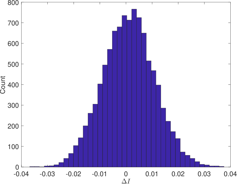
This statement is adopted and validated by real data in many works [23, 24, 25], where the authors computed the mutual information between current injections to justify the independence. The empirical histogram in Fig. 2 also suggests that $|\Delta I|$ roughly follows a Gaussian distribution. With the assumption in (3), we present the distribution analysis of $\Delta\mathbf{V}_{\mathcal{G}}$, which is key to identifying the line outage.

Suppose the outage occurs at time $\lambda$, Theorem 1 allows us to write the sequence of voltage increments as

where $g$ denotes the pre-outage Gaussian distribution and $f$ denotes the post-outage Gaussian distribution. The mean vectors $\boldsymbol{\mu}_{0},\boldsymbol{\mu}_{1}$, along with covariance matrices $\boldsymbol{\Sigma}_{0},\boldsymbol{\Sigma}_{1}$, are the parameters of these distributions. In our work, the pre-outage parameters $\boldsymbol{\mu}_{0}$ and $\boldsymbol{\Sigma}_{0}$ can be estimated using historical data during normal operation periods of the distribution grid [3]. The post-outage parameters $\boldsymbol{\mu}_{1}$ and $\boldsymbol{\Sigma}_{1}$ are considered unknown to reflect real-world outage scenarios, since the outage pattern is unpredictable/unknown. To visualize the varying distribution of the sequence, we provide an illustration of $|\Delta v[N]|\in\mathcal{R}$ in Fig. 1(b).

Before proposing our novel solution to unknown outage pattern, we present the commonly used framework to find the outage time $\lambda$ and outage branch, given voltage data in (5).

To identify the outage time $\lambda$, we conduct a sequential hypothesis test $\mathcal{H}_{0}:\lambda>N$ and $\mathcal{H}_{1}:\lambda\leq N$ at every time step $N$. As $N$ increases, the first time we reject the null hypothesis $\mathcal{H}_{0}$ determines the value of $\lambda$. To decide when to reject $\mathcal{H}_{0}$, we compute the posterior probability ratio at each time step $N$ as

where $\lambda\in\mathbb{N}$ is assumed to follow a prior distribution $\pi$. The posterior probability ratio in (III-B) compares the probabilities of “outage occurred ($\lambda\leq N$)” and “outage did not occur ($\lambda>N$)” based on the historical measurements $\Delta\mathbf{v}^{1:N}$. A larger posterior probability ratio indicates that “outage occurred” is more likely than “outage did not occur.” Therefore, we declare the outage when the ratio (III-B) exceeds a predefined threshold. By the Shiryaev-Roberts-Pollaks procedure [12, 16], the following threshold in Theorem 2 optimally considers the trade-off between the false alarm and the detection delay.

One notable feature of the detection procedure described above is its ability to function effectively without requiring knowledge of the grid topology. Additionally, it can handle non-Gaussian distributions for $f$ and $g$. As depicted in Fig. 1(c), we calculate the posterior probability ratio sequentially and identify the outage time when the ratio exceeds the threshold.

Once the line outage occurrence is detected, localizing the out-of-service branch is also critical for system recovery. In [3], the authors proposed an accurate outage localization method by proving that the voltage increments of two disconnected buses are conditionally independent. They computed the conditional correlation of every possible pair of buses in the grid and checked if the value changes from non-zero to zero. This approach differs from the utilization of nodal electric circuit matrices [26, 27] for estimating fault location, while our approach has also been effective (as shown in Section VI-D) and capitalizes on the learned covariance matrix in scenarios where the post-outage distribution is unknown.

To estimate the conditional correlation between bus $i$ and bus $k$, the covariance matrix $\boldsymbol{\Sigma}$ is utilized. Let set $\mathcal{I}:=\{i,k\}$ and $\mathcal{K}:=\mathcal{G}\backslash\{i,k\}$, the covariance matrix is decomposed as $\boldsymbol{\Sigma}=\left[\begin{matrix}\boldsymbol{\Sigma}_{\mathcal{I}\mathcal{I}}&\boldsymbol{\Sigma}_{\mathcal{I}\mathcal{K}}\\ \boldsymbol{\Sigma}_{\mathcal{I}\mathcal{K}}^{\top}&\boldsymbol{\Sigma}_{\mathcal{K}\mathcal{K}}\end{matrix}\right]$. Based on this, the conditional correlation $\rho_{ik}$ between bus $i$ and bus $k$ is

where the conditional covariance is computed by the Schur complement [28] as $\boldsymbol{\Sigma}_{\mathcal{I}|\mathcal{K}}=\boldsymbol{\Sigma}_{\mathcal{I}\mathcal{I}}-\boldsymbol{\Sigma}_{\mathcal{I}\mathcal{K}}\boldsymbol{\Sigma}_{\mathcal{K}\mathcal{K}}^{-1}\boldsymbol{\Sigma}_{\mathcal{I}\mathcal{K}}^{\top}$.

According to Theorem 3, we track the change of covariance matrices to localize the out-of-service branch. Specifically, an out-of-service branch between bus $i$ and bus $k$ can be identified if both of the following conditions are met simultaneously: (1) $|\rho_{ik}^{-}|>\delta_{\max}$ indicating the presence of a branch between buses $i$ and $k$ before the outage, and (2) $|\rho_{ik}^{+}|<\delta_{\min}$ indicating the absence of a branch between buses $i$ and $k$ after the outage. Notably, this process still does not need the grid topology as a prior.

To guarantee that the estimation of parameters $\boldsymbol{\theta}=\{\boldsymbol{\mu}_{1},\boldsymbol{\Sigma}_{1}\}$ are always feasible, we introduce the Bregman divergence [21] to constrain the estimate in each iteration of GD and arrive at a series of optimization problems as

In the above equation, $\boldsymbol{\theta}_{i}^{(e)}$ is the update of the $i^{th}$ parameter at $e^{th}$ iteration, $\boldsymbol{\theta}_{-i}^{(e)}=\boldsymbol{\theta}^{(e)}\setminus\boldsymbol{\theta}_{i}^{(e)}$ is a complement set, and $\eta$ is the trade-off learning rate. The Bregman divergence

provides a distance measurement between two variables $\boldsymbol{\theta}_{i}$ and $\boldsymbol{\theta}_{i}^{(e)}$, where $\Phi$ is a strictly convex differentiable function. Intuitively, it restricts the new estimate $\boldsymbol{\theta}_{i}^{(e+1)}$ to stay relatively close to the previous estimate $\boldsymbol{\theta}_{i}^{(e)}$. Therefore, if the initial guess $\boldsymbol{\theta}_{i}^{(0)}$ is within the feasible domain, we can expect that the parameter $\boldsymbol{\theta}_{i}$ following (13) will update towards the direction of minimizing the negative likelihood and meanwhile satisfy a similar property (e.g., positive definiteness of covariance matrix) since the update step is restricted.

Finding the solution to (13) relies on one characteristic of Bregman divergence: its gradient with respect to $\boldsymbol{\theta}_{i}$ has a simple form $\nabla_{\boldsymbol{\theta}_{i}}\Delta_{\Phi}(\boldsymbol{\theta}_{i},\boldsymbol{\theta}_{i}^{(e)})=\dot{\Phi}(\boldsymbol{\theta}_{i})-\dot{\Phi}(\boldsymbol{\theta}_{i}^{(e)}),$ where $\dot{\Phi}$ is the differential of $\Phi$. Based on this, we can eliminate the argmin in (13) by setting the gradient (with respect to $\boldsymbol{\theta}_{i}$) of the objective function to zero, and derive the following Projected Gradient Descent solution [29].

With Lemma 2, we propose the important result of our paper: the learning scheme of unknown parameters with feasibility guarantee. We will further show that this learning scheme is accurate and has convergence guarantees.

The learning process of $\boldsymbol{\Sigma}_{1}$ is shown in Fig. 3. Since matrix exponential maps any symmetric matrix to a positive definite matrix, the learning scheme (16) maintains the property of positive definiteness, i.e., $\boldsymbol{\Sigma}_{1}^{(e+1)}\succ 0$ if $\boldsymbol{\Sigma}_{1}^{(e)}\succ 0$.

Besides the statistical properties (e.g., the covariance matrix is positive definite), smart meter data have physical properties as well due to grid operation. For example, because the standard range of voltage magnitude is between $0\ p.u.$ and $1.1\ p.u.$, the mean value of voltage increment should be between $-1.1\ p.u.$ and $1.1\ p.u.$. Our learning scheme in (14) can also satisfy this requirement by defining

where $\mu_{i}$ is the $i^{th}$ element of the mean vector $\boldsymbol{\mu}_{1}$.

To conclude, when post-outage distribution parameters $\boldsymbol{\mu}_{1},\boldsymbol{\Sigma}_{1}$ are unknown, we use (17) and (16) to accurately learn them with feasibility and convergence guarantees. The pre-outage parameters $\boldsymbol{\mu}_{0}$ and $\boldsymbol{\Sigma}_{0}$ can be estimated using historical data during normal operation periods of the distribution grid [3]. By obtaining these parameters of the Gaussian density functions $g$ and $f$ in (III-B), we can explicitly calculate $g$ and $f$. It enables us to implement Theorem 2 for detecting the outage time and use Theorem 3 for localizing the outage branch. This framework is summarized into Algorithm 1.

While the non-convexity of likelihood $L(\boldsymbol{\mu}_{1},\boldsymbol{\Sigma}_{1})$ in (12) hinders us from deriving a convergence analysis directly, we note that $L(\boldsymbol{\mu}_{1},\boldsymbol{\Sigma}_{1})$ is constrained convex. Specifically, we notice that the unknown parameters $\boldsymbol{\mu}_{1},\boldsymbol{\Sigma}_{1}$ of $f$ are not supposed to be far away from the known parameters $\boldsymbol{\mu}_{0},\boldsymbol{\Sigma}_{0}$ of $g$, thus freeing us from searching the entire parameter space. This is because the alternative power supply makes the impact of line outage less severe. In fact, if $\boldsymbol{\mu}_{1},\boldsymbol{\Sigma}_{1}$ are significantly far from $\boldsymbol{\mu}_{0},\boldsymbol{\Sigma}_{0}$, distinguishing between $f$ and $g$ would become trivial: imaging a large leap from pre-outage data to post-outage data in Fig. 1(b), one can detect this change very easily. Hence, a reasonable assumption is that $\boldsymbol{\mu}_{1},\boldsymbol{\Sigma}_{1}$ are relatively close to $\boldsymbol{\mu}_{0},\boldsymbol{\Sigma}_{0}$, which actually results in a much harder detection problem. With this assumption, we can restrict our search for parameters in a constrained set where $L(\boldsymbol{\mu}_{1},\boldsymbol{\Sigma}_{1})$ has good properties. To formally present this, we introduce the restricted convexity [30].

Then, we show that $L(\boldsymbol{\mu}_{1},\boldsymbol{\Sigma}_{1})$ satisfies the restricted convexity in Definition 1. Specifically, $L(\boldsymbol{\mu}_{1})$ is restricted convex on constrained set $\left\{\boldsymbol{\mu}_{1}\left|\boldsymbol{\Sigma}_{1}\succeq\frac{\boldsymbol{v}_{k}(\boldsymbol{\mu}_{1})\boldsymbol{v}_{k}(\boldsymbol{\mu}_{1})^{T}}{(N-k+1)},\forall k\leq N\right.\right\}$ where $\boldsymbol{v}_{k}(\boldsymbol{\mu}_{1})=\sum_{n=k}^{N}(\Delta\mathbf{v}[n]-\boldsymbol{\mu}_{1})$. Similarly, $L(\boldsymbol{\Sigma}_{1})$ is restricted convex on constrained set $\{\boldsymbol{\Sigma}_{1}\succ 0|\nabla^{2}L({\rm vec}(\boldsymbol{\Sigma}_{1}))\succeq 0\}$. Based on this property, we derive in Theorem 5 the convergence of updating $\boldsymbol{\mu}_{1}$ and $\boldsymbol{\Sigma}_{1}$.

The proof is in Appendix B. Moreover, since the best update converges faster as shown in Section VI, we choose it as the output of the learning scheme in Algorithm 1. To better visualize how the parameters are updated in the restricted convex area via Projected Gradient Descent (PGD), we provide Fig. 4. As we see, although the likelihood function $L$ is not convex in the entire parameter space, the restricted area is convex, opening the door for learning accurate and feasible parameter solutions to (11).

Theorem 5 shows that our proposed method can find the optimal parameters with polynomial-time complexity, which enables quick operation. In this subsection, we provide an efficient implementation of the learning scheme to further accelerate the algorithm for timely outage identification. To achieve so, we notice that while the matrix exponential and logarithm operations in (16) provide good properties of covariance estimation, it is very time-consuming when calculating them. The calculation is time-consuming because it is often based on their infinite Taylor series. To accelerate these operations, we propose to use finite terms of their Taylor series to approximate the operations.

The matrix exponential is given by the power series in (18), and can be approximated by its first $K_{\text{exp}}$ terms since $\frac{1}{k!}$ decreases drastically when $k$ becomes large. However, once we replace the original matrix exponential operation with the approximated operation $\widehat{\exp}$, we need to verify that $\widehat{\exp}$ also maps any symmetric matrix to a positive definite matrix to satisfy the conclusion in Theorem 4. Otherwise, we will arrive at covariance estimates outside the feasible domain. With this motivation, we show in Lemma 3 that if we choose an appropriate value of $K_{\text{exp}}$ for approximation, the operation $\widehat{\exp}$ has similar properties as $\exp$.

Similarly, the matrix logarithm is given by the power series in (19), and can be approximated by the first $K_{\text{log}}$ terms.

In order to make Theorem 4 still hold true when we use the approximated operation $\widehat{\log}$, we only need the symmetry of $\widehat{\log}$, which can be easily verified as $\widehat{\log}(\boldsymbol{X}^{\top})={\textstyle\sum}_{k=1}^{K_{\text{log}}}\frac{1}{k}(-1)^{k+1}\left((\boldsymbol{X}-\boldsymbol{I})^{k}\right)^{\top}=\left(\widehat{\log}(\boldsymbol{X})\right)^{\top}.$

In summary, the proposed two approximation operations $\widehat{\exp}$ and $\widehat{\log}$ can still preserve the feasibility of the covariance matrix estimation. The choice of $K_{\text{exp}}$ and $K_{\text{log}}$ is a trade-off between execution time and approximation accuracy: when $K_{\text{exp}}$ is small, the operation $\widehat{\exp}$ is very fast but provides a poor approximation of $\exp$ and vice versa. In Section VI, we will demonstrate how we choose an appropriate approximation level which results in almost zero errors and over $75\%$ reduction in execution time.

Prior to demonstrating the accurate identification of outages with unknown post-outage distribution parameters, we must first verify that our method can learn the optimal parameters with a guaranteed convergence. Throughout the parameter learning iterations, we plot the Euclidean distance between the best update and the ground truth in Fig. 5. The plot indicates that our learning process converges to the ground truth, thereby verifying the convergence conclusion stated in Theorem 5.

After evaluating the effectiveness of using PGD to learn the unknown parameters, we then verify the performance of outage detection using such learned parameters.

The first criterion to evaluate our detection procedure is the average detection delay. To validate the asymptotic optimality of the detection delay in Theorem 2, in Fig. 6, we plot the average delay $\mathbb{E}(\tau-\lambda|\tau\geq\lambda)$ divided by $|\log\alpha|$ and the theoretical lower bound $-\log(1-\rho)+D_{KL}(f||g)$. We observe that the average detection delay of the case when $f$ is known and that of the PGD both achieve the optimal lower bound asymptotically, while the delay of PGD is slightly higher. Moreover, using PGD and accelerated PGD to learn the unknown post-outage distribution statistics enables quicker line outage detection compared to the method of MLE.

The detection rule in Theorem 2 can also restrict the false alarm rate below maximum tolerance $\alpha$. To verify this, we calculate the empirical false alarm rate $\mathbb{P}(\tau<\lambda)$ and compare it against the upper bound $\alpha$, as shown in Fig. 7. Our proposed method has similar performance compared to the case when $f$ is known since the empirical false alarm is mainly below the upper bound $\alpha$ (especially when $\alpha\to 0$). This observation demonstrates that our proposed algorithm could quickly detect line outages with a low false alarm rate, even when the post-outage distribution statistics are unknown.

In Table II, we present a summary of our proposed method’s performance in various grid systems under different outage configurations. Our method demonstrates the ability to handle diverse outage scenarios in both mesh and radial networks with DERs penetration. Specifically, when $f$ is unknown, our method exhibits a lower detection delay and significantly lower false alarm rate in comparison to MLE. Even when $f$ is given, our proposed method only experiences a slight degradation compared to the benchmark. Furthermore, Table II reveals two additional phenomena. First, when multiple branches are out-of-service simultaneously, the average detection delay is shorter than in a single-line outage scenario due to the larger KL distance between distributions $g$ and $f$ when multiple lines are disconnected. Second, in the radial network with more simulated DERs, it takes more time to detect the line outage as the KL distance between $g$ and $f$ is smaller in this case.

To compare with more relevant methods in the literature, we provide in Table III the detection performance of our proposed method and other methods. The comparison of average detection delay and false alarm rate shows that our method is only slightly degraded from the benchmark even though we have incomplete information, and outperforms other methods that also has incomplete information. The reason for this is our performance guarantee, as stated in Theorem 5, which ensures the accurate estimation of unknown post-outage distribution parameters. Furthermore, upon comparing our approach (PGD) with the machine-learning-based method (DCQ), we notice that the latter displays a greater variance in the average detection delay and false alarm rate. This can be attributed to the fact that the neural network’s parameters are randomly initialized during training, leading to a more varied estimation of the unknown post-outage distribution parameters.

In addition to detecting delay and false alarm rate, the execution time of the proposed method is also critical for timely detection. Table IV presents the execution time of Algorithm 1 on various grid systems with different sampling rates.

From the records, less than $3$ seconds per sample is needed to obtain the outage detection result when we receive a new sample, even for grid systems with more than $100$ buses. This execution time can be negligible compared to the normal smart meter sampling interval, which ranges from $1$ minute to $1$ hour. Moreover, since the most time-consuming part of our algorithm is the matrix exponential and matrix logarithm operation, we can accelerate the algorithm by approximating these operations based on their Taylor series expansion, as discussed in Section V-B.

To maintain the detection performance, we select an appropriate level of approximation with near-zero errors incurred. In Fig. 8, we choose $K_{\text{exp}}=12$ because at this approximation level, the executing time is reduced by more than $75\%$ with almost zero errors incurred. Similarly, we choose $K_{\text{log}}=16$ which is slightly larger than $K_{\text{exp}}$ since the term $\frac{1}{k}$ in (19) decreases slower than term $\frac{1}{k!}$ in (18) as $k$ becomes large. As a result, the accelerated PGD only shows a slight performance degradation, as shown in Fig. 6 and 7. More importantly, in Table IV, the acceleration technique reduces the execution time by more than half, thus achieving better timely outage detection. Evidently, the acceleration technique becomes more valuable in distribution systems with smart meters of a lower sampling rate, which is the trend of the future.

Table IV exhibits another phenomenon: as the sampling rate increases, the processing time for accumulated data $\Delta\mathbf{v}^{1:N}$ also increases. Consequently, conducting Algorithm 1 becomes challenging when $N$ grows very large. To address this issue, we discovered that a small window of historical samples can adequately differentiate between the pre- and post-outage distributions. Specifically, instead of using all $N$ samples when $N$ is very large, we can employ the latest $N_{0}$ samples to represent the entire data stream since they contain nearly identical distribution information in the temporal dimension. By doing so, the time complexity of the algorithm is restricted to a constant number, $N_{0}$. Through experiments, we determined that $N_{0}=100$ samples are sufficient to maintain the algorithm’s effectiveness and accuracy.

After detecting an outage occurrence, we further compute the conditional correlation between buses to localize the out-of-service branch, following Theorem 3. Here, Fig. 9 demonstrates the absolute conditional correlation of every pair of buses in the loopy 8-bus system before and after a line outage at branch 4-7. Since the value in the red box changes from a non-zero value before the outage ($\rho^{-}_{47}>\delta_{\max}$) to near zero after the outage ($\rho^{+}_{47}<\delta_{\min}$), we localize the out-of-service branch at 4-7, which matches the ground truth. Fig. 9(d) indicates that the localization method using the learned covariance matrix through PGD is as effective as the optimal scenario, and is more effective than using the learned covariance matrix through MLE.

Table V demonstrates the accuracy rate of localization in 1,000 experiments. As shown, our proposed method can accurately localize over 90% of the outage branches, even without the post-outage distribution parameters.

Smart-meter data can be noisy and corrupted. Besides, smart-meter data may not be accessible in every household of the distribution grid. Thus, an analysis of our proposed method under different levels of data noise and data coverage is critical to gain a better understanding of its effectiveness in real-world outage scenarios.

In the U.S., ANSI C12.20 standard permits the utility smart meters to have an error within $\pm 0.5\%$ [40]. Hence, we simulate such noise in our smart-meter voltage measurements and then evaluate the corresponding detection performance. Table VI shows both average detection delay and false alarm rate under our method with different noise levels. As we see, when the noise level is $0.5\%$, one more sample (compared to noiseless case) is needed for the detection, while the false alarm rate is also slightly increased. In fact, we are able to quantify the increase in detection delay by analyzing the change of KL divergence between the pre- and post-outage distributions affected by noisy data. In doing so, we are able to better understand and control real-world line outage detection.

Another concern regarding the smart meter data is that it may not be accessible for every household in the distribution grid, particularly in certain situations. For instance, (1) in rural areas, some households may not have installed smart meters, (2) the voltage data for certain households may be lost due to technical issues, and (3) some households may refuse to provide their voltage data due to privacy concerns. Although the new generation of smart meters is developing very fast, an analysis of incomplete coverage of smart meters data is needed to evaluate our algorithm. We first emphasize that our proposed method does not rely on the assumption of 100% coverage of smart meters data in the grid. In fact, a power line outage will influence almost all buses in the system, while the degree of influence depends on the distance between a bus and the source of the outage. Hence, we can reveal the outage by detecting the distribution change of some (not necessarily all) voltage data collected nearby the outage source.

According to [41], over 107 million smart meters were deployed by 2021, covering 75% of U.S. households. Hence, we simulate this scenario where only a ratio of buses is randomly selected to provide its voltage measurements in the grid system to detect the outage. Fig. 10 demonstrates both the average detection delay and the false alarm rate of our method under different levels of coverage ratio. In comparison to the scenario where voltage data is available for all buses, the detection delay increases by 1.2 units of time step. This means that an extra 1.2 samples of data are needed to detect the outage in the 75% data coverage scenario. Similarly, when the data coverage ratio drops to 50%, an additional 6.9 samples are required for detection. Furthermore, as the data coverage ratio decreases to only 50%, the false alarm rate increases from 0.7% to 21.9%.

Our detection procedure involves certain hyper-parameters that have the potential to influence the detection performance, such as the geometric distribution parameter $\rho$. Therefore, conducting a sensitivity analysis pertaining to these hyper-parameters is crucial to assess the robustness of our proposed method.

During our experiments, we randomly simulated the outage time $\lambda$ using a geometric prior distribution denoted as $\text{Geo}(\rho)$. This distribution aligns with our assumption that outages can take place in any time step with an equal probability of $\rho$. Fig. 11 illustrates the effect of the parameter $\rho$ on the performance of our detection method. It can be observed that choosing different values of $\rho$ within the range of $0.004$ to $0.05$ has a negligible impact on both the false alarm rate (approximately 1.65%) and the localization accuracy (approximately 92.8%). Additionally, decreasing the value of $\rho$ leads to a slight increase in the average detection delay.

References

- [1] A. N. Samudrala, M. H. Amini, S. Kar, and R. S. Blum, “Distributed outage detection in power distribution networks,” IEEE Transactions on Smart Grid, vol. 11, no. 6, pp. 5124–5137, 2020.
- [2] Energy Information Administration, “Average frequency and duration of electric distribution outages vary by states,” https://www.eia.gov/todayinenergy/detail.php?id=35652, Accessed Sep. 2022.
- [3] Y. Liao, Y. Weng, C.-W. Tan, and R. Rajagopal, “Quick line outage identification in urban distribution grids via smart meters,” CSEE Journal of Power and Energy Systems, 2021.
- [4] D. Bakken, Smart grids: clouds, communications, open source, and automation. CRC Press, 2014.
- [5] A. Meier, T. Ueno, and M. Pritoni, “Using data from connected thermostats to track large power outages in the united states,” Applied Energy, vol. 256, p. 113940, 2019.
- [6] M. He and J. Zhang, “Fault detection and localization in smart grid: A probabilistic dependence graph approach,” in IEEE International Conference on Smart Grid Communications, 2010, pp. 43–48.
- [7] M. Babakmehr, F. Harirchi, A. Al-Durra, S. Muyeen, and M. G. Simões, “Compressive system identification for multiple line outage detection in smart grids,” IEEE Transactions on Industry Applications, 2019.
- [8] R. A. Sevlian, Y. Zhao, R. Rajagopal, A. Goldsmith, and H. V. Poor, “Outage detection using load and line flow measurements in power distribution systems,” IEEE Transactions on Power Systems, 2017.
- [9] H. Sun, Z. Wang, J. Wang, Z. Huang, N. Carrington, and J. Liao, “Data-driven power outage detection by social sensors,” IEEE Transactions on Smart Grid, vol. 7, no. 5, pp. 2516–2524, 2016.
- [10] P. Kankanala, S. Das, and A. Pahwa, “Adaboost: An ensemble learning approach for estimating weather-related outages in distribution systems,” IEEE Transactions on Power Systems, vol. 29, no. 1, pp. 359–367, 2013.
- [11] A. Dwivedi and A. Tajer, “Scalable quickest line outage detection and localization via graph spectral analysis,” IEEE Transactions on Power Systems, vol. 37, no. 1, pp. 590–602, 2021.
- [12] A. N. Shiryaev, “On optimum methods in quickest detection problems,” Theory of Probability & Its Applications, vol. 8, no. 1, pp. 22–46, 1963.
- [13] C. Wei, A. Wiesel, and R. S. Blum, “Change detection in smart grids using errors in variables models,” in IEEE Sensor Array and Multichannel Signal Processing Workshop, 2012, pp. 17–20.
- [14] Y. C. Chen, T. Banerjee, A. D. Domínguez-García, and V. V. Veeravalli, “Quickest line outage detection and identification,” IEEE Transactions on Power Systems, vol. 31, no. 1, pp. 749–758, 2016.
- [15] K. Gajula, V. Le, X. Yao, S. Zou, and L. Herrera, “Quickest detection of series arc faults on dc microgrids,” in IEEE Energy Conversion Congress and Exposition, 2021, pp. 796–801.
- [16] A. G. Tartakovsky and V. V. Veeravalli, “General asymptotic bayesian theory of quickest change detection,” Theory of Probability & Its Applications, vol. 49, no. 3, pp. 458–497, 2005.
- [17] Y. Cao, L. Xie, Y. Xie, and H. Xu, “Sequential change-point detection via online convex optimization,” Entropy, vol. 20, no. 2, p. 108, 2018.
- [18] D. Siegmund and E. Venkatraman, “Using the generalized likelihood ratio statistic for sequential detection of a change-point,” The Annals of Statistics, pp. 255–271, 1995.
- [19] S. B. Fotopoulos, V. K. Jandhyala, and E. Khapalova, “Exact asymptotic distribution of change-point mle for change in the mean of gaussian sequences,” The Annals of Applied Statistics, 2010.
- [20] N. Duan, C. Huang, C.-C. Sun, and L. Min, “Smart meters enabling voltage monitoring and control: The last-mile voltage stability issue,” IEEE Transactions on Industrial Informatics, 2021.
- [21] L. M. Bregman, “Finding the common point of convex sets by the method of successive projection,” in Doklady Akademii Nauk, vol. 162, no. 3. Russian Academy of Sciences, 1965, pp. 487–490.
- [22] A. M. Kettner and M. Paolone, “On the properties of the power systems nodal admittance matrix,” IEEE Transactions on Power Systems, vol. 33, no. 1, pp. 1130–1131, 2017.
- [23] D. Deka, S. Backhaus, and M. Chertkov, “Structure learning in power distribution networks,” IEEE Transactions on Control of Network Systems, vol. 5, no. 3, pp. 1061–1074, 2017.
- [24] S. Bolognani, N. Bof, D. Michelotti, R. Muraro, and L. Schenato, “Identification of power distribution network topology via voltage correlation analysis,” in IEEE Conference on Decision and Control, 2013.
- [25] Y. Liao, Y. Weng, G. Liu, and R. Rajagopal, “Urban mv and lv distribution grid topology estimation via group lasso,” IEEE Transactions on Power Systems, vol. 34, no. 1, pp. 12–27, 2018.
- [26] S. Jamali, A. Bahmanyar, and E. Bompard, “Fault location method for distribution networks using smart meters,” Measurement, vol. 102, pp. 150–157, 2017.
- [27] S. S. Gururajapathy, H. Mokhlis, and H. A. Illias, “Fault location and detection techniques in power distribution systems with distributed generation: A review,” Renewable and sustainable energy reviews, vol. 74, pp. 949–958, 2017.
- [28] S. Boyd, S. P. Boyd, and L. Vandenberghe, Convex optimization. Cambridge university press, 2004.
- [29] K. Tsuda, G. Rätsch, and M. K. Warmuth, “Matrix exponential gradient updates for on-line learning and bregman projection,” in Advances in Neural Information Processing Systems, 2004, pp. 1425–1432.
- [30] P. Jain and P. Kar, “Non-convex optimization for machine learning,” arXiv preprint arXiv:1712.07897, 2017.
- [31] W. H. Kersting, “Radial distribution test feeders,” IEEE Transactions on Power Systems, vol. 6, no. 3, pp. 975–985, 1991.
- [32] C. Mateo, G. Prettico, T. Gómez, R. Cossent, F. Gangale, P. Frías, and G. Fulli, “European representative electricity distribution networks,” International Journal of Electrical Power & Energy Systems, 2018.
- [33] A. P. Dobos, “Pvwatts version 5 manual,” National Renewable Energy Lab.(NREL), Golden, CO (United States), Tech. Rep., 2014.
- [34] Y. Liao, A. S. Kiremidjian, R. Rajagopal, and C.-H. Loh, “Structural damage detection and localization with unknown postdamage feature distribution using sequential change-point detection method,” Journal of Aerospace Engineering, vol. 32, no. 2, p. 04018149, 2019.
- [35] Y. C. Chen, T. Banerjee, A. D. Dominguez-Garcia, and V. V. Veeravalli, “Quickest line outage detection and identification,” IEEE Transactions on Power Systems, vol. 31, no. 1, pp. 749–758, 2015.
- [36] G. Rovatsos, X. Jiang, A. D. Domínguez-García, and V. V. Veeravalli, “Comparison of statistical algorithms for power system line outage detection,” in 2016 IEEE international conference on acoustics, speech and signal processing (ICASSP). IEEE, 2016, pp. 2946–2950.
- [37] T. S. Lau, W. P. Tay, and V. V. Veeravalli, “Quickest change detection with unknown post-change distribution,” in 2017 IEEE International Conference on Acoustics, Speech and Signal Processing (ICASSP). IEEE, 2017, pp. 3924–3928.
- [38] J. Z. Hare, L. Kaplan, and V. V. Veeravalli, “Toward uncertainty aware quickest change detection,” in 2021 IEEE 24th International Conference on Information Fusion (FUSION). IEEE, 2021, pp. 1–8.
- [39] X. Ma, L. Lai, and S. Cui, “A deep q-network based approach for online bayesian change point detection,” in 2021 IEEE 31st International Workshop on Machine Learning for Signal Processing (MLSP). IEEE, 2021, pp. 1–6.
- [40] J. Zheng, D. W. Gao, and L. Lin, “Smart meters in smart grid: An overview,” in IEEE Green Technologies Conference, 2013, pp. 57–64.
- [41] Institution for Electronic Innovation, “Electric company smart meter deployments: Foundation for a smart grid,” https://www.edisonfoundation.net/-/media/Files/IEI/publications/IEI_Smart_Meter_Report_April_2021.ashx, Accessed Sep. 2022.
- [42] R. B. Bapat, Graphs and matrices. Springer, 2010, vol. 27.