Ab initio transport calculations: from normal to superconducting current

H. Ness Affiliation: Department of Physics, King’s College London, Strand, London WC2R 2LS, UK M. van Schilfgaarde Affiliation: Department of Physics, King’s College London, Strand, London WC2R 2LS, UK Affiliation: National Renewable Energy Laboratory, Golden, Colorado 80401, USA

Abstract

Applying the Bogoliubov-de Gennes equations with density-functional theory, it is possible to formulate first-principles description of current-phase relationships in superconducting/normal (magnetic)/superconducting trilayers. Such structures are the basis for the superconducting analog of Magnetoresistive random access memory devices (JMRAM). In a recent paper [Ness et al. 2022] we presented results from the first attempt to formulate such a theory, applied to the Nb/Ni/Nb trilayers. In the present work we provide computational details, explaining how to construct key ingredient (scattering matrices $S_{N}$ ) in a framework of linear muffin-tin orbitals (LMTO).

I Introduction

In a recent paper [Ness et al. 2022], we have combined density functional theory and the Bogoliubov-de Gennes equations to form a first-principles approach to the study of transport in magnetic Josephson junctions (MJJ). This method allowed us to predict and explain the properties of realistic MJJs such as the period of oscillation and decay of the critical current oscillations with the ferromagnet thickness. We applied our methodology to study realistic material stacks of the Nb/Ni/Nb trilayer and established that suppression of supercurrent is an intrinsic property of the junctions, even in absence of disorder.

To determine the supercurrent in a superconductor–normal metal–superconductor (S/N/S) junction from a density-functional approach (which is inherently single-particle), one needs to “decompose” the entire scattering process into different steps. First we use the Andreev approximation to account for electron–hole scattering processes Beenakker 1992, the (spin-resolved) Andreev reﬂection at each left S/N and right N/S interfaces is described by a reflection matrix. Second, we assume that the main contribution to the supercurrent comes from Andreev bound states localized in the junction (in the short junction limit) in the energy window corresponding to the superconducting gap. The energy spectrum of the Andreev bound states can be obtained by solving an equation Beenakker 1992; Beenakker 2004; van Heck et al. 2014; de Jong and Beenakker 1995 which basically states the conservation of incoming/outgoing particle fluxes following scattering in the normal state region and Andreev reflections at the left S/N and right N/S interfaces. This equation involves the Andreev reflection matrices (at the left S/N and right N/S interfaces) as well as the scattering matrices $S_{N}$ for electron- and $S_{N}^{*}$ hole-like waves in the central normal N region. These single-particle (normal state) $S_{N}$ scattering matrices are needed the objects we obtain from density-functional theory.

In the present paper, we show in detail how to obtain such scattering matrices from the Questaal suite, which is an open access electronic structure code based on the LMTO technique Que; Pashov et al. 2020.

II Transport in the normal state

The Questaal package Que; Pashov et al. 2020 calculates the single-particle electronic structure and includes some many-body effect corrections as well. It is based on the LMTO technique.

One of Questaal’s packages provides the ability to calculates the full non-equilibrium (NE) transport properties of an infinite $L$ - $C$ - $R$ system representing a central region $C$ cladded by two semi-infinite $L$ and $R$ leads Faleev et al. 2005. The transport properties are obtained by using the NE Green’s functions (GF) formalism Meir and Wingreen 1992. The transport calculations are done with a LMTO basis-set in the so-called Atomic Sphere Approximation. Owing to the finite range of the basis set, the $L$ - $C$ - $R$ system can be described in terms of an infinite stack of principal-layers (PLs) which interact only with their nearest neighboring PLs (Fig. 1). The direction of the electronic current is perpendicular to the PLs, and periodic boundary conditions are used within each PL. The discretization of the surface Brillouin zone of the corresponding PL introduces a set of transverse momentum $k_{\parallel}$ . Before transport calculations are performed, the density of the $L$ - $C$ - $R$ must be computed self-consistently in a standard DFT framework. Apart from a constant shift, potentials in the semi-infinite $L$ - and $R$ - layers are kept frozen at the potential of their respective bulk systems. A dipole must form across the $C$ region so that the $L$ - and $R$ - Fermi levels align. This is generated in the course of the self-consistent cycle, and also determines the shift needed to align the $L$ - and $R$ - Fermi levels. The first account of this method was presented in Ref.[van Schilfgaarde and Lambrecht 1998], and the formalism is described in detail in Ref.[Faleev et al. 2005], including its implementation for the non-equilibrium cases. Self-consistency can be obtained in the non-equilibrium case, though it is not important here.

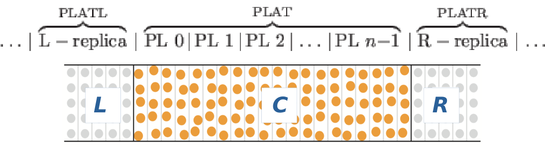
Refer to caption — Figure 1: Schematic representation of the stacking of principal-layers PLs for the calculation of the transport in two-terminal $L$ - $C$ - $R$ junctions.

The key quantity is the total transmission probability $T(E,V)$ from which the non-linear current can be obtained with the conventional Landauer-like elastic scattering framework. The linear conductance regime is simply described by $T(E_{F},V=0)$ taken at the Fermi energy $E_{F}$ of the $L$ - $C$ - $R$ system at equilibrium. The total transmission probability $T(E,V)$ is given by

T(E,V)=\sum_{k_{\parallel},\sigma}w_{k_{\parallel}}T(E,V;k_{\parallel},\sigma)\ ,

(1)

where $w_{k_{\parallel}}$ is the weight associated with the transverse momentum $k_{\parallel}$ , and $\sigma$ is the spin of the electron.

The partial transmission probability $T(E,V;k_{\parallel},\sigma)$ are obtained from NEGF Meir and Wingreen 1992 as follows:

\begin{split}&T(E,V;k_{\parallel},\sigma)=\\ &{\rm Tr}_{C}\left[\Gamma_{LL}(E;k_{\parallel})\ G^{r}_{LR}(E;k_{\parallel})\ \Gamma_{RR}(E;k_{\parallel})\ G^{a}_{RL}(E;k_{\parallel})\right]\ ,\end{split}

(2)

where (for simplifying the notation, explicit dependence of spin $\sigma$ and bias $V$ has been dropped) the trace is taken over the basis set of the central $C$ region. The GF $G^{r/a}$ are the retarded/advanced NEGF of the $C$ region connected to the leads, i.e. $G^{r/a}=[g^{r/a}-\Sigma^{r/a}_{LL}-\Sigma^{r/a}_{RR}]^{-1}$ , where $\Sigma^{r/a}_{LL}$ and $\Sigma^{r/a}_{RR}$ are the corresponding $L$ and $R$ lead self-energies respectively ( $g^{r/a}$ is the GF of the disconnected $C$ region). The quantities $\Gamma_{LL/RR}$ are the imaginary part of the lead self-energies, $\Gamma_{LL/RR}={\rm i}(\Sigma^{r}-\Sigma^{a})_{LL/RR}$ . Finally, $G_{LR}$ are the NEGF matrix elements connecting the most-left PL of the $C$ region to the most-right PL of region $C$ .

In order to calculate the supercurrent in the junctions, we actually need the full scattering matrix $S_{N}$ of the central region. The $S_{N}$ matrix is built from the transmission (reflection) coefficients between the $L$ and $R$ and not from the transmission (reflection) probability Eq. (2). This marks one essential difference between describing superconducting and normal transport: $S_{N}$ has additional information not needed for transmission in the normal state.

Hence, we need to apply a transformation to Eq.(2) to be able to extract the transmission coefficients. Instead of folding down the degrees of freedom of the $L$ and $R$ leads into a closed form for the lead self-energies and calculating the transmission probability from a trace over the degrees of freedom of the central $C$ region, we have to unfold these degrees of freedom and calculate the transmission probability from a trace over the these degrees of freedom. The latter can form propagating waves in the $L$ and $R$ leads which are linked by transmission and reflection coefficients as in the original picture of Landauer-like scattering Fisher and Lee 1981.

Therefore we first need to determine the eigenmodes of propagation in the $L$ and $R$ leads, and then transform the lead self-energies into the eigenmode basis of these propagating states.

II.1 Eigenmodes of propagation in the leads

II.1.1 Bulk GF

Deep inside the leads, one can calculate the eigenmodes of propagation by solving a nearest-neighbor (in terms of PLs) tight-binding-like equation for the bulk GF $g_{p,p^{\prime}}$

-S_{0,-1}g_{-1,0}+(P-S)_{0,0}g_{0,0}-S_{0,1}g_{1,0}=1\ .

(3)

In the LMTO language Pashov et al. 2020, the quantity $(P-S)_{0,0}$ plays the role of a local energy-dependent Hamiltonian in the PL (with index $p=0$ ), where $P$ are the so-called potential functions and the structure constant $S_{p,p^{\prime}}$ couples only adjacent PLs ( $p-p^{\prime}=\pm 1$ ). The bulk is translationally invariant in the direction perpendicular to the PLs; hence $S_{0,-1}=S_{1,0}$ and $g_{-1,0}=g_{0,1}$ .

One solves the equation

-S_{1,0}g_{0,1}+(P-S)_{0,0}g_{0,0}-S_{0,1}g_{1,0}=1

(4)

by expanding the wavefunction coefficients as a solution $\bm{\alpha}$ of a quadratic equation Chen et al. 1989. This quadratic equation can be recast into a generalized eigenvalue problem $\bm{A}\bm{x}=\lambda\bm{B}\bm{x}$ by introducing a new vector $\bm{\beta}=\lambda\bm{\alpha}$ and working in a enlarged (doubled) vector space Chen et al. 1989; Fujimoto and Hirose 2003. The generalized eigenvalue problem is written as:

\left[\begin{array}[]{cc}-{S}_{1,0}&(P-S)_{0,0}\\ {0}&{S}_{0,1}\end{array}\right]\left[\begin{array}[]{c}\bm{\alpha}\\ \bm{\beta}\end{array}\right]=\lambda\left[\begin{array}[]{cc}{0}&{S}_{0,1}\\ {S}_{0,1}&{0}\end{array}\right]\left[\begin{array}[]{c}\bm{\alpha}\\ \bm{\beta}\end{array}\right]\ ,

(5)

and can be solved from a set of two independent equations:

-S_{1,0}Pr^{-1}P^{-1}+(P-S)_{0,0}-S_{0,1}PrP^{-1}=0

(6)

and

-S_{1,0}Qx^{-1}Q^{-1}+(P-S)_{0,0}-S_{0,1}QxQ^{-1}=0\ .

(7)

Note that all matrices $M\equiv S,g,Q,P$ are dependent on variables $M\equiv M(E;k_{\parallel},\sigma)$ . The above equations need to be solved for each energy $E$ , each $k_{\parallel}$ and each spin $\sigma$ .

The eigenvalue vectors $r$ and $x$ characterize the propagating (or decaying) modes in the bulk. Their meaning becomes clear when written as Bloch-like factors $e^{\pm ik_{z}a}$ , where $a$ is the characteristic width of the PL and $k_{z}$ is the (energy dependent) wave number normal to the interface. The columns of the matrices $P$ and $Q$ are the corresponding eigenvectors. For the propagating modes, the wave numbers $k_{z}(E;k_{\parallel},\sigma)$ are real numbers; $k_{z}(E)$ contains a non-zero imaginary part for the decaying modes. We choose the following convention: $|r_{i}|\leq 1$ (propagating and decaying modes towards the right) and $|x_{i}|\geq 1$ (propagating and decaying modes towards the left).

II.1.2 Reformulating the generalized eigenvalue problem

One can rewrite the central equations of the previous section in term of the wavefunctions $\phi_{p}$ of the PL $p$ deep inside the leads:

-S_{1,0}\phi_{p-1}+g_{b}^{-1}\phi_{p}+S_{0,1}\phi_{p+1}=0

(8)

as the system is translation-invariant in the bulk of the leads. For notation convenience, we use $g_{b}^{-1}=(P-S)_{0,0}$ .

By introducing the ratio matrix ${R}_{p}^{\leftarrow}=\phi_{p-1}\phi_{p}^{-1}$ and by manipulation of the recursion relation

\phi_{p}=g_{b}S_{1,0}\phi_{p-1}+g_{b}S_{0,1}\phi_{+1}\ ,

(9)

one ends up with the following expression Fujimoto and Hirose 2003 for the ratio matrix ${R}_{p+1}^{\leftarrow}$ :

{R}_{p+1}^{\leftarrow}=\left({1}+g_{b}S_{1,0}[{1}-{R}_{p}^{\leftarrow}g_{b}S_{1,0}]^{-1}{R}_{p}^{\leftarrow}\right)g_{b}S_{0,1}\ .

(10)

As the bulk of the lead is translation-invariant, we can use the generalized Bloch condition $\phi_{p+1}=\lambda\phi_{p}$ between adjacent PLs (note that this is reminiscent of the relation $\bm{\beta}=\lambda\bm{\alpha}$ used in the previous section). The ratio matrix becomes ${R}_{p}^{\leftarrow}=\phi_{p-1}\phi_{p}^{-1}=\lambda^{-1}$ , and Eq. (10) is another formulation of the quadratic equation Chen et al. 1989 discussed previously.

However, we have found this expression can be used as an iterative scheme, i.e.

\lambda_{i+1}^{-1}=\left({1}+g_{b}S_{1,0}[\lambda_{i}-g_{b}S_{1,0}]^{-1}\right)g_{b}S_{0,1}

(11)

to improve (at will) the accuracy (precision) of the eigenvalues $\lambda\equiv(r,x)$ . This is particularly crucial in the cases of degenerate modes that might occur at particular $E$ and $k_{\parallel}$ .

II.1.3 The case of singular matrices

We have also implemented the possibilities of dealing with singular matrices that may occur in the generalized eigenvalue problem $\bm{A}\bm{x}=\lambda\bm{B}\bm{x}$ which is not easily solvable when one, or both, $\bm{A},\bm{B}$ are singular. An eigenvalue shift procedure can be used to solve the linear generalized eigenvalue problem when both matrices are singular and when the full eigensystem is required A. Jennings and Cole 1978.

For that one adds the term $-\alpha\bm{B}\bm{x}$ on both sides of $\bm{A}\bm{x}=\lambda\bm{B}\bm{x}$ . If $\bar{\bm{A}}=\bm{A}-\alpha\bm{B}$ is not singular, one can calculate $\bar{\bm{M}}=\bar{\bm{A}}^{-1}\bm{B}$ and solve the conventional eigenvalue problem:

\bar{\bm{M}}\bm{x}=\frac{1}{\lambda-\alpha}\bm{x}.

(12)

A typical eigenvalue $\gamma$ of $\bar{\bm{M}}$ must be related to one of the $\lambda$ values according to $\gamma=1/\mu$ where $\mu=\lambda-\alpha$ , with the corresponding eigenvector unchanged.

II.2 Surface Green’s functions

We can now build the surface GF of the leads which enters into the definition of the lead self-energies $\Sigma^{r/a}_{RR}$ . The $L$ and $R$ surface GFs are obtained from only one part of the eigenmodes, i.e. from the propagating modes and the modes that decay inside the bulk of the corresponding lead Chen et al. 1989.

The surface GF of the $R$ lead is obtained from

g_{RR}=\left[g_{b}^{-1}-S_{0R}PrP^{-1}\right]^{-1}

(13)

and the $L$ lead surface GF from

g_{LL}=\left[g_{b}^{-1}-S_{0L}Qx^{-1}Q^{-1}\right]^{-1}\ .

(14)

We have used an explicit notation for the leads’ structure constant, $S_{0R}$ and $S_{0L}$ , as the two $L$ and $R$ leads need not be identical.

In comparison to the bulk case in Sec. II.1.1, we have $S_{0R}=S_{0,1}$ and $S_{R0}=S_{1,0}$ for the $R$ region, and $S_{0L}=S_{1,0}$ and $S_{L0}=S_{0,1}$ for the $L$ region. Note the different ordering of the subscript of the bulk structure constant for the $L$ and $R$ regions: the $R$ ( $L$ ) surface GF is built from “propagating” towards two different $R$ ( $L$ ) directions.

By introducing Eq. (6) into Eq. (13), and Eq. (7) into Eq. (14), we find that the matrices $P,P^{-1}$ ( $Q,Q^{-1}$ ) are the transformations that diagonalize $g_{RR}S_{R0}$ ( $g_{LL}S_{L0}$ ) respectively. Indeed, we have

g_{RR}=\left[S_{R0}Pr^{-1}P^{-1}\right]^{-1}\ ,

(15)

or equivalently

g_{RR}S_{R0}=PrP^{-1}\ ,

(16)

and

g_{LL}S_{L0}=Qx^{-1}Q^{-1}\ .

(17)

The matrices $P,P^{-1}$ ( $Q,Q^{-1}$ ) perform the change of basis set, from the original basis to the basis of the propagation eigenmodes.

II.3 Transmission coefficients

We now proceed with the transformation of the quantities $\Gamma_{\alpha\alpha}$ into the basis of the propagation eigenmodes. The quantity $\Gamma_{\alpha\alpha}$ is related to the imaginary part of the lead self-energy $\Sigma_{\alpha\alpha}$ ( $\alpha{=}L,R$ )

\Gamma_{\alpha\alpha}=S_{0\alpha}\ {\rm i}\left[g^{r}_{\alpha\alpha}-g^{a}_{\alpha\alpha}\right]S_{\alpha 0}\ .

(18)

Using Eq. (17) and the relation $S_{0L}g^{a}_{LL}=(g^{r}_{LL}S_{L0})^{\dagger}=(Q^{-1})^{\dagger}(x^{-1})^{\dagger}Q^{\dagger}$ , we find that

\Gamma_{LL}={\rm i}\left(S_{0L}Qx^{-1}Q^{-1}-(Q^{-1})^{\dagger}(x^{-1})^{\dagger}Q^{\dagger}S_{L0}\right)\ .

(19)

Introducing the identity $1=QQ^{-1}$ ( $1=(Q^{-1})^{\dagger}Q^{\dagger}$ ) to the right (left) side of the second (first) term in Eq. (19), one ends up with:

\Gamma_{LL}=(Q^{-1})^{\dagger}v_{L}Q^{-1}

(20)

where

v_{L}={\rm i}\left[Q^{\dagger}S_{0L}Qx^{-1}-\left(Q^{\dagger}S_{0L}Qx^{-1}\right)^{\dagger}\right]\ .

(21)

Proceeding similarly for $\Gamma_{RR}$ , we get

\Gamma_{RR}=(P^{-1})^{\dagger}v_{R}P^{-1}

(22)

where

v_{R}={\rm i}\left[P^{\dagger}S_{0R}Pr-\left(P^{\dagger}S_{0R}Pr\right)^{\dagger}\right]

(23)

It is crucial to note that the matrices $v_{L}$ and $v_{R}$ correspond to the expectation values of the current operator calculated in the basis set of the eigenmodes Wimmer 2008.

For non-degenerate modes, the diagonal elements $v_{L,n}$ ( $v_{R,m}$ ) correspond to the group velocity $\partial E/\partial k$ of the propagating mode $n$ ( $m$ ) in the $L$ ( $R$ ) region Fujimoto and Hirose 2003; Wimmer 2008. For decaying modes the diagonal elements are simply zero. In the case of degeneracy, the velocity matrices $v_{L}$ and $v_{R}$ are block diagonal. Then we need to apply a further transformation to get diagonal matrices $v_{L,R}\rightarrow v^{D}_{L,R}$ Wimmer 2008.

Once the velocity matrices $v_{L}$ and $v_{R}$ are diagonal, we can write $v^{D}_{L,n}=\text{sgn}(v^{D}_{L,n})|v^{D}_{L,n}|^{1/2}|v^{D}_{L,n}|^{1/2}$ and $v^{D}_{R,m}=\text{sgn}(v^{D}_{R,m})|v^{D}_{R,m}|^{1/2}|v^{D}_{R,m}|^{1/2}$ , and transform Eq. (2) as follows:

\begin{split}&{\rm Tr}_{C}\left[\Gamma_{LL}\ G^{r}_{LR}\ \Gamma_{RR}\ G^{a}_{RL}\right]\\ &={\rm Tr}\left[(Q^{-1})^{\dagger}v^{D}_{L}Q^{-1}g^{r}_{LR}(P^{-1})^{\dagger}v^{D}_{R}P^{-1}g^{a}_{LR}\right]\\ &={\rm Tr}_{L+R}\left[\ t_{LR}\ t_{LR}^{\dagger}\ \right]\ .\end{split}

(24)

The transmission probability is now expressed in terms of transmission coefficients $t_{n,m}$ linking the propagating modes $n$ of the $L$ lead to the propagating modes $m$ of the $R$ lead. The transmission coefficients are given by a generalized Fisher-Lee expression Fisher and Lee 1981:

\begin{split}&t_{LR}\equiv\\ &t_{n,m}(E;k_{\parallel},\sigma)={\rm i}|v^{D}_{L,n}|^{1/2}\left[{Q^{-1}\ g^{r}_{LR}\ (P^{-1})^{\dagger}}\right]_{n,m}|v^{D}_{R,m}|^{1/2}\end{split}

(25)

It is important to note that the original Meir and Wingreen expression Meir and Wingreen 1992 involves a trace over the degrees of freedom in the $C$ region (first line in Eq. (24) ), while the Fisher and Lee expression Fisher and Lee 1981 involves a trace over the propagating modes in the $L$ and $R$ leads (last line in Eq. (24) ).

II.4 Reflection coefficients

In analogy to the transmission probability, we can also define reflection probabilities in the same lead:

\begin{split}R_{L}(E)&={\rm Tr}_{C}\left[\Gamma_{LL}\ G^{r}_{LL}\ \Gamma_{LL}\ G^{a}_{LL}\right]\\ R_{R}(E)&={\rm Tr}_{C}\left[\Gamma_{RR}\ G^{r}_{RR}\ \Gamma_{RR}\ G^{a}_{RR}\right]\end{split}

(26)

Following the derivations given in the previous section we find (for the $L$ region):

\begin{split}&{\rm Tr}_{C}\left[\Gamma_{LL}\ G^{r}_{LL}\ \Gamma_{LL}\ G^{a}_{LL}\right]\\ &={\rm Tr}\left[(Q^{-1})^{\dagger}v_{L}Q^{-1}g^{r}_{LL}(Q^{-1})^{\dagger}v_{L}Q^{-1}g^{a}_{LL}\right]\\ &={\rm Tr}_{L}\left[r_{LL}(r_{LL})^{\dagger}\right]\end{split}

(27)

The reflection coefficients $r_{LL}=r_{n,n^{\prime}}$ are now expressed in the basis of the propagating modes $n$ and $n^{\prime}$ of the $L$ lead.

Similarly, one can find the reflection probability $R_{R}(E)={\rm Tr}_{R}\left[r_{RR}(r_{RR})^{\dagger}\right]$ from the reflection coefficients $r_{RR}=r_{m,m^{\prime}}$ expressed in the basis of the propagating modes $m$ and $m^{\prime}$ of the $R$ lead.

One should note that the reflection probability, defined in Eq. (26), contains the contributions of both the $L$ ( $R$ ) incoming wave(s) and the reflected waves in the $L$ ( $R$ ) region. In order to obtain the correct reflection coefficients (and proper flux conservation), one needs to suppress the contribution of the incoming wave in the $n$ -th $L$ channel ( $m$ -th $R$ channel) in the $L$ ( $R$ ) lead respectively.

Hence the expressions of the reflection coefficients are as follows:

\begin{split}&r_{LL}=r_{n,n^{\prime}}(E;k_{\parallel},\sigma)=\\ &{\rm i}|v^{D}_{L,n}|^{1/2}\ \left[Q^{-1}\ g^{r}_{LL}\ (Q^{-1})^{\dagger}\right]_{n,n^{\prime}}|v^{D}_{L,n^{\prime}}|^{1/2}-\delta_{nn^{\prime}}\end{split}

(28)

and

\begin{split}&r_{RR}=r_{m,m^{\prime}}(E;k_{\parallel},\sigma)=\\ &{\rm i}|v^{D}_{R,m}|^{1/2}\ \left[P^{-1}\ g^{r}_{RR}\ (P^{-1})^{\dagger}\right]_{m,m^{\prime}}|v^{D}_{R,m^{\prime}}|^{1/2}-\delta_{mm^{\prime}}\end{split}

(29)

III Full scattering matrix and supercurrent

The full scattering matrix $S_{N}$ is built from the reflection coefficients $r_{LL}$ and $r_{LL}$ , and from the transmission coefficients $t_{LR}$ and $t_{RL}$ ( $t_{RL}$ is the transpose of $t_{LR}$ ). All quantities are explicitly dependent of $(E;k_{\parallel},\sigma)$ .

For the calculations of the supercurrent, we construct the normal state scattering matrix $S_{N}$ as follows:

	$\displaystyle S_{N}(E;k_{\parallel})=\left(\begin{array}[]{cc}\left[\begin{array}[]{cc}r_{LL}(\uparrow)&0\\ 0&r_{LL}(\downarrow)\end{array}\right]&\left[\begin{array}[]{cc}t_{LR}(\uparrow)&0\\ 0&t_{LR}(\downarrow)\end{array}\right]\\ \\ \left[\begin{array}[]{cc}t_{RL}(\uparrow)&0\\ 0&t_{RL}(\downarrow)\end{array}\right]&\left[\begin{array}[]{cc}r_{RR}(\uparrow)&0\\ 0&r_{RR}(\downarrow)\end{array}\right]\\ \end{array}\right)$
	.		(42)

The normal state scattering matrix $S_{N}(E_{F}+\varepsilon;k_{\parallel})$ characterizes electron (particle) transport for a positive energy $\varepsilon$ above the Fermi level $E_{F}$ . The transport of hole (antiparticle) is given by the time-reserved symmetric $S_{N}^{*}(E_{F}-\varepsilon;k_{\parallel})$ scattering matrix for (negative) energy $-\varepsilon$ below $E_{F}$ .

As mentioned above, the dc Josephson current in the junction is obtained from the Andreev bound states formed in the junction. The spectrum of the Andreev bound states can be calculated from a scattering matrix formalism Beenakker 1992; Beenakker 2004 In such an approach, the spatial separation of Andreev and normal scattering is the key simplification which allows one to relate the Josephson current directly to the normal-state scattering matrix of the junction.

We have successfully applied such an approach in a recent paper Ness et al. 2022 to the study of the supercurrent decay and oscillation in magnetic Josephson junctions made of Ni layers connected to two Nb leads.

IV Application

We now provide an illustrative example of our eigenmode approach applied to a simple case. We consider that all PLs in the $L$ - $C$ - $R$ junction are identical, i.e. we study the bulk (equilibrium) transport properties of a “perfect” crystal. In this case, the transmission probability (at a given energy $E$ and for a given $k_{\parallel}$ point) is simply given by the number of “real” bands crossing that energy $E$ at that $k_{\parallel}$ point, each “real” band corresponding to a propagating mode. We compare the results obtained from the two Meir and Wingreen Meir and Wingreen 1992 and Fisher and Lee Fisher and Lee 1981 expressions.

Figure 2 shows the transmission probability $T(E,V;k_{\parallel},\sigma)$ calculated at equilibrium $V{=}0$ and for spin $\uparrow$ of bulk Co. The unique PL of bulk Co is made of 2 atoms of Co with 9 (spd) orbitals, i.e. the size of the matrices corresponding to that PL is 18 $\times$ 18 per spin. The calculations performed from the transmission coefficients with only 5 propagating modes provide the very same results as the transmission probability obtained from Eq.(2), as expected. Note that the maximum transmission probability is 5, which is indeed the number of propagating modes we found.

Figure 2: Transmission probability

T(E,V=0;k_{\parallel},\sigma=\uparrow)

for an energy window around the equilibrium Fermi level

E_{F}=0

and for different

k_{\parallel}

points (corresponding to different colors). The solid lines are from the Meir and Wingreen expression. The open circles correspond to the Fisher and Lee formula for which only 5 propagating modes are taken into account.

We conclude the present paper by the following note: the size ( $N\times N$ ) of the velocity matrices $v_{\alpha}$ is given by the size of the matrices for the structure constant $S_{0\alpha}$ and for $g_{b}^{-1}$ in the identical PLs of the $\alpha=L,R$ leads (this is for each spin and for each value of $k_{\parallel}$ ). We have found that the number of propagating modes (with non zero value of the velocity) is much smaller than $N$ . This reduces considerably the size of the transmission (reflection) coefficient matrices and hence improve the computational performances.

For bulk Co, we have seen that $N=18$ and only 5 propagating modes are present. For other examples shown in Ness et al. 2022, we get similar trends. In the case of Nb(110)/Ni(111)/Nb(110) junctions, each PL of the $\alpha=L,R$ leads contains 10 atoms of Nb with 9 (spd) orbitals, hence $N=90$ . However, there is only a maximum of 25 propagating modes in the corresponding Nb leads. For Nb(110)/Ni(110)/Nb(110) junctions, there are 2 atoms of Nb in each PL, i.e. $N=18$ , and only 7 propagating modes in the leads. For Nb(110)/Fe(111)/Nb(110), there are 3 atoms of Nb in each PL, i.e. $N=27$ , and only 7 propagating modes in the leads Ness et al..

Acknowledgements.

HN and MvS acknowledge financial support from Microsoft Station Q via a sponsor agreement between KCL and Microsoft Research. In the late stages of this work MvS was supported by the U.S. Department of Energy, Ofﬁce of Science, Basic Energy Sciences under Award # FWP ERW7906. The authors acknowledge fruitful discussions and collaboration with Roman Lutchyn, Ivan Sadovskyy and Andrey Antipov leading to Ref. [Ness et al. 2022].

References

Ness et al. (2022) H. Ness, I. A. Sadovskyy, A. E. Antipov, M. van Schilfgaarde, and R. M. Lutchyn, Supercurrent decay in ballistic magnetic josephson junctions, npj Computational Materials 8, 23 (2022).
Beenakker (1992) C. W. J. Beenakker, Three “universal” mesoscopic josephson effects, Transport Phenomena in Mesoscopic Systems , 235 (1992).
Beenakker (2004) C. W. J. Beenakker, (2004), arXiv:cond-mat/0406127 [cond-mat.mes-hall] .
van Heck et al. (2014) B. van Heck, S. Mi, and A. R. Akhmerov, Phys. Rev. B 90, 155450 (2014).
de Jong and Beenakker (1995) M. J. M. de Jong and C. W. J. Beenakker, Andreev reflection in ferromagnet-superconductor junctions, Phys. Rev. Lett. 74, 1657 (1995).
(6) The questaal code is available at
https://www.questaal.org.
Pashov et al. (2020) D. Pashov, S. Acharya, W. R. L. Lambrecht, J. Jackson, K. D. Belashchenko, A. Chantis, F. Jamet, and M. van Schilfgaarde, Questaal: A package of electronic structure methods based on the linear muffin-tin orbital technique, Computer Physics Communications 249, 107065 (2020).
Faleev et al. (2005) S. V. Faleev, F. Léonard, D. A. Stewart, and M. van Schilfgaarde, Ab initio tight-binding lmto method for nonequilibrium electron transport in nanosystems, Phys. Rev. B 71, 195422 (2005).
Meir and Wingreen (1992) Y. Meir and N. S. Wingreen, Landauer formula for the current through an interacting electron region, Physical Review Letters 68, 2512 (1992).
van Schilfgaarde and Lambrecht (1998) M. van Schilfgaarde and W. R. Lambrecht, Tight-binding linear muffin-tin orbital implementation of the difference equation green’s function approach for 2d-periodic systems, Materials Research Society Symposium - Proceedings 491, 137 – 142 (1998).
Fisher and Lee (1981) D. S. Fisher and P. A. Lee, Relation between conductivity and transmission matrix, Phys. Rev. B 23, 6851 (1981).
Chen et al. (1989) A.-B. Chen, Y.-M. Lai-Hsu, and W. Chen, Difference-equation approach to the electronic structures of surfaces, interfaces, and superlattices, Phys. Rev. B 39, 923 (1989).
Fujimoto and Hirose (2003) Y. Fujimoto and K. Hirose, First-principles treatments of electron transport properties for nanoscale junctions, Phys. Rev. B 67, 195315 (2003).
A. Jennings and Cole (1978) J. H. A. Jennings and M. J. Cole, Journal of the Institute of Mathematics and its Applications 22, 401 (1978).
Wimmer (2008) M. Wimmer, Quantum transport in nanostructures: From computational concepts to spintronics in graphene and magnetic tunnel junctions, Ph.D. thesis, Universität Regensburg (2008).
(16) H. Ness, I. A. Sadovskyy, A. E. Antipov, M. van Schilfgaarde, and R. M. Lutchyn, (unpublished), .