Exp[licit]
A Robot modeling Software based on Exponential Maps

The DH-convention [20] is widely used to derive the Forward Kinematic Map. It is a set of rules to place body-fixed frames on the robot, and to derive the parameters that describe the kinematic relation between adjacent frames [4]. Within the multiple DH-conventions [21, 22], we outline the modified DH-convention which consists of four DH-parameters: link length $a$, link twist $\alpha$, link offset $d$, and joint angle $\theta$ [4, 1, 17].

To derive the DH-parameters, multiple frames have to be placed on each link using the following rules (fig. 2):

1. (i)

   Define frames {$1$}, {$2$}, $\cdots$, {$n$} on each link, ordered from the base to the end-effector of the robot. Choose axis $\hat{Z}_{i}$ of frame $\{i\}$ to be aligned with the $i$-th joint. For a revolute (prismatic) joint, direction of $\hat{Z}_{i}$ is along the positive direction of rotation (translation).

2. (ii)

   For $i=1,2,...,n-1$, find a line segment that is mutually perpendicular to axes $\hat{Z}_{i}$ and $\hat{Z}_{i+1}$. The intersection between this line and $\hat{Z}_{i}$ is the origin of frame $\{i\}$. Moreover, axis $\hat{X}_{i}$ is chosen to be aligned with this line segment, pointing from $\hat{Z}_{i}$ to $\hat{Z}_{i+1}$.

3. (iii)

   Attach the origin of frame {$ee$} to the end-effector. To simplify the derivation of the DH-parameters, the $\hat{Z}_{ee}$ axis is usually chosen to be parallel to $\hat{Z}_{n}$ [1]. From $\hat{Z}_{n}$ and $\hat{Z}_{ee}$, $\hat{X}_{n}$ is defined using step (ii). Finally, choose $\hat{X}_{ee}$ such that valid DH-parameters can be defined [4].

4. (iv)

   The $\hat{Y}$ axes of frames {$1$}, {$2$}, $\cdots$, {$n$}, {$ee$} are defined using the right-hand convention.

5. (v)

   Attach frame {$S$} to the robot base. Usually, it is chosen to coincide with frame {$1$} when joint 1 has zero displacement.

After assigning $n+2$ frames, {$S$}, $\{1\}$, $\cdots$, $\{n\}$, {$ee$}, the $4(n+1)$ DH-parameters can be expressed. With these parameters, the Homogeneous Transformation Matrix ${}^{i-1}{\bm{H}}_{i}\in SE(3)$ between frame $\{i-1\}$ and $\{i\}$ is defined for $i=1,2,...,n+1$, where $\{0\}\equiv$ {$S$} and $\{n+1\}\equiv$ {$ee$}. Finally, by concatenating these matrices, the Forward Kinematic Map, ${}^{S}\bm{H}_{ee}(\bm{q})$ can be derived:

To derive the Jacobian Matrix, the traditional method separately relates joint velocities to linear and angular workspace velocities [2]. We denote the linear and rotational part of the Jacobian as $\bm{J}(\bm{q})_{v}\in\mathbb{R}^{3\times n}$ and $\bm{J}(\bm{q})_{\omega}\in\mathbb{R}^{3\times n}$, respectively.

To derive $\bm{J}(\bm{q})_{v}$, the position ${}^{S}\bm{p}_{ee}$ has to be extracted from ${}^{S}\bm{H}_{ee}(\bm{q})$ (sec. II-B1). Since ${}^{S}\bm{p}_{ee}$ is an analytical function of $\bm{q}$, $\bm{J}(\bm{q})_{v}$ collects the partial derivatives of ${}^{S}\bm{p}_{ee}$, with respect to the coordinate components of $\bm{q}$. Often, $\bm{J}(\bm{q})_{v}$ is called an “Analytical Jacobian” [2].

The matrix $\bm{J}(\bm{q})_{\omega}$ is commonly derived using a geometric method and specifying the frames based on DH-convention [2] (sec. II-B1). More specifically, for $i=1,2,...,n$:

• •

  If the $i$-th joint is a revolute joint with unit-rotation axis ${}^{i}\hat{\bm{\omega}}_{i}$ expressed in {$i$}, the $i$-th column of $\bm{J}(\bm{q})_{\omega}$ is ${}^{S}\bm{R}_{i}{}^{i}\hat{\bm{\omega}}_{i}={}^{S}\hat{\bm{\omega}}_{i}$.

• •

  If the $i$-th joint is a prismatic joint, the $i$-th column of $\bm{J}(\bm{q})_{\omega}$ is a zero vector.

To calculate the spatial velocity ${}^{S}{\bm{V}}_{ee}$, $\bm{J}(\bm{q})_{v}$ and $\bm{J}(\bm{q})_{\omega}$ can be vertically concatenated:

Due to the analytical derivation of $\bm{J}(\bm{q})_{v}$ and the geometrical derivation of $\bm{J}(\bm{q})_{\omega}$, we call ${}^{H}\bm{J}(\bm{q})$ the Hybrid Jacobian Matrix.

To derive the Mass Matrix of the robot, it is necessary to attach $n$ additional frames to the center of mass (COM) of the $n$ bodies. These will be denoted as {$C_{1}$}, {$C_{2}$}, $\cdots$, {$C_{n}$}, ordered from the base to the end-effector of the robot. The moment of inertia of the $i$-th body with respect to {$C_{i}$} is denoted ${}^{i}\bm{\mathcal{I}}_{i}\in\mathbb{R}^{3\times 3}$. To express ${}^{i}\bm{\mathcal{I}}_{i}$ in {$S$}, the rotation matrix ${}^{S}\bm{R}_{i}$ is used (sec. II-B1): ${}^{S}\bm{\mathcal{I}}_{i}=\ {}^{S}\bm{R}_{i}\ {}^{i}\bm{\mathcal{I}}_{i}\ {{}^{S}\bm{R}_{i}}^{T}$.

For each body $i$, the Hybrid Jacobian Matrix ${}^{H}\bm{J}_{i}(\bm{q})$ is derived to describe the linear and angular velocity of {$C_{i}$} with respect to {$S$} (sec. II-B2). Note that for each matrix ${}^{H}\bm{J}_{i}(\bm{q})$, the columns from $i+1$ to $n$ are set to be zero since they do not contribute to the motion of body $i$ [2].

Finally, for a given mass $m_{i}\in\mathbb{R}$ of the $i$-th body, $\bm{M}(\bm{q})\in\mathbb{R}^{n\times n}$ can be calculated by:

For the geometric method, only two frames {$S$} and {$ee$} have to be chosen and assigned to the initial joint configuration of the robot $\bm{q}_{0}\in\mathcal{Q}$. The initial Homogeneous Transformation Matrix is denoted ${}^{S}{\bm{H}}_{ee}(\bm{q}_{0})\equiv{}^{S}{\bm{H}}_{ee,0}\in SE(3)$. In practice it is useful to select {$S$} and {$ee$} to have equal orientation (i.e., rotation matrix equals the identity matrix) such that only the translation between {$S$} and {$ee$} has to be identified to calculate ${}^{S}{\bm{H}}_{ee,0}$.

In the next step, the Unit Joint Twists⁴⁴ 4 For simplicity, we will omit the term “Unit” in what follows. ${}^{S}\hat{\bm{\eta}}_{i}\in\mathbb{R}^{6}$ of each joint at initial joint configuration are expressed with respect to {$S$}. Depending on the type of the $i$-th robot joint, ${}^{S}\hat{\bm{\eta}}_{i}\in\mathbb{R}^{6}$ is defined by:

• •

  If the $i$-th joint is a revolute joint, the unit-axis of rotation is ${}^{S}\hat{\bm{\omega}}_{i}$. Any point ${}^{S}\bm{p}_{\eta_{i}}\in\mathbb{R}^{3}$ along ${}^{S}\hat{\bm{\omega}}_{i}$ can be selected to define ${}^{S}\hat{\bm{\eta}}_{i}=(-[{}^{S}\hat{\bm{\omega}}_{i}]{}^{S}\bm{p}_{\eta_{i}},\ {}^{S}\hat{\bm{\omega}}_{i})^{T}$. Here, $[{}^{S}\hat{\bm{\omega}}_{i}]\in so(3)$ is the skew-symmetric matrix form of ${}^{S}\hat{\bm{\omega}}_{i}$ [4]. The operation $[{}^{S}\hat{\bm{\omega}}_{i}]{}^{S}\bm{p}_{\eta_{i}}$ is equal to ${}^{S}\bm{\omega}\times{}^{S}\bm{p}_{\eta_{i}}$.

• •

  If the $i$-th joint is a prismatic joint, the unit-axis of translation is ${}^{S}\hat{\bm{v}}_{i}$ and therefore ${}^{S}\hat{\bm{\eta}}_{i}=({}^{S}\hat{\bm{v}}_{i},\bm{0})$.

Note that the $n$ Joint Twists ${}^{S}\hat{\bm{\eta}}_{i}$ are defined with respect to a single frame {$S$}. For most robots, the unit-axes of rotation (or translation) can be identified by visual inspection. The positions ${}^{S}\bm{p}_{\eta_{i}}$ can be determined by using CAD-programs.

Finally, the Product of Exponentials Formula [23] can be used to derive the Forward Kinematic Map:

In this equation, $[{}^{S}\hat{\bm{\eta}}_{i}]\in se(3)$ is a $4\times 4$ matrix representation of ${}^{S}\hat{\bm{\eta}}_{i}$ [8]. Given ${}^{S}\hat{\bm{\eta}}=({}^{S}\bm{v},{}^{S}\hat{\bm{\omega}})$ and $q\in\mathbb{R}$, a closed-form solution of $\exp([{}^{S}\hat{\bm{\eta}}]q)$ can be formulated [4]:

For the geometric method, two Jacobian matrices exist: the Spatial Jacobian ${}^{S}\bm{J}(\bm{q})\in\mathbb{R}^{6\times n}$ and the Body Jacobian ${}^{B}\bm{J}(\bm{q})\in\mathbb{R}^{6\times n}$ [8]. The Spatial (respectively Body) Jacobian relates joint velocities $\dot{\bm{q}}$ to the Spatial (respectively Body) Twist ${}^{S}\bm{\xi}$ (${}^{B}\bm{\xi}$) [8, 4]:

Here, ${}^{S}\bm{\omega}$ (respectively ${}^{B}\bm{\omega}$) is the angular velocity of the body, expressed in {$S$} (respectively {$B$}); ${}^{S}\bm{v}_{s}$ is not the velocity of the origin of {$S$}, which is zero; it is the linear velocity of a point on the robot structure, viewed as if it travels through the origin of {$S$} [8, 4]; ${}^{B}\bm{v}_{b}$ is the velocity of the origin of {$B$} with respect to {$S$}, expressed in {$B$} [8, 4].

The columns of ${}^{S}\bm{J}(\bm{q})$ and ${}^{B}\bm{J}(\bm{q})$ are derived using the Joint Twists $\hat{\bm{\eta}}_{i}$ and the Adjoint Map $\bm{Ad_{H}}:\mathbb{R}^{6}\rightarrow\mathbb{R}^{6}$ associated with $\bm{H}\in SE(3)$ [8, 24, 4]. In matrix notation, $\bm{Ad_{H}}=\begin{pmatrix}\bm{R}&[\bm{p}]\bm{R}\\ \bm{0}&\bm{R}\end{pmatrix}$.

For planar robots, $\bm{\eta}_{i}^{\prime}$ can be identified by visual inspection. In general, the $i$-th column $\bm{\eta}_{i}^{\prime}$ of ${}^{S}\bm{J}(\bm{q})$ is:

In this equation, ${}^{S}\bm{H}_{i-1}$ can be derived via the Product of Exponentials Formula, i.e., ${}^{S}\bm{H}_{i-1}=\exp{([{}^{S}\hat{\bm{\eta}}_{1}]q_{1})}\exp{([{}^{S}\hat{\bm{\eta}}_{2}]q_{2})}\cdots\exp{([{}^{S}\hat{\bm{\eta}}_{i-1}]q_{i-1})}$.

With {$B$} attached to the $j$-th body, the $i$-th column $\bm{\eta}_{i}^{\dagger}$ of ${}^{B}\bm{J}(\bm{q})$ for $i\leq j$ is:

As for eq. (7), ${}^{i}\bm{H}_{j}$ can be derived via the Product of Exponentials Formula. Matrix ${}^{S}\bm{H}_{B,0}\in SE(3)$ is the Homogeneous Transformation of {$B$} with respect to {$S$} at initial joint configuration $\bm{q}_{0}$. For $j=1,2,...,n-1$, the columns of ${}^{B}\bm{J}(\bm{q})$ from $j+1$ to $n$ are zero.

For the geometric method, the translational and rotational body contributions do not have to be separated. Instead, using the $n$ frames {$C_{1}$}, {$C_{2}$}, $...$, {$C_{n}$} (sec. II-B2), we define their corresponding Body Jacobian Matrices ${}^{B}\bm{J}_{1}(\bm{q})$, ${}^{B}\bm{J}_{2}(\bm{q})$, $...$, ${}^{B}\bm{J}_{n}(\bm{q})$ (sec. II-C2). Moreover, we use $m_{i}$ and ${}^{i}\bm{\mathcal{I}}_{i}$ to define the Generalized Inertia matrix $\bm{\mathcal{M}}_{i}=\begin{pmatrix}m_{i}\mathbb{I}_{3}&\mathbf{0}\\ \mathbf{0}&{}^{i}\bm{\mathcal{I}_{i}}\end{pmatrix}\in\mathbb{R}^{6\times 6}$ for each body $i$. In practice, {$C_{i}$} are aligned with the principal moments of inertia. Hence, $\bm{\mathcal{M}}_{i}$ can be identified by using CAD-programs. Finally, the robot Mass Matrix can be calculated by:

The DH-convention provides a minimal parameter representation (four parameters) to define the Homogeneous Transformation Matrix [4]. This comes at a cost: a set of rules has to be carefully stipulated, which requires an extensive preparation in placing and transforming $n+2$ frames. If adjacent axes intersect or are parallel to each other, additional rules have to be considered to handle these exceptions for step (ii) in Section II-B1 [1]. Since rotations and translations are only allowed along/about axes $\hat{X}$ and $\hat{Z}$, the choices for frames {$S$} and {$ee$} are restricted.

In contrast, the geometric method requires only two frames: the fixed inertial frame {$S$} and the body-fixed frame {$B$}. Compared to the DH-approach, there are no restrictions on their position and orientation. The Product of Exponentials Formula provides considerable flexibility. To calculate the Joint Twists at initial configuration, any point on the twist axis can be chosen (sec. II-C1). Once the Joint Twists are defined, the Forward Kinematic Map can be derived for any point on the robot structure (sec. III-B6). This conceptual advantage yields a reduced computation time for the Forward Kinematic Map (sec. III-B7)

The practical benefit of the geometric method for the Franka robot can be seen in fig. 3. Compared to the DH-convention with nine frames [25], only two frames are needed. For our choice of initial configuration, the calculation of ${}^{S}\bm{H}_{ee,0}$ is straightforward since only the position of the end-effector has to be calculated. For our example, ${}^{S}\bm{p}_{ee,0}=(0.088,0,1.033)$ and ${}^{S}\bm{R}_{ee,0}=\mathbb{I}_{3}$.

The Joint Twists of the Franka robot are shown in the appendix. For a robot with revolute joints, the geometric approach needs at most four parameters (three translations parameters and one rotational parameter) like the DH-approach. For prismatic joints, the geometric approach needs only three parameters.

For the traditional method, the Hybrid Jacobian Matrix ${}^{H}\bm{J}(\bm{q})$ is separated into linear and angular parts. Before the linear part of ${}^{H}\bm{J}(\bm{q})$ can be derived, a choice for end-effector frame {$ee$} has to be made. Changing the frame at a later stage will need a recalculation of position, extracted from the Forward Kinematic Map.

The geometric approach derived two different Jacobian matrices, ${}^{S}\bm{J}(\bm{q})$ and ${}^{B}\bm{J}(\bm{q})$. The basis of the derivation are the Joint Twists at initial configuration. Hence, no separation into linear and rotational parts is needed. ${}^{S}\bm{J}(\bm{q})$ and it’s output ${}^{S}\bm{\xi}$ (eq. (6)) only depend on one frame {$S$}. By using the Adjoint Map, ${}^{S}\bm{\xi}$ can be mapped to any point on the robot structure. By choosing a point equal to the origin of {$ee$}, the Spatial Velocity can be derived:

Here, no modification of the Forward Kinematic Map is needed, which improves the length and clarity of the code and reduces the computation time of ${}^{H}\bm{J}(\bm{q})$ (sec. III-B7).

For both approaches, the frames {$C_{i}$} have to be attached to the COM of the robot at initial configuration. For the traditional method, the orientation of these coordinate frames is restricted to obtain a valid set of DH-parameters. Commonly, {$C_{i}$} is chosen to be aligned with frame {$i$} (fig. 3A) and separately rotated by ${}^{S}\bm{\mathcal{I}}={}^{S}\bm{R}_{i}{}^{i}\bm{\mathcal{I}}{}^{S}\bm{R}_{i}^{T}$.

For the geometric approach, the orientation of body frames {$C_{1}$}, {$C_{2}$}, $...$, {$C_{n}$} can be freely chosen. For each COM, the Body Jacobians are derived, again using the Adjoint Map (eqs. (7), (8)).

While the traditional method divides the derivation into linear and rotational contributions, the geometric method uses the generalized inertia matrices $\bm{\mathcal{M}}_{i}$ (eq. (9)) to derive the Mass Matrix. Even though $\bm{\mathcal{M}}_{i}$ may not be aligned with {$S$}, it need not be separately transformed. The transformation is incorporated in the map ${}^{B}\bm{J}_{i}(\bm{q}).$

The core of the software is the RobotPrimitives-class, which is used as the parent class of the software. It provides the member functions getForwardKinematics, getSpatialJacobian, getHybridJacobian, getBodyJacobian, getMassMatrix, getGravityVector, and getCoriolisMatrix for deriving the robot parameters. By inheriting the RobotPrimitives-class, a new robot class can be defined that shares the attributes and the member functions of the parent class. Each robot class brings its kinematic and dynamic properties (e.g., axes of rotation, link lengths, masses, etc.).

Exp[licit] supports various 2D and 3D-robots (fig. 4). In this paper, we will use a Franka robot example (franka.m), which is inherited from the RobotPrimitives-class. The initialization is shown below:

The init-function initializes all Joint Twists and Generalized Mass Matrices for the initial configuration (fig. 3).

All member functions also accept symbolic arguments. This feature is helpful for control methods that require an analytical formulation of the robot’s equations of motion, e.g., adaptive control methods [26]. An example to read out the symbolic form of the Forward Kinematics Map can be seen below:

For visualization, the robot object can be passed to a 2D or 3D-animation object:

The Animation-class heavily relies on MATLAB graphic functions (e.g., axes, patches, lighting). The key to our animation is to create a chain of transform objects (hgtransforms) instead of transforming vertices. The Animation-class has an optional input that allows the recording of videos with adjustable playback speeds.

At run-time (simulation time t), the robot object (in configuration q) and the animation can be updated:

The key to the modularity of Exp[licit] is the setJointTwists( )-function of the RobotPrimitives-class. So far, Exp[licit] supports revolute and prismatic joint types, indicated by the JointTypes( )-attribute. For each robot, the Joint Twists are derived from the joint directions (AxisDirections) and joint positions (AxisOrigins) in initial configuration. All member functions of the RobotPrimitives-class then re-use joints twists at runtime to map them from initial to current configuration (eq. (4) for Forward Kinematics, eq. (7) for Spatial Jacobian, and eq. (8) for Body Jacobian and Mass Matrix).

By default, the simulation loop is set to be real-time. It is beneficial to structure the simulation script the following way: (1) calculation of all kinematic and dynamic robot parameters; (2) trajectory generation; (3) control law; (4) integration and update. For (1), the member functions of the robot object can be used. Parts (2) and (3) are generally user specific. For the integration (4), any integrator can be used, e.g., MATLAB’s pre-built ode45.m.

To help users with parts (2) and (3), we implemented a simple impedance controller [27] for a Franka robot (main_franka_IC.m) that moves the end-effector around a circular path, while keeping its elbow position (joint four) fixed (fig. 5).

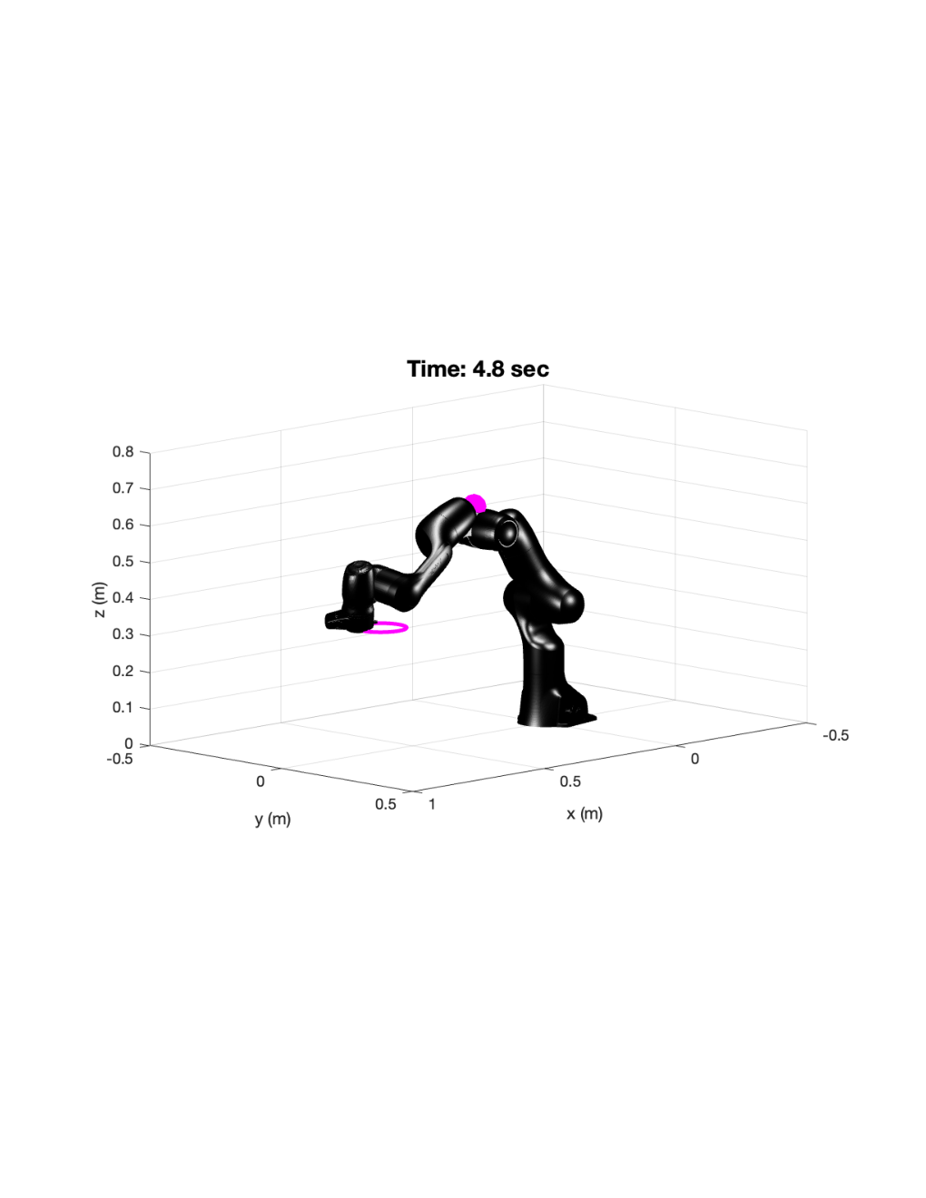
Thanks to the modularity of the implemented geometric method, the kinematics of any point on any body can be selected by specifying the robot body (’bodyID’) and the corresponding position on the body (’position’):

We compared the computational speed of Exp[licit] with the RVC MATLAB software[17], which uses the DH-convention. For RVC, version RTB10+MVTB4 (2017) was used.⁶⁶ 6 The software can be downloaded at https://petercorke.com/toolboxes/robotics-toolbox/ By using native MATLAB scripts, the computation time was compared for the Forward Kinematic Map, Hybrid Jacobian, Mass Matrix, centrifugal/Coriolis terms, and Gravity vector of an $n$-DOF open-chain planar robot. The robot consisted of $n$ identical uniform-mass bars with length $l=$ 1m and mass $m=$ 1kg. While Exp[licit] calculates the gravity and centrifugal/Coriolis terms with a closed-form algorithm, RVC use recursive Newton-Euler methods (RNE). Both, Exp[licit] and RVC uses .m-MATLAB scripts. For the mass matrix, gravity and the centrifugal/Coriolis effects, the RVC-Method can invoke MEX-files to improve the computation speed. MEX-files are native C or C++ files that are dynamically linked to the MATLAB application at runtime.

For the RVC software, the robot was constructed from the SerialLink-class which consists of $n$ Revolute-classes. For Exp[licit], the robot was constructed from the SnakeBot-class (fig. 4A). Robots with various DOF were constructed and tested. The test was performed with a MacBook air (M1 Chip, 16GB Memory), using MATLAB 2022a. The timeit() function was used to measure the computation time.

The results of our computational comparisons are shown in Figure 1. For almost all computations, Exp[licit] was faster than the RVC software. Only for more than 70 DOF, the gravity vector of the RVC MEX-file option was faster than Exp[licit]. For both software, the computation of the Forward Kinematic Map and the Hybrid Jacobian showed a linear trend. The RVC software was capable of computing the Forward Kinematic Map of a 15-DOF robot within 1ms, whereas Exp[licit] required less than 0.5ms for more than 100 DOF. For the Hybrid Jacobian, the RVC software required more than 1ms for a 15-DOF robot, while Exp[licit] could accomplish the same for 80 DOF. The computation of the Mass Matrix showed an exponential trend for both software. While Exp[licit] outperformed RCV for MATLAB scripts by a factor of 100, RVC had a much better performance using MEX-files. Nevertheless, it was still slower than Exp[licit]. A similar trend was seen for the gravity vector: RVC’s performance was improved by invoking MEX-files and showed better performance for more than 70 DOF. However, for the centrifugal/Coriolis terms, Exp[licit] drastically outperformed RCV.

These results highlight the computational advantages of a geometric approach, theoretically discussed in [28].

References

- [1] J. J. Craig, Introduction to robotics : mechanics & control / John J. Craig. Reading, Mass.: Addison-Wesley Pub. Co.,, 1986.
- [2] B. Siciliano, L. Sciavicco, L. Villani, and G. Oriolo, Robotics: Modelling, Planning and Control. Springer Publishing Company, Incorporated, 2010.
- [3] C. Nainer, M. Feder, and A. Giusti, “Automatic generation of kinematics and dynamics model descriptions for modular reconfigurable robot manipulators,” 2021 IEEE 17th International Conference on Automation Science and Engineering (CASE), pp. 45–52, 2021.
- [4] K. M. Lynch and F. C. Park, Modern robotics. Cambridge University Press, 2017.
- [5] C. Rocha, C. Tonetto, and A. Dias, “A comparison between the denavit–hartenberg and the screw-based methods used in kinematic modeling of robot manipulators,” Robotics and Computer-Integrated Manufacturing, vol. 27, no. 4, pp. 723–728, 2011.
- [6] S. Stramigioli, “From differentiable manifolds to interactive robot control,” Ph.D. dissertation, University of Delft, Netherlands, 1998.
- [7] J. Lachner, “A geometric approach to robotic manipulation in physical human-robot interaction,” Ph.D. dissertation, University of Twente, Netherlands, 2022.
- [8] R. Murray, Z. Li, S. Sastry, and S. Sastry, A Mathematical Introduction to Robotic Manipulation. Taylor & Francis, 1994.
- [9] J. M. Selig, Geometric fundamentals of robotics. New York: Springer, 2005.
- [10] S. Stramigioli and H. Bruyninckx, “Tutorial: Geometry and screw theory for robotics,” in 2001 IEEE International Conference on Robotics and Automation (ICRA), 2001.
- [11] A. Mueller, “Screw and lie group theory in multibody dynamics,” Multibody System Dynamics, vol. 42, pp. 219–248, 2018.
- [12] F. C. Park, B. Kim, C. Jang, and J. Hong, “Geometric Algorithms for Robot Dynamics: A Tutorial Review,” Applied Mechanics Reviews, vol. 70, no. 1, p. 010803, 02 2018. [Online]. Available: https://doi.org/10.1115/1.4039078
- [13] F. Park, “Computational aspects of the product-of-exponentials formula for robot kinematics,” IEEE transactions on automatic control., vol. 39, no. 3, pp. 643–647, 1994.
- [14] A. Mueller, “Recursive second-order inverse dynamics for serial manipulators,” in 2017 IEEE International Conference on Robotics and Automation (ICRA), 2017, pp. 2483–2489.
- [15] R. Tedrake and the Drake Development Team, “Drake: Model-based design and verification for robotics,” 2019. [Online]. Available: https://drake.mit.edu
- [16] E. Rohmer, S. P. N. Singh, and M. Freese, “Coppeliasim (formerly v-rep): a versatile and scalable robot simulation framework,” in Proc. of The International Conference on Intelligent Robots and Systems (IROS), 2013.
- [17] P. Corke and O. Khatib, Robotics, Vision and Control - Fundamental Algorithms in MATLAB, ser. Springer Tracts in Advanced Robotics. Springer, 2011, vol. 73.
- [18] E. Todorov, T. Erez, and Y. Tassa, “Mujoco: A physics engine for model-based control,” in 2012 IEEE/RSJ International Conference on Intelligent Robots and Systems, 2012, pp. 5026–5033.
- [19] M. L. Felis, “Rbdl: an efficient rigid-body dynamics library using recursive algorithms,” Autonomous Robots, pp. 1–17, 2016.
- [20] J. Denavit and R. S. Hartenberg, “A kinematic notation for lower-pair mechanisms based on matrices,” Trans. ASME E, Journal of Applied Mechanics, vol. 22, pp. 215–221, June 1955.
- [21] J. Angeles, Fundamentals of Robotic Mechanical Systems: Theory, Methods, and Algorithms (Mechanical Engineering Series). Berlin, Heidelberg: Springer-Verlag, 2006.
- [22] B. Siciliano and O. Khatib, Springer Handbook of Robotics. Berlin, Heidelberg: Springer-Verlag, 2007.
- [23] R. W. Brockett, Robotic manipulators and the product of exponentials formula. Berlin, Heidelberg: Springer Berlin Heidelberg, 1984.
- [24] S. Stramigioli, Modeling and IPC control of interactive mechanical systems—A coordinate-free approach. Springer, 2001.
- [25] F. Emika, “Robot and interface specifications,” https://frankaemika.github.io/docs/control_parameters.html, 2027.
- [26] J.-J. E. Slotine and W. Li, “On the adaptive control of robot manipulators,” The international journal of robotics research, vol. 6, no. 3, pp. 49–59, 1987.
- [27] N. Hogan, “Impedance control (an approach to manipulation) part i, ii, iii,” Trans the ASME, J. of Dynamic systems, Measurement and Control, vol. 107, pp. 1–24, 1985.
- [28] F. C. Park, “Computational aspects of the product-of-exponentials formula for robot kinematics,” IEEE Transactions on Automatic Control, vol. 39, no. 3, pp. 643–647, 1994.