跳到论文正文
W Papers独立论文阅读器 arXiv:2309.06563 论文正文 计算阅读时间 · 0%
引用这篇论文根据当前论文元数据生成,正式投稿前建议核对。


License: CC BY 4.0
arXiv:2309.06563v1 [math.ST] 12 Sep 2023

On Robust Recovery of Signals from Indirect Observations

Yannis Bekri Thanks: LJK, Université Grenoble Alpes, Campus de Saint-Martin-d’Hères, 38401 France    Anatoli JuditskyArkadi Nemirovski Thanks: Georgia Institute of Technology, Atlanta, Georgia 30332, USA
Abstract

Our focus is on robust recovery algorithms in statistical linear inverse problem. We consider two recovery routines—the much-studied linear estimate originating from Kuks and Olman [42] and polyhedral estimate introduced in [37]. It was shown in [38] that risk of these estimates can be tightly upper-bounded for a wide range of a priori information about the model through solving a convex optimization problem, leading to a computationally efficient implementation of nearly optimal estimates of these types. The subject of the present paper is design and analysis of linear and polyhedral estimates which are robust with respect to the uncertainty in the observation matrix. We evaluate performance of robust estimates under stochastic and deterministic matrix uncertainty and show how the estimation risk can be bounded by the optimal value of efficiently solvable convex optimization problem; “presumably good” estimates of both types are then obtained through optimization of the risk bounds with respect to estimate parameters.
 
2020 Mathematics Subject Classification: 62G05, 62G10, 90C90
Keywords: statistical linear inverse problems, robust estimation, observation matrix uncertainty

1 Introduction

In this paper we focus on the problem of recovering unknown signal xx given noisy observation ω∈𝐑m\omega\in{\mathbf{R}}^{m},

ω=A​x+ξ,\omega=Ax+\xi, (1)

of the linear image A​xAx of xx; here ξ∈𝐑m\xi\in{\mathbf{R}}^{m} is observation noise. Our objective is to estimate the linear image w=B​x∈𝐑νw=Bx\in{\mathbf{R}}^{\nu} of xx known to belong to given convex and compact subset 𝒳{\cal X} of 𝐑n{\mathbf{R}}^{n}. The estimation problem above is a classical linear inverse problem. When statistically analysed, popular approaches to solving  (1) (cf., e.g., [55, 31, 32, 50, 73, 40, 27, 65]) usually assume a special structure of the problem, when matrix AA and set 𝒳{\cal X} “fit each other,” e.g., there exists a sparse approximation of the set 𝒳{\cal X} in a given basis/pair of bases, in which matrix AA is “almost diagonal” (see, e.g. [16, 13] for detail). Under these assumptions, traditional results focus on estimation algorithms which are both numerically straightforward and statistically (asymptotically) optimal with closed form analytical description of estimates and corresponding risks. In this paper, AA and BB are “general” matrices of appropriate dimensions, and 𝒳{\cal X} is a rather general convex and compact set. Instead of deriving closed form expressions for estimates and risks (which under the circumstances seems to be impossible), we adopt an “operational” approach initiated in [15] and further developed in [34, 36, 37, 38], within which both the estimate and its risk are yielded by efficient computation, rather than by an explicit analytical description.

In particular, two classes of estimates were analyzed in [36, 37, 38] in the operational framework.

  • •

    Linear estimates. Since their introduction in [43, 44], linear estimates are a standard part of the theoretical statistical toolkit. There is an extensive literature dealing with the design and performance analysis of linear estimates (see, e.g., [63, 17, 20, 18, 30, 71, 74]). When applied in the estimation problem we consider here, linear estimate w^linH​(ω)\widehat{w}_{\mathrm{lin}}^{H}(\omega) is of the form w^H​(ω)=HT​ω\widehat{w}_{H}(\omega)=H^{T}\omega and is specified by a contrast matrix H∈𝐑m×νH\in{\mathbf{R}}^{m\times\nu}.

  • •

    Polyhedral estimates. The idea of a polyhedral estimate goes back to [60] where it was shown (see also [58, Chapter 2]) that such estimate is near-optimal when recovering smooth multivariate regression function known to belong to a given Sobolev ball from noisy observations taken along a regular grid. It has been recently reintroduced in [23] and [65] and extended to the setting to follow in [37]. In this setting, a polyhedral estimate ω↦w^polyH​(ω)\omega\mapsto\widehat{w}^{H}_{\mathrm{poly}}(\omega) is specified by a contrast matrix H∈𝐑m×MH\in{\mathbf{R}}^{m\times M} according to

    ω↦x^H​(ω)∈Argminx∈𝒳⁡‖HT​(ω−A​x)‖∞↦w^polyH​(ω):=B​x^​(ω).\omega\mapsto{\widehat{x}}^{H}(\omega)\in\mathop{\hbox{\rm Argmin}}_{x\in{\cal X}}\|H^{T}(\omega-Ax)\|_{\infty}\mapsto\widehat{w}^{H}_{\mathrm{poly}}(\omega):=B{\widehat{x}}(\omega).

Our interest in these estimates stems from the results of [35, 37, 38] where it is shown that in the Gaussian case (ξ∼𝒩⁡(0,σ2​Im)\xi\sim{\cal N}(0,\sigma^{2}I_{m})), linear and polyhedral estimates with properly designed efficiently computable contrast matrices are near-minimax optimal in terms of their risks over a rather general class of loss functions and signal sets---ellitopes and spectratopes. 11 1 Exact definitions of these sets are reproduced in the main body of the paper. For the time being, it suffices to point out two instructive examples: the bounded intersections of finitely many sets of the form {x:‖P​x‖p≤1}\{x:\|Px\|_{p}\leq 1\}, p≥2p\geq 2, is an ellitope (and a spectratope as well), and the unit ball of the spectral norm in the space of m×nm\times n matrices is a spectratope.

In this paper we consider an estimation problem which is a generalization of that mentioned above in which observation matrix A∈𝐑m×nA\in{\mathbf{R}}^{m\times n} is uncertain. Specifically, we assume that

ω=A⁡[η]​x+ξ\omega=A[\eta]x+\xi (2)

where ξ∈𝐑m\xi\in{\mathbf{R}}^{m} is zero mean random noise and

A⁡[η]=A+∑α=1qηα​Aα∈𝐑m×nA[\eta]=A+{\sum}_{\alpha=1}^{q}\eta_{\alpha}A_{\alpha}\in{\mathbf{R}}^{m\times n} (3)

where A,A1,…,AqA,A_{1},...,A_{q} are given matrices and η∈𝐑q\eta\in{\mathbf{R}}^{q} is uncertain perturbation (“uncertainty” for short). We consider separately two situations: the first one in which the perturbation η\eta is random (“random perturbation”), and the second one with η\eta selected, perhaps in an adversarial fashion, from a given uncertainty set 𝒰{\cal U} (”uncertain-but-bounded perturbation”). Observation model  (2) with random uncertainty is related to the linear regression problem with random errors in regressors [5, 8, 21, 22, 45, 68, 72] which is usually addressed through total least squares. It can also be seen as alternative modeling of the statistical inverse problem in which sensing matrix is recovered with stochastic error (see, e.g., [10, 11, 19, 25, 27, 51]). Estimation from observations  (2) under uncertain-but-bounded perturbation of observation matrix can be seen as an extension of the problem of solving systems of equations affected by uncertainty which has received significant attention in the literature (cf., e.g., [14, 26, 41, 56, 61, 62, 64] and references therein). It is also tightly related to the system identification problem under uncertain-but-bounded perturbation of the observation of the state of the system [6, 9, 12, 33, 46, 52, 53, 57, 69].

In what follows, our goal is to extend the estimation constructions from [38] to the case of uncertain sensing matrix. Our strategy consists in constructing a tight efficiently computable convex in HH upper bound on the risk of a candidate estimate, and then building a “presumably good” estimate by minimizing this bound in the estimate parameter HH. Throughout the paper, we assume that the signal set 𝒳{\cal X} is an ellitope, and the norm ∥⋅∥\|\cdot\| quantifying the recovery error is the maximum of a finite collection of Euclidean norms.

Our contributions

can be summarized as follows.

  • A.

    In Section 2.1 we analyse the ϵ\epsilon-risk (the maximum, over signals from 𝒳{\cal X}, of the radii of (1−ϵ)(1-\epsilon)-confidence ∥⋅∥\|\cdot\|-balls) and the design of presumably good, in terms of this risk, linear estimates in the case of random uncertainty.

  • B.

    In Section 3.1, we build presumably good linear estimates in the case of structured norm-bounded uncertainty (cf. [1, Chapter 7] and references therein), thus extending the corresponding results of [33].

Developments in A and B lead to novel computationally efficient techniques for designing presumably good linear estimates for both random and uncertain-but-bounded perturbations.

Analysis and design of polyhedral estimates under uncertainty in sensing matrix form the subject of Sections 2.2 (random perturbations) and 3.2 (uncertain-but-bounded perturbations). The situation here is as follows:

  • C.

    The random perturbation case of the Analysis problem

    Given contrast matrix HH, find a provably tight efficiently computable upper bound on ϵ\epsilon-risk of the associated estimate

    is the subject of Section 2.2, where it is solved “in the full range” of our assumptions (ellitopic 𝒳{\cal X}, sub-Gaussian zero mean η\eta and ξ\xi). In contrast, the random perturbation case of the Synthesis problem in which we want to minimize the above bound w.r.t. HH turns out to be more involving—the bound to be optimized happens to be nonconvex in HH. When there is no uncertainty in sensing matrix, this difficulty can be somehow circumvented [38, Section 5.1]; however, when uncertainty in sensing matrix is present, the strategy developed in [38, Section 5.1] happens to work only when 𝒳{\cal X} is an ellipsoid rather than a general-type ellitope. The corresponding developments are the subject of Sections 2.2.4, 2.2.5, and 2.2.6.

  • D.

    In our context, analysis and design of polyhedral estimates under uncertain-but-bounded perturbations in the sensing matrix appears to be the most difficult; our very limited results on this subject form the subject of Section 3.2,

Notation and assumptions.

We denote with ∥⋅∥\|\cdot\| the norm on 𝐑ν{\mathbf{R}}^{\nu} used to measure the estimation error. In what follows, ∥⋅∥\|\cdot\| is a maximum of Euclidean norms

‖u‖=maxℓ≤L⁡uT​Rℓ​u\|u\|=\max_{\ell\leq L}\sqrt{u^{T}R_{\ell}u} (4)

where Rℓ∈𝐒+νR_{\ell}\in{\mathbf{S}}^{\nu}_{+}, ℓ=1,…,L\ell=1,...,L, are given matrices with ∑ℓRℓ≻0{\sum}_{\ell}R_{\ell}\succ 0.

Throughout the paper, unless otherwise is explicitly stated, we assume that observation noise ξ\xi is zero-mean sub-Gaussian, ξ∼𝒮𝒢⁡(0,σ2​I)\xi\sim{\cal SG}(0,\sigma^{2}I), i.e., for all t∈𝐑mt\in{\mathbf{R}}^{m},

𝐄⁡{etT​ξ}≤exp⁡(σ22​‖t‖22).\displaystyle{\mathbf{E}}\left\{e^{t^{T}\xi}\right\}\leq\exp\left(\tfrac{\sigma^{2}}{2}{\|t\|_{2}^{2}}\right). (5)

2 Random perturbations

In this section we assume that uncertainty η\eta is sub-Gaussian, with parameters 0,I0,I, i.e.,

𝐄⁡{etT​η}≤exp⁡(12​‖t‖22)∀t∈𝐑q.\displaystyle{\mathbf{E}}\left\{e^{t^{T}\eta}\right\}\leq\exp\left(\tfrac{1}{2}{\|t\|_{2}^{2}}\right)\quad\forall t\in{\mathbf{R}}^{q}. (6)

In this situation, given ϵ∈(0,1)\epsilon\in(0,1), we quantify the quality of recovery w^​(⋅){\widehat{w}}(\cdot) of w=B​xw=Bx by its maximal over x∈𝒳x\in{\cal X} ϵ\epsilon-risk

Riskϵ[w^|𝒳]:=supx∈𝒳inf{ρ:Probξ,η{∥Bx−w^(A[η]x+ξ)∥>ρ}≤ϵ}\displaystyle{\hbox{\rm Risk}}_{\epsilon}[{\widehat{w}}|{\cal X}]:=\sup_{x\in{\cal X}}\inf\left\{\rho:\,\hbox{\rm Prob}_{\xi,\eta}\{\|Bx-\widehat{w}(A[\eta]x+\xi)\|>\rho\}\leq\epsilon\right\} (7)

(the radius of the smallest ∥⋅∥\|\cdot\|-ball centered at w^​(ω){\widehat{w}}(\omega) which covers xx, uniformly over x∈𝒳x\in{\cal X}).

2.1 Design of presumably good linear estimate

2.1.1 Preliminaries: ellitopes

Throughout this section, we assume that the signal set 𝒳{\cal X} is a basic ellitope. Recall that, by definition [35, 38], a basic ellitope in 𝐑n{\mathbf{R}}^{n} is a set of the form

𝒳={x∈𝐑n:∃t∈𝒯:zTTkz≤tk,k≤K},\displaystyle{\cal X}=\{x\in{\mathbf{R}}^{n}:\,\exists t\in{\cal T}:\,z^{T}T_{k}z\leq t_{k},\,k\leq K\}, (8)

where Tk∈𝐒+nT_{k}\in{\mathbf{S}}^{n}_{+}, Tk⪰0T_{k}\succeq 0, ∑kTk≻0{\sum}_{k}T_{k}\succ 0, and 𝒯⊂𝐑+K{\cal T}\subset{\mathbf{R}}^{K}_{+} is a convex compact set with a nonempty interior which is monotone: whenever 0≤t′≤t∈𝒯0\leq t^{\prime}\leq t\in{\cal T} one has t′∈𝒯t^{\prime}\in{\cal T}. We refer to KK as ellitopic dimension of 𝒳{\cal X}.

Clearly, every basic ellitope is a convex compact set with nonempty interior which is symmetric w.r.t. the origin. For instance,
A. Bounded intersection 𝒳{\cal X} of KK centered at the origin ellipsoids/elliptic cylinders {x∈𝐑n:xT​Tk​x≤1}\{x\in{\mathbf{R}}^{n}:x^{T}T_{k}x\leq 1\} [Tk⪰0T_{k}\succeq 0] is a basic ellitope:

𝒳={x∈𝐑n:∃t∈𝒯:=[0,1]K:xTTkx≤tk,k≤K}{\cal X}=\{x\in{\mathbf{R}}^{n}:\exists t\in{\cal T}:=[0,1]^{K}:x^{T}T_{k}x\leq t_{k},\,k\leq K\}

In particular, the unit box {x∈𝐑n:‖x‖∞≤1}\{x\in{\mathbf{R}}^{n}:\|x\|_{\infty}\leq 1\} is a basic ellitope.
B. A ∥⋅∥p\|\cdot\|_{p}-ball in 𝐑n{\mathbf{R}}^{n} with p∈[2,∞]p\in[2,\infty] is a basic ellitope:

{x∈𝐑n:∥x∥p≤1}={x:∃t∈𝒯={t∈𝐑+n,∥t∥p/2≤1}:xk2⏟xT​Tk​x≤tk,k≤K}.\{x\in{\mathbf{R}}^{n}:\|x\|_{p}\leq 1\}=\big\{x:\exists t\in{\cal T}=\{t\in{\mathbf{R}}^{n}_{+},\|t\|_{p/2}\leq 1\}:\underbrace{x_{k}^{2}}_{x^{T}T_{k}x}\leq t_{k},\,k\leq K\big\}.

In the present context, our interest for ellitopes is motivated by their special relationship with the optimization problem

Opt∗​(C)=maxx∈𝒳⁡xT​C​x,C∈𝐒n\hbox{\rm Opt}_{*}(C)=\max\limits_{x\in{\cal X}}x^{T}Cx,\,\,C\in{\mathbf{S}}^{n} (9)

of maximizing a homogeneous quadratic form over 𝒳{\cal X}. As it is shown in [38], when 𝒳{\cal X} is an ellitope,  (9) admits “reasonably tight” efficiently computable upper bound. Specifically,

Theorem 2.1

[38, Proposition 4.6] Given ellitope  (8) and matrix CC, consider the quadratic maximization problem (9) along with its relaxation22 2 Here and below, we use notation ϕ𝒮​(⋅)\phi_{\cal S}(\cdot) for the support function of a convex set 𝒮⊂𝐑n{\cal S}\subset{\mathbf{R}}^{n}: for y∈𝐑ny\in{\mathbf{R}}^{n}, ϕ𝒮​(y)=supu∈𝒮yT​s.\phi_{\cal S}(y)=\sup_{u\in{\cal S}}y^{T}s.

Opt(C)=minλ{ϕ𝒯(λ):λ≥0,∑kλkTk−C⪰0}\hbox{\rm Opt}(C)=\min_{\lambda}\left\{\phi_{{\cal T}}(\lambda):\lambda\geq 0,{{\sum}}_{k}\lambda_{k}T_{k}-C\succeq 0\right\} (10)

The problem is computationally tractable and solvable, and Opt​(C)\hbox{\rm Opt}(C) is an efficiently computable upper bound on Opt∗​(C)\hbox{\rm Opt}_{*}(C). This upper bound is tight:

Opt∗​(C)≤Opt​(C)≤3​ln⁡(3​K)​Opt∗​(C).\hbox{\rm Opt}_{*}(C)\leq\hbox{\rm Opt}(C)\leq 3\ln(\sqrt{3}K)\hbox{\rm Opt}_{*}(C).

2.1.2 Tight upper bounding the risk of linear estimate

Consider a linear estimate

w^H(ω)=HTω[H∈𝐑m×ν]\widehat{w}^{H}(\omega)=H^{T}\omega\quad[H\in{\mathbf{R}}^{m\times\nu}]
Proposition 2.1

In the setting of this section, synthesis of a presumably good linear estimate reduces to solving the convex optimization problem

minH∈𝐑m×ν⁡ℜ⁡[H]\displaystyle\min\limits_{H\in{\mathbf{R}}^{m\times\nu}}{{\mathfrak{R}}}[H] (11)

where

ℜ⁡[H]=minλℓ,μℓ,κℓ,ϰℓ,ρ,ϱ{[1+2​ln⁡(2​L/ϵ)][σmaxℓ≤L∥HRℓ1/2∥Fro+ρ]+ϱ:μℓ≥0,ϰℓ≥0,λℓ+ϕ𝒯​(μℓ)≤ρ,κℓ+ϕ𝒯​(ϰℓ)≤ϱ,ℓ≤L[λℓ​Iν​q12​[Rℓ1/2​HT​A1;…;Rℓ1/2​HT​Aq]12​[A1T​H​Rℓ1/2,…,AqT​H​Rℓ1/2]∑kμkℓ​Tk]⪰0,ℓ≤L[κℓ​Iν12​Rℓ1/2​[B−HT​A]12​[B−HT​A]T​Rℓ1/2∑kϰkℓ​Tk]⪰0,ℓ≤L}\begin{array}[]{rcl}{{\mathfrak{R}}}[H]&=&\min_{\lambda_{\ell},\mu^{\ell},\kappa^{\ell},\atop\varkappa^{\ell},\rho,\varrho}\bigg\{\left[1+\sqrt{2\ln(2L/\epsilon)}\right]\left[\sigma\max\limits_{\ell\leq L}\|HR_{\ell}^{1/2}\|_{\mathrm{Fro}}+\rho\right]+\varrho:\\ &&\left.\begin{array}[]{l}\mu^{\ell}\geq 0,\varkappa^{\ell}\geq 0,\,\lambda_{\ell}+\phi_{\cal T}(\mu_{\ell})\leq\rho,\kappa_{\ell}+\phi_{\cal T}(\varkappa^{\ell})\leq\varrho,\,\ell\leq L\\ \hbox{\scriptsize$\left[\begin{array}[]{c|c}\lambda_{\ell}I_{\nu q}&{1\over 2}\left[R_{\ell}^{1/2}H^{T}A_{1};...;R_{\ell}^{1/2}H^{T}A_{q}\right]\cr\hline\cr{1\over 2}\left[A_{1}^{T}HR_{\ell}^{1/2},...,A_{q}^{T}HR_{\ell}^{1/2}\right]&{\sum}_{k}\mu^{\ell}_{k}T_{k}\cr\end{array}\right]$}\succeq 0,\,\ell\leq L\\ \hbox{\scriptsize$\left[\begin{array}[]{c|c}\kappa^{\ell}I_{\nu}&{1\over 2}R_{\ell}^{1/2}[B-H^{T}A]\cr\hline\cr{1\over 2}[B-H^{T}A]^{T}R_{\ell}^{1/2}&{\sum}_{k}\varkappa^{\ell}_{k}T_{k}\cr\end{array}\right]$}\succeq 0,\,\ell\leq L\\ \end{array}\right\}\\ \end{array} (12)

For a candidate contrast matrix HH, the ϵ\epsilon-risk of the linear estimate w^linH​(ω)=HT​ω\widehat{w}^{H}_{\mathrm{lin}}(\omega)=H^{T}\omega is upper-bounded by ℜ⁡[H]{{\mathfrak{R}}}[H].

2.1.3 A modification

Let us assume that a KK-repeated version of observation (2) is available, i.e., we observe

ωK={ωk=A⁡[ηk]​x+ξk,k=1,…,K}\omega^{K}=\{\omega_{k}=A[\eta_{k}]x+\xi_{k},\,k=1,...,K\} (13)

with independent across kk pairs (ξk,ηk)(\xi_{k},\eta_{k}). In this situation, we can relax the assumption of sub-Gaussianity of ξ\xi and η\eta to the second moment boundedness condition

𝐄⁡{ξ​ξT}⪯σ2​Im,𝐄⁡{η​ηT}⪯Iq.{\mathbf{E}}\{\xi\xi^{T}\}\preceq\sigma^{2}I_{m},\quad{\mathbf{E}}\left\{\eta\eta^{T}\right\}\preceq I_{q}. (14)

Let us consider the following construction. For each ℓ≤L\ell\leq L, given H∈𝐑m×νH\in{\mathbf{R}}^{m\times\nu} we denote

ℜ~ℓ​[H]=minλ,μ,κ,ϰ{σ∥HRℓ1/2∥Fro+λ+ϕ𝒯(μ)+κ+ϕ𝒯(ϰ):μ≥0,ϰ≥0,[κ​Iν12​Rℓ1/2​[B−HT​A]12​[B−HT​A]T​Rℓ1/2∑kϰk​Tk]⪰0[λ​Iν​q12​[Rℓ1/2​HT​A1;…;Rℓ1/2​HT​Aq]12​[A1T​H​Rℓ1/2,…,AqT​H​Rℓ1/2]∑kμk​Tk]⪰0}\begin{array}[]{rcl}\widetilde{{\mathfrak{R}}}_{\ell}[H]&=&\min_{\lambda,\mu,\kappa,\varkappa}\bigg\{\sigma\|HR_{\ell}^{1/2}\|_{\mathrm{Fro}}+\lambda+\phi_{\cal T}(\mu)+\kappa+\phi_{\cal T}(\varkappa):\\ &&\left.\begin{array}[]{l}\mu\geq 0,\varkappa\geq 0,\left[\begin{array}[]{c|c}\kappa I_{\nu}&{1\over 2}R_{\ell}^{1/2}[B-H^{T}A]\cr\hline\cr{1\over 2}[B-H^{T}A]^{T}R_{\ell}^{1/2}&{\sum}_{k}\varkappa_{k}T_{k}\cr\end{array}\right]\succeq 0\\ \left[\begin{array}[]{c|c}\lambda I_{\nu q}&{1\over 2}\left[R_{\ell}^{1/2}H^{T}A_{1};...;R_{\ell}^{1/2}H^{T}A_{q}\right]\cr\hline\cr{1\over 2}\left[A_{1}^{T}HR_{\ell}^{1/2},...,A_{q}^{T}HR_{\ell}^{1/2}\right]&{\sum}_{k}\mu_{k}T_{k}\cr\end{array}\right]\succeq 0\end{array}\right\}\end{array} (15)

and consider the convex optimization problem

H~ℓ∈ArgminH⁡ℜ~ℓ​[H].\widetilde{H}_{\ell}\in\mathop{\hbox{\rm Argmin}}_{H}\widetilde{{\mathfrak{R}}}_{\ell}[H]. (16)

We define the “reliable estimate” w^(r)​(ωK){\widehat{w}}^{(r)}(\omega^{K}) of w=B​xw=Bx as follows.

  1. 1.

    Given Hℓ∈𝐑m×νH_{\ell}\in{\mathbf{R}}^{m\times\nu} and observations ωk\omega_{k} we compute linear estimates wℓ​(ωk)=Hℓ​ωkw_{\ell}(\omega_{k})=H_{\ell}\omega_{k}, ℓ=1,…,L,k=1,…,K\ell=1,...,L,\,k=1,...,K;

  2. 2.

    We define vectors zℓ∈𝐑νz_{\ell}\in{\mathbf{R}}^{\nu} as geometric medians of wℓ​(ωk)w_{\ell}(\omega_{k}):

    zℓ(ωK)∈Argminz∑k=1K∥Rℓ1/2(wℓ(ωk)−z)∥2,ℓ=1,…,L.z_{\ell}(\omega^{K})\in\mathop{\hbox{\rm Argmin}}_{z}\sum_{k=1}^{K}\|R_{\ell}^{1/2}(w_{\ell}(\omega_{k})-z)\|_{2},\;\ell=1,...,L.
  3. 3.

    Finally, we select as w^(r)​(ωK){\widehat{w}}^{(r)}(\omega^{K}) any point of the set

    𝒲⁡(ωK)=⋂ℓ=1L{w∈𝐑ν:‖Rℓ1/2​(zℓ​(ωK)−w)‖2≤4​ℜ~ℓ​[Hℓ]}.{\cal W}(\omega^{K})=\bigcap_{\ell=1}^{L}\left\{w\in{\mathbf{R}}^{\nu}:\,\|R_{\ell}^{1/2}(z_{\ell}(\omega^{K})-w)\|_{2}\leq 4\widetilde{{{\mathfrak{R}}}}_{\ell}[H_{\ell}]\right\}.

    or set w^(r)​(ωK){\widehat{w}}^{(r)}(\omega^{K}) a once for ever fixed point, e.g., w^(r)​(ωK)=0{\widehat{w}}^{(r)}(\omega^{K})=0 if 𝒲⁡(ωK)=∅{\cal W}(\omega^{K})=\emptyset.

We have the following analog of Proposition 2.1.

Proposition 2.2

In the situation of this section, it holds

supx∈𝒳𝐄ηk,ξk​{‖Rℓ1/2​(wℓ​(ωk)−B​x)‖22}≤ℜ~ℓ2​[Hℓ],ℓ≤L,\displaystyle\sup_{x\in{\cal X}}{\mathbf{E}}_{\eta_{k},\xi_{k}}\left\{\|R_{\ell}^{1/2}(w_{\ell}(\omega_{k})-Bx)\|_{2}^{2}\right\}\leq\widetilde{{\mathfrak{R}}}^{2}_{\ell}[H_{\ell}],\;\ell\leq L, (17)

and

Prob{∥Rℓ1/2(zℓ(ωK)−Bx)∥2≥4ℜ~ℓ[Hℓ]}≤e−0.1070​K,ℓ≤L.\displaystyle\hbox{\rm Prob}\left\{\|R_{\ell}^{1/2}(z_{\ell}(\omega^{K})-Bx)\|_{2}\geq 4\widetilde{{{\mathfrak{R}}}}_{\ell}[H_{\ell}]\right\}\leq e^{-0.1070K},\;\ell\leq L. (18)

As a consequence, whenever K≥ln⁡[L/ϵ]/0.1070K\geq\ln[L/\epsilon]/0.1070, the ϵ\epsilon-risk of the aggregated estimate w^(r)​(ωK){\widehat{w}}^{(r)}(\omega^{K}) satisfies

Riskϵ​[w^(r)​(ωK)|𝒳]≤ℜ¯,ℜ¯=8​maxℓ≤L​ℜ~ℓ​[Hℓ].{\hbox{\rm Risk}}_{\epsilon}[{\widehat{w}}^{(r)}(\omega^{K})|{\cal X}]\leq\overline{{{\mathfrak{R}}}},\;\;\overline{{{\mathfrak{R}}}}=8\max_{\ell\leq L}\widetilde{{{\mathfrak{R}}}}_{\ell}[H_{\ell}].
Remark.

Proposition 2.2 is motivated by the desire to capture situations in which sub-Gaussian assumption on η\eta and ξ\xi does not hold or is too restrictive. Consider, e.g., the case where the uncertainty in the sensing matrix reduces to zeroing out some randomly selected columns in the nominal matrix A¯\overline{A} (think of taking picture through the window with frost patterns). Denoting by γ\gamma the probability to zero out a particular column and assuming that columns are zeroed out independently, model (2) in this situation reads

ω=A⁡[η]​x+ξ,A⁡[η]=(1−γ)​A¯+∑α=1nηα​Aα\omega=A[\eta]x+\xi,\,A[\eta]=(1-\gamma)\overline{A}+{\sum}_{\alpha=1}^{n}\eta_{\alpha}A_{\alpha}

where η1,…,ηn\eta_{1},...,\eta_{n} are i.i.d. zero mean random variables taking values (γ−1)​ρ(\gamma-1)\rho and γ​ρ\gamma\rho with probabilities γ\gamma and 1−γ1-\gamma, and AαA_{\alpha}, 1≤α≤n1\leq\alpha\leq n, is an m×nm\times n matrix with all but the α\alpha-th column being zero and Colα​[Aα]=ρ−1​Colα​[A¯]{\hbox{\rm Col}}_{\alpha}[A_{\alpha}]=\rho^{-1}{\hbox{\rm Col}}_{\alpha}[\overline{A}]. Scaling factor ρ\rho is selected to yield the unit sub-Gaussianity parameter of η\eta or 𝐄⁡{ηα2}=1{\mathbf{E}}\{\eta_{\alpha}^{2}\}=1 depending on whether Proposition 2.1 or Proposition 2.2 is used. For small γ\gamma, the scaling factor ρ\rho is essentially smaller in the first case, resulting in larger “disturbance matrices” AαA_{\alpha} and therefore—in stricter constraints in the optimization problem  (11),  (12) responsible for the design of the linear estimate.

2.1.4 Numerical illustration
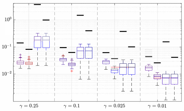
Refer to caption
Figure 1: Distributions of ℓ2\ell_{2}-recovery errors and upper bounds of the robust and “nominal” estimates for different values of γ\gamma parameter.

In Figure 1 we present results of a toy experiment in which

  • •

    n=32,m=32n=32,m=32, and ν=16\nu=16, A¯​x∈𝐑m\overline{A}x\in{\mathbf{R}}^{m} is the discrete time convolution of x∈𝐑nx\in{\mathbf{R}}^{n} with a simple kernel ϰ\varkappa of length 99 restricted onto the “time horizon” {1,…,n}\{1,...,n\}, and B​xBx cuts off xx the first ν\nu entries. We consider Gaussian perturbation η∼𝒩⁡(0,γ2​Iq)\eta\sim{\cal N}(0,\gamma^{2}I_{q}), q=9q=9, and A⁡[η]​x=[A+∑α=1qηα​Aα]​xA[\eta]x=[A+\sum_{\alpha=1}^{q}\eta_{\alpha}A_{\alpha}]x which is the convolution of xx with the kernel ϰη\varkappa_{\eta} restricted onto the time horizon {1,…,n}\{1,...,n\}, γ\gamma being the control parameter.

  • •

    L=1L=1 and ∥⋅∥=∥⋅∥2\|\cdot\|=\|\cdot\|_{2},

  • •

    𝒳{\cal X} is the ellipsoid {x:∑ii2​[D​x]i2≤1}\{x:\sum_{i}i^{2}[Dx]_{i}^{2}\leq 1\}, where DD is the matrix of inverse Discrete Cosine Transform of size n×nn\times n.

  • •

    ξ∼𝒩⁡(0,σ2​Im)\xi\sim{\cal N}(0,\sigma^{2}I_{m}), σ=10−4\sigma=10^{-4}.

In each cell of the plot we represent error distributions and upper risk bounds (horizontal bar) of four estimates (from left to right) for different uncertainty levels γ\gamma: (1) robust estimate by Proposition 2.1 and upper bound ℜ{{\mathfrak{R}}} on its 0.050.05-risk, (2) single-observation estimate w1​(ω1)=H1​ω1w_{1}(\omega_{1})=H_{1}\omega_{1} yielded by the minimizer H1H_{1} of ℜ~1​[H]\widetilde{{{\mathfrak{R}}}}_{1}[H] over HH, see (15), and upper bound ℜ~1​[H1]\widetilde{{{\mathfrak{R}}}}_{1}[H_{1}] on its expected error risk,33 3 We define expected error risk of a KK-observation estimate x^​(ωK)\widehat{x}(\omega^{K}) of B​xBx as supx∈𝒳𝐄ωK∼PxK​{‖x^​(ωK)−B​x‖}\sup_{x\in{\cal X}}{\mathbf{E}}_{\omega^{K}\sim P^{K}_{x}}\{\|\widehat{x}(\omega^{K})-Bx\|\}, where PxKP^{K}_{x} is the distribution of ωK\omega^{K} stemming from xx. (3) “nominal” estimate—estimate by Proposition 2.1 as applied to the “no uncertainty” case where all AαA_{\alpha} in (3) are set to 0 and upper bound ℜ{{\mathfrak{R}}} from  (12) on its 0.050.05-risk computed using actual uncertainty level, (4) “nominal” estimate w~1​(ω1)=H~1​ω1\widetilde{w}_{1}(\omega_{1})=\widetilde{H}_{1}\omega_{1} yielded by the minimizer H~1\widetilde{H}_{1} of ℜ~1​[H]\widetilde{{{\mathfrak{R}}}}_{1}[H] over HH in the “no uncertainty” case and upper bound ℜ~1​[H~1]\widetilde{{{\mathfrak{R}}}}_{1}[\widetilde{H}_{1}] on its “actual”—with uncertainty present—expected error risk.

2.2 Design of presumably good polyhedral estimate

2.2.1 Preliminaries on polyhedral estimates

Consider a slightly more general than (2), (3) observation scheme

ω=A​x+ζ\omega=Ax+\zeta (19)

where A∈𝐑m×nA\in{\mathbf{R}}^{m\times n} is given, unknown signal xx is known to belong to a given signal set 𝒳{\cal X} given by (8), and ζ\zeta is observation noise with probability distribution PxP_{x} which can depend on xx. For example, when observation ω\omega is given by (2), (3), we have

ζ=∑α=1qηα​Aα​x+ξ\zeta={\sum}_{\alpha=1}^{q}\eta_{\alpha}A_{\alpha}x+\xi (20)

with zero mean sub-Gaussian η\eta and ξ\xi.

When building polyhedral estimate in the situation in question, one, given tolerance ϵ∈(0,1)\epsilon\in(0,1) and a positive integer MM, specifies a computationally tractable convex set ℋ{\cal H}, the larger the better, of vectors h∈𝐑mh\in{\mathbf{R}}^{m} such that

Probζ∼Px{|hTζ|>1}≤ϵ/M∀x∈𝒳.\hbox{\rm Prob}_{\zeta\sim P_{x}}\{|h^{T}\zeta|>1\}\leq\epsilon/M\quad\forall x\in{\cal X}. (21)

A polyhedral estimate w^H​(⋅)\widehat{w}^{H}(\cdot) is specified by contrast matrix H∈𝐑M×nH\in{\mathbf{R}}^{M\times n} restricted to have all columns in ℋ{\cal H} according to

ω↦x^H​(ω)∈Argminu∈𝒳⁡{‖HT​[A​u−ω]‖∞},w^polyH​(ω)=B​x^H​(ω).\omega\mapsto{\widehat{x}}^{H}(\omega)\in\mathop{\hbox{\rm Argmin}}_{u\in{\cal X}}\left\{\|H^{T}[Au-\omega]\|_{\infty}\right\},\;\widehat{w}^{H}_{\mathrm{poly}}(\omega)=B{\widehat{x}}^{H}(\omega). (22)

It is easily seen (cf. [38, Proposition 5.1.1]) that the ϵ\epsilon-risk  (7) of the above estimate is upper-bounded by the quantity

𝔭[H]=supy{∥By∥:y∈2𝒳,∥HTAy∥∞≤2}.{\mathfrak{p}}[H]=\sup_{y}\left\{\|By\|:y\in 2{\cal X},\|H^{T}Ay\|_{\infty}\leq 2\right\}.\ (23)

Indeed, let h1,…,hMh_{1},...,h_{M} be the columns of HH. For x∈𝒳x\in{\cal X} fixed, the inclusions hj∈ℋh_{j}\in{\cal H} imply that the PxP_{x}-probability of the event Zx={ζ:|ζT​hj|≤1​∀j≤M}Z_{x}=\{\zeta:|\zeta^{T}h_{j}|\leq 1\,\forall j\leq M\} is at least 1−ϵ1-\epsilon. When this event takes place, we have ‖HT​[ω−A​x]‖∞≤1\|H^{T}[\omega-Ax]\|_{\infty}\leq 1, which combines with x∈𝒳x\in{\cal X} to imply that ‖HT​[ω−A​x^H​(ω)]‖∞≤1\|H^{T}[\omega-A{\widehat{x}}^{H}(\omega)]\|_{\infty}\leq 1, so that ‖HT​A​[x−x^H​(ω)]‖∞≤2\|H^{T}A[x-{\widehat{x}}^{H}(\omega)]\|_{\infty}\leq 2, and besides this, x−x^H​(ω)∈2​𝒳x-{\widehat{x}}^{H}(\omega)\in 2{\cal X}, whence ‖B​x−w^polyH​(ω)‖≤𝔭⁡[H]\|Bx-\widehat{w}^{H}_{\mathrm{poly}}(\omega)\|\leq{\mathfrak{p}}[H] by definition of 𝔭⁡[H]{\mathfrak{p}}[H]. The bottom line is that whenever x∈𝒳x\in{\cal X} and ζ=ω−A​x∈Zx\zeta=\omega-Ax\in Z_{x}, which happens with PxP_{x}-probability at least 1−ϵ1-\epsilon, we have ‖B​x−w^polyH​(ω)‖≤𝔭⁡[H]\|Bx-\widehat{w}^{H}_{\mathrm{poly}}(\omega)\|\leq{\mathfrak{p}}[H], whence the ϵ\epsilon-risk of the estimate w^polyH\widehat{w}^{H}_{\mathrm{poly}} indeed is upper-bounded by 𝔭⁡[H]{\mathfrak{p}}[H].

To get a presumably good polyhedral estimate, one minimizes 𝔭⁡[H]{\mathfrak{p}}[H] over M×νM\times\nu matrices HH with columns from ℋ{\cal H}. Precise minimization is problematic, because 𝔭⁡[⋅]{\mathfrak{p}}[\cdot], while being convex, is usually difficult to compute. Thus, the design routine proposed in [37] goes via minimizing an efficiently computable upper bound on 𝔭⁡[H]{\mathfrak{p}}[H]. It is shown in [38, Section 5.1.5] that when 𝒳{\cal X} is ellitope (8) and ‖u‖=‖R​u‖2\|u\|=\|Ru\|_{2}, a reasonably tight upper bound on 𝔭⁡[H]{\mathfrak{p}}[H] is given by the efficiently computable function

𝔭+​[H]=2​minλ,μ,υ​{λ+ϕ𝒯​(μ)+∑iυi:μ≥0,υ≥0[λ​Iν12​R​B12​BT​RTAT​H​Diag​{υ}​HT​A+∑kμk​Tk]⪰0}.{\mathfrak{p}}_{+}[H]=2\min\limits_{\lambda,\mu,\upsilon}\left\{\lambda+\phi_{\cal T}(\mu)+{\sum}_{i}\upsilon_{i}:\begin{array}[]{l}\mu\geq 0,\upsilon\geq 0\\ \hbox{\scriptsize$\left[\begin{array}[]{c|c}\lambda I_{\nu}&{1\over 2}RB\cr\hline\cr{1\over 2}B^{T}R^{T}&A^{T}H\hbox{\rm Diag}\{\upsilon\}H^{T}A+{\sum}_{k}\mu_{k}T_{k}\cr\end{array}\right]\succeq 0$}\end{array}\right\}.

Synthesis of a presumably good polyhedral estimate reduces to minimizing the latter function in HH under the restriction Colj​[H]∈ℋ{\hbox{\rm Col}}_{j}[H]\in{\cal H}. Note that the latter problem still is nontrivial because 𝔭+{\mathfrak{p}}_{+} is nonconvex in HH.

Our objective here is to implement the outlined strategy in the case of observation ω\omega is given by  (2),  (3).

2.2.2 Specifying ℋ{\cal H}

Our first goal is to specify, given tolerance δ∈(0,1)\delta\in(0,1), a set ℋδ⊂𝐑m{\cal H}_{\delta}\subset{\mathbf{R}}^{m}, the larger the better, such that

h∈ℋδ,x∈𝒳⇒Probζ∼Px{|hTζ|>1}≤δ.h\in{\cal H}_{\delta},x\in{\cal X}\Rightarrow\hbox{\rm Prob}_{\zeta\sim P_{x}}\{|h^{T}\zeta|>1\}\leq\delta. (24)

Note that a “tight” sufficient condition for the validity of (24) is

Probξ{|hTξ|>1/2}\displaystyle\hbox{\rm Prob}_{\xi}\{|h^{T}\xi|>1/2\} ≤δ/2,\displaystyle\leq\delta/2, (25a)
Probη{|∑α=1q[hTAαx]ηα|>1/2}\displaystyle\hbox{\rm Prob}_{\eta}\left\{\left|{\sum}_{\alpha=1}^{q}[h^{T}A_{\alpha}x]\eta_{\alpha}\right|>1/2\right\} ≤δ/2,∀x∈𝒳.\displaystyle\leq\delta/2,\,\forall x\in{\cal X}. (25b)

Note that under the sub-Gaussian assumption  (5), hT​ξh^{T}\xi is itself sub-Gaussian, hT​ξ∼𝒮𝒢⁡(0,σ2​‖h‖22)h^{T}\xi\sim{\cal SG}(0,\sigma^{2}\|h\|_{2}^{2}); thus, a tight sufficient condition for  (25a) is

‖h‖2≤[σ​χ​(δ)]−1,χ⁡(δ)=2​2​ln⁡(2/δ).\|h\|_{2}\leq[\sigma\chi(\delta)]^{-1},\,\,\chi(\delta)=2\sqrt{2\ln(2/\delta)}. (26)

Furthermore, by  (6), r.v. ∑α=1q[hT​Aα​x]​ηα=hT​[A1​x,…,Aq​x]​η{\sum}_{\alpha=1}^{q}[h^{T}A_{\alpha}x]\eta_{\alpha}=h^{T}[A_{1}x,...,A_{q}x]\eta is sub-Gaussian with parameters 00 and ‖[hT​A1​x;…;hT​Aq​x]‖22\|[h^{T}A_{1}x;...;h^{T}A_{q}x]\|_{2}^{2}, implying the validity of  (25b) for a given xx whenever

‖[hT​A1​x;…;hT​Aq​x]‖2≤χ−1​(δ).\|[h^{T}A_{1}x;...;h^{T}A_{q}x]\|_{2}\leq\chi^{-1}(\delta).

We want this relation to hold true for every x∈𝒳x\in{\cal X}, that is, we want the operator norm ∥⋅∥𝒳,2\|\cdot\|_{{\cal X},2} of the mapping

x↦𝒜⁡[h]​x,𝒜⁡[h]=[hT​A1;hT​A2;…;hT​Aq]x\mapsto{\cal A}[h]x,\;{\cal A}[h]=[h^{T}A_{1};h^{T}A_{2};...;h^{T}A_{q}] (27)

induced by the norm ∥⋅∥𝒳\|\cdot\|_{\cal X} on the argument and the norm ∥⋅∥2\|\cdot\|_{2} on the image space to be upper-bounded by χ⁡(δ)\chi(\delta):

‖𝒜⁡[h]‖χ,2≤χ−1​(δ).\displaystyle\|{\cal A}[h]\|_{\chi,2}\leq\chi^{-1}(\delta). (28)

Invoking [33, Theorem 3.1] (cf. also the derivation in the proof of Proposition 2.1 in Section A.2), a tight sufficient condition for the latter relation is

Opt[h]:=minλ,μ{λ+ϕ𝒯(μ):μ≥0,[λ​Iq12​𝒜​[h]12​𝒜T​[h]∑kμk​Tk]≻0}≤χ−1(δ),\hbox{\rm Opt}[h]:=\min_{\lambda,\mu}\left\{\lambda+\phi_{\cal T}(\mu):\,\mu\geq 0,\,\left[\begin{array}[]{c|c}\lambda I_{q}&{\tfrac{1}{2}}{\cal A}[h]\cr\hline\cr{\tfrac{1}{2}}{\cal A}^{T}[h]&{\sum}_{k}\mu_{k}T_{k}\cr\end{array}\right]\succ 0\right\}\leq\chi^{-1}(\delta), (29)

tightness meaning that Opt​[h]\hbox{\rm Opt}[h] is within factor O⁡(1)​ln⁡(K+1)O(1)\sqrt{\ln(K+1)} of ‖𝒜⁡[h]‖𝒳,2\|{\cal A}[h]\|_{{\cal X},2}.

The bottom line is that with ℋδ{\cal H}_{\delta} specified by constraints (26) and  (28) (or by the latter replaced with its tight relaxation  (29)) we do ensure (24).

2.2.3 Bounding the risk of the polyhedral estimate w^H{\widehat{w}}^{H}

Proposition 2.3

In the situation of this section, let ϵ∈(0,1)\epsilon\in(0,1), and let H=[H1,…,HL]H=[H_{1},...,H_{L}] be m×M​Lm\times ML matrix with LL blocks Hℓ∈𝐑m×MH_{\ell}\in{\mathbf{R}}^{m\times M} such that Colj​[H]∈ℋδ{\hbox{\rm Col}}_{j}[H]\in{\cal H}_{\delta} for all j≤M​Lj\leq ML and δ=ϵ/M​L\delta=\epsilon/ML. Consider optimization problem

𝔭+​[H]\displaystyle{\mathfrak{p}}_{+}[H] =2minλℓ,μℓ,υℓ,ρ{ρ:μℓ≥0,υℓ≥0,λℓ+ϕ𝒯(μℓ)+∑j=1Mυjℓ≤ρ,ℓ≤L\displaystyle=2\min_{\lambda_{\ell},\mu^{\ell},\upsilon^{\ell},\rho}\left\{\rho:\,\mu^{\ell}\geq 0,\upsilon^{\ell}\geq 0,\,\lambda_{\ell}+\phi_{\cal T}(\mu^{\ell})+{\sum}_{j=1}^{M}\upsilon^{\ell}_{j}\leq\rho,\,\ell\leq L\right.
[λℓ​Iν12​Rℓ1/2​B12​BT​Rℓ1/2AT​Hℓ​Diag​{υℓ}​HℓT​A+∑kμkℓ​Tk]⪰0,ℓ≤L}.\displaystyle\qquad\qquad\qquad\left.\left[\begin{array}[]{c|c}\lambda_{\ell}I_{\nu}&{1\over 2}R_{\ell}^{1/2}B\cr\hline\cr{1\over 2}B^{T}R_{\ell}^{1/2}&A^{T}H_{\ell}\hbox{\rm Diag}\{\upsilon^{\ell}\}H_{\ell}^{T}A+{\sum}_{k}\mu^{\ell}_{k}T_{k}\cr\end{array}\right]\succeq 0,\,\ell\leq L\right\}.

Then

Riskϵ​[w^H|𝒳]≤𝔭+​[H].{\hbox{\rm Risk}}_{\epsilon}[\widehat{w}^{H}|{\cal X}]\leq{\mathfrak{p}}_{+}[H].

2.2.4 Optimizing 𝔭+​[H]{\mathfrak{p}}_{+}[H]—the strategy

Proposition 2.3 resolves the analysis problem—it allows to efficiently upper-bound the ϵ\epsilon-risk of a given polyhedral estimate w^polyH{\widehat{w}}^{H}_{\mathrm{poly}}. At the same time, “as is,” it does not allow to build the estimate itself (solve the “estimate synthesis” problem—compute a presumably good contrast matrix) because straightforward minimization of 𝔭+​[H]{\mathfrak{p}}_{+}[H] (that is, adding HH to decision variables of the right hand side of (2.3) results in a nonconvex problem. A remedy, as proposed in [38, Section 5.1], stems from the concept of a cone compatible with a convex compact set ℋ⊂𝐑m{\cal H}\subset{\mathbf{R}}^{m} which is defined as follows:

Given positive integer JJ and real ϰ≥1\varkappa\geq 1 we say that a closed convex cone 𝐊⊂𝐒+m×𝐑+{\mathbf{K}}\subset{\mathbf{S}}^{m}_{+}\times{\mathbf{R}}_{+} is (J,ϰ)(J,\varkappa)-compatible with ℋ{\cal H} if

  1. (i)

    whenever h1,…,hJ∈ℋh_{1},...,h_{J}\in{\cal H} and υ∈𝐑+J\upsilon\in{\mathbf{R}}^{J}_{+}, the pair (∑j=1Jυj​hj​hjT,∑jυj)\left({\sum}_{j=1}^{J}\upsilon_{j}h_{j}h_{j}^{T},{\sum}_{j}\upsilon_{j}\right) belongs to 𝐊{\mathbf{K}},
    and “nearly vice versa”:

  2. (ii)

    given (Θ,ϱ)∈𝐊(\Theta,\varrho)\in{\mathbf{K}} and ϰ≥1\varkappa\geq 1, we can efficiently build collections of vectors hj∈ℋh_{j}\in{\cal H}, and reals υj≥0\upsilon_{j}\geq 0, j≤Jj\leq J, such that Θ=∑j=1Jυj​hj​hjT\Theta={\sum}_{j=1}^{J}\upsilon_{j}h_{j}h_{j}^{T} and ∑jυj≤ϰ​ϱ{\sum}_{j}\upsilon_{j}\leq\varkappa\varrho.

Example. Let ℋ{\cal H} be a centered at the origin Euclidean ball of radius R>0R>0 in 𝐑J{\mathbf{R}}^{J}. When setting

𝐊={(Θ,ϱ):Θ⪰0,Tr(Θ)≤R2ϱTr(Θ)},{\mathbf{K}}=\{(\Theta,\varrho):\,\Theta\succeq 0,{\mathop{\hbox{\rm Tr}}}(\Theta)\leq R^{2}\varrho{\mathop{\hbox{\rm Tr}}}(\Theta)\},

we obtain a cone (M,1)(M,1)-compatible with ℋ{\cal H}. Indeed, for hj∈ℋh_{j}\in{\cal H} and υj≥0\upsilon_{j}\geq 0 we have

Tr⁡(∑jυj​hj​hjT)≤R2​∑jυj,{\mathop{\hbox{\rm Tr}}}\left({\sum}_{j}\upsilon_{j}h_{j}h_{j}^{T}\right)\leq R^{2}{\sum}_{j}\upsilon_{j},

that is (Θ:=∑jυj​hj​hjT,ϱ:=∑jυj)∈𝐊\left(\Theta:={\sum}_{j}\upsilon_{j}h_{j}h_{j}^{T},\varrho:={\sum}_{j}{\upsilon}_{j}\right)\in{\mathbf{K}}. Vice versa, given (Θ,ϱ)∈𝐊(\Theta,\varrho)\in{\mathbf{K}}, i.e., Θ⪰0\Theta\succeq 0 and ϱ≥Tr⁡(Θ)/R2\varrho\geq{\mathop{\hbox{\rm Tr}}}(\Theta)/R^{2} and specifying f1,…,fmf_{1},...,f_{m} as the orthonormal system of eigenvectors of Θ\Theta, and λj\lambda_{j} as the corresponding eigenvalues and setting hj=R​fjh_{j}=Rf_{j}, OPENυj=R−2​λj)\upsilon_{j}=R^{-2}\lambda_{j}), we get hj∈ℋh_{j}\in{\cal H}, Θ=∑jυj​hj​hjT\Theta={\sum}_{j}\upsilon_{j}h_{j}h_{j}^{T} and ∑jυj=Tr⁡(Θ)/R2≤ϱ{\sum}_{j}\upsilon_{j}={\mathop{\hbox{\rm Tr}}}(\Theta)/R^{2}\leq\varrho.

Coming back to the problem of minimizing 𝔭+​[H]{\mathfrak{p}}_{+}[H] in HH, assume that we have at our disposal a cone 𝐊{\mathbf{K}} which is (M,ϰ)(M,\varkappa)-compatible with ℋδ{\cal H}_{\delta}. In this situation, we can replace the nonconvex problem

minH=[H1,…,HL]⁡{𝔭+​[H]:Colj​[Hℓ]j∈ℋδ}\displaystyle\min_{H=[H^{1},...,H^{L}]}\{{\mathfrak{p}}_{+}[H]:\,{\hbox{\rm Col}}_{j}[H^{\ell}]_{j}\in{\cal H}_{\delta}\} (32)

with the problem

minλ¯ℓ,μ¯ℓ,Θℓ,ϱℓ,ρ¯{ρ¯:(Θℓ,ϱℓ)∈𝐊,μ¯ℓ≥0,λ¯ℓ+ϕ𝒯(μ¯ℓ)+ϱℓ≤ρ¯,ℓ≤L,\displaystyle\min\limits_{{\bar{\lambda}_{\ell},\bar{\mu}^{\ell},\atop\Theta_{\ell},\varrho_{\ell},\bar{\rho}}}\Big\{\bar{\rho}:\,(\Theta_{\ell},\varrho_{\ell})\in{\mathbf{K}},\bar{\mu}^{\ell}\geq 0,\,\bar{\lambda}_{\ell}+\phi_{\cal T}(\bar{\mu}^{\ell})+\varrho_{\ell}\leq\bar{\rho},\,\ell\leq L,
[λ¯ℓ​Iν12​Rℓ1/2​B12​BT​Rℓ1/2AT​Θℓ​A+∑kμ¯kℓ​Tk]⪰0,ℓ≤L}.\displaystyle\qquad\qquad\qquad\left.\left[\begin{array}[]{c|c}\bar{\lambda}_{\ell}I_{\nu}&{1\over 2}R_{\ell}^{1/2}B\cr\hline\cr{1\over 2}B^{T}R_{\ell}^{1/2}&A^{T}\Theta_{\ell}A+{\sum}_{k}\bar{\mu}^{\ell}_{k}T_{k}\cr\end{array}\right]\succeq 0,\ell\leq L\right\}.

Unlike  (32), the latter problem is convex and efficiently solvable provided that 𝐊{\mathbf{K}} is computationally tractable, and can be considered as “tractable ϰ\sqrt{\varkappa}-tight” relaxation of the problem of interest (32). Namely,

  • •

    Given a feasible solution Hℓ,λℓ,μℓ,υℓ,ρH_{\ell},\lambda_{\ell},\mu^{\ell},\upsilon^{\ell},\rho to the problem of interest (32), we can set

    Θℓ=∑j=1Mυjℓ​Colj​[Hℓ]​ColjT​[Hℓ],ϱℓ=∑jυjℓ,\Theta_{\ell}={\sum}_{j=1}^{M}\upsilon^{\ell}_{j}{\hbox{\rm Col}}_{j}[H_{\ell}]{\hbox{\rm Col}}^{T}_{j}[H_{\ell}],\;\;{\varrho}_{\ell}={\sum}_{j}\upsilon^{\ell}_{j},

    thus getting (Θℓ,ϱℓ)∈𝐊(\Theta_{\ell},{\varrho}_{\ell})\in{\mathbf{K}}. By (i) in the definition of compatibility, Θℓ,ϱℓ,λ¯ℓ=λℓ,μ¯ℓ=μℓ,ρ¯=ρ\Theta_{\ell},\varrho_{\ell},\bar{\lambda}_{\ell}=\lambda_{\ell},\bar{\mu}^{\ell}=\mu^{\ell},\bar{\rho}=\rho is a feasible solution to (2.2.4), and this transformation preserves the value of the objective

  • •

    Vice versa, given a feasible solution Θℓ,ϱℓ,λ¯ℓ,μ¯ℓ,ρ¯\Theta_{\ell},\varrho_{\ell},\bar{\lambda}_{\ell},\bar{\mu}^{\ell},\bar{\rho} to (2.2.4) and invoking (ii) of the definition of compatibility, we can convert, in a computationally efficient way, the pairs (Θℓ,ρℓ)∈𝐊(\Theta_{\ell},\rho_{\ell})\in{\mathbf{K}} into the pairs Hℓ∈𝐑m×MH_{\ell}\in{\mathbf{R}}^{m\times M}, υ¯ℓ∈𝐑+m\bar{\upsilon}^{\ell}\in{\mathbf{R}}^{m}_{+} in such a way that the columns of HℓH_{\ell} belong to ℋδ{\cal H}_{\delta}, Θℓ=Hℓ​Diag​{υ¯ℓ}​HℓT\Theta_{\ell}=H_{\ell}\hbox{\rm Diag}\{\bar{\upsilon}^{\ell}\}H_{\ell}^{T}, ∑jυ¯jℓ≤ϰ​ϱℓ{\sum}_{j}\bar{\upsilon}^{\ell}_{j}\leq\varkappa\varrho_{\ell}. Assuming w.l.o.g. that all matrices Rℓ1/2​BR_{\ell}^{1/2}B are nonzero, we obtain ϕ𝒯​(μ¯ℓ)+ϱℓ>0\phi_{\cal T}(\bar{\mu}^{\ell})+\varrho_{\ell}>0 and λ¯ℓ>0\bar{\lambda}_{\ell}>0 for all ℓ\ell. We claim that setting

    γℓ=[ϕ𝒯​(μ¯ℓ)+ϰ​ϱℓ]/λ¯ℓ,λℓ=γℓ​λ¯ℓ,μℓ=γℓ−1​μ¯ℓ,υℓ=γℓ−1​υ¯ℓ,ρ=ϰ​ρ¯\gamma_{\ell}=\sqrt{[\phi_{\cal T}(\bar{\mu}^{\ell})+\varkappa\varrho_{\ell}]/\bar{\lambda}_{\ell}},\;\lambda_{\ell}=\gamma_{\ell}\bar{\lambda}_{\ell},\;\mu_{\ell}=\gamma_{\ell}^{-1}\bar{\mu}_{\ell},\upsilon^{\ell}=\gamma_{\ell}^{-1}\bar{\upsilon}^{\ell},\;\rho=\sqrt{\varkappa}\bar{\rho}

    we get a feasible solution to (32). Indeed, all we need is to verify that this solution satisfies, for every ℓ≤L\ell\leq L, constraints of  (2.3). To check the semidefinite constraint, note that

    [λℓ​Iν12​Rℓ1/2​B12​BT​Rℓ1/2AT​Hℓ​Diag​{υℓ}​HℓT​A+∑kμkℓ​Tk]=[γℓ​λ¯ℓ​Iν12​Rℓ1/2​B12​BT​Rℓ1/2γℓ−1​[AT​Hℓ​Diag​{υ¯ℓ}​HℓT​A+∑kμ¯kℓ​Tk]]\left[\begin{array}[]{c|c}\lambda_{\ell}I_{\nu}&{1\over 2}R_{\ell}^{1/2}B\cr\hline\cr{1\over 2}B^{T}R_{\ell}^{1/2}&A^{T}H_{\ell}\hbox{\rm Diag}\{\upsilon^{\ell}\}H_{\ell}^{T}A+{\sum}_{k}\mu^{\ell}_{k}T_{k}\cr\end{array}\right]=\left[\begin{array}[]{c|c}\gamma_{\ell}\bar{\lambda}_{\ell}I_{\nu}&{1\over 2}R_{\ell}^{1/2}B\cr\hline\cr{1\over 2}B^{T}R_{\ell}^{1/2}&\gamma_{\ell}^{-1}\left[A^{T}H_{\ell}\hbox{\rm Diag}\{\bar{\upsilon}^{\ell}\}H_{\ell}^{T}A+{\sum}_{k}\bar{\mu}^{\ell}_{k}T_{k}\right]\cr\end{array}\right]

    and the matrix in the right-hand side is ⪰0\succeq 0 by the semidefinite constraint of  (2.2.4) combined with Θℓ=∑jυ¯jℓ​Colj​[Hℓ]​ColjT​[Hℓ]\Theta_{\ell}={\sum}_{j}\bar{\upsilon}^{\ell}_{j}{\hbox{\rm Col}}_{j}[H_{\ell}]{\hbox{\rm Col}}^{T}_{j}[H_{\ell}]. Furthermore, note that by construction ∑jυ¯jℓ≤ϰ​ϱℓ{\sum}_{j}\bar{\upsilon}^{\ell}_{j}\leq\varkappa\varrho_{\ell}, whence

    λℓ+ϕ𝒯​(μℓ)+∑jυjℓ\displaystyle\lambda_{\ell}+\phi_{\cal T}(\mu^{\ell})+{\sum}_{j}\upsilon^{\ell}_{j} =γℓ​λℓ¯+γℓ−1​[ϕ𝒯​(μ¯ℓ)+ϰ​ϱℓ]=2​λ¯ℓ​[ϕ𝒯​(μ¯ℓ)+ϰ​ϱℓ]\displaystyle=\gamma_{\ell}\bar{\lambda_{\ell}}+\gamma_{\ell}^{-1}[\phi_{\cal T}(\bar{\mu}^{\ell})+\varkappa\varrho_{\ell}]=2\sqrt{\bar{\lambda}_{\ell}[\phi_{\cal T}(\bar{\mu}^{\ell})+\varkappa\varrho_{\ell}]}
    ≤2​ϰ​λ¯ℓ​[ϕ𝒯​(μ¯ℓ)+ϱℓ]≤ϰ​[λ¯ℓ+ϕ𝒯​(μ¯ℓ)+ϱℓ]≤ϰ​ρ¯=ρ\displaystyle\leq 2\sqrt{\varkappa}\sqrt{\bar{\lambda}_{\ell}[\phi_{\cal T}(\bar{\mu}^{\ell})+\varrho_{\ell}]}\leq\sqrt{\varkappa}\left[\bar{\lambda}_{\ell}+\phi_{\cal T}(\bar{\mu}^{\ell})+\varrho_{\ell}\right]\leq\sqrt{\varkappa}\bar{\rho}=\rho

    (we have taken into account that ϰ≥1\varkappa\geq 1).

We conclude that the (efficiently computable) optimal solution to the relaxed problem (2.2.4) can be efficiently converted to a feasible solution to problem (32) which is within the factor at most ϰ\sqrt{\varkappa} from optimality in terms of the objective. Thus,

(!) Given a ϰ\varkappa-compatible with ℋδ{\cal H}_{\delta} cone 𝐊{\mathbf{K}}, we can find, in a computationally efficient fashion, a feasible solution to the problem of interest (32) with the value of the objective by at most the factor ϰ\sqrt{\varkappa} greater than the optimal value of the problem.

What we propose is to build a presumably good polyhedral estimate by applying the just outlined strategy to the instance of (32) associated with ℋ=ℋδ{\cal H}={\cal H}_{\delta} given by (26) and  (29). The still missing—and crucial—element in this strategy is a computationally tractable cone 𝐊{\mathbf{K}} which is (M,ϰ)(M,\varkappa)-compatible, for some “moderate” ϰ\varkappa, with our ℋδ{\cal H}_{\delta}. For the time being, we have at our disposal such a cone only for the “no uncertainty in sensing matrix” case (that is, in the case where all AαA_{\alpha} are zero matrices), and it is shown in [38, Chapter 5] that in this case the polyhedral estimate stemming from the just outlined strategy is near minimax-optimal, provided that ξ∼𝒩⁡(0,σ2​Im)\xi\sim{\cal N}(0,\sigma^{2}I_{m}).

When “tight compatibility”—with ϰ\varkappa logarithmic in the dimension of ℋ{\cal H}—is sought, the task of building a cone (M,ϰ)(M,\varkappa)-compatible with a given convex compact set ℋ{\cal H} reveals to be highly nontrivial. To the best of our knowledge, for the time being, the widest family of sets ℋ{\cal H} for which tight compatibility has been achieved is the family of ellitopes [39]. Unfortunately, this family seems to be too narrow to capture the sets ℋδ{\cal H}_{\delta} we are interested in now. At present, the only known to us “tractable case” here is the ball case K=1K=1, and even handling this case requires extending compatibility results of [39] from ellitopes to spectratopes.

2.2.5 Estimate synthesis utilizing cones compatible with spectratopes

Let for Si​j∈𝐒diS^{ij}\in{\mathbf{S}}^{d_{i}}, 1≤i≤I1\leq i\leq I, 1≤j≤N1\leq j\leq N, and let for g∈𝐑Ng\in{\mathbf{R}}^{N}, Si​[g]=∑j=1Ngj​Si​jS_{i}[g]={\sum}_{j=1}^{N}g_{j}S^{ij}. A basic spectratope in 𝐑N{\mathbf{R}}^{N} is a set ℋ⊂𝐑N{\cal H}\subset{\mathbf{R}}^{N} represented as

ℋ={g∈𝐑N:∃r∈ℛ:Si2[g]⪯riIdi,i≤I};{\cal H}=\{g\in{\mathbf{R}}^{N}:\exists r\in{\cal R}:S_{i}^{2}[g]\preceq r_{i}I_{d_{i}},i\leq I\}; (35)

here ℛ{\cal R} is a compact convex monotone subset of 𝐑+I{\mathbf{R}}^{I}_{+} with nonempty interior, and ∑iSi2​[g]≻0{\sum}_{i}S_{i}^{2}[g]\succ 0 for all g≠0g\neq 0. We refer to d=∑idid={\sum}_{i}d_{i} as spectratopic dimension of ℋ{\cal H}. A spectratope, by definition, is a linear image of a basic spectratope.

As shown in [38], where the notion of a spectratope was introduced, spectratopes are convex compact sets symmetric w.r.t. the origin, and basic spectratopes have nonempty interiors. The family of spectratopes is rather rich—finite intersections, direct products, linear images, and arithmetic sums of spectratopes, same as inverse images of spectratopes under linear embeddings, are spectratopes, with spectratopic representations of the results readily given by spectratopic representations of the operands.

Every ellitope is a spectratope. An example of spectratope which is important to us is the set ℋδ{\cal H}_{\delta} given by (26) and (28) in the “ball case” where 𝒳{\cal X} is an ellipsoid (case of K=1K=1). In this case, by one-to-one linear parameterization of signals xx, accompanied for the corresponding updates in A,AαA,A_{\alpha}, and BB, we can assume that T1=InT_{1}=I_{n} in  (8), so that 𝒳{\cal X} is the unit Euclidean ball,

𝒳={x∈𝐑n:xT​x≤1}.{\cal X}=\{x\in{\mathbf{R}}^{n}:x^{T}x\leq 1\}.

In this situation, denoting by ∥⋅∥2,2\|\cdot\|_{2,2} the spectral norm of a matrix, constraints (26) and (28) specify the set

ℋδ={h∈𝐑m:∥h∥2≤(σχ(δ))−1,∥𝒜[h]∥2,2≤χ−1(δ)}={h∈𝐑m:∃r∈ℛ:Sj2[h]⪯rjIdj,j≤2}\begin{array}[]{rcl}{\cal H}_{\delta}&=&\Big\{h\in{\mathbf{R}}^{m}:\|h\|_{2}\leq{(\sigma\chi(\delta))^{-1}},\|{\cal A}[h]\|_{2,2}\leq{\chi^{-1}(\delta)}\Big\}\\ &=&\Big\{h\in{\mathbf{R}}^{m}:\;\exists r\in{\cal R}:S_{j}^{2}[h]\preceq r_{j}I_{d_{j}},j\leq 2\Big\}\end{array} (36)

where ℛ={[r1;r2]:0≤r1,r2≤1}{\cal R}=\{[r_{1};r_{2}]:0\leq r_{1},r_{2}\leq 1\},

S1​[h]=σ​χ​(δ)​[hhT]∈𝐒m+1,S2​[h]=χ⁡(δ)​[𝒜⁡[h]𝒜​[h]T]∈𝐒m+qS_{1}[h]=\sigma\chi(\delta)\left[\begin{array}[]{c|c}&h\cr\hline\cr h^{T}&\cr\end{array}\right]\in{\mathbf{S}}^{m+1},\;S_{2}[h]=\chi(\delta)\left[\begin{array}[]{c|c}&{\cal A}[h]\cr\hline\cr{\cal A}[h]^{T}&\cr\end{array}\right]\in{\mathbf{S}}^{m+q}

with d1=m+1d_{1}=m+1, d2=m+qd_{2}=m+q. We see that in the ball case ℋδ{\cal H}_{\delta} is a basic spectratope.

We associate with a spectratope ℋ{\cal H}, as defined in  (35), linear mappings

𝒮i​[G]=∑p,qGp​q​Si​p​Si​q:𝐒N→𝐒di.{\cal S}_{i}[G]={\sum}_{p,q}G_{pq}S^{ip}S^{iq}:{\mathbf{S}}^{N}\to{\mathbf{S}}^{d_{i}}.

Note that

𝒮i​[∑jgj​gjT]=∑jSi2​[gj],gj∈𝐑N,{\cal S}_{i}\left[{\sum}_{j}g_{j}g_{j}^{T}\right]={\sum}_{j}S_{i}^{2}[g_{j}],\,\,g_{j}\in{{\mathbf{R}}^{N}},

and

G⪯G′⇒𝒮i​[G]⪯𝒮i​[G′],\displaystyle G\preceq G^{\prime}\Rightarrow\,{\cal S}_{i}[G]\preceq{\cal S}_{i}[G^{\prime}], (37a)
{G⪰0&𝒮i[G]=0∀ℓ}⇒G=0.\displaystyle\{G\succeq 0\ \&\ {\cal S}_{i}[G]=0\,\forall\ell\}\Rightarrow\,G=0. (37b)

A cone “tightly compatible” with a basic spectratope is given by the following

Proposition 2.4

Let ℋ⊂𝐑N{\cal H}\subset{\mathbf{R}}^{N} be a basic spectratope

ℋ={g∈𝐑N:∃r∈ℛ:Si2[g]⪯riIdi,i≤I}{\cal H}=\{g\in{\mathbf{R}}^{N}:\,\exists r\in{\cal R}:\,S_{i}^{2}[g]\preceq r_{i}I_{d_{i}},\,i\leq I\}

with “spectratopic data” ℛ{\cal R} and Si​[⋅]S_{i}[\cdot], i≤Ii\leq I, satisfying the requirements in the above definition.

Let us specify the closed convex cone 𝐊⊂𝐒+N×𝐑+{\mathbf{K}}\subset{\mathbf{S}}^{N}_{+}\times{\mathbf{R}}_{+} as

𝐊={(Σ,ρ)∈𝐒+N×𝐑+:∃r∈ℛ:𝒮i[Σ]⪯ρriIdi,i≤I}.{\mathbf{K}}=\big\{(\Sigma,\rho)\in{\mathbf{S}}^{N}_{+}\times{\mathbf{R}}_{+}:\,\exists r\in{\cal R}:\,{\cal S}_{i}[\Sigma]\preceq\rho r_{i}I_{d_{i}},i\leq I\big\}.

Then

whenever Σ=∑jλj​gj​gjT\Sigma={\sum}_{j}\lambda_{j}g_{j}g_{j}^{T} with λj≥0\lambda_{j}\geq 0 and gj∈ℋg_{j}\in{\cal H} ∀j\forall j, we have

(Σ,∑jλj)∈𝐊,\left(\Sigma,\,{{\sum}}_{j}\lambda_{j}\right)\in{\mathbf{K}},

and “nearly” vice versa: when (Σ,ρ)∈𝐊(\Sigma,\rho)\in{\mathbf{K}}, there exist (and can be found efficiently by a randomized algorithm) λj≥0\lambda_{j}\geq 0 and gjg_{j}, j≤Nj\leq N, such that

Σ=∑jλj​gj​gjT​with​∑jλj≤ϰ​ρ​and​gj∈ℋ,j≤N.\Sigma={\sum}_{j}\lambda_{j}g_{j}g_{j}^{T}\;\;\mathrm{with}\;\;{\sum}_{j}\lambda_{j}\leq\varkappa\rho\;\;\mathrm{and}\;\;g_{j}\in{\cal H},\;j\leq N.

where

ϰ=4​ln⁡(4​D​N),D=∑idi.\varkappa=4\ln(4DN),\,D={\sum}_{i}d_{i}.

For the proof and for the sketch of the randomized algorithm mentioned in (ii), see Section B.2 of the appendix.

2.2.6 Implementing the strategy

We may now summarize our approach to the design of a presumably good polyhedral estimate. By reasons outlined at the end of Section 2.2.4, the only case where the components we have developed so far admit “smooth assembling” is the one where 𝒳{\cal X} is ellipsoid which in our context w.l.o.g. can be assumed to be the unit Euclidean ball. Thus, in the rest of this Section it is assumed that 𝒳{\cal X} is the unit Euclidean ball in 𝐑n{\mathbf{R}}^{n}. Under this assumption the recipe, suggested by the preceding analysis, for designing presumably good polyhedral estimate is as follows. Given ϵ∈(0,1)\epsilon\in(0,1), we
∙\bullet set δ=ϵ/L​m\delta=\epsilon/Lm and solve the convex optimization problem

Opt =minΘℓ∈𝐒m,ϱℓ,λ¯ℓ,μ¯ℓ{ρ¯:μ¯ℓ≥0,Θℓ⪰0,σ2χ2(δ)Tr(Θℓ)≤ϱℓ,λ¯ℓ+μ¯ℓ+ϱℓ≤ρ¯,ℓ≤L,\displaystyle=\min\limits_{{\Theta_{\ell}\in{\mathbf{S}}^{m},\atop\varrho_{\ell},\bar{\lambda}_{\ell},\bar{\mu}_{\ell}}}\Big\{\bar{\rho}:\,\bar{\mu}_{\ell}\geq 0,\,\Theta_{\ell}\succeq 0,\,\sigma^{2}\chi^{2}(\delta){\mathop{\hbox{\rm Tr}}}(\Theta_{\ell})\leq\varrho_{\ell},\,\bar{\lambda}_{\ell}+\bar{\mu}_{\ell}+\varrho_{\ell}\leq\bar{\rho},\,\ell\leq L,
[[Tr⁡(AαT​Θℓ​Aβ)]α,β=1q∑α,βAαT​Θℓ​Aβ]⪯χ−2(δ)ϱℓIq+n,ℓ≤L,[λ¯ℓ​Iν12​Rℓ1/2​B12​BT​Rℓ1/2AT​Θℓ​A+μ¯ℓ​In]⪰0,ℓ≤L}\displaystyle\qquad\quad\left.\begin{array}[]{l}\left[\begin{array}[]{c|c}\left[{\mathop{\hbox{\rm Tr}}}(A_{\alpha}^{T}\Theta_{\ell}A_{\beta})\right]_{\alpha,\beta=1}^{q}&\cr\hline\cr&\sum\limits_{\alpha,\beta}A_{\alpha}^{T}\Theta_{\ell}A_{\beta}\cr\end{array}\right]\preceq\chi^{-2}(\delta)\varrho_{\ell}I_{q+n},\,\ell\leq L,\\ \left[\begin{array}[]{c|c}\bar{\lambda}_{\ell}I_{\nu}&{1\over 2}R_{\ell}^{1/2}B\cr\hline\cr{1\over 2}B^{T}R_{\ell}^{1/2}&A^{T}\Theta_{\ell}A+\bar{\mu}_{\ell}I_{n}\cr\end{array}\right]\succeq 0,\ell\leq L\end{array}\right\}

—this is what under the circumstances becomes problem (2.2.4) with the cone 𝐊{\mathbf{K}} given by Proposition 2.4 as applied to the spectratope ℋδ{\cal H}_{\delta} given by (36). Note that by Proposition 2.4, 𝐊{\mathbf{K}} is ϰ\varkappa-compatible with ℋδ{\cal H}_{\delta}, with

ϰ=4​ln⁡(4​m​(m+n+q+1)).\varkappa=4\ln(4m(m+n+q+1)). (42)

For instance, in the case of rank 1 matrices Aα=fα​gαTA_{\alpha}=f_{\alpha}g_{\alpha}^{T} and ∥⋅∥=∥⋅∥2\|\cdot\|=\|\cdot\|_{2}  (2.2.6) becomes

Opt =minΘ∈𝐒m,ϱ,λ¯,μ¯{ρ¯:μ¯≥0,Θ⪰0,σ2χ2(δ)Tr(Θ)≤ϱ,λ¯+μ¯+ϱ≤ρ¯\displaystyle=\min_{\Theta\in{\mathbf{S}}^{m},\atop\varrho,\bar{\lambda},\bar{\mu}}\Big\{\bar{\rho}:\,\bar{\mu}\geq 0,\,\Theta\succeq 0,\,\sigma^{2}\chi^{2}(\delta){\mathop{\hbox{\rm Tr}}}(\Theta)\leq\varrho,\,\bar{\lambda}+\bar{\mu}+\varrho\leq\bar{\rho}
[[(fαT​Θ​fβ)​gαT​gβ]α,β=1q[∑α,β=1q[fαTΘfβ]gαgβT]⪯χ−2​(δ)​ϱ​Iq+n[λ¯ℓ​Iν12​B12​BTAT​Θ​A+μ¯​In]⪰0};\displaystyle\qquad\quad\left.\begin{array}[]{l}\left[\begin{array}[]{c|c}\left[(f_{\alpha}^{T}\Theta f_{\beta})g_{\alpha}^{T}g_{\beta}\right]_{\alpha,\beta=1}^{q}&\cr\hline\cr&\left[{\sum}_{\alpha,\beta=1}^{q}[f_{\alpha}^{T}\Theta f_{\beta}\right]g_{\alpha}g_{\beta}^{T}\cr\end{array}\right]\preceq\chi^{-2}(\delta)\varrho I_{q+n}\\ \left[\begin{array}[]{c|c}\bar{\lambda}_{\ell}I_{\nu}&{1\over 2}B\cr\hline\cr{1\over 2}B^{T}&A^{T}\Theta A+\bar{\mu}I_{n}\cr\end{array}\right]\succeq 0\end{array}\right\};

∙\bullet use the randomized algorithm described in the proof of Proposition 2.4 to convert the Θℓ\Theta_{\ell}-components of the optimal solution to (2.2.6) into a contrast matrix. Specifically,

  1. 1.

    for ℓ=1,2,…,L\ell=1,2,...,L we generate matrices Gςk=Θℓ1/2​Diag​{ςk}​OG_{\varsigma}^{k}=\Theta_{\ell}^{1/2}\hbox{\rm Diag}\{\varsigma^{k}\}O, k=1,…,Kk=1,...,K, where OO is the orthonormal matrix of m×mm\times m Discrete Cosine Transform, and ςk\varsigma^{k} are i.i.d. realizations of mm-dimensional Rademacher random vector;

  2. 2.

    for every k≤Kk\leq K, we compute the maximum θ⁡(Gℓk)\theta(G_{\ell}^{k}) of values of the Minkowski function of ℋδ{\cal H}_{\delta} as evaluated at the columns of GℓkG_{\ell}^{k}, with ℋδ{\cal H}_{\delta} given by (26), (28), and select among GℓkG_{\ell}^{k} matrix GℓG_{\ell} with the smallest value of θ⁡(Gℓk)\theta(G_{\ell}^{k}).
    Then the ℓ\ell-th block of the contrast matrix we are generating is Hℓ=Gℓ​θ−1​(Gℓ)H_{\ell}=G_{\ell}\theta^{-1}(G_{\ell}).

With reliability 1−2−K​L1-2^{-K}L the resulting contrast matrix HH (which definitely has all columns in ℋδ{\cal H}_{\delta}) is, by (!), near-optimal, within factor ϰ\sqrt{\varkappa} in terms of the objective, solution to (32), and the ϵ\epsilon-risk of the associated polyhedral estimate is upper-bounded by 2​ϰ​Opt2\sqrt{\varkappa}\hbox{\rm Opt} with Opt given by (2.2.6).

Figure 2: Distributions of ℓ2\ell_{2}-recovery errors and upper bounds of the robust linear and robust polyhedral estimates for different values of γ\gamma parameter.

In Figure 2 we present error distributions and upper risk bounds (horizontal bar) of linear and polyhedral estimates in the numerical experiment with the model described in Section 2.1.3. In the plot cells, from left to right: (1) robust linear estimate by Proposition 2.1 and upper bound ℜ{{\mathfrak{R}}} on its 0.050.05-risk, (2) robust linear estimate w1​(ω1)w_{1}(\omega_{1}) yielded by Proposition 2.2 and upper bound ℜ~1\widetilde{{{\mathfrak{R}}}}_{1} on its expected error risk, (3) robust polyhedral estimate by Proposition 2.4 and upper bound on its 0.050.05-risk.

2.2.7 A modification

So far, our considerations related to polyhedral estimates were restricted to the case of sub-Gaussian η\eta and ξ\xi. Similarly to what was done in Section 2.1.3, we are about to show that passing from observation (2) to its KK-repeated, with “moderate” KK, version (cf.  (13))

ωK={ωk=A⁡[ηk]​x+ξk,k=1,…,K}\omega^{K}=\{\omega_{k}=A[\eta_{k}]x+\xi_{k},\;\;k=1,...,K\}

with pairs (ηk,ξk)(\eta_{k},\xi_{k}) independent across kk, we can relax the sub-Gaussianity assumption replacing it with moment condition  (14). Specifically, let us set

ℋ={h∈𝐑m:σ∥h∥2≤18,∥𝒜[h]∥𝒳,2≤18},𝒜[h]x=[hTA1;…hTAq]{\cal H}=\left\{h\in{\mathbf{R}}^{m}:\sigma\|h\|_{2}\leq\tfrac{1}{8},\|{\cal A}[h]\|_{{\cal X},2}\leq\tfrac{1}{8}\right\},\,{\cal A}[h]x=[h^{T}A_{1};...h^{T}A_{q}]

(cf. (26) and (28)).

Given tolerance an m×Mm\times M contrast matrix HH with columns hj∈ℋh_{j}\in{\cal H}, and observation (13), we build the polyhedral estimate as follows.44 4 Readers acquainted with the literature on robust estimation will immediately recognize that the proposed construction is nothing but a reformulation of the celebrated “median-of-means” estimate of [59] (see also [49, 29, 54, 48]) for our purposes.

  1. 1.

    For j=1,…,Mj=1,...,M we compute empirical medians yjy_{j} of the data hjT​ωkh_{j}^{T}\omega_{k}, k=1,…,Kk=1,...,K,

    yj=median{hjTωk, 1≤k≤K}.y_{j}=\med\{h_{j}^{T}\omega_{k},\,1\leq k\leq K\}.
  2. 2.

    We specify x^H​(ωK){\widehat{x}}^{H}(\omega^{K}) as a point from Argminu∈𝒳⁡‖y−HT​A​u‖∞\mathop{\hbox{\rm Argmin}}_{u\in{\cal X}}\|y-H^{T}Au\|_{\infty} and use, as the estimate of B​xBx, the vector w^polyH​(ωK)=B​x^H​(ωK){\widehat{w}}^{H}_{\mathrm{poly}}(\omega^{K})=B{\widehat{x}}^{H}(\omega^{K}).

Lemma 2.1

In the situation of this section, let ξk\xi_{k} and ηk\eta_{k} satisfy moment constraint of  (14), and let K≥κ¯=2.5​ln⁡[M/ϵ]K\geq\overline{\kappa}=2.5\ln[M/\epsilon]. Then estimate w^polyH​(ωK){\widehat{w}}^{H}_{\mathrm{poly}}(\omega^{K}) satisfies

Riskϵ​[w^polyH​(ωK)|𝒳]≤𝔭⁡[H]{\hbox{\rm Risk}}_{\epsilon}[{\widehat{w}}^{H}_{\mathrm{poly}}(\omega^{K})|{\cal X}]\leq{\mathfrak{p}}[H]

(cf. (23)).

As an immediate consequence of the result of Lemma 2.1, the constructions and results of Sections 2.2.3–2.2.6 apply, with χ⁡(δ)=8\chi(\delta)=8 and ℋ{\cal H} in the role of ℋδ{\cal H}_{\delta}, to our present situation in which the sub-Gaussianity of ξ,η\xi,\eta is relaxed to the second moment condition  (14) and instead of single observation ω\omega, we have access to a “short”—with KK logarithmic in M/ϵM/\epsilon—sample of KK independent realizations of ω\omega.

3 Uncertain-but-bounded perturbations

In this section we assume that perturbation vector η\eta in (2) is deterministic and runs through a given uncertainty set 𝒰{\cal U}, so that (2) becomes

ω=A⁡[η]​x+ξ,A⁡[η]=A+D⁡[η],\omega=A[\eta]x+\xi,\,\,A[\eta]=A+D[\eta], (47)

where D⁡[η]D[\eta] is (homogeneous) linear matrix-valued function of perturbation η\eta running through 𝒰{\cal U}. As about observation noise ξ\xi, we still assume that its distribution PxP_{x} (which may depend on xx) satisfies  (5), i.e., is sub-Gaussian with zero mean and sub-Gaussian matrix parameter σ2​Im\sigma^{2}I_{m} for every x∈𝒳x\in{\cal X}.

In our present situation it is natural to redefine the notion of the ϵ\epsilon-risk of an estimate ω↦x^​(ω)\omega\mapsto\widehat{x}(\omega): here we consider uniform over x∈𝒳x\in{\cal X} and η∈𝒰\eta\in{\cal U} ϵ\epsilon-risk

Riskϵ[w^|𝒳]=supx∈𝒳,η∈𝒰inf{ρ:Probξ∼Px{∥w^(A[η]x+ξ)−Bx∥>ρ}≤ϵ}.{\hbox{\rm Risk}}_{\epsilon}[\widehat{w}|{\cal X}]=\sup_{x\in{\cal X},\eta\in{\cal U}}\inf\Big\{\rho:\hbox{\rm Prob}_{\xi\sim P_{x}}\{\|\widehat{w}(A[\eta]x+\xi)-Bx\|>\rho\}\leq\epsilon\Big\}.

Besides this, we, as before, assume that

‖y‖=maxℓ≤L⁡yT​Rℓ​y\|y\|=\max\limits_{\ell\leq L}\sqrt{y^{T}R_{\ell}y} [Rℓ⪰0,∑ℓRℓ≻0]

3.1 Design of presumably good linear estimate

Observe that the error of the linear estimate w^H​(ω)=HT​ω{\widehat{w}}^{H}(\omega)=H^{T}\omega satisfies

‖w^​(A⁡[η]​x+ξ)−B​x‖≤‖HT​ξ‖+maxx∈𝒳,η∈𝒰⁡‖HT​D​[η]​x‖+maxx∈𝒳⁡‖[B−HT​A]​x‖\displaystyle\|{\widehat{w}}(A[\eta]x+\xi)-Bx\|\leq\|H^{T}\xi\|+\max\limits_{x\in{\cal X},\eta\in{\cal U}}\left\|H^{T}{D[\eta]}x\right\|+\max\limits_{x\in{\cal X}}\|[B-H^{T}A]x\| (48)

Similarly to what was done in Section 2.1, design of a presumably good linear estimate x^H​(ω)\widehat{x}_{H}(\omega) consists in minimizing over HH the sum of tight efficiently computable upper bounds on the terms in the right-hand side of  (48). Recall that bounds on the first and the last term were already established in Section 2.1 (cf.  (A.2) and  (73) in the proof of Proposition 2.1). What is missing is a tight upper bound on

𝔰⁡(H)=maxx∈𝒳,η∈𝒰⁡‖HT​D​[η]​x‖.{{\mathfrak{s}}}(H)=\max\limits_{x\in{\cal X},\eta\in{\cal U}}\left\|H^{T}{D[\eta]}x\right\|.

In the rest of this section we focus on building efficiently computable upper bound on 𝔰⁡(H){{\mathfrak{s}}}(H) which is convex in HH; the synthesis of the contrast HH is then conducted by minimizing with respect to HH the resulting upper bound on estimation risk.

We assume from now on that 𝒰{\cal U} is a convex compact set in certain 𝐑q{\mathbf{R}}^{q}. In this case 𝔰⁡(H){{\mathfrak{s}}}(H) is what in [33] was called the robust norm

‖𝒵⁡[H]‖𝒳=maxZ∈𝒵⁡[H]⁡‖Z‖𝒳,‖Z‖𝒳=maxx∈𝒳⁡‖Z​x‖\begin{array}[]{c}\|{\cal Z}[H]\|_{\cal X}=\max\limits_{Z\in{\cal Z}[H]}\|Z\|_{\cal X},\,\,\|Z\|_{\cal X}=\max\limits_{x\in{\cal X}}\|Zx\|\\ \end{array}

of the uncertain ν×n\nu\times n matrix

𝒵⁡[H]={Z=HT​D​[η]:η∈𝒰},{\cal Z}[H]=\{Z=H^{T}D[\eta]:\eta\in{\cal U}\},

i.e., the maximum, over instances Z∈𝒵⁡[H]Z\in{\cal Z}[H], of operator norms of the linear mappings x↦Z​xx\mapsto Zx induced by the norm with the unit ball 𝒳{\cal X} on the argument space and the norm ∥⋅∥\|\cdot\| on the image space.

It is well known that aside of a very restricted family of special cases, robust norms do not allow for efficient computation. We are about to list known to us generic cases when these norms admit efficiently computable upper bounds which are tight within logarithmic factors.

3.1.1 Scenario uncertainty

This is the case where the nuisance set 𝒰=Conv​{η1,…,ηS}{\cal U}=\hbox{\rm Conv}\{\eta^{1},...,\eta^{S}\} is given as a convex hull of moderate number of scenarios ηs\eta^{s}. In this case, 𝔰⁡(H){{\mathfrak{s}}}(H) the maximum of operator norms:

𝔰⁡(H)=maxs≤S⁡maxx∈𝒳​‖HT​D​[ηs]​x‖=maxs≤S,ℓ≤L⁡‖ℳs​ℓ​[H]‖𝒳,2,ℳs​ℓ​[H]=Rℓ1/2​HT​D​[ηs],{{\mathfrak{s}}}(H)=\max\limits_{s\leq S}\max\limits_{x\in{\cal X}}\|H^{T}D[\eta^{s}]x\|=\max\limits_{s\leq S,\ell\leq L}\|{\cal M}_{s\ell}[H]\|_{{\cal X},2},\quad{\cal M}_{s\ell}[H]=R_{\ell}^{1/2}H^{T}D[\eta^{s}],

where, for Q∈𝐑ν×nQ\in{\mathbf{R}}^{\nu\times n}, ‖Q‖𝒳,2=maxx∈𝒳⁡‖Q​x‖2\|Q\|_{{\cal X},2}=\max\limits_{x\in{\cal X}}\|Qx\|_{2} is the operator norm of the linear mapping x↦Q​x:𝐑n→𝐑νx\mapsto Qx:{\mathbf{R}}^{n}\to{\mathbf{R}}^{\nu} induced by the norm ∥⋅∥𝒳\|\cdot\|_{\cal X} with the unit ball 𝒳{\cal X} on the argument space, and the Euclidean norm ∥⋅∥2\|\cdot\|_{2} on the image space. Note that this norm is efficiently computable in the ellipsoid case where 𝒳={x∈𝐑n:xT​T​x≤1}{\cal X}=\{x\in{\mathbf{R}}^{n}:x^{T}Tx\leq 1\} with T≻0T\succ 0 (that is, for K=1K=1, T1=TT_{1}=T, 𝒯=[0,1]{\cal T}=[0,1] in (8))—one has ∥Q∥𝒳,2=∥QT−1/2∥2,2.\|Q\|_{{\cal X},2}=\|Q{T^{-1/2}}\|_{2,2}. When 𝒳{\cal X} is a general ellitope, norm ∥⋅∥𝒳,2\|\cdot\|_{{\cal X},2} is difficult to compute. However, it admits a tight efficiently computable convex in QQ upper bound:55 5 We have already used it in the proof of Proposition 2.1 when upper-bounding the corresponding terms sℓ​(H)s_{\ell}(H) in the case of random uncertainty. it is shown in [33, Theorem 3.1] that function

Opt[Q]=minλ,μ{λ+ϕ𝒯(μ):μ≥0,[λ​Iν12​Q12​QT∑kμk​Tk]⪰0}\hbox{\rm Opt}[Q]=\min\limits_{\lambda,\mu}\left\{\lambda+\phi_{\cal T}(\mu):\mu\geq 0,\hbox{\footnotesize$\left[\begin{array}[]{c|c}\lambda I_{\nu}&{1\over 2}Q\cr\hline\cr{1\over 2}Q^{T}&{\sum}_{k}\mu_{k}T_{k}\cr\end{array}\right]$}\succeq 0\right\}

satisfies ‖Q‖𝒳,2≤Opt​[Q]≤2.4​ln⁡(4​K)​‖Q‖𝒳,2\|Q\|_{{\cal X},2}\leq\hbox{\rm Opt}[Q]\leq 2.4\sqrt{\ln(4K)}\|Q\|_{{\cal X},2}. As a result, under the circumstances,

𝔰¯​(H)\displaystyle\overline{{{\mathfrak{s}}}}(H) =maxs≤S,ℓ≤L⁡Opts​ℓ​[H],\displaystyle=\max\limits_{{s\leq S,\ell\leq L}}\hbox{\rm Opt}_{s\ell}[H],
Opts​ℓ​[H]\displaystyle\hbox{\rm Opt}_{s\ell}[H] =minλℓ,μℓ{λℓ+ϕ𝒯(μℓ):μℓ≥0,[λℓ​Iν12​Rℓ1/2​HT​D​[ηs]12​DT​[ηs]​H​Rℓ1/2∑kμℓk​Tk]⪰0},\displaystyle=\min\limits_{{\lambda_{\ell}},{\mu^{\ell}}}\left\{{\lambda_{\ell}}+\phi_{\cal T}({\mu^{\ell}}):{\mu^{\ell}}\geq 0,\hbox{\footnotesize$\left[\begin{array}[]{c|c}{\lambda_{\ell}}I_{\nu}&{1\over 2}R_{\ell}^{1/2}H^{T}D[\eta^{s}]\cr\hline\cr{1\over 2}D^{T}[\eta^{s}]HR_{\ell}^{1/2}&{\sum}_{k}{\mu^{\ell}}_{k}T_{k}\cr\end{array}\right]$}\succeq 0\right\},

is a tight within the factor 2.4​ln⁡(4​K)2.4\sqrt{\ln(4K)} efficiently computable convex in HH upper bound on 𝔰⁡(H){{\mathfrak{s}}}(H).

3.1.2 Box and structured norm-bounded uncertainty

In the case of structured norm-bounded uncertainty function D⁡[η]D[\eta] in the model  (47) is of the form

D⁡[η]\displaystyle D[\eta] =∑α=1qPαTηαQα[Pα∈𝐑pα×m,Qα∈𝐑qα×n],\displaystyle={\sum}_{\alpha=1}^{q}P_{\alpha}^{T}\eta_{\alpha}Q_{\alpha}\quad[P_{\alpha}\in{\mathbf{R}}^{p_{\alpha}\times m},Q_{\alpha}\in{\mathbf{R}}^{q_{\alpha}\times n}],
𝒰\displaystyle{\cal U} ={η=(η1,…,ηq)}=𝒰1×…×𝒰q,\displaystyle=\{\eta=(\eta_{1},...,\eta_{q})\}={\cal U}_{1}\times...\times{\cal U}_{q}, (49)
𝒰α\displaystyle{\cal U}_{\alpha} ={{ηα=δ​Ipα:|δ|≤1}⊂𝐑pα×pα,qα=pα,α≤qs,[”scalar perturbation blocks”]{ηα∈𝐑pα×qα:‖ηα‖2,2≤1},qs<α≤q.[”general perturbation blocks”]\displaystyle=\left\{\begin{array}[]{lll}\{\eta_{\alpha}=\delta I_{p_{\alpha}}:|\delta|\leq 1\}\subset{\mathbf{R}}^{p_{\alpha}\times p_{\alpha}},q_{\alpha}=p_{\alpha}&,\alpha\leq q_{\hbox{\rm\scriptsize s}},&\hbox{\footnotesize["scalar perturbation blocks"]}\\ \{\eta_{\alpha}\in{\mathbf{R}}^{p_{\alpha}\times q_{\alpha}}:\|\eta_{\alpha}\|_{2,2}\leq 1\}&,q_{\hbox{\rm\scriptsize s}}<\alpha\leq{q}.&\hbox{\footnotesize["general perturbation blocks"]}\end{array}\right.

The special case of (3.1.2) where qs=qq_{\hbox{\rm\scriptsize s}}=q, that is,

𝒰={η∈𝐑q:‖η‖∞≤1}&A⁡[η]=A+D⁡[η]=A+∑α=1qηα​Aα{\cal U}=\{\eta\in{\mathbf{R}}^{q}:\|\eta\|_{\infty}\leq 1\}\,\&\ A[\eta]=A+D[\eta]=A+{\sum}_{\alpha=1}^{q}\eta_{\alpha}A_{\alpha}

is referred to as box uncertainty. In this section we operate with structured norm-bounded uncertainty (3.1.2), assuming w.l.o.g. that all PαP_{\alpha} are nonzero. The main result here (for underlying rationale and proof, see Section C.2) is as follows:

Proposition 3.1

Let 𝒳⊂𝐑n{\cal X}\subset{\mathbf{R}}^{n} be an ellitope: 𝒳=P​𝒴{\cal X}=P{\cal Y}, where

𝒴={y∈𝐑n:∃t∈𝒯:yTTky≤tk,k≤K}{\cal Y}=\{y\in{\mathbf{R}}^{n}:\exists t\in{\cal T}:y^{T}T_{k}y\leq t_{k},k\leq K\}

is a basic ellitope. Given the data of structured norm-bounded uncertainty (3.1.2), consider the efficiently computable convex function

𝔰¯​(H)\displaystyle\overline{{{\mathfrak{s}}}}(H) =maxℓ≤L⁡Optℓ​(H),\displaystyle=\max\limits_{\ell\leq L}\hbox{\rm Opt}_{\ell}(H),
Optℓ​(H)\displaystyle\hbox{\rm Opt}_{\ell}(H) =minμ,υ,λ,Us,Vs,Ut,Vt{12[μ+ϕ𝒯(υ)]:μ≥0,υ≥0,λ≥0\displaystyle=\min\limits_{\mu,\upsilon,\lambda,U_{s},V_{s},U^{t},V^{t}}\Big\{\tfrac{1}{2}[\mu+\phi_{\cal T}(\upsilon)]:\,\mu\geq 0,\upsilon\geq 0,\lambda\geq 0
[Us−As​ℓ​[H]​P−PT​As​ℓT​[H]Vs]⪰0,s≤qs,[Ut−Lt​ℓT​[H]−Lt​ℓ​[H]λt​Ipqs+t]⪰0,t≤q−qsVt−λt​PT​RtT​Rt​P⪰0,t≤q−qsμ​Iν−∑sUs−∑tUt⪰0,∑kυk​Tk−∑sVs−∑tVt⪰0}\displaystyle\left.\begin{array}[]{l}\left[\begin{array}[]{c|c}U_{s}&-A_{s\ell}[H]P\cr\hline\cr-P^{T}A_{s\ell}^{T}[H]&V_{s}\cr\end{array}\right]\succeq 0,\,s\leq q_{\hbox{\rm\scriptsize s}},\;\left[\begin{array}[]{c|c}U^{t}&-L_{t\ell}^{T}[H]\cr\hline\cr-L_{t\ell}[H]&\lambda_{t}I_{p_{q_{\hbox{\rm\scriptsize s}}+t}}\cr\end{array}\right]\succeq 0,\,t\leq q-q_{\hbox{\rm\scriptsize s}}\\ V^{t}-\lambda_{t}P^{T}R_{t}^{T}R_{t}P\succeq 0,\,t\leq q-q_{\hbox{\rm\scriptsize s}}\\ \mu I_{\nu}-{\sum}_{s}U_{s}-{\sum}_{t}U^{t}\succeq 0,\;\;{\sum}_{k}\upsilon_{k}T_{k}-{\sum}_{s}V_{s}-{\sum}_{t}V^{t}\succeq 0\end{array}\right\}

where

As​ℓ​[H]\displaystyle A_{s\ell}[H] =Rℓ1/2​HT​PsT​Qs, 1≤s≤qs\displaystyle=R_{\ell}^{1/2}H^{T}P_{s}^{T}Q_{s},\,1\leq s\leq q_{\hbox{\rm\scriptsize s}}
Lt​ℓ​[H]\displaystyle L_{t\ell}[H] =Pqs+t​H​Rℓ1/2,Rt=Qqs+t, 1≤t≤q−qs.\displaystyle=P_{q_{\hbox{\rm\scriptsize s}}+t}HR_{\ell}^{1/2},\,R_{t}=Q_{q_{\hbox{\rm\scriptsize s}}+t},\,1\leq t\leq q-q_{\hbox{\rm\scriptsize s}}.

Then

𝔰⁡(H)≤𝔰¯​(H)≤ϰ⁡(K)​max⁡[ϑ⁡(2​κ),π/2]​𝔰​(H),{{\mathfrak{s}}}(H)\leq\overline{{{\mathfrak{s}}}}(H)\leq\varkappa(K)\max[\vartheta(2\kappa),\pi/2]{{\mathfrak{s}}}(H),

where κ=maxα≤qs⁡min⁡[pα,qα]\kappa=\max\limits_{\alpha\leq q_{\hbox{\rm\scriptsize s}}}\min[p_{\alpha},q_{\alpha}] (κ=0\kappa=0 when qs=0q_{\hbox{\rm\scriptsize s}}=0),

ϰ⁡(K)={1,K=1,52​ln⁡(2​K),K>1,\varkappa(K)=\left\{\begin{array}[]{ll}1,&K=1,\\ {5\over 2}\sqrt{\ln(2K)},&K>1,\end{array}\right.

and ϑ⁡(k)\vartheta(k) is a universal function of integer k≥0k\geq 0 specified in (90) such that

ϑ⁡(0)=0,ϑ⁡(1)=1,ϑ⁡(2)=π/2,ϑ⁡(3)=1.7348​…,ϑ⁡(4)=2,ϑ⁡(k)≤12​π​k,k≥1.\vartheta(0)=0,\;\vartheta(1)=1,\;\vartheta(2)=\pi/2,\;\vartheta(3)=1.7348...,\;\vartheta(4)=2,\;\;\vartheta(k)\leq\tfrac{1}{2}{\pi\sqrt{k}},\;\;k\geq 1.

Note that the “box uncertainty” version of Proposition 3.1 was derived in [33].

3.1.3 Robust estimation of linear forms

Until now, we imposed no restrictions on the matrix BB. We are about to demonstrate that when we aim at recovering the value of a given linear form bT​xb^{T}x of signal x∈𝒳x\in{\cal X}, i.e., when BB is a row vector:

Bx=bTx[b∈𝐑n],Bx=b^{T}x\qquad[b\in{\mathbf{R}}^{n}], (52)

we can handle much wider family of uncertainty sets 𝒰{\cal U} than those considered so far. Specifically, assume on the top of (52) that 𝒰{\cal U} is a spectratope:

𝒰={η=Qv,v∈𝒱},𝒱={v∈𝐑M:∃s∈𝒮:Sℓ2[v]⪯sℓIdℓ,ℓ≤L},Sℓ​[v]=∑i=1Mvi​Si​ℓ,Si​ℓ∈𝐒dℓ\begin{array}[]{c}{\cal U}=\{\eta=Qv,v\in{\cal V}\},\,{\cal V}=\{v\in{\mathbf{R}}^{M}:\exists s\in{\cal S}:S_{\ell}^{2}[v]\preceq s_{\ell}I_{d_{\ell}},\,\ell\leq L\},\\ S_{\ell}[v]={\sum}_{i=1}^{M}v_{i}S^{i\ell},\,S^{i\ell}\in{\mathbf{S}}^{d_{\ell}}\\ \end{array} (53)

(as is the case, e.g., with structured norm-bounded uncertainty) and let 𝒳{\cal X} be a spectratope as well:

𝒳={x=Py,y∈𝒴},𝒴={y∈𝐑N:∃t∈𝒯:Tk2[y]⪯tkIfk,k≤K},Tk[y]=∑j=1NyjTj​k,Tj​k∈𝐒fk.\begin{array}[]{c}{\cal X}=\{x=Py,y\in{\cal Y}\},\,{\cal Y}=\{y\in{\mathbf{R}}^{N}:\exists t\in{\cal T}:T_{k}^{2}[y]\preceq t_{k}I_{f_{k}},\,k\leq K\},\\ T_{k}[y]={\sum}_{j=1}^{N}y_{j}T^{jk},\,T^{jk}\in{\mathbf{S}}^{f_{k}}.\\ \end{array} (54)

The contrast matrix HH underlying a candidate linear estimate becomes a vector h∈𝐑mh\in{\mathbf{R}}^{m}, the associated linear estimate being w^h​(ω)=hT​ω\widehat{w}_{h}(\omega)=h^{T}\omega. In our present situation ν=1\nu=1 we lose nothing when setting ∥⋅∥=|⋅|\|\cdot\|=|\cdot|. Representing D⁡[η]D[\eta] as ∑α=1qηα​Aα{\sum}_{\alpha=1}^{q}\eta_{\alpha}A_{\alpha}, we get

𝔯b​(h)=maxx∈𝒳,η∈𝒰⁡|hT​∑αηα​Aα​x|=maxη∈𝒰,x∈𝒳⁡ηT​A​[h]​x,A⁡[h]=[hT​A1;…;hT​Aq].{{\mathfrak{r}}}_{b}(h)=\max\limits_{x\in{\cal X},\eta\in{\cal U}}\left|h^{T}{{\sum}}_{\alpha}\eta_{\alpha}A_{\alpha}x\right|=\max\limits_{\eta\in{\cal U},x\in{\cal X}}\eta^{T}A[h]x,\quad A[h]=[h^{T}A_{1};...;h^{T}A_{q}].

In other words, 𝔯b​(h){{\mathfrak{r}}}_{b}(h) is the operator norm ‖A⁡[h]‖𝒳,𝒰∗\|A[h]\|_{{\cal X},{\cal U}_{*}} of the linear mapping x↦A⁡[h]​xx\mapsto A[h]x induced by the norm ∥⋅∥𝒳\|\cdot\|_{\cal X} with the unit ball 𝒳{\cal X} on the argument space and the norm with the unit ball 𝒰∗{\cal U}_{*}—the polar of the spectratope 𝒰{\cal U}—on the image space. Denote

λ⁡[Λ]\displaystyle\lambda[\Lambda] =[Tr⁡(Λ1);…;Tr⁡(ΛK)],Λk∈𝐒fk,\displaystyle=[{\mathop{\hbox{\rm Tr}}}(\Lambda_{1});...;{\mathop{\hbox{\rm Tr}}}(\Lambda_{K})],\;\;\Lambda_{k}\in{\mathbf{S}}^{f_{k}},
λ⁡[Υ]\displaystyle\lambda[\Upsilon] =[Tr⁡(Υ1);…;Tr⁡(ΥL)],Υℓ∈𝐒dℓ,\displaystyle=[{\mathop{\hbox{\rm Tr}}}(\Upsilon_{1});...;{\mathop{\hbox{\rm Tr}}}(\Upsilon_{L})],\;\;\Upsilon_{\ell}\in{\mathbf{S}}^{d_{\ell}},

and for Y∈𝐒dℓY\in{\mathbf{S}}^{d_{\ell}} and X∈𝐒fkX\in{\mathbf{S}}^{f_{k}}

Rℓ+,∗​[Y]=[Tr⁡(Y​Ri​ℓ​Rj​ℓ)]i,j≤M,Tk+,∗​[X]=[Tr⁡(X​Ti​k​Tj​k)]i,j≤N.R_{\ell}^{+,*}[Y]=\left[{\mathop{\hbox{\rm Tr}}}(YR^{i\ell}R^{j\ell})\right]_{i,j\leq M},\quad T_{k}^{+,*}[X]=\left[{\mathop{\hbox{\rm Tr}}}(XT^{ik}T^{jk})\right]_{i,j\leq N}.

Invoking [33, Theorem 7], we arrive at

Proposition 3.2

In the case of (53) and (54), efficiently computable convex function

𝔯¯b(h)=minΛ,Υ{12[ϕ𝒯(λ[Λ])+ϕ𝒮(λ[Υ]):Λ={Λk∈𝐒+fk,k≤K},Υ={Υℓ∈𝐒+dℓ,ℓ≤L}[∑ℓRℓ+,∗​[Υℓ]QT​A​[h]​PPT​AT​[h]​Q∑kTk+,∗​[Λk]]⪰0}\overline{{{\mathfrak{r}}}}_{b}(h)=\min\limits_{\Lambda,\Upsilon}\left\{\tfrac{1}{2}[\phi_{{\cal T}}(\lambda[\Lambda])+\phi_{{\cal S}}(\lambda[\Upsilon]):\begin{array}[]{l}\Lambda=\{\Lambda_{k}\in{\mathbf{S}}^{f_{k}}_{+},k\leq K\},\Upsilon=\{\Upsilon_{\ell}\in{\mathbf{S}}^{d_{\ell}}_{+},\ell\leq L\}\\ \left[\begin{array}[]{c|c}{{\sum}}_{\ell}R_{\ell}^{+,*}[\Upsilon_{\ell}]&Q^{T}A[h]P\cr\hline\cr P^{T}A^{T}[h]Q&{{\sum}}_{k}T_{k}^{+,*}[\Lambda_{k}]\cr\end{array}\right]\succeq 0\\ \end{array}\right\} (55)

is a reasonably tight upper bound on 𝔯b​(h){{\mathfrak{r}}}_{b}(h):

𝔯b​(h)≤𝔯¯b​(h)≤ς¯​(∑k=1Kfk)​ς¯​(∑ℓ=1Ldℓ)​𝔯b​(h){{\mathfrak{r}}}_{b}(h)\leq\overline{{{\mathfrak{r}}}}_{b}(h)\leq\overline{\varsigma}\left({{\sum}}_{k=1}^{K}f_{k}\right)\;\;{\overline{\varsigma}\left({{\sum}}_{\ell=1}^{L}d_{\ell}\right)}{{\mathfrak{r}}}_{b}(h)

where ς¯​(J)=2​ln⁡(5​J)\overline{\varsigma}(J)=\sqrt{2\ln(5J)}.

3.2 Design of the robust polyhedral estimate

On a close inspection, the strategy for designing a presumably good polyhedral estimate developed in Section 2.2 for the case of random uncertainty works in the case of uncertain-but-bounded perturbations A⁡[η]=A+∑αηα​Aα⏟D⁡[η]A[\eta]=A+\underbrace{{{\sum}}_{\alpha}\eta_{\alpha}A_{\alpha}}_{D[\eta]}, η∈𝒰\eta\in{\cal U}, provided that the constraints (25) on the allowed columns hh of the contrast matrices are replaced with the constraint

Probξ{|hTξ|>1/2}≤δ/2,\displaystyle\hbox{\rm Prob}_{\xi}\{|h^{T}\xi|>1/2\}\leq\delta/2, (56a)
|∑α=1q[hTAαx]ηα|≤1/2∀(x∈𝒳,η∈𝒰).\displaystyle\left|{\sum}_{\alpha=1}^{q}[h^{T}A_{\alpha}x]\eta_{\alpha}\right|\leq 1/2\,\,\forall(x\in{\cal X},\eta\in{\cal U}). (56b)

Assuming that 𝒰{\cal U} and 𝒳{\cal X} are the spectratopes (53), (54) and invoking Proposition 3.2, an efficiently verifiable sufficient condition for hh to satisfy the constraints (56) is

‖h‖2≤2​σ​2​ln⁡(2/δ)​and​𝔯¯b​(h)≤1/2\|h\|_{2}\leq 2\sigma\sqrt{2\ln(2/\delta)}\;\;\mbox{and}\;\;\overline{{{\mathfrak{r}}}}_{b}(h)\leq 1/2 (57)

(see (26), (55)). It follows that in order to build an efficiently computable upper bound for the ϵ\epsilon-risk of a polyhedral estimate associated with a given m×M​Lm\times ML contrast matrix H=[H1,..,HL]H=[H_{1},..,H_{L}], Hℓ∈𝐑m×MH_{\ell}\in{\mathbf{R}}^{m\times M}, it suffices to check whether the columns of HH satisfy constraints (57) with δ=ϵ/M​L\delta=\epsilon/ML. If the answer is positive, one can upper-bound the risk utilizing the following spectratopic version of Proposition 2.3:

Proposition 3.3

In the situation of this section, let ϵ∈(0,1)\epsilon\in(0,1), and let H=[H1,…,HL]H=[H_{1},...,H_{L}] be m×M​Lm\times ML matrix with LL blocks Hℓ∈𝐑m×MH_{\ell}\in{\mathbf{R}}^{m\times M} such that all columns of HH satisfy (57) with δ=ϵ/M​L\delta=\epsilon/ML. Consider optimization problem

𝔭+​[H]\displaystyle{\mathfrak{p}}_{+}[H] =2minλℓ,Υℓ,υℓ,ρ{ρ:υℓ≥0,Υℓ={Υkℓ∈𝐒+fk,k≤K},ℓ≤L\displaystyle=2\min\limits_{\lambda_{\ell},\Upsilon^{\ell},\upsilon^{\ell},\rho}\Big\{\rho:\;\upsilon^{\ell}\geq 0,\,\Upsilon^{\ell}=\{\Upsilon^{\ell}_{k}\in{\mathbf{S}}^{f_{k}}_{+},k\leq K\},\,\ell\leq L (58)
λℓ+ϕ𝒯​(λ⁡[Υℓ])+∑j=1Mυjℓ≤ρ,ℓ≤L[λℓ​Iν12​Rℓ1/2​B​P12​PT​BT​Rℓ1/2PT​AT​Hℓ​Diag​{υℓ}​HℓT​A​P+∑kTk+,∗​[Υkℓ]]⪰0,ℓ≤L}\displaystyle\qquad\left.\begin{array}[]{l}\lambda_{\ell}+\phi_{\cal T}(\lambda[\Upsilon^{\ell}])+{\sum}_{j=1}^{M}\upsilon^{\ell}_{j}\leq\rho,\,\ell\leq L\\ \left[\begin{array}[]{c|c}\lambda_{\ell}I_{\nu}&{1\over 2}R_{\ell}^{1/2}BP\cr\hline\cr{1\over 2}{P^{T}}B^{T}R_{\ell}^{1/2}&P^{T}A^{T}H_{\ell}\hbox{\rm Diag}\{\upsilon^{\ell}\}H_{\ell}^{T}AP+{\sum}_{k}T_{k}^{+,*}[\Upsilon^{\ell}_{k}]\cr\end{array}\right]\succeq 0,\,\ell\leq L\end{array}\right\}

where

λ⁡[Υℓ]=[Tr⁡(Υ1ℓ);…;Tr⁡(ΥKℓ)],and​Tk+,∗​(V)=[Tr⁡(V​Ti​k​Tj​k)]1≤i,j≤N​ for ​V∈𝐒fk.\lambda[\Upsilon^{\ell}]=[{\mathop{\hbox{\rm Tr}}}(\Upsilon^{\ell}_{1});...;{\mathop{\hbox{\rm Tr}}}(\Upsilon^{\ell}_{K})],\;\;\mbox{and}\;\;T_{k}^{+,*}(V)=\left[{\mathop{\hbox{\rm Tr}}}(VT^{ik}T^{jk})\right]_{1\leq i,j\leq N}\hbox{\ for\ }V\in{\mathbf{S}}^{f_{k}}.

Then

Riskϵ​[w^H|𝒳]≤𝔭+​[H].{\hbox{\rm Risk}}_{\epsilon}[\widehat{w}^{H}|{\cal X}]\leq{\mathfrak{p}}_{+}[H].
Remarks.

As it was already explained, when taken together, Propositions 3.2 and 3.3 allow to compute efficiently an upper bound on the ϵ\epsilon-risk of the polyhedral estimate associated with a given m×M​Lm\times ML contrast matrix HH: when the columns of HH satisfy (57) with δ=ϵ/M​L\delta=\epsilon/ML, this bound is 𝔭+​[H]{\mathfrak{p}}_{+}[H], otherwise it is, say, +∞+\infty. The outlined methodology can be applied to any pair of spectratopes 𝒳{\cal X}, 𝒴{\cal Y}. However, to design a presumably good polyhedral estimate, we need to optimize the risk bound obtained in HH, and this seems to be difficult because the bound, same as its “random perturbation” counterpart, is nonconvex in HH. At present, we know only one generic situation where the synthesis problem admits “presumably good” solution—the case where both 𝒳{\cal X} and 𝒰{\cal U} are ellipsoids. Applying appropriate one-to-one linear transformations to perturbation η\eta and signal xx, the latter situation can be reduced to that with

𝒳={x∈𝐑n:‖x‖2≤1},𝒰={η∈𝐑q:‖η‖2≤1},{\cal X}=\{x\in{\mathbf{R}}^{n}:\|x\|_{2}\leq 1\},\;\;{\cal U}=\{\eta\in{\mathbf{R}}^{q}:\|\eta\|_{2}\leq 1\}, (62)

which we assume till the end of this section. In this case (57) reduces to

‖h‖2≤[2​σ​2​ln⁡(2/δ)]−1​and​‖𝒜⁡[h]‖2,2≤1/2\|h\|_{2}\leq[2\sigma\sqrt{2\ln(2/\delta)}]^{-1}\;\;\mbox{and}\;\;\|{\cal A}[h]\|_{2,2}\leq 1/2 (63)

where the matrix 𝒜⁡[h]{\cal A}[h] is given by (27). Note that (63) is nothing but the constraint (29) where the ellitope 𝒳{\cal X} is set to be the unit Euclidean ball (that is, when K=1K=1, T1=InT_{1}=I_{n}, and 𝒯=[0;1]{\cal T}=[0;1] in (8)) and the right hand side χ−1​(δ)\chi^{-1}(\delta) in the constraint is replaced with 1/2. As a result, (56) can be processed in the same fashion as constraints (26) and (the single-ellipsoid case of) (29) were processed in Sections 2.2.3 and 2.2.4 to yield a computationally efficient scheme for building a presumably good, in the case of (62), polyhedral estimate. This scheme is the same as that described at the end of Section 2.2.5 with just one difference: the quantity χ⁡(δ)\chi(\delta) in the first semidefinite constraint of (2.2.6) and (2.2.6) should now be replaced with constant 22. Denoting by Opt the optimal value of the modified in the way just explained problem (2.2.6), the ϵ\epsilon-risk of the polyhedral estimate yielded by an optimal solution to the problem is upper-bounded by 2​ϰ​Opt2\sqrt{\varkappa}\hbox{\rm Opt}, with ϰ\varkappa given by (42).

Appendix A Proofs for Section 2.1

A.1 Preliminaries: concentration of quadratic forms of sub-Gaussian vectors

For the reader’s convenience, we recall in this section some essentially known bounds for deviations of quadratic forms of sub-Gaussian random vectors (cf., e.g., [28, 66, 67]).

1o.

Let ξ\xi be a dd-dimensional normal vector, ξ∼𝒩⁡(μ,Σ)\xi\sim{\cal N}(\mu,\Sigma). For all h∈𝐑dh\in{\mathbf{R}}^{d} and G∈𝐒dG\in{\mathbf{S}}^{d} such that G≺Σ−1G\prec\Sigma^{-1} we have the well known relationship:

ln⁡(𝐄ξ​{ehT​ξ+12​ξT​G​ξ})\displaystyle\ln\left({\mathbf{E}}_{\xi}\left\{e^{h^{T}\xi+{1\over 2}\xi^{T}G\xi}\right\}\right) =−12lnDet(I−Σ1/2GΣ1/2)\displaystyle=-\tfrac{1}{2}\ln{\mathop{\hbox{\rm Det}}}(I-\Sigma^{1/2}G\Sigma^{1/2})
+hT​μ+12​μT​G​μ+12​[G​μ+h]T​Σ1/2​(I−Σ1/2​G​Σ1/2)−1​Σ1/2​[G​μ−h].\displaystyle+h^{T}\mu+\tfrac{1}{2}\mu^{T}G\mu+\tfrac{1}{2}[G\mu+h]^{T}\Sigma^{1/2}(I-\Sigma^{1/2}G\Sigma^{1/2})^{-1}\Sigma^{1/2}[G\mu-h]. (64)

Now, suppose that η∼𝒮𝒢⁡(0,Σ)\eta\sim{\cal SG}(0,\Sigma) where Σ∈𝐒+d\Sigma\in{\mathbf{S}}^{d}_{+}, let also h∈𝐑dh\in{\mathbf{R}}^{d} and S∈𝐑d×dS\in{\mathbf{R}}^{d\times d} such that S​Σ​ST≺IS\Sigma S^{T}\prec I. Then for ξ∼𝒩⁡(h,ST​S)\xi\sim{\cal N}(h,S^{T}S) one has

𝐄η​{ehT​η+12​ηT​ST​S​η}\displaystyle{\mathbf{E}}_{\eta}\left\{e^{h^{T}\eta+{1\over 2}\eta^{T}S^{T}S\eta}\right\} =𝐄η​{𝐄ξ​{eηT​ξ}}=𝐄ξ​{𝐄η​{eηT​ξ}}≤𝐄ξ​{e12​ξT​Σ​ξ},\displaystyle={\mathbf{E}}_{\eta}\left\{{\mathbf{E}}_{\xi}\left\{e^{\eta^{T}\xi}\right\}\right\}={\mathbf{E}}_{\xi}\left\{{\mathbf{E}}_{\eta}\left\{e^{\eta^{T}\xi}\right\}\right\}\leq{\mathbf{E}}_{\xi}\left\{e^{{1\over 2}\xi^{T}\Sigma\xi}\right\},

so that

ln⁡(𝐄η​{ehT​η+12​ηT​ST​S​η})\displaystyle\ln\left({\mathbf{E}}_{\eta}\left\{e^{h^{T}\eta+{1\over 2}\eta^{T}S^{T}S\eta}\right\}\right) ≤ln⁡(𝐄ξ​{e12​ξT​Σ​ξ})\displaystyle\leq\ln\left({\mathbf{E}}_{\xi}\left\{e^{{1\over 2}\xi^{T}\Sigma\xi}\right\}\right)
=−12lnDet(I−SΣST)+12hTΣh+12hTΣST(I−SΣST)−1SΣh\displaystyle=-\tfrac{1}{2}\ln{\mathop{\hbox{\rm Det}}}(I-S\Sigma S^{T})+\tfrac{1}{2}h^{T}\Sigma h+\tfrac{1}{2}h^{T}\Sigma S^{T}(I-S\Sigma S^{T})^{-1}S\Sigma h
=−12lnDet(I−SΣST)+12hTΣ1/2(I−SΣST)−1Σ1/2h.\displaystyle=-\tfrac{1}{2}\ln{\mathop{\hbox{\rm Det}}}(I-S\Sigma S^{T})+\tfrac{1}{2}h^{T}\Sigma^{1/2}(I-S\Sigma S^{T})^{-1}\Sigma^{1/2}h.

In particular, when ζ∼𝒮𝒢⁡(0,I)\zeta\sim{\cal SG}(0,I), one has

ln(𝐄ζ{ehT​ζ+12​ζT​G​ζ})≤−12lnDet(I−G)+12hT(I−G)−1h=:Φ(h,G).\ln\left({\mathbf{E}}_{\zeta}\left\{e^{h^{T}\zeta+{1\over 2}\zeta^{T}G\zeta}\right\}\right)\leq-\tfrac{1}{2}\ln{\mathop{\hbox{\rm Det}}}(I-G)+\tfrac{1}{2}h^{T}(I-G)^{-1}h=:\Phi(h,G).

Observe that Φ⁡(h,G)\Phi(h,G) is convex and continuous in h∈𝐑dh\in{\mathbf{R}}^{d} and 0⪯G≺I0\preceq G\prec I on its domain. Using the inequality (cf. [47, Lemma 1])

∀v∈[0,1[−ln(1−v)≤v+v22​(1−v),\displaystyle\forall v\in[0,1[\quad-\ln(1-v)\leq{v}+{v^{2}\over 2(1-v)}, (65)

we get

Φ⁡(h,G)≤12​Tr⁡[G]+14​Tr⁡[G​(I−G)−1​G]+12​hT​(I−G)−1​h=:Φ~​(h,G).\Phi(h,G)\leq\tfrac{1}{2}{\mathop{\hbox{\rm Tr}}}[G]+\tfrac{1}{4}{\mathop{\hbox{\rm Tr}}}[G(I-G)^{-1}G]+\tfrac{1}{2}h^{T}(I-G)^{-1}h=:\widetilde{\Phi}(h,G).

Finally, using

Tr⁡[G​(I−G)−1​G]≤(1−λmax​(G))−1​Tr⁡[G2],hT​(I−G)−1​h≤(1−λmax​(G))−1​hT​h,{\mathop{\hbox{\rm Tr}}}[G(I-G)^{-1}G]\leq(1-\lambda_{\max}(G))^{-1}{\mathop{\hbox{\rm Tr}}}[G^{2}],\quad h^{T}(I-G)^{-1}h\leq(1-\lambda_{\max}(G))^{-1}h^{T}h,

we arrive at

Φ~​(h,G)≤12​Tr⁡[G]+14​(1−λmax​(G))−1​(Tr⁡[G2]+2​‖h‖22)=:Φ¯​(h,G).\widetilde{\Phi}(h,G)\leq\tfrac{1}{2}{\mathop{\hbox{\rm Tr}}}[G]+\tfrac{1}{4}(1-\lambda_{\max}(G))^{-1}({\mathop{\hbox{\rm Tr}}}[G^{2}]+2\|h\|_{2}^{2})=:\overline{\Phi}(h,G).
2o.

In the above setting, let Q∈𝐒+dQ\in{\mathbf{S}}^{d}_{+}, α>2​λmax​(Q)\alpha>2\lambda_{\max}(Q), G=2​Q/αG=2Q/\alpha, and let h=0h=0. By the Cramer argument we conclude that

Prob{ζTQζ≥α[Φ(2Q/α)+lnϵ−1]}≤ϵ\displaystyle\hbox{\rm Prob}\left\{\zeta^{T}Q\zeta\geq\alpha[\Phi(2Q/\alpha)+\ln\epsilon^{-1}]\right\}\leq\epsilon (66)

where Φ⁡(⋅)=Φ⁡(0,⋅)\Phi(\cdot)=\Phi(0,\cdot). In particular,

Prob{ζTQζ≥minα>2​λmax​(Q)α[Φ(2Q/α)+lnϵ−1]}≤ϵ\displaystyle\hbox{\rm Prob}\left\{\zeta^{T}Q\zeta\geq\min_{\alpha>2\lambda_{\max}(Q)}\alpha[\Phi(2Q/\alpha)+\ln\epsilon^{-1}]\right\}\leq\epsilon (67)

Clearly, similar bounds hold with Φ\Phi replaced with Φ~\widetilde{\Phi} and Φ¯\overline{\Phi}. For instance,

Prob{ζTQζ≥α[Φ¯(2Q/α)+lnϵ−1]}≤ϵ,\hbox{\rm Prob}\left\{\zeta^{T}Q\zeta\geq\alpha[\overline{\Phi}(2Q/\alpha)+\ln\epsilon^{-1}]\right\}\leq\epsilon,

so, when choosing α=2​λmax​(Q)+Tr⁡(Q2)ln⁡ϵ−1\alpha=2\lambda_{\max}(Q)+\sqrt{{\mathop{\hbox{\rm Tr}}}(Q^{2})\over\ln\epsilon^{-1}} we arrive at the “standard bound”

Prob{ζTQζ≥Tr(Q)+2∥Q∥Froln⁡ϵ−1+2λmax(Q)lnϵ−1}≤ϵ.\displaystyle\hbox{\rm Prob}\left\{\zeta^{T}Q\zeta\geq{\mathop{\hbox{\rm Tr}}}(Q)+2\|Q\|_{\mathrm{Fro}}\sqrt{\ln\epsilon^{-1}}+2\lambda_{\max}(Q)\ln\epsilon^{-1}\right\}\leq\epsilon. (68)
Corollary A.1

Let ϵ∈(0,1)\epsilon\in(0,1), W1,…,WLW_{1},...,W_{L} be matrices from 𝐒+d{\mathbf{S}}^{d}_{+}, and let υ∼𝒮𝒢⁡(0,V)\upsilon\sim{\cal SG}(0,V) be a dd-dimensional sub-Gaussian random vector. Then

Prob{maxℓ≤LυTWℓυ≥[1+2​ln⁡(L/ϵ)]2maxℓ≤LTr(WℓV)}≤ϵ.\hbox{\rm Prob}\left\{\max\limits_{\ell\leq L}\upsilon^{T}W_{\ell}\upsilon\geq\left[1+\sqrt{2\ln(L/\epsilon)}\right]^{2}\max\limits_{\ell\leq L}{\mathop{\hbox{\rm Tr}}}(W_{\ell}V)\right\}\leq\epsilon.

Proof. Let R2=max⁡Trℓ≤L⁡(Wℓ​V)R^{2}=\max\limits_{\ell\leq L}{\mathop{\hbox{\rm Tr}}}(W_{\ell}V). W.l.o.g. we may assume that υ=V1/2​ζ\upsilon=V^{1/2}\zeta where ζ∼𝒮𝒢⁡(0,I)\zeta\sim{\cal SG}(0,I). Let us fix ℓ≤L\ell\leq L. Applying  (68) with Q=V1/2​Wℓ​V1/2Q=V^{1/2}W_{\ell}V^{1/2} and ϵ\epsilon replaced with ϵ/L\epsilon/L, when taking into account that υT​Wℓ​υ=ζT​Q​ζ\upsilon^{T}W_{\ell}\upsilon=\zeta^{T}Q\zeta with

λmax​(Q)≤‖Q‖Fro≤Tr⁡(Q)≤R2,\lambda_{\max}(Q)\leq\|Q\|_{\mathrm{Fro}}\leq{\mathop{\hbox{\rm Tr}}}(Q)\leq R^{2},

we get

Prob{υTWℓυ≥[1+2​ln⁡(L/ϵ)]2R2}≤ϵL,\hbox{\rm Prob}\left\{\upsilon^{T}W_{\ell}\upsilon\geq\left[1+\sqrt{2\ln(L/\epsilon)}\right]^{2}R^{2}\right\}\leq{\epsilon\over L},

and the claim of the corollary follows. □\square

A.2 Proof of Proposition 2.1

Let HH be a candidate contrast matrix.

1o.

Observe that

‖w^H​(ω)−B​x‖≤‖HT​ξ‖+‖HT​∑α=1qηα​Aα​x‖+‖[B−HT​A]​x‖.\displaystyle\|{\widehat{w}}^{H}(\omega)-Bx\|\leq\|H^{T}\xi\|+\left\|H^{T}{{\sum}}_{\alpha=1}^{q}\eta_{\alpha}A_{\alpha}x\right\|+\|[B-H^{T}A]x\|. (69)

Clearly,

‖[B−HT​A]​x‖≤maxℓ≤L⁡{maxx∈𝒳⁡xT​[B−HT​A]T​Rℓ​[B−HT​A]​x}1/2,\|[B-H^{T}A]x\|\leq\max_{\ell\leq L}\left\{\max_{x\in{\cal X}}x^{T}[B-H^{T}A]^{T}R_{\ell}[B-H^{T}A]x\right\}^{1/2},

so that by Theorem 2.1,

∀x∈𝒳‖[B−HT​A]​x‖≤maxℓ≤L⁡𝔯ℓ​(H)\displaystyle\forall x\in{\cal X}\quad\|[B-H^{T}A]x\|\leq\max\limits_{\ell\leq L}{{\mathfrak{r}}}_{\ell}(H) (70)

where

𝔯ℓ2(H)=minυ{ϕ𝒯(υ):υ≥0,[IνRℓ1/2​[B−HT​A][B−HT​A]T​Rℓ1/2∑kυk​Tk]⪰0}.{{\mathfrak{r}}}^{2}_{\ell}(H)=\min_{\upsilon}\left\{\phi_{\cal T}(\upsilon):\,\upsilon\geq 0,\,\left[\begin{array}[]{c|c}I_{\nu}&R^{1/2}_{\ell}[B-H^{T}A]\cr\hline\cr[B-H^{T}A]^{T}R^{1/2}_{\ell}&{\sum}_{k}\upsilon_{k}T_{k}\end{array}\right]\succeq 0\right\}.

Taking into account that u=minλ≥0⁡{u4​λ+λ}\sqrt{u}=\min_{\lambda\geq 0}\{\tfrac{u}{4\lambda}+\lambda\} for u>0u>0, we get

𝔯ℓ(H)=minυ,λ{λ+ϕ𝒯​(υ)4​λ:υ≥0,λ≥0,[IνRℓ1/2​[B−HT​A][B−HT​A]T​Rℓ1/2∑kυk​Tk]⪰0}.{{\mathfrak{r}}}_{\ell}(H)=\min_{\upsilon,\lambda}\left\{\lambda+{\phi_{\cal T}(\upsilon)\over 4\lambda}:\,\upsilon\geq 0,\lambda\geq 0,\,\left[\begin{array}[]{c|c}I_{\nu}&R^{1/2}_{\ell}[B-H^{T}A]\cr\hline\cr[B-H^{T}A]^{T}R^{1/2}_{\ell}&{\sum}_{k}\upsilon_{k}T_{k}\end{array}\right]\succeq 0\right\}.

Setting μ=υ/(4​λ)\mu=\upsilon/(4\lambda), by the homogeneity of ϕ𝒯​(⋅)\phi_{\cal T}(\cdot) we obtain

𝔯ℓ(H)=minμ,λ{λ+ϕ𝒯(μ):μ≥0,[λ​Iν12​Rℓ1/2​[B−HT​A]12​[B−HT​A]T​Rℓ1/2∑kμk​Tk]⪰0}.\displaystyle{{\mathfrak{r}}}_{\ell}(H)=\min_{\mu,\lambda}\left\{\lambda+\phi_{\cal T}(\mu):\,\mu\geq 0,\,\left[\begin{array}[]{c|c}\lambda I_{\nu}&\tfrac{1}{2}R^{1/2}_{\ell}[B-H^{T}A]\cr\hline\cr\tfrac{1}{2}[B-H^{T}A]^{T}R^{1/2}_{\ell}&{\sum}_{k}\mu_{k}T_{k}\end{array}\right]\succeq 0\right\}.
2o.

Next, by Corollary A.1 of the appendix,

Prob{∥HTξ∥≥[1+2​ln⁡(2​L/ϵ)]σmaxℓ≤LTr⁡(H​Rℓ​HT)}≤ϵ/2.\displaystyle\hbox{\rm Prob}\left\{\|H^{T}\xi\|\geq[1+\sqrt{2\ln(2L/\epsilon)}]\sigma\max_{\ell\leq L}\sqrt{{\mathop{\hbox{\rm Tr}}}(HR_{\ell}H^{T})}\right\}\leq\epsilon/2. (73)

Similarly, because

‖HT​∑α=1qηα​Aα​x‖=maxℓ≤L⁡‖Rℓ1/2​HT​[A1​x,…,Aq​x]​η‖2,\left\|H^{T}{{\sum}}_{\alpha=1}^{q}\eta_{\alpha}A_{\alpha}x\right\|=\max_{\ell\leq L}\left\|R^{1/2}_{\ell}H^{T}[A_{1}x,...,A_{q}x]\eta\right\|_{2},

we conclude that for any x∈𝒳x\in{\cal X}

Prob{‖HT∑α=1qηαAαx‖≥[1+2​ln⁡(2​L/ϵ)]maxℓ≤Lsℓ(H)}≤ϵ/2\quad\hbox{\rm Prob}\left\{\left\|H^{T}{{\sum}}_{\alpha=1}^{q}\eta_{\alpha}A_{\alpha}x\right\|\geq[1+\sqrt{2\ln(2L/\epsilon)}]\max_{\ell\leq L}s_{\ell}(H)\right\}\leq\epsilon/2

where sℓ​(H)={maxx∈𝒳⁡xT​[∑αAαT​H​Rℓ​HT​Aα]​x}1/2s_{\ell}(H)=\left\{\max_{x\in{\cal X}}x^{T}\left[{\sum}_{\alpha}A_{\alpha}^{T}HR_{\ell}H^{T}A_{\alpha}\right]x\right\}^{1/2}. Again, by Theorem 2.1, sℓ​(H)s_{\ell}(H) may be tightly upper-bounded by the quantity 𝔰¯ℓ​(H)\overline{{{\mathfrak{s}}}}_{\ell}(H) such that

𝔰¯ℓ2(H)=minυ{ϕ𝒯(υ):υ≥0,[Iν​q[Rℓ1/2​HT​A1;…;Rℓ1/2​HT​Aq][A1T​H​Rℓ1/2,…,AqT​H​Rℓ1/2]∑kυk​Tk]⪰0}.\overline{{{\mathfrak{s}}}}^{2}_{\ell}(H)=\min_{\upsilon}\left\{\phi_{\cal T}(\upsilon):\,\upsilon\geq 0,\,\left[\begin{array}[]{c|c}I_{\nu q}&[R^{1/2}_{\ell}H^{T}A_{1};...;R^{1/2}_{\ell}H^{T}A_{q}]\cr\hline\cr[A_{1}^{T}HR^{1/2}_{\ell},...,A_{q}^{T}HR^{1/2}_{\ell}]&{\sum}_{k}\upsilon_{k}T_{k}\end{array}\right]\succeq 0\right\}.

Now, repeating the steps which led to  (A.2) above, we conclude that

𝔰¯ℓ​(H)\displaystyle\overline{{{\mathfrak{s}}}}_{\ell}(H) =minμ′,λ′{λ′+ϕ𝒯(μ′):μ′≥0,\displaystyle=\min_{\mu^{\prime},\lambda^{\prime}}\Big\{\lambda^{\prime}+\phi_{\cal T}(\mu^{\prime}):\,\mu^{\prime}\geq 0,
[λ′​Iν​q12​[Rℓ1/2​HT​A1;…;Rℓ1/2​HT​Aq]12​[A1T​H​Rℓ1/2,…,AqT​H​Rℓ1/2]∑kμk′​Tk]⪰0}.\displaystyle\qquad\quad\left[\begin{array}[]{c|c}\lambda^{\prime}I_{\nu q}&\tfrac{1}{2}[R^{1/2}_{\ell}H^{T}A_{1};...;R^{1/2}_{\ell}H^{T}A_{q}]\cr\hline\cr\tfrac{1}{2}[A_{1}^{T}HR^{1/2}_{\ell},...,A_{q}^{T}HR^{1/2}_{\ell}]&{\sum}_{k}\mu^{\prime}_{k}T_{k}\end{array}\right]\succeq 0\Bigg\}.
3o.

When substituting the above bounds into  (69), we conclude that for every feasible solution λℓ,μℓ,κℓ,ϰℓ,ρ,ϱ\lambda_{\ell},\mu^{\ell},\kappa^{\ell},\varkappa^{\ell},\rho,\varrho to problem (12) associated with HH, the ϵ\epsilon-risk of the linear estimate w^linH​(⋅)\widehat{w}^{H}_{\mathrm{lin}}(\cdot) may be upper-bounded by the quantity

[1+2​ln⁡(2​L/ϵ)]​[σ​maxℓ≤L​‖H​Rℓ1/2‖Fro+ρ]+ϱ.[1+\sqrt{2\ln(2L/\epsilon)}]\left[\sigma\max_{\ell\leq L}\|HR_{\ell}^{1/2}\|_{\mathrm{Fro}}+\rho\right]+\varrho. □\square

Appendix B Proofs for Section 2.2

B.1 Proof of Proposition 2.3

All we need to prove is that if λℓ,μℓ,υℓ,ρ\lambda_{\ell},\mu^{\ell},\upsilon^{\ell},\rho is a feasible solution to the optimization problem (2.3), then the inequality

Riskϵ​[w^polyH|𝒳]≤2​ρ{\hbox{\rm Risk}}_{\epsilon}[\widehat{w}^{H}_{\mathrm{poly}}|{\cal X}]\leq 2\rho (76)

holds. Indeed, let us fix x∈𝒳x\in{\cal X}. Since the columns of HH belong to ℋδ{\cal H}_{\delta}, the PxP_{x}-probability of the event

𝒵c={ζ:‖HT​ζ‖∞>1}{\cal Z}^{c}=\{\zeta:\|H^{T}\zeta\|_{\infty}>1\} [ζ=∑αηαAαx+ξ]

is at most M​L​δ=ϵML\delta=\epsilon. Let us fix observation ω=A​x+ζ\omega=Ax+\zeta with ζ\zeta belonging to the complement 𝒵{\cal Z} of 𝒵c{\cal Z}^{c}. Then

‖HT​[ω−A​x]‖∞=‖HT​ζ‖∞≤1,\|H^{T}[\omega-Ax]\|_{\infty}=\|H^{T}\zeta\|_{\infty}\leq 1,

implying that the optimal value in the optimization problem minu∈𝒳∥HT[Au−ω∥∞\min_{u\in{\cal X}}\|H^{T}[Au-\omega\|_{\infty} is at most 11. Consequently, setting x^=x^H​(ω){\widehat{x}}={\widehat{x}}^{H}(\omega), we have x^∈𝒳{\widehat{x}}\in{\cal X} and ‖HT​[A​x^−ω]‖∞≤1\|H^{T}[A{\widehat{x}}-\omega]\|_{\infty}\leq 1, see (22). We conclude that setting z=12​[x−x¯]z=\tfrac{1}{2}[x-\overline{x}], we have

‖HℓT​A​z‖∞≤1,ℓ≤L\|H_{\ell}^{T}Az\|_{\infty}\leq 1,\ell\leq L

with z∈𝒳z\in{\cal X}, implying that zT​Tk​z≤tkz^{T}T_{k}z\leq t_{k}, k≤Kk\leq K, for some t∈𝒯t\in{\cal T}. Now let u∈𝐑νu\in{\mathbf{R}}^{\nu} with ‖u‖2≤1\|u\|_{2}\leq 1. Semidefinite constraints in (2.3) imply that

uT​Rℓ1/2​B​z\displaystyle u^{T}R_{\ell}^{1/2}Bz ≤uT​λℓ​Iν​u+zT​[AT​Hℓ​Diag​{υℓ}​HℓT​A+∑kμkℓ​Tk]​z\displaystyle\leq u^{T}\lambda_{\ell}I_{\nu}u+z^{T}\left[A^{T}H_{\ell}\hbox{\rm Diag}\{\upsilon^{\ell}\}H_{\ell}^{T}A+{\sum}_{k}\mu^{\ell}_{k}T_{k}\right]z
≤λℓ​uT​u+∑jυjℓ​[HT​A​z]j2+∑kμkℓ​tk\displaystyle\leq\lambda_{\ell}u^{T}u+{\sum}_{j}\upsilon^{\ell}_{j}[H^{T}Az]_{j}^{2}+{\sum}_{k}\mu^{\ell}_{k}t_{k}
≤λℓ+∑jυjℓ+ϕ𝒯​(μℓ)≤ρ\displaystyle\leq\lambda_{\ell}+{\sum}_{j}\upsilon^{\ell}_{j}+\phi_{\cal T}(\mu^{\ell})\leq\rho

(recall that ‖u‖2≤1\|u\|_{2}\leq 1, λℓ≥0,μℓ≥0,υℓ≥0\lambda_{\ell}\geq 0,\mu^{\ell}\geq 0,\upsilon^{\ell}\geq 0, t∈𝒯t\in{\cal T}, and ‖HℓT​A​z‖∞≤1\|H^{T}_{\ell}Az\|_{\infty}\leq 1). We conclude that uT​Rℓ1/2​B​z≤ρu^{T}R^{1/2}_{\ell}Bz\leq\rho, ℓ≤L\ell\leq L, whenever ‖u‖2≤1\|u\|_{2}\leq 1, i.e., ‖Rℓ1/2​[B​z]‖2≤ρ2\|R^{1/2}_{\ell}[Bz]\|_{2}\leq\rho^{2}. The latter relation holds true for all ℓ≤L\ell\leq L, implying that ‖B​z‖≤ρ\|Bz\|\leq\rho, that is, ‖B​x−x^​(ω)‖=2​‖B​z‖≤2​ρ\|Bx-\widehat{x}(\omega)\|=2\|Bz\|\leq 2\rho whenever ζ∈𝒵\zeta\in{\cal Z}. □\square

B.2 Proof of Proposition 2.4

0o.

We need the following technical result.

Theorem B.1

[70, Theorem 4.6.1] Let Qi∈𝐒nQ_{i}\in{\mathbf{S}}^{n}, 1≤i≤I1\leq i\leq I, and let ξi\xi_{i}, i=1,…,Ii=1,...,I, be independent Rademacher (±1\pm 1 with probabilities 1/21/2) or 𝒩⁡(0,1){\cal N}(0,1) random variables. Then for all t≥0t\geq 0 one has

Prob{‖∑i=1IξiQi‖≥t}≤2nexp{−t22​vQ}\hbox{\rm Prob}\left\{\left\|{{\sum}}_{i=1}^{I}\xi_{i}Q_{i}\right\|\geq t\right\}\leq 2n\exp\left\{-{t^{2}\over 2v_{Q}}\right\}

where ∥⋅∥\|\cdot\| is the spectral norm, and vQ=‖∑i=1IQi2‖.v_{Q}=\left\|{\sum}_{i=1}^{I}Q_{i}^{2}\right\|.

1o.

Proof of (i). Let λj≥0\lambda_{j}\geq 0, gj∈ℋg_{j}\in{\cal H}, j≤Mj\leq M, and Σ=∑jλj​gj​gjT\Sigma={\sum}_{j}\lambda_{j}g_{j}g_{j}^{T}. Then for every jj there exists rj∈ℛr^{j}\in{\cal R} such that Si2​[gj]⪯[rj]i​IdiS_{i}^{2}[g_{j}]\preceq[r^{j}]_{i}I_{d_{i}}, i≤Ii\leq I. Assuming ∑jλj>0{\sum}_{j}\lambda_{j}>0 and setting κj=[∑jλj]−1​λj\kappa_{j}=[{\sum}_{j}\lambda_{j}]^{-1}\lambda_{j} and r=∑jκj​rj∈ℛr={\sum}_{j}\kappa_{j}r^{j}\in{\cal R}, we have

𝒮i​[∑jλj​gj​gjT]=∑jλj​Si2​[gj]⪯∑jλj​[rj]i​Idi=[∑jλj]​ri​Idi,{\cal S}_{i}\left[{\sum}_{j}\lambda_{j}g_{j}g_{j}^{T}\right]={\sum}_{j}\lambda_{j}S_{i}^{2}[g_{j}]\preceq{\sum}_{j}\lambda_{j}[r^{j}]_{i}I_{d_{i}}=\left[{\sum}_{j}\lambda_{j}\right]r_{i}I_{d_{i}},

implying that (Σ,∑jλj)∈𝐊(\Sigma,{\sum}_{j}\lambda_{j})\in{\mathbf{K}}. The latter inclusion is true as well when λ=0\lambda=0.

2o.

Proof of (ii). Let (Σ,ρ)∈𝐌(\Sigma,\rho)\in{\mathbf{M}}, and let us prove that Σ=∑j=1Nλj​gj​gjT\Sigma={\sum}_{j=1}^{N}\lambda_{j}g_{j}g_{j}^{T} with gj∈ℋg_{j}\in{\cal H}, λj≥0\lambda_{j}\geq 0, and ∑jλj≤ϰ​ρ{\sum}_{j}\lambda_{j}\leq\varkappa\rho. There is nothing to prove when ρ=0\rho=0, since in this case Σ=0\Sigma=0 due to (Σ,0)∈𝐊(\Sigma,0)\in{\mathbf{K}} combined with (37b). Now let ρ>0\rho>0, so that for some r∈ℛr\in{\cal R} we have

𝒮i​[Σ]⪯ρ​ri​Idi,i≤I,{\cal S}_{i}[\Sigma]\preceq\rho r_{i}I_{d_{i}},\,i\leq I, (77)

let Z=Σ1/2Z=\Sigma^{1/2}, and let OO be the orthonormal N×NN\times N matrix of NN-point Discrete Cosine Transform, so that all entries in OO are in magnitude ≤2/N\leq\sqrt{2/N}. For a Rademacher random vector ς=[ς1;…;ςM]\varsigma=[\varsigma_{1};...;\varsigma_{M}] (i.e., with entries ςi\varsigma_{i} which are independent Rademacher random variables), let

Zς=Z​Diag​{ς}​O.Z^{\varsigma}=Z\hbox{\rm Diag}\{\varsigma\}O.

In this case, one has Zς​[Zς]T≡Σ,Z^{\varsigma}[Z^{\varsigma}]^{T}\equiv\Sigma, that is,

∑p=1NColp​[Zς]​ColpT​[Zς]≡Σ.{\sum}_{p=1}^{N}{\hbox{\rm Col}}_{p}[Z^{\varsigma}]{\hbox{\rm Col}}_{p}^{T}[Z^{\varsigma}]\equiv\Sigma.

Recall that

Colj​[Zς]=∑pςp​Op​j​Colp​[Z],{\hbox{\rm Col}}_{j}[Z^{\varsigma}]={\sum}_{p}\varsigma_{p}O_{pj}{\hbox{\rm Col}}_{p}[Z],

and thus

Si​[Colj​[Zς]]=∑pςp​Op​j​Si​[Colp​[Z]].S_{i}[{\hbox{\rm Col}}_{j}[Z^{\varsigma}]]={\sum}_{p}\varsigma_{p}O_{pj}S_{i}[{\hbox{\rm Col}}_{p}[Z]].

Now observe that

∑p(Op​j​Si​[Colp​[Z]])2\displaystyle{\sum}_{p}\big(O_{pj}S_{i}[{\hbox{\rm Col}}_{p}[Z]]\big)^{2} =∑pOp​j2​Si2​[Colp​[Z]]=∑pOp​j2​𝒮i​[Colp​[Z]​ColpT​[Z]]\displaystyle={\sum}_{p}O_{pj}^{2}S_{i}^{2}[{\hbox{\rm Col}}_{p}[Z]]={\sum}_{p}O_{pj}^{2}{\cal S}_{i}[{\hbox{\rm Col}}_{p}[Z]{\hbox{\rm Col}}_{p}^{T}[Z]]
[see (37a)]    ⪯2N​∑p𝒮i​[Colp​[Z]​ColpT​[Z]]\displaystyle\preceq{2\over N}{\sum}_{p}{\cal S}_{i}[{\hbox{\rm Col}}_{p}[Z]{\hbox{\rm Col}}_{p}^{T}[Z]]
=2N​𝒮i​[∑pColp​[Z]​ColpT​[Z]]=2N​𝒮i​[Σ]⪯2N​ρ​si​Idi\displaystyle={2\over N}{\cal S}_{i}[{\sum}_{p}{\hbox{\rm Col}}_{p}[Z]{\hbox{\rm Col}}_{p}^{T}[Z]]={2\over N}{\cal S}_{i}[\Sigma]\preceq{2\over N}{\rho}s_{i}I_{d_{i}}

due to  (77). By the Noncommutative Khintchine Inequality we have

∀γ>0:Prob{Si2[Colj[Zς]]⪯γ2NρsiIdi}≥1−2diexp{−γ/2}\forall{\gamma}>0:\hbox{\rm Prob}\left\{S_{i}^{2}[{\hbox{\rm Col}}_{j}[Z^{\varsigma}]]\preceq\gamma{2\over N}\rho s_{i}I_{d_{i}}\right\}\geq 1-2d_{i}\exp\{-\gamma/2\} (78)

Setting

γ=2​ln⁡(4​D​N),D=∑idi,gjς=N2​γ​ρ​Colj​[Zς],λj=2​γ​ρN, 1≤j≤N,\gamma=2\ln(4DN),\,D={\sum}_{i}d_{i},\quad g_{j}^{\varsigma}=\sqrt{{N\over 2\gamma\rho}}{\hbox{\rm Col}}_{j}[Z^{\varsigma}],\quad\lambda_{j}={2\gamma\rho\over N},\,1\leq j\leq N,

we conclude that event

Ξ={ς:Si2[gjς]⪯siIdi,i≤I,j≤N}⊂{gjς∈ℋ,j≤N}\Xi=\big\{\varsigma:S_{i}^{2}[g_{j}^{\varsigma}]\preceq s_{i}I_{d_{i}},i\leq I,j\leq N\big\}\subset\big\{g_{j}^{\varsigma}\in{\cal H},\,j\leq N\big\}

satisfies Prob​(Ξ)≥12\hbox{\rm Prob}(\Xi)\geq\tfrac{1}{2}, while

∑jλj​gjς​[gjς]T=∑jColj​[Zς]​ColjT​[Zς]≡Σ​and​∑jλj=γ​κ​ρ=2​γ​ρ=ϰ​ρ.{\sum}_{j}\lambda_{j}g_{j}^{\varsigma}[g_{j}^{\varsigma}]^{T}={\sum}_{j}{\hbox{\rm Col}}_{j}[Z^{\varsigma}]{\hbox{\rm Col}}_{j}^{T}[Z^{\varsigma}]\equiv\Sigma\;\;\mbox{and}\;\;{\sum}_{j}\lambda_{j}=\gamma\kappa\rho=2\gamma\rho=\varkappa\rho.

Thus, with probability ≥1/2\geq 1/2 (whenever ς∈Ξ\varsigma\in\Xi), vectors gj=gjςg_{j}=g^{\varsigma}_{j} and λj\lambda_{j} meet the requirements in (ii). □\square

Note that the proof of the proposition suggests an efficient randomized algorithm for generating the required gjg_{j} and λj\lambda_{j}: we generate realizations of ς\varsigma of a Rademacher random vector, compute the corresponding vectors gjςg_{j}^{\varsigma}, and terminate when all of them happen to belong to ℋ{\cal H}. The corresponding probability not to terminate in course of the first kk rounds of randomization is then ≤2−k\leq 2^{-k}.

B.3 Proof of Lemma 2.1

The proof of the lemma is given by the standard argument underlying median-of-means construction (cf. [59, Section 6.5.3.4]). For the sake of completeness, we reproduce it here.

1o.

Observe that when  (14) holds, h∈ℋh\in{\cal H}, x∈𝒳x\in{\cal X} and ζ=ξ+∑αηα​Aα​x\zeta=\xi+\sum_{\alpha}\eta_{\alpha}A_{\alpha}x, the probability of the event

{|hTζ|>1}\{|h^{T}\zeta|>1\}

is at most 1/8. Indeed, when |hT​ζ|>1|h^{T}\zeta|>1 implies that either |hT​ξ|>1/2|h^{T}\xi|>1/2 or |ηT​𝒜​[h]​x|>1/2|\eta^{T}{\cal A}[h]x|>1/2. By the Chebyshev inequality, the probability of the first of these events is at most 4​𝐄​{(hT​ξ)2}≤4​σ2​‖h‖22≤1164{\mathbf{E}}\{(h^{T}\xi)^{2}\}\leq 4\sigma^{2}\|h\|_{2}^{2}\leq{1\over 16} (we have used the first relation in (14) and took into account that h∈ℋh\in{\cal H}). By similar argument, the probability of the second event is at most 4​𝐄​{(ηT​𝒜​[h]​x)2}≤4​‖𝒜⁡[h]​x‖22≤1164{\mathbf{E}}\{(\eta^{T}{\cal A}[h]x)^{2}\}\leq 4\|{\cal A}[h]x\|_{2}^{2}\leq{1\over 16}.

2o.

Let ζk=ωk−A​x\zeta_{k}=\omega_{k}-Ax. By construction, zj=yj−hjT​A​xz_{j}=y_{j}-h_{j}^{T}Ax is the median of the i.i.d. sequence hjT​ζkh_{j}^{T}\zeta_{k}, k=1,…,Kk=1,...,K. When |zj|>1|z_{j}|>1, at least K/2K/2 of the events {|hjTζk|>1}\{|h_{j}^{T}\zeta_{k}|>1\}, k≤Kk\leq K, take place. Because the probability of each of KK independent events is ≤1/8\leq 1/8, it is easily seen66 6 We refer to, e.g., [24, Section 2.3.2] for the precise justification of this obvious claim. that the probability that at least K/2K/2 of them happen is bounded with

π⁡(K):=∑k≥K/2(Kk)​(1/8)k​(7/8)K−k≤∑k≥K/2(Kk)​2−K​[(1/4)k​(7/4)K−k]≤(7/4)K≤e−0.4​K.\pi(K):=\sum_{k\geq K/2}\binom{K}{k}(1/8)^{k}(7/8)^{K-k}\leq\sum_{k\geq K/2}\binom{K}{k}2^{-K}[(1/4)^{k}(7/4)^{K-k}]\leq(\sqrt{7}/4)^{K}\leq e^{-0.4K}.

In other words, the probability of each event Ej={ωK:|yj−hjT​A​x|>1}E_{j}=\{\omega^{K}:|y_{j}-h_{j}^{T}Ax|>1\}, j=1,…,Mj=1,...,M, is bounded with π⁡(K)\pi(K). Thus, none of the events E1,…,EME_{1},...,E_{M} takes place with probability at least 1−M​π​(K)1-M\pi(K), and in such case we have ‖y−HT​A​x‖∞≤1\|y-H^{T}Ax\|_{\infty}\leq 1, and so ‖y−HT​A​x^H​(ωK)‖∞≤1\|y-H^{T}A{\widehat{x}}^{H}(\omega^{K})\|_{\infty}\leq 1 as well. We conclude that for every x∈𝒳x\in{\cal X}, the probability of the event

{x−x^H(ωK)∈2𝒳,∥HTA[x−x^H(ωK)]∥∞≤2}\left\{x-{\widehat{x}}^{H}(\omega^{K})\in 2{\cal X},\,\|H^{T}A[x-{\widehat{x}}^{H}(\omega^{K})]\|_{\infty}\leq 2\right\}

is at least 1−M​π​(K)≥1−ϵ1-M\pi(K)\geq 1-\epsilon when K≥2.5​ln⁡[M/ϵ]K\geq 2.5\ln[M/\epsilon], and when it happens, one has ‖B​x−w^polyH​(ωK)‖≤𝔭⁡[H]\|Bx-{\widehat{w}}^{H}_{\mathrm{poly}}(\omega^{K})\|\leq{\mathfrak{p}}[H]. □\square

B.4 Proof of Proposition 2.2

1o.

Let ℓ≤L\ell\leq L and k≤Kk\leq K be fixed, let H=Hℓ∈𝐑m×νH=H_{\ell}\in{\mathbf{R}}^{m\times\nu} be a candidate contrast matrix, and let λ,μ,κ,ϰ\lambda,\mu,\kappa,\varkappa be a feasible solution to  (15). One has

𝐄ξk​{‖Rℓ1/2​HT​ξk‖22}\displaystyle{\mathbf{E}}_{\xi_{k}}\left\{\|R_{\ell}^{1/2}H^{T}\xi_{k}\|_{2}^{2}\right\} =Tr⁡(𝐄ξk​{Rℓ1/2​HT​ξk​ξkT​H​Rℓ1/2})≤σ2​Tr⁡(H​Rℓ​HT)=σ2​‖H​Rℓ1/2‖Fro2.\displaystyle={\mathop{\hbox{\rm Tr}}}\left({\mathbf{E}}_{\xi_{k}}\left\{R_{\ell}^{1/2}H^{T}\xi_{k}\xi_{k}^{T}HR_{\ell}^{1/2}\right\}\right)\leq\sigma^{2}{\mathop{\hbox{\rm Tr}}}(HR_{\ell}H^{T})=\sigma^{2}\|HR^{1/2}_{\ell}\|_{\mathrm{Fro}}^{2}. (79)

Next, for any x∈𝒳x\in{\cal X} fixed we have

𝐄ηk​{‖Rℓ1/2​HT​[∑α[ηk]α​Aα]​x‖22}\displaystyle{\mathbf{E}}_{\eta_{k}}\left\{\left\|R_{\ell}^{1/2}H^{T}[{\sum}_{\alpha}[\eta_{k}]_{\alpha}A_{\alpha}]x\right\|_{2}^{2}\right\} =𝐄ηk​{‖Rℓ1/2​HT​[A1​x,…,Aq​x]​ηk‖22}=xT​[∑αAαT​H​Rℓ​HT​Aα]​x\displaystyle={\mathbf{E}}_{\eta_{k}}\left\{\left\|R^{1/2}_{\ell}H^{T}[A_{1}x,...,A_{q}x]\eta_{k}\right\|_{2}^{2}\right\}=x^{T}\left[{\sum}_{\alpha}A_{\alpha}^{T}HR_{\ell}H^{T}A_{\alpha}\right]x
=‖[Rℓ1/2​HT​A1;…;Rℓ1/2​HT​Aq]​x‖22≤(λ+ϕ𝒯​(μ))2\displaystyle=\|[R_{\ell}^{1/2}H^{T}A_{1};...;R_{\ell}^{1/2}H^{T}A_{q}]x\|_{2}^{2}\leq(\lambda+\phi_{\cal T}(\mu))^{2} (80)

where the concluding inequality follows from the constraints in (15) (cf. item 2o of the proof of Proposition 2.1). Next, similarly to item 1o of the proof of Proposition 2.1 we have

‖Rℓ1/2​(B−HT​A)​x‖22≤(κ+ϕ𝒯​(ϰ))2.\|R_{\ell}^{1/2}(B-H^{T}A)x\|_{2}^{2}\leq(\kappa+\phi_{\cal T}(\varkappa))^{2}.

Put together, the latter bound along with  (79) and  (B.4) imply  (17).

2o.

By the Chebyshev inequality,

∀ℓ,kProb{∥Rℓ1/2(wℓ(ωk)−Bx)∥2≥2ℜ~ℓ[Hℓ]}≤14;\forall\ell,k\quad\hbox{\rm Prob}\left\{\|R_{\ell}^{1/2}(w_{\ell}(\omega_{k})-Bx)\|_{2}\geq 2\widetilde{{{\mathfrak{R}}}}_{\ell}[H_{\ell}]\right\}\leq\tfrac{1}{4};

applying [54, Theorem 3.1] we conclude that

∀ℓProb{∥Rℓ1/2(zℓ(ωK)−Bx)∥2≥2Cαℜ~ℓ[Hℓ]}≤e−K​ψ​(α,14)\forall\ell\quad\hbox{\rm Prob}\left\{\|R_{\ell}^{1/2}(z_{\ell}(\omega^{K})-Bx)\|_{2}\geq 2C_{\alpha}\widetilde{{{\mathfrak{R}}}}_{\ell}[H_{\ell}]\right\}\leq e^{-K\psi(\alpha,{1\over 4})}

where

ψ⁡(α,β)=(1−α)​ln⁡1−α1−β+α​ln⁡αβ\displaystyle\psi(\alpha,\beta)=(1-\alpha)\ln{1-\alpha\over 1-\beta}+\alpha\ln{\alpha\over\beta} (81)

and Cα=1−α1−2​αC_{\alpha}={1-\alpha\over\sqrt{1-2\alpha}}. When choosing α=32+3\alpha={\sqrt{3}\over 2+\sqrt{3}} which corresponds to Cα=2C_{\alpha}=2 we obtain ψ⁡(α,14)=0.1070​…\psi(\alpha,\tfrac{1}{4})=0.1070... so that for ℓ≤L\ell\leq L

Prob{∥Rℓ1/2(zℓ(ωK)−Bx)∥2≥4ℜ~ℓ[Hℓ]}≤e−0.1070​K\hbox{\rm Prob}\left\{\|R_{\ell}^{1/2}(z_{\ell}(\omega^{K})-Bx)\|_{2}\geq 4{\widetilde{{{\mathfrak{R}}}}}_{\ell}[H_{\ell}]\right\}\leq e^{-0.1070K}

what is  (18).

3o.

Now, let K≥ln⁡(L/ϵ)/0.1070K\geq\ln(L/\epsilon)/0.1070. In this case, for all ℓ≤L\ell\leq L

Prob{∥Rℓ1/2(zℓ(ωK)−Bx)∥2≥4ℜ~ℓ[Hℓ]}≤ϵ/L,\hbox{\rm Prob}\left\{\|R_{\ell}^{1/2}(z_{\ell}(\omega^{K})-Bx)\|_{2}\geq 4{\widetilde{{{\mathfrak{R}}}}}_{\ell}[H_{\ell}]\right\}\leq\epsilon/L,

so that with probability ≥1−ϵ\geq 1-\epsilon the set 𝒲⁡(ωK){\cal W}(\omega^{K}) is not empty (it contains B​xBx), and for all v∈𝒲⁡(ωK)v\in{\cal W}(\omega^{K}) one has

‖Rℓ1/2​(v−B​x)‖2≤‖Rℓ1/2​(zℓ​(ωK)−v)‖2+‖Rℓ1/2​(zℓ​(ωK)−B​x)‖2≥8​ℜ~ℓ​[Hℓ].\|R_{\ell}^{1/2}(v-Bx)\|_{2}\leq\|R_{\ell}^{1/2}(z_{\ell}(\omega^{K})-v)\|_{2}+\|R_{\ell}^{1/2}(z_{\ell}(\omega^{K})-Bx)\|_{2}\geq 8{\widetilde{{{\mathfrak{R}}}}}_{\ell}[H_{\ell}]. □\square

Appendix C Proofs for Section 3

C.1 Proof of Proposition 3.3

The proof follows that of Proposition 2.3. All we need to prove is that if HH satisfies the premise of the proposition and λℓ,Υℓ,υℓ,ρ\lambda_{\ell},\Upsilon^{\ell},\upsilon^{\ell},\rho is a feasible solution to (58), then the inequality

Riskϵ​[w^polyH|𝒳]≤2​ρ{\hbox{\rm Risk}}_{\epsilon}[\widehat{w}^{H}_{\mathrm{poly}}|{\cal X}]\leq 2\rho (82)

holds. Indeed, let us fix x∈𝒳x\in{\cal X} and η∈𝒰\eta\in{\cal U}. Since the columns of HH satisfy (57), the PxP_{x}-probability of the event

𝒵x,η={ξ:∥HT[D[η]x+ξ∥∞≤1}{\cal Z}_{x,\eta}=\{\xi:\|H^{T}[D[\eta]x+\xi\|_{\infty}\leq 1\}

is at least 1−M​L​δ=1−ϵ1-ML\delta=1-\epsilon. Let us fix observation ω=A​x+D⁡[η]​x+ξ\omega=Ax+D[\eta]x+\xi with ξ∈𝒵x,η\xi\in{\cal Z}_{x,\eta}. Then

‖HT​[ω−A​x]‖∞=‖HT​[D⁡[η]​x+ξ]‖∞≤1,\|H^{T}[\omega-Ax]\|_{\infty}=\|H^{T}[D[\eta]x+\xi]\|_{\infty}\leq 1, (83)

implying that the optimal value in the optimization problem minu∈𝒳∥HT[Au−ω∥∞\min_{u\in{\cal X}}\|H^{T}[Au-\omega\|_{\infty} is at most 11. Consequently, setting x^=x^H​(ω){\widehat{x}}={\widehat{x}}^{H}(\omega), we have x^∈𝒳{\widehat{x}}\in{\cal X} and ‖HT​[A​x^−ω]‖∞≤1\|H^{T}[A{\widehat{x}}-\omega]\|_{\infty}\leq 1, see (22). These observations combine with (83) and the inclusion x∈𝒳x\in{\cal X} to imply that for z=12​[x−x^]z=\tfrac{1}{2}[x-{\widehat{x}}] we have z∈𝒳z\in{\cal X} and ‖HT​z‖∞≤1\|H^{T}z\|_{\infty}\leq 1. Recalling what 𝒳{\cal X} is we conclude that z=P​yz=Py with Tk2​[y]⪯tk​Ifk,k≤KT_{k}^{2}[y]\preceq t_{k}I_{f_{k}},k\leq K for some t∈𝒯t\in{\cal T} and

‖HℓT​A​P​y‖∞=‖HℓT​A​z‖∞≤1,ℓ≤L.\|H_{\ell}^{T}APy\|_{\infty}=\|H_{\ell}^{T}Az\|_{\infty}\leq 1,\;\ell\leq L. (84)

Now let u∈𝐑νu\in{\mathbf{R}}^{\nu} with ‖u‖2≤1\|u\|_{2}\leq 1. Semidefinite constraints in (58) imply that

uT​Rℓ1/2​B​z\displaystyle u^{T}R_{\ell}^{1/2}Bz =uT​Rℓ1/2​B​P​y≤uT​λℓ​Iν​u+yT​[P​AT​Hℓ​Diag​{υℓ}​HℓT​A​P+∑kTk+,∗​[Υkℓ]]​y\displaystyle=u^{T}R_{\ell}^{1/2}BPy\leq u^{T}\lambda_{\ell}I_{\nu}u+y^{T}\left[PA^{T}H_{\ell}\hbox{\rm Diag}\{\upsilon^{\ell}\}H_{\ell}^{T}AP+{\sum}_{k}T_{k}^{+,*}[\Upsilon^{\ell}_{k}]\right]y
=λℓuTu+∑jυjℓ[HℓT​A​P​y]j2⏟≤1 by  (84)+∑kyTTk+,∗[Υkℓ]y\displaystyle=\lambda_{\ell}u^{T}u+{\sum}_{j}\upsilon^{\ell}_{j}\underbrace{[H_{\ell}^{T}APy]_{j}^{2}}_{\leq 1\hbox{ by ~(\ref{werwe})}}+{\sum}_{k}y^{T}T_{k}^{+,*}[\Upsilon^{\ell}_{k}]y
≤λℓ+∑jυjℓ+∑k∑i,j≤Nyi​yj​Tr⁡(Υkℓ​Ti​k​Tj​k)\displaystyle\leq\lambda_{\ell}+{\sum}_{j}\upsilon^{\ell}_{j}+\sum_{k}\sum_{i,j\leq N}y_{i}y_{j}{\mathop{\hbox{\rm Tr}}}(\Upsilon^{\ell}_{k}T^{ik}T^{jk})
=λℓ+∑jυjℓ+∑kTr⁡(Υkℓ​Tk2​[y])\displaystyle=\lambda_{\ell}+{\sum}_{j}\upsilon^{\ell}_{j}+\sum_{k}{\mathop{\hbox{\rm Tr}}}(\Upsilon^{\ell}_{k}T^{2}_{k}[y])
≤λℓ+∑jυjℓ+∑ktk​Tr⁡(Υkℓ)​ [due to Υℓ⪰0 and Tk2​[y]⪯tk​Ifk]\displaystyle\leq\lambda_{\ell}+{\sum}_{j}\upsilon^{\ell}_{j}+\sum_{k}t_{k}{\mathop{\hbox{\rm Tr}}}(\Upsilon^{\ell}_{k})\hbox{\ [due to $\Upsilon^{\ell}\succeq 0$ and $T_{k}^{2}[y]\preceq t_{k}I_{f_{k}}$]}
≤λℓ+∑jυjℓ+ϕ𝒯​(λ⁡[Υℓ])≤ρ\displaystyle\leq\lambda_{\ell}+{\sum}_{j}\upsilon^{\ell}_{j}+\phi_{\cal T}(\lambda[\Upsilon^{\ell}])\leq\rho (85)

where the concluding inequality follows from the constraints of  (58). (C.1) holds true for all uu with ‖u‖2≤1{\|u\|_{2}}\leq 1, and we conclude that for x∈𝒳x\in{\cal X} and η∈𝒰\eta\in{\cal U} and ξ∈𝒵x,η\xi\in{\cal Z}_{x,\eta} (recall that the latter inclusion takes place with PxP_{x}-probability ≥1−ϵ\geq 1-\epsilon) we have

‖Rℓ1/2​B​[x^H​(A​x+D⁡[η]​x+ξ)−x]‖2≤2​ρ,ℓ≤L.\|R_{\ell}^{1/2}B[{\widehat{x}}^{H}(Ax+D[\eta]x+\xi)-x]\|_{2}\leq 2\rho,\;\ell\leq L.

Recalling what ∥⋅∥\|\cdot\| is, we get

∀(x∈𝒳,η∈𝒰):Probξ∼Px{∥B[x−x^H(Ax+D[η]x+ξ)]∥>2ρ∥≤ϵ,\forall(x\in{\cal X},\eta\in{\cal U}):\hbox{\rm Prob}_{\xi\sim P_{x}}\{\|B[x-{\widehat{x}}^{H}(Ax+D[\eta]x+\xi)]\|>{2}\rho\|\leq\epsilon,

that is, Riskϵ​[w^polyH|𝒳]≤2​ρ{\hbox{\rm Risk}}_{\epsilon}[{\widehat{w}}^{H}_{\mathrm{poly}}|{\cal X}]\leq{2}\rho. The latter relation holds true whenever ρ\rho can be extended to a feasible solution to (58), and (82) follows. □\square

C.2 Robust norm of uncertain matrix with structured norm-bounded uncertainty

C.2.1 Situation and goal

Let matrices As∈𝐑m×nA_{s}\in{\mathbf{R}}^{m\times n}, s≤Ss\leq S, and Lt∈𝐑pt×mL_{t}\in{\mathbf{R}}^{p_{t}\times m}, Rt∈𝐑qt×nR_{t}\in{\mathbf{R}}^{q_{t}\times n}, t≤Tt\leq T, be given. These data specify uncertain m×nm\times n matrix

𝒜={A=∑sδsAs+∑tLtTΔtRt:|δs|≤1∀s≤S,∥Δt∥2,2≤1∀t≤T}.{\cal A}=\{A={\sum}_{s}\delta_{s}A_{s}+{\sum}_{t}L_{t}^{T}\Delta_{t}R_{t}:|\delta_{s}|\leq 1\,\forall s\leq S,\|\Delta_{t}\|_{2,2}\leq 1\,\forall t\leq T\}. (86)

Given ellitopes

𝒳={Py:y∈𝒴}⊂𝐑n,𝒴={y∈𝐑N&∃t∈𝒯:yTTky≤tk,k≤K},ℬ∗={Qz:z∈𝒵}⊂𝐑m,𝒵={z∈𝐑M:∃s∈𝒮:zTSℓz≤sℓ,ℓ≤L},\begin{array}[]{rcl}{\cal X}&=&\{Py:y\in{\cal Y}\}\subset{\mathbf{R}}^{n},\,{\cal Y}=\{y\in{\mathbf{R}}^{N}\ \&\ \exists t\in{\cal T}:y^{T}T_{k}y\leq t_{k},k\leq K\},\\ {\cal B}_{*}&=&\{Qz:z\in{\cal Z}\}\subset{\mathbf{R}}^{m},\,{\cal Z}=\{z\in{\mathbf{R}}^{M}:\exists s\in{\cal S}:z^{T}S_{\ell}z\leq s_{\ell},\,\ell\leq L\},\end{array} (87)

we want to upper-bound the robust norm

‖𝒜‖𝒳,ℬ=maxA∈𝒜⁡‖A‖𝒳,ℬ,\|{\cal A}\|_{{\cal X},{\cal B}}=\max_{A\in{\cal A}}\|A\|_{{\cal X},{\cal B}},

of uncertain matrix 𝒜{\cal A} induced by the norm ∥⋅∥𝒳\|\cdot\|_{\cal X} with the unit ball 𝒳{\cal X} in the argument space and the norm ∥⋅∥ℬ\|\cdot\|_{\cal B} with the unit ball ℬ{\cal B} which is the polar of ℬ∗{\cal B}_{*} in the image space.

C.2.2 Main result

Proposition C.1

Given uncertain matrix (86) and ellitopes (87), consider convex optimization problem

Opt =minμ,υ,λ,Us,Vs,Ut,Vt⁡12​[ϕ𝒮​(μ)+ϕ𝒯​(υ)]\displaystyle=\min\limits_{\mu,\upsilon,\lambda,\atop U_{s},V_{s},U^{t},V^{t}}\tfrac{1}{2}[\phi_{\cal S}(\mu)+\phi_{\cal T}(\upsilon)]
subject​to\displaystyle\mathrm{subject\;to}
μ≥0,υ≥0,λ≥0\displaystyle\mu\geq 0,\,\upsilon\geq 0,\,\lambda\geq 0
[Us−QT​As​P−PT​AsT​QVs]⪰0\displaystyle\left[\begin{array}[]{c|c}U_{s}&-Q^{T}A_{s}P\cr\hline\cr-P^{T}A_{s}^{T}Q&V_{s}\end{array}\right]\succeq 0
[Ut−QT​LtT−Lt​Qλt​Ipt]⪰0,Vt−λt​PT​RtT​Rt​P⪰0\displaystyle\left[\begin{array}[]{c|c}U^{t}&-Q^{T}L_{t}^{T}\cr\hline\cr-L_{t}Q&\lambda_{t}I_{p_{t}}\end{array}\right]\succeq 0,\;V^{t}-\lambda_{t}P^{T}R_{t}^{T}R_{t}P\succeq 0
∑ℓμℓ​Sℓ−∑sUs−∑tUt⪰0\displaystyle{\sum}_{\ell}\mu_{\ell}S_{\ell}-{\sum}_{s}U_{s}-{\sum}_{t}U^{t}\succeq 0 (88e)
∑kυk​Tk−∑sVs−∑tVt⪰0\displaystyle{\sum}_{k}\upsilon_{k}T_{k}-{\sum}_{s}V_{s}-{\sum}_{t}V^{t}\succeq 0 (88f)

The problem is strictly feasible and solvable, and

‖𝒜‖𝒳,ℬ≤Opt≤ϰ⁡(K)​ϰ​(L)​max⁡[ϑ⁡(2​κ),π/2]​‖𝒜‖𝒳,ℬ\|{\cal A}\|_{{\cal X},{\cal B}}\leq\hbox{\rm Opt}\leq\varkappa(K)\varkappa(L)\max\left[\vartheta(2\kappa),\pi/2\right]\|{\cal A}\|_{{\cal X},{\cal B}} (89)

where

  • •

    the function ϑ⁡(k)\vartheta(k) of nonnegative integer kk is given by ϑ⁡(0)=0\vartheta(0)=0 and

    ϑ(k)=[minα{(2π)−k/2∫|α1u12+…+αkuk2|e−uTu/2du,α∈𝐑k,∥α∥1=1}]−1,k≥1;\vartheta(k)=\left[\min_{\alpha}\left\{(2\pi)^{-k/2}\int|\alpha_{1}u_{1}^{2}+...+\alpha_{k}u_{k}^{2}|{\hbox{\rm e}}^{-{u^{T}u/2}}du,\;\alpha\in{{\mathbf{R}}}^{k},\|\alpha\|_{1}=1\right\}\right]^{-1},\;\;k\geq 1; (90)
  • •

    κ=max⁡Ranks≤S⁡(As)\kappa=\max\limits_{s\leq S}{\mathop{\hbox{\rm Rank}}}(A_{s}) when S≥1S\geq 1, otherwise κ=0\kappa=0;

  • •

    ϰ⁡(⋅)\varkappa(\cdot) is given by

    ϰ⁡(J)={1,J=1,52​ln⁡(2​J),J>1.\varkappa(J)=\left\{\begin{array}[]{ll}1,&J=1,\\ {5\over 2}\sqrt{\ln(2J)},&J>1.\end{array}\right. (91)
Remarks.

The rationale behind (88) is as follows. Checking that the 𝒳,ℬ{\cal X},{\cal B}-norm of uncertain m×nm\times n matrix (86) is ≤a∈𝐑\leq a\in{\mathbf{R}} is the same as to verify that for all δs∈[−1,1],Δt:‖Δt‖2,2≤1\delta_{s}\in[-1,1],\;\Delta_{t}:\|\Delta_{t}\|_{2,2}\leq 1

∑sδs​uT​As​v+∑tuT​LtT​Δt​Rt​v≤a​‖u‖ℬ∗​‖v‖𝒳∀(u∈𝐑m,v∈𝐑n),{\sum}_{s}\delta_{s}u^{T}A_{s}v+{\sum}_{t}u^{T}L_{t}^{T}\Delta_{t}R_{t}v\leq a\|u\|_{{\cal B}_{*}}\|v\|_{\cal X}\quad\forall(u\in{\mathbf{R}}^{m},v\in{\mathbf{R}}^{n}),

or, which is the same due to what ℬ∗{\cal B}_{*} and 𝒳{\cal X} are, that for all δs∈[−1,1],Δt:‖Δt‖2,2≤1\delta_{s}\in[-1,1],\Delta_{t}:\|\Delta_{t}\|_{2,2}\leq 1

∑sδs​zT​QT​As​P​y+∑tzT​QT​LtT​Δt​Rt​P​y≤a​‖z‖𝒵​‖y‖𝒴∀(z∈𝐑M,y∈𝐑N).\displaystyle{\sum}_{s}\delta_{s}z^{T}Q^{T}A_{s}Py+{\sum}_{t}z^{T}Q^{T}L_{t}^{T}\Delta_{t}R_{t}Py\leq a\|z\|_{{\cal Z}}\|y\|_{\cal Y}\quad\forall(z\in{\mathbf{R}}^{M},y\in{\mathbf{R}}^{N}). (92)

A simple certificate for (92) is a collection of positive semidefinite matrices Us,Vs,Ut,VtU_{s},V_{s},U^{t},V^{t}, U,VU,V such that for all z∈𝐑M,y∈𝐑Nz\in{\mathbf{R}}^{M},\,y\in{\mathbf{R}}^{N} and all s≤Ss\leq S, t≤Tt\leq T it holds

2​zT​[QT​As​P]​y\displaystyle 2z^{T}[Q^{T}A_{s}P]y ≤zT​Us​z+yT​Vs​y,\displaystyle\leq z^{T}U_{s}z+y^{T}V_{s}y, (93a)
2​zT​QT​LtT​Δt​Rt​P​y\displaystyle 2z^{T}Q^{T}L_{t}^{T}\Delta_{t}R_{t}Py ≤zTUtz+yTVty∀(Δt:∥Δt∥2,2≤1),\displaystyle\leq z^{T}U^{t}z+y^{T}V^{t}y\;\;\forall(\Delta_{t}:\|\Delta_{t}\|_{2,2}\leq 1), (93b)
∑sUs+∑tUt\displaystyle{\sum}_{s}U_{s}+{\sum}_{t}U^{t} ⪯U,\displaystyle\preceq U, (93c)
∑sVs+∑tVt\displaystyle{\sum}_{s}V_{s}+{\sum}_{t}V^{t} ⪯V,\displaystyle\preceq V, (93d)
maxz∈𝒵⁡zT​U​z+maxy∈𝒴⁡yT​V​y\displaystyle\max\limits_{z\in{\cal Z}}z^{T}Uz+\max\limits_{y\in{\cal Y}}y^{T}Vy ≤2​a.\displaystyle\leq 2a. (93e)

Now,  (93a) clearly is the same as  (88). It is known (this fact originates from [7]) that  (93b) is the same as existence of λt≥0\lambda_{t}\geq 0 such that  (88) holds. Finally, existence of μ≥0\mu\geq 0 such that ∑ℓμℓ​Sℓ⪰U{\sum}_{\ell}\mu_{\ell}S_{\ell}\succeq U and υ≥0\upsilon\geq 0 such that ∑kυk​Tk⪰V{\sum}_{k}\upsilon_{k}T_{k}\succeq V (see  (88e) and  (88f)) implies due to the structure of 𝒵{\cal Z} and 𝒴{\cal Y} that maxz∈𝒵⁡zT​U​z≤ϕ𝒮​(μ)\max_{z\in{\cal Z}}z^{T}Uz\leq\phi_{\cal S}(\mu) and maxy∈𝒴⁡yT​V​y≤ϕ𝒯​(υ)\max_{y\in{\cal Y}}y^{T}Vy\leq\phi_{\cal T}(\upsilon). The bottom line is that a feasible solution to (88) implies the existence of a certificate

{Us,Ut,Vs,Vt,s≤S,t≤T,U=∑ℓμℓ​Sℓ,V=∑kυk​Tk}\left\{U_{s},U^{t},V_{s},V^{t},s\leq S,t\leq T,U={\sum}_{\ell}\mu_{\ell}S_{\ell},V={\sum}_{k}\upsilon_{k}T_{k}\right\}

for relation (92) with a=12​[ϕ𝒮​(μ)+ϕ𝒯​(υ)]a=\tfrac{1}{2}[\phi_{\cal S}(\mu)+\phi_{\cal T}(\upsilon)].

Proof of Proposition C.1. 1o. Strict feasibility and solvability of the problem are immediate consequences of ∑ℓSℓ≻0{\sum}_{\ell}S_{\ell}\succ 0 and ∑kTk≻0{\sum}_{k}T_{k}\succ 0.

Let us prove the first inequality in (89). All we need to show is that if

  • [a] μ,υ,λ,Us,Vs,Ut,Vt\mu,\upsilon,\lambda,U_{s},V_{s},U^{t},V^{t} is feasible for (88),

  • [b] x=P​yx=Py with yT​Tk​y≤τky^{T}T_{k}y\leq\tau_{k}, k≤Kk\leq K, for some τ∈𝒯\tau\in{\cal T} and u=Q​zu=Qz for some zz such that zT​Sℓ​z≤ςℓz^{T}S_{\ell}z\leq\varsigma_{\ell}, ℓ≤L\ell\leq L, for some ς∈𝒮\varsigma\in{\cal S}, and

  • [c] δs\delta_{s}, Δt\Delta_{t} satisfy |δs|≤1|\delta_{s}|\leq 1, ‖Δt‖2,2≤1\|\Delta_{t}\|_{2,2}\leq 1,

then γ:=uT​[∑sδs​As+∑tLtT​Δt​Rt]​x≤12​[ϕ𝒮​(μ)+ϕ𝒯​(υ)]\gamma:=u^{T}[{\sum}_{s}\delta_{s}A_{s}+{\sum}_{t}L_{t}^{T}\Delta_{t}R_{t}]x\leq{1\over 2}[\phi_{\cal S}(\mu)+\phi_{\cal T}(\upsilon)]. Assuming [a–c], we have

γ\displaystyle\gamma =∑sδs​zT​QT​As​P​y+∑tzT​QT​LtT​Δt​Rt​P​y⏟ζt\displaystyle={\sum}_{s}\delta_{s}z^{T}Q^{T}A_{s}Py+{\sum}_{t}z^{T}Q^{T}L_{t}^{T}\underbrace{\Delta_{t}R_{t}Py}_{\zeta_{t}}
≤12zT[∑sUs]z+12yT[∑sVs]y+∑t∥LtQz∥2∥ζt∥2 [by  (88) and due to |δs|≤1]\displaystyle\leq\tfrac{1}{2}z^{T}\left[{\sum}_{s}U_{s}\right]z+\tfrac{1}{2}y^{T}\left[{\sum}_{s}V_{s}\right]y+{\sum}_{t}\|L_{t}Qz\|_{2}\|\zeta_{t}\|_{2}\quad\hbox{\ [by ~(\ref{cprb.a}) and due to $|\delta_{s}|\leq 1$]}
≤12​zT​[∑sUs]​z+12​yT​[∑sVs]​y+∑t(λt​zT​Ut​z)​(yT​PT​RtT​Rt​P​y)\displaystyle\leq\tfrac{1}{2}z^{T}\left[\sum_{s}U_{s}\right]z+\tfrac{1}{2}y^{T}\left[\sum_{s}V_{s}\right]y+\sum_{t}\sqrt{(\lambda_{t}z^{T}U^{t}z)(y^{T}P^{T}R_{t}^{T}R_{t}Py)}
 [due to  (88) and ‖Δt‖2,2≤1\|\Delta_{t}\|_{2,2}\leq 1]
=12​zT​[∑sUs]​z+12​yT​[∑sVs]​y+∑t(zT​Ut​z)​(λt​yT​PT​RtT​Rt​P​y).\displaystyle=\tfrac{1}{2}z^{T}\left[{\sum}_{s}U_{s}\right]z+\tfrac{1}{2}y^{T}\left[{\sum}_{s}V_{s}\right]y+{\sum}_{t}\sqrt{(z^{T}U^{t}z)(\lambda_{t}y^{T}P^{T}R_{t}^{T}R_{t}Py)}.

Thus, by the second inequality of  (88),

γ\displaystyle\gamma ≤12​zT​[∑sUs]​z+12​yT​[∑sVs]​y+∑t(zT​Ut​z)​(yT​Vt​y)\displaystyle\leq\tfrac{1}{2}z^{T}\left[{\sum}_{s}U_{s}\right]z+\tfrac{1}{2}y^{T}\left[{\sum}_{s}V_{s}\right]y+{\sum}_{t}\sqrt{(z^{T}U^{t}z)(y^{T}V^{t}y)}
≤12​zT​[∑sUs]​z+12​yT​[∑sVs]​y+12​∑t[zT​Ut​z+yT​Vt​y]\displaystyle\leq\tfrac{1}{2}z^{T}\left[{\sum}_{s}U_{s}\right]z+\tfrac{1}{2}y^{T}\left[{\sum}_{s}V_{s}\right]y+\tfrac{1}{2}{\sum}_{t}[z^{T}U^{t}z+y^{T}V^{t}y]
=12​[zT​[∑sUs+∑tUt]​z+yT​[∑sVs+∑tVt]​y]\displaystyle=\tfrac{1}{2}\left[z^{T}\left[{\sum}_{s}U_{s}+{\sum}_{t}U^{t}\right]z+y^{T}\left[{\sum}_{s}V_{s}+{\sum}_{t}V^{t}\right]y\right]
≤12[∑ℓμℓzTSℓz+∑kyTυkTky][by  (88e) and  (88f)]\displaystyle\leq\tfrac{1}{2}\left[{\sum}_{\ell}\mu_{\ell}z^{T}S_{\ell}z+{\sum}_{k}y^{T}\upsilon_{k}T_{k}y\right]\quad\hbox{[by ~(\ref{cprb.c}) and ~(\ref{cprb.d})]}
≤12[∑ℓμℓςℓ+∑kυkτk][due to zT​Sℓ​z≤ςℓ,yT​Tk​y≤τk]\displaystyle\leq\tfrac{1}{2}\left[{\sum}_{\ell}\mu_{\ell}\varsigma_{\ell}+{\sum}_{k}\upsilon_{k}\tau_{k}\right]\quad\hbox{[due to $z^{T}S_{\ell}z\leq\varsigma_{\ell},y^{T}T_{k}y\leq\tau_{k}$]}
≤12[ϕ𝒮(μ)+ϕ𝒯(υ)][since ς∈𝒮,τ∈𝒯]\displaystyle\leq\tfrac{1}{2}[\phi_{\cal S}(\mu)+\phi_{\cal T}(\upsilon)]\quad\hbox{[since $\varsigma\in{\cal S},\tau\in{\cal T}$]} (94)

as claimed.

2o.

Now, let us prove the second inequality in (89). Observe that

𝐒={0}∪{[s;σ]:σ>0,s/σ∈𝒮},𝐓={0}∪{[t;τ]:τ>0,t/τ∈𝒯},{\mathbf{S}}=\{0\}\cup\{[s;\sigma]:\sigma>0,s/\sigma\in{\cal S}\},\quad{\mathbf{T}}=\{0\}\cup\{[t;\tau]:\tau>0,t/\tau\in{\cal T}\},

are regular cones with the duals

𝐒∗={[g;σ]:σ≥ϕ𝒮​(−g)},𝐓∗={[h;τ]:τ≥ϕ𝒯​(−h)},{\mathbf{S}}_{*}=\{[g;\sigma]:\sigma\geq\phi_{\cal S}(-g)\},\quad{\mathbf{T}}_{*}=\{[h;\tau]:\tau\geq\phi_{\cal T}(-h)\},

and (88) can be rewritten as the conic problem

2​Opt\displaystyle 2\hbox{\rm Opt} =minα,β,μ,υ,λ,Us,Vs,Ut,Vt⁡α+β\displaystyle=\min\limits_{{\alpha,\beta,\mu,\upsilon,\atop\lambda,U_{s},V_{s},U^{t},V^{t}}}\alpha+\beta (P)
subject to
[−μ;α][g¯,α¯]∈𝐒∗,[−υ;β][h¯,β¯]∈𝐓∗,μμ¯≥0,υυ¯≥0,λλ¯≥0\displaystyle[-\mu;\alpha]^{\hbox{\footnotesize$[\overline{g},\overline{\alpha}]$}}\in{\mathbf{S}}_{*},\,[-\upsilon;\beta]^{\hbox{\footnotesize$[\overline{h},\overline{\beta}]$}}\in{\mathbf{T}}_{*},\,\mu^{\hbox{\footnotesize$\overline{\mu}$}}\geq 0,\,\upsilon^{\hbox{\footnotesize$\overline{\upsilon}$}}\geq 0,\,\lambda^{\hbox{\footnotesize$\overline{\lambda}$}}\geq 0
[Us−QT​As​P−PT​AsT​QVs][U¯sA¯sA¯sTV¯s]⪰0,s≤S\displaystyle\left[\begin{array}[]{c|c}U_{s}&-Q^{T}A_{s}P\cr\hline\cr-P^{T}A_{s}^{T}Q&V_{s}\cr\end{array}\right]^{\hbox{\footnotesize$\left[\begin{array}[]{c|c}\overline{U}_{s}&\overline{A}_{s}\cr\hline\cr\overline{A}_{s}^{T}&\overline{V}_{s}\end{array}\right]$}}\succeq 0,\;s\leq S
[Ut−QT​LtT−Lt​Qλt​Ipt][U¯tL¯tTL¯tΛ¯t]⪰0,[Vt−λt​PT​RtT​Rt​P]V¯t⪰0,t≤T\displaystyle\left[\begin{array}[]{c|c}U^{t}&-Q^{T}L_{t}^{T}\cr\hline\cr-L_{t}Q&\lambda_{t}I_{p_{t}}\cr\end{array}\right]^{\hbox{\footnotesize$\left[\begin{array}[]{c|c}\overline{U}^{t}&\overline{L}_{t}^{T}\cr\hline\cr\overline{L}_{t}&\overline{\Lambda}_{t}\cr\end{array}\right]$}}\succeq 0,\;\;{[V^{t}-\lambda_{t}P^{T}R_{t}^{T}R_{t}P]}^{\hbox{\footnotesize$\overline{V}^{t}$}}\succeq 0,\;t\leq T
[∑ℓμℓ​Sℓ−∑sUs−∑tUt]S¯⪰0,[∑kυk​Tk−∑sVs−∑tVt]T¯⪰0\displaystyle{[{\sum}_{\ell}\mu_{\ell}S_{\ell}-{\sum}_{s}U_{s}-{\sum}_{t}U^{t}]}^{\hbox{\footnotesize$\overline{S}$}}\succeq 0,\;\;{[{\sum}_{k}\upsilon_{k}T_{k}-{\sum}_{s}V_{s}-{\sum}_{t}V^{t}]}^{\hbox{\footnotesize$\overline{T}$}}\succeq 0 (103)

(superscripts are the Lagrange multipliers for the corresponding constraints). (P)(P) clearly is solvable and strictly feasible, so that 2​Opt2\hbox{\rm Opt} is the optimal value of the (solvable!) conic dual of (P)(P):

2​Opt\displaystyle 2\hbox{\rm Opt} =maxα¯,β¯,g¯,h¯,μ¯,υ¯,λ¯,S¯,T¯,U¯s,V¯s,A¯s,U¯t,L¯t,Λ¯t,V¯t⁡2​∑sTr⁡(QT​As​P​A¯sT)+2​∑tTr⁡(QT​LtT​L¯t)\displaystyle=\max\limits_{{\overline{\alpha},\overline{\beta},\overline{g},\overline{h},\overline{\mu},\overline{\upsilon},\overline{\lambda},\overline{S},\overline{T},\atop\overline{U}_{s},\overline{V}_{s},\overline{A}_{s},\overline{U}^{t},\overline{L}_{t},\overline{\Lambda}_{t},\overline{V}^{t}}}2{\sum}_{s}{\mathop{\hbox{\rm Tr}}}(Q^{T}A_{s}P\overline{A}_{s}^{T})+2{\sum}_{t}{\mathop{\hbox{\rm Tr}}}(Q^{T}L_{t}^{T}\overline{L}_{t}) (D)
subject to
[g¯;α¯]∈𝐓,[h¯;β¯]∈𝐒,μ¯≥0,υ¯≥0,λ¯≥0,V¯t⪰0,S¯⪰0,T¯⪰0\displaystyle[\overline{g};\overline{\alpha}]\in{\mathbf{T}},\,[\overline{h};\overline{\beta}]\in{\mathbf{S}},\,\overline{\mu}\geq 0,\overline{\upsilon}\geq 0,\,\overline{\lambda}\geq 0,\,\overline{V}^{t}\succeq 0,\overline{S}\succeq 0,\overline{T}\succeq 0
[U¯sA¯sA¯sTV¯s]⪰0,[U¯tL¯tTL¯tΛ¯t]⪰0\displaystyle\left[\begin{array}[]{c|c}\overline{U}_{s}&\overline{A}_{s}\cr\hline\cr\overline{A}_{s}^{T}&\overline{V}_{s}\cr\end{array}\right]\succeq 0,\,\left[\begin{array}[]{c|c}\overline{U}^{t}&\overline{L}_{t}^{T}\cr\hline\cr\overline{L}_{t}&\overline{\Lambda}_{t}\cr\end{array}\right]\succeq 0
α¯=1,[g¯;α¯]∈𝐒,β¯=1,[h¯;β¯]∈𝐓,−g¯ℓ+Tr⁡(S¯​Sℓ)+μ¯ℓ=0,−h¯k+Tr⁡(T¯​Tk)+υ¯k=0\displaystyle\overline{\alpha}=1,\,[\overline{g};\overline{\alpha}]\in{\mathbf{S}},\,\overline{\beta}=1,\,[\overline{h};\overline{\beta}]\in{\mathbf{T}},\,-\overline{g}_{\ell}+{\mathop{\hbox{\rm Tr}}}(\overline{S}S_{\ell})+\overline{\mu}_{\ell}=0,\,-\overline{h}_{k}+{\mathop{\hbox{\rm Tr}}}(\overline{T}T_{k})+\overline{\upsilon}_{k}=0
Tr⁡(Λ¯t)−Tr⁡(V¯t​PT​RT​Rt​P)+λ¯t=0\displaystyle{\mathop{\hbox{\rm Tr}}}(\overline{\Lambda}_{t})-{\mathop{\hbox{\rm Tr}}}(\overline{V}_{t}P^{T}R^{T}R_{t}P)+\overline{\lambda}_{t}=0
U¯s=S¯,U¯t=S¯,V¯s=T¯,V¯t=T¯\displaystyle\overline{U}_{s}=\overline{S},\,\overline{U}_{t}=\overline{S},\,\overline{V}_{s}=\overline{T},\,\overline{V}^{t}=\overline{T}

(here and in what follows the constraints should be satisfied for all values of “free indexes” s≤Ss\leq S, t≤Tt\leq T, ℓ≤L\ell\leq L, k≤Kk\leq K). Taking into account that relation [XYYTZ]⪰0\left[\begin{array}[]{c|c}X&Y\cr\hline\cr Y^{T}&Z\cr\end{array}\right]\succeq 0 is equivalent to X⪰0,Z⪰0X\succeq 0,Z\succeq 0, and Y=X1/2​Δ​Z1/2Y=X^{1/2}\Delta Z^{1/2} with ‖Δ‖2,2≤1\|\Delta\|_{2,2}\leq 1, and that [g¯;1]∈𝐒[\overline{g};1]\in{\mathbf{S}}, [h¯;1]∈𝐓[\overline{h};1]\in{\mathbf{T}} is the same as g¯∈𝒮\overline{g}\in{\cal S}, h¯∈𝒯\overline{h}\in{\cal T}, (D)(D) boils down to

Opt=maxg¯,h¯,S¯,T¯,Δ¯s,δ¯t,Λ¯t{\displaystyle\hbox{\rm Opt}=\max\limits_{{\overline{g},\overline{h},\overline{S},\overline{T},\atop\overline{\Delta}_{s},\overline{\delta}_{t},\overline{\Lambda}_{t}}}\bigg\{ ∑sTr⁡(QT​As​P​A¯sT)+∑tTr⁡(QT​LtT​L¯t):\displaystyle{\sum}_{s}{\mathop{\hbox{\rm Tr}}}(Q^{T}A_{s}P\overline{A}_{s}^{T})+{\sum}_{t}{\mathop{\hbox{\rm Tr}}}(Q^{T}L_{t}^{T}\overline{L}_{t}):
g¯∈𝒯,h¯∈𝒮,S¯⪰0,T¯⪰0,Tr⁡(S¯​Sℓ)≤g¯ℓ,Tr⁡(T¯​Tk)≤h¯kA¯s=S¯1/2​Δ¯s​T¯1/2,‖Δ¯s‖2,2≤1,L¯tT=S¯1/2​δ¯t​Λ¯t1/2,‖δ¯t‖2,2≤1Tr⁡(Λ¯t)≤Tr⁡(S¯1/2​PT​RT​Rt​P​S¯1/2)}\displaystyle\left.\begin{array}[]{l}\overline{g}\in{\cal T},\,\overline{h}\in{\cal S},\,\overline{S}\succeq 0,\,\overline{T}\succeq 0,\,{\mathop{\hbox{\rm Tr}}}(\overline{S}S_{\ell})\leq\overline{g}_{\ell},\,{\mathop{\hbox{\rm Tr}}}(\overline{T}T_{k})\leq\overline{h}_{k}\\ \overline{A}_{s}=\overline{S}^{1/2}\overline{\Delta}_{s}\overline{T}^{1/2},\,\|\overline{\Delta}_{s}\|_{2,2}\leq 1,\overline{L}_{t}^{T}=\overline{S}^{1/2}\overline{\delta}_{t}\overline{\Lambda}_{t}^{1/2},\,\|\overline{\delta}_{t}\|_{2,2}\leq 1\\ {\mathop{\hbox{\rm Tr}}}(\overline{\Lambda}_{t})\leq{\mathop{\hbox{\rm Tr}}}(\overline{S}^{1/2}P^{T}R^{T}R_{t}P\overline{S}^{1/2})\end{array}\right\}

or, which is the same,

Opt=maxg¯,h¯,S¯,T¯Δ¯s,δ¯t,Λ¯t,L¯t{\displaystyle\hbox{\rm Opt}=\max\limits_{{\overline{g},\overline{h},\overline{S},\overline{T}\atop\overline{\Delta}_{s},\overline{\delta}_{t},\overline{\Lambda}_{t},\overline{L}_{t}}}\bigg\{ ∑sTr⁡(S¯1/2​QT​As​P​T¯1/2​Δ¯sT)+2​∑tTr⁡(S¯1/2​QT​LtT​Λ¯t1/2​δ¯tT):\displaystyle{\sum}_{s}{\mathop{\hbox{\rm Tr}}}(\overline{S}^{1/2}Q^{T}A_{s}P\overline{T}^{1/2}\overline{\Delta}_{s}^{T})+2{\sum}_{t}{\mathop{\hbox{\rm Tr}}}(\overline{S}^{1/2}Q^{T}L_{t}^{T}\overline{\Lambda}_{t}^{1/2}\overline{\delta}_{t}^{T}): (D′)
g¯∈𝒯,h¯∈𝒮,S¯⪰0,T¯⪰0,Tr⁡(S¯​Sℓ)≤g¯ℓ,Tr⁡(T¯​Tk)≤h¯k‖Δ¯s‖2,2≤1,‖δ¯t‖2,2≤1Tr⁡(Λ¯t)≤Tr⁡(T¯1/2​PT​RtT​Rt​P​T¯1/2),Λ¯t⪰0}\displaystyle\left.\begin{array}[]{l}\overline{g}\in{\cal T},\,\overline{h}\in{\cal S},\,\overline{S}\succeq 0,\,\overline{T}\succeq 0,\,{\mathop{\hbox{\rm Tr}}}(\overline{S}S_{\ell})\leq\overline{g}_{\ell},\,{\mathop{\hbox{\rm Tr}}}(\overline{T}T_{k})\leq\overline{h}_{k}\\ \|\overline{\Delta}_{s}\|_{2,2}\leq 1,\,\|\overline{\delta}_{t}\|_{2,2}\leq 1\\ {\mathop{\hbox{\rm Tr}}}(\overline{\Lambda}_{t})\leq{\mathop{\hbox{\rm Tr}}}(\overline{T}^{1/2}P^{T}R_{t}^{T}R_{t}P\overline{T}^{1/2}),\,\overline{\Lambda}_{t}\succeq 0\end{array}\right\}

Note that for Δ\Delta and δ\delta such that ‖Δ‖2,2≤1\|\Delta\|_{2,2}\leq 1 and ‖δ‖2,2≤1\|\delta\|_{2,2}\leq 1 one has

Tr⁡(A​Δ)≤‖A‖nuc=‖λ⁡(ℒ⁡[A])‖1,ℒ⁡[A]=[12​A12​AT]{\mathop{\hbox{\rm Tr}}}(A\Delta)\leq\|A\|_{\hbox{\tiny\rm nuc}}=\|\lambda({\cal L}[A])\|_{1},\;{\cal L}[A]=\left[\begin{array}[]{c|c}&\tfrac{1}{2}A\cr\hline\cr\tfrac{1}{2}A^{T}&\cr\end{array}\right]

and

T​r​(A​BT​δ)=⟨A,δT​B⟩Fro≤‖A‖Fro​‖δT​B‖Fro≤‖A‖Fro​‖B‖FroTr(AB^{T}\delta)=\langle A,\delta^{T}B\rangle_{\mathrm{Fro}}\leq\|A\|_{\mathrm{Fro}}\|\delta^{T}B\|_{\mathrm{Fro}}\leq\|A\|_{\mathrm{Fro}}\|B\|_{\mathrm{Fro}}

(here ‖A‖nuc\|A\|_{\hbox{\tiny\rm nuc}} stands for the nuclear norm and λ⁡(A)\lambda(A) for the vector of eigenvalues of a symmetric matrix AA). Consequently, for a feasible solution to (D′) it holds

Tr⁡(S¯1/2​QT​As​P​T¯1/2​Δ¯sT)≤‖λ⁡(ℒ⁡[S¯1/2​QT​As​P​T¯1/2])‖1,{\mathop{\hbox{\rm Tr}}}(\overline{S}^{1/2}Q^{T}A_{s}P\overline{T}^{1/2}\overline{\Delta}_{s}^{T})\leq\|\lambda({\cal L}[\overline{S}^{1/2}Q^{T}A_{s}P\overline{T}^{1/2}])\|_{1},\\

and

Tr⁡(S¯1/2​QT​LtT​Λ¯t1/2​δ¯tT)≤‖S¯1/2​QT​LtT‖Fro​‖Λ¯t1/2‖Fro.{\mathop{\hbox{\rm Tr}}}(\overline{S}^{1/2}Q^{T}L_{t}^{T}\overline{\Lambda}_{t}^{1/2}\overline{\delta}_{t}^{T})\leq\|\overline{S}^{1/2}Q^{T}L_{t}^{T}\|_{\mathrm{Fro}}\|\overline{\Lambda}_{t}^{1/2}\|_{\mathrm{Fro}}.

The latter bound combines with the last constraint in (D′) to imply that

Tr⁡(S¯1/2​QT​LtT​Λ¯t1/2​δ¯tT)≤‖S¯1/2​QT​LtT‖Fro​‖T¯1/2​PT​RtT‖Fro,{\mathop{\hbox{\rm Tr}}}(\overline{S}^{1/2}Q^{T}L_{t}^{T}\overline{\Lambda}_{t}^{1/2}\overline{\delta}_{t}^{T})\leq\|\overline{S}^{1/2}Q^{T}L_{t}^{T}\|_{\mathrm{Fro}}\|\overline{T}^{1/2}P^{T}R_{t}^{T}\|_{\mathrm{Fro}},

and we conclude that

Opt≤maxS¯,g¯,T¯,h¯{\displaystyle\hbox{\rm Opt}\leq\max\limits_{\overline{S},\overline{g},\overline{T},\overline{h}}\bigg\{ ∑s‖λ(ℒ[S¯1/2QTAsPT¯1/2])‖1+∑t‖S¯1/2QTLtT∥Fro∥T¯1/2PTRtT‖Fro:\displaystyle{\sum}_{s}\left\|\lambda({\cal L}[\overline{S}^{1/2}Q^{T}A_{s}P\overline{T}^{1/2}])\right\|_{1}+{\sum}_{t}\left\|\overline{S}^{1/2}Q^{T}L_{t}^{T}\|_{\mathrm{Fro}}\|\overline{T}^{1/2}P^{T}R_{t}^{T}\right\|_{\mathrm{Fro}}: (111)
S¯⪰0,g¯∈𝒮,Tr⁡(S¯​Sℓ)≤g¯ℓ,ℓ≤LT¯⪰0,h¯∈𝒯,Tr⁡(T¯​Tk)≤h¯k,k≤K}\displaystyle\qquad\qquad\qquad\qquad\left.\begin{array}[]{l}\overline{S}\succeq 0,\overline{g}\in{\cal S},\,{\mathop{\hbox{\rm Tr}}}(\overline{S}S_{\ell})\leq\overline{g}_{\ell},\,\ell\leq L\\ \overline{T}\succeq 0,\overline{h}\in{\cal T},\,{\mathop{\hbox{\rm Tr}}}(\overline{T}T_{k})\leq\overline{h}_{k},\,k\leq K\end{array}\right\}
4o.

We need the following result:

Lemma C.1

[3, Lemma 2.3] (cf. also [2, Lemma 3.4.3]) If the ranks of all matrices AsA_{s} (and thus—matrices S¯1/2​QT​As​P​T¯1/2\overline{S}^{1/2}Q^{T}A_{s}P\overline{T}^{1/2}) do not exceed a given κ≥1\kappa\geq 1, then for ω∼𝒩⁡(0,IM+N)\omega\sim{\cal N}(0,I_{M+N}) one has

𝐄⁡{|ωT​ℒ​[S¯1/2​QT​As​P​T¯1/2]​ω|}≥‖λ⁡(ℒ⁡[S¯1/2​QT​As​P​T¯1/2])‖1/ϑ⁡(2​κ),{\mathbf{E}}\left\{|\omega^{T}{\cal L}[\overline{S}^{1/2}Q^{T}A_{s}P\overline{T}^{1/2}]\omega|\right\}\geq\|\lambda({\cal L}[\overline{S}^{1/2}Q^{T}A_{s}P\overline{T}^{1/2}])\|_{1}/\vartheta(2\kappa),

with ϑ⁡(⋅)\vartheta(\cdot) as described in Proposition C.1.

Our next result is as follows (cf. [1, Proposition B.4.12])

Lemma C.2

Let ∈𝐑p×q\in{\mathbf{R}}^{p\times q}, B∈𝐑r×qB\in{\mathbf{R}}^{r\times q} and ξ∼𝒩⁡(Q,Iq)\xi\sim{\cal N}(Q,I_{q}). Then

𝐄ξ{∥Aξ∥2∥Bξ∥2}≥2π∥A∥Fro∥||B∥Fro.{\mathbf{E}}_{\xi}\left\{\|A\xi\|_{2}\|B\xi\|_{2}\right\}\geq{2\over\pi}\|A\|_{\mathrm{Fro}}\|||B\|_{\mathrm{Fro}}.

Proof. Setting AT​A=U​Diag​{λ}​UTA^{T}A=U\hbox{\rm Diag}\{\lambda\}U^{T} with orthogonal UU and ζ=UT​ξ\zeta=U^{T}\xi, we have

𝐄⁡{‖A​ξ‖2​‖B​ξ‖2}=𝐄⁡{∑i=1qλi​[UT​ξ]i2​‖B​ξ‖2}.{\mathbf{E}}\left\{\|A\xi\|_{2}\|B\xi\|_{2}\right\}={\mathbf{E}}\left\{\sqrt{{{\sum}}_{i=1}^{q}\lambda_{i}[U^{T}\xi]_{i}^{2}}\|B\xi\|_{2}\right\}.

The right hand side is concave in λ\lambda, so that the infimum of this function in λ\lambda varying in the simplex ∑iλi=Tr⁡(AT​A){\sum}_{i}\lambda_{i}={\mathop{\hbox{\rm Tr}}}(A^{T}A) is attained at an extreme point. In other words, there exists vector a∈𝐑qa\in{\mathbf{R}}^{q} with aT​a=‖A‖Fro2a^{T}a=\|A\|_{\mathrm{Fro}}^{2} such that

𝐄⁡{‖A​ξ‖2​‖B​ξ‖2}≥𝐄ξ​{|aT​ξ|​‖B​ξ‖2}.{\mathbf{E}}\left\{\|A\xi\|_{2}\|B\xi\|_{2}\right\}\geq{\mathbf{E}}_{\xi}\left\{|a^{T}\xi|\,\|B\xi\|_{2}\right\}.

Applying the same argument to ‖B​ξ‖2\|B\xi\|_{2}-factor, we can now find a vector b∈𝐑qb\in{\mathbf{R}}^{q}, bT​b=‖B‖Fro2b^{T}b=\|B\|_{\mathrm{Fro}}^{2}, such that

𝐄ξ​{|aT​ξ|​‖B​ξ‖2}≥𝐄ξ​{|aT​ξ|​|bT​ξ|}.{\mathbf{E}}_{\xi}\left\{|a^{T}\xi|\,\|B\xi\|_{2}\right\}\geq{\mathbf{E}}_{\xi}\left\{|a^{T}\xi|\,|b^{T}\xi|\right\}.

It suffices to prove that the concluding quantity is ≥2​‖a‖2​‖b‖2/π\geq 2\|a\|_{2}\|b\|_{2}/\pi. By homogeneity, this is the same as to prove that if [s;t]∼𝒩⁡(0,I2)[s;t]\sim{\cal N}(0,I_{2}), then 𝐄⁡{|t|​|cos⁡(ϕ)​t+sin⁡(ϕ)​s|}≥2π{\mathbf{E}}\{|t|\,|\cos(\phi)t+\sin(\phi)s|\}\geq{2\over\pi} for all ϕ∈[0,2​π)\phi\in[0,2\pi), which is straightforward (for the justification, see the proof of Proposition 2.3 of [4]). □\square

The last building block is the following

Lemma C.3

[33, Lemma 6] Let

𝒱={v∈𝐑d:∃r∈ℛ:vTRjv≤rj,1≤j≤J}⊂𝐑d{\cal V}=\{v\in{\mathbf{R}}^{d}:\exists r\in{\cal R}:v^{T}R_{j}v\leq r_{j},1\leq j\leq J\}\subset{\mathbf{R}}^{d}

be a basic ellitope, W⪰0W\succeq 0 be symmetric d×dd\times d matrix such that

∃r∈ℛ:Tr⁡(W​Rj)≤rj,j≤J,\exists r\in{\cal R}:{\mathop{\hbox{\rm Tr}}}(WR_{j})\leq r_{j},j\leq J,

and ω∼𝒩⁡(0,W)\omega\sim{\cal N}(0,W). Denoting by ρ⁡(⋅)\rho(\cdot) the norm on 𝐑d{\mathbf{R}}^{d} with the unit ball 𝒱{\cal V}, we have

𝐄​{ρ⁡(ω)}≤ϰ⁡(J).{\mathbf{E}}\{\rho(\omega)\}\leq\varkappa(J).

with ϰ⁡(⋅)\varkappa(\cdot) given by (91).

4o

Now we can complete the proof of the second inequality in (89). Let κ≥1\kappa\geq 1, and let g¯,S¯,h¯,T¯\overline{g},\overline{S},\overline{h},\overline{T} be feasible for the optimization problem in (111). Denoting by ∥⋅∥𝒬\|\cdot\|_{\cal Q} the norm with the unit ball 𝒬{\cal Q}, for all A∈𝐑m×nA\in{\mathbf{R}}^{m\times n}, u∈𝐑mu\in{\mathbf{R}}^{m}, and v∈𝐑nv\in{\mathbf{R}}^{n} we have

uT​A​v≤‖u‖ℬ∗​‖A​v‖ℬ≤‖u‖ℬ∗​‖A‖𝒳,ℬ​‖v‖𝒳,u^{T}Av\leq\|u\|_{{\cal B}_{*}}\|Av\|_{\cal B}\leq\|u\|_{{\cal B}_{*}}\|A\|_{{\cal X},{\cal B}}\|v\|_{\cal X},

so that for all u∈𝐑mu\in{\mathbf{R}}^{m} and v∈𝐑nv\in{\mathbf{R}}^{n}

‖u‖ℬ∗​‖v‖𝒳​‖𝒜‖𝒳,ℬ\displaystyle\|u\|_{{\cal B}_{*}}\|v\|_{\cal X}\|{\cal A}\|_{{\cal X},{\cal B}} ≥maxϵs,|ϵs|≤1,δt,‖δt‖2,2≤1⁡[∑sϵs​uT​As​v+∑tuT​LtT​δt​Rt​v]\displaystyle\geq\max\limits_{{\epsilon_{s},|\epsilon_{s}|\leq 1,\atop\delta_{t},\|\delta_{t}\|_{2,2}\leq 1}}\left[{\sum}_{s}\epsilon_{s}u^{T}A_{s}v+{\sum}_{t}u^{T}L_{t}^{T}\delta_{t}R_{t}v\right]
=∑s|uT​As​v|+∑t‖Lt​u‖2​‖Rt​v‖2.\displaystyle={\sum}_{s}|u^{T}A_{s}v|+{\sum}_{t}\|L_{t}u\|_{2}\|R_{t}v\|_{2}.

Thus, for all g¯,S¯,h¯,T¯\overline{g},\overline{S},\overline{h},\overline{T} which are feasible for  (111) and ξ∈𝐑M,η∈𝐑N\xi\in{\mathbf{R}}^{M},\,\eta\in{\mathbf{R}}^{N},

‖S¯1/2​ξ‖𝒵​‖T¯1/2​η‖𝒴​‖𝒜‖𝒳,ℬ\displaystyle\|\overline{S}^{1/2}\xi\|_{\cal Z}\|\overline{T}^{1/2}\eta\|_{\cal Y}\|{\cal A}\|_{{\cal X},{\cal B}} ≥‖Q​S¯1/2​ξ‖ℬ∗​‖P​T¯1/2​η‖𝒳​‖𝒜‖𝒳,ℬ​ [due to ℬ∗=Q​𝒵,𝒳=P​𝒴]\displaystyle\geq\|Q\overline{S}^{1/2}\xi\|_{{\cal B}_{*}}\|P\overline{T}^{1/2}\eta\|_{\cal X}\|{\cal A}\|_{{\cal X},{\cal B}}\hbox{\ [due to ${\cal B}_{*}=Q{\cal Z},{\cal X}=P{\cal Y}$]}
≥∑s|ξT​S¯1/2​QT​As​P​T¯1/2​η|+∑t‖Lt​Q​S¯1/2​ξ‖2​‖Rt​P​T¯1/2​η‖2\displaystyle\geq{\sum}_{s}|\xi^{T}\overline{S}^{1/2}Q^{T}A_{s}P\overline{T}^{1/2}\eta|+{\sum}_{t}\|L_{t}Q\overline{S}^{1/2}\xi\|_{2}\|R_{t}P\overline{T}^{1/2}\eta\|_{2}
=∑s|[ξ;η]T​ℒ​[S¯1/2​QT​As​P​T¯1/2]​[ξ;η]|\displaystyle={\sum}_{s}|[\xi;\eta]^{T}{\cal L}[\overline{S}^{1/2}Q^{T}A_{s}P\overline{T}^{1/2}][\xi;\eta]|
+∑t∥[LtQS¯1/2,0pt×N][ξ;η]∥2∥[0qt×M,RtPT¯1/2][ξ;η]∥2.\displaystyle+{\sum}_{t}\|[L_{t}Q\overline{S}^{1/2},0_{p_{t}\times N}][\xi;\eta]\|_{2}\|[0_{q_{t}\times M},R_{t}P\overline{T}^{1/2}][\xi;\eta]\|_{2}. (114)

As a result, for [ξ;η]∼𝒩⁡(0,IM+N)[\xi;\eta]\sim{\cal N}(0,I_{M+N}), applying the bounds of Lemmas C.1 and C.2,

𝐄⁡{‖S¯1/2​ξ‖𝒵}​𝐄​{‖T¯1/2​η‖𝒴}​‖𝒜‖𝒳,ℬ=𝐄⁡{‖S¯1/2​ξ‖𝒵​‖T¯1/2​η‖𝒴​‖𝒜‖𝒳,ℬ}\displaystyle{\mathbf{E}}\left\{\left\|\overline{S}^{1/2}\xi\right\|_{\cal Z}\right\}{\mathbf{E}}\left\{\left\|\overline{T}^{1/2}\eta\right\|_{\cal Y}\right\}\|{\cal A}\|_{{\cal X},{\cal B}}={\mathbf{E}}\left\{\left\|\overline{S}^{1/2}\xi\right\|_{\cal Z}\|\overline{T}^{1/2}\eta\|_{\cal Y}\|{\cal A}\|_{{\cal X},{\cal B}}\right\}
≥∑s𝐄⁡{|[ξ;η]T​ℒ​[S¯1/2​QT​As​P​T¯1/2]​[ξ;η]|}\displaystyle\geq{\sum}_{s}{\mathbf{E}}\left\{\left|[\xi;\eta]^{T}{\cal L}[\overline{S}^{1/2}Q^{T}A_{s}P\overline{T}^{1/2}][\xi;\eta]\right|\right\}
+∑t𝐄{‖[LtQS¯1/2,0pt×N][ξ;η]‖2‖[0qt×M,RtPT¯1/2][ξ;η]‖2}\displaystyle\quad+{\sum}_{t}{\mathbf{E}}\left\{\left\|[L_{t}Q\overline{S}^{1/2},0_{p_{t}\times N}][\xi;\eta]\right\|_{2}\left\|[0_{q_{t}\times M},R_{t}P\overline{T}^{1/2}][\xi;\eta]\right\|_{2}\right\}
≥ϑ​(2​κ)−1​∑s‖λ⁡(ℒ⁡[S¯1/2​QT​As​P​T¯1/2])‖1+2π​∑t‖Lt​Q​S¯1/2‖Fro​‖Rt​P​T¯1/2‖Fro.\displaystyle\geq\vartheta(2\kappa)^{-1}\sum_{s}\left\|\lambda\left({\cal L}[\overline{S}^{1/2}Q^{T}A_{s}P\overline{T}^{1/2}]\right)\right\|_{1}+\tfrac{2}{\pi}\sum_{t}\|L_{t}Q\overline{S}^{1/2}\|_{\mathrm{Fro}}\|R_{t}P\overline{T}^{1/2}\|_{\mathrm{Fro}}.

Besides this, by Lemma C.3 we have

𝐄⁡{‖S¯1/2​ξ‖𝒵}≤ϰ⁡(L),𝐄⁡{‖T¯1/2​η‖𝒴}≤ϰ⁡(K){\mathbf{E}}\left\{\|\overline{S}^{1/2}\xi\|_{\cal Z}\right\}\leq\varkappa(L),\;\;{\mathbf{E}}\left\{\|\overline{T}^{1/2}\eta\|_{\cal Y}\right\}\leq\varkappa(K)

due to the fact that g¯,S¯,h¯\overline{g},\overline{S},\overline{h} and T¯\overline{T} are feasible for (111). This combines with  (114) to imply that the value ϰ⁡(L)​ϰ​(K)​‖𝒜‖𝒳,ℬ\varkappa(L)\varkappa(K)\|{\cal A}\|_{{\cal X},{\cal B}} is lower bounded with the quantity

max⁡[ϑ⁡(2​κ),π/2]−1​[∑s‖λ⁡(ℒ⁡[S¯1/2​QT​Ss​P​T¯1/2])‖1+∑t‖S¯1/2​QT​LtT‖Fro​‖T¯1/2​PT​RtT‖Fro].\max\left[\vartheta(2\kappa),\pi/2\right]^{-1}\left[{\sum}_{s}\left\|\lambda\left({\cal L}[\overline{S}^{1/2}Q^{T}S_{s}P\overline{T}^{1/2}]\right)\right\|_{1}+{\sum}_{t}\|\overline{S}^{1/2}Q^{T}L_{t}^{T}\|_{\mathrm{Fro}}\|\overline{T}^{1/2}P^{T}R_{t}^{T}\|_{\mathrm{Fro}}\right].

Invoking the inequality in (111), we arrive at the second inequality in (89). The above reasoning assumed that κ≥1\kappa\geq 1, with evident simplifications, it is applicable to the case of κ=0\kappa=0 as well. □\square

C.3 Proof of Proposition 3.1

We put S=qsS=q_{\hbox{\rm\scriptsize s}} and T=q−qsT=q-q_{\hbox{\rm\scriptsize s}}. In the situation of Proposition 3.1 we want to tightly upper-bound quantity

𝔰⁡(H)=maxx∈𝒳,η∈𝒰⁡‖HT​D​[η]​x‖=maxℓ≤L⁡maxx∈𝒳,η∈𝒰​{[HT​D​[η]​x]T​Rℓ​[HT​D​[η]​x]}=maxℓ≤L⁡‖𝒜ℓ​[H]‖𝒳,2,\begin{array}[]{rcl}{{\mathfrak{s}}}(H)&=&\max\limits_{x\in{\cal X},\eta\in{\cal U}}\left\|H^{T}D[\eta]x\right\|\\ &=&\max\limits_{\ell\leq L}\max\limits_{x\in{\cal X},\eta\in{\cal U}}\left\{\sqrt{[H^{T}D[\eta]x]^{T}R_{\ell}[H^{T}D[\eta]x]}\right\}\\ &=&\max\limits_{\ell\leq L}\|{\cal A}_{\ell}[H]\|_{{\cal X},2},\\ \end{array}

where ∥⋅∥𝒳,2\|\cdot\|_{{\cal X},2} is the operator norm induced by ∥⋅∥𝒳\|\cdot\|_{\cal X} on the argument and ∥⋅∥2\|\cdot\|_{2} on the image space and the uncertain matrix 𝒜ℓ​[H]{\cal A}_{\ell}[H] is given by

𝒜ℓ={∑s=1SδsRℓ1/2​HT​PsT​Qs⏟=:As​ℓ​[H]+∑t=1TRℓ1/2​HT​PS+tT⏟Lt​ℓT​[H]ΔsQS+t⏟=:Rt:|δs|≤1,1≤s≤S‖Δs‖2,2≤1,1≤t≤T}\begin{array}[]{c}{\cal A}_{\ell}=\bigg\{{\sum}_{s=1}^{S}\delta_{s}\underbrace{R_{\ell}^{1/2}H^{T}P_{s}^{T}Q_{s}}_{=:A_{s\ell}[H]}+{\sum}_{t=1}^{T}\underbrace{R_{\ell}^{1/2}H^{T}P_{S+t}^{T}}_{L_{t\ell}^{T}[H]}\Delta_{s}\underbrace{Q_{S+t}}_{=:R_{t}}:\\ \lx@intercol\hfil\begin{array}[]{ll}|\delta_{s}|\leq 1&,1\leq s\leq S\\ \|\Delta_{s}\|_{2,2}\leq 1&,1\leq t\leq T\\ \end{array}\bigg\}\lx@intercol\end{array}

It follows that

𝔰⁡(H)=maxℓ≤L⁡‖𝒜ℓ​[H]‖𝒳,2,{{\mathfrak{s}}}(H)=\max\limits_{\ell\leq L}\|{\cal A}_{\ell}[H]\|_{{\cal X},2},

and Proposition C.1 provides us with the efficiently computable convex in HH upper bound 𝔰¯​(H)\overline{{{\mathfrak{s}}}}(H) on 𝔰⁡(H){{\mathfrak{s}}}(H):

𝔰¯​(H)\displaystyle\overline{{{\mathfrak{s}}}}(H) =maxℓ≤L⁡Optℓ​(H),\displaystyle=\max\limits_{\ell\leq L}\hbox{\rm Opt}_{\ell}(H),
Optℓ​(H)\displaystyle\hbox{\rm Opt}_{\ell}(H) =minμ,υ,λ,Us,Vs,Ut,Vt{12[μ+ϕ𝒯(υ)]:μ≥0,υ≥0,λ≥0\displaystyle=\min\limits_{\mu,\upsilon,\lambda,U_{s},V_{s},U^{t},V^{t}}\Big\{\tfrac{1}{2}[\mu+\phi_{\cal T}(\upsilon)]:\,\mu\geq 0,\,\upsilon\geq 0,\,\lambda\geq 0
[Us−As​ℓ​[H]​P−PT​As​ℓT​[H]Vs]⪰0[Ut−Lt​ℓT​[H]−Lt​ℓ​[H]λt​Ipqs+t]⪰0Vt−λt​PT​RtT​Rt​P⪰0μ​Iν−∑sUs−∑tUt⪰0∑kυk​Tk−∑sVs−∑tVt⪰0}\displaystyle\qquad\qquad\qquad\left.\begin{array}[]{l}\left[\begin{array}[]{c|c}U_{s}&-A_{s\ell}[H]P\cr\hline\cr-P^{T}A_{s\ell}^{T}[H]&V_{s}\cr\end{array}\right]\succeq 0\\ \left[\begin{array}[]{c|c}U^{t}&-L_{t\ell}^{T}[H]\cr\hline\cr-L_{t\ell}[H]&\lambda_{t}I_{p_{q_{\hbox{\rm\scriptsize s}}+t}}\cr\end{array}\right]\succeq 0\\ V^{t}-\lambda_{t}P^{T}R_{t}^{T}R_{t}P\succeq 0\\ \mu I_{\nu}-{\sum}_{s}U_{s}-{\sum}_{t}U^{t}\succeq 0\\ {\sum}_{k}\upsilon_{k}T_{k}-{\sum}_{s}V_{s}-{\sum}_{t}V^{t}\succeq 0\end{array}\right\}

and tightness factor of this bound does not exceed max⁡[ϑ⁡(2​κ),π/2]\max[\vartheta(2\kappa),\pi/2] where κ=maxα≤qs⁡min⁡[pα,qα]\kappa=\max\limits_{\alpha\leq q_{\hbox{\rm\scriptsize s}}}\min[p_{\alpha},q_{\alpha}]. □\square

C.4 Spectratopic version of Proposition C.1

Proposition C.1 admits a “spectratopic version,” in which ellitopes 𝒳{\cal X} and ℬ∗{\cal B}_{*} given by (87) are replaced by the pair of spectratopes

𝒳={Py:y∈𝒴}⊂𝐑n,𝒴={y∈𝐑N&∃t∈𝒯:Tk[y]2⪯tkIfk,k≤K},Tk​[y]=∑j=1Nyj​Tj​k,Tj​k∈𝐒fk,∑kTk2​[y]≻0​∀y≠0\displaystyle\begin{array}[]{rcl}{\cal X}&=&\{Py:y\in{\cal Y}\}\subset{\mathbf{R}}^{n},{\cal Y}=\{y\in{\mathbf{R}}^{N}\ \&\ \exists t\in{\cal T}:\,T_{k}[y]^{2}\preceq t_{k}I_{f_{k}},k\leq K\},\\ &&T_{k}[y]=\sum_{j=1}^{N}y_{j}T^{jk},\,T^{jk}\in{\mathbf{S}}^{f_{k}},\sum_{k}T_{k}^{2}[y]\succ 0\,\,\forall y\neq 0\end{array}
ℬ∗={Qz:z∈𝒵}⊂𝐑m,𝒵={z∈𝐑M:∃s∈𝒮:Sℓ2[z]⪯sℓIdℓ,ℓ≤L},Sℓ​[z]=∑j=1Mzj​Sj​k​ℓ,Sj​k​ℓ∈𝐒dℓ,∑ℓSℓ2​[z]≻0​∀z≠0\displaystyle\begin{array}[]{rcl}{\cal B}_{*}&=&\{Qz:z\in{\cal Z}\}\subset{\mathbf{R}}^{m},\,{\cal Z}=\{z\in{\mathbf{R}}^{M}:\exists s\in{\cal S}:\,S_{\ell}^{2}[z]\preceq s_{\ell}I_{d_{\ell}},\,\ell\leq L\},\\ &&S_{\ell}[z]=\sum_{j=1}^{M}z_{j}S^{jk\ell},\,S^{jk\ell}\in{\mathbf{S}}^{d_{\ell}},\sum_{\ell}S_{\ell}^{2}[z]\succ 0\,\,\forall z\neq 0\end{array}

The spectratopic version of the statement reads as follows:

Proposition C.2

Given uncertain matrix (86) and spectratopes  (115) and  (115), consider convex optimization problem

Opt =minμ,υ,λ,Us,Vs,Ut,Vt{12[ϕ𝒮(λ[μ])+ϕ𝒯(λ[υ])]:\displaystyle=\min\limits_{\mu,\upsilon,\lambda,U_{s},V_{s},U^{t},V^{t}}\bigg\{\tfrac{1}{2}[\phi_{\cal S}(\lambda[\mu])+\phi_{\cal T}(\lambda[\upsilon])]:
subject to
μ={Mℓ∈𝐒+dℓ,ℓ≤L},υ={Υk∈𝐒+fk,k≤K},λ≥0\displaystyle\mu=\{M_{\ell}\in{\mathbf{S}}^{d_{\ell}}_{+},\ell\leq L\},\,\upsilon=\{\Upsilon_{k}\in{\mathbf{S}}^{f_{k}}_{+},k\leq K\},\,\lambda\geq 0
[Us−QT​As​P−PT​AsT​QVs]⪰0\displaystyle\left[\begin{array}[]{c|c}U_{s}&-Q^{T}A_{s}P\cr\hline\cr-P^{T}A_{s}^{T}Q&V_{s}\cr\end{array}\right]\succeq 0
[Ut−QT​LtT−Lt​Qλt​Ipt]⪰0,Vt−λt​PT​RtT​Rt​P⪰0\displaystyle\left[\begin{array}[]{c|c}U^{t}&-Q^{T}L_{t}^{T}\cr\hline\cr-L_{t}Q&\lambda_{t}I_{p_{t}}\cr\end{array}\right]\succeq 0,\,V^{t}-\lambda_{t}P^{T}R_{t}^{T}R_{t}P\succeq 0
∑ℓSℓ+,∗​[Mℓ]−∑sUs−∑tUt⪰0\displaystyle\sum_{\ell}S^{+,*}_{\ell}[M_{\ell}]-\sum_{s}U_{s}-\sum_{t}U^{t}\succeq 0 (116e)
∑kTk+,∗​[Υk]−∑sVs−∑tVt⪰0\displaystyle\sum_{k}T_{k}^{+,*}[\Upsilon_{k}]-\sum_{s}V_{s}-\sum_{t}V^{t}\succeq 0 (116f)

where

λ⁡[ζ]=[Tr⁡(Z1);…;Tr⁡(ZI)]​ for ​ζ={Zi∈𝐒ki,i≤I}\lambda[\zeta]=[{\mathop{\hbox{\rm Tr}}}(Z_{1});...;{\mathop{\hbox{\rm Tr}}}(Z_{I})]\hbox{\ for\ }\zeta=\{Z_{i}\in{\mathbf{S}}^{k_{i}},i\leq I\}

and

Sℓ+,∗​[V]=[Tr⁡(V​Si​ℓ​Sj​ℓ)]i,j≤M​ for ​V∈𝐒dℓ,Tk+,∗​[U]=[Tr⁡(U​Ti​k​Tj​k)]i,j≤N​ for ​U∈𝐒fk.S^{+,*}_{\ell}[V]=\left[{\mathop{\hbox{\rm Tr}}}(VS^{i\ell}S^{j\ell})\right]_{i,j\leq M}\hbox{\ for\ }V\in{\mathbf{S}}^{d_{\ell}},\,T^{+,*}_{k}[U]=\left[{\mathop{\hbox{\rm Tr}}}(UT^{ik}T^{jk})\right]_{i,j\leq N}\hbox{\ for\ }U\in{\mathbf{S}}^{f_{k}}.

Problem  (116) is strictly feasible and solvable, and

‖𝒜‖𝒳,ℬ≤Opt≤ς⁡(∑kfk)​ς​(∑ℓdℓ)​max⁡[ϑ⁡(2​κ),π/2]​‖𝒜‖𝒳,ℬ\|{\cal A}\|_{{\cal X},{\cal B}}\leq\hbox{\rm Opt}\leq\varsigma\left({\sum}_{k}f_{k}\right)\varsigma\left({\sum}_{\ell}d_{\ell}\right)\max\left[\vartheta(2\kappa),\pi/2\right]\|{\cal A}\|_{{\cal X},{\cal B}}

where ϑ\vartheta and κ\kappa are the same as in Proposition C.1 and

ς⁡(J)=2​2​ln⁡(2​J).\varsigma(J)=2\sqrt{2\ln(2J)}.

Proof. For Y∈𝐒MY\in{\mathbf{S}}^{M} and X∈𝐒NX\in{\mathbf{S}}^{N} let us set

Sℓ+​[Y]=∑i,j=1MYi​j​Si​ℓ​Sj​ℓ,Tk+​[X]=∑i,j=1NXi​j​Ti​k​Tj​k,S_{\ell}^{+}[Y]=\sum_{i,j=1}^{M}Y_{ij}S^{i\ell}S^{j\ell},\,\,T_{k}^{+}[X]=\sum_{i,j=1}^{N}X_{ij}T^{ik}T^{jk},

so that

Sℓ+​[z​zT]=Sℓ2​[z],Tk+​[y​yT]=Tk2​[y]S_{\ell}^{+}[zz^{T}]=S_{\ell}^{2}[z],\,T_{k}^{+}[yy^{T}]=T_{k}^{2}[y] (117)

and

Tr(VSℓ+[Y])=Tr(Sℓ+,∗[V]Y) for V∈𝐒dℓ,Y∈𝐑M,Tr(UTk+[X])=Tr(Tk+,∗[U]X) for U∈𝐒fk,X∈𝐑N.\begin{array}[]{l}{\mathop{\hbox{\rm Tr}}}(VS_{\ell}^{+}[Y])={\mathop{\hbox{\rm Tr}}}(S_{\ell}^{+,*}[V]Y)\hbox{\ for\ }V\in{\mathbf{S}}^{d_{\ell}},Y\in{\mathbf{R}}^{M},\\ {\mathop{\hbox{\rm Tr}}}(UT_{k}^{+}[X])={\mathop{\hbox{\rm Tr}}}(T_{k}^{+,*}[U]X)\hbox{\ for\ }U\in{\mathbf{S}}^{f_{k}},X\in{\mathbf{R}}^{N}.\end{array} (118)

The proof of Proposition C.2 is obtained from that (below referred to as “the proof”) of Proposition C.1 by the following modifications:

  1. 1.

    All references to (88) should be replaced with references to (116). Item [b] in 1o of the proof now reads

    [b′] x=P​yx=Py with Tk2​[y]⪯τk​IfkT_{k}^{2}[y]\preceq\tau_{k}I_{f_{k}}, k≤Kk\leq K, for some τ∈𝒯\tau\in{\cal T} and u=Q​zu=Qz for some zz such that Sℓ2​[z]⪯ςℓ​IdℓS_{\ell}^{2}[z]\preceq\varsigma_{\ell}I_{d_{\ell}}, ℓ≤L\ell\leq L, for some ς∈𝒮\varsigma\in{\cal S}.

    The last three lines in the chain  (C.2.2) are replaced with

    γ\displaystyle\gamma ≤12​[∑ℓTr⁡([z​zT]​Sℓ+,∗​[Mℓ])+∑kTr⁡([y​yT]​Tk+,∗​[Υk])]​ [by  (116e) and (116f)]\displaystyle\leq{1\over 2}\left[\sum_{\ell}{\mathop{\hbox{\rm Tr}}}([zz^{T}]S_{\ell}^{+,*}[M_{\ell}])+\sum_{k}{\mathop{\hbox{\rm Tr}}}([yy^{T}]T_{k}^{+,*}[\Upsilon_{k}])\right]\hbox{\ [by ~(\ref{cprbspectr.c}) and~(\ref{cprbspectr.d})]}
    =12​[∑ℓTr⁡(Sℓ2​[z]​Mℓ)+∑kTr⁡(Tk2​[y]​Υk)]​ [by (117) and (118)]\displaystyle={1\over 2}\left[\sum_{\ell}{\mathop{\hbox{\rm Tr}}}(S_{\ell}^{2}[z]M_{\ell})+\sum_{k}{\mathop{\hbox{\rm Tr}}}(T_{k}^{2}[y]\Upsilon_{k})\right]\hbox{\ [by (\ref{ident1}) and (\ref{ident2})]}
    ≤12​[∑ℓςℓ​Tr⁡(Mℓ)+∑kτk​Tr⁡(Υk)]​ [due to (b′) and Mℓ⪰0,Υk⪰0]\displaystyle\leq{1\over 2}\left[\sum_{\ell}\varsigma_{\ell}{\mathop{\hbox{\rm Tr}}}(M_{\ell})+\sum_{k}\tau_{k}{\mathop{\hbox{\rm Tr}}}(\Upsilon_{k})\right]\hbox{\ [due to (b${}^{\prime}$) and $M_{\ell}\succeq 0,\Upsilon_{k}\succeq 0$]}
    ≤12​[ϕ𝒮​(λ⁡[μ])+ϕ𝒯​(λ⁡[υ])]​ [since ς∈𝒮,τ∈𝒯].\displaystyle\leq\tfrac{1}{2}[\phi_{\cal S}(\lambda[\mu])+\phi_{\cal T}(\lambda[\upsilon])]\hbox{\ [since $\varsigma\in{\cal S},\tau\in{\cal T}$]}.
  2. 2.

    Constraints  (103) in (P) now read

    [∑ℓSℓ+,∗​[Mℓ]−∑sUs−∑tUt]S¯⪰0,[∑kTk+,∗​[Υk]−∑sVs−∑tVt]T¯⪰0.\left[\sum_{\ell}S_{\ell}^{+,*}[M_{\ell}]-\sum_{s}U_{s}-\sum_{t}U^{t}\right]^{\hbox{\scriptsize$\overline{S}$}}\succeq 0,\;\;\left[\sum_{k}T_{k}^{+,*}[\Upsilon_{k}]-\sum_{s}V_{s}-\sum_{t}V^{t}\right]^{\hbox{\scriptsize$\overline{T}$}}\succeq 0.

    As a result, (111) becomes

    Opt≤maxS¯,g¯,T¯,h¯{\displaystyle\hbox{\rm Opt}\leq\max\limits_{\overline{S},\overline{g},\overline{T},\overline{h}}\bigg\{ ∑s‖λ⁡(ℒ⁡[S¯1/2​QT​As​P​T¯1/2])‖1+∑t‖S¯1/2​QT​LtT‖Fro​‖T¯1/2​PT​RtT‖Fro:\displaystyle\sum_{s}\left\|\lambda({\cal L}[\overline{S}^{1/2}Q^{T}A_{s}P\overline{T}^{1/2}])\right\|_{1}+\sum_{t}\|\overline{S}^{1/2}Q^{T}L_{t}^{T}\|_{\mathrm{Fro}}\|\overline{T}^{1/2}P^{T}R_{t}^{T}\|_{\mathrm{Fro}}:
    S¯⪰0,g¯∈𝒮,Sℓ+​[S¯]⪯g¯ℓ​Idℓ,ℓ≤LT¯⪰0,h¯∈𝒯,Tk+​[T¯]⪯h¯k​Ifk,k≤K}\displaystyle\left.\qquad\qquad\qquad\qquad\qquad\begin{array}[]{l}\overline{S}\succeq 0,\overline{g}\in{\cal S},S_{\ell}^{+}[\overline{S}]\preceq\overline{g}_{\ell}I_{d_{\ell}},\,\ell\leq L\\ \overline{T}\succeq 0,\overline{h}\in{\cal T},T_{k}^{+}[\overline{T}]\preceq\overline{h}_{k}I_{f_{k}},\,k\leq K\end{array}\right\}
  3. 3.

    The role of Lemma C.3 in the proof is now played by the following fact.

    Lemma C.4

    [33, Lemma 8] Let

    𝒱={v∈𝐑d:∃r∈ℛ:Rj2[v]⪯rjIνj,1≤j≤J}⊂𝐑d{\cal V}=\{v\in{\mathbf{R}}^{d}:\exists r\in{\cal R}:R_{j}^{2}[v]\preceq r_{j}I_{\nu_{j}},1\leq j\leq J\}\subset{\mathbf{R}}^{d}

    be a basic spectratope, W⪰0W\succeq 0 be symmetric d×dd\times d matrix such that

    ∃r∈ℛ:Rj+​[W]⪯rj​Iνj,j≤J,\exists r\in{\cal R}:R^{+}_{j}[W]\preceq r_{j}I_{\nu_{j}},j\leq J,

    and ω∼𝒩⁡(0,W)\omega\sim{\cal N}(0,W). Denoting by ρ⁡(⋅)\rho(\cdot) the norm on 𝐑d{\mathbf{R}}^{d} with the unit ball 𝒱{\cal V}, we have

    𝐄⁡{ρ⁡(ω)}≤ς⁡(∑jνj),ς⁡(F)=2​2​ln⁡(2​F).{\mathbf{E}}\{\rho(\omega)\}\leq\varsigma\left({\sum}_{j}\nu_{j}\right),\;\varsigma(F)=2\sqrt{2\ln(2F)}.\\

References

  • [1] A. Ben-Tal, L. El Ghaoui, and A. Nemirovski. Robust optimization, volume 28 of Princeton Series in Applied Mathematics. Princeton University Press, 2009.
  • [2] A. Ben-Tal and A. Nemirovski. Lectures on modern convex optimization: analysis, algorithms, and engineering applications, volume 2 of SIAM Studies in Applied Mathematics. SIAM, 2001.
  • [3] A. Ben-Tal and A. Nemirovski. On tractable approximations of uncertain linear matrix inequalities affected by interval uncertainty. SIAM Journal on Optimization, 12(3):811–833, 2022.
  • [4] A. Ben-Tal, A. Nemirovski, and C. Roos. Extended matrix cube theorems with applications to μ\mu-theory in control. Mathematics or Operations Research, 28(3):497–523, 2003.
  • [5] M. Bennani, M.-C. Brunet, and F. Chatelin. De l’utilisation en calcul matriciel de modèles probabilistes pour la simulation des erreurs de calcul. Comptes rendus de l’Académie des sciences. Série 1, Mathématique, 307(16):847–850, 1988.
  • [6] D. Bertsekas and I. Rhodes. Recursive state estimation for a set-membership description of uncertainty. IEEE Transactions on Automatic Control, 16(2):117–128, 1971.
  • [7] S. Boyd, L. El Ghaoui, E. Feron, and V. Balakrishnan. Linear Matrix Inequalities in System and Control Theory, volume 15 of SIAM Studies in Applied Mathematics. SIAM, 1994.
  • [8] R. Carroll and D. Ruppert. The use and misuse of orthogonal regression in linear errors-in-variables models. The American Statistician, 50(1):1–6, 1996.
  • [9] M. Casini, A. Garulli, and A. Vicino. Feasible parameter set approximation for linear models with bounded uncertain regressors. IEEE Transactions on Automatic Control, 59(11):2910–2920, 2014.
  • [10] L. Cavalier and N. W. Hengartner. Adaptive estimation for inverse problems with noisy operators. Inverse problems, 21(4):1345, 2005.
  • [11] L. Cavalier and M. Raimondo. Wavelet deconvolution with noisy eigenvalues. IEEE Transactions on signal processing, 55(6):2414–2424, 2007.
  • [12] V. Cerone. Feasible parameter set for linear models with bounded errors in all variables. Automatica, 29(6):1551–1555, 1993.
  • [13] A. Cohen, M. Hoffmann, and M. Reiss. Adaptive wavelet galerkin methods for linear inverse problems. SIAM Journal on Numerical Analysis, 42(4):1479–1501, 2004.
  • [14] J. Cope and B. Rust. Bounds on solutions of linear systems with inaccurate data. SIAM Journal on Numerical Analysis, 16(6):950–963, 1979.
  • [15] D. L. Donoho. Statistical estimation and optimal recovery. The Annals of Statistics, 22(1):238–270, 1994.
  • [16] D. L. Donoho. Nonlinear solution of linear inverse problems by wavelet–vaguelette decomposition. Applied and computational harmonic analysis, 2(2):101–126, 1995.
  • [17] D. L. Donoho, R. C. Liu, and B. MacGibbon. Minimax risk over hyperrectangles, and implications. The Annals of Statistics, pages 1416–1437, 1990.
  • [18] S. Efromovich. Nonparametric curve estimation: methods, theory, and applications. Springer Science & Business Media, 2008.
  • [19] S. Efromovich and V. Koltchinskii. On inverse problems with unknown operators. IEEE Transactions on Information Theory, 47(7):2876–2894, 2001.
  • [20] S. Efromovich and M. Pinsker. Sharp-optimal and adaptive estimation for heteroscedastic nonparametric regression. Statistica Sinica, pages 925–942, 1996.
  • [21] J. Fan and Y. K. Truong. Nonparametric regression with errors in variables. The Annals of Statistics, pages 1900–1925, 1993.
  • [22] L. J. Gleser. Estimation in a multivariate” errors in variables” regression model: large sample results. The Annals of Statistics, pages 24–44, 1981.
  • [23] M. Grasmair, H. Li, A. Munk, et al. Variational multiscale nonparametric regression: Smooth functions. In Annales de l’Institut Henri Poincaré, Probabilités et Statistiques, volume 54, pages 1058–1097. Institut Henri Poincaré, 2018.
  • [24] V. Guigues, A. Juditsky, and A. Nemirovski. Hypothesis testing via euclidean separation. arXiv preprint, 2017. https://arxiv.org/pdf/1705.07196.pdf.
  • [25] P. Hall and J. L. Horowitz. Nonparametric methods for inference in the presence of instrumental variables. 2005.
  • [26] N. J. Higham. Accuracy and stability of numerical algorithms. SIAM, 2002.
  • [27] M. Hoffmann and M. Reiss. Nonlinear estimation for linear inverse problems with error in the operator. The Annals of Statistics, 36(1):310–336, 2008.
  • [28] D. Hsu, S. Kakade, and T. Zhang. A tail inequality for quadratic forms of subgaussian random vectors. Electron. Commun. Probab., 17:1–6, 2012.
  • [29] D. Hsu and S. Sabato. Heavy-tailed regression with a generalized median-of-means. In International Conference on Machine Learning, pages 37–45. PMLR, 2014.
  • [30] I. A. Ibragimov and R. Z. Has’minskii. Statistical estimation: asymptotic theory, volume 16. Springer Science & Business Media, 2013.
  • [31] I. M. Johnstone and B. W. Silverman. Speed of estimation in positron emission tomography and related inverse problems. The Annals of Statistics, 18(1):251–280, 1990.
  • [32] I. M. Johnstone and B. W. Silverman. Discretization effects in statistical inverse problems. Journal of complexity, 7(1):1–34, 1991.
  • [33] A. Juditsky, G. Kotsalis, and A. Nemirovski. Tight computationally efficient approximation of matrix norms with applications. Open Journal of Mathematical Optimization, 3:7:1–38, 2022.
  • [34] A. Juditsky and A. Nemirovski. Nonparametric estimation by convex programming. The Annals of Statistics, 37(5a):2278–2300, 2009.
  • [35] A. Juditsky and A. Nemirovski. Near-optimality of linear recovery from indirect observations. Mathematical Statistics and Learning, 1(2):171–225, 2018. https://arxiv.org/pdf/1704.00835.pdf.
  • [36] A. Juditsky and A. Nemirovski. Near-optimality of linear recovery in gaussian observation scheme under ∥⋅∥22\|\cdot\|_{2}^{2}-loss. The Annals of Statistics, 46(4):1603–1629, 2018.
  • [37] A. Juditsky and A. Nemirovski. On polyhedral estimation of signals via indirect observations. Electronic Journal of Statistics, 14(1):458––502, 2020.
  • [38] A. Juditsky and A. Nemirovski. Statistical Inference via Convex Optimization. Princeton University Press, 2020.
  • [39] A. Juditsky and A. Nemirovski. On design of polyhedral estimates in linear inverse problems. arXiv preprint arXiv:2212.12516, 2022.
  • [40] J. Kaipio and E. Somersalo. Statistical and computational inverse problems, volume 160. Springer Science & Business Media, 2006.
  • [41] V. Kreinovich, A. V. Lakeyev, and S. I. Noskov. Optimal solution of interval linear systems is intractable (np-hard). Interval Computations, 1:6–14, 1993.
  • [42] J. Kuks and V. Olman. Minimax linear estimation of regression coefficients. Izvestija Akademii Nauk Estonskoi SSR, 20:480–482, 1971.
  • [43] J. A. Kuks and W. Olman. Minimax linear estimation of regression coefficients (i). Iswestija Akademija Nauk Estonskoj SSR, 20:480–482, 1971.
  • [44] J. A. Kuks and W. Olman. Minimax linear estimation of regression coefficients (ii). Iswestija Akademija Nauk Estonskoj SSR, 21:66–72, 1972.
  • [45] A. Kukush, I. Markovsky, and S. Van Huffel. Consistency of the structured total least squares estimator in a multivariate errors-in-variables model. Journal of Statistical Planning and Inference, 133(2):315–358, 2005.
  • [46] A. Kurzhansky and I. Valyi. Ellipsoidal calculus for estimation and control. Birkhauser, 1997.
  • [47] B. Laurent and P. Massart. Adaptive estimation of a quadratic functional by model selection. Annals of Statistics, pages 1302–1338, 2000.
  • [48] G. Lecué and M. Lerasle. Robust machine learning by median-of-means: theory and practice. The Annals of Statistics, 48(2):906–931, 2020.
  • [49] M. Lerasle and R. I. Oliveira. Robust empirical mean estimators. arXiv preprint arXiv:1112.3914, 2011.
  • [50] B. A. Mair and F. H. Ruymgaart. Statistical inverse estimation in Hilbert scales. SIAM Journal on Applied Mathematics, 56(5):1424–1444, 1996.
  • [51] C. Marteau. Regularization of inverse problems with unknown operator. Mathematical Methods of Statistics, 15(4):415–443, 2006.
  • [52] A. I. Matasov. Estimators for uncertain dynamic systems, volume 458. Springer Science & Business Media, 1998.
  • [53] M. Milanese, J. Norton, H. Piet-Lahanier, and É. Walter. Bounding approaches to system identification. Springer Science & Business Media, 2013.
  • [54] S. Minsker. Geometric median and robust estimation in Banach spaces. Bernouilli, 21(4):2308–2335, 2015.
  • [55] F. Natterer. The mathematics of computerized tomography, volume 32. SIAM, 1986.
  • [56] S. A. Nazin and B. T. Polyak. Interval parameter estimation under model uncertainty. Mathematical and Computer Modelling of Dynamical Systems, 11(2):225–237, 2005.
  • [57] S. A. Nazin and B. T. Polyak. Ellipsoid-based parametric estimation in the linear multidimensional systems with uncertain model description. Automation and Remote Control, 68(6):993–1005, 2007.
  • [58] A. Nemirovski. Topics in non-parametric statistics. In P. Bernard, editor, Lectures on Probability Theory and Statistics, Ecole d’Eté de Probabilités de Saint-Flour, volume 28, pages 87–285. Springer, 2000.
  • [59] A. S. Nemirovski and D. B. Yudin. Complexity of problems and effectiveness of methods of optimization(Russian book). Nauka, Moscow, 1979. Translated as Problem complexity and method efficiency in optimization, J. Wiley & Sons, New York 1983.
  • [60] A. Nemirovskii. Nonparametric estimation of smooth regression functions. J. Comput. Syst. Sci., 23(6):1–11, 1985.
  • [61] A. Neumaier. Interval methods for systems of equations. Number 37. Cambridge University Press, 1990.
  • [62] W. Oettli and W. Prager. Compatibility of approximate solution of linear equations with given error bounds for coefficients and right-hand sides. Numerische Mathematik, 6(1):405–409, 1964.
  • [63] M. Pinsker. Optimal filtration of square-integrable signals in gaussian noise. Prob. Info. Transmission, 16(2):120–133, 1980.
  • [64] B. T. Polyak. Robust linear algebra and robust aperiodicity. In A. Rantzer and C. Byrnes, editors, Directions in Mathematical Systems Theory and Optimization, pages 249–260. Springer, 2003.
  • [65] K. Proksch, F. Werner, A. Munk, et al. Multiscale scanning in inverse problems. The Annals of Statistics, 46(6B):3569–3602, 2018.
  • [66] M. Rudelson and R. Vershynin. Hanson-Wright inequality and sub-Gaussian concentration. 2013.
  • [67] V. Spokoiny and M. Zhilova. Sharp deviation bounds for quadratic forms. Mathematical Methods of Statistics, 22:100–113, 2013.
  • [68] G. W. Stewart. Stochastic perturbation theory. SIAM review, 32(4):579–610, 1990.
  • [69] R. Tempo and A. Vicino. Optimal algorithms for system identification: a review of some recent results. Mathematics and computers in simulation, 32(5-6):585–595, 1990.
  • [70] J. A. Tropp. An introduction to matrix concentration inequalities. Foundations and Trends in Machine Learning, 8(1-2):1–230, 2015.
  • [71] A. B. Tsybakov. Introduction to nonparametric estimation. Revised and extended from the 2004 French original. Translated by Vladimir Zaiats. Springer Series in Statistics. Springer, New York, 2009.
  • [72] S. Van Huffel and P. Lemmerling. Total least squares and errors-in-variables modeling: analysis, algorithms and applications. Springer Science & Business Media, 2013.
  • [73] C. R. Vogel. Computational methods for inverse problems, volume 23. SIAM, 2002.
  • [74] L. Wasserman. All of nonparametric statistics. Springer Science & Business Media, 2006.