Into the Mystic: ALMA ACA observations of the Mystic Mountains in Carina2023Into the Mystic: ALMA ACA observations of the Mystic Mountains in Carina–7
Abstract
We present new observations of the Mystic Mountains cloud complex in the Carina Nebula using the ALMA Atacama Compact Array (ACA) to quantify the impact of strong UV radiation on the structure and kinematics of the gas. Our Band 6 observations target CO, 13CO, and C18O; we also detect DCN J=3-2 and 13CS J=5-4. A dendrogram analysis reveals that the Mystic Mountains are a coherent structure, with continuous emission over 10.5 km s-1 v < 2 km s-1. We perform multiple analyses to isolate non-thermal motions in the Mystic Mountains including computing the turbulent driving parameter, , which indicates whether compressive or solenoidal modes dominate. Each analysis yields values similar to other pillars in Carina that have been observed in a similar way but are subject to an order of magnitude less intense ionizing radiation. We find no clear correlation between the velocity or turbulent structure of the gas and the incident radiation, in contrast to other studies targeting different regions of Carina. This may reflect differences in the initial densities of regions that go on to collapse into pillars and those that still look like clouds or walls in the present day. Pre-existing over-densities that enable pillar formation may also explain why star formation in the pillars appears more evolved (from the presence of jets) than in other heavily-irradiated but non-pillar-like regions. High resolution observations of regions subject to an array of incident radiation are required to test this hypothesis.
Keywords:
stars: formation – HII regions – ISM: kinematics and dynamics – ISM: jets and outflows – Herbig–Haro objects1 Introduction
Feedback is the principal process by which molecular clouds are destroyed (Matzner 2002). High-mass stars inject energy and momentum into their surroundings via winds and radiation before their eventual deaths as supernovae. Growing evidence suggests that pre-supernova feedback plays a dominant role reshaping the interstellar medium (ISM) and regulating star formation (Kruijssen et al. 2019; McLeod et al. 2021; Chevance et al. 2022, e.g.,). Feedback has also been invoked as the stimulus for the formation of new stars, either by stimulating the collapse of existing cores or collecting material into new ones (Bertoldi 1989; Elmegreen & Lada 1977, e.g.,).
Many theoretical models have been developed to address the question of how stellar feedback shapes the surrounding gas. Models can produce dust pillars like those seen in many H ii regions (Hester et al. 1996, e.g.,) either through growing instabilities or by revealing pre-existing substructure (e.g., filaments and cores) as the surrounding, lower-density material is more easily swept away (Gritschneder et al. 2010; Dale et al. 2012; Tremblin et al. 2012a; Tremblin et al. 2012b; Walch et al. 2013; Menon et al. 2020). Despite their morphological similarities, models predict differences in the following: density contrasts between the pillars and the surrounding medium, progression speeds of the ionization front, star formation efficiencies, and timescales, particularly whether cores are already present or formed by the ionization-driven shock. This results in measurable differences in the gas kinematics within (and around) the photodissociation region (PDR) interface.
Despite the diagnostic potential of cold gas kinematics, only a few studies exist with high spatial resolution to measure the variation of the cold gas kinematics in dust pillars in star-forming regions. Far-IR observations from SOFIA and Herschel provide kinematic evidence for dust pillars forming via collapse on the edges of H ii regions and small globules produced by turbulent fragmentation (Schneider et al. 2012; Tremblin et al. 2013). However, it is only with millimeter interferometry that dust pillars can be spatially and spectrally resolved. One of the first such studies was Klaassen et al. 2014 who mapped a pillar in Vulpecula. The observed pillar properties are most consistent with models that have low velocity dispersions, but no one model matches all of the observed gas kinematics (Gritschneder et al. 2009; Gritschneder et al. 2010; Dale et al. 2012, e.g.,).
To probe a broader range of conditions, Klaassen et al. 2020 presented a survey of 13 dust pillars in the Carina Nebula that sample a range of morphologies and environments, including the incident ionizing flux. Many of these reside in the actively star-forming South Pillars where star formation may have been triggered by the hundreds of O- and B-type stars in the region (Smith et al. 2010b; Berlanas et al. 2023). Cold gas kinematics are broadly consistent with pillars forming from turbulent media as they are sculpted by ionizing radiation. However, this sample does not include the most intense ionizing radiation that affects the gas nearest the central clusters of Carina.
To probe the most intense feedback in the Carina Nebula, we target a cloud complex that is heavily irradiated by the young, massive cluster Trumpler 14 (Tr14). The so-called Mystic Mountains11 1 as the region was dubbed when imaged to commemorate the 20th anniversary of the Hubble Space Telescope (Hartigan et al. 2015, Area 29 in) lie 1 pc to the north of Tr14. Copious ionizing photons ( s-1; Smith 2006a) illuminate and sculpt multiple pillars in the Mystic Mountains. Three famous Herbig-Haro (HH) jets emerge from the tips of these pillars – HH 901, HH 902, and HH 1066 (Smith et al. 2010a; Reiter & Smith 2013; Reiter & Smith 2014, see Figure 1 and). However, the pillars themselves are largely opaque and only a few protostars are detected in the infrared (Povich et al. 2011; Ohlendorf et al. 2012, IR; e.g.,). With modest angular resolution (), only the HH 1066 jet-driving source was directly detected in the infrared (Ohlendorf et al. 2012; Reiter et al. 2016; Reiter et al. 2017). The HH 1066 driving source is also one of only two sources in Carina with a marginally resolved circumstellar disk (Mesa-Delgado et al. 2016). Reiter et al. 2017 argued that more intense feedback closer to Tr14 may have compressed the gas, leading to high densities that obscure the HH 901 and HH 902 jet-driving sources in the IR. Indeed, the first detections of the HH 901 and HH 902 driving sources were only recently reported by Cortes-Rangel et al. 2020.
In this paper, we present ALMA observations using the Atacama Compact Array (ACA; also known as the Morita Array) of the entire Mystic Mountains complex. The ionizing photon flux incident on the Mystic Mountains is an order of magnitude higher than the pillars in Klaassen et al. 2020. The complex is large (), and thus samples a range of incident ionizing flux within a single pillar complex. By studying gas kinematics in the Mystic Mountain, we will constrain the role of ionizing radiation in stimulating or starving future star formation, a key test of the role of feedback in regulating star formation.

2 Observations


ALMA ACA Band 6 observations of the Mystic Mountains were obtained on 19 January 2019. Observations are a mosaic of 21 pointings of the 7m-array (12 antennae) mosaic centre R.A.=104402010, decl.=59∘30′010 (ICRS). The maximum recoverable scale (MRS) is 28.6″. We also obtained Total Power (TP) data to ensure our observations capture emission from the largest scales. These were obtained on 28-29 November 2018 with a third epoch on 04 December 2018.
Our observational setup targeted rotational transitions J=2-1 of the CO isotopologues 12CO, 13CO and C18O, as well as SiO J=5-4 and 13CS J=5-4. All observations were imaged to a velocity resolution 0.17 km s-1. We also observed a continuum spectral window with resolution km s-1. When combined with line-free channels in other bands, continuum emission covers approximately 2.5 GHz in Band 6.
Bandpass, flux, and gain calibration were done with external calibrators using the Common Astronomy and Software Applications (McMullin et al. 2007, CASA,) v5.4.0-70. The bandpass and flux calibrators for the Band 6 observations performed in January 2019 were J09406107 and J10476217.
Continuum subtraction and cleaning via the imaging pipeline yielded insufficient results for our needs, so continuum ranges were identified by eye and a deeper clean performed using tclean in CASA v6.4.4 to produce images. We applied auto-masking and Briggs-weighting with a robust parameter of 0.5. We deconvolved the image in multiscale mode with scale of 0, 5, and 15 times the pixel size of 1.0 arcsec. The absolute flux scaling uncertainty is estimated to be about 15%. The synthesized beamsizes of the reduced data range typically between 54–72, corresponding to a spatial resolution 12,420–16,560 AU at the distance of Carina (Smith 2006b; Göppl & Preibisch 2022, 2.3 kpc;).
Finally, the ACA and TP data were combined using the CASA task feather. This task regrids the lower resolution data to match the higher resolution data, scales them by the ratio of the clean beams, then combines the two datasets in fourier space before transforming back to the image plane. This provides much better recovery of extended emission than the ACA alone, allowing us to capture structures up to 27′′ at 230 GHz (see Klaassen et al. 2020, for an example).
| Name | Frequency | Bandwidth | Resolution | P.A. | RMS | Comment | ||
| [GHz] | [MHz] | [km/s] | [″] | [″] | [∘] | [mJy bm-1] | ||
| Molecular lines | ||||||||
| SiO J=5-4 | 217.1049800 | 468.75 | 0.337 | 5.39 | 7.18 | 87.6 | 100.3 | not detected |
| DCN J=3-2 | 217.23855 | 468.75 | 0.337 | 5.39 | 7.18 | 87.6 | 100.3 | in SiO spectral window |
| C18O J=2-1 | 219.5603568 | 117.19 | 0.167 | 5.35 | 7.09 | 85.9 | 141.8 | |
| 13CO J=2-1 | 220.3986765 | 117.19 | 0.167 | 5.30 | 7.04 | 86.9 | 245.4 | |
| 12CO J=2-1 | 230.538 | 117.19 | 0.159 | 5.07 | 6.77 | 87.0 | 993.0 | |
| 13CS J=5-4 | 231.220686 | 117.19 | 0.158 | 5.02 | 6.77 | 87.5 | 242.3 | |
| Continuum | ||||||||
| B6 | 225.8799 | 2530.0 | 40.038 | 4.95 | 6.75 | 86.9 | 1.700∗ | |
| ∗ RMS of the aggregated bandwidth image. | ||||||||
2.1 Complementary data from the Hubble Space Telescope (HST)
We compare the ALMA observations to a narrowband H image from HST. A four-point mosaic of the field containing HH 901, HH 902, and HH 1066, dubbed "The Mystic Mountains," was taken February 1-2, 2010 to commemorate the 20th anniversary of HST (PID 12050, P.I. M. Livio). Images were obtained with the UVIS channel of the Wide Field Camera 3 (WFC3). The total integration time in the F657N filter was 1980 s. The observations and their analysis are presented in more detail in Reiter & Smith 2013.
3 Results and Analysis
Figure 2 shows the integrated intensity (moment 0) maps of all emission lines detected in this study. Extended CO emission traces the kinematics and cloud structure throughout the Mystic Mountains complex with knots of bright emission in 13CO and C18O tracing clumps of emission in each pillar. The most complex emission is in the pillar with the HH 902 jet. Two emission peaks in the CO and isotopologues hint at multiple star-forming clumps.
Visual inspection of the CO datacube reveals that emission associated with the Mystic Mountains is contained within the velocity range km s-1. This range includes the systemic velocities of the HH 901 ( km s-1) and HH 902 ( km s-1) pillars identified by Cortes-Rangel et al. 2020. Pillar-like emission to the east and north of these two pillars contains HH 1066 (for which we estimate a systemic velocity of km s-1). Additional CO emission not associated with the Mystic Mountains is detected at other velocities ( km s-1 from the of Carina, km s-1), but we do not discuss this further.
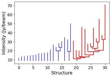
To determine the precise velocity range and extent of the gas associated with the Mystic Mountains complex, we use a dendrogram analysis to identify coherent structures in position-position-velocity space. As described in Rosolowsky et al. 2008 and Goodman et al. 2009, dendrograms provide a hierarchical representation of data, aiding the analysis of physical conditions on multiple scales from a single dataset. Large coherent features that are not part of another larger, parent structure are ‘trunks’; these contain substructures called ‘branches’ that are composed of individual local maxima, or ‘leaves,’ that cannot be subdivided further.
We use the python packages astrodendro (Robitaille et al. 2019) and scimes (Colombo et al. 2015) to decompose the structures in the CO datacube. We use the following parameters for the decomposition: a minimum value (min_value) that defines the noise threshold – we adopt 6; a minimum intensity (min_delta) for that defines the threshold the peak flux must exceed to be identified as a separate structure – we adopt 2; and a minimum number of pixels for a leaf to be an independent entity – we use the number equivalent to three beams (124 pixels in our case).
With these parameters, a dendrogram analysis identifies the Mystic Mountains as a trunk, indicating that it is a coherent cloud complex with contiguous emission over the velocity range km s-1. Figure 3 shows the Mystic Mountains as a single tree in red with other structures shown in blue. Within the Mystic Mountains complex, the dendrogram analysis identifies three separate pillars as branches. Contours defining the outlines of these branches are shown in Figure 4. We refer to the pillars by the name of the prominent jets that they host – HH 901, HH 902, and HH 1066.
In the following sections, we use this velocity range to derive the spatially-resolved physical parameters of the cold molecular gas in the Mystic Mountains. We provide maps of these spatially-resolved quantities in Appendix A and B. To provide representative values in Table 2, we compute the values within the dendrogram branches that define each of the pillars.


| Line | log(Nthin)max | log(Nthin)median | log(Nthick)peak | log(Nthick)median | |||
|---|---|---|---|---|---|---|---|
| [K km s-1] | [K km s-1] | [cm-2] | [cm-2] | [cm-2] | [cm-2] | ||
| Mystic Mountains; km s-1‡ | |||||||
| 12CO J=2-1 | 185.0 | 46.5 | 17.0 | 16.2 | 44.6 | 18.3 | 17.2 |
| 13CO J=2-1 | 57.5 | 8.8 | 16.5 | 15.4 | 4.2 | 16.6 | 15.5 |
| C18O J=2-1 | 6.9 | 1.14 | 15.6 | 14.8 | … | … | … |
| HH 901 pillar; km s-1† | |||||||
| 12CO J=2-1 | 114.2 | 38.8 | 16.8 | 16.4 | 33.0 | 18.0 | 17.5 |
| 13CO J=2-1 | 27.0 | 9.0 | 16.1 | 15.7 | 0.68 | 16.1 | 15.7 |
| C18O J=2-1 | 1.97 | 0.61 | 15.0 | 14.5 | … | … | … |
| HH 902 pillar; km s-1† | |||||||
| 12CO J=2-1 | 174.1 | 65.6 | 17.0 | 16.6 | 44.6 | 18.3 | 17.9 |
| 13CO J=2-1 | 56.8 | 18.3 | 16.5 | 16.0 | 1.9 | 16.6 | 16.0 |
| C18O J=2-1 | 6.90 | 1.84 | 15.6 | 15.0 | … | … | … |
| HH 1066 pillar; km s-1 | |||||||
| 12CO J=2-1 | 138.9 | 42.0 | 16.9 | 16.6 | 35.0 | 18.2 | 17.6 |
| 13CO J=2-1 | 42.1 | 7.65 | 16.4 | 15.7 | 3.1 | 16.4 | 15.8 |
| C18O J=2-1 | 4.03 | 0.81 | 15.3 | 14.7 | … | … | … |
| † from Cortes-Rangel et al. 2020 | |||||||
| ‡ from the intensity-weighted average velocity of the Mystic Mountains | |||||||
3.1 Optical depth
We compute the optical depth at each position and velocity where emission is detected with a significance using the following expression (Choi et al. 1993, equation 1 from):
| (1) |
where “main” is the more abundant species and “iso” is the optically thin (isotopologue) transition used to correct it. is the scale factor for the relative abundance of the two species. We use [12CO/13CO] (Rebolledo et al. 2016, see also Jacob et al. 2020) and [12CO/C18O] (Wilson & Rood 1994). We assume the same excitation temperature for both molecules. We find that CO emission is optically thick over a large portion of the Mystic Mountains whereas 13CO is only optically thick near the brightest emission in the HH 902 pillar. Maps of the spatially-resolved optical depth at the source velocity are shown in Appendix A and maximum values are reported in Table 2.
3.2 Molecular column density
We compute the column density of each observed transition using the following equation (Mangum & Shirley 2015, see e.g.,):
| (2) |
where is the rotational partition function for a given excitation temperature, is the rotational degeneracy of the upper level with energy , is the Einstein A coefficient for the transition, is the Boltzmann constant, is the Planck constant, is the Planck function in temperature units (K), and is a correction factor for non-zero optical depth (Goldsmith & Langer 1999, see, e.g.,). This assumes that all transitions have the same Tex. Physical parameters for the relevant molecules and transitions (frequency, rotational partition function, Einstein A coefficients, etc.) were obtained from the JPL Spectral Line Catalog (Pickett et al. 1998) and the Leiden Atomic and Molecular Database (Schöier et al. 2005, LAMBDA;).
To compute the column density, we assume an excitation temperature K. We assume that the gas temperature is the same as the dust temperature derived from the far-IR spectral energy distribution (SED) that Roccatagliata et al. 2013 used to compute a temperature map of the entire Carina region. As discussed in Mangum & Shirley 2015, assuming a single temperature is often a poor assumption and we expect that to be true for the Mystic Mountains. However, adopting higher excitation temperatures ( K) or a variable excitation temperature within this range changes the estimated column density by a factor of . In the absence of a better temperature measurement, we adopt a single number in this study. Maps of the spatially-resolved column density calculation for each of the CO isotopologues are shown in Appendix B and median column densities in each pillar are reported in Table 2.
3.3 Molecular gas mass of the Mystic Mountains
We estimate the mass of the Mystic Mountains complex from the optical-depth corrected spatially-resolved 2D CO column density map using the equation:
| (3) |
where (Pineda et al. 2010) is the abundance of H2 compared to CO, is the mean molecular weight (Kauffmann et al. 2008), is the mass of molecular hydrogen, and is the area of each pixel in the map. We compute a mass of 36 for the entire Mystic Mountains complex. More recent measurements find (Lacy et al. 2017) which reduce the estimated mass by a factor of 2.
3.4 Clumps, cores, and YSOs
3.4.1 C18O clumps


| Leaf | MM | R.A. | decl. | vsrc | M | Mvir | stable? | comment | |||
|---|---|---|---|---|---|---|---|---|---|---|---|
| (J2000) | (J2000) | [km s-1] | [pc] | [km s-1] | [km s-1] | [] | [] | ||||
| L1 | HH 1066 MM | 10:44:05.4 | 59:29:40 | -8.4 | 0.02 | 1.3 | 0.53 | 4.9 | 4.1 | N | |
| L2 | MM1 | 10:44:05.4 | 59:29:50 | -7.1 | 0.03 | 1.5 | 0.64 | 48.7 | 9.0 | N | 13CS |
| L3 | 10:44:05.2 | 59:29:56 | -7.0 | 0.02 | 1.3 | 0.52 | 5.6 | 4.5 | N | ||
| L4 | MM2 | 10:44:02.9 | 59:30:02 | -7.5 | 0.02 | 0.93 | 0.37 | 5.9 | 1.9 | N | |
| L5 | MM3 | 10:43:59.7 | 59:30:09 | -7.0 | 0.02 | 1.1 | 0.43 | 4.5 | 2.6 | N | |
| L6 | MM4 | 10:44:01.1 | 59:30:19 | -8.0 | 0.02 | 1.1 | 0.45 | 15.7 | 2.6 | N | DCN, 13CS |
| L7 | HH 902 MM | 10:44:01.7 | 59:30:27 | -7.8 | 0.02 | 1.2 | 0.50 | 17.8 | 3.3 | N | DCN, 2.7″ offset |
| L8 | MM5 | 10:44:05.3 | 59:30:20 | -5.1 | 0.01 | 1.1 | 0.46 | 3.5 | 3.0 | N | |
| L9 | 10:44:03.3 | 59:30:45 | -5.1 | 0.03 | 1.1 | 0.47 | 19.7 | 4.4 | N | ||
| L10 | HH 901 MM | 10:44:03.3 | 59:30:60 | -5.2 | 0.02 | 0.58 | 0.21 | 0.95 | 0.66 | N |
We repeat the dendrogram analysis on the C18O data to identify clumps using this higher density tracer. As for the CO analysis, we use the following thresholds: an intensity minimum value of 6 to ensure that we are using only well-detected emission, a minimum intensity of 2 to define a separate peak, and a minimum number of pixels equivalent to three beams. The leaves (local maxima) detected with this analysis are shown in Figure 5.
We extract the emission of the CO isotopologues within each C18O leaf (see Table 3) and plot the summed line profiles in Figure 6. In general, the most optically thick line, CO (shown with a solid line), has the broadest line profile. 13CO (dashed line) and C18O (dotted line) are each narrower, with some C18O profiles showing evidence of multiple velocity peaks. The three leaves associated with jet-driving sources are L1 (HH 1066), L7 (HH 902), and L10 (HH 901). L1 shows clear evidence of two distinct velocity components within the beam separated by km s-1. None of the three show evidence of red- and blue-shifted emission in the linewings that indicates an associated molecular outflow. These are likely washed out in the larger ACA beam as molecular outflows were detected in both HH 901 and HH 902 by Cortes-Rangel et al. 2020.


We use the median C18O line profile of each leaf to estimate its virial mass. We compute the virial mass using the following equation:
| (4) |
where is the exponent of the density profile (; we assume ), is the C18O linewidth (FWHM), is the mean leaf radius, and is the gravitational constant. Further corrections to account for the non-spherical morphologies will change these values by % (Bertoldi & McKee 1992). Virial masses, along with the linewidths, and 1D velocity dispersions for each leaf are reported in Table 3. We compare this to the molecular mass of each clump, computed as in Section 3.3 using using data from Wilson & Rood 1994 and Pineda et al. 2010. The molecular mass of all clumps is higher than their virial mass, suggesting that they unstable to collapse, as noted in Table 3.
3.4.2 Continuum sources


Figure 7 shows continuum emission detected with significance . This reveals 9 point sources. We detect continuum from clumps near the origin of all three of the famous HH jets in the Mystic Mountains – HH 901 MM, HH 902 MM, and HH 1066 MM. Five other continuum peaks fall within the Mystic Mountains (MM1-MM5); three of these reside in the HH 902 pillar (MM2-4; see Figure 7). The final point source, MM6, lies outside the Mystic Mountains complex so we do not discuss it further.
All mm continuum sources are associated with a C18O leaf, although not all C18O leaves have a continuum detection. Continuum and C18O emission are well-aligned spatially in all leaves but L7 at the head of the HH 902 pillar. Using a 2D Gaussian fit, we determine an offset of (0.03 pc) between the C18O and continuum peaks. The continuum peak is offset toward the western side of the pillar, in the same direction as the HH 902 YSO seen at higher resolution by Cortes-Rangel et al. 2020. A second continuum source detected to the northeast of the HH 902 YSO, HH 902 B, is not resolved with our larger beam.
Three additional continuum sources reside further north in the HH 902 pillar. A distinct peak in the continuum and C18O emission traces MM4 immediately to the north of the HH 902 MM. A bridge of continuum emission connects the two sources. Two additional continuum sources lie further north in the wishbone-shaped HH 902 pillar. MM2 and MM3 coincide with C18O peaks at the east and west tips of the pillar.
To the east of the HH 902 pillar, there are three continuum sources in the HH 1066 pillar. At the top (northernmost point) of the HH 1066 pillar is HH 1066 MM. Due south lies MM1. Like its neighbor, continuum and C18O emission from MM1 appear to peak behind a cloud edge traced by bright H emission. Further south, MM5 coincides with a C18O peak at the head of the HH 1066 pillar, adjacent to the continuum emission from the HH 902 MM and MM4.
Finally, at the tip of the Mystic Mountains complex, the HH 901 pillar has one continuum source detected at the head of the pillar. The continuum source overlaps with a local peak in the C18O emission. However, the brightest C18O emission in the HH 901 pillar is seen at its center where there is no continuum detection.
We compute masses of the continuum sources as:
| (5) |
We use a dust absorption coefficient = 0.8 cm2g-1 (Ossenkopf & Henning 1994) appropriate for 1.3 mm observations, and a temperature of T=30 K. We multiply the dust mass by a gas-to-dust ratio of 100 and report the total mass in Table 4. We have assumed a single temperature for all sources regardless of differences in their evolutionary stages (i.e., the presence of jets). Assuming a higher or lower temperature (15 K or 45 K) changes the estimated mass by a factor of . We refrain from a more detailed analysis given the low resolution of our data and evidence that multiple sources are unresolved in the beam (note that Cortes-Rangel et al. 2020, detect at least two point sources in the same region as our HH 902 MM). The flux and mass estimates of all continuum point sources are reported in Table 4.
| Source | R.A. | decl. | 225.9 GHz† | Mass |
| (J2000) | (J2000) | [mJy] | [] | |
| HH 1066 MM | 10:44:05.421 | 59:29:39.81 | 18.1 | 1.5 |
| HH 902 MM | 10:44:01.415 | 59:30:29.84 | 65.9 | 5.3 |
| HH 901 MM | 10:44:03.463 | 59:31:00.89 | 6.43 | 0.52 |
| MM1 | 10:44:05.327 | 59:29:50.65 | 13.3 | 1.1 |
| MM2 | 10:44:02.939 | 59:30:01.92 | 5.35 | 0.43 |
| MM3 | 10:43:59.146 | 59:30:02.95 | 6.25 | 0.51 |
| MM4 | 10:44:01.255 | 59:30:19.23 | 14.3 | 1.2 |
| MM5 | 10:44:05.503 | 59:30:22.43 | 4.76 | 0.39 |
| MM6 | 10:43:58.069 | 59:31:03.97 | 6.97 | 0.57 |
| †Aggregate continuum from the Band 6 observations. | ||||
3.4.3 Candidate YSOs detected in other surveys
Previous surveys at wavelengths 1.3 mm have also reported candidate YSOs in and around the Mystic Mountains. Three candidate YSOs from the Pan-Carina YSO Catalog (Povich et al. 2011, PCYC;) fall within the area of our ALMA map; these are shown on Figure 5 as black diamonds. All three candidate YSOs have an ambiguous evolutionary classification. PCYC 429 was identified as the HH 1066 driving source by Reiter et al. 2016 and coincides with the continuum source HH 1066 MM and the C18O emission of L1. Immediately below HH 1066 MM, a second candidate YSO, PCYC 427, lies near the northwest boundary of L2, outside the continuum emission of MM1. PCYC 427 coincides with a point source visible in H images suggesting that this source lies in front of the cloud. Further west, a third candidate YSO, PCYC 399, is also visible in H images. This source falls well outside the lowest contour of CO emission from the HH 902 pillar and has no associated continuum emission, suggesting that it is also lies outside the cloud.
Ohlendorf et al. 2012 searched for YSOs driving the prominent jets in the Mystic Mountains and other dust pillars in Carina. They note a point-like source near HH 902 that is not detected at longer (µm) wavelengths; this is shown as a cyan square in Figure 5. This source falls within HH 902 MM but is offset to the left, closer to the peak of the C18O emission. Coordinates reported by Ohlendorf et al. 2012 place the source away from the HH 902 YSO seen with ALMA by Cortes-Rangel et al. 2020. Together this suggests at least 3 YSOs unresolved in the HH 902 MM. Finally, no Herschel point sources were identified in the Mystic Mountains in the unbiased search by Gaczkowski et al. 2013.
3.5 Rarer species


Our observations included two rarer molecules, 13CS J=5-4 and DCN J=3-2. 13CS is a high-density tracer, typically seen in molecular envelopes and cavity walls (Tychoniec et al. 2021). DCN is most often observed in cold gas, where CO is frozen out of the enabling deuterium chemistry (Caselli & Ceccarelli 2012). Contour plots showing the emission peaks of both lines are presented in Figure 8 and Table 5. The strongest 13CS J=5-4 emission is associated with MM4. A second, weaker feature coincides with MM1.
DCN J=3-2 was serendipitously detected in a spectral window centered on SiO J=5-4; we do not detect SiO J=5-4 in any part of the mosaic. The brightest DCN peak is at the head of the HH 902 pillar, coincident with the HH 902 MM continuum source. Like the continuum emission, DCN is offset to the west of the C18O emission (see Figure 7).
DCN emission coincident with the HH 902 MM presents a double-peaked velocity profile, shown in Figure 9. The red peak is within km s-1 of the velocity peak of the C18O emission from the same region. The second peak is blueshifted by 1 km s-1. This velocity separation is not consistent with the frequency of any of the hyperfine components of DCN (Müller et al. 2001; Müller et al. 2005, using data from the Cologne Database for Molecular Spectroscopy; CDMS;). The flux of both peaks is remarkably similar, contrary to expectation for optically thin hyperfine emission. Finally, the velocity gradient is marginally resolved across the HH 902 MM (see Figure 9). Cortes-Rangel et al. 2020 observed a similar velocity gradient in N2D+ J=3-2 (note that their observations have better spatial resolution). Both deuterated molecules show a velocity gradient that is oriented opposite to the velocity structure of the HH 902 molecular outflow – that is, redshifted DCN (N2D+) is seen on the same side of the YSO as the blueshifted limb of the outflow.
A second, fainter DCN peak coincides with MM4. The emission peaks of all three molecules – DCN, 13CS, and C18O – coincide with continuum emission from MM4. Weak DCN emission extends from the position of MM2 along the edge of the pillar (see Figure 2).


| source | log(N)peak | log(N)median | ||
|---|---|---|---|---|
| [K km s-1] | [K km s-1] | |||
| DCN J=3-2 | ||||
| MM HH902 | 0.812 | 0.310 | 12.5 | 12.1 |
| MM 4 | 0.298 | 0.116 | 12.1 | 11.7 |
| 13CS J=5-4 | ||||
| MM 4 | 0.355 | 0.136 | 12.3 | 11.9 |
| MM 1 | 0.121 | 0.076 | 11.8 | 11.6 |
3.6 Velocity structure


Intensity-weighted velocity (moment 1) maps of the CO isotopologues are shown in Fig. 10. The most prominent feature is the velocity difference between the pillars of the Mystic Mountains. Some velocity differences are also apparent along the north/south axis of the HH 1066 pillar and the wishbone-like extensions of the HH 902 pillar. C18O emission suggests that there are multiple clumps in the HH 1066 pillar with slightly different velocities. Higher resolution observations are required to determine if the inter-clump gas is at a markedly different velocity, as seen in Pillar 6 of Klaassen et al. 2020.
3.7 Non-thermal motions
To test whether photoionization contributes to the non-thermal motions in the pillars, we compare the average velocity dispersion to the incident ionizing photon flux. To probe a larger range of fluxes, we compare the Mystic Mountains to the dust pillars in Carina from Klaassen et al. 2020 because those observations use the same angular resolution and spectral setup as this work. As in Klaassen et al. 2020, we compute the average velocity dispersion from the moment 2 map. We consider the Mystic Mountains as a whole and each of the three pillars within it separately. To calculate the incident ionizing photon flux, we assume that the three main star clusters, Tr14, Tr15, and Tr16, dominate the external irradiation for all pillars in Carina. This provides a lower bound as we neglect the large number of O- and B-type stars located outside these clusters (Berlanas et al. 2023, see, e.g.,) and the effects of extinction. We use the ionizing photon luminosities from Smith 2006a and compute the local flux using the projected distance between the pillars and the clusters22 2 The nearest cluster in projection does not always dominate the ionization. For example, Pillar 20 lies alongside Tr15 but points toward Tr16, suggesting that it has had a stronger influence. . The mean pillar velocity dispersion as a function of incident ionizing photon flux is shown in Figure 11 (color-coded by whether the pillars contain a jet seen at visual wavelengths, see discussion in Section 4.1).

Within the (large) uncertainties, the mean velocity dispersions are similar across nearly two orders of magnitude in incident ionizing radiation. This is counter to expectation if ionizing radiation drives turbulence in the gas. However, moment 2 maps do not isolate non-thermal motions from other factors that contribute to the linewidth. Bulk motions from large-scale processes like infall and rotation as well as the influence of outflows from protostars embedded in the pillars will all contribute to this single value. In addition, higher temperatures will increase the thermal contribution to the linewidth. However, to first order we would expect pillars subject to higher ionizing photon fluxes would also have warmer temperatures (Roccatagliata et al. 2013; Rebolledo et al. 2016, see, e.g., the dust temperature maps from).
For the Mystic Mountains we separate thermal and turbulent motions as follows. We use the linewidth measured as the full width at half maximum (FWHM; ) to calculate the 1D velocity dispersion, . To compute the thermal contribution, we use where is the mass of the CO isotopologue used and T=30 K is the temperature of the cold molecular gas. Subtracting the thermal component from the total velocity dispersion yields the 1D turbulent velocity dispersion, . Finally, we convert the 1D estimate to 3D as . The 3D turbulent velocity dispersion computed for each CO isotopologue is shown in Figure 12.


Velocity dispersions are higher in CO than in 13CO and C18O. The highest values for the turbulent velocity dispersion are observed where the pillars overlap, almost certainly reflecting the influence of multiple velocity components along the line of sight. Other regions with high values of the velocity dispersion fall behind ionization fronts traced by H (see Figure 13).
The HH 902 pillar is well resolved with our 6″ beam and overlaps only minimally with the other pillars in the Mystic Mountains. Qualitatively, the velocity dispersion is higher where the H emission is higher. Velocity dispersions are larger along the western edge of the pillar and modest peaks appear behind the two H ridges at the head of the pillar. Peaks in the velocity dispersion do not coincide with the location of the continuum sources.
When estimating , we assumed a single temperature of T=30 K for the entire Mystic Mountains. Gas temperatures are likely higher in the most heavily irradiated parts of the Mystic Mountains. Assuming a higher temperature, T=50 K, yields a larger thermal contribution km s-1 which is roughly equivalent to the average velocity dispersion of the Mystic Mountains (as estimated from the moment 2 map).


In addition to temperature uncertainties, the lack of correlation between velocity dispersion and incident ionizing photon flux may result from one of the following possibilities: (1) turbulence is enhanced only near irradiated cloud surfaces in layers too thin to be resolved with our 6″ beam; (2) different pillars have a different level of embedded star formation that contributes unequally to the observed linewidth (i.e. via outflows) but is unresolved in our beam (and star formation activity itself does not vary as a function of incident ionizing flux); or (3) that ionizing radiation does not drive turbulence.
However, the velocity dispersion may not be best discriminant of the impact of ionizing radiation on the gas. External radiation may drive non-thermal motions through compressive shocks but shock energy will quickly dissipate and the velocity signature may not be long-lived. Compressive motions will also reshape the density of the gas, leaving behind local regions of higher density. We consider this signature of compressive turbulence in the next section.
3.8 Isolating turbulent motions
Menon et al. 2021 used the data of Klaassen et al. 2020 to measure the turbulence in a few well-resolved pillars.
They reconstruct the dominant turbulence driving mode from the column density and intensity-weighted velocity maps (Federrath et al. 2010; Federrath
et al. 2016).
In this section, we repeat this analysis for the Mystic Mountains complex for a highly irradiated comparison.
2D density structure: To compute the density probability distribution function (PDF), we use the column density of the optically thin 13CO as a proxy for the H2 along the line of sight, , substituting the C18O in places where the 13CO is optically thick. We compute , the dispersion of the natural logarithm of the column density scaled by its mean () by fitting a Hopkins 2013 intermittency density PDF model to the volume-weighted PDF of . This has the form
| (6) |
where
| (7) |
and
| (8) |
and is the intermittency parameter. The values of and derived from the fit are used to compute , the linear dispersion, as
| (9) |
using an expression from Hopkins 2013.
Conversion from 2D to 3D density structure: We estimate the 3D density dispersion from the 2D column density dispersion using the method of Brunt et al. 2010. The 3D density power spectrum, P, of the variable is reconstructed from the 2D column density power spectrum, P, of the variable ; is the wavenumber. This is converted to the 3D power spectrum as P. The ratio of the 2D and 3D dispersions is defined as
| (10) |
where we have mirrored the column density to provide a periodic dataset (Ossenkopf et al. 2008).
Isolating turbulent motions: We fit a plane to the intensity-weighted velocity map (the first moment map) to remove bulk motions and isolate turbulent motions in the pillars. For purely turbulent motion, we expect the line of sight motions to trace a Gaussian PDF. We fit a Gaussian to the line of sight velocity PDF to derive the 1D velocity dispersion, . We convert this to the 3D velocity dispersion as , implicitly assuming isotropy.
From this, we compute the Mach number, , which is the ratio of the 3D velocity dispersion and the sound speed, km s-1 for our assumed temperature of 30 K. Finally, we compute , the turbulence driving parameter as . The value of is used to determine the type of turbulence: is purely solenoidal; is purely compressive; and is a combination of both.
Values of each of the derived parameters and their 1 uncertainties
are listed in Table 6.
PDFs of the column density and velocities for the Mystic Mountains are shown in Figure 14.
We focus our comparison on the Mystic Mountains as a whole because the individual pillars are significantly smaller, with only a few beams covering their major and minor axes.
Results of this analysis for each individual pillar are shown in Appendix C but we do not discuss them further here as the individual pillars are inadequately resolved for this analysis
(similar to Pillar 44 in Menon et al. 2021; see also Sharda et al. 2018).
Comparing the Mystic Mountains to other pillars in Carina: Within the Mystic Mountains, it is clear that there are multiple velocity components; these roughly correspond to the systemic velocity of each pillar (see Figure 14 and Table 2). Subtracting a linear function (a plane) reduces the peakiness of the velocity distribution, but the velocity dispersion remains large even after gradient subtraction, nearly a factor of two higher than the values found by Menon et al. 2021 for other pillars in Carina. As a result, the Mach number () is also a factor of 2 higher. The resulting turbulence driving parameter b is within the range of compressively-dominated turbulence () but somewhat lower than the values () found by Menon et al. 2021.
| Pillar | MM |
|---|---|
| A [pc2] | 0.32 |
| [1021 cm-2] | 3.01 |
| [] | 33.7 |
| n [cm-3] | 2.33 |
| [km s-1] | 0.34 |
| 26.7 | |
| tff/tturb | 2.22 |
| 1.01 | |
| 0.56 | |
| 0.14 | |
| 4.02 | |
| [km s-1] | 1.76 |
| [km s-1] | 1.26 |
| [km s-1] | 2.19 |
| 7.29 | |
| 0.55 |


4 Discussion
Recent numerical work suggests that ionizing radiation may drive turbulence in cold molecular gas via the rocket effect (Gritschneder et al. 2009; Boneberg et al. 2015; Dale 2017; Menon et al. 2020, e.g.,). Photoevaporation drives a flow of free electrons from ionized cloud surfaces. Momentum is conserved, so this flow also drives a shock into the cloud, compressing the gas and perhaps injecting turbulence.
In this picture, highly irradiated pillars like the Mystic Mountains should show a high level of turbulent velocity dispersion in the gas. The Mystic Mountains cloud complex lies in the heart of the Carina Nebula where copious ionizing photons from Tr14 (Smith 2006a, s-1, see) illuminate and sculpt its mountainous morphology. The incident ionizing photon flux illuminating the Mystic Mountains is an order of magnitude higher than that illuminating other pillars in Carina with similar observations (Klaassen et al. 2020, see Figure 11 and).
A clear correlation between the incident ionizing radiation and electron density in ionization fronts has been observed in dust pillars in Carina (McLeod et al. 2016). We do not find a similarly straight-forward relationship between the cold molecular gas and incident radiation. Despite the higher ionizing flux illuminating the Mystic Mountains, the average velocity dispersion (derived from the moment 2 map) is comparable to other pillars in Carina (see Figure 11). At , the turbulence driving parameter is consistent with compressive turbulence but is below the range found by Menon et al. 2021.
For all of the pillars in Carina that have been observed with the ACA alone, it is unclear what role unresolved star formation activity plays in the observed kinematics. In the Mystic Mountains, we detect 8 continuum sources (see Section 3.4.2) and 10 C18O clumps (see Section 3.4). The pillars in the Klaassen et al. 2020 also display a wide range of star-formation activity from the relatively quiescent Pillar 22 which has only two C18O cores to the actively star-forming Pillar 6 with evidence for 4 separate YSOs. Protostars and their (unresolved) outflows can contribute to internal velocity dispersion (Larson et al. 2015, e.g.,) and may provide a local source of turbulence. Quantifying this is difficult, however, as we do not detect the known outflows in the Mystic Mountains or any other molecular outflows, likely due to the modest resolution of our data (at 2.3 kpc, our ″ beam corresponds to 0.07 pc). The physical properties of the famous jets in the Mystic Mountains (see Figure 1) are well measured (Reiter & Smith 2013; Reiter & Smith 2014; Cortes-Rangel et al. 2020) but these largely propagate outside the cloud.
Higher angular resolution observations are required to detect and remove the influence of embedded outflows as well as analyze the individual pillars of the Mystic Mountains independently. Existing data covers a small region at the head of the HH 901 and HH 902 pillars (Cortes-Rangel et al. 2020); extending this to a larger portion of the Mystic Mountains would be interesting to do in the future. For now, we compare the results of the Mystic Mountains and the Klaassen et al. 2020 pillars to higher resolution observations of other portions of the Carina region.
4.1 Comparison to other regions in Carina
A few other studies in the Carina region have quantified the impact of ionizing feedback on star-forming gas. Rebolledo et al. 2020 compared two clouds in the Carina region that are subject to very different ionizing radiation fields: the ‘North Cloud’ which is located near the center of Carina where it is heavily irradiated by Tr14 and the ‘South Pillars’ regions which is located in the outskirts of Carina where it is subject to much less intense radiation. The two regions are separated from the central clusters, Tr14 and Tr16, by 2.5 pc and 30 pc, respectively, and thus experience an order of magnitude difference in their radiative environment. With Band 3 observations targeting the dense gas tracers HCN and HCO+ with a resolution of , Rebolledo et al. 2020 find evidence for more turbulence in the heavily irradiated North Cloud. The North Cloud also has fewer cores than the South Pillars region. However, the cores that have formed in the North Cloud are higher in mass than the more numerous cores found in the South Pillars cloud, consistent with turbulent fragmentation.
Hartigan et al. 2022 recently published observations of the ‘Western Wall,’ a region in the center of Carina that overlaps with the North Cloud from Rebolledo et al. 2020. These higher resolution observations (synthesized beamsize ) in Band 6 target CO and its isotopologues. Hartigan et al. 2022 conclude that the influence of feedback is modest with no signs of triggered star formation and no prominent dust pillars. Gas densities appear higher immediately behind the ionization front but cores appear starless, and there is no evidence for grain growth. A follow-up analysis of the Hartigan et al. 2022 observations from Downes et al. 2023 determined that turbulence is driven at large scales, but not necessarily by irradiation from nearby high-mass stars.
This conclusions stands in contrast to Menon et al. 2021 who argue that predominantly compressive modes of turbulence may have triggered star formation in the pillars. However, Downes et al. 2023 argue that their result is not in tension with Menon et al. 2021. Unlike the Western Wall, the pillars have been sculpted by radiation. Pillars may self-shadow, allowing compressive motions to lead to their development, altering their internal kinematics.
In the simulations of Dale et al. 2012, prominent pillars form in clouds with more diffuse gas and those with smoother density fields. Above a certain density (100 cm-3), ionization is dynamically ineffective, especially in more turbulent regions. On the smaller scales of the pointed observations presented in this paper and those in Klaassen et al. 2020, Rebolledo et al. 2020, and Hartigan et al. 2022, differences in the local initial conditions may be responsible for the morphological differences observed at present. In this case, ionizing radiation carved more diffuse gas into dust pillars, perhaps triggering star formation (Brooks et al. 2002; Rathborne et al. 2004; Smith et al. 2010b; Ohlendorf et al. 2012). Meanwhile, the higher density Western Wall / North Cloud began as and remained a higher density region (Rebolledo et al. 2020, see, e.g., Figure 1 in), less vulnerable to compression. Local density variations may also help explain why there is a dust pillar 1′ (0.7 pc) to the northeast of the Western Wall (Smith et al. 2010a, see).
This picture is in line with the simulations of Tremblin et al. 2012a; Tremblin et al. 2012b who find that pillar formation depends strongly on shock curvature. Pre-existing overdensities help curve the shock driven by the ionization front. Pillars form when the curved shock collapses in on itself. Pillars formed in this way will naturally have a high-density core at their tips in much the same way that desert buttes have high-density caprock at their apices.
While differences in the initial density may help explain the absence of pillars in the Western Wall, the low level of star formation activity remains a challenge. High initial densities in the Western Wall suggest that star formation would happen sooner than in the feedback-carved pillars. But this is not what is observed. Hartigan et al. 2022 find that the cores in the Western Wall are starless. Rebolledo et al. 2020 argue that the higher level of turbulence may have made the Western Wall more resilient to fragmentation as there are fewer but higher mass cores compared to their more quiescent South Pillars region. In contrast, several pillars show evidence for star formation in the form of their prominent jets.
Turbulence rapidly decays and must be constantly resupplied to maintain observed levels. Rebolledo et al. 2020 attribute the higher turbulence in the North Cloud / Western Wall to the impact of external irradiation. Downes et al. 2023 also find evidence that turbulence is driven on large scales, but they do not attribute this to ionization. Resolving this tension requires a more homogeneous dataset that covers the large (pc) scales where turbulence is driven while resolving the 0.02 pc – 0.03 pc scales that Downes et al. 2023 find are also dynamically important.
5 Conclusions
In this paper, we present maps of the CO, 13CO, and C18O emission from the Mystic Mountains, a large cloud complex with multiple dust pillars located in the heart of the Carina Nebula. A dendrogram analysis reveals a coherent, connected structure with three individual pillars. We detect eight continuum cores within the Mystic Mountains. Most continuum cores are associated with a C18O clump, but not all C18O clumps have a continuum counterpart. The rarer isotopologues DCN J=3-2 and 13CS J=5-4 are detected in two clumps located in the region with the highest column density.
The Mystic Mountains region experiences an order of magnitude higher ionizing flux from the nearby star clusters than the flux incident on other dust pillars in Carina observed with similar tracers and angular resolution. However, bulk pillar properties like the average velocity dispersion derived from moment 2 maps are similar for all pillars, regardless of their irradiation.
A more detailed analysis to isolate turbulent motions reveals a turbulent driving parameter, , consistent with compressive turbulence dominating in the Mystic Mountains. The derived is within the range of values found by Menon et al. 2021 for the pillars from Klaassen et al. 2020. The derived Mach number for the Mystic Mountains is a factor of 2 higher than that found for other pillars in the Carina region, either reflecting a stronger shock from the more intense UV field, or, more likely, is artificially inflated by the broad velocity distribution of the Mystic Mountains.
The similarity of pillar properties across a range of incident ionizing fluxes contrasts with studies of other irradiated clouds in the Carina Nebula. Rebolledo et al. 2020 compared two regions with an order of magnitude difference in the incident radiation and find evidence for more turbulence and fewer (but higher mass) cores in the more heavily irradiated cloud. From a different analysis and dataset of the same region presented by Rebolledo et al. 2020, Downes et al. 2023 argue that differences between the pillar results and the cloud results are not inconsistent because pillar kinematics may reflect dynamical compression. We argue that this may be true if the different morphologies observed today result from different initial densities that aided or prevented UV irradiation from compressing the local cloud into a pillar. Pre-existing overdensities may also explain the observed difference in star-forming activity. Cores in the Western Wall / North Cloud appear starless whereas a fraction of the cores in the Mystic Mountains and other pillars drive prominent jets, signifying a more advanced evolutionary stage (Cortes-Rangel et al. 2020, i.e. HH 901 and HH 902 in the Mystic Mountains; see).
Future work probing a broader range of environments with the angular resolution to probe both the large scales of turbulence driving and the small scales where its consequences are most evident will help resolve this tension.
Acknowledgements
We would like to thank the referee, Neal Evans, for a prompt and thoughtful report that improved the manuscript. We would like to thank Shyam Menon for a careful reading of the manuscript and thoughtful feedback. MR was partially supported by an ESO fellowship. DI was funded by the European Research Council (ERC) via the ERC Synergy Grant ECOGAL (grant 855130). This paper makes use of the following ALMA data: ADS/JAO.ALMA#2018.1.01001.S. ALMA is a partnership of ESO (representing its member states), NSF (USA) and NINS (Japan), together with NRC (Canada) and NSC and ASIAA (Taiwan) and KASI (Republic of Korea), in cooperation with the Republic of Chile. The Joint ALMA Observatory is operated by ESO, AUI/NRAO and NAOJ. The National Radio Astronomy Observatory is a facility of the National Science Foundation operated under cooperative agreement by Associated Universities, Inc. This work uses observations made with the NASA/ESA Hubble Space Telescope, obtained from the Data Archive at the Space Telescope Science Institute, which is operated by the Association of Universities for Research in Astronomy, Inc., under NASA contract NAS 5-26555. The HST observations are associated with GO-12050. This research made use of Astropy33 3 http://www.astropy.org, a community developed core Python package for Astronomy (Astropy Collaboration et al. 2013; Price-Whelan et al. 2018). This research made use of APLpy, an open-source plotting package for Python (Robitaille & Bressert 2012). This research made use of the following software packages: astrodendro, a Python package to compute dendrograms of Astronomical data (http://www.dendrograms.org/); SCIMES, a Python package to find relevant structures into dendrograms of molecular gas emission using the spectral clustering approach (Colombo et al. 2015); and TurbuStat, a Python package to compute 14 turbulence-based statistics described in the astronomical literature (Koch et al. 2017; Koch et al. 2019).
Data Availability
The ALMA data used in this study are publicly available from the ALMA archive 44 4 https://almascience.nrao.edu/aq/?result_view=observations under the program ID number ADS/JAO.ALMA#2018.1.01001.S. Data from HST are publicly available via the MAST archive55 5 https://mast.stsci.edu/portal/Mashup/Clients/Mast/Portal.html.
References
- Astropy Collaboration et al. (2013) Astropy Collaboration et al., 2013, aap, 558, A33
- Berlanas et al. (2023) Berlanas S. R., et al., 2023, A&A, 671, A20
- Bertoldi (1989) Bertoldi F., 1989, ApJ, 346, 735
- Bertoldi & McKee (1992) Bertoldi F., McKee C. F., 1992, ApJ, 395, 140
- Boneberg et al. (2015) Boneberg D. M., Dale J. E., Girichidis P., Ercolano B., 2015, MNRAS, 447, 1341
- Brooks et al. (2002) Brooks K. J., Rathborne J. M., Burton M. G., Cox P., 2002, in Crowther P., ed., Astronomical Society of the Pacific Conference Series Vol. 267, Hot Star Workshop III: The Earliest Phases of Massive Star Birth. p. 353 (arXiv:astro-ph/0108519), doi:10.48550/arXiv.astro-ph/0108519
- Brunt et al. (2010) Brunt C. M., Federrath C., Price D. J., 2010, MNRAS, 403, 1507
- Caselli & Ceccarelli (2012) Caselli P., Ceccarelli C., 2012, A&ARv, 20, 56
- Chevance et al. (2022) Chevance M., et al., 2022, MNRAS, 509, 272
- Choi et al. (1993) Choi M., Evans Neal J. I., Jaffe D. T., 1993, ApJ, 417, 624
- Colombo et al. (2015) Colombo D., Rosolowsky E., Ginsburg A., Duarte-Cabral A., Hughes A., 2015, MNRAS, 454, 2067
- Cortes-Rangel et al. (2020) Cortes-Rangel G., Zapata L. A., Toalá J. A., Ho P. T. P., Takahashi S., Mesa-Delgado A., Masqué J. M., 2020, AJ, 159, 62
- Dale (2017) Dale J. E., 2017, MNRAS, 467, 1067
- Dale et al. (2012) Dale J. E., Ercolano B., Bonnell I. A., 2012, MNRAS, 424, 377
- Downes et al. (2023) Downes T. P., Hartigan P., Isella A., 2023, MNRAS, 519, 5427
- Elmegreen & Lada (1977) Elmegreen B. G., Lada C. J., 1977, ApJ, 214, 725
- Federrath et al. (2010) Federrath C., Roman-Duval J., Klessen R. S., Schmidt W., Mac Low M. M., 2010, A&A, 512, A81
- Federrath et al. (2016) Federrath C., et al., 2016, ApJ, 832, 143
- Gaczkowski et al. (2013) Gaczkowski B., Preibisch T., Ratzka T., Roccatagliata V., Ohlendorf H., Zinnecker H., 2013, A&A, 549, A67
- Goldsmith & Langer (1999) Goldsmith P. F., Langer W. D., 1999, ApJ, 517, 209
- Goodman et al. (2009) Goodman A. A., Pineda J. E., Schnee S. L., 2009, ApJ, 692, 91
- Göppl & Preibisch (2022) Göppl C., Preibisch T., 2022, A&A, 660, A11
- Gritschneder et al. (2009) Gritschneder M., Naab T., Walch S., Burkert A., Heitsch F., 2009, ApJ, 694, L26
- Gritschneder et al. (2010) Gritschneder M., Burkert A., Naab T., Walch S., 2010, ApJ, 723, 971
- Hartigan et al. (2015) Hartigan P., Reiter M., Smith N., Bally J., 2015, AJ, 149, 101
- Hartigan et al. (2022) Hartigan P., Hummel M., Isella A., Downes T., 2022, arXiv e-prints, p. arXiv:2209.10013
- Hester et al. (1996) Hester J. J., et al., 1996, AJ, 111, 2349
- Hopkins (2013) Hopkins P. F., 2013, MNRAS, 430, 1880
- Jacob et al. (2020) Jacob A. M., Menten K. M., Wiesemeyer H., Güsten R., Wyrowski F., Klein B., 2020, A&A, 640, A125
- Kauffmann et al. (2008) Kauffmann J., Bertoldi F., Bourke T. L., Evans N. J. I., Lee C. W., 2008, A&A, 487, 993
- Klaassen et al. (2014) Klaassen P. D., Mottram J. C., Dale J. E., Juhasz A., 2014, MNRAS, 441, 656
- Klaassen et al. (2020) Klaassen P. D., Reiter M. R., McLeod A. F., Mottram J. C., Dale J. E., Gritschneder M., 2020, MNRAS, 491, 178
- Koch et al. (2017) Koch E. W., Ward C. G., Offner S., Loeppky J. L., Rosolowsky E. W., 2017, MNRAS, 471, 1506
- Koch et al. (2019) Koch E. W., Rosolowsky E. W., Boyden R. D., Burkhart B., Ginsburg A., Loeppky J. L., Offner S. S. R., 2019, AJ, 158, 1
- Kruijssen et al. (2019) Kruijssen J. M. D., et al., 2019, Nature, 569, 519
- Lacy et al. (2017) Lacy J. H., Sneden C., Kim H., Jaffe D. T., 2017, ApJ, 838, 66
- Larson et al. (2015) Larson R. L., Evans Neal J. I., Green J. D., Yang Y.-L., 2015, ApJ, 806, 70
- Mangum & Shirley (2015) Mangum J. G., Shirley Y. L., 2015, PASP, 127, 266
- Matzner (2002) Matzner C. D., 2002, ApJ, 566, 302
- McLeod et al. (2016) McLeod A. F., et al., 2016, MNRAS, 462, 3537
- McLeod et al. (2021) McLeod A. F., et al., 2021, MNRAS, 508, 5425
- McMullin et al. (2007) McMullin J. P., Waters B., Schiebel D., Young W., Golap K., 2007, in Shaw R. A., Hill F., Bell D. J., eds, Astronomical Society of the Pacific Conference Series Vol. 376, Astronomical Data Analysis Software and Systems XVI. p. 127
- Menon et al. (2020) Menon S. H., Federrath C., Kuiper R., 2020, MNRAS, 493, 4643
- Menon et al. (2021) Menon S. H., Federrath C., Klaassen P., Kuiper R., Reiter M., 2021, MNRAS, 500, 1721
- Mesa-Delgado et al. (2016) Mesa-Delgado A., Zapata L., Henney W. J., Puzia T. H., Tsamis Y. G., 2016, ApJ, 825, L16
- Müller et al. (2001) Müller H. S. P., Thorwirth S., Roth D. A., Winnewisser G., 2001, A&A, 370, L49
- Müller et al. (2005) Müller H. S. P., Schlöder F., Stutzki J., Winnewisser G., 2005, Journal of Molecular Structure, 742, 215
- Ohlendorf et al. (2012) Ohlendorf H., Preibisch T., Gaczkowski B., Ratzka T., Grellmann R., McLeod A. F., 2012, A&A, 540, A81
- Ossenkopf & Henning (1994) Ossenkopf V., Henning T., 1994, A&A, 291, 943
- Ossenkopf et al. (2008) Ossenkopf V., Krips M., Stutzki J., 2008, A&A, 485, 917
- Pickett et al. (1998) Pickett H. M., Poynter R. L., Cohen E. A., Delitsky M. L., Pearson J. C., Müller H. S. P., 1998, J. Quant. Spectrosc. Radiative Transfer, 60, 883
- Pineda et al. (2010) Pineda J. L., Goldsmith P. F., Chapman N., Snell R. L., Li D., Cambrésy L., Brunt C., 2010, ApJ, 721, 686
- Povich et al. (2011) Povich M. S., et al., 2011, ApJS, 194, 14
- Price-Whelan et al. (2018) Price-Whelan A. M., et al., 2018, aj, 156, 123
- Rathborne et al. (2004) Rathborne J. M., Brooks K. J., Burton M. G., Cohen M., Bontemps S., 2004, A&A, 418, 563
- Rebolledo et al. (2016) Rebolledo D., et al., 2016, MNRAS, 456, 2406
- Rebolledo et al. (2020) Rebolledo D., et al., 2020, ApJ, 891, 113
- Reiter & Smith (2013) Reiter M., Smith N., 2013, MNRAS, 433, 2226
- Reiter & Smith (2014) Reiter M., Smith N., 2014, MNRAS, 445, 3939
- Reiter et al. (2016) Reiter M., Smith N., Bally J., 2016, MNRAS, 463, 4344
- Reiter et al. (2017) Reiter M., Kiminki M. M., Smith N., Bally J., 2017, MNRAS, 470, 4671
- Robitaille & Bressert (2012) Robitaille T., Bressert E., 2012, APLpy: Astronomical Plotting Library in Python, Astrophysics Source Code Library (ascl:1208.017)
- Robitaille et al. (2019) Robitaille T., Rice T., Beaumont C., Ginsburg A., MacDonald B., Rosolowsky E., 2019, astrodendro: Astronomical data dendrogram creator, Astrophysics Source Code Library, record ascl:1907.016 (ascl:1907.016)
- Roccatagliata et al. (2013) Roccatagliata V., Preibisch T., Ratzka T., Gaczkowski B., 2013, A&A, 554, A6
- Rosolowsky et al. (2008) Rosolowsky E. W., Pineda J. E., Kauffmann J., Goodman A. A., 2008, ApJ, 679, 1338
- Schneider et al. (2012) Schneider N., et al., 2012, A&A, 542, L18
- Schöier et al. (2005) Schöier F. L., van der Tak F. F. S., van Dishoeck E. F., Black J. H., 2005, A&A, 432, 369
- Sharda et al. (2018) Sharda P., Federrath C., da Cunha E., Swinbank A. M., Dye S., 2018, MNRAS, 477, 4380
- Smith (2006a) Smith N., 2006a, MNRAS, 367, 763
- Smith (2006b) Smith N., 2006b, ApJ, 644, 1151
- Smith et al. (2010a) Smith N., Bally J., Walborn N. R., 2010a, MNRAS, 405, 1153
- Smith et al. (2010b) Smith N., et al., 2010b, MNRAS, 406, 952
- Tremblin et al. (2012a) Tremblin P., Audit E., Minier V., Schneider N., 2012a, A&A, 538, A31
- Tremblin et al. (2012b) Tremblin P., Audit E., Minier V., Schmidt W., Schneider N., 2012b, A&A, 546, A33
- Tremblin et al. (2013) Tremblin P., et al., 2013, A&A, 560, A19
- Tychoniec et al. (2021) Tychoniec Ł., et al., 2021, A&A, 655, A65
- Walch et al. (2013) Walch S., Whitworth A. P., Bisbas T. G., Wünsch R., Hubber D. A., 2013, MNRAS, 435, 917
- Wilson & Rood (1994) Wilson T. L., Rood R., 1994, ARA&A, 32, 191
Appendix A Optical depth maps
Maps of the average and maximum 12CO optical depth are shown in Figure 15. The median value for the Mystic Mountains and each individual pillar are reported in Table 2.


Appendix B Column density maps
The spatially-resolved, optical-depth corrected column density of each of the three CO isotopologues is shown in Figure 16. Peak and median values for the Mystic Mountains and each individual pillar are reported in Table 2.


Appendix C Turbulence Driving Parameter analysis for the individual pillars
We repeat the analysis in Section 3.8 to isolate turbulent motions in each pillar of the Mystic Mountains complex individually. The pillars in the Mystic Mountains are all at slightly different velocities and these differences are not cleanly removed with a linear gradient. These real velocity differences therefore inflate any measure of the velocity dispersion for the Mystic Mountains as a whole. Ideally, each pillar would be analyzed separately to remove these systematic motions.
Figures 17, 18, and 19 show the results of this analysis for the individual pillars and Table 7 reports the derived values with 1 uncertainties. We find unphysical values for many parameters, including the turbulent driving parameter . This is almost certainly a reflection of the low resolution of our data compared to the size of the pillars: the width of the HH 901 and HH 1066 pillars are both comparable to the size of the beam.
To test this, we degraded the resolution of the data to 1/4 of the native resolution (Sharda et al. 2018, as in). Repeating the analysis, we find that changes by 20% for the separate pillars. For the Mystic Mountains as a whole, derived values change by 6% using the lower-resolution data. Formal error propagation does not capture this underlying problem, leading to modest uncertainties on unphysical values in Table 7. A more reliable analysis requires higher angular observations that better resolve the individual pillars.


| Pillar | HH 901 | HH 902 | HH 1066 |
|---|---|---|---|
| A [pc2] | 0.070.007 | 0.180.02 | 0.200.02 |
| [1021 cm-2] | 3.09 | 7.59 | 3.47 |
| [] | 3.312.64 | 17.213.2 | 8.137.51 |
| n [cm-3] | 4.161.06 | 6.100.76 | 2.950.80 |
| [km s-1] | 0.310.23 | 0.270.15 | 0.260.26 |
| 16.31.90 | 0.760.12 | 1.240.33 | |
| tff/tturb | 1.730.10 | 0.370.03 | 0.480.06 |
| 0.99 | 0.63 | 0.67 | |
| 0.52 | 0.46 | 0.45 | |
| 0.09 | 0.13 | 0.09 | |
| 5.760.21 | 3.49.15 | 4.75.08 | |
| [km s-1] | 0.910.20 | 0.320.02 | 1.310.26 |
| [km s-1] | 0.620.07 | 0.250.01 | 0.240.01 |
| [km s-1] | 1.070.13 | 0.440.02 | 0.410.02 |
| 3.580.43 | 1.470.05 | 1.380.07 | |
| 1.610.2 | 2.370.13 | 3.450.19 |
