‡UCSD †NVIDIA
CleanUNet 2: A Hybrid Speech Denoising Model on
Waveform and Spectrogram
Abstract
In this work, we present CleanUNet 2, a speech denoising model that combines the advantages of waveform denoiser and spectrogram denoiser and achieves the best of both worlds. CleanUNet 2 uses a two-stage framework inspired by popular speech synthesis methods that consist of a waveform model and a spectrogram model. Specifically, CleanUNet 2 builds upon CleanUNet, the state-of-the-art waveform denoiser, and further boosts its performance by taking predicted spectrograms from a spectrogram denoiser as the input. We demonstrate that CleanUNet 2 outperforms previous methods in terms of various objective and subjective evaluations. 11 1 Audio samples: https://cleanunet2.github.io/
Index Terms: speech denoising, speech enhancement
1 Introduction
Speech recorded in real world scenarios may contain various background noise. Examples are audio-video conferences, automatic speech recognition, and hearing aids. To tackle this problem, speech denoising techniques [1] aim to remove such noise and then output perceptually high-quality speech signals.
Speech denoising methods have been studied for decades, ranging from traditional signal processing methods [2, 3] to machine learning methods [4, 5]. In recent years, deep neural networks [6, 7] have achieved state-of-the-art (SOTA) results because of large model capacity to process large-scale training data [8]. In these models, speech denoising is usually considered as a regression task: the networks are trained to directly predict clean speech given noisy speech as inputs. These models mainly fall into two categories: spectrogram-based methods and waveform-based methods.
Most speech denoising methods are spectrogram-based [7, 9, 10, 11, 12, 13, 14, 15, 16, 17, 18, 19]. These methods first extract noisy spectral feature (such as magnitude of spectrogram or complex spectrum). Then, they predict a mask for modulation (e.g., the ideal ratio mask [20]) or the spectral feature of clean speech. The final step is to generate waveform based on the predicted mask or spectral feature with other information (such as phase) extracted from the noisy speech. These methods work well under moderate noise levels, but will have noticeable noise leakage under high noise levels mostly due to inaccurate phase estimation from noisy speech.
Waveform-based methods, in contrast, directly predict the waveform representation of clean speech from the noisy waveform [21, 22, 23, 24, 25, 26, 27]. Most waveform-based methods use WaveNet [28] or U-Net [29] as backbone, with different sub-modules such as dilated convolutions [30, 25], stand-alone WaveNet [24], LSTM [26], and self-attention [31, 27]. The state-of-the-art waveform-based methods are able to prevent noise leakage well even under high noise levels, and have achieved SOTA objective and subjective evaluations [27]. However, there is usually some speech quality degradation under high noise levels (i.e., the denoised speech sounds less natural). We find scaling these models to larger networks does not improve speech quality.
In order to further boost denoising quality, we propose to combine the advantages of spectrogram and waveform-based methods. In this paper, we introduce a hybrid speech denoising model called CleanUNet 2. It uses both a spectrogram-based denoiser and a waveform-based denoiser as sub-modules. By doing this combination, we hope the model can prevent noise leakage while keeping good sound quality at the same time even under high noise levels. Inspired by the popular two-stage speech synthesis methods [32, 33] that consist of a waveform model (i.e., neural vocoder) and a spectrogram model (i.e., acoustic model), we use CleanUNet [27] as our waveform-based sub-module, and introduce CleanSpecNet as our spectrogram-based sub-module. Both of them use convolution layers and self-attention blocks [31] in their architecture. We conduct a series of studies on different architecture design, STFT resolutions, and loss functions. Results show that our hybrid model can outperform SOTA speech denoisers in both objective and subjective evaluation metrics.
2 Model
2.1 Preliminaries
We aim to develop a speech denoiser that extracts clean human speech from noisy audio recorded by a single channel microphone. That is, the noisy speech is represented as waveform of length . In order to perform denoising in online streaming applications such as video meetings, we let the model , and therefore each component of the model, to be causal: is a function of prior noisy waveform . We consider the scenario where is a mixture of clean speech and background noise . We would like the denoised speech to sound identical to .
2.2 The Hybrid Model
Motivation. We note that spectrogram and waveform-based models are “complementary” under high noise levels. Specifically, spectrogram-based models can preserve good speech quality, but there is noise leakage (e.g., due to inaccurate phase information extracted from noisy audio) [27]. On the other hand, waveform-based models are good at removing noise, but may produce degraded speech (see examples on demo website). To combine the advantages of these two types of models, we propose a hybrid model for the speech denoising task.
Framework. The hybrid model consists of two main networks: a spectrogram-based denoiser, and a waveform-based denoiser. The spectrogram-based denoiser, called CleanSpecNet, takes the noisy (linear) spectrogram as input, and outputs to predict the clean spectrogram . Then, the waveform-based model takes the noisy waveform as input and predicted spectrogram as conditioner (analogous to flow-based neural vocoder [34, 35]), and predicts the clean waveform. We use CleanUNet [27] architecture as a main component in our waveform-based model, thus we name the hybrid model as CleanUNet 2. It is flexible and can be easily combined with any spectrogram-based denoiser.
Training. We first train the spectrogram-based denoiser. Then, we train the waveform-based denoiser given the predicted spectrogram from the spectrogram-based denoiser. Training waveform model on predicted spectrogram has been found beneficial in speech synthesis, as it reduces error propagation in the two-stage system [33].
2.3 CleanSpecNet
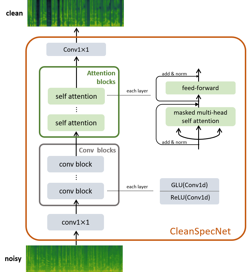
Architecture. CleanSpecNet is composed of a stack of convolutional layers followed by a stack of self-attention blocks [31]. Each convolutional layer is composed of an 1-D convolution (Conv1d) that keeps channels, rectified linear unit (ReLU), another Conv1d that doubles channels, and a gated linear unit (GLU). Each Conv1d has kernel size and stride . Each self-attention block contains: i) a multi-head self-attention layer with 8 heads, 512 model dimensions, and a causal attention mask, and ii) a position-wise fully-connected layer. The architecture is shown in Fig. 1.
Loss Function. Let be the magnitude of the linear spectrogram of waveform , where is the set of hyperparameters used to compute STFT: the hop size, the window length, and the FFT bin. Let be the corresponding hyperparameters for CleanSpecNet. We use to transform noisy waveform to noisy spectrogram , and clean waveform to clean spectrogram . Then, the loss function is
| (1) |
where is the length of spectrogram.
2.4 CleanUNet 2

Architecture. We use the CleanUNet proposed in [27] as the waveform-based module. It is composed of encoder layers, self-attention blocks as bottleneck, and decoder layers that connect with encoder layers by skip connections. After we compute denoised spectrogram with CleanSpecNet, we up-sample it 256 times through 2 transposed 2-d convolutions (stride in time , 2-D filter sizes ), each followed by a leaky ReLU with negative slope . Then, we combine noisy waveform and up-sampled spectrogram through a conditioning method and feed them into CleanUNet. The architecture is demonstrated in Fig. 2. We use element-wise addition as our main conditioning method. Other methods such as concatenation on channels, or FiLM [36] lead to similar results (see Section 3.2).
Loss Function. Similar to CleanUNet [27], we use the addition of waveform loss and multi-resolution STFT losses [37] as the loss function to train CleanUNet 2. In detail, the full-band multi-resolution STFT loss is
| (2) |
where are STFT hyperparameters for different resolutions. The high-band loss replaces with , which contains the high frequency half of (for example, 4-8kHz range for 16kHz audio). The high-band loss can reduce low frequency noises during silence and thus improve actual sound quality [27].
| Model | Domain | PESQ | PESQ | STOI | pred. | pred. | pred. | MOS | MOS | MOS |
| (WB) | (NB) | (%) | CSIG | CBAK | COVRL | SIG | BAK | OVRL | ||
| Noisy dataset | - | 1.585 | 2.164 | 91.6 | 3.190 | 2.533 | 2.353 | - | - | - |
| DTLN [18] | Time-Freq | - | 3.04 | 94.8 | - | - | - | - | - | - |
| PoCoNet [19] | Time-Freq | 2.745 | - | - | 4.080 | 3.040 | 3.422 | - | - | - |
| FullSubNet [17] | Time-Freq | 2.897 | 3.374 | 96.4 | 4.278 | 3.644 | 3.607 | 3.97 | 3.72 | 3.75 |
| Conv-TasNet [38] | Waveform | 2.73 | - | - | - | - | - | - | - | - |
| FAIR-denoiser [26] | Waveform | 2.659 | 3.229 | 96.6 | 4.145 | 3.627 | 3.419 | 3.68 | 4.10 | 3.72 |
| CleanUNet (+full) [27] | Waveform | 3.146 | 3.551 | 97.7 | 4.619 | 3.892 | 3.932 | 4.03 | 3.89 | 3.78 |
| CleanUNet (+high) [27] | Waveform | 3.011 | 3.460 | 97.3 | 4.513 | 3.812 | 3.800 | 3.94 | 4.08 | 3.87 |
| CleanUNet 2 (+full) | Hybrid | 3.262 | 3.658 | 97.7 | 4.661 | 3.976 | 4.030 | 4.11 | 3.92 | 3.86 |
| CleanUNet 2 (+high) | Hybrid | 3.146 | 3.592 | 97.6 | 4.553 | 3.934 | 3.904 | 4.02 | 4.10 | 4.01 |
| Spectrogram Hyperparameters | Model | PESQ | PESQ | STOI | pred. | pred. | pred. | ||
| Window Length | Hop Size | FFT Bin | (WB) | (NB) | (%) | CSIG | CBAK | COVRL | |
| 1024 | 256 | 1024 | CleanSpecNet | 2.874 | 3.261 | 96.2 | 4.388 | 3.455 | 3.649 |
| CleanUNet 2 | 3.262 | 3.658 | 97.7 | 4.661 | 3.976 | 4.030 | |||
| 512 | 256 | 512 | CleanSpecNet | 3.048 | 3.491 | 96.2 | 4.500 | 3.565 | 3.805 |
| CleanUNet 2 | 3.257 | 3.651 | 97.7 | 4.659 | 3.969 | 4.025 | |||
| 320 | 80 | 320 | CleanSpecNet | 3.071 | 3.565 | 97.0 | 4.526 | 3.679 | 3.847 |
| CleanUNet 2 | 3.166 | 3.571 | 97.6 | 4.606 | 3.925 | 3.944 | |||
| Spectrogram Hyperparameters | Model | PESQ | PESQ | STOI | pred. | pred. | pred. | ||
| Window Length | Hop Size | FFT Bin | (WB) | (NB) | (%) | CSIG | CBAK | COVRL | |
| 1024 | 256 | 1024 | CleanSpecNet | 2.925 | 3.289 | 96.3 | 4.437 | 3.483 | 3.700 |
| CleanUNet 2 (+full) | 3.349 | 3.698 | 97.8 | 4.711 | 4.036 | 4.110 | |||
| CleanUNet 2 (+high) | 3.319 | 3.679 | 97.8 | 4.695 | 3.999 | 4.082 | |||
| 320 | 80 | 320 | CleanSpecNet | 3.149 | 3.623 | 97.4 | 4.583 | 3.731 | 3.922 |
| CleanUNet 2 (+full) | 3.302 | 3.681 | 97.9 | 4.689 | 3.995 | 4.065 | |||
| CleanUNet 2 (+high) | 3.219 | 3.607 | 97.7 | 4.642 | 3.926 | 3.988 | |||
3 Experiment
In this section, we evaluate CleanUNet 2 on the Deep Noise Suppression (DNS) dataset [8]. We compare it with other state-of-the-art (SOTA) spectrogram and waveform-based models with several objective and subjective evaluation metrics. The main results are summarized in Tables 1 and 2.
3.1 Setup
Data preparation. The DNS 2020 dataset [8] contains 441 hours of clean speech (2150 speakers reading books) and 70K noise clips, all under 16kHz sampling rate. The training set is composed of 500 hours clean-noisy speech pairs with 31 SNR levels ranging from to dB [8]. For each waveform pair , we first compute spectrogram pair . Then, we take aligned 10-second random clips from waveform and spectrogram.
Hyperparameters. The hyperparameters for CleanUNet are the following: it has 8 encoder/decoder layers, each with hidden dimension , stride , and kernel size . It has 5 self-attention blocks, each with 8 heads, model dimension , no dropout and no positional encoding. The hyperparemeters for CleanSpecNet are the following: it has 5 convolutional layers, each with hidden dimension , stride , and kernel size . It has 5 self-attention blocks same as CleanUNet.
Optimization. The optimizer is an Adam optimizer with and . The learning rate scheduler is the linear warmup (ratio ) with cosine annealing, where the maximum learning rate is . The CleanSpecNet is trained to minimize Eq. (1), with a batchsize of 64 and 1M iterations. We use multi-resolution hop sizes in , window lengths in , and FFT bins in . All models are trained on 8 NVIDIA V100 GPUs.
We study different spectrogram hyperparameters in Section 3.2. The CleanUNet 2 is trained to minimize the full or high-band losses described in Section 2.4, with a batchsize of 32 and 500K iterations.
Evaluation. We use objective and subjective metrics to evaluate quality of denoised speech. Objective metrics include: Perceptual Evaluation of Speech Quality (PESQ, where WB means wide-band and NB means narrow-band) [39], Short-Time Objective Intelligibility (STOI) [40], and Mean Opinion Score (MOS) prediction of the a) distortion of speech signal (SIG), b) intrusiveness of background noise (BAK), and c) overall quality (OVRL) [41]. We also use the subjective MOS evaluations recommended in ITU-T P.835 [42]. We randomly select 100 samples from the test set. Each utterance is scored by 15 workers in three dimensions: SIG, BAK, and OVRL.
3.2 Main Results
CleanUNet 2: We compare CleanUNet 2 with several SOTA models. Similar to [27], we study both full and high-band STFT losses described in Section 2.4. Table 1 demonstrates objective and subjective evaluations on the no-reverb testset. CleanUNet 2 outperforms all baselines in objective evaluations. On average, there is a significant boost () in PESQ. In terms of subjective evaluation, CleanUNet 2 also outperforms CleanUNet with comparable configurations (e.g., loss combinations).
To test the statistical significance of improvement, we conduct the Wilcoxon signed-rank test between CleanUNet 2 and baseline models with respect to PESQ, STOI, and MOS OVRL. The -values are shown in Table 4. Results indicate CleanUNet 2 performs consistently better than baseline models in these objective and subjective metrics.
| Metric | Baseline Model | -value |
| PESQ (WB) | CleanUNet (+high) | |
| FullSubNet | ||
| FAIR-denoiser | ||
| STOI | CleanUNet (+high) | |
| FullSubNet | ||
| FAIR-denoiser | ||
| MOS OVRL | CleanUNet (+high) | |
| FullSubNet | ||
| FAIR-denoiser |
CleanSpecNet: We study the effect of spectrogram hyperparameters in CleanSpecNet and the resulting CleanUNet 2. To obtain denoised speech with the denoised spectrogram generated by CleanSpecNet, we extract phase information from noisy speech, and apply inverse STFT to the denoised spectrogram and the phase.
Results on objective evaluations are shown in Table 2. First, we note that CleanSpecNet with a window length of 320 is a highly competitive denoiser by itself. Second, CleanUNet 2 always improves over CleanSpecNet. Third, we find for CleanSpecNet, smaller window lengths and hop sizes lead to better quality (see underlined scores), while it is the opposite for CleanUNet 2. This means a better spectrogram model does not always lead to a better hybrid model. Interestingly, the best performance of CleanUNet 2 (PESQ: 3.262) is achieved by combining the waveform model with a spectrogram-based model (CleanSpecNet) using typical neural vocoder STFT parameters (i.e., Window Length 1024 and Hop Size 256). This empirical evidence highlights our motivation of using two-stage speech synthesis pipeline to improve the speech denosing results.
Conditioning Methods: We study different conditioning methods in Table 5. We use the set of hyperparameters whose window length is 1024, and optimize with the high-band loss. These methods lead to very similar results. Since the element-wise addition is the simplest and leads to the smallest model footprint, we use this conditioning method in CleanUNet 2.
| Conditioning | PESQ (WB) | STOI (%) | pred. COVRL |
| Addition | 3.146 | 97.6 | 3.904 |
| Concatenation | 3.146 | 97.6 | 3.909 |
| FiLM [36] | 3.136 | 97.6 | 3.893 |
3.3 Inference Speed and Latency
We compare inference speed among FAIR-denoiser, CleanUNet, CleanSpecNet and the full CleanUNet 2. We use real time factor (RTF) to measure inference speed. RTF is defined as the time to generate some speech divided by its total time. We use batchsize , length seconds, and sampling rate Hz. Results are in Table 6.
Note that, CleanUNet 2 has 16 ms latency for 16kHz audio, which comes from the temporal downsampling (i.e., 256) from the original time-domain waveform to the bottleneck hidden representation (between encoder and decoder) its waveform submodule. In a streaming system, one may cache previous hidden representation, and wait until the next 256 waveform samples (correspond to 16 ms) to compute the most current hidden state.
| Model | RTF |
| FAIR-denoiser | |
| CleanUNet | |
| CleanSpecNet | |
| CleanUNet 2 |
3.4 Non-causal Speech Denoising Models
We evaluate denoising quality of non-causal versions of our models. These models are also useful, as they can be used for offline denoising in applications where real-time denoising is not necessary. The non-causal models are obtained by removing the causal attention masks. Results are shown in Table 3.
4 Related Work
We notice that a few hybrid models are proposed for speech denoising in previous study. [43] proposes a joint network composed of a spectrogram-based network followed by a waveform decoder. Different from our CleanUNet 2, their network only takes the noisy spectrogram as input, which may lose information from the noisy waveform. In addition, their network is not causal. [44] proposes a neural cascade architecture with triple-domain losses. [45] decouples the joint optimization of spectrogram magnitude and phase into two sub-tasks; only magnitude is predicted in the first stage. After that, both the magnitude and phase components are refined in the second stage. [46] suppress the noise in the spectrogram magnitude at one path, and try to compensate for the lost spectral detail in the complex domain at another path.
5 Conclusion
We introduce CleanUNet 2, a hybrid speech denoising model. It first applies a spectrogram-based model to denoise spectrogram, and then uses it to condition a waveform-based model (CleanUNet), which outputs denoised waveform. For both sub-modules we use self-attention to refine the representation. We test CleanUNet 2 on DNS; it achieves the state-of-the-art speech denoising quality in both objective and subjective evaluations.
References
- [1] P. C. Loizou, Speech enhancement: theory and practice. CRC press, 2007.
- [2] S. Boll, “Suppression of acoustic noise in speech using spectral subtraction,” IEEE Transactions on acoustics, speech, and signal processing, 1979.
- [3] J. S. Lim and A. V. Oppenheim, “Enhancement and bandwidth compression of noisy speech,” Proceedings of the IEEE, vol. 67, no. 12, pp. 1586–1604, 1979.
- [4] S. Tamura and A. Waibel, “Noise reduction using connectionist models,” in ICASSP. IEEE, 1988.
- [5] S. Parveen and P. Green, “Speech enhancement with missing data techniques using recurrent neural networks,” in ICASSP, 2004.
- [6] X. Lu et al., “Speech enhancement based on deep denoising autoencoder.” in Interspeech, 2013.
- [7] Y. Xu et al., “A regression approach to speech enhancement based on deep neural networks,” IEEE/ACM Transactions on Audio, Speech, and Language Processing, 2014.
- [8] C. K. Reddy et al., “The interspeech 2020 deep noise suppression challenge: Datasets, subjective testing framework, and challenge results,” arXiv, 2020.
- [9] M. Soni et al., “Time-frequency masking-based speech enhancement using generative adversarial network,” in ICASSP, 2018.
- [10] S.-W. Fu et al., “MetricGAN: Generative adversarial networks based black-box metric scores optimization for speech enhancement,” in ICML, 2019.
- [11] ——, “MetricGAN+: An improved version of metricgan for speech enhancement,” arXiv, 2021.
- [12] Y. Wang and D. Wang, “A deep neural network for time-domain signal reconstruction,” in ICASSP, 2015.
- [13] F. Weninger et al., “Speech enhancement with lstm recurrent neural networks and its application to noise-robust asr,” in International conference on latent variable analysis and signal separation, 2015.
- [14] A. Nicolson and K. K. Paliwal, “Deep learning for minimum mean-square error approaches to speech enhancement,” Speech Communication, 2019.
- [15] F. G. Germain et al., “Speech denoising with deep feature losses,” arXiv, 2018.
- [16] Y. Xu et al., “Multi-objective learning and mask-based post-processing for deep neural network based speech enhancement,” arXiv, 2017.
- [17] X. Hao et al., “Fullsubnet: A full-band and sub-band fusion model for real-time single-channel speech enhancement,” in ICASSP, 2021.
- [18] N. Westhausen and B. Meyer, “Dual-signal transformation lstm network for real-time noise suppression,” arXiv, 2020.
- [19] U. Isik et al., “Poconet: Better speech enhancement with frequency-positional embeddings, semi-supervised conversational data, and biased loss,” arXiv, 2020.
- [20] D. S. Williamson et al., “Complex ratio masking for monaural speech separation,” IEEE/ACM transactions on audio, speech, and language processing, 2015.
- [21] S. Pascual et al., “Segan: Speech enhancement generative adversarial network,” arXiv, 2017.
- [22] S.-W. Fu, Y. Tsao, X. Lu, and H. Kawai, “Raw waveform-based speech enhancement by fully convolutional networks,” in Asia-Pacific Signal and Information Processing Association Annual Summit and Conference. IEEE, 2017.
- [23] D. Rethage et al., “A wavenet for speech denoising,” in ICASSP, 2018.
- [24] A. Pandey and D. Wang, “TCNN: Temporal convolutional neural network for real-time speech enhancement in the time domain,” in ICASSP, 2019.
- [25] X. Hao et al., “UNetGAN: A robust speech enhancement approach in time domain for extremely low signal-to-noise ratio condition,” in Interspeech, 2019.
- [26] A. Defossez et al., “Real time speech enhancement in the waveform domain,” in Interspeech, 2020.
- [27] Z. Kong, W. Ping, A. Dantrey, and B. Catanzaro, “Speech denoising in the waveform domain with self-attention,” in ICASSP 2022-2022 IEEE International Conference on Acoustics, Speech and Signal Processing (ICASSP). IEEE, 2022, pp. 7867–7871.
- [28] A. v. d. Oord et al., “WaveNet: A generative model for raw audio,” arXiv, 2016.
- [29] O. Ronneberger et al., “U-Net: Convolutional networks for biomedical image segmentation,” in MICCAI, 2015.
- [30] D. Stoller et al., “Wave-U-Net: A multi-scale neural network for end-to-end audio source separation,” arXiv, 2018.
- [31] A. Vaswani et al., “Attention is all you need,” in NIPS, 2017.
- [32] W. Ping, K. Peng, A. Gibiansky, S. O. Arik, A. Kannan, S. Narang, J. Raiman, and J. Miller, “Deep voice 3: Scaling text-to-speech with convolutional sequence learning,” in ICLR, 2018.
- [33] J. Shen, R. Pang, R. J. Weiss, M. Schuster, N. Jaitly, Z. Yang, Z. Chen, Y. Zhang, Y. Wang, R. Skerrv-Ryan et al., “Natural tts synthesis by conditioning wavenet on mel spectrogram predictions,” in ICASSP, 2018.
- [34] W. Ping, K. Peng, and J. Chen, “ClariNet: Parallel wave generation in end-to-end text-to-speech,” in ICLR, 2019.
- [35] W. Ping, K. Peng, K. Zhao, and Z. Song, “WaveFlow: A compact flow-based model for raw audio,” in ICML, 2020.
- [36] E. Perez et al., “Film: Visual reasoning with a general conditioning layer,” in AAAI, 2018.
- [37] R. Yamamoto et al., “Parallel WaveGAN: A fast waveform generation model based on generative adversarial networks with multi-resolution spectrogram,” in ICASSP, 2020.
- [38] Y. Luo and N. Mesgarani, “Conv-tasnet: Surpassing ideal time–frequency magnitude masking for speech separation,” IEEE/ACM transactions on audio, speech, and language processing, 2019.
- [39] I.-T. Recommendation, “Perceptual evaluation of speech quality (pesq): An objective method for end-to-end speech quality assessment of narrow-band telephone networks and speech codecs,” Rec. ITU-T P. 862, 2001.
- [40] C. H. Taal et al., “An algorithm for intelligibility prediction of time–frequency weighted noisy speech,” IEEE Transactions on Audio, Speech, and Language Processing, 2011.
- [41] Y. Hu and P. C. Loizou, “Evaluation of objective quality measures for speech enhancement,” IEEE Transactions on Audio, Speech, and Language Processing, 2008.
- [42] ITUT, “Subjective test methodology for evaluating speech communication systems that include noise suppression algorithm,” ITU-T recommendation, 2003.
- [43] C. Tang, C. Luo, Z. Zhao, W. Xie, and W. Zeng, “Joint time-frequency and time domain learning for speech enhancement,” in IJCAI, 2021.
- [44] H. Wang and D. Wang, “Neural cascade architecture with triple-domain loss for speech enhancement,” IEEE/ACM Transactions on Audio, Speech, and Language Processing, vol. 30, pp. 734–743, 2021.
- [45] A. Li, W. Liu, C. Zheng, C. Fan, and X. Li, “Two heads are better than one: A two-stage complex spectral mapping approach for monaural speech enhancement,” IEEE/ACM Transactions on Audio, Speech, and Language Processing, 2021.
- [46] A. Li, C. Zheng, L. Zhang, and X. Li, “Glance and gaze: A collaborative learning framework for single-channel speech enhancement,” Applied Acoustics, 2022.