Share Your Representation Only: Guaranteed Improvement of the Privacy-Utility Tradeoff in Federated Learning
Abstract
Repeated parameter sharing in federated learning causes significant information leakage about private data, thus defeating its main purpose: data privacy. Mitigating the risk of this information leakage, using state of the art differentially private algorithms, also does not come for free. Randomized mechanisms can prevent convergence of models on learning even the useful representation functions, especially if there is more disagreement between local models on the classification functions (due to data heterogeneity). In this paper, we consider a representation federated learning objective that encourages various parties to collaboratively refine the consensus part of the model, with differential privacy guarantees, while separately allowing sufficient freedom for local personalization (without releasing it). We prove that in the linear representation setting, while the objective is non-convex, our proposed new algorithm CENTAUR converges to a ball centered around the global optimal solution at a linear rate, and the radius of the ball is proportional to the reciprocal of the privacy budget. With this novel utility analysis, we improve the SOTA utility-privacy trade-off for this problem by a factor of , where is the input dimension. We empirically evaluate our method with the image classification task on CIFAR10, CIFAR100, and EMNIST, and observe a significant performance improvement over the prior work under the same small privacy budget. The code can be found in this link.
1 Introduction
In federated learning (FL), multiple parties cooperate to learn a model under the orchestration of a central server while keeping the data local. However, this paradigm alone is insufficient to provide rigorous privacy guarantees, even when local parties only share partial information (e.g. gradients) about their data. An adversary (e.g. one of the parties) can infer whether a particular record is in the training data set of other parties (Nasr et al. 2019), or even precisely reconstruct their training data (Zhu et al. 2019). To formally mitigate these privacy risks, we need to guarantee that any information shared between the parties during the training phase has bounded information leakage about the local data. This can be achieved using FL under differential privacy (DP) guarantees.
FL and DP are relatively well-studied separately. However, their challenges multiply when conducting FL under a DP constraint, in real-world settings where the data distributions can vary substantially across the clients (Li et al. 2020b; Acar et al. 2020; Shen et al. 2022). A direct consequence of such data heterogeneity is that the optimal local models might vary significantly across clients and differ drastically from the global solution. This results in large local gradients (Jiang et al. 2019). However, these large signals leak information about the local training data, and cannot be communicated as such when we need to guarantee DP. We require clipping gradient values (usually by a small threshold (De et al. 2022)) before sending them to the server, to bound the sensitivity of the gradient function with respect to changes in training data Abadi et al. 2016. As the local per-sample gradients (due to data heterogeneity) tend to be large even at the global optimum, clipping per-example gradient by a small threshold and then randomizing it, will result in a high error in the overall gradient computation, and thus degrading the accuracy of the model learned via FL.
Contributions. In this work, we identify an important bottleneck for achieving high utility in FL under a tight privacy budget: There exists a magnified conflict between learning the representation function and classification head, when we clip gradients to bound their sensitivity (which is required for achieving DP). This conflict causes slow convergence of the representation function and disproportional scaling of the local gradients, and consequently leads to the inevitable utility drop in DP FL. To address this issue, we observe that in many FL classification scenarios, participants have minimal disagreement on data representations (Bengio et al. 2013; Chen et al. 2020; Collins et al. 2021), but possibly have very different classifier heads (e.g., the last layer of the neural network). Therefore, instead of solving the standard classification problem, we borrow ideas from the literature of model personalization and view the neural network model as a composition of a representation extractor and a small classifier head, and optimize these two components in different manners. In the proposed scheme, CENTAUR, we train a single differentially private global representation extractor while allowing each participant to have a different personalized classifier head. Such a decomposition has been considered in previous arts like (Collins et al. 2021) and (Singhal et al. 2021), but only in a non-DP setting, and also in (Jain et al. 2021), but only for a linear embedding case.
Due to low heterogeneity in data representation (compared to the whole model), the DP learned representation in our new scheme outperforms prior schemes that perform DP optimization over the entire model.
In the setting where both the representation function and the classifier heads are linear w.r.t. their parameters, we prove a novel utility-privacy trade-off for an instance of CENTAUR, yielding a significant improvement over previous art, where is the input dimension (Corollary 5.1). A major algorithmic novelty of our proposed approach is a cross-validation scheme for boosting the success probability of the classic noisy power method for privacy-preserving spectral analysis.
We present strong empirical evidence for the superior performance of CENTAUR over the prior work, under the small DP budget of () in a variety of data-heterogeneity settings on benchmark datasets CIFAR10, CIFAR100, and EMNIST. Our method outperforms the prior work in all settings. Moreover, we showcase that CENTAUR uniformly enjoys a better utility-privacy trade-off over its competitors on the CIFAR10 dataset across different privacy budget (Figure 1). Importantly, CENTAUR outperforms the local stand-alone training even with, , thus justifying the benefit of collaborative learning compared to stand-alone training for a larger range of privacy budget.
1.1 Related Work
Federated learning with differential privacy has been extensively studied since its emergence (Shokri & Shmatikov 2015; McMahan et al. 2017a). Without any trusted central party, the local differential privacy model requires each client to randomize its messages before sending them to other (malicious) parties. Consequently, the trade-off between local DP and accuracy is significantly worse than that for centralized setting and requires huge amount of data for learning even simple statistics (Duchi et al. 2014; Erlingsson et al. 2014; Ding et al. 2017). By using secure aggregation protocol,
recent works (McMahan et al. 2017b; Agarwal et al. 2018; Levy et al. 2021; Kairouz et al. 2021) study user-level DP under Billboard model to enable better utility. We also focus on such user-level DP setting under Billboard model.
Model personalization approaches (Smith et al. 2017; Fallah et al. 2020; Li et al. 2020b; Arivazhagan et al. 2019; Collins et al. 2021; Pillutla et al. 2022) enable each client to learn a different (while related) model, thus alleviating the model drifting issue due to data heterogeneity. Recent works further investigate whether model personalization approaches enable improved privacy accuracy trade-off for federated learning. Hu et al. 2021 propose a private federated multi-task learning algorithm by adding task-specific regularization to each client’s optimization objective. However, the regularization
has limited ability to deal with data heterogeneity. Bietti et al. 2022 propose the PPSGD algorithm that enables training additive personalized models with user-level DP. However, their generalization guarantees crucially rely on the convexity of loss functions. On the contrary, we study the convergence of CENTAUR algorithm under more general non-convex objectives.
The closest prior work to our approach in the literature is Jain et al. 2021, who also propose differentially privately learning shared low-dimensional linear representation with individualized classification head. However, their algorithm relies on solving the least square problem exactly at server side, by performing SVD on perturbed noisy representation matrix. Hence, the generalization guarantee of their algorithm intrinsically has an expensive dependency on the data dimension . By contrast, we perform noisy gradient descent at server side and improve upon this error dependency by a factor of . Their algorithm is also limited to the linear representation learning problem, unlike our CENTAUR algorithm which enables training multiple layers of shared representations. Upon submitting this paper, we became aware of a recent concurrent work Xu et al. 2023 that uses a very similar algorithm to learn image embedding (representation) with user-level differential privacy in the extreme multi-class setting (i.e., when the classifier is extremely large).
Our work builds on the FedRep algorithm (Collins et al. 2021), which also relies on learning shared representations between clients but does not consider privacy. In contrast, our work provides a novel private and federated representation learning framework. Moreover, a major different ingredient of our algorithm is the initialization procedure, which requires performing differentially private SVD to the data matrix. We use the noisy power method (Hardt & Price 2014) as a crucial tool to enable a constant probability for utility guarantee. We then perform cross-validation to further boost success probability to arbitrarily large (inspired by Liang et al. 2014).
2 Notations and Background on Privacy
Notations. We denote the clipping operation by , and denote the Gaussian mechanism as where .
Define Rényi Differential Privacy (RDP) on a dataset space equipped with a distance as follows.
Definition 2.1 (RDP).
For measures over the same space with , their Rényi divergence . A randomized algorithm satisfies -RDP, if with , we have .
User-level-RDP.
Let be the space of all of tuples of local datasets , where each local dataset consists of data points, i.e. .
The distance is the Hamming distance in the dataset level, i.e. . We refer to the privacy guarantee recovered by this choice of dataset space as user-level-RDP.
In Appendix A.3, we further describe the Gaussian Mechanism and the composition of RDP, the standard notion of Differential Privacy (DP), and the conversion Lemma from RDP to DP.
Threat Models. We aim to protect the privacy of each user against potential adversarial other clients, i.e., any eavesdropper will not be able to tell whether one users has participated in the collaborative learning procedure, given the information released during training phase. We establish user-level RDP guarantees under the billboard model, which is a communication protocol that is particularly compatible with algorithms in the federated setting and has been adopted in many previous works (Jain et al. 2021; Hu et al. 2021; Bietti et al. 2022). In this model, a trusted server (either a trusted party or one that uses cryptographic techniques like multiparty computation) aggregates information subject to a DP constraint, which is then shared as public messages with all the users. Then, each user computes its own personalized model based on the public messages and its own private data (Hsu et al. 2014). Our RDP guarantees only hold for releasing the shared representations in Algorithm 1, and the guarantees are equivalent to joint-(R)DP guarantees Kearns et al. 2014 if all the personalized models of individual users were additionally released as outputs of Algorithm 2.
3 Problem Formulation
Consider a Federated Learning (FL) setting where there are agents interacting with a central server and the th agent holds local data points . Here denotes a pair of an input vector and the corresponding label. Suppose that each local dataset is sampled from an underlying joint distribution of the input and response pair. We consider the data-heterogenous setting where potentially for . We further consider a hypothesis model which maps an input to the predicted label . Here is the trainable parameter of the model . Let be a loss function that penalizes the error of the prediction given the true label . The local objective on client is defined as
| (1) |
The standard FL formulation seeks a global consensus solution, whose objective is defined as
| (2) |
While this formulation is reasonable when the local data distributions are similar, the obtained global solution may be far from the local optima under diverse local data distributions, a phenomenon known as statistical heterogeneity in the FL literature (Li et al. 2020a; Wang et al. 2019; Malinovskiy et al. 2020; Mitra et al. 2021; Charles & Konečnỳ 2021; Acar et al. 2020; Karimireddy et al. 2020). Such a (potentially significant) mismatch between local and global optimal solutions limits the incentive for collaboration, and cause extra difficulties when DP constraints are imposed (Remark 3.1). These considerations motivate us to search for personalized solutions that can be learned in a federated fashion, with less utility loss due to the DP constraint.
Federated representation learning with differential privacy.
It is now well-documented that in some common and real-world FL tasks, such as image classification and word prediction, clients have minimal disagreement on data representations (Chen et al. 2020; Collins et al. 2021). Based on this observation, a more reasonable alternative to the FL objective in equation 2 should focus on learning the data representation, which is the information that is agreed on among most parties, while also allowing each client to personalize its learning on information that the other clients disagree on. To formalize this, suppose that the variable can be partitioned into a pair with and the parameterized model admits the composition where is the representation extractor that maps -dimensional data points to a lower dimensional space of size and is a classifier head that maps from the lower dimensional subspace to the space of labels. An important example is bottom and top layers of the neural network model. We use and to denote the parameters that determine and , respectively. With the above notation, we consider the following federated representation learning (FRL) problem
| (3) |
where we maintain a single global representation extraction function subject to the constraint while allowing each client to use its personalized classification head locally. The constraint is included so that equation 3 also covers the linear case studied in section 5.
The choice of the FRL formulation in equation 3 entails considerations from both DP and optimization perspectives: From the DP standpoint, the phenomenon of statistical heterogeneity introduces additional difficulties for federated learning under DP constraint (see Remark 3.1 below). If the clients collaborate to train only a shared representation function, then the aforementioned disadvantages can be alleviated; From the optimization standpoint, we typically have , i.e. the dimension of the extracted features is much smaller than that of the original input. Hence, for a fixed representation function , the client specific heads are in general easy to optimize locally as the number of parameters, , is typically small.
Remark 3.1 (Statistical heterogeneity makes DP guarantee harder to establish.).
To establish DP guarantees for gradient based methods, e.g. DP-SGD, a common choice is the Gaussian mechanism, which is comprised of the gradient clipping step and the noise injection step. It is empirically observed that to achieve a better privacy-utility trade-off, a small clipping threshold is preferred, since it limits the large variance due to the injected noise (De et al. 2022). Moreover, the effect of the bias (due to clipping) subsides as the per-sample gradient norm diminishes during the centralized training, a phenomenon known as benign overfitting in deep learning (Bartlett et al. 2020; Li et al. 2021; Bartlett et al. 2021).
However, due to the phenomenon of distribution shift, the local (per-sample) gradients in the standard FL setting (described in equation 2) remain large even at the global optimal solution, and hence setting a small (per-sample) gradient clipping threshold will result in a large and non-diminishing bias in the overall gradient computation.
In contrast, for tasks where the representation extracting functions are approximately homogeneous, the local and global optimal of the FRL formulation 3 are close and hence the gradients w.r.t. the representation function vanishes at the optimal, which is amiable to small clipping threshold.
4 Differential Private Federated Representation Learning
In this section we present the proposed CENTAUR method to solve the FRL problem in equation 3.
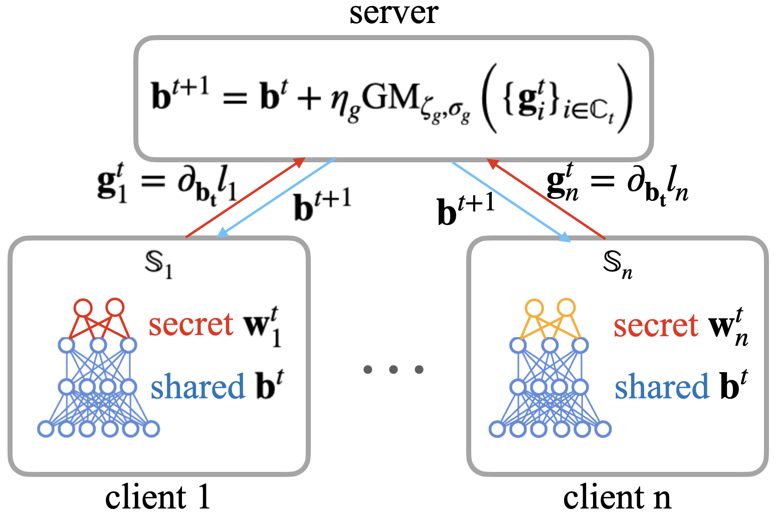
Server procedure (Algorithm 1) takes the following quantities as inputs: denotes the initializer for the parameter of the global representation function, obtained from a procedure Initialization; denotes the portion of the clients that will participate in training per global communication round; denotes the total number of global communication rounds; denotes the global update step size; stand for the noise multiplier and the clipping threshold of the Gaussian mechanism (that ensures user-level RDP). Note that in this section, we consider random Initialization over unconstrained space , and the procedure Under these configurations, Server follows the standard FL protocol: After broadcasting the current global representation function to the activate clients, it aggregates the information returned from the Client procedure to update the global representation function.
Client procedure (Algorithm 2) takes the following quantities as inputs: denotes the parameter of the global representation function received from the server; denotes the number of local data points used as mini-batch to update the local representation function; denotes the number of local update iterations; denotes the local update step size. Client can be divided into three phases: 1. After receiving the current global parameter of the representation function from the server, the client update the local classifier head to the minimizer of the local objective . This is possible since the local objective usually admits very simple structure, e.g. it is convex w.r.t. , once the representation function is fixed. In practice, we would run multiple SGD epochs on to approximately minimize with fixed. This is computationally cheap since the dimension of is much smaller compared to the whole variable . 2. Once the local classifier head is updated to , the client optimizes its local representation function with multiple SGD steps, starting from the current global consensus . 3. Finally, each client calculate its local update direction for representation via the difference between its latest local representation function and the previous global consensus, .
Remark 4.1 (Privacy guarantee).
By the composition theorem for subsampled Gaussian Mechanism Mironov et al. 2019, we prove that Algorithm 1 and Algorithm 2 satisfies user-level -Rényi differential privacy for , where . In the special case of full gradient descent with , we have that .
5 Guaranteed Improvement of the Utility-Privacy Trade-off
In the previous section, we present CENTAUR for the general FRL problems (3). Due to the lack of structure information, for a general non-convex optimization problem we cannot expect any utility guarantee beyond the convergence to a stationary point. In this section, we consider a specific instance of the FRL problems where both the representation function and the local classifiers are linear w.r.t. their parameters and . This model has been commonly used in the analysis of representation learning (Collins et al. 2021; Collins et al. 2022), meta learning (Tripuraneni et al. 2021; Du et al. 2020; Thekumparampil et al. 2021; Sun et al. 2021), model personalization (Jain et al. 2021), multi-task learning (Maurer et al. 2016). For this (still nonconvex) instance, we prove that CENTAUR converges to a ball centered around the global minimizer in a linear rate where the size of the ball depends on the required RDP parameters (). Let be the utility and let be the DP-parameter (CENTAUR is an -DP mechanism). We obtain the improved privacy-utility tradeoff , which is better than the current SOTA result, , by (Jain et al. 2021). In the following, we will first review objective (3) in the linear representation setting, and analyse CENTAUR to show the improved utility-privacy tradeoff.
Federated Linear Representation Learning (LRL)
Recall the problem formulation in Section 3.
For simplicity, we assume for all for some constant .
Consider the LRL setting, where given the input the response satisfies
. 11
1
A similar problem is considered in (Jain et al. 2021), but the measurement suffers from an extra white noise with variance . In our paper, we consider the noiseless case and hence when comparing with (Jain et al. 2021), we treat the in their results for a fair comparison.
Here is a column orthonormal global representation matrix and is an agent-specific optimal local linear classifiers.
In terms of the notations, corresponds to the parameter in the general formulation (3), but is capitalized since it is now regarded as a matrix. The feasible domain is the set of column orthonormal matrices .
Given a local dataset (could be or its subset), define
| (4) |
Our goal is to recover the ground truth representation matrix using the collection of the local datasets via solving the following linear instance of the FRL problem equation 3
| (L-FRL) |
in a federated and DP manner. Here, equation L-FRL is an instance of the general FRL problem (3) with and set to linear functions and set to the least square loss. Note that, despite the (relatively) simple structure of equation L-FRL, it is still non-convex w.r.t. the variable .
Methodology for the LRL case.
To establish our novel privacy and utility guarantees, we need to specify Initialization and Aggregation in the procedures Server and we also need to slightly modify the Client procedure, which are elaborated as follows.
1. To obtain the novel guarantee of converging to the global minimizer for the LRL case, the initializer needs to be within a constant distance to the global optimal which requires a more sophisticated procedure than the simple random initialization.
We show that this requirement can be ensured by running a modified instance of the private power method (PPM) by (Hardt & Price 2014), but the utility guarantee only holds with a constant probability (Lemma F.1).
A key contribution of our work is to propose a novel cross-validation scheme to boost the success probability of the PPM with a small extra cost.
Our scheme only takes as input the outputs of independent PPM trials, and hence can be treated as post-processing, which is free of privacy risk (Lemma F.3).
The proposed Initialization procedure is presented in Algorithm 3.
The analyses are deferred to Appendix F.
2. As discussed earlier, the feasible domain is the set of column orthonormal matrices. In order to ensure the feasibility of , we set ,
where denotes the QR decomposition and only returns the matrix.
3.
We make a small modification in line 2 where two subsets and of the local dataset are sampled without replacement from and are used to replace in Phases 1 and 2. This change is required to establish our novel utility result, which ensures that clipping threshold of the Gaussian mechanism (line 7) in the Server procedure is never reached with a high probability (Lemma C.1).
5.1 Analysis of CENTAUR in the LRL setting
Use to denote the th largest singular value of a matrix . Let be the collection of the local optimal classifier heads with . We use as a shorthand for and use to denote the condition number of the problem. We choose the scaling such that remains meaningful as . We make the following assumptions.
Assumption 5.1.
is zero mean, -covariance, -subgaussian (defined in Appendix A.1).
Assumption 5.2.
There exists a constant such that .
Assumption 5.3.
The number of local data points is sufficiently large: . Here hides the dependence on , , and the log factors.
These assumptions are standard in literature (Collins et al. 2021; Jain et al. 2021). An elaborated discussion is provided in Appendix K. While Problem (L-FRL) is non-convex, we show that the consensus representation converges to a ball centered around the ground truth solution in a linear rate. The size of the ball is controlled by the noise multiplier , which will be the free parameter that controls the utility-privacy tradeoff.
High level idea. For Problem (L-FRL), we find an initial point close to the ground truth solution via the method of moments.
Given this strong initialization, CENTAUR converges linearly to the vicinity of the ground truth since it can be interpreted as an inexact gradient descent method with a fast decreasing bias term.
One caveat that requires particular attention is the clipping step in the Gaussian mechanism (line 5 in Algorithm 4) will destroy the above interpretation if the threshold parameter is set too small.
To resolve this, we set to be a high probability upper bound of so that the clipping step only takes effect with a negligible probability.
In the utility analysis of the LRL case, we use the principal angle distance to measure the convergence of the column-orthonormal variable towards the ground truth . We also refer to this quantity as the utility of the algorithm. Let be the orthogonal complement of . We define
To simplify the presentation of the result, we make the following assumptions: The dimension of the input is sufficiently large and the number of clients is sufficiently large . The proof of the following theorem can be find in Appendix C.
Theorem 5.1 (Utility Analysis).
Consider the instance of CENTAUR for the LRL setting with its Client and Initialization procedures defined in Algorithms 4 and 3 respectively. Suppose that the matrix returned by Initialization satisfies , and suppose that the mini-batch size parameter satisfies Set the clipping threshold of the Gaussian mechanism , the global step size , the number of global rounds . Assuming that the noise multiplier in the Gaussian mechanism is sufficiently small22 2 The intuition behind this requirement is that our convergence analysis requires the iterates to stay within a ball centered around the ground truth, with a constant radius (measured in terms of the principal angle distance). Adding a large noise will break this argument. Similar requirements are made in Tripuraneni et al. 2021.: . Let , , , , and be universal constants. We have with probability at least , . 33 3 Note that Jain et al. 2021 use the Frobenius norm (instead of the spectral norm) of as the optimality metric. However, since , we can always bound . With this extra factor, Theorem 5.1 quadratically depends on , same as Lemma 4.4 in (Jain et al. 2021), while the dependency on is substantially reduced, from to .
Since the Server procedure remains exactly the same as Algorithm 1 in the LRL case, the main body (anything after Initialization) of the resulting CENTAUR instance has the same privacy guarantee as described in remark 4.1. However, we still need to account for the privacy leakage of the Initialization procedure in Algorithm 3 as it is data-dependent. This will be deferred to Appendix F, where we show that Algorithm 3 is an -RDP mechanism, with defined in Corollary F.1. Combining this fact with the RDP analysis for the main body leads to the following privacy guarantee for CENTAUR in the LRL case (see Appendix A.4).
Theorem 5.2 (Privacy Bound).
Consider the instance of CENTAUR with its Client procedure defined in Algorithm 4 and its Initialization procedure defined in Algorithm 3. Suppose that the Initialization procedure is an -RDP mechanism (proved in Corollary F.1). Let , the noise multiple in the Client procedure, be a free parameter that controls the privacy-utility trade-off. By setting the inputs to Server as , , the instance of CENTAUR under consideration is an -RDP mechanism, where . Moreover, when , we have , in which case CENTAUR is an -RDP mechanism and is also an -DP mechanism with .
Overall Utility-Privacy Trade-off We now combine the utility and privacy analyses of CENTAUR in the LRL setting to obtain the overall utility-privacy trade-off in the following sense: According to Theorem 5.1, to achieve a high utility, i.e. a small , we need to choose a small noise multiplier while Theorem 5.2 states that the smaller is, the larger the privacy cost.
Corollary 5.1.
Use to denote a target utility, i.e. where is the output of CENTAUR and use to denote a privacy budget, i.e. CENTAUR is an -DP mechanism. Suppose that , which is a restriction due to the requirement on in Theorem 5.1. Under Assumptions 5.1 to 5.3, CENTUAR outputs a solution that provably achieves the utility within the budget, under the condition that the tuple satisfies , where and hide the constants and terms.
When focusing on the input dimension and the number of clients and treating other factors as constants, the restriction on and the trade-off of the tuple can be simplified to and . Recall that in the previous SOTA result of the LRL setting (Jain et al. 2021), the restriction on the DP budget is (point iii in Assumption 4.1 therein) and the utility-privacy tradeoff can be interpreted as (Lemma 4.4 therein). Hence, we obtain a improvement in both regards, which means that CENTAUR delivers the utility-privacy guarantees for a much wider range of combinations of . Please see an elaborated discussion of this result in Appendix J.
6 Experiments
| Methods | Stand- alone-no-FL | DP-FedAvg-fb | PMTL-ft | PPSGD | CENTAUR |
| CIFAR10, n=500, S=5 | 50.03 (1.59) | 46.17 (0.12) | 49.35 (0.44) | 48.69 (1.44) | 53.23 (0.92) |
| CIFAR10, n=1000,S=2 | 74.06 (0.45) | 57.02 (1.36) | 67.79 (1.77) | 71.52 (2.30) | 76.23 (0.48) |
| CIFAR10, n=1000,S=5 | 44.60 (1.30) | 37.15 (1.22) | 35.99 (1.79) | 44.61 (2.68) | 49.92 (0.71) |
| CIFAR100, n=1000,S=5 | 39.20 (1.12) | 22.17 (2.12) | 24.17 (1.43) | 32.97 (1.48) | 44.54 (1.05) |
| EMNIST, n=1000,S=5 | 93.47 (0.14) | 91.32 (0.22) | 92.32 (0.22) | 93.44 (0.20) | 94.17 (0.19) |
| EMNIST, n=2000,S=5 | 90.67 (0.46) | 86.85 (1.11) | 88.81 (2.08) | 88.96 (1.93) | 92.79 (0.25) |
In this section, we present the empirical results that show the significant advantage of the proposed CENTAUR over previous arts. Four included comparison baselines are as follows:
- •
Stand-alone-no-FL, which stands for local stand-alone training, where each user train a model on its local dataset (without differential privacy);
- •
DP-FedAvg-fb, which stands for DP-FedAvg followed by local freeze-base non-private fine tuning (Yu et al. 2020). That is, after DP-FedAvg training, the classification head layers are further non-privately updated using individual user’s private data (while all the base representation layers remain frozen);
- •
PPSGD proposed by Bietti et al. 2022, which is equivalent to CENTAUR after replacing Line 2 with and setting (i.e., single update to the local classifier and representation layers per round);
- •
PMTL-ft which stands for the differentially private multi-task learning algorithm proposed by Hu et al. 2021 followed by further fine tuning on local private dataset.
Note that Stand-alone-no-FL does not involve any global communications, therefore no privacy mechanism is added to its implementation. This makes Stand-alone-no-FL a strong baseline as the utility of all included differentially private competing methods are affected by gradient clipping and noise injection, especially when the DP budget is small, e.g. . Another advantage of Stand-alone-no-FL setting is that, the local stand-alone models are highly flexible, i.e. the model on one client and be completely different from the one on others. On the contrary, while the models of all other non-local methods share a common representation part, which takes up the major portion of the whole model.
We focus on the task of image classification and conduct experiments on three representative datasets, namely CIFAR10, CIFAR100, and EMNIST. In terms of architecture of the neural network, we use LeNet for CIFAR10/CIFAR100 and use MLP for EMNIST, as commonly used in the federated learning literature, the details of which are discussed in Appendix. In terms of data augmentation, we do not perform any data augmentation for training the representation, as we observe that classic data augmentation for DP training leads to worse accuracy, as also reported in De et al. 2022. We also tried a new type of data augmentation suggested by De et al. 2022, which does not consistently improve the classification (validation) accuracy in our experiments neither.
CENTAUR Has the Best Privacy Utility Trade-off.
We first present the utility (testing accuracy) of models trained with CENTAUR and other baselines algorithms under a fixed small privacy budget , for a variety of heterogeneous FL settings. To simulate the data-heterogeneity phenomenon ubiquitous in the research of federated learning, we follow the data allocation scheme of (Collins et al. 2021): Specifically, we first split the original dataset into a training part (90%) and a validation part (10%) and we then allocate the training part equally to clients while ensuring that each client has at most data from classes. In Table 1, we observe that, under this small privacy budget, our proposed CENTAUR enjoy better performance than all the included baseline algorithms. Importantly, CENTAUR is the only method that consistently outperforms the strong local-only baseline, and therefore justifies the choice of collaborative learning as opposed of local stand-alone training. Finally, we further demonstrate that CENTAUR enables superior privacy utility trade-off uniformly across different privacy budget , for the setting of EMNIST dataset () in Figure 1.
Conclusion. In this work, we point out that the phenomenon of statistical heterogeneity, one of the major challenges of federated learning, introduces extra difficulty when DP constraints are imposed. To alleviate this difficulty, we consider the federated representation learning where only the representation function is to be globally shared and trained. We provide a rigorous guarantee for the utility-privacy trade-off of the proposed CENTAUR method in the linear representation setting, which is better than the SOTA result. We also empirically show that CENTAUR provides better utility uniformly on several vision datasets under various data heterogeneous settings.
Acknowledgement
The work of Zebang Shen was supported by NSF-CPS-1837253. Hamed Hassani acknowledges the support from the NSF Institute for CORE Emerging Methods in Data Science (EnCORE), under award CCF-2217058. The research of Reza Shokri is supported by Google PDPO faculty research award, Intel within the www.private-ai.org center, Meta faculty research award, the NUS Early Career Research Award (NUS ECRA award number NUS ECRA FY19 P16), and the National Research Foundation, Singapore under its Strategic Capability Research Centres Funding Initiative. Any opinions, findings and conclusions or recommendations expressed in this material are those of the author(s) and do not reflect the views of National Research Foundation, Singapore. In addition, Zebang Shen thanks Prof. Hui Qian from Zhejiang University for providing the computational resource, who is supported by National Key Research and Development Program of China under Grant 2020AAA0107400. The authors would like to thank Hongyan Chang for helpful discussions on earlier stages of this paper.
References
- Abadi et al. (2016) Martin Abadi, Andy Chu, Ian Goodfellow, H Brendan McMahan, Ilya Mironov, Kunal Talwar, and Li Zhang. Deep learning with differential privacy. In Proceedings of the 2016 ACM SIGSAC conference on computer and communications security, pp. 308–318, 2016.
- Acar et al. (2020) Durmus Alp Emre Acar, Yue Zhao, Ramon Matas, Matthew Mattina, Paul Whatmough, and Venkatesh Saligrama. Federated learning based on dynamic regularization. In International Conference on Learning Representations, 2020.
- Agarwal et al. (2018) Naman Agarwal, Ananda Theertha Suresh, Felix Xinnan X Yu, Sanjiv Kumar, and Brendan McMahan. cpsgd: Communication-efficient and differentially-private distributed sgd. Advances in Neural Information Processing Systems, 31, 2018.
- Arivazhagan et al. (2019) Manoj Ghuhan Arivazhagan, Vinay Aggarwal, Aaditya Kumar Singh, and Sunav Choudhary. Federated learning with personalization layers. arXiv preprint arXiv:1912.00818, 2019.
- Bartlett et al. (2020) Peter L Bartlett, Philip M Long, Gábor Lugosi, and Alexander Tsigler. Benign overfitting in linear regression. Proceedings of the National Academy of Sciences, 117(48):30063–30070, 2020.
- Bartlett et al. (2021) Peter L Bartlett, Andrea Montanari, and Alexander Rakhlin. Deep learning: a statistical viewpoint. Acta numerica, 30:87–201, 2021.
- Bengio et al. (2013) Yoshua Bengio, Aaron Courville, and Pascal Vincent. Representation learning: A review and new perspectives. IEEE transactions on pattern analysis and machine intelligence, 35(8):1798–1828, 2013.
- Bietti et al. (2022) Alberto Bietti, Chen-Yu Wei, Miroslav Dudik, John Langford, and Steven Wu. Personalization improves privacy-accuracy tradeoffs in federated learning. In Kamalika Chaudhuri, Stefanie Jegelka, Le Song, Csaba Szepesvari, Gang Niu, and Sivan Sabato (eds.), Proceedings of the 39th International Conference on Machine Learning, volume 162 of Proceedings of Machine Learning Research, pp. 1945–1962. PMLR, 17–23 Jul 2022. URL https://proceedings.mlr.press/v162/bietti22a.html.
- Charles & Konečnỳ (2021) Zachary Charles and Jakub Konečnỳ. Convergence and accuracy trade-offs in federated learning and meta-learning. In International Conference on Artificial Intelligence and Statistics, pp. 2575–2583. PMLR, 2021.
- Chen et al. (2020) Ting Chen, Simon Kornblith, Mohammad Norouzi, and Geoffrey Hinton. A simple framework for contrastive learning of visual representations. In International conference on machine learning, pp. 1597–1607. PMLR, 2020.
- Collins et al. (2021) Liam Collins, Hamed Hassani, Aryan Mokhtari, and Sanjay Shakkottai. Exploiting shared representations for personalized federated learning. In International Conference on Machine Learning, pp. 2089–2099. PMLR, 2021.
- Collins et al. (2022) Liam Collins, Hamed Hassani, Aryan Mokhtari, and Sanjay Shakkottai. Fedavg with fine tuning: Local updates lead to representation learning. NeurIPS, 2022.
- De et al. (2022) Soham De, Leonard Berrada, Jamie Hayes, Samuel L Smith, and Borja Balle. Unlocking high-accuracy differentially private image classification through scale. arXiv preprint arXiv:2204.13650, 2022.
- Ding et al. (2017) Bolin Ding, Janardhan Kulkarni, and Sergey Yekhanin. Collecting telemetry data privately. Advances in Neural Information Processing Systems, 30, 2017.
- Du et al. (2020) Simon S Du, Wei Hu, Sham M Kakade, Jason D Lee, and Qi Lei. Few-shot learning via learning the representation, provably. arXiv preprint arXiv:2002.09434, 2020.
- Duchi et al. (2014) John C Duchi, Michael I Jordan, and Martin J Wainwright. Privacy aware learning. Journal of the ACM (JACM), 61(6):1–57, 2014.
- Erlingsson et al. (2014) Úlfar Erlingsson, Vasyl Pihur, and Aleksandra Korolova. Rappor: Randomized aggregatable privacy-preserving ordinal response. In Proceedings of the 2014 ACM SIGSAC conference on computer and communications security, pp. 1054–1067, 2014.
- Fallah et al. (2020) Alireza Fallah, Aryan Mokhtari, and Asuman Ozdaglar. Personalized federated learning with theoretical guarantees: A model-agnostic meta-learning approach. Advances in Neural Information Processing Systems, 33:3557–3568, 2020.
- Hardt & Price (2014) Moritz Hardt and Eric Price. The noisy power method: A meta algorithm with applications. Advances in neural information processing systems, 27, 2014.
- Hsu et al. (2014) Justin Hsu, Zhiyi Huang, Aaron Roth, Tim Roughgarden, and Zhiwei Steven Wu. Private matchings and allocations. In Proceedings of the Forty-Sixth Annual ACM Symposium on Theory of Computing, STOC ’14, pp. 21–30, New York, NY, USA, 2014. Association for Computing Machinery. ISBN 9781450327107. doi: 10.1145/2591796.2591826. URL https://doi.org/10.1145/2591796.2591826.
- Hu et al. (2021) Shengyuan Hu, Zhiwei Steven Wu, and Virginia Smith. Private multi-task learning: Formulation and applications to federated learning. arXiv preprint arXiv:2108.12978, 2021.
- Jain et al. (2013) Prateek Jain, Praneeth Netrapalli, and Sujay Sanghavi. Low-rank matrix completion using alternating minimization. In Proceedings of the forty-fifth annual ACM symposium on Theory of computing, pp. 665–674, 2013.
- Jain et al. (2021) Prateek Jain, John Rush, Adam Smith, Shuang Song, and Abhradeep Guha Thakurta. Differentially private model personalization. Advances in Neural Information Processing Systems, 34, 2021.
- Jiang et al. (2019) Yihan Jiang, Jakub Konečnỳ, Keith Rush, and Sreeram Kannan. Improving federated learning personalization via model agnostic meta learning. arXiv preprint arXiv:1909.12488, 2019.
- Kairouz et al. (2021) Peter Kairouz, Brendan McMahan, Shuang Song, Om Thakkar, Abhradeep Thakurta, and Zheng Xu. Practical and private (deep) learning without sampling or shuffling. In International Conference on Machine Learning, pp. 5213–5225. PMLR, 2021.
- Karimireddy et al. (2020) Sai Praneeth Karimireddy, Satyen Kale, Mehryar Mohri, Sashank Reddi, Sebastian Stich, and Ananda Theertha Suresh. Scaffold: Stochastic controlled averaging for federated learning. In International Conference on Machine Learning, pp. 5132–5143. PMLR, 2020.
- Kearns et al. (2014) Michael Kearns, Mallesh Pai, Aaron Roth, and Jonathan Ullman. Mechanism design in large games: Incentives and privacy. In Proceedings of the 5th conference on Innovations in theoretical computer science, pp. 403–410, 2014.
- Levy et al. (2021) Daniel Levy, Ziteng Sun, Kareem Amin, Satyen Kale, Alex Kulesza, Mehryar Mohri, and Ananda Theertha Suresh. Learning with user-level privacy. Advances in Neural Information Processing Systems, 34:12466–12479, 2021.
- Li et al. (2020a) Tian Li, Anit Kumar Sahu, Ameet Talwalkar, and Virginia Smith. Federated learning: Challenges, methods, and future directions. IEEE Signal Processing Magazine, 37(3):50–60, 2020a.
- Li et al. (2020b) Tian Li, Anit Kumar Sahu, Manzil Zaheer, Maziar Sanjabi, Ameet Talwalkar, and Virginia Smith. Federated optimization in heterogeneous networks. Proceedings of Machine Learning and Systems, 2:429–450, 2020b.
- Li et al. (2021) Zhu Li, Zhi-Hua Zhou, and Arthur Gretton. Towards an understanding of benign overfitting in neural networks. arXiv preprint arXiv:2106.03212, 2021.
- Liang et al. (2014) Yingyu Liang, Maria-Florina F Balcan, Vandana Kanchanapally, and David Woodruff. Improved distributed principal component analysis. Advances in neural information processing systems, 27, 2014.
- Malinovskiy et al. (2020) Grigory Malinovskiy, Dmitry Kovalev, Elnur Gasanov, Laurent Condat, and Peter Richtarik. From local sgd to local fixed-point methods for federated learning. In International Conference on Machine Learning, pp. 6692–6701. PMLR, 2020.
- Maurer et al. (2016) Andreas Maurer, Massimiliano Pontil, and Bernardino Romera-Paredes. The benefit of multitask representation learning. Journal of Machine Learning Research, 17(81):1–32, 2016.
- McMahan et al. (2017a) Brendan McMahan, Eider Moore, Daniel Ramage, Seth Hampson, and Blaise Aguera y Arcas. Communication-efficient learning of deep networks from decentralized data. In Artificial intelligence and statistics, pp. 1273–1282. PMLR, 2017a.
- McMahan et al. (2017b) H Brendan McMahan, Daniel Ramage, Kunal Talwar, and Li Zhang. Learning differentially private recurrent language models. arXiv preprint arXiv:1710.06963, 2017b.
- Mironov et al. (2019) Ilya Mironov, Kunal Talwar, and Li Zhang. R’enyi differential privacy of the sampled gaussian mechanism. arXiv preprint arXiv:1908.10530, 2019.
- Mitra et al. (2021) Aritra Mitra, Rayana Jaafar, George J Pappas, and Hamed Hassani. Achieving linear convergence in federated learning under objective and systems heterogeneity. NeurIPS, 2021.
- Nasr et al. (2019) Milad Nasr, Reza Shokri, and Amir Houmansadr. Comprehensive privacy analysis of deep learning: Passive and active white-box inference attacks against centralized and federated learning. In 2019 IEEE symposium on security and privacy (SP), pp. 739–753. IEEE, 2019.
- Pillutla et al. (2022) Krishna Pillutla, Kshitiz Malik, Abdel-Rahman Mohamed, Mike Rabbat, Maziar Sanjabi, and Lin Xiao. Federated learning with partial model personalization. In International Conference on Machine Learning, pp. 17716–17758. PMLR, 2022.
- Rudelson & Vershynin (2008) Mark Rudelson and Roman Vershynin. The littlewood–offord problem and invertibility of random matrices. Advances in Mathematics, 218(2):600–633, 2008.
- Shen et al. (2022) Zebang Shen, Hamed Hassani, Satyen Kale, and Amin Karbasi. Federated functional gradient boosting. In International Conference on Artificial Intelligence and Statistics, pp. 7814–7840. PMLR, 2022.
- Shokri & Shmatikov (2015) Reza Shokri and Vitaly Shmatikov. Privacy-preserving deep learning. In Proceedings of the 22nd ACM SIGSAC conference on computer and communications security, pp. 1310–1321, 2015.
- Singhal et al. (2021) Karan Singhal, Hakim Sidahmed, Zachary Garrett, Shanshan Wu, John Rush, and Sushant Prakash. Federated reconstruction: Partially local federated learning. Advances in Neural Information Processing Systems, 34:11220–11232, 2021.
- Smith et al. (2017) Virginia Smith, Chao-Kai Chiang, Maziar Sanjabi, and Ameet S Talwalkar. Federated multi-task learning. Advances in neural information processing systems, 30, 2017.
- Sun et al. (2021) Yue Sun, Adhyyan Narang, Ibrahim Gulluk, Samet Oymak, and Maryam Fazel. Towards sample-efficient overparameterized meta-learning. Advances in Neural Information Processing Systems, 34:28156–28168, 2021.
- Thekumparampil et al. (2021) Kiran K Thekumparampil, Prateek Jain, Praneeth Netrapalli, and Sewoong Oh. Statistically and computationally efficient linear meta-representation learning. Advances in Neural Information Processing Systems, 34:18487–18500, 2021.
- Tripuraneni et al. (2021) Nilesh Tripuraneni, Chi Jin, and Michael Jordan. Provable meta-learning of linear representations. In International Conference on Machine Learning, pp. 10434–10443. PMLR, 2021.
- Vershynin (2018) Roman Vershynin. High-dimensional probability: An introduction with applications in data science, volume 47. Cambridge university press, 2018.
- Wang et al. (2019) Kangkang Wang, Rajiv Mathews, Chloé Kiddon, Hubert Eichner, Françoise Beaufays, and Daniel Ramage. Federated evaluation of on-device personalization. arXiv preprint arXiv:1910.10252, 2019.
- Xu et al. (2023) Zheng Xu, Maxwell Collins, Yuxiao Wang, Liviu Panait, Sewoong Oh, Sean Augenstein, Ting Liu, Florian Schroff, and H Brendan McMahan. Learning to generate image embeddings with user-level differential privacy. In Proceedings of the IEEE/CVF Conference on Computer Vision and Pattern Recognition, pp. 7969–7980, 2023.
- Yu et al. (2020) Tao Yu, Eugene Bagdasaryan, and Vitaly Shmatikov. Salvaging federated learning by local adaptation. arXiv preprint arXiv:2002.04758, 2020.
- Zhu et al. (2019) Ligeng Zhu, Zhijian Liu, and Song Han. Deep leakage from gradients. Advances in neural information processing systems, 32, 2019.
Appendix A More on Preliminaries
A.1 Subgaussian Random Variable
Let be a subgaussian random variable. We use to denote subgaussian norm and say x is -subgaussian. For a random vector , we say is subgaussian if is subgaussian for any weight vector and the subgaussian norm of the random vector is defined as . We refer to x as -subgaussian.
A.2 A Useful Identity
Note that and hence
| (5) |
A.3 More on Privacy Preliminaries
Lemma A.1 (Gaussian Mechanism of RDP).
Let be the Rényi divergence defined in Definition 2.1, we have . Here stands for the standard Gaussian distribution.
Lemma A.2 (Composition of RDP).
Recall the definition of in Definition 2.1 and let and be some abstract space. Let and be -RDP and -RDP respectively, then the mechanism defined as , where and , satisfies -RDP.
Definition A.1 (DP).
Let be an abstract output space. A randomized algorithm is -differential private if for all with , we have that for all subset of the range, , the algorithm satisfies: .
Theorem A.1 (Conversion from RDP to DP).
If is an -RDP mechanism, it also satisfies -differential privacy for any .
A.4 Proof of Theorem 5.2
Appendix B Details on Experiments Setup and More Results
Models.
We use LeNet-5 for the datasets CIFAR10 and CIFAR100. LeNet-5 consists of two convolution layers with (64, 64) channels and two hidden fully-connected layers. For CIFAR10, the number of hidden neurons are (384, 32) while for CIFAR100, the number of hidden neurons are (128, 32). We use ReLU for activation. No batch normalization or dropout layer is used.
We use MLP for experiments on EMNIST. It consists of three hidden layers with size (256, 128, 16). We use ReLU for activation. No batch normalization or dropout layer is used.
Hyperparameters.
All of our experiments are conducted in the fully participating setting, i.e. .
According to our experiments, the following hyperparameters are most important to the performance of CENTAUR: the clipping threshold of the Gaussian mechanism , the global step size , the local step size , the number of global rounds .
For CIFAR10, to reproduce the utility-privacy tradeoff presented in Figure 1, we grid search the clipping threshold in the set for every combination of privacy budget and baseline. The resulting optimal clipping threshold is listed in the Table 2. For other parameters, we set , uniformly. 44
4
Note that by further fine-tuning the number of communication rounds accordingly with the clipping threshold, it is possible to achieve higher utility for all the methods, especially DP-FedAvg-fb. However, due to the computation constraint, we do not perform exhaustive hyper-parameter search over all possible number of communication rounds. The difficulty for tuning hyperparameters mainly comes from the high instability (and even diverging training process) of DP-FedAvg-fb over different hyperparameter choices, as commonly observed in the literature McMahan et al. 2017a; Li et al. 2020b. On the contrary, we observe that the performance of CENTAUR is stable across different hyper-parameters (such as clipping threshold and number of communication rounds), as in Figure 4.
| Stand- alone-no-FL | CENTAUR | DP-FedAvg-fb | PPSGD | PMTL-ft | |
| 0.25 | no clip | 0.01 | 0.01 | 0.01 | 0.01 |
| 0.5 | no clip | 0.01 | 0.01 | 0.01 | 0.04 |
| 1 | no clip | 0.01 | 0.04 | 0.01 | 0.04 |
| 2 | no clip | 0.04 | 0.06 | 0.04 | 0.04 |
| 4 | no clip | 0.04 | 0.06 | 0.04 | 0.06 |
To reproduce the utility results in Table 1, for CIFAR10, we uniformly set , , , ; for CIFAR100, we uniformly set , , , .
Note that once the privacy budget is given, we use the privacy engine from the package of Opacus to determine the noise multiplier , given .
For EMNIST, we uniformly set , , , .
There are also some algorithm-specific parameters: For PPSGD, we set the step size for the local correction to and set ratio between the global and the local step size to . For PMTL-ft, we set , the regularization parameter to 1.
For baselines that require local fine tuning, we perform 15 local epochs to fine tune the local head with a fixed step size of .
About data augmentation.
In the Non-DP setting, the technique of data augmentation usually significantly improves the testing accuracy in CV tasks. However, in the DP setting, as reported in the previous work De et al. 2022, directly utilizing data augmentation leads to inferior performance. In the same work, the authors proposed an alternative version of the data augmentation technique which would improve the testing accuracy on various CV tasks in the centralized DP training setting. We tried their strategy in the federated representation learning setting under consideration, which however does not improve the utility in our case.
On the other hand, since the fine tuning of the local classification head does not require DP protection (recall that in CENTAUR, the head is kept private), we employed the standard data augmentation in this phase (optimizing over the local classification head), which improves the testing accuracy for CENTAUR. We also tried the same technique for the fine tuning part of other baselines, but it actually leads to worse performance. Hence in the reported results, data augmentation is only used for the fine tuning of the local classification head in CENTAUR and is not used in any other cases.
B.1 More Empirical Results
To study the performance of different baselines given a larger communication budget, i.e. a larger , we conduct additional experiments on CIFAR10 and report the results in Table 3. We can observe that CENTAUR has the best performance among all the included methods, uniformly in all configurations.
| Methods | Stand- alone-no-FL | DP-FedAvg-fb | PMTL-ft | PPSGD | CENTAUR |
| CIFAR10, n=1000,S=2 | 74.06 (0.45) | 63.97 (0.98) | 67.71 (0.78) | 74.63 (0.76) | 77.80 (0.52) |
| CIFAR10, n=1000,S=5 | 44.60 (1.30) | 41.12 (0.40) | 45.75 (0.81) | 48.29 (1.79) | 51.05 (0.35) |
In Figure 3, we further show the testing accuracy (utility) vs the privacy cost during the training. We observe that CENTAUR quickly converges to a high utility can consistently outperforms the included baselines.
To investigate the stability of CENTAUR across different choices of hyperparameters, we evaluate the change of test accuracy during the training process of CENTAUR under different clipping thresholds () and different number of communication rounds ( and ). As observed in Figure 4, CENTAURhas stable performance across different choices of hyper-parameters.
 |
 |
To further understand why CENTAUR enables higher privacy utility trade-off than DP-FedAvg-fb in our experiments, we evaluate how much the users agree with the direction to update the model parameters during the training process. Specifically, we compute the cosine similarity between each user’s gradient and the average of all users’ gradient (before clipping), and report the mean and standard deviation over the users. We first compute the cosine similarity for gradient over representation layers and head layers during DP-FedAvg-fb. We observe in Figure 5 (a) that the users disagree on the direction to update the model in DP-FedAvg-fb(as shown by low mean and high std), especially for the classification head. On the contrary, we observe in Figure 5 (b) that the clients agree more (shown by higher mean and lower standard deviation) on the direction to update the representation layers in CENTAUR than in DP-FedAvg-fb. 55 5 Note that the cosine similarity still drops at later phases of training, indicating that there are possible remaining data heterogeneity on representations among different users. These observations are consistent with Remark 3.1, and validate the important advantage of CENTAURin boosting the signal to noise ratio for learning the shared representations among users.
 |
 |
| (a) Cosine similarity under DP-FedAvg-fb | (b) Cosine similarity on representation layers |
Appendix C Utility Analysis of the CENTAUR instance for the LRL case
To present the utility analysis of the CENTAUR instance for the LRL case, Problem (L-FRL) is equivalently formulated as a standard matrix sensing problem. By setting the clipping threshold to a high probability upper bound of the norm of the local gradient (see Lemma C.1), we show that CENTAUR can be regarded as an inexact gradient descent method. Given that , the mini-batch size parameter, is sufficiently large and that the initializer is sufficiently close the ground truth , we establish a high probability one-step contraction lemma that controls the utility , which directly leads to the main utility theorem 5.1.
Matrix Sensing Formulation
Consider a reparameterization66 6 We consider this rescaling of so that the corresponding linear operator in equation 8 is an isometric operator in expectation (see more discussion below). of the local classifier . Problem (L-FRL) can be written as
| (6) |
Further, denote the collection of local classifiers, . The collection of optimal local classifier heads can also be rescaled as and the responses satisfy
| (7) |
Define the rank-1 matrices () and define the operators and
| (8) |
where we use to denote the total number of data points globally. Note that is an isometric operator in expectation w.r.t. the randomness of , i.e. for any
where we use Assumption 5.1 in the second equality. With the notations defined above, we can rewrite Problem (L-FRL) as a standard matrix sensing problem with the operator
| (MSP) |
Since CENTAUR only uses a portion of the data points from to compute the local gradient (see line 2 in Algorithm 4), it is useful to define the operators and that corresponds to and respectively, and their globally aggregated versions and :
| (9) |
where we denote .
Clippings are inactive with a high probability
The following lemma shows that by properly setting the clipping thresholds , the clipping step of the Gaussian mechanism in Algorithm 4 takes no effect with a high probability.
Lemma C.1.
Proof.
The detailed expression of in line 4 of Algorithm 4 can be calculated as follows:
| (10) |
Using the triangle inequality of the matrix norm, is a high probability upper bound of if the inequality
| (11) |
holds with a high probability. In the following, we show that the inequalities , , and hold jointly with probability at least , which together with and the union bound leads to the result of the lemma.
Choice of
Recall that in Assumption 5.1, we assume that is a sub-Gaussian random vector with . Using the definition of a sub-Gaussian random vector, we have
| (12) |
with the choice since . Here is some constant and we recall that is a shorthand for .
Choice of
Recall that is a sub-Gaussian random vector with and therefore with probability at least ,
| (13) |
Therefore by taking , we have that .
Choice of
We can show that is a high probability upper bound of . Proving this bound requires detailed analysis of FedRep and is discussed later in equation 63.
Choice of
The following event is conditioned on the event . We will then bound the probability of both events happen simultaneously using the union bound. Since is a sub-Gaussian random vector with , using the definition of a sub-Gaussian random vector, we have
| (14) |
with the choice since . Here is some constant and we recall that is a shorthand for . Using the union bound, we have that w.p. at least , the upper bound is valid. ∎
The idea behind the proof
To present the intuition of the utility analysis of CENTAUR, define
| (15) |
where is some matrix sensing operator and is defined in Problem (MSP). Under the event that the clipping steps in the Gaussian mechanism in Algorithm 4 takes no effect, the average gradient admits the following compact form
| (16) |
Suppose that (recall that all these linear operators are comprised of i.i.d. data points and are hence similar when is large). Further define the objective
| (17) |
We have since
where denotes the Jacobian matrix of with respect to and the second equality holds due to the optimality of . Consequently, conditioned on the event that all the clipping operation are inactive, CENTAUR behaves similar to the noisy gradient descent on the objective (up to the difference between , , and ). In the following, we show that while the objective is non-convex globally, but we can show that CENTAUR converges locally within a region around the underlying ground truth.
One-step contraction
To present our theory, we first establish the following properties that the operators and (defined in equation 9) satisfy. Recall that . The proofs are deferred to Appendix E.
Lemma C.2.
Under Assumption 5.1, the linear operator satisfies the following property with probability at least :
Here, the factor .
Lemma C.3.
Under Assumption 5.1, the linear operator satisfies the following property with probability at least : For ,
Here, the factor .
Lemma C.4.
We now present the one-step contraction lemma of CENTAUR in the LRL setting. The proof can be found in Appendix D.1.
Lemma C.5 (One-step contraction).
Consider the instance of CENTAUR for the LRL setting with its Client and Initialization procedures defined in Algorithms 4 and 3 respectively. Suppose that the matrix returned by Initialization satisfies and suppose that the mini-batch size parameter satisfies
for some universal constant . Set the clipping threshold of the Gaussian mechanism according to Lemma C.1 and set the global step size . Suppose that the level of manually injected noise is sufficiently small: For some universal constant , it satisfies
| (18) |
We have the following one-step contraction from a single iteration of CENTAUR
| (19) |
holds with probability at least , where is some universal constant. Moreover, with the same probability, we also have
| (20) |
Remark C.1.
The lower bound of the mini-batch size parameter is derived to satisfy the following inequalities:
which is required to establish the above one-step contraction lemma. The upper bound of the noise multiplier is derived to satisfy the following inequalities:
| (21) |
Appendix D Proof of the One-step Contraction Lemma
D.1 Proof of Lemma C.5
Proof.
The following discussion will be conditioned on the event that all the clipping operations are inactive, whose probability is proved to be at least in Lemma C.1. Using union bound to combine the following result and Lemma C.1 leads to the result.
Recall that the average gradient and denote . Denote
| (24) |
Recall that given . Since the clipping operations are inactive, we have
| (25) |
where denotes the noise added by the Gaussian mechanism in the global round. Note that , and denote the QR decomposition . We have
Recall the definition . We bound
| (26) |
In the following, we show that the factor which leads to a contraction in the principal angle distance and treat the rest two terms as controllable noise for sufficiently small constants (see Lemma C.1) and a sufficiently smaller noise multiplier (see equation 18).
Bound .
Bound .
With the choice of stated in the lemma, the tuple satisfies the requirements in Remark C.1. Using Lemma D.7, we have with probability at least
| (29) |
Combining equation 27 and equation 29, we have the contraction
We now bound the last two terms of equation 26.
Bound .
Bound .
Due to the rotational invariance of independent Gaussian random variables, every entry in is distributed as . Using Lemma I.1, we have with probability at least
| (31) |
where we assume to simplify the above bound.
Final Result.
Combining the above bounds, we conclude that the following one-step contraction holds under the assumptions stated in the theorem.
∎
D.2 Lemmas for the Utility Analysis
Lemma D.1.
Use and to denote the standard vectorization operation and Kronecker product respectively. Recall that . We have
| (32) |
where
| (33) |
Here we denote
| (34) | |||
| (35) |
We use to denote the matrix satisfying .
Proof.
Recall that . For the simplicity of notations, we use the collection , to denote , , (there exists a one-to-one mapping between the indices and ). Compute that for any and
Since , we have and hence
where we denote
Use to denote the Kronecker product of matrices. Recall that
| (36) |
We have
| (37) |
∎
Lemma D.2.
Proof.
From the definition of , we have
∎
Lemma D.3.
Proof.
Recall that . For the simplicity of notations, we use the collection , to denote , , (there can be a one-to-one mapping between the indices and ). For arbitrary with , we have
where we use in the first equality. Similarly, we can compute that
| (39) |
and hence
| (40) |
Using Condition C.3 and the definition of , we have the result. ∎
Lemma D.4.
Proof.
Lemma D.5.
Proof.
We first show that the matrix is positive semi-definite for a sufficiently small step-size . Note that following the idea of the seminal work Jain et al. 2013, the update of can be regarded as a noisy power iteration, as detailed in Lemma D.1. This allows us to compute
where we use Lemma D.4 in the first inequality and use in the last.
Consequently, for , .
Given the positive semi-definiteness of the matrix , we can bound
By using Lemma D.1 again. We have
Note that is PSD which makes nonnegative contribution to and hence
| (44) |
To bound the first term of Eq. equation 44, recall that from Eq. equation 5 and from the induction, we have . To bound the last term of Eq. equation 44, we use Lemma D.4 to obtain . Combining the above results, we have
| (45) |
∎
Lemma D.6.
Proof.
Recall that . For the simplicity of notations, we use the collection , to denote , , (there can be a one-to-one mapping between the indices and ). With this notation, we can compactly write as
| (47) |
From the definition of , for any with and any with , we have
We obtain the result from Condition C.4
| (48) |
∎
Lemma D.7.
Proof.
We now focus on bounding . Recall that with (see the definition of in equation 15) and recall that . Compute
Therefore, we have
| (50) |
We now bound the last three terms of the R.H.S. of the above inequality.
1. :
To bound , compute that
| (51) |
where we recall the definition of as . Note that the spectral norm of second term in Eq. equation 51 is bounded by Lemma D.6 and we hence focus on the spectral norm of the first term . Recall the noisy power interpretation of in Lemma D.1. We can write
| (52) |
where we use . Consequently, we can bound as follows
where we use the assumptions that and for the last inequality.
2. :
Due to the rotational invariance of independent Gaussian random variables, every entry in is distributed as . According to Theorem 4.4.5 in Vershynin 2018, with probability at least , we have the bound for some universal constant .
3. :
Let be the compact singular value decomposition of such that and . We can bound
| (53) |
Due to the rotational invariance of independent Gaussian random variables, every entry in is distributed as and hence with probability at least , we have the bound for some universal constant . We now focus on bounding . Note that
| (54) |
where the spectral norm of second term in Eq. equation 54 is bounded by Lemma D.6. Recall the noisy power interpretation of in Lemma D.1. We can write
and therefore we can bound
| (55) |
since we assume that .
Combining the above three points, we have with probability at least
| (56) |
Hence, if we choose such that (recall that )
| (57) |
we have
| (58) |
∎
Appendix E Establish Lemmas C.2 to C.4 for the LRL case
E.1 Proof of Lemma C.2
For the simplicity of the notations, we omit the superscript of and . Moreover, recall that denotes the th row of the matrix .
While we can directly use an -net argument to establish the desired property on the set of matrices , it leads to a suboptimal bound since the size of the -net is . In the following, we show that by exploiting the special structure of the operator , i.e. is row-wise separable in , we can reduce the size of the -net to : Compute that
If for any , we have , we can show
which is the desired result (note that ). We now establish
holds for any . Let be the sphere in the -dimensional Euclidean space and let be the -net of cardinality (see Corollary 4.2.13 in Vershynin 2018). Note that and we have
| (59) |
where we use Lemma 4.4.1 in Vershynin 2018. In the following, we prove
so that we have .
For any fixed index , denote and note that . Since ’s are independent subgaussian variables, ’s are independent subexponential variables. Recall that and denote the subgaussian norm and subexponential norm respectively and we have for subgaussian random variables and (see Lemma 2.2.7 in Vershynin 2018). Therefore, we can bound . Using the centering property (see Exercise 2.7.10 of Vershynin 2018) and Bernstein’s inequality (see Theorem 2.8.1 of Vershynin 2018) of the zero mean subexponential variables, we can bound, for every
where is an absolute constant. Using the union bound over and set . We obtain with probability at least for some constant . Similarly, we can show that . We therefore have the result.
E.2 Proof of Lemma C.3
Recall that denotes the th row of the matrix and denote .
Following a similar argument as Lemma C.2, we simply need to focus on showing for any , we have (Note that ). Let be the sphere in the -dimensional Euclidean space and let be the -net of cardinality (see Corollary 4.2.13 in Vershynin 2018). Note that
| (60) |
Moreover, according to Exercise 4.4.3 in Vershynin 2018, we have
In the following, we prove that the quantity on the RHS is bounded by so that we have the desired result.
For any fixed index , denote and note that . Since ’s are independent subgaussian variables, ’s are independent subexponential variables. We can bound . Using the centering property (see Exercise 2.7.10 of Vershynin 2018) and Bernstein’s inequality (see Theorem 2.8.1 of Vershynin 2018) of the zero mean subexponential variables, we can bound, for every
where is an absolute constant. Use the union bound over , set and set . We show that Condition C.3 is satisfied with parameter with probability at least for some constant .
E.3 Proof of Lemma C.4
Denote and recall that denotes the th row of the matrix . For simplicity, denote and note that .
We use an -net argument to establish the desired property on the set of vectors . Let and be the spheres in the -dimensional and -dimensional Euclidean spaces and let and be the -net of cardinality and respectively (see Corollary 4.2.13 in Vershynin 2018). Note that
| (61) |
Moreover, according to Exercise 4.4.3 in Vershynin 2018, we have
In the following, we prove that the quantity on the RHS is bounded by so that we have the desired result. We first bound and as they will be used in our concentration argument.
Bound .
Using Lemma D.1, we can write and therefore . Using Assumption 5.2, we have . Further, we can compute that
| (62) |
Using the variational formulation of the spectral norm and Conditions C.2 and C.3 (note that ), we have . Therefore we obtain
| (63) |
The high probability upper bound of in Lemma C.1 can be derived from the above inequality by noting that .
Bound .
Denote and note that . Since ’s are independent subgaussian variables, ’s are independent subexponential variables. We can bound . Using the centering property (see Exercise 2.7.10 of Vershynin 2018) and Bernstein’s inequality (see Theorem 2.8.1 of Vershynin 2018) of the zero mean subexponential variables, we can bound, for every
Set . We have that when ,
| (65) |
Use the union bound over , we have that with probability at least Condition C.4 holds with .
Appendix F Analysis of the Initialization Procedure
In this section, we present the privacy and utility guarantees of the Initialization procedure (Algorithm 3), when the local data points are Gaussian variables.
Recall that to establish the utility guarantee for CENTAUR in the LRL setting, a column orthonormal initialization such that the initial error is required.
While such a requirement can be ensured by the private power method (PPM, presented in Algorithm 5), the utility guarantee only holds with a constant probability, e.g. .
A key contribution of our work is to propose a cross-validation type scheme to boost the success probability of PPM to with a small extra cost of .
Note that boosting the success probability has a small cost of utility and hence we need a higher target accuracy 77
7
The choice of should satisfy equation 69. is one valid example. for PPM compared to .
The most important novelty of our selection scheme is that it only takes as input the results of independent PPM runs, which hence can be treated as post-processing and is free of privacy leakage.
F.1 Utility and Privacy Guarantees of the PPM Procedure
In this section, we present the guarantees for the PPM procedure, under the additional assumption that are Gaussian variables.
One can prove that the choice of described in Lemma F.1 is a high probability upper bound of (see Lemma G.1 in the appendix). Therefore, with the same high probability, the clipping operation in the Gaussian mechanism will not take effect.
Conditioned on the above event (clipping takes no effect), to establish the utility guarantee of Algorithm 5, we view PPM Hardt & Price 2014 as a specific instance of the perturbed power method presented in Algorithm 6.
Suppose that the level of perturbation is sufficiently small, we can exploit the analysis from (Hardt & Price 2014) to prove the following lemma.
Lemma F.1 (Utility Guarantee of a Single PPM Trial).
Consider the LRL setting. Suppose that Assumptions 5.2 and 5.1 hold and are Gaussian variables. Let be the target accuracy. For PPM presented in Algorithm 5, set , . Suppose that is sufficiently large so that there exists such that
| (66) |
Choose a noise multiplier . We have with probability at least , we have .
Remark F.1.
If we focus on the dependence on the problem dimension and the number clients , treat other quantities, e.g. the rank , as constant, and ignore the logarithmic terms, we have , which is the same as the requirement on in Lemma C.5.
The following RDP guarantee of PPM can be established using the Gaussian mechanism of RDP and the RDP composition lemma.
F.2 Boost the Success Probability with Cross-validation
The following lemma shows that if the output of PPM has utility at least , e.g. , with probability , e.g. , then any candidate that passes the test (68) has utility no less than , e.g. , with a high probability . The proof is provided in Appendix H.
Lemma F.3.
Use to denote the accuracy required by CENTAUR in the LRL setting and use to denote the accuracy of a single PPM trial. Recall that is the probability of success of PPM. Use to denote the output of PPM in the trial and set in the procedure Initialization (Algorithm 3). We have with probability at least that there exists one element in such that for at least half of ,
| (68) |
Moreover, must satisfy with a sufficiently small such that
| (69) |
One valid example is and , which is the one chosen in our previous discussions.
Corollary F.1.
The idea of boosting the success probability is inspired by Algorithm 5 of (Liang et al. 2014). The major improvement of our approach is that given the outputs of PPM trials, it no long requires access to the dataset and hence can be treated as postprocessing, while (Liang et al. 2014) requires an extra data-dependent SVD operation which violates the purpose of DP protection in the first place.
Appendix G Guarantees for the PPM procedure
In this section, we present the analysis to establish the guarantees for the PPM procedure. We first show that the choice of described in Lemma F.1 is a high probability upper bound of . Therefore, with the same high probability, the clipping operation in the Gaussian mechanism will not take effect.
Lemma G.1.
Proof.
Using the triangle inequality of the matrix norm, is a high probability upper bound of if the following inequality holds with a high probability,
| (72) |
To bound , recall that in Assumption 5.1, we assume that is a sub-Gaussian random vector with . Using the definition of a sub-Gaussian random vector, we have
| (73) |
with the choice since . Here is some constant and we recall that is a shorthand for .
To bound , recall that is a sub-Gaussian random vector with and therefore with probability at least ,
| (74) |
Therefore by taking , we have that .
To bound , note that due to the rotational invariance of the Gaussian random vector (recall that is an column orthonormal matrix), the norm is distributed like the norm of a Gaussian random vector drawn from . Therefore, w.p. at least , .
Using the union bound and the fact that leads to the conclusion. ∎
Conditioned on the above event (clipping takes no effect), to establish the utility guarantee of Algorithm 5, we view PPM as a specific instance of the noisy power method (NPM) presented in Algorithm 6 Hardt & Price 2014, where the target matrix is with and the perturbation matrix is the sum of the noise matrix added by the Gaussian mechanism, , and the error matrix . One can easily check that with these choices, we recover line 8 of Algorithm 5
| (75) |
Suppose that the level of perturbation is sufficiently small, we can exploit the following analysis of NPM from (Hardt & Price 2014).
Theorem G.1 (Adapted from Corollary 1.1 of Hardt & Price 2014).
Consider the noisy power method (NPM) presented in Algorithm 6. Let represent the top- eigenvectors of the input matrix . Suppose that the perturbation matrix satisfies for all
| (76) |
for some fixed parameter and . Then with all but probability, there exists an so that after steps we have that . Here is a constant defined in Lemma I.3.
To prove that the perturbation matrix satisfies the conditions required by the above theorem, we bound and individually, both with high probabilities.
Proof of Lemma F.1.
Recall that and note that and that its singular values are . Therefore for and for .
In this proof, we will show that for both matrices and the following inequalities hold for all , which is a sufficient condition for Lemma G.1 to hold
| (77) |
Control terms related to .
1. We first bound . By the independence between and , we have that
To bound the norm term , we begin by controlling the norms of , where . By the proof for Lemma G.1, with a probability at least , we have that since . We then compute an upper bound on the matrix variance term
| (78) | ||||
| (79) |
Due to isotropy of the Gaussian, by (Tripuraneni et al. 2021, Lemma 5), we have that
| (80) |
By plugging equation 80 into equation 79, we prove the following inequality.
| (81) | ||||
| (82) |
By combining both the norm bound and the matrix variance bound and using the modified Bernstein matrix inequality (Tripuraneni et al. 2021, Lemma 31), we have
| (83) |
2. We then proceed to bound the term . By using proof of Lemma G.1, we first bound the norms of , where . We then compute an upper bound on the matrix variance term.
| (84) | ||||
| (85) | ||||
| (86) | ||||
| (87) |
where the last equality is because by definition, we have . We now perform variable transformation and denote where is an orthogonal matrix that is extended based on . Therefore, we equivalently write the above equation 87 to the following inequality.
| (88) | ||||
| (89) |
where means the -th coordinate of the -dimensional vector , which is also distributed as Gaussian. Due to the isotropy of the Gaussian it suffices to compute the expectation assuming where . Then following the proof for (Tripuraneni et al. 2021, Lemma 5), by combinatorics, we have the following equation.
| (90) | ||||
| (91) |
Therefore, by plugging the above equation into equation 89, we prove the following inequality.
| (92) |
By combining both the norm bound and the above matrix variance bound and using the matrix Bernstein inequality (Tripuraneni et al. 2021, Lemma 31), we have
| (93) |
Therefore, to ensure that equation 77 holds, it suffices to use sufficiently large such that
| (94) | ||||
| (95) |
For simplicity, assume that and . The above inequalities can be simplified as follows, with being some constant.
| (96) |
Control terms related to .
Recall that , with . Using Lemma I.2, we have with probability :
- •
;
- •
.
Consequently, we can obtain bound the terms related to by setting sufficiently small such that the following inequalities hold with
To simplify the above inequalities, suppose that is a constant and neglect the terms. We obtain
| (97) |
for some constant .
Having established equation 77 for both and , we can then use Lemma G.1 to obtain the target result.
∎
Appendix H Proof of Lemma F.3
Proof.
In the following, we first show that 1. the index exists with a high probability and we then show that 2. any candidate that passes the test equation 68 has utility no less than , i.e. .
Existence of
Suppose that both and are successful, i.e. for or equivalently for . Recall that . Compute that
| (98) |
Define the binomial random variable . We have that .
Using the concentration of the binomial random variable, we have
| (99) |
Therefore, with the choice and , we have with probability at least , at least half of the outputs of independent NPM runs are successful. Consequently, there exists at least pairs of and such that Eq. equation 98 holds, which shows the existence of .
Utility of
We now show that the candidate that passes the test Eq. equation 68 must satisfy . We prove via contradiction. Suppose that there exists a candidate that passes the test, but with . This means that there exists and with achieving the minimum singular value of , such that .
Let be a successful candidate, i.e. (note that with a high probability they are in the majority according to the discussion above). We have
For the second term, we have . To bound the first term, recall the variational formulation of the minimum singular value and hence
where we recall the definitions of and in the above paragraph. Combining the above bounds, we obtain which is strictly smaller than for a sufficiently small and a sufficiently large , e.g. and . To put it in other words, we obtain that will fail test (68). This leads to a contradiction and hence we have proved that any candidate that passes the test (68) must satisfy . ∎
Appendix I Preliminary on Matrix Concentration Inequalities
Lemma I.1 (Theorem 4.4.5 in Vershynin 2018).
Let . There exists a constant such that with probability at least ,
| (100) |
Lemma I.2 (Lemma A.2 of Hardt & Price 2014).
Let be a matrix with orthonormal columns. Let with . There exists a constant such that with probability at least ,
| (101) |
Lemma I.3 (Minimum Singular Value of a Square Gaussian Matrix (Theorem 1.2 of Rudelson & Vershynin 2008)).
Let be a Gaussian random matrix, i.e. . Then, for every , we have
| (102) |
where and are absolute constants.
Appendix J An Elaborated Discussion on the Utility-Privacy Tradeoff in Corollary 5.1
Consider the result stated in Corollary 5.1.
- •
Suppose that the left hand side is fixed, then for a target accuracy , we cannot establish the theoretical guarantee that CENTAUR achieves the accuracy within a DP budget of (this is natural since a smaller DP budget requires a larger noise multiplier which jeopardizes the convergence analysis of CENTAUR). However, we need to emphasize that, we are not ruling out the possibility that such a DP budget is achieved, since the privacy guarantee that we are establishing is just an upper bound. Hence we are not establishing a lower bound.
- •
Now suppose that all factors other than the number of clients is fixed. Corollary 5.1 implies that for an that is sufficiently large, i.e. , we can establish the guarantee that the output of CENTAUR achieves an utility within an budget. This interpretation also allows us to understand the benefit of having a better dependence on : A better dependence on means that a smaller is sufficient to achieve the same utility-privacy guarantee.
Appendix K Discussion on the Required Assumptions
In this section, we show that the requirements we made in Assumption 5.1 to 5.3 are similar to the assumptions made in (Collins et al. 2021) and (Jain et al. 2021).
Discussion on Assumption 5.1 We note that our Assumption 5.1 is the same as Assumption 1 in (Collins et al. 2021), and is similar to point (i) of Assumption 4.1 in (Jain et al. 2021) where is assumed to be exactly Gaussian.
Discussion on Assumption 5.2 We note that our Assumption 5.2 is the same as the definition of the incoherence parameter in (Jain et al. 2021) (the parameter therein is equivalent to in our paper), and is similar to Assumption 3 in (Collins et al. 2021) where the incoherence parameter as well as is assumed to be .
Discussion on Assumption 5.3 We focus on the dependence on the parameters and while treating log terms and the other parameters like the rank and the incoherence parameter as constants. In this case, Assumption 5.3 can be simplified as . We note that, under this setting our Assumption 5.3 is the same as the requirement (12) in (Collins et al. 2021) and Lemma 4.6 in (Jain et al. 2021). The equivalence to the requirement (12) in (Collins et al. 2021) is straight forward. To see the equivalence to Lemma 4.6 in (Jain et al. 2021), note that in order for the convergence analysis of the main procedure to hold, the initializer in (Jain et al. 2021) should satisfy . To achieve this, the R.H.S. of Lemma 4.6 in (Jain et al. 2021) should be bounded by a constant, which means that .