Certified Vision-based State Estimation for Autonomous Landing Systems using Reachability Analysis

We denote by $\mathbb{N}$, $\mathbb{B}$, $\mathbb{R}$ and $\mathbb{R^{+}}$ the set of natural, Boolean, real, and non-negative real numbers, respectively. We use $||x||_{\infty}$ to denote the infinity norm of a vector $x\in\mathbb{R}^{n}$. We denote by $\mathcal{B}_{r}(c)$ the infinity norm centered at $c$ with radius $r$, i.e., $\mathcal{B}_{r}(c)=\{x\in\mathbb{R}^{n}|||c-x||_{\infty}\leq r\}$. We use the notation $A_{[i,j]}$ to denote the element in the $i^{\text{th}}$ row and $j^{\text{th}}$ column of $A$. Analogously, the notation $A_{[i,:]}$ denotes the $i^{\text{th}}$ row of $A$, and $A_{[:,j]}$ denotes the $j^{\text{th}}$ column of $A$; when $A$ is a vector instead, both notations return a scalar. Let $\mathbf{0}_{n,m}$ be an $(n\times m)$ matrix of zeros, and $\mathbf{1}_{n,m}$ be the $(n\times m)$ matrix of ones. Finally, the symbols $\oplus$ and $\otimes$ denote element-wise addition and multiplication of matrices.

In this paper, we consider an aircraft landing on a runway. We assume the states of the aircraft to be measured with respect to the origin of the Runway Coordinate Frame (shown in Figure 1 (left)), where positions are: $\xi_{x}$ is the axis across runway; $\xi_{y}$ is the altitude and $\xi_{z}$ is the axis along the runway. We consider only one angle $\xi_{\theta}$, representing the pitch rotation around the $x$ axis of the aircraft. The state vector of the aircraft at time $t\in\mathbb{N}$ is denoted by $\xi^{(t)}\in\mathbb{R}^{4}=[\xi_{\theta}^{(t)},\xi_{x}^{(t)},\xi_{y}^{(t)},\xi_{z}^{(t)}]^{T}$.

We consider a runway that consists of two border line segments, $L$ and $R$. Each line segment can be characterized by its start and end point (also measured in the Runway Coordinate Frame) i.e., $L=[(L_{x},0,L_{z}),(L_{x}+r_{w},0,L_{z}+r_{l})]$ and $R=[(R_{x},0,R_{z}),(R_{x}+r_{w},0,R_{z}+r_{l})]$ where $r_{w}$ and $r_{l}$ refers to the runway width and length (e.g. standard international runways are designed with $r_{w}=40$ meters wide and $r_{l}=3000$ meters).

We assume the aircraft is equipped with a monochrome camera $\mathcal{C}$ that produces images of $a\times b$ pixels. Since the camera is assumed to be monochromatic, each pixel in the image $I$ takes a value of 0 or 1. The image produced by the camera depends on the relative location of the aircraft with respect to the runway and the other objects in the scene. In other words, we can model the camera $\mathcal{C}$ as a function that maps aircraft states into images, i.e., $\mathcal{C}:\mathbb{R}^{4}\rightarrow\mathbb{B}^{a\times b}$. Although the images created by the camera depend on the runway parameters and the other objects in the scene, we drop this dependence from the notation $\mathcal{C}$ for ease of notation.

We utilize an ideal pinhole camera model [13] to capture the image formation process of this camera. In general, a point $p$ in the Runway Coordinate Frame (RCF) is mapped into a point $p^{\prime}$ on the Camera Coordinate Frame (CCF) using a translation and rotation transformations defined by [14]:

The camera then converts the 3-dimensional point $p^{\prime}$ on the camera coordinate frame into two-dimensional point $p^{\prime\prime}$ on the Pixel Coordinate Frame (PCF) as:

where:

and $f$ is the focal length of the camera lens, W is the image width (in meters), H is the image height (in meters), $a$ is the image Width (in pixels), $b$ is the image height (in pixels), and $u_{0}=0.5a$, $v_{0}=0.5b$, $\rho_{w}=\frac{\textrm{a}}{\textrm{W}}$, $\rho_{h}=\frac{\textrm{b}}{\textrm{H}}$. The values of each pixel in the final image $I$ can be computed directly by checking if the point $p^{\prime\prime}$ lies within the area of the pixel and assigning 1 to such pixels accordingly [14].

What is remaining is to map the coordinates of $p^{\prime\prime}=\left(p^{\prime\prime}_{x_{\texttt{PCF}}},p^{\prime\prime}_{y_{\texttt{PCF}}}\right)$ into a binary assignment for the different $a\times b$ pixels. But first, we need to check if $p^{\prime\prime}$ is actually inside the physical limits of the Pixel Coordinate Frame (PCF) by:

Whenever the point $p^{\prime\prime}$ is within the limits of PCF, then the pixel $I_{[k,l]}$ should be assigned to 1 whenever the index of the pixel matches the coordinates $\left(p^{\prime\prime}_{x_{\texttt{PCF}}},p^{\prime\prime}_{y_{\texttt{PCF}}}\right)$, i.e.:

for $k\in(1,2,3...\textrm{a})$ and $l\in(1,2,3...\textrm{b})$. This process of mapping a point $p$ in the Runway Coordinate Frame $(\mathtt{RCF})$ to a pixel in the image $I$ is summarized in Figure 1 (right).

Since the scene contains both a runway and other unknown objects (see Figure 2), we define the final image $I\in\mathbb{B}^{a\times b}$ captured by the camera as:

where $I_{r}\in\mathbb{B}^{a\times b}$ is the image corresponding to the existence of the runway in the scene and $I_{n}\in\mathbb{B}^{a\times b}$ is the image corresponding to the existence of other objects/noise in the scene.

We are interested in designing a Neural Network (NN)-based estimator that can process an image $I(\xi)=I_{r}(\xi)+I_{n}(\xi)$ to produce an estimate of the aircraft state $\xi$. An $F$-layer NN is specified by composing $F$ layer functions (or just layers). A layer $\omega$ with $\mathfrak{i}_{\omega}$ inputs and $\mathfrak{o}_{\omega}$ outputs is specified by a weight matrix $W^{\omega}\in\mathbb{R}^{\mathfrak{o}_{\omega}\times\mathfrak{i}_{\omega}}$ and a bias vector $b^{\omega}\in\mathbb{R}^{\mathfrak{o}_{\omega}}$ as follows:

where $\phi$ is a nonlinear function, and $\theta^{\omega}\triangleq(W^{\omega},b^{\omega})$ for brevity. Thus, an $F$-layer NN is specified by $F$ layer functions $\{L_{\theta^{\omega}}:\omega=1,\dots,F\}$ whose input and output dimensions are composable: that is, they satisfy $\mathfrak{i}_{\omega}=\mathfrak{o}_{\omega-1}$, $\omega=2,\dots,F$. Specifically:

As a common practice, we allow the output layer $L_{\theta^{F}}$ to omit the nonlinear function $\phi$.

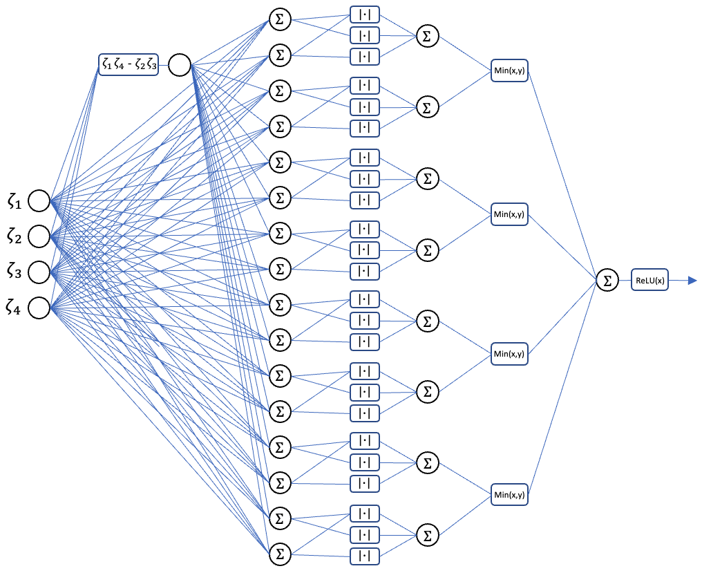
Our prior work in [3] developed a physics-based generative model that can generate all possible images containing runways $I_{r}(\xi)$ based on the physical parameters of the camera $f,\rho_{h},\rho_{w},v_{0},u_{0}$ (discussed in Section 2). Crucially, this physics-based generative model was shown to be mathematically equal to a change of coordinates $h:\mathbb{R}^{4}\rightarrow\mathbb{R}^{4}$ and a neural network $\mathcal{NN}_{r}(h(\xi))$ with carefully selected weights and parameters (this network is depicted in Figure 4), i.e.,

The change of coordinates $h$ maps the state of the aircraft into the projections of the endpoints of the lines L and R on the Pixel Coordinate Frame (PCF). For the sake of brevity, we defer the details of $h$ and $\mathcal{NN}_{r}$ to Appendix VI-A, and we refer the reader to [3] for detailed analysis of the correctness of this generative model.

Given a partitioning parameter $\delta$, we partition the state space $\Xi\subset\mathbb{R}^{4}$ into L regions $\Xi_{1},\ldots,\Xi_{L}$ such that each $\Xi_{i}$ is an infinity-norm ball with radius $\delta$. For each of these partitions, we aim to design a spatial filter that matches the spatial properties of the runway images that can be produced by states within such a partition. To that end, consider the following filter $\mathcal{S}^{\Xi_{i}}\in\mathbb{B}^{a\times b}$ defined as:

Recall that all images $I_{r}(\xi)$ are monochromatic (i.e., each pixel can take only a value of 0 or 1), then the following result follows directly from the definition above.

Note that the condition $\forall\xi\in\Xi_{i}.[I_{n}(\xi)\otimes\mathcal{NN}_{r}(h(\xi))=\mathbf{0}_{a,b}]$ is equivalent to $I_{n}(\xi)\otimes\mathcal{S}^{\Xi^{i}}=\mathbf{0}_{a,b}$. That is, the filter $\mathcal{S}^{\Xi_{i}}$ is capable of removing all noise in the image as long as the noise image $I_{n}(\xi)$ does not affect pixels that are $\delta/\rho_{w}$ away from the runway image $I_{r}(\xi)$. Figure 5 shows an example of such a filter. Specifically, equations (11)-(12) imply that the filter will accurately process the filtered image, provided that the noise does not resemble the pattern of runways. Additionally, the filter must be applied to the specific region corresponding to the state responsible for generating such a runway. Furthermore, it is reasonable to assume that as we increase the geometric complexity of the runway, the likelihood of noise resembling runway patterns diminishes. In other words, the more intricate the entity we are examining, the safer it is to rely on our assumptions.

What is remaining is to provide an algorithm that can compute the filter $\mathcal{S}^{\Xi_{i}}$ for each partition $\Xi_{i}$. Thanks to the fact that the physics-based generative model $\mathcal{NN}_{r}(\xi)$ is captured as a neural network, one can use output reachability algorithms to compute an overapproximation of the reach set (set of all possible images) for the runway image $I_{r}(\xi)$. For that end, we leverage Mixed-monotonicity reachability analysis of neural networks [15] by leveraging the following result:

To implement the method in Proposition 2, we define the input vectors as $\overline{\zeta}=\text{center}(\Xi_{i})+\frac{\delta}{2}$ and $\underline{\zeta}=\text{center}(\Xi_{i})-\frac{\delta}{2}$. Additionally, we compute the bounds on the Jacobian matrix of the neural network $\mathcal{NN}_{r}$ to find the bounds $[\underline{J},\overline{J}]$. Details about obtaining such bounds are given in Appendix VI-B. These bounds on the output of $\mathcal{NN}_{r}$ identifies which pixels are equal to zero for all the images generated by the states in each $\Xi_{i}$, which can be used to compute the filters in (10).

The spatial filters $\mathcal{S}^{\Xi_{i}}$ can be used to focus the attention on different regions of the state space. Although these filters provide a guarantee of the output of the filter that satisfies $\xi\in\Xi_{i}$ it does not provide any guarantee on the output of the filters for which $\xi\notin\Xi_{i}$. Therefore, it is necessary to augment the spatial filters with another filter that aims to detect whether the output follows the geometrical structure of the runway images. To achieve this, consider the following filters:

Such filter can be efficiently computed using the classical Hough-space transformation [16]. In this transformation, a straight line is represented by a normal line that passes through the origin and is orthogonal to that straight line. The equation of the normal line is given by $\rho=\zeta_{1}\cos{(\theta)}+\zeta_{2}\sin{\theta}$, where $\rho$ is the length of the normal line and $\theta$ is the angle between the normal line and the x-axis of the Pixel Coordinate Frame. By using the projections of the endpoints of the runway lines edges obtained from $h(\xi)=[\zeta_{1},\zeta_{2},\zeta_{3},\zeta_{4}]$ as $P_{1}=(\zeta_{1},\zeta_{2})$ and $P_{2}=(\zeta_{3},\zeta_{4})$, we can solve for $\theta$ and $\rho$ for the generated image as:

Given a partition $\Xi_{i}$, we can obtain the range of $\rho$, $\theta$ for all runway images as follows. First, recall that each partition $\Xi_{i}$ is an infinity ball with a radius equal to $\delta$ around a center point $\text{center}(\Xi_{i})\in\mathbb{R}^{4}$. The two points $P_{1}=(\text{center}(\Xi_{i})_{[1]},\text{center}(\Xi_{i})_{[2]})$ and $P_{2}=(\text{center}(\Xi_{i})_{[3]},\text{center}(\Xi_{i})_{[4]})$ represent 2-dimensional points in the Pixel Coordinate Frame that corresponds to the center of $\Xi_{i}$ (see Figure 6 for illustration). Following the 2-dimensional geometry of the Pixel Coordinate Frame, it is direct to show that:

where $m,\overline{b}_{\delta},\underline{b}_{\delta}$ are defined in Appendix VI-C.

Equations (18)-(22) define the reachable set of the runway images within the Hough space (the $\rho-\theta$ space). Moreover, the discretization introduced in the Pixel Coordinate Frame (the flooring operation in (2)) introduces a discretization over the range of $\rho$ and $\theta$ computed by equations (18)-(22) which existing implementations of Hough transformation algorithms take into account. We denote by $\mathcal{L}^{\Xi_{i}}=\{(\rho^{\Xi_{i}}_{max},\theta^{\Xi_{i}}_{\max}),\ldots,(\rho^{\Xi_{i}}_{min},\theta^{\Xi_{i}}_{min})\}$ the discrete set of the allowable values of $\rho$ and $\theta$ within the partition $\Xi_{i}$. For each possible $(\rho_{j},\theta_{j})$ in $\mathcal{L}^{\Xi_{i}}$, we define the filter $\mathcal{R}^{\Xi_{i}}(\rho_{j},\theta_{j})\in\mathbb{B}^{a\times b}$ as:

For each filter $\mathcal{R}^{\Xi_{i}}(\rho_{j},\theta_{j})$ we can define a mismatching score that computes how far the input image $I$ is from the expected output of this filter as:

That is, $\mathcal{M}$ is equal to zero whenever the input image $I$ matches exactly the line represented by $\mathcal{R}^{\Xi_{i}}(\rho_{j},\theta_{j})$ and non-zero otherwise. Finally, we can implement the filter $\mathcal{H}^{\Xi_{i}}$ in (15) as:

In other words, the filter $\mathcal{H}^{\Xi_{i}}$ produces 1 whenever any of the filters $\mathcal{R}^{\Xi_{i}}(\rho^{\Xi_{i}}_{max},\theta^{\Xi_{i}}_{max}),\ldots,\mathcal{R}^{\Xi_{i}}(\rho^{\Xi_{i}}_{min},\theta^{\Xi_{i}}_{min})$ were able to match its input image. The following proposition follows directly from the definition of $\mathcal{H}^{\Xi_{i}}(I)$ above.

The final filter $\mathcal{NN}_{F}$ consists of processing the images $I$ using all the spatial filters $\mathcal{S}^{\Xi_{1}},\ldots,\mathcal{S}^{\Xi_{l}}$ followed by the geometric filters $\mathcal{H}^{\Xi_{1}},\ldots,\mathcal{H}^{\Xi_{l}}$. Finally, the filter $\mathcal{NN}_{F}$ identifies the partition $\hat{\Xi}$ for which the geometric filter returns $1$ to produce its final outputs as follows:

The following result captures the correctness of the $\mathcal{NN}_{F}$.

Before we conclude this section, it is essential to interpret the assumptions (29) and (30) in Theorem 1. In particular, the assumption in (29) entails that the noise $I_{n}$ can not be generated using the runway generative model $\mathcal{NN}_{r}$. In other words, this assumption ensures that the noise does not look like a runway and hence only one image of the runway exists in the scene. The assumption in (30) asks that the pixels that are $\delta$ close to the runway are not affected by the noise. It is crucial to note that assumption (30) is required to be satisfied in $\Xi^{*}$ only and does not affect other partitions.

The generative model is made of two components: A change of coordinates $h$ and a ReLU-based Neural Network for Line Generation $\mathcal{NN}_{r}$ as captured by the following definitions.

In other words, the pair $(\zeta_{1},\zeta_{2})$ is the projection of the start point of the runway $(L_{x},0,L_{z})$ onto the Pixel Coordinate Frame PCF (while ignoring the flooring operator for now). Similarly, the pair $(\zeta_{3},\zeta_{4})$ is the projection of the endpoint of the runway $(L_{x}+r_{w},0,L_{z}+r_{L})$ onto the PCF frame. Indeed, we can define a similar set of variables for the other line segment of the runway, $R$. We refer to the new state space as $\Xi$.

We compute the bound on the Jacobian matrix of the Runway Generative Model as follows:

References

- [1] J. Ferlez, M. Elnaggar, Y. Shoukry, and C. Fleming, “Shieldnn: A provably safe nn filter for unsafe nn controllers,” arXiv preprint arXiv:2006.09564, 2020.
- [2] M. Alshiekh, R. Bloem, R. Ehlers, B. Könighofer, S. Niekum, and U. Topcu, “Safe reinforcement learning via shielding,” in Proceedings of the AAAI Conference on Artificial Intelligence, vol. 32, 2018.
- [3] U. Santa Cruz and Y. Shoukry, “Nnlander-verif: A neural network formal verification framework for vision-based autonomous aircraft landing.” NASA Formal Methods. NFM 2022. Lecture Notes in Computer Science, vol 13260. Springer, pp 213–230, 2022.
- [4] X. Sun, H. Khedr, and Y. Shoukry, “Formal verification of neural network controlled autonomous systems.” HSCC 19: Proceedings of the 22nd ACM International Conference on Hybrid Systems: Computation and Control, pp 147–156, 2019.
- [5] C. Hsieh, Y. Li, D. Sun, K. Joshi, S. Misailovic, and S. Mitra, “Verifying controllers with vision-based perception using safe approximate abstractions.” IEEE Transactions on Computer-Aided Design of Integrated Circuits and Systems, vol. 41, 2022.
- [6] S. M. Katz, A. L. Corso, C. A. Strong, and M. J. Kochenderfer, “Verification of image-based neural network controllers using generative models,” Journal of Aerospace Information Systems, vol. 19, no. 9, pp. 574–584, 2022.
- [7] P. Habeeb, N. Deka, D. D’Souza, K. Lodaya, and P. Prabhakar, “Verification of camera-based autonomous systems,” IEEE Transactions on Computer-Aided Design of Integrated Circuits and Systems, 2023.
- [8] R. Talak, L. Peng, and L. Carlone, “Certifiable 3d object pose estimation: Foundations, learning models, and self-training,” 2023.
- [9] S. Shoouri, S. Jalili, J. Xu, I. Gallagher, Y. Zhang, J. Wilhelm, J.-B. Jeannin, and N. Ozay, “Falsification of a vision-based automatic landing system,” in AIAA Scitech 2021 Forum, p. 0998, 2021.
- [10] H.-D. Tran, X. Yang, D. Manzanas Lopez, P. Musau, L. V. Nguyen, W. Xiang, S. Bak, and T. T. Johnson, “Nnv: the neural network verification tool for deep neural networks and learning-enabled cyber-physical systems,” in Computer Aided Verification: 32nd International Conference, CAV 2020, Los Angeles, CA, USA, July 21–24, 2020, Proceedings, Part I, pp. 3–17, Springer, 2020.
- [11] J. Ferlez and Y. Shoukry, “Polynomial-time reachability for lti systems with two-level lattice neural network controllers,” IEEE Control Systems Letters, 2022.
- [12] H.-D. Tran, D. Manzanas Lopez, P. Musau, X. Yang, L. V. Nguyen, W. Xiang, and T. T. Johnson, “Star-based reachability analysis of deep neural networks,” in Formal Methods–The Next 30 Years: Third World Congress, FM 2019, Porto, Portugal, October 7–11, 2019, Proceedings 3, pp. 670–686, Springer, 2019.
- [13] Y. Ma, S. Soatto, J. Kosecka, and S. S. Sastry, An invitation to 3-d vision: from images to geometric models, vol. 26. Springer Science & Business Media, 2012.
- [14] R. Hartley and A. Zisserman, “Multiple view geometry in computer vision,” Cambridge University Press, 2003.
- [15] P.-J. Meyer, “Reachability analysis of neural networks using mixed monotonicity.” IEEE Control Systems Letters,vol. 6, pp. 3068-3073, 2022.
- [16] R. Szeliski, Computer Vision - Algorithms and Applications, Second Edition. Texts in Computer Science, Springer, 2022.
VI Appendix
VI-A Physics-Based Generative Model