Fisher’s Pioneering work on Discriminant Analysis and its Impact on AI Based on “The 40th Fisher Memorial Lecture” delivered in November 2022, Oxford. Fisher died 60 years ago and this paper marks the anniversary of his death. For a link to the talk,
Abstract
Fisher opened many new areas in Multivariate Analysis, and the one which we will consider is discriminant analysis. Several papers by Fisher and others followed from his seminal paper in 1936 where he coined the name discrimination function. Historically, his four papers on discriminant analysis during 1936-1940 connect to the contemporaneous pioneering work of Hotelling and Mahalanobis. We revisit the famous iris data which Fisher used in his 1936 paper and in particular, test the hypothesis of multivariate normality for the data which he assumed. Fisher constructed his genetic discriminant motivated by this application and we provide a deeper insight into this construction; however, this construction has not been well understood as far as we know. We also indicate how the subject has developed along with the computer revolution, noting newer methods to carry out discriminant analysis, such as kernel classifiers, classification trees, support vector machines, neural networks, and deep learning. Overall, with computational power, the whole subject of Multivariate Analysis has changed its emphasis but the impact of this Fisher’s pioneering work continues as an integral part of supervised learning in Artificial Intelligence.
Keywords: Canonical variates, Classification, Genetic discriminant, iris data, Linear discriminant function, Machine learning, Mardia’s measures of skewness and kurtosis, Visualising multivariate data
1 Introduction
We begin with a quotation from Rao 1964; Rao was one of Fisher’s PhD students. He has summarised succinctly the pioneering work of Fisher in Multivariate Analysis as follows:
“Not much was known in the field of Multivariate Analysis by way of theory or applications before Fisher did his pioneering researches. Many important contributions by others have also been inspired by his work. He has forged a number of important tools and demonstrated their use in applied research, specially in the field of biology, all of which are ’bound to stay on the books and be used continuously’. Truly he was the architect of Multivariate Analysis …”
Modern computational advances have gone on to provide many extensions of Fisher’s work in Multivariate Analysis. We will discuss his pioneering work in discriminant analysis and its impact on statistical learning /AI.
Fisher 1936 paper is the landmark paper in discriminant analysis.
In his collected papers Fisher 1950 includes his commentary on this paper,
“This was written to embody the working of a practical numerical
example arising in plant taxonomy, in which the concept of a discriminant
function seems to be of immediate service.”
Fisher’s 1936-1940 papers
Fisher published four articles on statistical discriminant analysis between 1936 and 1940, namely
Fisher 1936,
Fisher 1938,
Fisher 1939, and
Fisher 1940.
In the first of these (Fisher 1936), he introduced and applied the Linear
Discriminant Function (LDF) (the Fisher’s Rule);
Fisher also considered the problem of classification and its connection with
regression analysis, including introduction of dummy variables.
Fisher 1936 dealt mostly with results needed for the comparison of three species of Iris, illustrated on the now-celebrated iris data.
The question posed by Fisher was
“What linear function of the four measurements
will maximize the ratio of the difference between the specific means to the standard deviation within species?”
and then it says in the paper “The particular linear function which best discriminates the two species will be one for…”,
and the subject of Discriminant Analysis/ Statistical Learning was borne.
Fisher 1938 reviewed his 1936 work and relates it to Hotelling’s , Mahalanobis and Hotelling’s Canonical Analysis. Also, he corrected his earlier significance test, pointing out
differences with the usual normal-theory regression.
The second half of this paper contains an attempt to extend the earlier work
to the case of populations.
The treatment is somewhat incomplete in Fisher 1938, but is completed
in Fisher 1939 and
Fisher 1940 and in his collected papers Fisher 1950.
Iris Data
Fisher 1936 published the full iris data, for the first time. The data were collected by
E. Anderson 1935, with further details in E. Anderson 1936, but the full data published by Fisher
is not included in either of the two papers by E. Anderson. The iris data has variables
= sepal length, = sepal width,
= petal length, = petal width,
and sample size from each of populations, three species of Iris
the measurements are in cm. For the data, see for example, Fisher 1936, Mardia et al. 2023, and in R: library(datasets), data(iris). Recently, Unwin and Kleinman 2021 have provided more sources on where to find this data.
Let be the respective data matrices, where . The sample means are given in Table 1.
| Sepal | Petal | ||||
| Length | Width | Length | Width | ||
| setosa | 5.006 | 3.428 | 1.462 | 0.246 | |
| versicolor | 5.936 | 2.770 | 4.260 | 1.326 | |
| virginica | 6.588 | 2.974 | 5.552 | 2.026 | |
Let and be the random vectors for the three respective populations and let with means and covariance matrices respectively. We will indicate if and when the normality assumption is used.
The flowers of the first two iris species
(setosa and versicolor) were taken from the same natural colony but the sample of the third iris species (virginica) is from a different colony.
One of the aims is to discriminate the three iris species based on the data.
Unwin and Kleinman 2021 seem to have recently traced the source of this data set, and their paper also gives a colour picture of these three flowers.
We now outline the contents of this paper which are mostly related to topics in Fisher’s 1936 paper and its subsequent development. Section 2 assesses his assumption of multivariate normality for the iris data. In Section 3, we carry out discriminant analysis for all the three iris populations via canonical variates but the technique of canonical variates arrived after Fisher 1936 which basically deals with two-population discrimination. New methods have appeared since to provide classification regions and in Section 4 for the iris data with two selected variables, we compare Fisher’s discriminant rule and the related maximum likelihood rule to two non-parametric methods: kernel classifier and classification trees.
When Fisher wrote his paper of 1936, he had the discriminant method for 2 populations but there were 3 populations in the iris data. This he handled by going into the so-called genetic hypothesis of the iris data, which led to his specific analysis. The construction to handle the hypothesis took him to a new rule for discrimination, but this construction is not well understood as far as we know. We give some rationale behind his rule, which we call “genetic discriminant”, in Section 5. In his 1936 paper, Fisher gave an effective way to plot classification histograms of his genetic discriminant and in Section 6 we examine some modern multivariate visualisations of the various discriminants. Matrix algebra is one of the most important mathematical tools in statistics and especially in multivariate analysis. Fisher used some matrix algebra in Fisher 1936, but overall matrix algebra came slowly into use; there was some resistance in the 1940’s. We give a very brief history on the appearance of matrix algebra in multivariate analysis in Section 7. Finally, Section 8 gives a short overview of how Fisher’s discriminant analysis has influenced the field of supervised learning which is an integral part of AI .
2 Testing Multi-normality of the Iris Data
Initially, Fisher 1936 sets up the problem without the need to assume any distributions, but for calculating the classification error, he says, ”We may, therefore, at once conclude that if the measurements are nearly normally distributed …”. Subsequently, for testing genetical hypothesis he again assumes normality.
We now assess this assumption. For this section, we use the notation that is a random sample from a population in dimensions with the sample mean vector and sample covariance matrix . Using the invariant functions
Mardia 1970 introduced the following multivariate measures of skewness and kurtosis respectively.
Some of the attractive properties of these measures are:
- (1)
For the univariate case, and , so these reduce to the standard measures where the ’s are univariate central moments.
- (2)
depends only on the moments up to the third order, whereas only on the even moments up to the fourth order.
- (3)
These measures are invariant under affine transformations.
- (4)
For the multivariate normal distribution, the population measures have values
- (5)
Under normality, and , have the following asymptotic distributions
These statistics are used to test the null hypothesis of multivariate normality for large samples. For small samples, Mardia 1974 has given critical values of these statistics.
- (6)
These measures are available in all the standard statistical packages and are now one of the most popular measures.
| setosa | versicolor | virginica | |
| skewness | 3.1 (25.7) | 3.0 (25.2) | 3.2 (26.3) |
|---|---|---|---|
| kurtosis | 26.5(1.3) | 22.9 (0.6) | 24.3(0.2) |
We have under normality, the population values are and so it can be seen from the Table 2 that the species have similar skewness and kurtosis values as for the multivariate normal. Further, the value for is 31.41 with , and the value for is 1.96. So, it can be seen from Table 2 that skewness and kurtosis values are not significant at the level of significance. Hence, Fisher’s assumption of multivariate normality for the iris data is justified by these measures.
3 Canonical Variates
Suppose ( are data matrices where represents the data matrix a sample of size on variables from
population , .
The task of discriminant analysis is to allocate a new observation to
one of these populations.
Fisher’s approach was to look for the linear function
that maximizes the ratio of the between-groups sums of squares and cross products matrix to the within-group sums of
squares and cross products matrix ; that is, is the vector which maximizes
| (1) |
It can be shown that the vector is the eigenvector of
corresponding to the largest eigenvalue, normalised as in the above expression (1); see, for example, Mardia et al. 2023. This tractable practical solution was provided by Bryan 1951.
Classification Rule I.
Let be the th sample mean vector, . Allocate to if
Canonical Analysis of Iris Data
In general, has non-zero eigenvalues, and its eigenvectors
define the first, second and subsequent “canonical variates”; the first canonical
variates summarize the difference between
the groups in dimensions. Note that the first canonical variable provides the discriminant for 3 populations.
Mardia et al. 1979 pp.344-345 have given the first two canonical variables for the iris data as
| (2) |

Figure (1) plots these first two canonical variates for the data, with their 99 probability region together with their canonical means. The figure shows that the three species are different but there is some overlap between virginica and versicolor.
| Actual | |||||
|---|---|---|---|---|---|
| setosa | versicolor | virginica | Total | ||
| Predicted | setosa | 50 | 0 | 0 | 50 |
| versicolor | 0 | 48 | 0 | 48 | |
| virginica | 0 | 2 | 50 | 52 | |
| Total | 50 | 50 | 50 | 150 | |
4 Classification Regions for the iris data with two variables
Recall, we have three iris species each with the sample size and there are four variables . For illustrative purpose, we have selected the first two variables, sepal length, and sepal width. The choice of also helps with visualization; see also Section 6. Recall further that the first two iris species setosa and versicolor were taken from the same colony but the sample of the third iris species virginica differ as it was not taken from the same natural colony.
We give the classification regions, and thus the allocation of each observation to one of three species, for two parametric methods
(1) Fisher’s linear discriminant or the Fisher Rule, Figure 2 and
(2) maximum likelihood discriminant (equal covariances) or the ML Rule, Figure (2),
and two new statistical learning methods which are non-parametric:
(3) a kernel classifier, Figure 3 and
(4) a classification-tree classifier, Figure 4.


Some comments on the iris data
We have applied four methods of discrimination/ statistical learning to classify the iris data (by two variables). The classification regions are similar though some boundaries are curved rather than straight lines.
The Fisher Rule and the kernel classifier allocations agree for 132 of 150 observations, and the Fisher Rule and classification-tree allocations also agree for 132 of 150. (The two sets of 132 observations are not identical.). Whereas, the ML Rule and the kernel classifier agree in 139 of 150 observations in allocations, and the ML Rule and the classification-tree agree in 141 of 150. Thus the classification methods are similar on this basis as well.
The correct classification (prediction) rates are for (1) the Fisher Rule 117 of 150 (2) the ML Rule, 120 of 150, (3) the kernel classifier 127 of 150, and for (4) the classification-tree classifier, 119 of 150. These prediction rates are all based on re-substitution.
Thus the method are very similar on this basis as well. In fact, Shinmura 2016 compares 8 different linear discriminant functions (LDFs) using several different types of data sets including the iris data. The author asserts (p. 53) that “Because there are small differences between Fisher’s LDF and other LDFs, we should no longer use iris data as the evaluation data.” Thus even using only two variables, the allocation results are similar. This is expected since the three samples pass the test of multivariate normality (Section 2) as under normality the Fisher rule is optimal when all the variables are used.
5 Fisher’s genetic discriminant
5.1 Intoduction
Fisher 1936 in his Section 6 constructed a genetic discriminant based on the reasoning described in his paper; see Figure 5 which reproduces an extract of his Section 6. He concluded that we should use the linear combination of the four measurements most appropriate for discriminating these 3 species when it is known (from genetic considerations) that the mean value for versicolor takes an intermediate value differing twice as much from setosa as from virginica, namely, versicolor has been formed as a 1:2 mixture of setosa and virginica.

That is, using our notation with the mean vectors , , and of setosa, versicolor, and virginica respectively, then
| (3) |
Fisher’s genetic discriminant takes into account this prior information with the aim to find the best linear combination of measurements separating the two putative parents (setosa and virginica), and then to test whether versicolor lies 1:2 between setosa and virginica on that combination. (see also, Figure 10 of E Anderson.)
We now attempt to justify this Fisher’s genetic discriminant. Since it pre-specifies a direction of the discriminant, we denote this linear discriminant function (LDF) in a pre-specified direction by LDF-PD.
Recall that when this paper was written, canonical variate analysis was not yet developed to carry out discrimination for more than two populations (3 populations here). Even then, it is worth finding out how Fisher successfully constructed a plausible discriminator. His reasoning is not explicit from the paper and he did not come back to it in his later writings, nor do any later researchers. On the other hand, Box 1978 points out that how crucial is this work under a pre-specified direction, see Figure 6.

The relationship of LDF-PD with canonical variates is examined in Section 5.3. In Section 5.4, we analyse the iris data using the LDF-PD and it is interesting to note that the Fisher’s genetic discriminant performs as good as the standard canonical variate discriminant; both only 2 observations misclassifying out of 150 observations. Finally, we formally test the hypothesis of the genetic relationship (3) in Section 5.5.
5.2 Derivation
Let us assume that we have populations with the random variables in dimensions with population means and covariances respectively. We assume that are all different but collinear. In Fisher’s derivation of LDF-PD three principles are involved and we first give an outline and later on each principle is expanded.
- 1.
Principle 1: Optimal contrast of population means Finding an optimal contrast of population means for which the groups are most different under given linear constraints on the (unknown) means. That is, to find the vector such that the following linear combination is optimal.
(4) The optimum criterion is given below at (12) with some constraints on . We denote the optimal by so that the optimal contrasts on the means is
(5) - 2.
Principle 2: Population Discriminant Using the resulting from Principle 1 form an “optimal” combination of the random variables
(6) For discrimination, consider the linear combination
(7) and the optimal creation is formed using the signal to noise ratio, namely
(8) Let the optimal value of be .
- 3.
Principle 3: Classification Rule II. Let be the new observation to be allocated. Using now , calculate the “discriminator function” and allocate to the th population if
(9) For this Classification Rule, it is assumed that all the populations parameters are known.
Note that these three principles are all related to the populations and not to samples from these populations except in Principle 3 where is an observation to be allocated. We now work through each of these three Principles in detail.
Principle 1: Optimum Contrasts of Population Means. We now obtain the optimum linear combination (5). Let us assume there are known linear constraints on the means, such as
| (10) |
where are some known constants. Further, we assume (see below for the rationale behind these constraints for the particular case of but the same argument extends for any .)
| (11) |
We define our criterion (optimum criterion) to be optimized is
| (12) |
where is the mean of the . The criterion measures the Euclidean distances between the means.
In the discussion, we assume that initially and restrict to the constrain (3) used by Fisher and then give an extension. (Note there is only one constraint in this case and is given in (3)). That is, our linear combination is of the form
| (13) |
and the means are constrained to
| (14) |
Using the collinearity of the , we can write
| (15) |
where represents the direction of species differences, is the aforementioned linear combination, and is a common translation vector. Without any loss of generality, we can take
| (16) |
by absorbing into where . Substituting (15) into (14) gives
| (17) |
or, since ,
| (18) |
From the two constraints (16) and (18), is given, up to a scaling constant, by
| (19) |
We now show that satisfies the optimal criterion given at (12). We have
| (20) |
where . We have where is a unit vector. Substituting this value of in (20), we get
Hence is maximum when is maximised so by the Cauchy–Schwarz inequality we have
Finally, we note that for , we need more known constraints, that is constraints to get a single optimum direction where for , the optimal linear combination is trivially
.
Principle 2: Optimum Linear Combination of Random Variables. Now we assume that the vector is known and we define the random vector
| (21) |
where the ’ s are distributed independently with the jth mean vector and the jth covariance matrix ; . So that
| (22) |
Let be the “discriminant” function where is a new observation we define the discriminant where by maximising with respect to the signal to noise ratio given at (8) in terms of so
| (23) |
A proof of (23) on maximising (8) can be derived using Corollary A.9.2.2 of Mardia et al. 1979.
Note that there is no assumption on but as the ‘s
are independent, so that though this rule does not assume equality of covariances.
The above formulation might look strange as at (6) is defined as a linear combination of random vectors representing different populations. Further, population discriminant using Fisher’s signal to noise ratio is mostly seen in the sample version. However, there are some exceptions. We describe here a particular case which Rao 1973 treated and Figure 7 gives an extract from Rao 1973 indicating how Fisher’s discriminant function can be formulated for two populations. In Rao’s case, in (6). He then used the signal to noise ratio (as we have done in (8) for our general case) to obtain his which is equivalent to our However, it is to be noted that in Rao’s case ’s are known and his case is only for what his Book required.

We restate
CLASSIFICATION RULE II
Allocate to the th population if
| (24) |
Note this rule is standard rule fro the sample case for the canonical variate discrimination and, for , it simply becomes
| (25) |
Indeed, so it does not depend on covariance matrices. However, this is different than the likelihood based rule and these take into account the differences in covariance matrices. Consider the univariate case with two populations: is the distribution, and is the distribution. Let and . Then maximum likelihood rule allocates new to if
| (26) |
Thus the rule takes into account that the ’s are different. Further, the set of the ’s for which this inequality
is satisfied forms two distinct regions, one having low values of and the
other having high values of . For , the rule is the same as the above Fisher’s rule.
Estimation. Given a sample, we get the sample discriminant function following Fisher’s idea, by plugging in the standard estimates of
, respectively in (23) so we have the coefficient vector
| (27) |
Now we can allocate new observation using the plugged in version of (24). We can extend to the ML rule under multivariate normality but this will be not pursued here.
5.3 Relation of LDF-PD with Canonical Variates
The LDF-PD given in Section 5.2 raises several questions including how the Classification Rule II relates to canonical variates. Here we give its relationship with canonical variates for a particular case of Let and be the within- and between-population matrices respectively.
| (28) |
| (29) |
For the eigenvector , we need to solve
| (30) |
where is an eigenvalue. We find that the first canonical variate, corresponding to the single non-zero eigenvalue , is
| (31) |
This is the same as in Fisher’s rule given by (23) when A proof of (31) follows on substituting this value of into (30) together with (29).
5.4 iris data
Now consider our iris case. As shown above at (13), the optimal linear combination and the corresponding random vector are given by
| (32) |
That is substituting in (23), the “genetic discriminant” is given by
| (33) |
The estimates of and , in (33), as done in (27), yield the estimated weight vector . It is found that is the genetic discriminant
| (34) |
Indeed, Fisher 1936 gave the discriminant (33) without any explanation. The confusion matrix for this discriminant is shown in Table 4.
Note that the only two errors, out of 150 predictions, are
to misallocate observations 71 and 84 (the numbering follows the order in the Fisher tabulated data) which belong to versicolor and are allocated to virginica.
| Actual | |||||
|---|---|---|---|---|---|
| setosa | versicolor | virginica | Total | ||
| Predicted | setosa | 50 | 0 | 0 | 50 |
| versicolor | 0 | 48 | 0 | 48 | |
| virginica | 0 | 2 | 50 | 52 | |
| Total | 50 | 50 | 50 | 150 | |
Fisher does not give a confusion matrix and his work was prior to the canonical variates as we have mentioned above in Section 3. Note that these both discriminant have the same confusion matrix but mistakes for observations 73 and 84 by canonical discriminant rather than 71 and 84 by the genetic discriminator and both from versicolor allocated “wrongly” to virginica.
In fact, the first canonical variable given at (2) normalised so the length is unity then it becomes
where as the normalised genetic discriminant is
which shows that these two are are very close and differ due to the original different normalisation.
It can be seen from the visual plots of the data that the covariances for the three populations are different (see also Figure 8) (can be tested formally by the Box M-test) but it is interesting that both lead to the same level of error though the canonical variates rule assume the equality whereas the Fisher genetic discriminate does not.
| Actual | |||||
|---|---|---|---|---|---|
| setosa | versicolor | virginica | Total | ||
| Predicted | setosa | 50 | 0 | 0 | 50 |
| versicolor | 0 | 48 | 1 | 49 | |
| virginica | 0 | 2 | 49 | 51 | |
| Total | 50 | 50 | 50 | 150 | |
For completeness, we give in Table 5, the allocations using the ML discriminant with all the four variables; recall that only two variables were used in Section 4). We note from the Table that 3 observations out of 150 are misclassified– 2 versicolor observations gets allocated to virginica and, one virginica to versicolor so the behaviour is very similar.
“Shape” Discriminants
Define
Anderson 1936 used the non-linear discriminant defined by
| (35) |
which he called it an Index for a basis for comparison. This is in some sense a “shape” discriminant. Fisher 1936 made no comment on this Index, perhaps as the two papers came out in the same year. If we use the E. Anderson Index as a discriminant, the confusion matrix is given in Table 6 so 11 observations are misclassified, namely 4 observations of setosa go to versicolor and 3 of virginica go to versicolor.
| Actual | |||||
|---|---|---|---|---|---|
| setosa | versicolor | virginica | Total | ||
| Predicted | setosa | 46 | 0 | 0 | 46 |
| versicolor | 4 | 46 | 3 | 53 | |
| virginica | 0 | 4 | 47 | 51 | |
| Total | 50 | 50 | 50 | 150 | |
If we use as the variables, it is found that the Fisher discriminant is
so the length ratio dominates rather than the width ratio. The confusion matrix for the two shape ratios is given in Table 7 so there are 8 observations misclassified, with 7 observations of versicolor go to virginica and 1 of virginica goes to versicolor so but so it is a bit better than the E. Anderson’s Index (11 observations are misclassified).
| Actual | |||||
|---|---|---|---|---|---|
| setosa | versicolor | virginica | Total | ||
| Predicted | setosa | 50 | 0 | 0 | 50 |
| versicolor | 0 | 43 | 1 | 44 | |
| virginica | 0 | 7 | 49 | 56 | |
| Total | 50 | 50 | 50 | 150 | |
Alternative to consider are the shape variables based on the two areas
If we use as the variables, it is found that the discriminant function is
The confusion matrix for the shape areas is given in Table 8 so there are 4 observations misclassified with 1 observation of versicolor go to virginica and 3 observations of virginica goes to versicolor.
| Actual | |||||
|---|---|---|---|---|---|
| setosa | versicolor | virginica | Total | ||
| Predicted | setosa | 50 | 0 | 0 | 50 |
| versicolor | 0 | 49 | 3 | 52 | |
| virginica | 0 | 1 | 47 | 48 | |
| Total | 50 | 50 | 50 | 150 | |
Thus the area variables do a bit better than the Index variables but the genetic discriminant and the canonical discriminant are marginally better. These shape discriminants have the advantage of using the two dimensional data summary so visualisation is simpler.
For completeness, let us go back to the two variables sepal length and sepal width we have used in Section 4. It is found that the canonical discriminant using these two variables is
so both and contribute. The confusion matrix is given in Table 9 and it can be seen that the classification errors are higher (30 misclassified now) much higher than the shape variables above (10 misclassified) with these two variables which is consistent that we need all the four variables.
| Actual | |||||
|---|---|---|---|---|---|
| setosa | versicolor | virginica | Total | ||
| Predicted | setosa | 49 | 0 | 0 | 49 |
| versicolor | 1 | 36 | 15 | 52 | |
| virginica | 0 | 14 | 35 | 56 | |
| Total | 50 | 50 | 50 | 150 | |
5.5 Testing of the Genetic Hypothesis
From our discussion in the beginning of this section we say that if versicolor takes an intermediate value such that it differs twice as much from setosa as from virginica then the null hypothesis from (3) is
Substituting the sample means from Table 1 into the genetic discriminant (34), we get , , , so . Note that Fisher 1936 denotes the first population as virginica, second as versicolor and third as setosa, and gives more decimal points. He gives =3.07052; var() =4.8365, SE() =2.199. As is large, we could use normal theory so the 95 confidence interval is (-1.33,7.47) and we accept the null hypothesis. Fisher points out that this test is not exact and does the correction but the conclusion is the same.
6 Visualisation
Fisher 1936 found a way to visualise the iris data by drawing histograms of his genetic discriminant given by (34) for the three populations (his Figure 1, reproduced here as Figure 8).

We have added some annotations to his Figure 1 in our Figure 8 (coloured boxes) as it depicts 4 important features as follows. (a) The histogram of versicolor when compared to the histogram of virginica and seotsa, it can be seen that there is overlap between the versicolor and virginica histograms. (b) There are just two observations of versicolor, in the green box on that histogram, that are not classified correctly, they are allocated to virginica, by the genetic discriminant. (c) On the top horizontal line in the figure the three mean values and the mean value for versicolor under the genetic hypothesis are plotted (thicker arrow in the red box); versicolor takes an intermediate value differing twice as much from setosa as from virginica; visual inspection indicates the plausibility of the null hypothesis. (d) The sample standard deviations for the genetic discriminant are (2.4, 4.2, 4.3) for setosa, versicolor, and virginica respectively and Fisher plots each cell of the histograms, corresponding to a single observation, of the ”histogram” for setosa with half the width of the cells in the histograms for versicolor and virginiica. Accordingly, to preserve area, the cells for setosa are each twice the height as indicted by the blue boxes for setosa and virginca histograms (versicolor and virginica have the same heights).
Interestingly, E. Anderson 1928 created what he called “Ideographs” which show all four variables at once by constructing a white rectangle with the length and the width for petal which is superimposed on a black rectangle with the same dimensions for sepal. Figure 9 shows these for typical virginica and versicolor observations. We can see the difference in comparing the two final rectangle that how the two species differs. E. Anderson 1928 was not only in touch with Fisher but also John Tukey and he took this ideograph representation further to allow for more features leading to “metroglyphs” an extension of glyphs. For more details, see Kleinman 2002. Note that the areas of the two rectangles (bivariate data) for visualisations of the full iris data have been used in a scatter plot by Wainer and Velleman 2001.

In fact, E Anderson 1936 created a 3-dimensional model of his ideographs for the iris data depicting his genetic hypothesis as reproduced in Figure 10. In the caption to this Figure, he refers to Figure 8 which is here Figure 9.

Following the concept of ideographs, a simple presentation, an alternative to Figure 9, is to construct “Stacked-Rectangle” plots of the mean vectors for each iris species with length along the y-axis and width along the x-axis. In Figure 11 we give such a plot with sepal measurements prescribe the top rectangles, with rectangles for petal below, with a common edge. It can be seen that setosa is very different from versicolor and virginica, and further that virginica is “bigger” than versicolor. Further, an alternative to the 3-dimensional model of the genetic hypothesis in Figure 10 of E. Anderson, we give our stacked rectangle version in Figure 12 using the observed means of versicolor for the solid rectangle and using the means of setosa and virginica into (3) computed for versicolor means under the hypothesis for the dotted rectangle. We can see clearly the closeness between the observed means and the “hypothesis” means for versicolor.


Chernoff face representations have been popular (see for example, Mardia et al. 1979, Chapter 1). Figure 13 shows three faces corresponding to the mean vectors of setosa, versicolor, and virginica; plotted using the R library aplpack with all four variables – sepal length and sepal width, petal length and petal width. Again, we note that the face associated with setosa looks quite different from the other two faces.

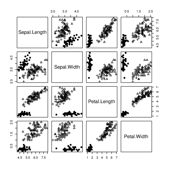
It has now become common to draw a set of 2D scatter plots or even a set of the perspective 3D plots in colour for higher dimensional data, both in print and utilizing visualization software. For the iris data, Figure 14 gives a scatter plot matrix. It is clear that setosa has no overlap with the other two species, but those two species (versicolor and virginica) do have overlap and for some variables, the overlap is more pronounced than for others.
Another approach is using class preserving plots as developed by Dhillon et al. 2002, which uses the first two principal components of the between sums of squares and cross products matrix . Here, we have
the first principal component , and
the second principal component ,
with eigenvalues ,
so all the information is in two dimensions. Figure 15 gives the PCA plot. In this one 2D plot, one can visualise the differences among the three species more vividly.
We have already given a plot using the first two canonical variables (using ) in Figure 1. But , the within sums of squares and cross products matrix can be singular for high dimensional data so working with is preferred for visualisation.

In general, computing packages have made the visualisation of multivariate data much easier, including 2D and 3D scatter plots of raw data and derived components eg canonical variates, and also visualization using interesting alternatives, e.g., Chernoff’s faces and Andrews’ function plots (see Mardia et al. 2023 for examples). Still there are visualisation tools described in the literature that have yet to catch on, such as those described in the papers by Tukey and Tukey 1981a, Tukey and Tukey 1981b and Tukey and Tukey 1981c. However for printed publication, 2D representations (sometimes in colour) remain the most popular tool.
7 A Very Brief History of the Appearance of Matrix Algebra in Multivariate Analysis
Matrix algebra is one of the most important mathematical tools in statistics and in particular in multivariate analysis. We give here a brief history, tracing the historical appearance of matrix algebra in the statistic literature. Our treatment follows David 2006, and the very recent Bingham and Krzanowski 2022 (seems to be written independently of the earlier David 2006 paper) .
Fisher relied on the power of -dimensional geometry in his research work and avoided matrix algebra. From the following comment in Fisher 1939, his preference is clear. “The paper incorporates the solution of the simultaneous distribution. of the latent roots which arise in discriminant analysis, without the formidable notation of matrix algebra. The method of resolution of this rather difficult problem may therefore be of interest in view of other possible applications.”
However, Fisher does use matrix algebra and matrix terminology. Even in Fisher 1936, the title of one of his tables reads “Table IV. Matrix of multipliers reciprocal to the sums of squares and products within species ().”
According to David 2006, the first appearance of matrix algebra in a statistics book seems to be in Turnbull and Aitken 1932. They gave the multivariate normal density in completely modern notation, eg Figure 16. According to David 2006, credit for the introduction of matrix algebra into statistics must go to A. C. Aitken for the book cited and his earlier paper, Aitken 1931. Surprisingly, Aitken did not use matrices in his book “Statistical Mathematics”, Aitken 1939, and later editions.

Matrix algebra begins to make fairly frequent appearances in the 1940’s, though not without some resistance. Cramér 1946 has a chapter introducing matrices which he then uses in subsequent chapters. Bartlett in his seminal discussion paper Bartlett 1947 writes, seemingly defensively, “Perhaps I should add that while I have avoided any complicated analytical discussion of theoretical problems, I have not hesitated on occasion to refer to the mathematical theory, with the aid of matrix and vector algebra or associated geometrical representation.”
During my discussion of the autobiography of George Box published in 2013 Box 2013, David Cox mentioned to me that Box in his BSc degree examination used matrix algebra to answer a question on the linear model and the examiner Florence David gave him poor marks for using matrix algebra, even though the answer was perfectly correct. George Box obtained his BSc degree in mathematical statistics from University College London in 1947, and Florence David was a member of staff of the Statistics Department there from 1945-1962.
In the 1950’s, matrix algebra became well established in multivariate analysis with the books of Rao 1952 and Anderson 1958, and subsequently the extensive Rao 1965 (second edition Rao 1973). Sen 1987 points out in discussion to Schervish 1987, itself a review of the second edition of Anderson’s book, “It is undoubtedly true that a generation of (mathematical) statisticians (specially, in the North American continent) has been raised on the classical (1958) textbook of T. W. Anderson, An Introduction to Multivariate Statistical Analysis”.
In fact, Cramer and Darell Bock 1966 in their review of Multivariate Analysis give another assessment. “The standard reference in multivariate analysis is undoubtedly Anderson’s (1958) book, An Introduction to Multivariate Analysis, but its high difficulty level and the paucity of examples make it an unsuitable reference for the research worker. Rao’s (1952) book remains an important reference for the research worker, with its emphasis on applications of discriminant theory; his later work (1965a) has some overlap in the multivariate analysis area but is at a higher mathematical level.” Rao’s (1965a) cited here in this quote is Rao 1965.
Indeed, the book by T.W. Anderson (Anderson 1958) on Multivariate Analysis (with various editions) is a classic, and it is interesting to note that he started his work in the field as a Ph.D student reading the Fisher’s papers on discriminant analysis (see his description in Figure 17).

On a personal note, in my two-year M.Sc. course in Statistics from Bombay University in 1955-1957 we used the celebrated Kendall’s volumes, Kendall 1948 and Kendall 1951, as well as Cramér 1946 and Rao 1952. At that time the pioneering books devoted solely on multivariate analysis, Kendall 1957 and Anderson 1958, were not yet published. Professor Kshirsagar was one of my teachers; subsequently he wrote his influential book Kshirsagar 1972 in multivariate analysis.
Bingham and Krzanowski 2022 point out that the crux for the formulae for the multivariate normal density lies with the papers by Edgeworth in 1892-3, and Stigler 1986, Chapter 9, pp 322-325, calls this Edgeworth’s theorem. However, the matrix notation for the multivariate density as used now is due to Aitken as described above though it is with the concentration matrix and not the covariance matrix. On the other hand, his joint book (Turnbull and Aitken 1932) does derive the second order moments. We refer for more details to the papers of David 2006 and Bingham and Krzanowski 2022.
8 Statistical Learning and AI
Learning problems in multivariate analysis can broadly be classified into two groups, supervised learning and unsupervised learning. In supervised learning, the goal is the same as in discriminant analysis whereas in unsupervised learning, the goal is the same as in cluster analysis. More details on this topic can be found in Efron and Hastie 2016, Hastie et al. 2009 and Mardia et al. 2023. In modern techniques in these areas, computation plays a key role. Note that discriminant analysis is also known as classification, pattern recognition, machine learning or statistical learning though the emphasis might differ.
In particular, to quote Sharma and Kaur 2013 “Pattern Recognition is one of the very important and actively searched trait or branch of artificial intelligence. It is the science which tries to make machines as intelligent as human to recognize patterns and classify them into desired categories in a simple and reliable way.” Indeed, with recent overwhelming interest in AI, there have been general questions on how important is the role of statistics. For example,Faes et al. 2022 have pointed out “The research on and application of artificial intelligence (AI) has triggered a comprehensive scientific, economic, social and political discussion. Here we argue that statistics, as an interdisciplinary scientific field, plays a substantial role both for the theoretical and practical understanding of AI and for its future development. Statistics might even be considered a core element of AI.” Also, it is to be noted that the terms used in the statistical vs. machine learning/AI world are not in general the same and Faes et al. 2022 have provided a table giving one to one correspondence between the two areas. Ghahramani 2015 has also given an excellent review on statistical learning and artificial intelligence.
We have already described Fisher’s linear discriminant function. It can be viewed as an intuitive approach to discriminant analysis that looks for a “sensible” rule to discriminate between populations. It relies on the means and covariances, and one of its extensions has been to take the populations as normal.
Alternative nonparametric methods are also available; some are given in Section 4. The simplest of these methods, -nearest neighbour, allocates a new observation according to a majority vote among the labels of the nearest neighbours in the data to .
Other nonparametric methods use recursive partitioning. As the name suggests, this method successively divides the data into subdivisions. Each partition corresponds to a rule based on an inequality for a one-dimensional function of the attribute data , for example, . The choice of partition depends on the purity (which uses the associated labels) of the data in each resulting subdivision. We can describe this process by a sequence of rules, usually based on components of , and these can be represented as a classification (or decision) tree. Some recent approaches, for example ensemble methods, boosting, and random forests, are closely connected to classification trees. Many of such methods are more algorithmic than model-based.
Logistic regression also makes few assumptions about the distribution of the data. Some recent approaches include neural network / deep learning families of algorithms, utilizing multi-layer perceptrons, of which logistic regression represents a simple case, radial basis functions and support vector machines. These have all been widely used for discriminant analysis.
However, the area of machine / statistical learning is very broad, and extends beyond multivariate analysis to many fields of statistics, such as spatial analysis (see Kent and Mardia 2022). The original motivation for neural networks to mimic the possible learning behaviour of the human brain is now considered part of neuroscience in AI, connected by statisticians to discriminant analysis. It seems Brian Ripley was the first to make that connection in a series of papers (see, for example, Ripley 1994). In particular the iris data, as an early example of illustrating neural networks, has been used in Ripley 1994.
It is important to note that the aim of discriminant analysis is to find a rule to separate distinct populations, and then to use that rule (or a different classification scheme) to allocate a new observation to the given populations. Fisher 1936 has both these elements. In the initial sections he developed how to form a discriminant rule and subsequently, in his Figure 8, he carried out his classification using the genetic discriminant. Of course, that is just one method to carry out classification.
Friedrich et al. 2022 have stressed that “The objective of statistics related to AI must be to facilitate or enable the interpretation of data. As Pearl puts it: ‘Data alone are hardly a science, regardless how big they get and how skillfully they are manipulated’ (Pearl 2018). What is important is the knowledge gained that will enable future interventions.” We conclude with the following important message in Faes et al. 2022 “Fundamental work on ML goes back to the 1960s and was developed on the basis of mathematical and statistical principles to which traditional statistics also refers (Foote 2021). It is worth remembering its roots.” (Here ML stands for Machine Learning.)
Remarkably, one of the leading pioneers in AI, Stephen Wolfram, has summarised his vision succinctly in Wolfram 2023: “For decades there’s been a dichotomy in thinking about AI between “statistical approaches” of the kind ChatGPT uses, and “symbolic approaches” that are in effect the starting point for WolframAlpha. But now —thanks to the success of ChatGPT—as well as all the work we’ve done in making WolframAlpha understand natural language—there’s finally the opportunity to combine these to make something much stronger than either could ever achieve on their own.”
Undoubtedly, the Fisher Rule is the first statistical rule for discrimination. It plays a major role in supervised learning and is the foundation more generally of AI.
9 Acknowledgements
The author is grateful to Colin Goodall, John Kent, Wojtek Krzanowski, Charles Taylor and Xiangyu Wu for their helpful comments and to the Fisher Memorial Trust for inviting me to give the talk. Thanks are also due to the Leverhulme Trust for the Emeritus Fellowship.
References
- Aitken (1931) Aitken, A. C. (1931) Some applications of generating functions to normal frequency. The Quarterly Journal of Mathematics, os-2, 130–135.
- Aitken (1939) — (1939) Statistical Mathematics. Edinburgh and London: Oliver and Boyd.
- Anderson (1928) Anderson, E. (1928) The problem of species in the northern blue flags, iris versicolor l. and iris virginica l. Annals of the Missouri Botanical Garden, 15, 241–332.
- Anderson (1935) — (1935) The irises of the Gaspé Peninsula. Bull Am Iris Soc, 59, 2–5.
- Anderson (1936) — (1936) The species problem in iris. Ann. Missouri Bot. Gard., 23, 457–509.
- Anderson (1958) Anderson, T. W. (1958) Introduction to Multivariate Statistical Analysis. Wiley.
- Anderson (1996) — (1996) R. A. Fisher and multivariate analysis. Statistical Science, 11, 20–34.
- Bartlett (1947) Bartlett, M. S. (1947) Multivariate analysis. Supplement to the Journal of the Royal Statistical Society, 9, 176–197.
- Bingham and Krzanowski (2022) Bingham, N. H. and Krzanowski, W. J. (2022) Linear algebra and multivariate analysis in statistics: development and interconnections in the twentieth century. British Journal for the History of Mathematics, 37, 43–63.
- Box (2013) Box, G. E. P. (2013) An Accidental Statistician: The Life and Memories of George E. P. Box. Wiley.
- Box (1978) Box, J. F. (1978) R A Fisher, The Life of a Scientist. Wiley, New York.
- Bryan (1951) Bryan, J. G. (1951) The generalized discriminant function: mathematical foundation and computational routine. Harvard Educational Review, 21, 90–95.
- Cramer and Darell Bock (1966) Cramer, E. M. and Darell Bock, R. (1966) Multivariate analysis. Review of Educational Research, 36, 604–617.
- Cramér (1946) Cramér, H. (1946) Mathematical Methods of Statistics. Princeton University Press.
- David (2006) David, H. A. (2006) The introduction of matrix algebra into statistics. The American Statistician, 60, 162–162.
- Dhillon et al. (2002) Dhillon, I. S., Modha, D. S. and Spangler, W. S. (2002) Class visualization of high-dimensional data with applications. Computational Statistics and Data Analysis, 41, 59–90.
- Efron and Hastie (2016) Efron, B. and Hastie, T. (2016) Computer Age Statistical Inference: Algorithms, Evidence and Data Science. Wiley.
- Faes et al. (2022) Faes, L., Sim, D. A., van Smeden, M., Held, U., Bossuyt, P. M. and Bachmann, M. (2022) Artificial intelligence and statistics: Just the old wine in new wineskins? Frontiers in Digital Health, 4, Article 833912.
- Fisher (1936) Fisher, R. A. (1936) The use of multiple measurements in taxonomic problems. Ann. Eugen., 7, 179–188.
- Fisher (1938) — (1938) The statistical utilization of multiple measurements. Ann. Eugen., 8, 376–386.
- Fisher (1939) — (1939) The sampling distribution of some statistics obtained from non-linear equations. Ann. Eugen., 9, 238–249.
- Fisher (1940) — (1940) The precision of discriminant functions. Ann. Eugen., 10, 422–429.
- Fisher (1950) — (1950) Contributions to Mathematical Statistics. Wiley.
- Foote (2021) Foote, K. D. (2021) A brief history of machine learning. online at (accessed July,24, 2023).
- Friedrich et al. (2022) Friedrich, S., Antes, G., Behr, S., Binder, H. and ., O. (2022) Is there a role for statistics in artificial intelligence? Advances in Data Analysis and Classification, 16, 823–846.
- Ghahramani (2015) Ghahramani, Z. (2015) Probabilistic machine learning and artificial intelligence. Nature, 521, 452–459.
- Hastie et al. (2009) Hastie, T., Tibshirani, R. and Friedman, J. H. (2009) Elements of Statistical Learning. Second Edition. Springer.
- Kendall (1948) Kendall, M. (1948) The Advance Theory of Statistics: Distribution Theory, Vol.I. London: Griffin.
- Kendall (1951) — (1951) The Advance Theory of Statistics:Classical Inference and Relationships, Vol.II. London: Griffin.
- Kendall (1957) — (1957) A Course in Multivariate Analysis. London: Griffin.
- Kent and Mardia (2022) Kent, J. T. and Mardia, K. V. (2022) Spatial Analysis. Wiley.
- Kleinman (2002) Kleinman, K. (2002) How graphical innovations assisted Edgar Anderson’s discoveries in evolutionary biology. Chance, 15, 17–21.
- Kshirsagar (1972) Kshirsagar, A. M. (1972) Multivariate Analysis. Marcell Dekker.
- Mardia (1970) Mardia, K. V. (1970) Measures of multivariate skewness and kurtosis with applications. Biometrika, 57, 519–530.
- Mardia (1974) — (1974) Applications of some measures of multivariate skewness and kurtosis in testing normality and robustness studies. Sankhy B, 36, 115–128.
- Mardia et al. (1979) Mardia, K. V., Kent, J. T. and Bibby, J. M. (1979) Multivariate Analysis. Academic press.
- Mardia et al. (2023) Mardia, K. V., Kent, J. T. and Taylor, C. C. (2023) Multivariate Analysis. Second Edition. Wiley.
- Pearl (2018) Pearl, J. (2018) Theoretical impediments to machine learning with seven sparks from the causal revolution. ArXiv .
- Rao (1952) Rao, C. R. (1952) Advanced Statistical Methods in Biometric Research. Wiley.
- Rao (1964) — (1964) Sir Ronald Aylmer Fisher – the architect of multivariate analysis. Biometrics, 20, 286–300.
- Rao (1965) — (1965) Linear Statistical Inference and its Applications, first edition. Wiley.
- Rao (1973) — (1973) Linear Statistical Inference and its Applications, second edition. Wiley.
- Ripley (1994) Ripley, B. D. (1994) Neural networks and flexible regression and discrimination. In Statistics and Images: Vol.II (ed. K. V. Mardia), 39–57. Abingdon: Carfax Publishing.
- Schervish (1987) Schervish, M. J. (1987) A review of multivariate analysis (with discussion). Statistical Science, 2, 396–413.
- Sen (1987) Sen, P. K. (1987) A review of multivariate analysis: Comment. Statistical Science, 2, 426–428.
- Sharma and Kaur (2013) Sharma, P. and Kaur, M. (2013) Classification in pattern recognition: A review. International Journal of Advanced Research in Computer Science and Software Engineering, 3, 298–306.
- Shinmura (2016) Shinmura, S. (2016) New Theory of Discriminant Analysis After R. Fisher. Springer.
- Stigler (1986) Stigler, S. M. (1986) The measurement of uncertainty before 1900. Harvard University Press.
- Tukey and Tukey (1981a) Tukey, P. A. and Tukey, J. W. (1981a) Preparation; prechosen sequences of views. In Barnett, V. (ed) Interpreting Multivariate Data, Wiley, 189–213.
- Tukey and Tukey (1981b) — (1981b) Data-driven view selection; agglomeration and sharpening. In Barnett, V. (ed) Interpreting Multivariate Data, Wiley, 215–243.
- Tukey and Tukey (1981c) — (1981c) Summarization; smoothing; supplemented views.. In Barnett, V. (ed) Interpreting Multivariate Data, Wiley, 245–275.
- Turnbull and Aitken (1932) Turnbull, H. W. and Aitken, A. C. (1932) An Introduction to the Theory of Canonical Matrices. London: Blackie and Son.
- Unwin and Kleinman (2021) Unwin, A. and Kleinman, K. (2021) The iris data set: In search of the source of virginica. Significance, 18, 26–29.
- Wainer and Velleman (2001) Wainer, H. and Velleman, P. F. (2001) Statistical graphics: Mapping the pathways of science. Annual Review of Psychology, 52, 305–335.
- Wolfram (2023) Wolfram, S. (2023) What Is ChatGPT Doing … and Why Does It Work? Wolfram Research.