Inner product regularized multi-energy X-ray tomography for material decomposition
Abstract
Multi-energy X-ray tomography is studied for decomposing three materials using three X-ray energies and a classical energy-integrating detector. A novel regularization term comprises inner products between the material distribution functions, penalizing any overlap of different materials. The method is tested on real data measured of a phantom embedded with Na2SeO3, Na2SeO4, and elemental selenium. It is found that the two-dimensional distributions of selenium in different oxidation states can be mapped and distinguished from each other with the new algorithm. The results have applications in material science, chemistry, biology and medicine.
1 Introduction
We study multi-energy X-ray tomography for material decomposition, generalizing the reconstruction method we introduced in [5]. There we demonstrated with simulated data the feasibility of one inner product regularizer term in the context of dual-energy X-ray tomography for a two-material object. Here we work with three different X-ray energies and materials, applying our generalized reconstruction method to measured monochromatic X-ray data. We note that our methods assume classical energy-integrating sensors and do not need photon counting detectors.
The new regularizer takes the form
| (1) |
where the non-negative vector models the distribution of material inside the target. Now the penalty (1) promotes the a priori information that the target consists of just one material at any point, since (1) becomes zero if at least one function in each inner product vanishes at a pixel.
Clinical computed tomography (CT) devices are usually built with conventional X-ray tubes, which produce polychromatic broad-bandwidth beams. Such beams lead to beam-hardening artifacts and insensitivity to the chemical composition of the imaged object. These limitations can be overcome with monochromatic X-ray beams. They also allow taking advantage of sharp changes in attenuation as function of energy (K-edge variations) of certain materials.
Monochromatic data was produced with a new method, where a polychromatic X-ray beam is directed through a spherically bent crystal analyser [8]. It monochromatises and refocuses the beam at the Rowland circle which acts as a secondary source. This makes it possible to adjust the energy of the diffracted photons and record the spatially resolved changes in the attenuation coefficients. All of this can be done easily in a traditional X-ray laboratory (as opposed to a synchrotron facility). See [8].
Previous literature on the topic is mostly based on the discrete tomography approach [1, 2, 3, 6, 7]. Our algorithm is different from them as it is based on the regularizing penalty based on inner products. We remark that using an energy-sensitive photon counting detector opens up further possibilities, see e.g. [9, 15, 12]. We do not discuss such avenues of investigation further in this paper.
Our reconstruction results suggest that the inner product regularizer is promising for material decomposition. There are potential applications in chemistry, biology and medicine.
2 Measurement model
We restrict here to the intersection of a physical body with a two-dimensional square . The measured X-rays are thus assumed to travel in the plane determined by . This restriction is only for the simplicity of the exposition and computation; the method generalizes also to higher dimensions.
We discretize into square-shaped pixels. There are three unknowns: non-negative matrices , and modelling the distributions of material 1, material 2 and material 3, respectively. The number represents the concentration of material in pixel , where is the row index and is the column index. In numerical computations, we represent the elements of the material matrices , as a vertical vector
where the vertical vector is formed by stacking the columns of the matrix .
We record X-ray transmission data with three different energies, calling them low, middle and high energy. Measurements are resulting in three -dimensional data vectors called , and . For example, the low-energy measurement is given by
| (2) |
and similar form applies to all the different energies.
The materials attenuate the X-rays with individual strengths described by the energy dependent attenuation constants , , , … and so on. The empirical values of can be determined by measuring pure samples of each of three known materials. The matrix encodes the geometry of the tomographic measurement using the standard pencil-beam model. Here is the number of sensors (pixels) in the linear X-ray detector. The geometric system matrices , and can be different from each other. We have kept the different letters for all the system matrices in the theory part, but in the actual calculations, we used in the same measurement geometry and system matrix for all the measurements: .
We can combine all the measurements in a unified linear system:
| (3) |
The core idea in this triple-energy X-ray tomography for material decomposition is to choose the three energies so that three materials respond to them differently. The solution of (3) is rather analogous to solving a system of three linear equations for three variables.
We use our novel variational regularization approach in the space , including a non-negativity constraint:
| (4) |
where are regularization parameters, means that the elements of the vector are non-negative numbers and the regularizer can be any of the standard choices such as the Tikhonov penalty
| (5) |
The novelty arises from the term that penalises all Inner Products (IP) between vectors , and . The regularization term is defined as double the sum of those:
| (6) |
Together with the non-negativity constraint, promotes the point-wise separation between three materials: at each pixel, at least two of the images, , or , needs to have a zero value to make minimal.
The quadratic program resulting from the application of the novel variational regularization is solved using an Interior Point Method (IPM) [14, 4]; we develop an efficient preconditioner for the normal equations which guarantees the spectrum of the preconditioned matrix to remain independent of the IPM iteration.
3 Preconditioned interior point method
In this section we discuss optimization with preconditioned interior point method (IPM).
By combining the use of Tikhonov regularizer (5) and the Inner Product regularizer (6), which promotes the point-wise separation of three materials, we arrive at the constrained quadratic programming task
| (7) |
where
with nine blocks of size each. In general, using the regularizer with materials is equivalent to adding a regularization term , with
where is the matrix of all ones of size ,
The problem may be written as an explicit quadratic program with inequality (non-negativity) constraints
| (8) |
where
| (9) | ||||
| (10) |
where represents the Kronecker product.
For an arbitrary number of materials , is still equal to and is equal to
| (11) |
Recall this important property about the Kronecker product:
Lemma 3.1.
Given two square matrices and , the eigenvalues of the Kronecker product are given by , where is an eigenvalue of and is an eigenvalue of .
To study the convexity of problem (8), let us first analyze the eigenvalues of matrix .
Lemma 3.2.
When considering materials, matrix has eigenvalues with multiplicity and with multiplicity .
Proof.
The result follows from noticing that
has rank and
has rank .
∎
We can now give a sufficient condition for the convexity of problem (8).
Lemma 3.3.
If , problem (8) is convex, for any number of materials .
Proof.
If , then matrix has only positive eigenvalues, due to Lemma 3.2. Therefore, matrix is positive semi-definite, due to Lemma 3.1. Since is always positive semi-definite, is positive semi-definite if is. Therefore, the problem is a convex quadratic program.
∎
Therefore, in the following we assume that .
We now generalize the eigenvalue bounds for the preconditioned matrix found in [5] to the case of materials. We recall that the matrix of the Newton system that arises at each interior point iterations can be written as , where is given in (9), is given in (10) and is a diagonal matrix with strictly positive entries. We restrict to the case of imaging using the same angles for all energies (i.e. ); then, in the case of materials, can be written as
We suppose to precondition matrix with , where is an approximation of the mean diagonal element of . Notice that this matrix has a block structure with diagonal blocks and is thus easy to invert and apply to a vector.
Then, the following eigenvalue bounds hold:
Lemma 3.4.
Given and , the eigenvalues of are real and lie in the interval
Proof.
Similar bounds can be found in the case . Notice that when becomes larger, the effect of the inner product regularization coefficient on the eigenvalues of becomes more significant with respect to . In particular, if grows, for the same values of and , the spectrum of widens, worsening the efficacy of the preconditioner. A possible solution to this issue is to increase the gap between and when the number of materials grows.
4 Experimental data
We use monochromatic X-ray data described in [8]. There, three-dimensional distributions of selenium in different oxidation states is mapped and distinguished from background and each other with absorption edge contrast tomography.
4.1 The phantom
In [8], three holes were drilled into a cuboid acrylic glass (PMMA) phantom. The holes where filled with selenium compounds: elemental Se, Na2SeO3 and Na2SeO4 and starch. See Figure 1 for a schematic drawing of the phantom, where we show the materials with different colors. Figure 2 shows a photograph of the sample. Note how there seems to be no visible difference between the measured materials: they all have same color and structure.

4.2 X-ray measurement
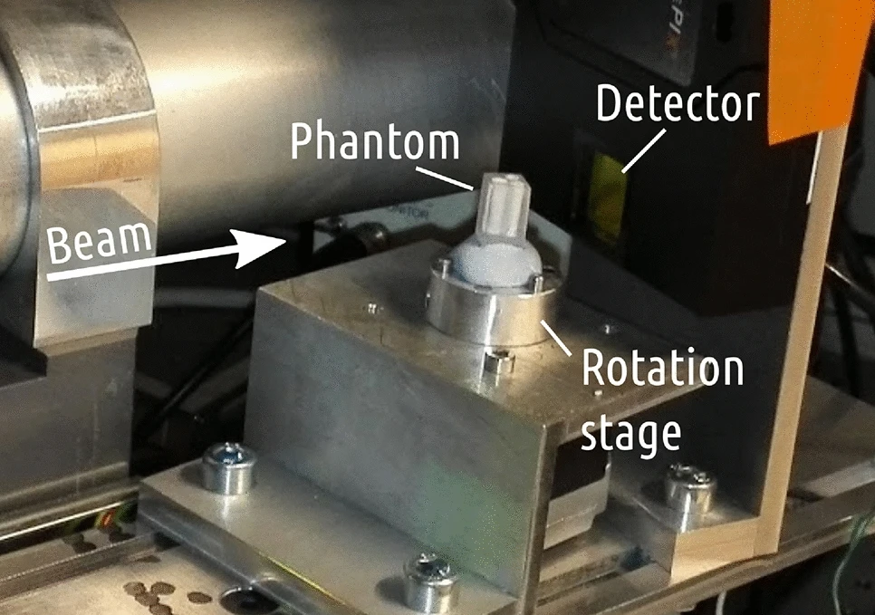
The phantom described in Section 4.1 was measured with a XAS-CT setup, see Figure 3. This kind of arrangement monochromatises the polychromatic X-rays from the X-ray tube when they travel through a spherically bent crystal analyser.


4.3 K-edges in X-ray attenuation
Our IP method works on its best when we investigate materials with X-ray energies which are near the K-edges of the materials. In X-ray absorption spectroscopy, the K-edge is a sudden increase in X-ray absorption, occurring when the energy of the X-rays is just above the binding energy of the atoms’ electron shell. The term is based on the International Union of Pure and Applied Chemistry (IUPAC) X-ray notation, where the atomic orbitals are labelled with letters K, L, M, N… and so on. The innermost electron shell is known as the K-shell.
Physically, the sudden increase in attenuation is caused by the photoelectric absorption of photons. For this interaction to occur, the photons must have more energy than the binding energy of the K-shell electrons (K-edge). A photon having an energy just above the binding energy of the electron is more likely to be absorbed than a photon having an energy just below the binding energy or significantly above it.
Figure 6 illustrates this. In the figure, we have the different attenuation values as a function of photon energies in keV:s. The plots show how the attenuation varies with three different materials, which are pure selenium Se (blue), Na2SeO3 (red) and PMMA (green). We can see the sudden increase in attenuation of the selenium containing samples at the measured X-ray energy range (black box). We can compare with the PMMAs attenuation values, which are very smooth at that energy range. Clear k-edges at the measured energy range make the differentiation of materials much easier for the used material decomposition. The attenuation values in figure 6 are based on the attenuation value tables on the NIST (National Institute of Standards and Technology) X-ray attenuation online simulator [11].

5 Results
In this section we show the results with the simulations and finally with real data. The section also includes a brief demonstration of the effect of the new regularization term. We have measured the quality of the simulations with some error measures, which will be explained below.
5.1 Error measures of the simulations
We were avoiding the inverse crime in our simulations by adding some noise and modelling error into our data. The noise level in the simulations was selected to be one percent, and we added modelling error by rotating the phantom 45 degrees and interpolating the difference.
We calculated quality measures for the simulations by comparing the original phantoms with the resulting reconstructions. The classical errors were calculated correspondingly than in [5]. We defined the -error
| (12) |
In addition to that we calculated the structural similarity index (SSIM) [13] and Haar wavelet-based perceptual similarity index (HaarPSI) [10]. We have written down the mean values of the errors for all the materials, by summing up the numerical errors of the different materials and dividing by three. The same holds for the mean pixel error, which we have then listed as a percentage of correctly classified pixels (Corr.pix %) in table 2.
5.2 Effect of the new regularization term
In this section we show how regularization effects to our reconstruction results with IP method, when using simulations. We use digital phantoms, because the point is just to demonstrate the effect of the inner product regularization parameter.
The coefficients which we used for the simulated materials with different energies are listed in the table 1.
| Energy | M1 | M2 | M3 |
|---|---|---|---|
| E1 | 22.73 | 8.56 | 3.51 |
| E2 | 5.95 | 12.32 | 10.88 |
| E3 | 7.81 | 3.51 | 27.77 |
We chose resolution for the reconstructions. The number of used projection images was sparse in these simulations: 15 equispaced angles.
After choosing the most optimal value, (here = 20000) we start to increase the parameter from zero, to see how it affects the result. See figure 8. The errors of the reconstructions, compared with the ground truth are listed in the table 2. We can see from the results that increasing the term reduces the error and improves the quality of the reconstructions. The range of is limited to be smaller than the parameter to ensure that the problem stays convex.
| Mean errors: | L2 | SSIM | haarPSI | Corr.pix % | ||
| First row: | 0.60 | 0.25 | 0.14 | 96 | 20000 | 0 |
| Second row: | 0.56 | 0.26 | 0.17 | 96.4 | 20000 | 8000 |
| Third row: | 0.55 | 0.39 | 0.19 | 96.3 | 20000 | 16000 |
| Fourth row: | 0.59 | 0.41 | 0.21 | 95.6 | 20000 | 19500 |
| Ground truth: | 0 | 1 | 1 | 100 |


5.3 Results with simulated data
We have simulated the real data case virtually by using the measured attenuation values of the selenium compounds 4. We have the error measures separately for each material in table 3.

| Material | Method | L2 | SSIM | HPSI |
|---|---|---|---|---|
| Se | IP | 0.27 | 0.87 | 0.42 |
| SeO3 | IP | 0.25 | 0.81 | 0.47 |
| SeO4 | IP | 0.20 | 0.89 | 0.54 |
5.4 Results with experimental X-ray data
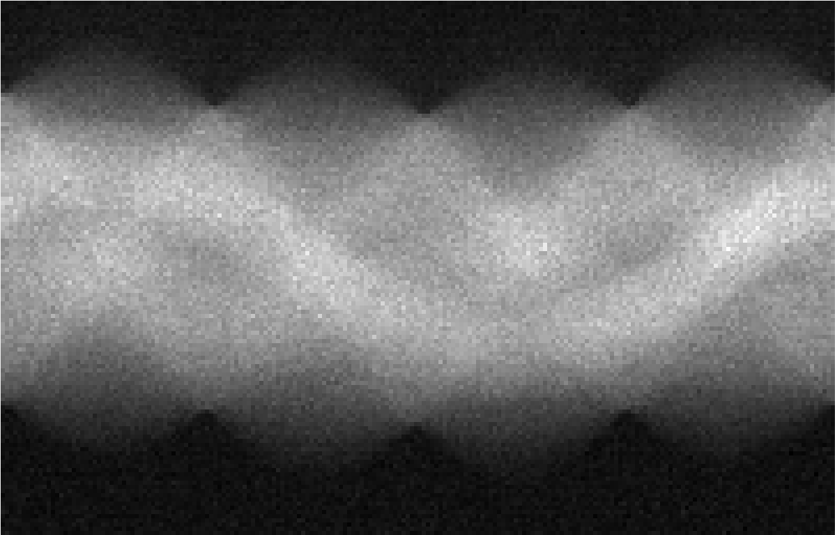
In this section, we show the reconstruction results with the standard filtered back projection (FBP) method and with the IP-method, see figure 10.
The number of used projection images is 200 with the real data. We used the X-ray attenuation coefficients determined in [8] in our system matrix, in place of the coefficients. The X-ray attenuation coefficients used with different X-ray energies are listed in Table 4.
| Energy [keV] | Se | SeO3 | SeO4 |
|---|---|---|---|
| 12.658 | 8.4734 | 2.4380 | 3.5091 |
| 12.662 | 7.9902 | 11.859 | 10.885 |
| 12.685 | 7.4175 | 8.0033 | 27.777 |
Our simulation studies reported in Section 5.3 suggest that and are suitable choices for the regularization parameters.
The reconstruction images in figure 10 have been black point and white point corrected for better visual impression. In these reconstructions, we have used all the projection images taken, so we have used data from 200 different projection angles. The first row of the figure shows FBP reconstructions made from the sinograms, which were measured with energies 12,658 keV, 12,662 keV and 12,685 keV. The end result is quite noisy and there are only small differences between the reconstructions. We have the PMMA phantom as a fourth material on the first row (and there was also some potassium as fulfilling material). The attenuation coefficients of these "extra" materials are quite same with every measured energy (they have no K-edges, see figure 6). This for, we subtracted one low energy sinogram 12,645 keV (which was below all the K-edges) from the other sinograms before reconstruction. The result can be seen on the second and third row in the figure, where we have got rid of the phantom matrix. We have the FBP reconstructions on the second row and the IP reconstructions of the different materials on the third row.
6 Conclusions
The Inner Product reconstruction approach seems to be capable for material decomposition in the case of real, monochromatic X-ray data. The reconstruction results show clearly where the different materials are located in the sample, even though there is some noticeable dotted noise around the samples. The theory of this method has been shown to work for multiple materials and X-ray energies and in this article we demonstrated the working in the case of three energies and three materials. As a drawback, we can notice that there must be clear difference in the attenuation coefficients of the materials with different energies for the proper working of the method. This is achieved using monochromatic X-ray beam and by selecting the used X-ray energies wisely just below and over the K-edge peak of the materials to be decomposed. When we keep these limitations in mind, the method works as a reliable and simple tool for material separation and identification.
References
- [1] Kees Joost Batenburg, Sara Bals, J Sijbers, C Kübel, PA Midgley, JC Hernandez, U Kaiser, ER Encina, EA Coronado, and G Van Tendeloo. 3d imaging of nanomaterials by discrete tomography. Ultramicroscopy, 109(6):730–740, 2009.
- [2] Kees Joost Batenburg and Jan Sijbers. Dart: a practical reconstruction algorithm for discrete tomography. IEEE Transactions on Image Processing, 20(9):2542–2553, 2011.
- [3] Joachim Baumann, Zoltán Kiss, Sven Krimmel, Attila Kuba, Antal Nagy, Lajos Rodek, Burkhard Schillinger, and Jürgen Stephan. Discrete tomography methods for nondestructive testing. In Advances in discrete tomography and its applications, pages 303–331. Springer, 2007.
- [4] J. Gondzio. Interior point methods 25 years later. European Journal of Operational Research, 218:587–601, 2012.
- [5] Jacek Gondzio, Matti Lassas, Salla-Maaria Latva-Äijö, Samuli Siltanen, and Filippo Zanetti. Material-separating regularizer for multi-energy x-ray tomography. Inverse Problems, 38(2):025013, 2022.
- [6] Gabor T Herman and Attila Kuba. Advances in discrete tomography and its applications. Springer Science & Business Media, 2008.
- [7] Gabor T Herman and Attila Kuba. Discrete tomography: Foundations, algorithms, and applications. Springer Science & Business Media, 2012.
- [8] Ari-Pekka Honkanen and Simo Huotari. Monochromatic computed tomography using laboratory-scale setup. Scientific Reports, 13(1):363, 2023.
- [9] Yong Long and Jeffrey A Fessler. Multi-material decomposition using statistical image reconstruction for spectral ct. IEEE transactions on medical imaging, 33(8):1614–1626, 2014.
- [10] Rafael Reisenhofer, Sebastian Bosse, Gitta Kutyniok, and Thomas Wiegand. A haar wavelet-based perceptual similarity index for image quality assessment. Signal Processing: Image Communication, 61:33–43, 2018.
- [11] EB Saloman, JH Hubbell, and JH Scofield. X-ray attenuation cross sections for energies 100 ev to 100 kev and elements z= 1 to z= 92. Atomic Data and Nuclear Data Tables, 38(1):1–196, 1988.
- [12] Rasmus Solem, Till Dreier, Isabel Gonçalves, and Martin Bech. Material decomposition in low-energy micro-ct using a dual-threshold photon counting x-ray detector. Frontiers in Physics, 9:673843, 2021.
- [13] Zhou Wang, Alan C Bovik, Hamid R Sheikh, and Eero P Simoncelli. Image quality assessment: from error visibility to structural similarity. IEEE transactions on image processing, 13(4):600–612, 2004.
- [14] S. J. Wright. Primal-Dual Interior-Point Methods. SIAM, 1997.
- [15] Weiwen Wu, Haijun Yu, Peijun Chen, Fulin Luo, Fenglin Liu, Qian Wang, Yining Zhu, Yanbo Zhang, Jian Feng, and Hengyong Yu. Dictionary learning based image-domain material decomposition for spectral ct. Physics in Medicine & Biology, 65(24):245006, 2020.
