A $R_{\rm V}$ map of the Milky Way revealed by LAMOST

The extinction law, also known as the extinction curve, represents the variation of extinction with wavelength or frequency. It plays a crucial role in correcting the effects of dust extinction in observed objects and has been extensively studied to understand the properties of dust grains. Fitzpatrick & Massa 1986; Fitzpatrick & Massa 1988 parameterized the extinction curve in the ultraviolet (UV) bands using a simple 6-parameter function. Cardelli et al. 1989 showed that the extinction curve from the UV to the optical (303 nm – 3.5 $\mu$m) can be described by a one-parameter family of curves with different values of the parameter $R_{\rm V}$. The $R_{\rm V}$ parameter, which is known as the total-to-selective extinction ratio, is defined as $R_{\rm V}\equiv A_{\rm V}/E(B-V)$. Much (but not all) of the spatial variability seen in extinction curves has been shown to correlate with $R_{\rm V}$. Consequently, this one-parameter description allows us to predict the extinction value at any wavelength within the optical to UV range, based solely on the knowledge of the $R_{\rm V}$ value along a particular line of sight. A smaller $R_{\rm V}$ value indicates a steeper extinction curve, implying a larger difference in extinction at different wavelengths. Since then, numerous studies have been conducted to model extinction curves, employing various fitting techniques and considering different sightlines and wavelength ranges (Fitzpatrick & Massa 1990; O’Donnell 1994; Maíz Apellániz et al. 2014; Fitzpatrick et al. 2019; Gordon et al. 2023a, e.g.,).

$R_{\rm V}$ not only serves as a parameter to describe extinction curves but also provides valuable information about the properties of dust grains. The model proposed by Weingartner & Draine 2001 demonstrated a correlation between larger average grain sizes and higher $R_{\rm V}$ values. However, other factors such as the chemical composition of dust grains may also contribute to the variation in $R_{\rm V}$ values. Observations of the diffuse interstellar medium in the Milky Way suggest an average $R_{\rm V}$ value of approximately 3.1 (Savage & Mathis 1979; Cardelli et al. 1989), but the variation in different sightlines can be very large. It is widely accepted that sightlines passing through dense molecular clouds with high extinction tend to exhibit higher $R_{\rm V}$ values, reaching values as large as approximately 6(Fitzpatrick 1999, e.g.,). This variation can be attributed to dust grain growth through processes such as accretion and coagulation (Vrba & Rydgren 1984; Fitzpatrick 1999; Draine 2003; Köhler et al. 2012; Foster et al. 2013, e.g.,). In low-density regions, $R_{\rm V}$ values could be as small as approximately 2 (Welty & Fowler 1992; Fitzpatrick 1999; Wang et al. 2017, e.g.,). When dust grains are fully exposed to radiation, they become more susceptible to destruction through processes such as sputtering by impinging atoms or ions, photolysis by UV photons, and photodesorption occurring on the dust surface (Draine 2003).

Prior to the 2010s, the number of O and B stars with accurate $R_{\rm V}$ measurements was limited to a few hundred (Fitzpatrick & Massa 2007, e.g.). However, the availability of precise stellar parameter measurements and intrinsic colors from modern large-scale astronomical surveys has opened up the possibility of measuring $R_{\rm V}$ values for large samples of stars across extensive sky regions. Schlafly et al. 2016 measured $R_{\rm V}$ values along 150,000 sightlines based on the APOGEE spectroscopic data and a series of photometric bands from the optical to the near-infrared (near-IR). They mapped the distribution of $R_{\rm V}$ in the nearby Galactic mid-plane (within a distance of $<$ 4 kpc) and found that most variations in $R_{\rm V}$ are not correlated with dust column density in the range of $0.5<E(B-V)<2$, but instead show a correlation with distance. Furthermore, S16 discovered a strong negative correlation between $R_{\rm V}$ and the dust emissivity spectral index $\beta$ between 353 and 3000 GHz, which suggests that conditions that lead to steep far-infrared emission spectra also lead to optical and infrared extinction curves become steeper. However, due to the sparse sampling of diverse environments, the detailed physical and chemical mechanisms underlying the variations in $R_{\rm V}$ are still unclear.

The Large Sky Area Multi-Object Fiber Spectroscopy Telescope (LAMOST; Zhao et al. 2012; Cui et al. 2012; Liu et al. 2014) has provided us with over 10 million high-quality stellar spectra and precise atmospheric parameters, enabling us to examine the spatial variability of $R_{\rm V}$ with greater spatial resolution and wider sky coverage. In our previous study (Zhang & Yuan 2023, hereafter ZY23), we accurately measured the reddening for 5 million stars across a wide range of wavelengths, achieving typical errors of 0.01-0.03 mag for individual colors.

Based on the results, we aim to construct a highly precise $R_{\rm V}$ map that spans from the Galactic disk to the halo by utilizing the extinction law of Fitzpatrick 1999 and the BOSZ synthetic spectral database (Bohlin et al. 2017). This map will enable us to investigate the physical properties of dust in unprecedented detail and provide valuable observational constraints on the formation and evolution of dust grains.

The paper is organized as follows. In Section II, we briefly introduce the adopted data sets. In Section III, we obtain $R_{\rm V}$ of each star by a forward modeling approach and check the reliability of the results. In Section IV, we present our $R_{\rm V}$ map and discuss its implications. In Section V, we compare the measurements with the study in the literature, investigate the spatial coincidence between $R_{\rm V}$ and molecular clouds, and study the correlation between $R_{\rm V}$ and some parameters of the interstellar medium (ISM). We summarize our findings in Section VI.

The data used in this study were obtained from our previous work, ZY23, which provided highly accurate reddening measurements for approximately 5 million stars across 21 different colors. The typical errors of the reddening values are only 0.01 – 0.03 mag, depending on color. For this study, we have selected specific colors from various passbands spanning the optical to mid-infrared wavelength range. These passbands include the $g/r/i/z/y$-band of Pan-STARRS 1 (PS1; Chambers & Pan-STARRS Team 2018), the $G_{\rm BP}/G/G_{\rm RP}$-band of $Gaia$, the $u/g/r/i/z$-band of Sloan Digital Sky Survey (SDSS; Alam et al. 2015), the $J/H/K_{\rm S}$-band of Two Micron All Sky Survey (2MASS; Skrutskie et al. 2006), and the $W1/W2$-band of Wide-field Infrared Survey Explorer (WISE; Wright et al. 2010). We excluded the passbands from the Galaxy Evolution Explorer (GALEX; Martin et al. 2005) and the $W3/W4$-band of WISE due to the limited number of sources with reliable photometric quality.

The stellar parameters used in the paper, including effective temperatures $T_{\rm eff}$, surface gravities ${\rm log}\,g$, and metallicities ${\rm[Fe/H]}$, have been derived from the LAMOST Stellar Parameter Pipeline (LASP) (Wu et al. 2011; Luo et al. 2015) and the HotPayne catalog of Xiang et al. 2022. The $E(B-V)$ values for each star are calculated using their corresponding $E(G_{\rm BP}-G_{\rm RP})$ and $R(G_{\rm BP}-G_{\rm RP})$ values, which were obtained from ZY23. Since the values of $R(G_{\rm BP}-G_{\rm RP})$ used in this study were obtained using the $E(B-V)$ values from the dust map of Schlegel et al. 1998 in the intermediate to high Galactic latitude regions, we have corrected for the 14% overestimation of SFD $E(B-V)$ values (Schlafly et al. 2010; Yuan et al. 2013).

Firstly, we utilize the same sample cleaning and trimming criteria as described in the data section of ZY23. Then, we binned the stars in our dataset by their values of $E(B-V)$ and $T_{\rm eff}$. Subsequently, we performed a 3$\sigma$ rejection of the reddening values for each color within each bin in the corresponding color excess - $E(B-V)$ diagram. These mitigate the impact of inaccurate reddening measurements in the subsequent analysis. On average, this step removes approximately 10–20% of color excesses.

To create the $R_{\rm V}$ map, we must initially determine the $R_{\rm V}$ value for each star in our sample. To achieve this, we used a forward modeling technique that compares simulated color excess ratios (CERs) with measured values to determine each star’s best-fit $R_{\rm V}$.

After verification, we find that differences in different dust models can lead to changes in the overall distribution of the sample’s measured $R_{\rm V}$, but have little impact on the relative difference of $R_{\rm V}$. We compared the measured data with F99 and the models of Fitzpatrick et al. 2019 and Gordon et al. 2023b. Our preliminary analysis shows that the F99 model fits better for the color excess of this sample, and therefore the F99 model is used for calculations in the follow-up process. It is worth noting that the evaluation of other extinction laws requires a dedicated study, but this is beyond the scope of this paper.

We adopted the F99 reddening law to characterize the $R_{\rm V}$-dependent extinction curves, expressed as $A_{\lambda}/A_{\rm V}$, where $A_{\lambda}$ represents the extinction at a specific wavelength $\lambda$, and $A_{\rm V}$ is the V-band extinction. The F99 reddening law has been widely used in literature and is consistent with observational data, as demonstrated in previous studies such as Schlafly & Finkbeiner 2011 and Yuan et al. 2013. For a given star, the extinction at a specific passband $x$ can be expressed as,

where $\lambda$ is the wavelength, $h$ is the Planck constant, $c$ is the speed of light, $F_{0}(\lambda)$ is the intrinsic flux of the star, $S(\lambda)$ the filter response curve of the passband $x$, and $R(\lambda)$ the extinction term. According to the F99 extinction law, $R(\lambda)$ can be expressed as,

In this study, we utilized the intrinsic flux $F_{0}(\lambda)$ from the BOSZ stellar atmosphere models database (Bohlin et al. 2017) and the filter profiles $S(\lambda)$ of the individual passbands from Rodrigo & Solano 2020. We only used the BOSZ spectra with stellar parameters of ${\rm[Fe/H]}$ = 0, [$\alpha$/H] = 0, and [C/H] = 0, as varying ${\rm[Fe/H]}$, [$\alpha$/H], or [C/H] has negligible impact on the results. Additionally, to obtain templates of $A_{x}$, we adopted a grid that covers the following parameter ranges: $T_{\rm eff}$ from 3750 to 20000 K in steps of 250 K for $T_{\rm eff}\leq$ 7500 K and 500 K for $T_{\rm eff}\geq$ 7500 K, $E(B-V)$ from 0 to 3 mag, with a step size of 0.01 mag for $E(B-V)<0.2$ mag, 0.04 mag for $0.2<E(B-V)<1$ mag, and 0.25 mag for $E(B-V)>1$ mag, ${\rm log}\,g$ from 0 to 5 with a step size of 0.5, and $R_{\rm V}$ from 1 to 7 with a step size of 0.1.

To derive the best-fit $R_{\rm V}$ values, we simulated the CERs using the expression $E(x-RP)/E(BP-RP)=({A_{x}-A_{RP})/(A_{BP}-A_{RP}})$, and then compared them with observations. This form of CER was used because we lack absolute extinction measurements for individual stars and only have reddening data. Among the photometric bands in our dataset, $Gaia$ photometry provides the largest sample size and the highest degree of accuracy. In addition, our previous research has shown that the model reddening coefficients for the $Gaia$ filters align well with empirical coefficients, thereby reducing potential uncertainties. In Fig. 1 we show the simulated CERs as functions of the $R_{\rm V}$, $E(B-V)$, and $T_{\rm eff}$ parameters. We note that CERs for $z$ and $W1$ filters at $T_{\rm eff}$ = 4000 K (the reddest lines in the bottom middle and right panels, respectively) appear abnormal, probably due to the potential issues with the BOSZ model in those IR bands and at low temperature.

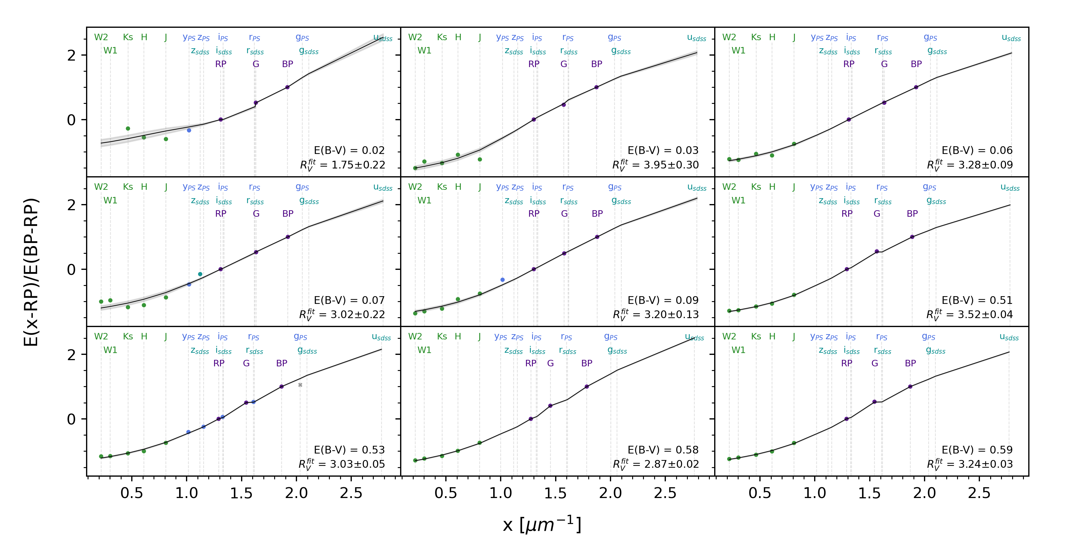
We used the linear least squares estimation method curve_fit of the SciPy module (Virtanen et al. 2020) to obtain the best-fit $R_{\rm V}$ values for individual stars in our sample. We first identified the nearest grid point to the measured $T_{\rm eff}$ and $E(B-V)$. Subsequently, we performed a linear interpolation of the $R_{\rm V}$ grid points to find the optimal $R_{\rm V}$ value that minimized the differences between the measured and simulated CERs. During this process, we also estimated the standard deviation error, denoted as $err(R_{\rm V})$. In our analysis, only stars with a minimum of five CERs (including both the $Gaia$ $BP$ and $RP$ bands) were considered. Fig. 2 illustrates several examples of the $R_{\rm V}$ fits. Overall, the model CERs exhibit a good agreement with the measured values. Furthermore, the dispersion and estimated errors decrease with increasing extinction.

We have constructed mock data to test our method. The simulation revealed there is a systematic underestimation of the $R_{\rm V}$ values obtained at low extinction. For example, for mock samples with $R_{\rm V}$ of 3.1 and corresponding $E(B-V)$ values of 0.05 and 0.02, the measured $R_{\rm V}$ would be underestimated by 0.2 and 1.4, respectively. Subsequent analysis indicated that such systematic errors become negligible when $E(B-V)\geq 0.1$, and we defined this threshold as the criterion for the ‘reliable’ sample. Consequently, it is essential to develop a more refined approach to obtain well-measured $R_{\rm V}$ values at low extinction regions in the future.

Finally, we have obtained a total of 3,182,038 valid $R_{\rm V}$ measurements, out of which 1,178,719 are considered reliable. The values and errors of the reliable sample are displayed in Fig. 3. The density contours reveal a concentration of results around $R_{\rm V}=3.2$ and $err(R_{\rm V})=0.05$. Notably, there is a positive correlation between $R_{\rm V}$ and $err(R_{\rm V})$, which is more pronounced for stars with high $E(B-V)$. This correlation arises primarily from the increased sensitivity of the F99 extinction curve to changes in $R_{\rm V}$ as $R_{\rm V}$ values increase, consequently causing larger $err(R_{\rm V})$.

To investigate potential correlations between best-fit $R_{\rm V}$ values and stellar parameters, we have selected stars located in a specific region at the edge of the Taurus complex ($l$ = 172.5 – 174.5° and $b$ = $-22$ – $-20.5$°). After excluding stars with $err(R_{\rm V})>0.1$, we have plotted the distribution of $R_{\rm V}$ and $err(R_{\rm V})$ in the $T_{\rm eff}$-${\rm log}\,g$ diagram, as shown in Fig. 4. Furthermore, we have examined the correlations between $R_{\rm V}$ and several stellar parameters, including $T_{\rm eff}$, ${\rm log}\,g$, [Fe/H], $M_{G}$, $E(B-V)$, $d$, and $err(R_{\rm V})$, which are displayed in Fig. 5. $M_{G}$ values are calculated using the $G$-band extinction coefficient, observed $G$ magnitude, and distance from $Gaia$ DR3 (Gaia Collaboration et al. 2021). Overall, our findings indicate that $R_{\rm V}$ values are generally independent of these parameters, as expected. However, the $R_{\rm V}$ values are slightly larger for giant stars at $T_{\rm eff}$ = 4000 K. This may be partly attributed to the large uncertainties resulting from the inability of the BOSZ stellar models to accurately predict the near-IR flux of low-temperature stars.

To create a 2D map of $R_{\rm V}$, we divided the validly measured stars into small pixels. In this study, we partition the celestial sphere into 196,608 sightlines by using the HEALPix scheme ($nside=128$, a spatial resolution of $\sim$ 27.5 arcmin). After applying a 3-$\sigma$ clipping for each sightline, we calculate the median $R_{\rm V}$ and $E(B-V)$ values. We do not use the weighted average algorithm due to the positive correlation between $R_{\rm V}$ and $err(R_{\rm V})$, which can cause systematic underestimations of $R_{\rm V}$. We also excluded sightlines with less than five sources, which are primarily distributed at high Galactic latitudes. The resulting 2D $R_{\rm V}$ map is shown in Fig. 6.

Fig. 6 presents the distribution of $R_{\rm V}$ across a wide expanse of our Galaxy, encompassing regions ranging from the Galactic disk to the halo. The $R_{\rm V}$ measurements in the Milky Way exhibit significant variations across different regions, with values spanning from 2.0 to 4.5. Notably, these values do not follow a random pattern but exhibit small-scale and large-scale variations throughout the Milky Way. Specifically, $R_{\rm V}$ values are higher in certain regions, such as those with Galactic coordinates of $l=180-210$° and $b<10$°, $l=60-120$° and $|b|<15$°, and near $-30<l<30$° and $b=30$°. Conversely, $R_{\rm V}$ values are lower in regions such as those with coordinates near $l=140-16$0° and $|b|<20$°, and of $l=25-60$° and $b=-20-10$°. Apart from these large-scale patterns, the $R_{\rm V}$ values also exhibit fine-scale structures down to the scales inside individual molecular clouds.

As shown in Fig. 6, the distribution of $R_{\rm V}$ in the low extinction region with a median $E(B-V)$ less than 0.1 (indicated by black contours) appears to exhibit a high degree of randomness. This is primarily due to the significant errors in the measured CERs resulting from low reddening values. To obtain a robust $R_{\rm V}$ distribution, it is necessary to eliminate sightlines with large errors. Additionally, the gray lines on the map highlight the transition region with $0.05<E(B-V)<0.1$, indicating that measurements of $R_{\rm V}$ within these regions should be used with caution. In subsequent analyses, we constructed a 2D map using reliable samples instead of considering all valid measurements. Furthermore, we employ the median absolute deviation (MAD) and standard deviation (STD) values to identify a set of ‘reliable’ sightlines. A sightline is deemed reliable if $mad/R_{\rm V}<10\%$, $std/R_{\rm V}<15\%$, and the number of reliable stars $N>5$. As a result, 71% sightlines were eliminated and remained 24,795 reliable sightlines.

The histograms of the best-fit $R_{\rm V}$ values for individual stars and the median $R_{\rm V}$ values for the individual sightlines are shown in Fig. 7. The distribution of $R_{\rm V}$ for all stars in the catalog is non-Gaussian, which may be partly due to the large measurement error for stars with low extinction, and partly because the intrinsic distribution may well be non-Gaussian. However, the distribution of $R_{\rm V}$ values for the reliable sample closely follows a Gaussian shape, with a slight excess in the higher $R_{\rm V}$ end. The mean $R_{\rm V}$ for the reliable sample is 3.24, with a dispersion of 0.34. This result slightly differs from the findings of Schlafly et al. 2016 (who reported $\mu=3.32$ and $\sigma=0.18$) due to variations in the $R_{\rm V}$ calculation methods and the traced regions, as discussed in Section V. The median $R_{\rm V}$ values for individual sightlines show a narrower distribution in the bottom panel of Fig. 7. For the selected reliable sightlines, the distribution is well described by a Gaussian with a mean of 3.25 and a standard deviation of 0.25.

Using high-precision CERs between colors from the optical to the mid-IR, we have measured the $R_{\rm V}$ values of about 3 million LAMOST stars in our study. To account for the combined impact of stellar SED and extinction, we have developed a robust forward modeling approach based on a model constructed using BOSZ stellar spectra and the F99 extinction curve. To validate our results, we compared our derived $R_{\rm V}$ values with the literature and found good agreement. We have divided the sample stars into different sightlines and calculated the median $R_{\rm V}$ value for each direction. This allowed us to create a 2D $R_{\rm V}$ map within the LAMOST footprint, spanning from the Galactic disk to the Galactic halo. Based on the analysis of reliable sightlines, we summarize our findings as follows:

1. 1.

   Overall, the distribution of $R_{\rm V}$ is well-described by a Gaussian distribution with a mean of 3.25 and a dispersion of 0.25, with a slight excess at the high end. The variability of $R_{\rm V}$ within the Galactic disk exhibits a wide range, manifesting at various scales from small structures within individual molecular clouds to larger scales spanning kiloparsecs.

2. 2.

   The spatial distribution of $R_{\rm V}$ closely aligns with the shape of molecular clouds. Specifically, we observe lower $R_{\rm V}$ values within the interior regions of molecular clouds compared to their surrounding areas. Although the average $R_{\rm V}$ may vary across different molecular clouds, this coincidence suggests that molecular clouds play a crucial role in the chemical and size evolution of dust grains.

3. 3.

   In the $E(B-V)$ interval ranging from 0.1 to 1.25, we find that $R_{\rm V}$ is largely independent of extinction. Additionally, we have investigated the correlations between $R_{\rm V}$ and other interstellar parameters, such as $T_{\rm dust}$, $\beta$, $N_{\rm HI}$, $N_{\rm H_{2}}$, $N_{\rm H_{2}}/N_{\rm HI}$, and $GDR$. Notably, we observe that these relationships vary with the level of extinction, providing valuable insights into the diverse properties of dust in different interstellar environments.

In addition to giving us further insight into the physics of the dust, the $R_{\rm V}$ map also helps us to do precision extinction correction. After correcting the all-sky two-dimensional (2D) reddening map (Sun et al. 2022) and investigating the temperature and extinction dependence of reddening coefficients (Zhang & Yuan 2023), in this study, we also laid foundation for addressing the third challenge outlined in ZY23, i.e., the significant impact of the spatial variation of $R_{\rm V}$ on extinction corrections. In the future, we will synthesize factors to create an accurate extinction correction toolkit.

References

- Alam et al. (2015) Alam, S., Albareti, F. D., Allende Prieto, C., et al. 2015, ApJS, 219, 12, doi: 10.1088/0067-0049/219/1/12
- Bohlin et al. (2017) Bohlin, R. C., Mészáros, S., Fleming, S. W., et al. 2017, AJ, 153, 234, doi: 10.3847/1538-3881/aa6ba9
- Bolatto et al. (2013) Bolatto, A. D., Wolfire, M., & Leroy, A. K. 2013, ARA&A, 51, 207, doi: 10.1146/annurev-astro-082812-140944
- Cardelli et al. (1989) Cardelli, J. A., Clayton, G. C., & Mathis, J. S. 1989, ApJ, 345, 245, doi: 10.1086/167900
- Chambers & Pan-STARRS Team (2018) Chambers, K., & Pan-STARRS Team. 2018, in American Astronomical Society Meeting Abstracts, Vol. 231, American Astronomical Society Meeting Abstracts #231, 102.01
- Cui et al. (2012) Cui, X.-Q., Zhao, Y.-H., Chu, Y.-Q., et al. 2012, Research in Astronomy and Astrophysics, 12, 1197, doi: 10.1088/1674-4527/12/9/003
- Draine (2003) Draine, B. T. 2003, ARA&A, 41, 241, doi: 10.1146/annurev.astro.41.011802.094840
- Fitzpatrick (1999) Fitzpatrick, E. L. 1999, PASP, 111, 63, doi: 10.1086/316293
- Fitzpatrick & Massa (1986) Fitzpatrick, E. L., & Massa, D. 1986, ApJ, 307, 286, doi: 10.1086/164415
- Fitzpatrick & Massa (1988) —. 1988, ApJ, 328, 734, doi: 10.1086/166332
- Fitzpatrick & Massa (1990) —. 1990, ApJS, 72, 163, doi: 10.1086/191413
- Fitzpatrick & Massa (2007) —. 2007, ApJ, 663, 320, doi: 10.1086/518158
- Fitzpatrick et al. (2019) Fitzpatrick, E. L., Massa, D., Gordon, K. D., Bohlin, R., & Clayton, G. C. 2019, ApJ, 886, 108, doi: 10.3847/1538-4357/ab4c3a
- Foster et al. (2013) Foster, J. B., Mandel, K. S., Pineda, J. E., et al. 2013, MNRAS, 428, 1606, doi: 10.1093/mnras/sts144
- Gaia Collaboration et al. (2021) Gaia Collaboration, Brown, A. G. A., Vallenari, A., et al. 2021, A&A, 649, A1, doi: 10.1051/0004-6361/202039657
- Gordon et al. (2023a) Gordon, K. D., Clayton, G. C., Decleir, M., et al. 2023a, arXiv e-prints, arXiv:2304.01991, doi: 10.48550/arXiv.2304.01991
- Gordon et al. (2023b) —. 2023b, ApJ, 950, 86, doi: 10.3847/1538-4357/accb59
- Irfan et al. (2019) Irfan, M. O., Bobin, J., Miville-Deschênes, M.-A., & Grenier, I. 2019, A&A, 623, A21, doi: 10.1051/0004-6361/201834394
- Köhler et al. (2012) Köhler, M., Stepnik, B., Jones, A. P., et al. 2012, A&A, 548, A61, doi: 10.1051/0004-6361/201218975
- Liu et al. (2014) Liu, X. W., Yuan, H. B., Huo, Z. Y., et al. 2014, in Setting the scene for Gaia and LAMOST, ed. S. Feltzing, G. Zhao, N. A. Walton, & P. Whitelock, Vol. 298, 310–321, doi: 10.1017/S1743921313006510
- Luo et al. (2015) Luo, A. L., Zhao, Y.-H., Zhao, G., et al. 2015, Research in Astronomy and Astrophysics, 15, 1095, doi: 10.1088/1674-4527/15/8/002
- Maíz Apellániz et al. (2014) Maíz Apellániz, J., Evans, C. J., Barbá, R. H., et al. 2014, A&A, 564, A63, doi: 10.1051/0004-6361/201423439
- Martin et al. (2005) Martin, D. C., Fanson, J., Schiminovich, D., et al. 2005, ApJ, 619, L1, doi: 10.1086/426387
- O’Donnell (1994) O’Donnell, J. E. 1994, ApJ, 422, 158, doi: 10.1086/173713
- Planck Collaboration et al. (2016) Planck Collaboration, Adam, R., Ade, P. A. R., et al. 2016, A&A, 594, A10, doi: 10.1051/0004-6361/201525967
- Rodrigo & Solano (2020) Rodrigo, C., & Solano, E. 2020, in XIV.0 Scientific Meeting (virtual) of the Spanish Astronomical Society, 182
- Savage & Mathis (1979) Savage, B. D., & Mathis, J. S. 1979, ARA&A, 17, 73, doi: 10.1146/annurev.aa.17.090179.000445
- Schlafly & Finkbeiner (2011) Schlafly, E. F., & Finkbeiner, D. P. 2011, ApJ, 737, 103, doi: 10.1088/0004-637X/737/2/103
- Schlafly et al. (2010) Schlafly, E. F., Finkbeiner, D. P., Schlegel, D. J., et al. 2010, ApJ, 725, 1175, doi: 10.1088/0004-637X/725/1/1175
- Schlafly et al. (2016) Schlafly, E. F., Meisner, A. M., Stutz, A. M., et al. 2016, ApJ, 821, 78, doi: 10.3847/0004-637X/821/2/78
- Schlegel et al. (1998) Schlegel, D. J., Finkbeiner, D. P., & Davis, M. 1998, ApJ, 500, 525, doi: 10.1086/305772
- Skrutskie et al. (2006) Skrutskie, M. F., Cutri, R. M., Stiening, R., et al. 2006, AJ, 131, 1163, doi: 10.1086/498708
- Snow & McCall (2006) Snow, T. P., & McCall, B. J. 2006, ARA&A, 44, 367, doi: 10.1146/annurev.astro.43.072103.150624
- Sun et al. (2022) Sun, Y., Yuan, H., & Chen, B. 2022, ApJS, 260, 17, doi: 10.3847/1538-4365/ac642f
- Virtanen et al. (2020) Virtanen, P., Gommers, R., Oliphant, T. E., et al. 2020, Nature Methods, 17, 261, doi: 10.1038/s41592-019-0686-2
- Vrba & Rydgren (1984) Vrba, F. J., & Rydgren, A. E. 1984, ApJ, 283, 123, doi: 10.1086/162281
- Wang et al. (2017) Wang, S., Jiang, B. W., Zhao, H., Chen, X., & de Grijs, R. 2017, ApJ, 848, 106, doi: 10.3847/1538-4357/aa8db7
- Weingartner & Draine (2001) Weingartner, J. C., & Draine, B. T. 2001, ApJ, 548, 296, doi: 10.1086/318651
- Welty & Fowler (1992) Welty, D. E., & Fowler, J. R. 1992, ApJ, 393, 193, doi: 10.1086/171497
- Wright et al. (2010) Wright, E. L., Eisenhardt, P. R. M., Mainzer, A. K., et al. 2010, AJ, 140, 1868, doi: 10.1088/0004-6256/140/6/1868
- Wu et al. (2011) Wu, Y., Luo, A. L., Li, H.-N., et al. 2011, Research in Astronomy and Astrophysics, 11, 924, doi: 10.1088/1674-4527/11/8/006
- Xiang et al. (2022) Xiang, M., Rix, H.-W., Ting, Y.-S., et al. 2022, A&A, 662, A66, doi: 10.1051/0004-6361/202141570
- Yuan et al. (2013) Yuan, H. B., Liu, X. W., & Xiang, M. S. 2013, MNRAS, 430, 2188, doi: 10.1093/mnras/stt039
- Zhang & Yuan (2023) Zhang, R., & Yuan, H. 2023, ApJS, 264, 14, doi: 10.3847/1538-4365/ac9dfa
- Zhao et al. (2012) Zhao, G., Zhao, Y.-H., Chu, Y.-Q., Jing, Y.-P., & Deng, L.-C. 2012, Research in Astronomy and Astrophysics, 12, 723, doi: 10.1088/1674-4527/12/7/002